Integrating Randomized Placebo-Controlled Trial Data with External Controls: A Semiparametric Approach with Selective Borrowing

Abstract

In recent years, real-world external controls (ECs) have grown in popularity as a tool to empower randomized placebo-controlled trials (RPCTs), particularly in rare diseases or cases where balanced randomization is unethical or impractical. However, as ECs are not always comparable to the RPCTs, direct borrowing ECs without scrutiny may heavily bias the treatment effect estimator. Our paper proposes a data-adaptive integrative framework capable of preventing unknown biases of ECs. The adaptive nature is achieved by dynamically sorting out a set of comparable ECs via bias penalization. Our proposed method can simultaneously achieve (a) the semiparametric efficiency bound when the ECs are comparable and (b) selective borrowing that mitigates the impact of the existence of incomparable ECs. Furthermore, we establish statistical guarantees, including consistency, asymptotic distribution, and inference, providing type-I error control and good power. Extensive simulations and two real-data applications show that the proposed method leads to improved performance over the RPCT-only estimator across various bias-generating scenarios.

Keywords: Adaptive LASSO; Calibration weighting; Dynamic borrowing; Selection Bias; Study Heterogeneity.

1 Introduction

Randomized controlled trials (RCTs) have been considered the gold standard of clinical research to provide confirmatory evidence on the safety and efficacy of treatments. However, RCTs are expensive, require lengthy recruitment periods, and may not always be ethical, feasible, or practical in rare or life-threatening diseases. In response to the 21st Century Cures Act, quality patient-level real-world data (RWD) from disease registries and electronic health records have become increasingly available and can generate fit-for-purpose real-world evidence to facilitate healthcare and regulatory decision-making (Food and Drug Administration, 2021). RWD have several advantages over RCTs. They include longer observation windows, larger and more heterogeneous patient populations, and reduce burden to investigators and patients (Visvanathan et al., 2017; Colnet et al., 2020). Drug developers and regulatory agencies are particularly interested in novel clinical trial designs that leverage external control subjects from RWD to improve the efficiency of randomized placebo-controlled trials (RPCTs) while maintaining robust evidence on the safety and efficacy of treatments (Silverman, 2018; Food and Drug Administration, 2019; Ghadessi et al., 2020). The focus of this paper is on hybrid control arm designs using RWD, where a RPCT enrolls a control arm that is augmented with real-world external controls (ECs) to form a hybrid comparator group.

1.1 Hybrid controls in the prior literature

The concept of hybrid controls dates back to Pocock (1976), who combined RPCTs and historical control data by adjusting for data-source level differences. Since then, numerous methods for using ECs have been developed. However, regulatory approvals using external control arm designs as confirmatory trials are rare and limited to ultra-rare diseases, pediatric trials, or oncology trials (Food and Drug Administration, 2014, 2016; Odogwu et al., 2018). Concerns regarding the validity and comparability of ECs from RWD have limited their use in a broader context. Guidance documents from regulatory agencies, including the recent Food and Drug Administration (FDA) draft guidance on Considerations for the Design and Conduct of Externally Controlled Trials for Drug and Biological Products, note several potential issues with ECs including selection bias, lack of concurrency, differences in the definitions of covariates, treatments, or outcomes, and unmeasured confounding (Food and Drug Administration, 2001, 2019, 2023). Each of these concerns can result in biased treatment effect estimates if ECs from RWD are integrated with RPCTs, which can lead to misleading conclusions. Significant efforts have been made to develop methodology to select ECs and adjust for potential differences between RPCTs and RWD to mitigate these biases.

Selection bias is a type of effect heterogeneity often encountered in non-randomized studies. In the context of EC augmentation, it arises when the RWD baseline subjects’ characteristics differ from those of the RPCT subjects. Multiple methods are available to adjust for selection bias by balancing the baseline covariates’ distributions across the different data sources. For example, matching and subclassification approaches select a subset of comparable ECs to construct the hybrid control arm (Stuart, 2010). Matching on the propensity score or the probability of trial inclusion can balance numerous baseline covariates simultaneously (Rosenbaum and Rubin, 1983a). Weighting approaches that re-weight ECs using the probability of trial inclusion or other balancing scores have also been proposed, e.g., empirical likelihood (Qin et al., 2015), entropy balancing (Lee et al., 2022; Chu et al., 2022; Wu and Yang, 2022b), constrained maximum likelihood (Chatterjee et al., 2016; Zhang et al., 2020), and Bayesian power priors (Neuenschwander et al., 2010; van Rosmalen et al., 2018).

Differences in the outcome distributions may still exist between RPCT and RWD control subjects after matching or weighting due to differences in study settings, time frame, data quality, or definition of covariates or outcomes (Phelan et al., 2017). Methods were proposed to adaptively select the degree of borrowing or adjust the outcomes for ECs based on observed differences in outcomes with the concurrent RPCT controls. Viele et al. (2014) used a hypothesis test on the expected control outcome to inform whether to incorporate all RWD subjects or no subjects into the hybrid control arm. More flexible borrowing approaches were also proposed including matching and bias adjustment (Stuart and Rubin, 2008), power priors (Ibrahim and Chen, 2000; Neuenschwander et al., 2009), Bayesian hierarchical models including meta-analytic predictive priors (Neuenschwander et al., 2010; Schoenfeld et al., 2019), and commensurate priors (Hobbs et al., 2011). While these existing methods seem appealing, simulation studies could not identify a single approach that could perform well across all scenarios where hidden biases exist (Shan et al., 2022). The surveyed Bayesian methods often resulted in inflated type I error while Frequentist methods resulted in large standard errors and lower power when hidden biases existed. Nearly all methods performed poorly in the presence of unmeasured confounding and could not simultaneously minimize bias and gain power. Further, many existing methods rely on parametric assumptions that are sensitive to model misspecification and cannot capture complex relationships that are prevalent in practice.

1.2 Contributions

We propose an approach to achieve efficient estimation of treatment effects that is robust to various potential discrepancies that may arise with ECs from RWD.

When handling the selection bias of ECs, our proposal is based on the calibration weighting (CW) strategy (Lee et al., 2022) to learn the weights of ECs so that the covariate distribution of ECs matches with that of the RPCT subjects. Furthermore, leveraging semiparametric theory, we develop an augmented CW (ACW) estimator, motivated by the efficient influence function (EIF; Bickel et al., 1998; Tsiatis, 2006), which is semiparametrically efficient and doubly robust against model misspecification. Moreover, it can incorporate flexible machine learning methods while maintaining the desirable parametric rate of convergence. Despite the potential to view the selection bias problem as a generalizability or transportability issue (Lee et al., 2022), our EIF fundamentally diverges from theirs as our context encompasses outcomes from both RPCTs and ECs, while Lee et al. solely considered RPCT outcomes.

To deal with potential outcome heterogeneity, we develop a selective borrowing framework to select only EC subjects that are comparable with RPCT controls for integration. Specifically, we introduce a bias parameter for each EC subject entailing his or her comparability with the similar RPCT control. To prevent bias in the integrative estimator from incomparable ECs, the goal is to select the comparable ECs with zero bias and exclude any ECs with non-zero bias. Thus, this formulation reframes the selective borrowing strategy as a model selection problem, which can be solved by penalized estimation (e.g., the adaptive LASSO penalty; Zou, 2006). Subsequent to the selection process, the comparable external controls are utilized to construct the ACW estimator. Prior works such as those by Chen et al. (2021), Liu et al. (2021) and Zhai and Han (2022) although able to identify biases, exclude the entire EC sample when confronted with incomparable ECs. Our approach introduces bias parameters at the subject level, which allows us to select comparable ECs only for integration. Moreover, compared to these existing selective borrowing approaches, our method leverages off-the-shelf machine learning models to achieve semiparametric efficiency and does not require strigent parametric assumptions on the distribution of outcomes.

The rest of the paper is organized as follows. Section 2 presents the asymptotic properties of the proposed semiparametric approach with selective borrowing. Sections 3 and 4 evaluate the performance of the proposed estimator in simulations and a real-data analysis. Section 5 provides an extension to deal with multiple EC groups. Section 6 concludes with a discussion.

2 Methodology

2.1 Notation, assumptions, and objectives

Let $\mathcal{R}$ represent a randomized placebo-controlled trial and $\mathcal{E}$ represent an external control source, which contain $N_{\mathcal{R}}$ and $N_{\mathcal{E}}$ subjects, respectively. The total sample size is $N=N_{\mathcal{R}}+N_{\mathcal{E}}$. An extension to multiple EC groups is discussed in Section 5. A total of $N_{t}$ and $N_{c}$ subjects receive the active treatment and control treatment in $\mathcal{R}$, while we assume all $N_{\mathcal{E}}$ subjects in $\mathcal{E}$ receive the control treatment. Each observation $i\in\mathcal{R}$ comprise the outcomes $Y_{i}$, the treatment assignment $A_{i}$, and a set of baseline covariates $X_{i}$. Similarly, each observation $i\in\mathcal{E}$ comprise $Y_{i}$, $A_{i}$, and $X_{i}$. Let $R_{i}$ represent a data source indicator, which is $1$ for all subjects $i\in\mathcal{R}$ and is $0$ for all subjects $i\in\mathcal{E}$. To sum up, an independent and identically distributed sample $\{V_{i}:i\in\mathcal{R}\cup\mathcal{E}\}$ is observed, where $V=(X,A,Y,R)$. Let $Y(a)$ denote the potential outcomes under treatment $a$ Rubin (1974). The causal estimand of interest is defined as the average treatment effect among the trial population, $\tau=\mu_{1}-\mu_{0}$, where $\mu_{a}={E}\{Y(a)\mid R=1\}$ for $a=0,1$. To link the observed outcome with the potential outcomes, we make the classical causal consistency assumption of $Y=AY(1)+(1-A)Y(0)$.

The gold-standard RPCT for treatment effect estimation satisfies the following assumption.

Assumption 1 (Randomization and positivity).

(i) $Y(a)\perp\!\!\!\perp A\mid(X,R=1)$ for $a=0,1,$ and (ii) the known treatment propensity score satisfies that $\pi_{A}(x)=P(A=1\mid X=x,R=1)>0$ for all $x$ s.t. $P(X=x,R=1)>0$.

Assumption 1 is standard in the causal inference literature (Rosenbaum and Rubin, 1983b; Imbens, 2004) and holds for the well-controlled clinical trials guaranteed by the randomization mechanism. Under Assumption 1, $\tau$ is identifiable from the RPCT data.

Moreover, the ECs should ideally be comparable with the concurrent RPCT subjects.

Assumption 2 (External control compatibility).

(i) ${E}\left\{Y(0)\mid X=x,R=0\right\}={E}\{Y(0)\mid X=x,R=1\}$, and (ii) $P(R=1\mid X=x)>0$ for all $x$ s.t. $P(X=x,R=0)>0$.

Assumption 2 states that the outcome mean function is equal for the RPCT and ECs. This assumption holds if $X$ captures all the outcome predictors that are correlated with $R$. In the FDA draft guidance (Food and Drug Administration, 2023) for drug development in rare diseases, there are five main concerns regarding the use of ECs: (i) selection bias, (ii) unmeasured confounding, (iii) lack of concurrency, (iv) data quality, and (v) outcome validity. Assumption 2 does not require the covariate distribution of the ECs to be the same as that of the RPCT. This is termed as the selection bias in the FDA draft guidance. Under Assumption 2, borrowing ECs to improve ATE estimation is similar to a transportability or covariate shift problem. However, the presence of concerns (ii)–(v) can result in violation of Assumption 2. Our paper has two main objectives: 1) Under Assumption 2, we develop a semiparametrically efficient and robust strategy to borrow ECs to improve ATE estimation while correcting for selection bias (Section 2.2); 2) Considering that Assumption 2 can be potentially violated, we incorporate a selective borrowing procedure that will detect the biases and retain only a subset of comparable ECs for estimation (Section 2.3).

2.2 Semiparametric efficient estimation under the ideal situation

2.2.1 Efficient influence function

Under the semiparametric theory (Bickel et al., 1998), we derive efficient and robust estimators for $\tau$ under Assumptions 1 and 2. The semiparametric model is attractive, because it exploits the information in the available data without making assumptions about the nuisance parts of the data generating process that are not of substantive interest. We derive the efficient influence function (EIF) of $\tau$. The theorem below shall serve as the foundational component of our proposed framework.

Theorem 1.

Under Assumptions 1 and 2, the EIF of $\tau$ is

$$\psi_{\tau,\mathrm{eff}}(V;\mu_{1},\mu_{0},q,r)=\frac{R}{P(R=1)}\left[\{\mu_{1}(X)-\mu_{0}(X)-\tau\}+\frac{A\{Y-\mu_{1}(X)\}}{\pi_{A}(X)}\right]\\ -\frac{R(1-A)+(1-R)r(X)}{P(R=1)}\frac{q(X)\left\{Y-\mu_{0}(X)\right\}}{q(X)\{1-\pi_{A}(X)\}+r(X)}$$ (1)

where $\mu_{a}(X)={E}(Y\mid X,A=a,R=1)$ $(a=0,1),$ $r(X)=\text{var}\{Y(0)\mid X,R=1\}/\text{var}\{Y(0)\mid X,R=0\}$ and $q(X)=P(R=1\mid X)/P(R=0\mid X)$.

Based on Theorem 1, the semiparametric efficiency bound for $\tau$ is $V_{\tau,\mathrm{eff}}={E}\{\psi_{\tau,\mathrm{eff}}^{2}(V;\mu_{1},\mu_{0}$, $q,r)\}$. Hence, a principled estimator can be motivated by solving the empirical analog of ${E}\{\psi_{\tau,\mathrm{eff}}(V$ $;\mu_{1},\mu_{0},q,r)\}=0$ for $\tau$. In the next section, we will show that the resulting estimator enjoys the property of double robustness and attains the semiparametric efficiency bound under correct model specifications.

2.2.2 Semiparametric ACW estimator

Let the estimators of $(\mu_{0},\mu_{1},q,$$r)$ be $(\widehat{\mu}_{0},\widehat{\mu}_{1},\widehat{q},\widehat{r})$, and denote $\widehat{\epsilon}_{a,i}=Y_{i}-\widehat{\mu}_{a}(X_{i})$ $(a=0,1)$. Then, by solving the empirical version of the EIF for $\tau$, we have

$$\widehat{\tau}=\frac{1}{N_{\mathcal{R}}}\sum_{i\in\mathcal{R}\cup\mathcal{E}}R_{i}\left[\widehat{\mu}_{1}(X_{i})-\widehat{\mu}_{0}(X_{i})+\frac{A_{i}\widehat{\epsilon}_{1,i}}{\pi_{A}(X_{i})}\right]\\ -\frac{1}{N_{\mathcal{R}}}\sum_{i\in\mathcal{R}\cup\mathcal{E}}\frac{\{R_{i}(1-A_{i})+(1-R_{i})\widehat{r}_{i}(X_{i})\}\widehat{q}(X_{i})}{\widehat{q}(X_{i})\{1-\pi_{A}(X_{i})\}+\widehat{r}(X_{i})}\widehat{\epsilon}_{0,i}.$$ (2)

We now discuss the estimators for the nuisance functions $(\mu_{0},\mu_{1},q,$$r)$. To estimate $\mu_{0}(X)$, $\mu_{1}(X)$ and $r(X)$, one can follow the standard approach by fitting parametric models based on the RPCT data.

For estimating the weight $q(X)$, a direct approach is to predict $P(R=0\mid X)$, which however is unstable due to inverting probability estimates. To achieve stability of weighting, the key insight is based on the central role of $q(X)$ as balancing the covariate distribution between the RPCT and ECs: ${E}\{Rq(X)\bm{g}(X)\}={E}\{(1-R)\bm{g}(X)\}$ for any $\bm{g}(X)=\{g_{1}(X),\ldots,g_{K}(X)\}$, a $K$-vector of functions of $X$. Thus, we estimate $q(X)$ by calibrating covariate balance between the RPCT and ECs. Let $\overline{\bm{g}}=N_{\mathcal{R}}^{-1}\sum_{i\in\mathcal{R}}\bm{g}(X_{i})$ be the average of $\bm{g}(X)$ over the RPCT sample. To calibrate the ECs and the RPCT sample, we assign a weight $q_{i}$ for each subject $i$ in the EC sample, then solve the following optimization problem for $\mathcal{Q}=\{q_{i}:i\in\mathcal{E}\}$:

$$\min_{\mathcal{Q}}L(\mathcal{Q})=\sum_{i\in\mathcal{E}}q_{i}\log q_{i},$$

subject to (i) $q_{i}\geq 0$, $i\in\mathcal{E},$ (ii) $\sum_{i\in\mathcal{E}}q_{i}=1$, and (iii) $\sum_{i\in\mathcal{E}}q_{i}\bm{g}(X_{i})=\overline{\bm{g}}$. First, note that $L(\mathcal{Q})$ is the entropy of the weights; thus, minimizing this criterion ensures that the calibration weights are not too far from uniform so it minimizes the variability due to heterogeneous weights. Constraints (i) and (ii) are standard conditions for the weights. In constraint (iii), we force the empirical moments of the covariates to be the same after calibration, leading to better-matched distributions of the RPCT and EC samples. The optimization problem can be solved using constrained convex optimization. The estimated calibration weight is

$$\widehat{q}_{i}=q(X_{i};\widehat{\eta})=\exp\{\widehat{\eta}^{\top}\bm{g}(X_{i})\}/\sum_{i\in\mathcal{E}}\exp\{\widehat{\eta}^{\top}\bm{g}(X_{i})\},$$

and $\widehat{\eta}$ solves $U(\eta)=\sum_{i\in\mathcal{\mathcal{E}}}\exp\left\{\eta^{\top}\bm{g}(X_{i})\right\}\left\{\bm{g}(X_{i})-\overline{\bm{g}}\right\}=0,$ which is the Lagrangian dual problem to the optimization problem. The dual problem also entails that the calibration weighting approach makes a log regression model for $q(X)$. We term $\widehat{\tau}$ with the calibration weights by the augmented calibration weighting (ACW) estimator $\widehat{\tau}_{\mathrm{acw}}$, which will achieve more stability than directly predicting the conditional probabilities in $q(X)$.

Remark 1.

The conditional variance ratio function $r(X)$ quantifies the relative residual variability of $Y(0)$ given $X$ between the RPCT and the ECs. In general, the model for $r(X)$ can be difficult to infer from the observed data. Fortunately, the consistency of $\widehat{\tau}_{\mathrm{acw}}$ does not rely on the correct specification of $r(X)$. For example, if $\widehat{r}(X)$ is set to be zero, $\widehat{\tau}_{\mathrm{acw}}$ reduces to the RPCT-only estimator without borrowing any external information (Li et al., 2021), which is always consistent although may not be efficient. In order to leverage external information and estimate $r(X)$ practically, we can make a simplifying homoscedasticity assumption that the residual variances of $Y(0)$ after addressing for $X$ are constant. In this case, $r(X)$ can be estimated by $\widehat{r}=N_{\mathcal{R}}^{-1}\sum_{i\in\mathcal{R}}(1-A_{i})\{Y_{i}-\widehat{\mu}_{0}(X_{i})\}^{2}/N_{\mathcal{E}}^{-1}\sum_{i\in\mathcal{E}}\{Y_{i}-\widehat{\mu}_{0}(X_{i})\}^{2}$.

We show that $\widehat{\tau}_{\mathrm{acw}}$, based on the EIF, has the following desirable properties: 1) local efficiency, i.e., $\widehat{\tau}_{\mathrm{acw}}$ achieves the semiparametric efficiency bound if the parametric models for the nuisance parameters are correct such that maximal gains in efficiency are obtained; 2) double robustness, i.e., $\widehat{\tau}_{\mathrm{acw}}$ is consistent for $\tau$ if either the model for $\mu_{a}(X)$ or that for $q(X)$ is correct; see proof in the Section LABEL:supple-subsec:proof_dr_acw of the Supplementary Material. Thus, we gain a double protection of consistency against possible model misspecification.

The doubly robust estimators were initially developed to gain robustness to parametric misspecification but are now known to also be robust to approximation errors using machine learning methods (e.g., Chernozhukov et al., 2018). We will investigate this new doubly robust feature for the proposed estimator $\widehat{\tau}_{\mathrm{acw}}$, and use flexible semiparametric or nonparametric methods to estimate both $\mu_{a}(X)$ ($a=0,1$), $r(X)$ and $q(X)$ in (2). First, we will consider the method of sieves (Chen, 2007) for $q(X)$. In comparison with other nonparametric methods such as kernels, the method of sieves is particularly well-suited for calibration weighting. We consider general sieve basis functions such as power series, Fourier series, splines, wavelets, and artificial neural networks; see Chen (2007) for a comprehensive review. Second, we consider flexible outcome models, e.g., generalized additive models, kernel regression, and the method of sieves for $\mu_{a}(X)$ ($a=0,1$). Using flexible methods alleviates bias from the misspecification of parametric models. The following regularity conditions are required for the nuisance function estimators.

Assumption 3.

For a function $f(X)$ with a generic random variable $X$, define its $L_{2}$-norm as $\|f(X)\|=\{\int f(x)^{2}dP(x)\}^{1/2}$. Assume: (i) $\|\widehat{\mu}_{a}(X)-\mu_{a}(X)\|=o_{{\mathrm{pr}}}(1),a=0,1$ and $\|\widehat{q}(X)-q(X)\|=o_{{\mathrm{pr}}}(1)$; (ii) $\|\widehat{\mu}_{0}(X)-\mu_{0}(X)\|\times\|\widehat{q}(X)-q(X)\|=o_{{\mathrm{pr}}}(N^{-1/2})$; (iii) $\|\widehat{r}(X)-r^{*}(X)\|=o_{{\mathrm{pr}}}(1)$ for some $r^{*}(X)$, and (iv) additional regularity conditions in Assumption LABEL:supple-assum:regularity-eff of the Supplementary Material.

Assumption 3 is a set of typical regularity conditions for M-estimation to achieve rate double robustness (Van der Vaart, 2000). Under these regularity conditions, our proposed framework can incorporate flexible methods for estimating the nuisance functions while remains the parametric-rate consistency for $\widehat{\tau}_{\mathrm{acw}}$.

Theorem 2.

Under Assumptions 1-3, we have $N^{1/2}(\widehat{\tau}_{\mathrm{acw}}-\tau)\overset{d}{\rightarrow}\mathcal{N}(0,V_{\tau})$, where

$$V_{\tau}={E}\{\psi_{\tau,\mathrm{eff}}^{2}(V;\mu_{1},\mu_{0},q,r^{*})\}.$$

If $r^{*}(X)=r(X)$, $\widehat{\tau}_{\mathrm{acw}}$ achieves semiparametric efficiency.

Theorem 2 motivates variance estimation by $\widehat{V}_{r}=N^{-1}\sum_{i\in\mathcal{R}\cup\mathcal{E}}\psi^{2}_{\widehat{\tau}_{\mathrm{acw}},\mathrm{eff}}(V_{i};\widehat{\mu}_{1},\widehat{\mu}_{0},\widehat{q},\widehat{r})$, which is consistent for $V_{\tau}$ under Assumptions 1-3.

2.3 Bias detection and selective borrowing

In practical situations, Assumption 2 may not hold, and the augmentation in (1) can be biased. We will develop a selective borrowing framework to select EC subjects that are comparable with RPCT controls for integration. To account for the potential violations, we introduce a vector of bias parameters $\bm{b}_{0}=(b_{1,0},\cdots,b_{N_{\mathcal{E}},0})$ for the ECs, where $b_{i,0}={E}(Y_{i}\mid X_{i},A_{i}=0,R_{i}=0)-{E}(Y_{i}\mid X_{i},A_{i}=0,R_{i}=1)$, further written as $\mu_{0,\mathcal{E}}(X_{i})-\mu_{0}(X_{i})$, for all $i\in\mathcal{E}$. When Assumption 2 holds, we have $\bm{b}_{0}=\bm{0}$. Otherwise, there exists at least one $i\in\mathcal{E}$ such that $b_{i,0}\neq 0$. To prevent bias in $\widehat{\tau}_{\mathrm{acw}}$ from incomparable ECs, the goal is to select the comparable ECs with $b_{i,0}=0$ and exclude any ECs with $b_{i,0}\neq 0$.

Let $\widehat{b}_{i}=\widehat{\mu}_{0,\mathcal{E}}(X_{i})-\widehat{\mu}_{0}(X_{i})$ be a consistent estimator for $b_{i,0},$ where $\widehat{\mu}_{0,\mathcal{E}}(X_{i})$ is a consistent estimator for $\mu_{0,\mathcal{E}}(X_{i})$. Let $\widehat{\bm{b}}=(\widehat{b}_{1},\cdots,\widehat{b}_{N_{\mathcal{E}}})$ be an initial estimator for $\bm{b}_{0}$, there should exist a sequence of $a_{N}\rightarrow\infty$ such that $a_{N}(\widehat{b}_{i}-b_{i,0})=O_{{\mathrm{pr}}}(1)$, analogous to the pointwise consistency (Wager and Athey, 2018). Given the pointwise consistency, the pseudo-observation for each subject $i$ is constructed by

$$\widehat{\xi}_{i}=\xi(V_{i};\widehat{\mu}_{0},\widehat{q})=\frac{(1-R_{i})(N_{\mathcal{R}}+N_{\mathcal{E}})}{N_{\mathcal{R}}}\widehat{q}(X_{i})\left\{Y_{i}-\widehat{\mu}_{0}(X_{i})\right\},\quad i=1,\cdots,N_{\mathcal{E}},$$

where ${E}(\widehat{\xi}_{i}|X_{i};\widehat{\mu}_{0},\widehat{q})\rightarrow b_{i,0}$. Towards this end, a penalized estimator of $\bm{b}_{0}$ is proposed:

$$\tilde{\bm{b}}=\arg\min_{\bm{b}}\left\{(\widehat{\bm{\xi}}-\bm{b})^{\intercal}\widehat{\Sigma}_{\xi}^{-1}(\widehat{\bm{\xi}}-\bm{b})+\lambda_{N}\sum_{i\in\mathcal{E}}p(|b_{i}|)\right\},$$ (3)

where $\widehat{\bm{\xi}}=(\widehat{\xi}_{1},\cdots,\widehat{\xi}_{N_{\mathcal{E}}})$ is the consistent estimator for $\bm{\xi}$, $\widehat{\Sigma}_{\xi}$ is the estimated variance of $\widehat{\bm{\xi}}$, $p(|b_{i}|)=|b_{i}|/|\widehat{b}_{i}|^{\omega}$ is the adaptive LASSO penalty term, and $(\lambda_{N},\omega)$ are two tuning parameters; the explicit form of $\widehat{\Sigma}_{\xi}$ is deferred to the Supplemental Material. Intuitively, if $\widehat{b}_{i}$ is close to zero, the associated penalty will be large, which further shrinks the estimate $\tilde{b}_{i}$ towards zero. According to Zou (2006), the adaptive LASSO penalty can lead to a desirable property.

Lemma 1.

Suppose the assumptions in Theorem 2 hold except that Assumption 2 may be violated. Let $\mathcal{A}=\{i:b_{i,0}=0\}$ and $\tilde{\mathcal{A}}=\{i:\tilde{b}_{i}=0\}$. Suppose that $\lambda_{N}\rightarrow 0$ and $\lambda_{N}a_{N}^{\omega}\rightarrow\infty$, we have $\lim_{N\rightarrow\infty}P(\tilde{\mathcal{A}}=\mathcal{A})=1$.

Lemma 1 shows that the adaptive LASSO penalty has the ability to select zero-valued parameters consistently with proper choices of $\lambda_{N}$ and $\omega$. In practice, we will select $(\lambda_{N},\omega)$ by minimizing the mean square error using cross validation. Given $\tilde{\bm{b}}$, the selected set of comparable ECs is $\tilde{\mathcal{A}}=\{i:\tilde{b}_{i}=0\}$. The modified ACW estimator is

$$\widehat{\tau}_{\mathrm{acw}}^{\mathrm{alasso}}=\frac{1}{N_{\mathcal{R}}}\sum_{i\in\mathcal{\mathcal{R}}\cup\mathcal{E}}R_{i}\left[\widehat{\mu}_{1}(X_{i})-\widehat{\mu}_{0}(X_{i})+\frac{A_{i}\widehat{\epsilon}_{1,i}}{\pi_{A}(X_{i})}\right]\\ -\frac{1}{N_{\mathcal{R}}}\sum_{i\in\mathcal{\mathcal{R}}\cup\mathcal{E}}\frac{\{R_{i}(1-A_{i})+(1-R_{i})\mathbf{1}(\tilde{b}_{i}=0)\widehat{r}_{b}(X_{i})\}\widehat{q}(X_{i})}{\widehat{q}(X_{i})\{1-\pi_{A}(X_{i})\}+\widehat{\pi}_{b}(X_{i})\widehat{r}_{b}(X_{i})}\widehat{\epsilon}_{0,i},$$ (4)

where $(\widehat{\pi}_{b},\widehat{r}_{b})$ are the estimated functions of $\pi_{b}(X)=P(b_{0}=0\mid X,R=0)$ and $r_{b}(X)=\text{var}\{Y(0)\mid X,R=1\}/\text{var}\{Y(0)\mid X,R=0,b_{0}=0\}$, which are used to adjust for the changes in the covariate distribution from all ECs in $\mathcal{E}$ to $\tilde{\mathcal{A}}$. In practice, we fit a logistic regression model for $\pi_{b}(X)$, and the consistency of $\widehat{\tau}_{\mathrm{acw}}^{\mathrm{alasso}}$ will not be affected. We then show the efficiency gain of the proposed estimator compared to the RPCT-only estimator in Theorem 3.

Theorem 3.

Suppose the assumptions in Theorem 2 hold except that Assumption 2 may be violated, $\lambda_{N}\rightarrow 0$ and $\lambda_{N}a_{N}^{\omega}\rightarrow\infty$. Let $(\pi_{b}^{*},r_{b}^{*})$ be the probability limit of $(\widehat{\pi}_{b},\widehat{r}_{b})$, the reduction of the asymptotic variance of $\widehat{\tau}_{\mathrm{acw}}^{\mathrm{alasso}}$ compared to the RPCT-only estimator is:

$$\frac{1}{P^{2}(R=1)}{E}\left[\frac{P(R=1\mid X)r_{b}^{*}(X)P(b_{0}=0\mid X,R=0)}{q(X)\{1-\pi_{A}(X)\}+\pi_{b}^{*}(X_{i})r_{b}^{*}(X)}\text{var}(Y\mid X,A=0,R=1)\right],$$ (5)

which is strictly positive unless $r_{b}(x)=0$ or $P(b_{0}=0\mid X=x,R=0)=0$ or $\text{var}(Y\mid X,A=0,R=1)=0$ for all $x$ s.t. $P(X=x)>0$.

We derive (5) using orthogonality of the EIF of $\tau$ to the nuisance tangent space, and relegate the details to the Supplemental Material. Theorem 3 showcases the advantage of including external controls in a data-adaptive manner, where the asymptotic variance of $\widehat{\tau}_{\mathrm{acw}}^{\mathrm{alasso}}$ should be strictly smaller than the RPCT-only estimator unless the external controls all suffer exceeding noises (i.e., $r_{b}(X_{i})=0$) or the compatible EC subset $\mathcal{A}$ is an empty set (i.e., $P(b_{i,0}=0\mid X_{i},R_{i}=1)=0$) or the covariate $X$ captures all the variability of $Y(0)$ in the RPCT data (i.e., $\text{var}(Y\mid X,A=0,R=1)=0$). Below, we establish the asymptotic properties and provide a valid inferential framework for the proposed integrative estimator; more details are provided in Section LABEL:supple-subsec:proof_of_CI of the Supplemental Material.

Theorem 4.

Suppose the assumptions in Theorem 2 hold except that Assumption 2 may be violated, $\lambda_{N}\rightarrow 0$ and $\lambda_{N}a_{N}^{\omega}\rightarrow\infty$, we have $N^{1/2}(\widehat{\tau}_{\mathrm{acw}}^{\mathrm{alasso}}-\tau)\rightarrow\mathcal{N}(0,V_{\tau}^{\mathrm{alasso}})$. Further, the $(1-\alpha)\times 100\%$ confidence interval $[\mathscr{L}_{\tau},\mathscr{U}_{r}]$ for $\tau$ can be constructed by

$$[\mathscr{L}_{\tau},\mathscr{U}_{r}]=\left[\widehat{\tau}_{\mathrm{acw}}^{\mathrm{alasso}}-\mathcal{Z}_{\alpha/2}\sqrt{\widehat{V}_{\tau}^{\mathrm{alasso}}/N},\widehat{\tau}_{\mathrm{acw}}^{\mathrm{alasso}}+\mathcal{Z}_{\alpha/2}\sqrt{\widehat{V}_{\tau}^{\mathrm{alasso}}/N}\right],$$ (6)

where $\widehat{V}_{\tau}^{\mathrm{alasso}}$ is a variance estimator of $V_{\tau}^{\mathrm{alasso}}$, $\mathcal{Z}_{\alpha/2}$ is the $1-\alpha/2$ quantile for the standard normal distribution, and $[\mathscr{L}_{\tau},\mathscr{U}_{r}]$ satisfies that $P(\tau\in[\mathscr{L}_{\tau},\mathscr{U}_{r}])\rightarrow 1-\alpha$ as $N\rightarrow\infty$.

3 Simulation

In this section, we evaluate the finite-sample performance of the proposed framework to estimate treatment effects under potential bias scenarios via plasmode simulations. First, a set of $P=12$ baseline covariates $X$ is generated by mimicking the correlation structure and the moments (up to the sixth) of variables from an oncology randomized placebo-controlled trial (RPCT data) and the Flatiron Health Spotlight Phase 2 cohort (Copyright ©2020 Flatiron Health, Inc. All Rights Reserved; EC data). The proposed framework is evaluated on an imbalanced RPCT data where $N_{c}=(20,30,40,50,75,100)$ and $N_{t}=200$ with a external control group of size $N_{\mathcal{E}}=3000$.

Next, we generate the data source indicator $R_{i}$ as $R_{i}\mid X_{i},U_{i}\sim\text{Bernoulli}\{\pi_{R}(X_{i},U_{i})\}$ given the sample sizes $(N_{\mathcal{R}},N_{\mathcal{E}})$, where $U_{i}$ represents the unmeasured confounder. The treatment assignment for the RPCT data is completely at random (i.e., $P(A_{i}=1)=N_{t}/N_{\mathcal{R}}$), while all subjects in the external data receive the control treatment $(A_{i}=1,\ \forall i\in\mathcal{E})$. The outcomes $Y_{i}$ are generated by

$$Y_{i}|(X_{i},A_{i},U_{i},R_{i}=1)\sim\mathcal{N}\{\mu_{0}(X_{i},U_{i},A_{i}),\sigma_{Y}^{2}\},\quad Y_{i}|(X_{i},U_{i},R_{i}=0)\sim\mathcal{N}\{\mu_{0,\mathcal{E}}(X_{i},U_{i}),\sigma_{Y}^{2}\},$$

for $R_{i}=1$ and $R_{i}=0$ respectively, where $\sigma_{Y}^{2}$ is chosen empirically based on the outcomes of the oncology clinical trial data. The reason we include $U_{i}$ in $\mu_{0}(X_{i},U_{i},A_{i})$ is to maintain a similar variation of $Y_{i}$ for the RPCT data when the potential confounder is present in the external control group. We consider three model scenarios and describe five estimators in Table 1. In all the scenarios, we use a linear predictor based on $X$ to fit $(q,\mu_{0},\mu_{0,\mathcal{E}})$, and thus the models are correctly specified under the model choices ”C” where the linear function of $X$ represents the true data generating model, but are misspecified under the choices ”W”. Moreover, we utilize the cross-fitting procedure to select tuning parameters for the gradient boosting model, which guarantees the asymptotic properties for $\widehat{\tau}_{\mathrm{acw},\mathrm{gbm}}^{\mathrm{alasso}}$.

Table 1: Simulation settings: (a) model choices (C and W) for the selection propensity $\pi_{R}(X,U)$, and the outcome means $\mu_{0}(X,U,A)$ and $\mu_{0,\mathcal{E}}(X,U)$, where $X^{w}=[X,X_{P-1}^{2},X_{P}^{2},X_{P-1}^{3},X_{P}^{3}]$, and (b) description of five estimators

	SP	OM
	$\text{logit}\{\pi_{R}(X,U)\}$	$\mu_{0}(X,U,A)$	$\mu_{0,\mathcal{E}}(X,U)$
C	$\eta_{0}+\eta^{\intercal}X+\omega U$	$\beta^{\intercal}X+A\cdot\alpha^{\intercal}X+\omega U\sigma_{Y}$	$\beta^{\intercal}X+\omega U\sigma_{Y}+\omega\sigma_{Y}$
W	$\eta_{0}+\eta^{\intercal}X^{w}+\omega U$	$\beta^{\intercal}X^{w}+A\cdot\alpha^{\intercal}X+\omega U\sigma_{Y}$	$\beta^{\intercal}X^{w}+\omega U\sigma_{Y}+\omega\sigma_{Y}$
Estimators	Details
$\widehat{\tau}_{{\mathrm{aipw}}}$	the augmented inverse probability weighting (AIPW) estimator (Cao et al., 2009)
$\widehat{\tau}_{\mathrm{acw}}$	the ACW estimator (Li et al., 2021)
$\widehat{\tau}_{\mathrm{acw}}^{\mathrm{alasso}}$	the data-adaptive ACW estimator using the linear regressions for $(\mu_{0},\mu_{0,\mathcal{E}})$
$\widehat{\tau}_{\mathrm{acw},\mathrm{gbm}}^{\mathrm{alasso}}$	the data-adaptive ACW estimator using the tree-based gradient boosting for $(\mu_{0},\mu_{0,\mathcal{E}})$
$\widehat{\tau}_{\mathrm{ppp}}$	the Bayesian predictive p-value power prior (PPP) estimator (Kwiatkowski et al., 2023)

In the main paper, we investigate the performance of our proposed estimator under two levels of unmeasured confounding: $\omega=0$ and $0.3$; additional results for other types of bias concerns are presented in Section LABEL:supple-sec:More-Simulation-Results of the Supplementary Material. Prior to analysis on each simulated dataset, the probability of trial inclusion $e(X)=P(R=1\mid X)$ is estimated by logistic regression, and nearest-neighbor matching is conducted based on the estimated $\widehat{e}(X)$ to select $N_{t}-N_{c}$ subjects from the ECs such that a $1:1$ allocation ratio is achieved between the treated and hybrid control arm (Shan et al., 2022). The nearest neighbor matching is a practical data pre-processing strategy to ensure a sufficient overlap of the ECs with RPCTs, followed by the suggestions of Ho et al. (2007).

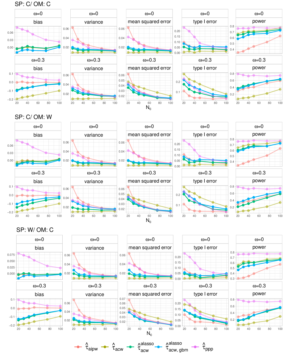
Figure 1: Simulation results under various levels of $\omega$, and different model choices of $q(X)$ and $\mu_{0}(X)$.

Figure 1 displays the average bias, variance, mean squared error, type I error when ${E}\{\tau(X)\mid R=1\}=0$, and power for testing $\tau>0$ when ${E}\{\tau(X)\mid R=1\}=0.3$ based on $1000$ sets of data replications. Over the three model scenarios, $\widehat{\tau}_{{\mathrm{aipw}}}$ is always consistent but lacks efficiency as it only utilizes controls from the RPCT for estimation, especially when $N_{c}$ is small. When the conditional mean exchangeability in Assumption 2 holds (i.e., $\omega=0$), the ACW estimator $\widehat{\tau}_{\mathrm{acw}}$ is most efficient, shown by its low mean squared error and high power for detecting a significant treatment effect. When Assumption 2 is violated (i.e., $\omega=0.3$), $\widehat{\tau}_{\mathrm{acw}}$ becomes biased, leading to inflated type I error and low power. The Bayesian estimator $\widehat{\tau}_{\mathrm{ppp}}$ requires correct parametric specification of the outcome model and performs poorly when the model omits a key confounder that is imbalanced between data sources. In our simulations, high weights were assigned to the external control subjects, which led to some bias in the treatment effect estimates when $N_{c}$ was small. Our proposed estimator $\widehat{\tau}_{\mathrm{acw}}^{\mathrm{alasso}}$ and $\widehat{\tau}_{\mathrm{acw},\mathrm{gbm}}^{\mathrm{alasso}}$ are consistent and achieve improved or comparable power levels compared with $\widehat{\tau}_{{\mathrm{aipw}}}$ over all the model choices regardless of whether Assumption 2 holds or not. In the case where outcome model is not correctly specified and $\omega=0.3$, the benefit of using the machine learning method is highlighted. Particularly, the flexibility of the gradient boosting model guarantees the convergence rate assumption for $\widehat{b}_{i}$, that is, $a_{N}(\widehat{b}_{i}-b_{i,0})=O_{{\mathrm{pr}}}(1)$ for a certain sequence $a_{N}$ (Zhang and Yu, 2005). By correctly filtering out incompatible ECs, $\widehat{\tau}_{\mathrm{acw},\mathrm{gbm}}^{\mathrm{alasso}}$ controls the bias well and achieves comparable power levels as $\widehat{\tau}_{{\mathrm{aipw}}}$. But the adaptive LASSO estimation based on the misspecified linear model lacks such properties, and is therefore subject to inferior powers. One notable trade-off of our proposed estimators is the type I error inflation when $N_{c}$ is small and Assumption 2 is violated, which can be attributed to finite-sample selection uncertainty and is also observed in Viele et al. (2014).

4 Real-data Application

In this section, we present an application of the proposed methodology to investigate the effectiveness of basal Insulin Lispro (BIL) against regular Insulin Glargine (GL) in patients with type I diabetes. An additional real-data application leveraging external real-world observational data to examine the effectiveness of Solanezumab versus placebo to slow the progression of Alzheimer’s Disease is included in Section LABEL:supple-sec:application-II of the Supplemental Material.

When combined with preprandial insulin lispro, BIL and GL are two long-acting Insulin formulations used for patients with Type I diabetes mellitus. We examine a cohort of patients enrolled in the open-label IMAGINE-1 study as the under-powered clinical trial, in which patients were randomized to the treatment group BIL or the control group GL in an imbalanced manner. Meanwhile, the IMAGINE-3 study is another multi-center double-blinded randomized trial that compares BIL to GL, whose control group will be utilized to augment the IMAGINE-1 study. The IMAGINE-3 study is registered at clinicaltrials.gov as NCT01454284 and detailed illustration can be found in Bergenstal et al. (2016).

Our primary objective is to test the hypothesis whether BIL is superior to GL at glycemic control for patients with Type I diabetes mellitus. This can be achieved by comparing the deviation of hemoglobin A1c (HbA1c) level from baseline after 52 weeks of treatment. Both IMAGINE-1 and IMAGINE-3 studies contain a rich set of baseline covariates $X$, such as age, gender, baseline Hemoglobin A1c (%), baseline fasting serum glucose (mmol/L), baseline Triglycerides (mmol/L), baseline low density lipoprotein cholesterol (mmol/L) and baseline Alanine Transaminase (U/L). After removing patients with missing baseline information and adopting the last observation carried forward method to impute missing post-baseline outcomes, the IMAGINE-1 study consists of $N_{\mathcal{R}}=439$ subjects with $286$ in the treated group and $153$ in the control group, while the IMAGINE-3 study includes $N_{\mathcal{E}}=444$ patients on the control arm. Our statistical analysis aims to transport control-group information from the IMAGINE-3 study to the IMAGINE-1 study. First, we use the baseline covariates $X$ to model the trial inclusion probability by calibration weighting under the entropy loss function. Next, we assume a linear heterogeneity treatment effect function for the outcomes with $X$ as the treatment modifier, and compare the same set of estimators in the simulation study.

Table 2 reports the estimated results. The benchmark estimator AIPW shows that BIL has a significant treatment effect on reducing the glucose level solely based on the IMAGINE-1 study. Due to potential population bias, the ACW and PPP estimates for the treatment effects, albeit significant, are slightly different from the AIPW estimator, which may be subject to possible biases of the ECs. After filtering out $12$ incompatible patients from the control group of the IMAGINE-3 study by our adaptive LASSO selection, the final integrative estimate is closer to the AIPW but has a narrower confidence interval. According to our adaptive analysis result, BIL is significantly more effective than regular GL at glycemic control when used for patients with Type I diabetes mellitus.

Table 2: Point estimates, standard errors, and 95% confidence intervals of the treatment effect of BIL against regular GL based on the IMAGINE-1 and IMAGINE-3 studies

	$\widehat{\tau}_{{\mathrm{aipw}}}$	$\widehat{\tau}_{\mathrm{acw}}$	$\widehat{\tau}_{\mathrm{acw}}^{\mathrm{alasso}}$	$\widehat{\tau}_{\mathrm{ppp}}$
Est.	-0.25	-0.22	-0.24	-0.27
S.E.	0.072	0.057	0.065	0.062
C.I.	(-0.39,-0.11)	(-0.33,-0.11)	(-0.37,-0.08)	(-0.39,-0.15)

Next, we focus on comparing the performances of $\widehat{\tau}_{{\mathrm{aipw}}}$ and $\widehat{\tau}_{\mathrm{acw}}^{\mathrm{alasso}}$ to highlight the advantages of our dynamic borrowing framework. To accomplish it, we retain the size of the treatment group but create $100$ sub-samples by randomly selecting $N_{c}^{s}$ patients from its control group, where $N_{c}^{s}=10,15,\cdots,150,153$. Then, the patients treated by regular GL in the IMAGINE-3 study are augmented to each selected sub-sample and the treatment effect is evaluated upon the hybrid control arms design. Figure 2 presents the average probabilities of successfully detecting $\tau<-0.1$, the so-called probability of success, against the size of sub-samples. When solely utilizing patients from the IMAGINE-1 study, the AIPW produces a probability of success larger than $0.8$ only if the size of the control group is larger than $25$. Combined with the IMAGINE-3 study, it refines the treatment effect estimation and only $15$ patients are needed in the concurrent control group to attain a probability of success higher than $0.8$. Therefore, by properly leveraging the ECs, we may accelerate drug development by decreasing the number of patients on the concurrent control, thereby reducing the duration and cost of the clinical trial.

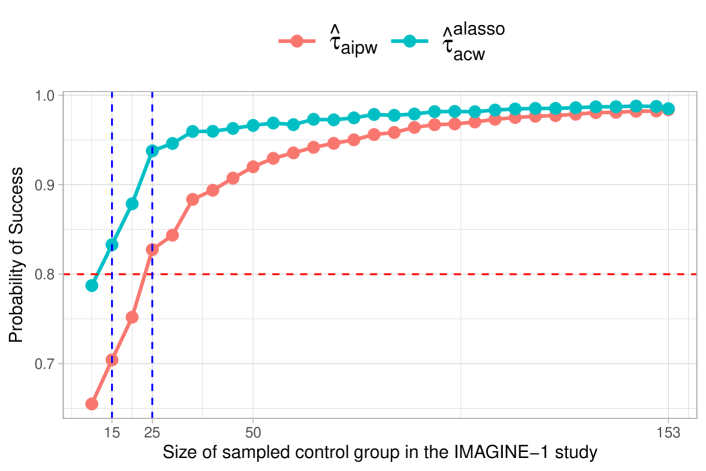
Figure 2: Probability of success for detecting $\tau<-0.1$ by estimators $\widehat{\tau}_{{\mathrm{aipw}}}$ and $\widehat{\tau}_{\mathrm{acw}}^{\mathrm{alasso}}$ with varying control group size of the IMAGINE-1 study; The red dashed line represents the probability $0.8$.

5 Extension to Multiple External Controls

In the previous sections, we illustrate the proposed data-adaptive integrative estimator with only one external group $\mathcal{E}$. In this section, we extend that to the case with multiple external groups, denoted by $\mathcal{E}^{[1]},\cdots,\mathcal{E}^{[K]}$ with size $N_{\mathcal{E}}^{[1]},\cdots,N_{\mathcal{E}}^{[K]}$, respectively. The total sample size now is $N=N_{\mathcal{R}}+\sum_{k=1}^{K}N_{\mathcal{E}}^{[k]}.$ Let $R_{i}^{[k]}$ be the data source indicator for the EC group $\mathcal{E}^{[k]}$. An assumption similar to Assumption 2 is requested when integrating multiple external groups with the concurrent RPCT study.

Assumption 4 (Multiple external controls compatibility).

For any $k=1,\cdots,K$, (i)

$${E}\left\{Y(0)\mid X=x,R_{i}^{[k]}=1\right\}={E}\{Y(0)\mid X=x,R_{i}^{[k]}=0\},$$

and (ii) $P(R^{[k]}=1\mid X=x)>0$ for all $x$ s.t. $P(X=x,R^{[k]}=1)>0$.

In a similar manner, the ACW estimator $\widehat{\tau}_{\mathrm{acw}}^{[k]}$ for combining $\mathcal{E}^{[k]}$ with $\mathcal{R}$ can be rewritten by

$$\widehat{\tau}_{\mathrm{acw}}^{[k]} =\frac{1}{N_{\mathcal{R}}}\sum_{i\in\mathcal{\mathcal{R}}\cup\mathcal{E}^{[k]}}R_{i}^{[k]}\left[\frac{A_{i}\{Y_{i}-\widehat{\mu}_{1}(X_{i})\}}{\pi_{A}(X_{i})}+\widehat{\mu}_{1}(X_{i})-\widehat{\mu}_{0}(X_{i})\right]$$

$$-\frac{1}{N_{\mathcal{R}}}\sum_{i\in\mathcal{\mathcal{R}}\cup\mathcal{E}^{[k]}}\frac{R_{i}^{[k]}(1-A_{i})\widehat{q}^{[k]}(X_{i})+(1-R_{i}^{[k]})\widehat{q}^{[k]}(X_{i})\widehat{r}^{[k]}(X_{i})}{\widehat{r}^{[k]}(X_{i})+\{1-\pi_{A}(X_{i})\}\widehat{q}^{[k]}(X_{i})}\widehat{\epsilon}_{0,i},$$

where $r^{[k]}(X)=\text{var}\{Y(0)\mid X,R^{[k]}=1\}/\text{var}\{Y(0)\mid X,R^{[k]}=0\}$, and $\widehat{q}^{[k]}(X)$ is the estimated calibration weights balancing the covariate distribution in $\mathcal{E}^{[k]}$ to the target RPCT group. As illustrated previously, the conditional mean exchangeability in Assumption 4 might be violated in practice. With slight modification, our proposed method is able to accommodate these potential violations presented in multiple external resources.

Theorem 5.

Let $\widehat{\tau}_{\mathrm{acw}}^{\mathrm{alasso},[1:K]}=(\widehat{\tau}_{\mathrm{acw}}^{\mathrm{alasso},[1]},\cdots,\widehat{\tau}_{\mathrm{acw}}^{\mathrm{alasso},[K]})^{\intercal}$ be the concatenated data-adaptive ACW estimators for $K$ external groups, we have $N^{1/2}(\widehat{\tau}_{\mathrm{acw}}^{\mathrm{alasso},[1:K]}-\tau)\rightarrow\mathcal{N}(\bm{0}_{K},\Sigma_{\tau}^{\mathrm{alasso}})$. Thus, the final integrative estimator is $\widehat{\tau}_{\mathrm{acw}}^{\mathrm{*}}=\bm{\widehat{d}}^{\intercal}\widehat{\tau}_{\mathrm{acw}}^{\mathrm{alasso},[1:K]}\rightarrow\mathcal{N}(0,\bm{\widehat{d}}^{\intercal}\Sigma_{\tau}^{\mathrm{alasso}}\bm{\widehat{d}})$, where $\bm{\widehat{d}}=\left\{\mathbf{1}_{K}^{\intercal}(\Sigma_{\tau}^{\mathrm{alasso}})^{-1}\mathbf{1}_{K}\right\}^{-1}(\Sigma_{\tau}^{\mathrm{alasso}})^{-1}\mathbf{1}_{K}$.

More details of Theorem 5 are presented in Section LABEL:supple-subsec:proof-multiple-HCs of the Supplementary Material. The reason that we do not treat the multiple EC groups as one entity is due to the fact that different external resources might possess different covariate distributions since they can be collected by various registry databases. Therefore, it is optimal to calibrate each EC group individually to the RPCT data for reaching stable weight estimation.

6 Discussion

The use of external control arms in drug development is becoming more prevalent, but the concerns regarding their quality and validity severely restrict their application in practice, which requires careful and appropriate assessment. In this paper, a data-driven adaptive borrowing hinged on penalized estimation is proposed to accommodate subject-level disparity of the external resources. Our penalized estimation is based on the adaptive LASSO penalty, but alternative penalties can also be considered as long as the selection consistency property is attained. One well-known example can be the smoothly clipped absolute deviation (SCAD) penalty (Fan and Li, 2001), which is widely used in the variable selection literature.

In our real-data-informed simulation studies, the proposed estimator is able to achieve promising performance for point estimation under correct model specification. By leveraging the off-the-shelf machine learning methods, we achieve the consistent selection of compatible ECs, and improved performance is observed over the RPCT-only estimator. As for the confidence intervals, our proposed estimator may slightly suffer type I error inflation when the data is subject to unmeasured confounders, which is also noted when Bayesian dynamic borrowing is implemented to integrate external resources (Dejardin et al., 2018; Kopp-Schneider et al., 2020). This behavior becomes more pronounced when the sample size of the concurrent control group is small, which can be attributed to the selection uncertainty in finite samples. One future work direction will be rigorously constructing a data-adaptive confidence interval to account for the finite-sample selection uncertainty while refraining being overly conservative. In addition, the proposed integrated inferential framework can also be extended to survival outcomes (Lee et al., 2022b), heterogeneity of treatment effects learning (Wu and Yang, 2022a; Yang et al., 2022) and combining probability and non-probability samples (Yang et al., 2020; Gao and Yang, 2023), which will be studied in the future.

References

- (1)
- Bergenstal et al. (2016) Bergenstal, R., Lunt, H., Franek, E., Travert, F., Mou, J., Qu, Y., Antalis, C., Hartman, M., Rosilio, M., Jacober, S. et al. (2016). Randomized, double-blind clinical trial comparing basal insulin peglispro and insulin glargine, in combination with prandial insulin lispro, in patients with type 1 diabetes: Imagine 3, Diabetes, Obesity and Metabolism 18(11): 1081–1088.
- Bickel et al. (1998) Bickel, P. J., Klaassen, C., Ritov, Y. and Wellner, J. (1998). Efficient and adaptive inference in semiparametric models.
- Cao et al. (2009) Cao, W., Tsiatis, A. A. and Davidian, M. (2009). Improving efficiency and robustness of the doubly robust estimator for a population mean with incomplete data, Biometrika 96: 723–734.
- Chatterjee et al. (2016) Chatterjee, N., Chen, Y.-H., Maas, P. and Carroll, R. J. (2016). Constrained maximum likelihood estimation for model calibration using summary-level information from external big data sources, Journal of the American Statistical Association 111: 107–117.
- Chen (2007) Chen, X. (2007). Large sample sieve estimation of semi-nonparametric models, Handbook of Econometrics 6: 5549–5632.
- Chen et al. (2021) Chen, Z., Ning, J., Shen, Y. and Qin, J. (2021). Combining primary cohort data with external aggregate information without assuming comparability, Biometrics 77: 1024–1036.
- Chernozhukov et al. (2018) Chernozhukov, V., Chetverikov, D., Demirer, M., Duflo, E., Hansen, C., Newey, W. and Robins, J. (2018). Double/debiased machine learning for treatment and structural parameters, The Econometrics Journal 21: 1–68.
- Chu et al. (2022) Chu, J., Lu, W. and Yang, S. (2022). Targeted optimal treatment regime learning using summary statistics, arXiv:2201.06229 .
- Colnet et al. (2020) Colnet, B., Mayer, I., Chen, G., Dieng, A., Li, R., Varoquaux, G., Vert, J.-P., Josse, J. and Yang, S. (2020). Causal inference methods for combining randomized trials and observational studies: a review, arXiv:2011.08047 .
- Dejardin et al. (2018) Dejardin, D., Delmar, P., Warne, C., Patel, K., van Rosmalen, J. and Lesaffre, E. (2018). Use of a historical control group in a noninferiority trial assessing a new antibacterial treatment: A case study and discussion of practical implementation aspects, Pharmaceutical Statistics 17: 169–181.
- Fan and Li (2001) Fan, J. and Li, R. (2001). Variable selection via nonconcave penalized likelihood and its oracle properties, Journal of the American statistical Association 96: 1348–1360.
- Food and Drug Administration (2001) Food and Drug Administration (2001). E10 choice of control group and related issues in clinical trials, https://www.fda.gov/media/71349/download. Accessed: 2023-02-23.
- Food and Drug Administration (2014) Food and Drug Administration (2014). Blinatumomab drug approval package. Accessed: 2023-02-23.
- Food and Drug Administration (2016) Food and Drug Administration (2016). Avelumab drug approval package. Accessed: 2023-02-23.
- Food and Drug Administration (2019) Food and Drug Administration (2019). Rare diseases: Natural history studies for drug development, https://www.fda.gov/media/122425/download. Accessed: 2023-02-23.
- Food and Drug Administration (2021) Food and Drug Administration (2021). Real-world data: Assessing registries to support regulatory decision-making for drug and biological products guidance for industry, https://www.fda.gov/media/154449/download. Accessed: 2023-02-23.
- Food and Drug Administration (2023) Food and Drug Administration (2023). Considerations for the design and conduct of externally controlled trials for drug and biological products guidance for industry, https://www.fda.gov/media/164960/download. Accessed: 2023-02-23.
- Gao and Yang (2023) Gao, C. and Yang, S. (2023). Pretest estimation in combining probability and non-probability samples, Electronic Journal of Statistics 17: 1492–1546.
- Ghadessi et al. (2020) Ghadessi, M., Tang, R., Zhou, J., Liu, R., Wang, C., Toyoizumi, K., Mei, C., Zhang, L., Deng, C. and Beckman, R. A. (2020). A roadmap to using historical controls in clinical trials–by drug information association adaptive design scientific working group (dia-adswg), Orphanet Journal of Rare Diseases 15: 1–19.
- Ho et al. (2007) Ho, D. E., Imai, K., King, G. and Stuart, E. A. (2007). Matching as nonparametric preprocessing for reducing model dependence in parametric causal inference, Political Analysis 15: 199–236.
- Hobbs et al. (2011) Hobbs, B. P., Carlin, B. P., Mandrekar, S. J. and Sargent, D. J. (2011). Hierarchical commensurate and power prior models for adaptive incorporation of historical information in clinical trials, Biometrics 67: 1047–1056.
- Ibrahim and Chen (2000) Ibrahim, J. G. and Chen, M.-H. (2000). Power prior distributions for regression models, Statistical Science 15: 46–60.
- Imbens (2004) Imbens, G. W. (2004). Nonparametric estimation of average treatment effects under exogeneity: A review, Review of Economics and Statistics 86: 4–29.
- Kopp-Schneider et al. (2020) Kopp-Schneider, A., Calderazzo, S. and Wiesenfarth, M. (2020). Power gains by using external information in clinical trials are typically not possible when requiring strict type i error control, Biometrical Journal 62: 361–374.
- Kwiatkowski et al. (2023) Kwiatkowski, E., Zhu, J., Li, X., Pang, H., Lieberman, G. and Psioda, M. A. (2023). Case weighted adaptive power priors for hybrid control analyses with time-to-event data, arXiv preprint arXiv:2305.05913 .
- Lee et al. (2022) Lee, D., Yang, S., Dong, L., Wang, X., Zeng, D. and Cai, J. (2022). Improving trial generalizability using observational studies, Biometrics 79: 1213–1225.
- Lee et al. (2022b) Lee, D., Yang, S. and Wang, X. (2022b). Doubly robust estimators for generalizing treatment effects on survival outcomes from randomized controlled trials to a target population, Journal of Causal Inference 10: 415–440.
- Li et al. (2021) Li, X., Miao, W., Lu, F. and Zhou, X.-H. (2021). Improving efficiency of inference in clinical trials with external control data, Biometrics .
- Liu et al. (2021) Liu, M., Bunn, V., Hupf, B., Lin, J. and Lin, J. (2021). Propensity-score-based meta-analytic predictive prior for incorporating real-world and historical data, Statistics in Medicine 40: 4794–4808.
- Neuenschwander et al. (2009) Neuenschwander, B., Branson, M. and Spiegelhalter, D. J. (2009). A note on the power prior, Statistics in Medicine 28: 3562–3566.
- Neuenschwander et al. (2010) Neuenschwander, B., Capkun-Niggli, G., Branson, M. and Spiegelhalter, D. J. (2010). Summarizing historical information on controls in clinical trials, Clinical Trials 7: 5–18.
- Odogwu et al. (2018) Odogwu, L., Mathieu, L., Blumenthal, G., Larkins, E., Goldberg, K. B., Griffin, N., Bijwaard, K., Lee, E. Y., Philip, R., Jiang, X., Rodriguez, L., McKee, A. E., Keegan, P. and Pazdur, R. (2018). Fda approval summary: Dabrafenib and trametinib for the treatment of metastatic non-small cell lung cancers harboring braf v600e mutations, The Oncologist 23: 740–745.
- Phelan et al. (2017) Phelan, M., Bhavsar, N. A. and Goldstein, B. A. (2017). Illustrating informed presence bias in electronic health records data: how patient interactions with a health system can impact inference, Journal for Electronic Health Data and Methods 5.
- Pocock (1976) Pocock, S. J. (1976). The combination of randomized and historical controls in clinical trials, Journal of Chronic Diseases 29: 175–188.
- Qin et al. (2015) Qin, J., Zhang, H., Li, P., Albanes, D. and Yu, K. (2015). Using covariate-specific disease prevalence information to increase the power of case-control studies, Biometrika 102(1): 169–180.
- Rosenbaum and Rubin (1983a) Rosenbaum, P. R. and Rubin, D. B. (1983a). The central role of the propensity score in observational studies for causal effects, Biometrika 70: 41–55.
- Rosenbaum and Rubin (1983b) Rosenbaum, P. R. and Rubin, D. B. (1983b). The central role of the propensity score in observational studies for causal effects, Biometrika 70(1): 41–55.
- Rubin (1974) Rubin, D. B. (1974). Estimating causal effects of treatments in randomized and nonrandomized studies., Journal of educational Psychology 66(5): 688.
- Schoenfeld et al. (2019) Schoenfeld, D. A., Finkelstein, D. M., Macklin, E., Zach, N., Ennist, D. L., Taylor, A. A., Atassi, N. and Consortium, P. R. O.-A. A. C. T. (2019). Design and analysis of a clinical trial using previous trials as historical control, Clinical Trials 16: 531–538.
- Shan et al. (2022) Shan, M., Faries, D., Dang, A., Zhang, X., Cui, Z. and Sheffield, K. M. (2022). A simulation-based evaluation of statistical methods for hybrid real-world control arms in clinical trials, Statistics in Biosciences 14: 259–284.
- Silverman (2018) Silverman, B. (2018). A baker’s dozen of US FDA efficacy approvals using real world evidence, Pharma Intelligence Pink Sheet .
- Stuart (2010) Stuart, E. A. (2010). Matching methods for causal inference: A review and a look forward, Statistical Ccience: a review Journal of the Institute of Mathematical Statistics 25: 1.
- Stuart and Rubin (2008) Stuart, E. A. and Rubin, D. B. (2008). Matching with multiple control groups with adjustment for group differences, Journal of Educational and Behavioral Statistics 33: 279–306.
- Tsiatis (2006) Tsiatis, A. (2006). Semiparametric Theory and Missing Data, Springer, New York.
- Van der Vaart (2000) Van der Vaart, A. W. (2000). Asymptotic statistics, Vol. 3, Cambridge university press.
- van Rosmalen et al. (2018) van Rosmalen, J., Dejardin, D., van Norden, Y., Löwenberg, B. and Lesaffre, E. (2018). Including historical data in the analysis of clinical trials: Is it worth the effort?, Statistical Methods in Medical Research 27: 3167–3182.
- Viele et al. (2014) Viele, K., Berry, S., Neuenschwander, B., Amzal, B., Chen, F., Enas, N., Hobbs, B., Ibrahim, J. G., Kinnersley, N., Lindborg, S. et al. (2014). Use of historical control data for assessing treatment effects in clinical trials, Pharmaceutical statistics 13(1): 41–54.
- Visvanathan et al. (2017) Visvanathan, K., Levit, L. A., Raghavan, D., Hudis, C. A., Wong, S., Dueck, A. and Lyman, G. H. (2017). Untapped potential of observational research to inform clinical decision making: American Society of Clinical Oncology research statement, Journal of Clinical Oncology 35: 1845–1854.
- Wager and Athey (2018) Wager, S. and Athey, S. (2018). Estimation and inference of heterogeneous treatment effects using random forests, Journal of the American Statistical Association 113: 1228–1242.
- Wu and Yang (2022a) Wu, L. and Yang, S. (2022a). Integrative -learner of heterogeneous treatment effects combining experimental and observational studies, Conference on Causal Learning and Reasoning, PMLR, pp. 904–926.
- Wu and Yang (2022b) Wu, L. and Yang, S. (2022b). Transfer learning of individualized treatment rules from experimental to real-world data, Journal of Computational and Graphical Statistics pp. 1–10.
- Yang et al. (2020) Yang, S., Kim, J. K. and Song, R. (2020). Doubly robust inference when combining probability and non-probability samples with high dimensional data, Journal of the Royal Statistical Society. Series B, Statistical Methodology 82: 445.
- Yang et al. (2022) Yang, S., Zeng, D. and Wang, X. (2022). Elastic integrative analysis of randomized trial and real-world data for treatment heterogeneity estimation, arXiv:2005.10579 .
- Zhai and Han (2022) Zhai, Y. and Han, P. (2022). Data integration with oracle use of external information from heterogeneous populations, Journal of Computational and Graphical Statistics 31: 1001–1012.
- Zhang et al. (2020) Zhang, H., Deng, L., Schiffman, M., Qin, J. and Yu, K. (2020). Generalized integration model for improved statistical inference by leveraging external summary data, Biometrika 107: 689–703.
- Zhang and Yu (2005) Zhang, T. and Yu, B. (2005). Boosting with early stopping: Convergence and consistency, The Annals of Statistics 33: 1538–1579.
- Zou (2006) Zou, H. (2006). The adaptive LASSO and its oracle properties, Journal of the American Statistical Association 101: 1418–1429.