GuidedMixup: An Efficient Mixup Strategy Guided by Saliency Maps

Abstract

Data augmentation is now an essential part of the image training process, as it effectively prevents overfitting and makes the model more robust against noisy datasets. Recent mixing augmentation strategies have advanced to generate the mixup mask that can enrich the saliency information, which is a supervisory signal. However, these methods incur a significant computational burden to optimize the mixup mask. From this motivation, we propose a novel saliency-aware mixup method, GuidedMixup, which aims to retain the salient regions in mixup images with low computational overhead. We develop an efficient pairing algorithm that pursues to minimize the conflict of salient regions of paired images and achieve rich saliency in mixup images. Moreover, GuidedMixup controls the mixup ratio for each pixel to better preserve the salient region by interpolating two paired images smoothly. The experiments on several datasets demonstrate that GuidedMixup provides a good trade-off between augmentation overhead and generalization performance on classification datasets. In addition, our method shows good performance in experiments with corrupted or reduced datasets.

1 Introduction

Improvement and success of deep neural networks have been achieved in various tasks by employing more parameters and larger architectures. However, compared to the capacity increase of deep neural networks, the number of samples in datasets has not kept up. The capacity increase can incur the memorization effect, which appears as an overfitting phenomenon to training data (Srivastava et al. 2014) and vulnerability to noisy data.

In order to tackle these issues, many regularization methods have been studied (Srivastava et al. 2014; Huang et al. 2016). In particular, data augmentation (Krizhevsky, Sutskever, and Hinton 2012; DeVries and Taylor 2017) can effectively regularize the model independently and is now a crucial part of training. The primary purpose of augmentation is to improve the model’s generalization ability by generating appropriate unseen data without additional datasets. Recently, a body of research has attempted to develop mixing augmentation techniques. For example, Zhang et al. (2018) proposed Mixup, which linearly interpolates images to address the issues of generalization and robustness (Stanton et al. 2021). Yun et al. (2019) proposed CutMix that replaces a random-sized patch of the source image with the same-sized region of the target image.

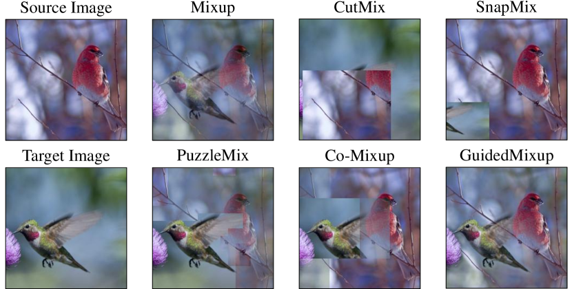
Figure 1: The generated images of previous mixup augmentation methods and the proposed GuidedMixup.

These mixup strategies have improved generalization and robustness with lower computational costs. However, as shown in Figure 1, these approaches have limitations in containing enough saliency information (i.e., a supervisory signal). In order to address this issue, there has been another line of studies on properly assigning the saliency information from each image to the mixup images (Kim, Choo, and Song 2020; Kim et al. 2020). PuzzleMix (Kim, Choo, and Song 2020) argued how to generate the mixup mask and optimally transport guided by saliency information. While PuzzleMix rearranges the salient region to the proper location for obtaining maximum saliency, Co-Mixup (Kim et al. 2020) finds the optimal pairs and generates the optimal masks simultaneously from the input batch by solving an optimization problem. With the optimal pairs, Co-Mixup was able to obtain richer saliency information in an image than PuzzleMix without the rearrangement. However, saliency-based mixup strategies require a non-trivial computational cost to achieve optimal performance. Furthermore, as the computational inefficiency increases with larger mini-batch, the option of large mini-batch size can be restricted, which may have an optimal point.

In this regard, we propose GuidedMixup, which achieves both computational efficiency and effective performance by searching the pairs and mixup masks within the input batch. We first formulate a novel pairing optimization problem to minimize the conflict of each salient region in mixup images. Unfortunately, this problem results in a graph-matching problem with higher complexity. To efficiently reduce the complexity, we introduce a greedy pairing algorithm to find the best sets with a large distance between salient regions among the mini-batch images.

The efficiency of our paring algorithm brings about high flexibility in the choice of the mask unit size. This is in contrast to previous approaches that are limited to using a large block size due to computational cost. Accordingly, we suggest a mixup mask generation algorithm that maximally leverages saliency information for each pixel and adjusts the mixing ratio pixel by pixel. This can better preserve salient regions of each image within the mixup image and interpolate two images smoothly, which leads to robustness improvement. Figure 1 shows the comparison between previous methods and ours.

In the extensive experiments, GuidedMixup non-trivially improves the generalization performance on CIFAR-100 and Tiny-ImageNet. The outperforming results on fine-grained datasets indicate that GuidedMixup can effectively mix images while maintaining the fine details of original images. To validate the efficiency of GuidedMixup, we measure the computational overhead of mixup strategies. We find that GuidedMixup provides good trade-offs between augmentation overhead and generalization performance. Furthermore, since the main purpose of augmentation is to handle overfitting and robustness, we validate our method under the condition of data scarcity and corruption.

2 Related Work

Augmentation is one of the regularization methods to address the overfitting problem caused by the gap between the increased capacity and the number of data that is less increased as the model develops. It increases the number of data that gives the diversity of data through various transformations. The most frequently used techniques are horizontal flipping or random cropping (Krizhevsky, Sutskever, and Hinton 2012). Through this, Bishop (1995) has focused on creating a vicinity of a given dataset to improve generalization performance. Bishop and Nasrabadi (2006) also applied a method of giving occlusion to the image by applying various noises or smoothing. In addition to such direct design augmentation, Lemley, Bazrafkan, and Corcoran (2017) proposed an end-to-end augmentation process, which is Smart Augmentation, that learns an augmentation process consisting of a serial combination of multiple affine transforms. Hendrycks et al. (2020) proposed AugMix, which interpolates multiple warping augmentation techniques to improve the robustness of the neural network and prevent overfitting.

Compared to data-warping augmentation, the other line of augmentation, which is the mixup-based method, has recently been proposed. Zhang et al. (2018) proposed the method named ‘MixUp,’ which creates linearly interpolated virtual training examples with a random mixing ratio. Mixup leads the model to have smoother decision boundaries and ameliorates the robustness against noise data (Stanton et al. 2021). Verma et al. (2019) proposed an extended version of Mixup named Manifold Mixup, which interpolates data at the feature level. Also, Yun et al. (2019) suggested CutMix, which replaces a randomly generated spatial patch of the input with another and assigns an area ratio label that is irrelevant to the actual information in the mixed data. SaliencyMix (Uddin et al. 2020) proposed a CutMix-based method so that a random-sized patch is cut from the most salient point in an image.

The randomness in existing methods may generate improper samples, resulting in misleading models. For this reason, generating images appropriate for the model has become mainstream research. SnapMix (Huang, Wang, and Tao 2021) proposed the idea of asymmetrically replacing the random size patch of an image with another by utilizing a class activation map (CAM) (Zhou et al. 2016) as the guidance of a semantic label. PuzzleMix (Kim, Choo, and Song 2020) also proposes a mixup method that transports rich salient information to another image by solving the optimization problem. Kim et al. (2020) proposed Co-MixUp, which finds the proper combination of salient regions and pairs simultaneously from the optimal solution of optimization problems.

“Saliency object detection” was first suggested by Itti, Koch, and Niebur (1998), who integrated two separate stages that are 1) distinguishing the most salient object from the background (detecting) and 2) segmenting the specific region of the object (segmenting). We roughly categorize saliency object detection methods in two ways, whether utilizing the neural network or not. Achanta et al. (2009) proposed the detection methods that use frequency domain without the neural network. Hou and Zhang (2007) proposed a spectral residual approach that utilizes conventional signal processing theory to distinguish the objects by approximating background statistics. On the contrary, Simonyan, Vedaldi, and Zisserman (2013) proposed the method that generates a saliency map by using the computed gradients from the pre-trained model. Zhao et al. (2015) proposed the method to precisely generate the saliency map by simultaneously combining global and local contexts from the pre-trained model.

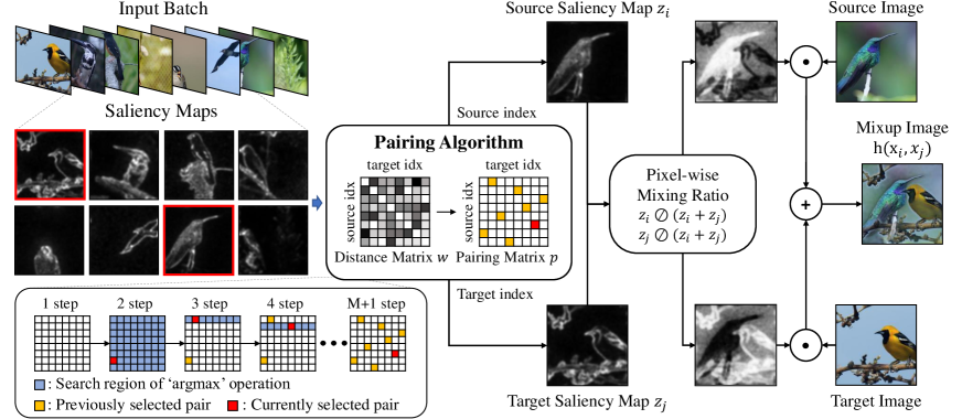
Figure 2: An overall diagram of GuidedMixup. GuidedMixup augmentation pipeline consists of the following 4 steps: 1) Generate saliency maps from mini-batch images. 2) Construct a pairing matrix $p$ from the distance matrix $w$ by utilizing pairing algorithm. 3) To obtain mixup masks, adjust the pixel-wise mixing ratio between each pixel in the source and target saliency map. 4) Final mixup images are obtained as the pixel-wise sum of masked images.

3 Preliminary

Mixing data augmentation methods generate synthetic data $\hat{x}$ and the corresponding label $\hat{y}$ from a given mixup function $\hat{x}=h(x_{s},x_{t})$, where $x_{s},x_{t}\in\mathbb{R}^{N}$ are the source and target image, respectively.

For example, in the case of input mixup, $h(x_{s},x_{t})=\lambda x_{s}+(1-\lambda)x_{t}$. CutMix uses $h(x_{s},x_{t})=z\odot x_{s}+(1-z)\odot x_{t}$, where $z\in{\{0,1\}}^{N}$ is a binary rectangular-shaped mask which has the same shape of target image $x_{t}\in N$ and $\odot$ represents the point-wise multiplication. SaliencyMix uses the same function as CutMix but obtains the location of the rectangular-shaped mask from the maximum point of a saliency map. PuzzleMix uses $h(x_{s},x_{t})=z\odot\Pi^{\top}_{s}x_{s}+(1-z)\odot\Pi^{\top}_{t}x_{t}$ where $\Pi$ is a transport mask and $z$ is a discrete saliency-based mask.

For mini-batch size input, a mixup function can be described as the following: $\hat{x}_{B}=H(x_{B})$. Co-Mixup uses $H(x_{B})=\{g(z_{m}\odot x_{B})|m\in B\}$, where $x_{B}$ is a set of images which have mini-batch size $M$ and $z_{m}\in\mathbb{R}^{M\times N}$ is the mask that makes a pair and augments simultaneously. $g$ is a function $\mathbb{R}^{M\times N}\rightarrow\mathbb{R}^{N}$ that conducts the column-wise summation.

4 Method

The central idea of GuidedMixup is to preserve the object’s shape as much as possible by maintaining the saliency regions in the mixed images through the pairing method and pixel-wise mixing ratio. A recent study (Kim et al. 2020) tries to solve the optimization of mix-matching the inputs to have the maximized saliency measure. As a result, time complexity becomes a burden, which is considering pairs and block-based mask generation simultaneously.

In order to reduce this overhead, we split the augmentation process into two, pairing algorithm and mixup mask generation, which are both guided by saliency information. In solving an optimization problem, this division reduces the number of inputs that increases complexity, such as the batch size of images and the size of the saliency map. The overall diagram is illustrated in Figure 2. In the following sections, we provide a brief background and introduce our GuidedMixup method in detail.

4.1 Pairing Algorithm

The pairing algorithm in GuidedMixup pursues to let the mixup images embrace the salient regions unperturbed as much as possible. The main objective of the pairing algorithm is to choose source and target pairs towards maximizing the saliency measure by the minimum overlap of salient regions from the mini-batch.

To obtain pairs guided by saliency maps, we conduct the Gaussian-blur on the saliency map $s(x_{k})$ to cover the object well. After Gaussian-blurring the saliency map, we conduct the sum-to-1 normalization $z_{k,i}=s(x_{k,i})/\sum_{n=1}^{N}{s(x_{k,n})}$ to prevent the masks from being biased to the specific images having large salient regions. This can lead to fairly defining the relationship between inputs for matching pairs. As a metric of pair compatibility, we utilize the $\ell_{2}$ distance between saliency maps $z_{k}$. Maximizing the distance between the selected pairs corresponds to minimizing the overlap of salient regions and rich supervisory signals in mixup images. To achieve this, we first calculate a matrix $w\in\mathbb{R}^{M\times M}$ that contains the $\ell_{2}$ distance of each saliency map pair. And then, we find a pairing matrix $p\in\{0,1\}^{M\times M}$ that maximizes the summation of the element-wise multiplication between the distance matrix $w$ and the pairing matrix $p$. The problem can be formulated as follows:

maximize $${\sum_{(i,j)\in B\times B}{w_{i,j}p_{i,j}}},$$ (1)

subject to $${\sum_{i\in B}{p_{i,j}}}=1,$$

$${\sum_{j\in B}{p_{i,j}}}=1,$$

$$p_{i,j}+p_{j,i}\leq 1\quad i,j\in B,$$

$$p_{i,j}=0\quad\text{if }i=j,\quad i,j\in B.$$

All the constraints are diversity terms. The first and second constraints ensure that an image is selected only once as a source or target. The third constraint prevents a symmetric pair $(j,i)$ from being selected when a pair $(i,j)$ is already selected. The fourth constraint avoids an image being paired with itself.

This optimization problem reduces to a Maximum weight $k$-cycle cover in a complete graph, where $k$ is the number of cycles linked to at least three vertices. We can optimally solve this problem in polynomial time by a maximum matching algorithm (Edmonds 1965) through Tutte’s reduction (Tutte 1954). However, the algorithm requires high complexity O($M^{3}$) and can be solved only when the edge weight is an integer to conduct graph reduction. Moreover, since the value of $\ell_{2}$ distance is a real number, mapping to a proper integer can be costly.

As an efficient way to find a satisfactory solution, we propose a greedy algorithm to solve Equation 1, described in Algorithm 1. The algorithm draws one cycle cover in a graph by greedily proceeding to the best remaining neighbor at each vertex. It first selects the largest distance from the distance matrix $w$, then selects the largest from the row corresponding to the target index used as the source in turn while satisfying the constraints. The time complexity is O($M^{2}$), which comes from both finding the first maximum and the loop with the ‘argmax’ operation.

Since the algorithm pairs minimally conflicting images, the proposed pairing algorithm can be applied to other mixup methods. In Section 5.6, we discuss the impact of our pairing algorithm on other mixup baselines.

Algorithm 1 Greedy Pairing Algorithm

0:  distance matrix $w\in\mathbb{R}^{M\times M}$ and batch size $M$

0:  pairing matrix $p\in{\{0,1\}}^{M\times M}$

1:  Initialize $p$ as an $M\times M$ zero matrix

2:  $(i,j)$ = $\underset{i,j}{\text{argmax}}\quad w$

3:  Set $p_{i,j}$ as $1$, and $i$ as $i_{\text{first}}$

4:  Set $w_{k,i}$ = $0$, for all $k\in\{0,...,M-1\}$

5:  for $k=1$ to $M-2$ do

6:     $i$ $\leftarrow$ $j$

7:     $j$ = $\text{argmax}\quad w_{i,:}$

8:     Set $p_{i,j}$ as $1$

9:     Set $w_{k,i}$ = $0$, for all $k\in\{0,...,M-1\}$

10:  end for

11:  Set $p_{j,i_{\text{first}}}$ as $1$

4.2 Masking Algorithm

To keep the salient regions in the mixup image, we use the following algorithm to generate the mask after finding the best pairs among mini-batch. Since the sum-to-1 normalized saliency values $z_{k}$ are too small in each pixel to be used as a mask, the pixel values of mixed images may abnormally decrease when they are directly multiplied by the original image as a mask. To prevent this, we adjust the pixel-wise mixing ratio of each pixel by dividing the saliency map by the sum of the source and target saliency map, denoted as $\oslash$. With the pixel-wise mixing ratio, a mask can be assigned appropriately from both the source and target saliency map that the pixels are desired to highlight. In other words, each pixel in the source saliency map will have high expressive power in the mixed images when it is larger than the corresponding pixel in the target saliency map. Comparing saliency maps in a pixel-wise manner can lead to the salient region being highlighted, as shown in Figure 2. The following Mixup equation is the function of adjusting the pixel-wise mixing ratio matrix between source and target masks.

$$h(x_{s},x_{t})={z_{s}}\oslash{(z_{s}+z_{t})}\odot x_{s}+{z_{t}}\oslash{(z_{s}+z_{t})}\odot x_{t},$$ (2)

where $z_{s},z_{t}\in\mathbb{R}^{N}$ are sum-to-1 normalized saliency maps. Given input $x_{s}$ and $x_{t}$, our mixup function determines the final mixup masks that are generated by utilizing pixel-wise mixing ratio determination between two sum-to-1 normalized saliency maps $z_{t}$ and $z_{s}$. Given mixup masks, the ground-truth of a mixed image $\hat{y}$ is determined as below:

$$\hat{y}_{(s,t)}=\frac{1}{N}\sum_{k\in N}{\frac{z_{s,k}}{z_{s,k}+z_{t,k}}}y_{s}+\frac{1}{N}\sum_{k\in N}{\frac{z_{t,k}}{z_{s,k}+z_{t,k}}}y_{t}.$$ (3)

Finally, with the pairing matrix $p$ from Section 4.1 and the input batch $x_{B}$ as an input of mixup function, we can reformulate Equation 2 to our final mixup function as below:

$$h(x_{B})= {z_{B}}\oslash{(z_{B}+p^{\top}z_{B})}\odot x_{B}$$ (4)

$$+{p^{\top}z_{B}}\oslash{(z_{B}+p^{\top}z_{B})}\odot p^{\top}x_{B}.$$

In summary, our framework is two-fold. First, we determine the pairs following the proposed pairing algorithm with a given batch. Second, after the blur and normalization to the saliency maps, we generate mixup images by linearly interpolating original images weighted by mixup masks, which are pixel-wise mixing ratio matrices.

5 Experiments

In this section, we evaluate the performance and efficiency of GuidedMixup. First, we compare the generalization performance of the proposed method against baselines by training classifiers on CIFAR-100 (Krizhevsky 2009), Tiny-ImageNet (Chrabaszcz, Loshchilov, and Hutter 2017), and ImageNet (Deng et al. 2009) datasets. To validate a broader impact on the generalization, we also measure the performance of four Fine-Grained Vision Classification (FGVC) datasets, which are Caltech-UCSD Birds-200-2011 (CUB) (Wah et al. 2011), Stanford Cars (Cars) (Krause et al. 2013), FGVC-Aircraft (Aircraft) (Maji et al. 2013), and Caltech-101 (Caltech) (Fei-Fei, Fergus, and Perona 2006). To demonstrate the efficiency of our method, we measure the augmentation overhead of all the mixup strategies and examine the generalization performance and overhead simultaneously. Furthermore, we show that our proposed method can improve the performance and robustness simultaneously with AugMix (Hendrycks et al. 2020), which is proposed to improve robustness and uncertainty.

Method	CIFAR-100		Tiny-ImageNet
	Top-1	Top-5	Top-1	Top-5
	Err (%)	Err (%)	Err (%)	Err (%)
Vanilla	23.67	8.98	42.77	26.35
Input Mixup	23.16	7.58	43.41	26.98
Manifold Mixup	20.98	6.63	41.99	25.88
CutMix	23.20	8.09	43.33	26.41
AugMix	24.69	8.38	44.03	25.32
SaliencyMix $\ddagger$	20.25	5.29	43.46	23.86
Guided-SR	19.40	6.00	40.56	23.46
PuzzleMix	19.62	5.85	36.52	24.48
Co-Mixup $\dagger$	19.85	-	35.85	-
Guided-AP	18.80	5.12	35.37	17.51

Table 1: Top-1 / Top-5 error rates (%, $\downarrow$) using PreActResNet-18 on CIFAR-100, and Tiny-ImageNet. The results of Co-Mixup$\dagger$ are from Kim et al. (2020). We reproduce the results of SaliencyMix$\ddagger$. The rest are reported on PuzzleMix (Kim, Choo, and Song 2020).

5.1 Implementation Details

GuidedMixup can be used with any saliency detection method. In this paper, we evaluate our method with two saliency detection approaches; a spectral residual approach for efficiency (Hou and Zhang 2007) and another approach (Simonyan, Vedaldi, and Zisserman 2013), for a fair comparison with Kim, Choo, and Song (2020); Kim et al. (2020), which requires higher complexity due to additional forward and backward passes to obtain precise saliency. We denote GuidedMixup using each saliency detection method as Guided-SR and Guided-AP. After the saliency detection, we employ Gaussian blur to obtain a saliency map that covers the salient region well. We use kernel size as 7 and the sigma of Gaussian distribution as $\sigma$=3 in both our methods.

We categorize all the mixup strategies into two groups: whether requiring additional propagation of model in mixup strategies or not. One group is SnapMix, PuzzleMix, Co-Mixup, and Guided-AP, which require higher computational costs, and all the other mixup methods belong to the other group in the following experiments. Note that SnapMix utilizes class activation map (Zhou et al. 2016) as a saliency detection method, which requires only a forward pass. The other mixup methods in the group requiring additional propagation utilize Simonyan, Vedaldi, and Zisserman (2013), which requires both forward and backward passes.

5.2 Generalization Performance on General Classification Datasets

To validate the generalization performance of our GuidedMixup, we first train and evaluate the model on classification datasets such as CIFAR-100, Tiny-ImageNet, and ImageNet. First, we evaluate our method on CIFAR-100 and Tiny-ImageNet with a residual network model (PreActResNet-18) (He et al. 2016b) following the protocol of Verma et al. (2019). As shown in Table 1, we observe that Guided-SR outperforms the other augmentation baselines among the group, which does not require additional network propagations. Guided-AP also achieves the best performance in generalization on CIFAR-100 and Tiny-ImageNet among all the mixup strategies. ImageNet will be discussed in Section 5.5.

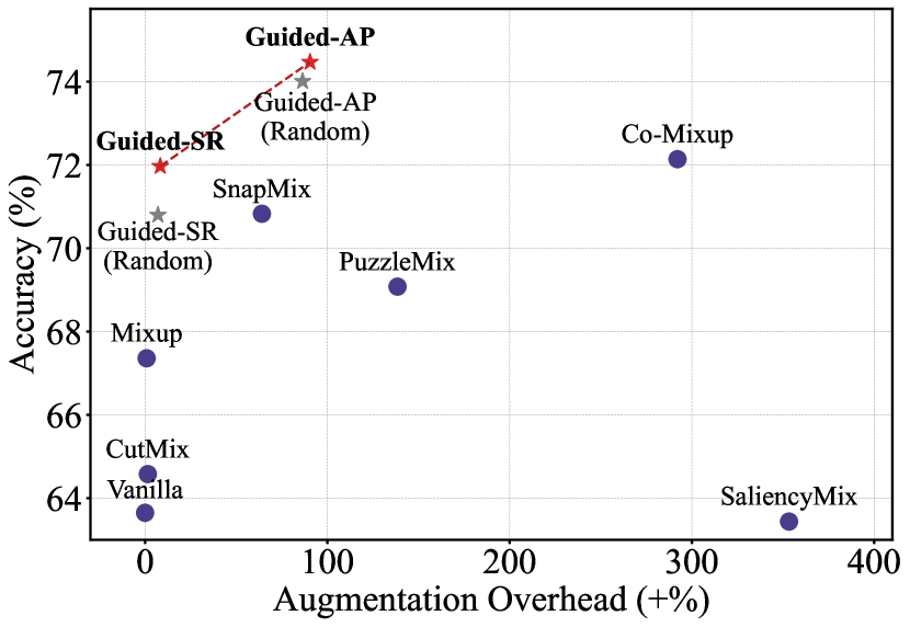
Figure 3: Augmentation overhead (+%) - accuracy (%) plot on CUB dataset with batch size 16. The closer to the upper left corner, the better the augmentation strategy is.

Method	Batch size	16	32	64
		Augmentation overhead (+%)
Mixup		0.9	0.6	0.4
CutMix		1.5	1.0	0.6
SaliencyMix		353.3	701.8	923.3
Guided-SR (Random)		6.4	4.2	2.7
Guided-SR (Greedy)		7.7	7.1	7.0
SnapMix		67.4	64.9	60.2
PuzzleMix		138.5	139.9	134.1
Co-Mixup		292.1	490.2	716.6
Guided-AP (Random)		87.8	81.9	70.1
Guided-AP (Greedy)		89.2	83.0	77.5

Table 2: Augmentation overhead ($\downarrow$, +%) of mixup methods with three different mini-batch sizes on CUB dataset.

5.3 Augmentation Overhead

In this section, we compare the computational efficiency of mixup strategies in addition to their generalization performance. To evaluate the computational efficiency, we utilize the augmentation overhead, which is the ratio of training time increased by including the augmentation as follows:

$$Augmentation\text{ }overhead=\frac{\textit{T}_{aug}-\textit{T}_{vanilla}}{\textit{T}_{vanilla}}\times 100(\%),$$

where T is the total training time, and $\textit{T}_{vanilla}$ is the training time without augmentation. In this evaluation, we compare the augmentation overhead without multi-processing during the augmentation process for a fair comparison.

Method	ResNet-18				ResNet-50				DenseNet-121
	CUB	Cars	Aircraft	Caltech	CUB	Cars	Aircraft	Caltech	CUB	Cars	Aircraft	Caltech
Vanilla	63.65	81.85	77.28	88.42	65.50	85.52	80.29	87.50	69.35	85.45	79.96	89.29
Mixup	67.36	85.14	79.39	90.15	71.33	88.14	82.38	91.01	74.23	89.06	81.73	91.47
CutMix	63.64	86.06	79.90	89.52	72.58	89.22	82.45	91.24	74.30	88.84	81.43	91.36
SaliencyMix	63.48	86.32	80.05	89.63	66.66	89.04	83.14	91.30	68.75	88.91	80.86	90.78
Guided-SR	71.95	86.50	80.94	90.66	74.08	89.23	83.51	91.36	76.51	89.40	83.22	91.82
SnapMix	70.83	87.45	80.64	89.75	75.53	90.10	82.96	90.78	75.76	90.27	83.29	91.36
PuzzleMix	69.08	87.27	79.18	90.44	74.85	89.68	82.66	90.53	77.27	90.10	82.63	91.47
Co-Mixup	72.14	87.59	80.23	90.03	72.83	89.53	83.57	90.38	77.05	90.23	83.35	90.44
Guided-AP	74.47	87.71	81.58	91.32	77.08	90.27	84.32	91.49	77.52	90.47	84.09	91.94

Table 3: Top-1 accuracy rate (%, $\uparrow$) on FGVC datasets using ResNet-18, ResNet-50, and DenseNet-121.

Figure 3 clearly shows the efficiency of our methods and confirms that both Guided-SR and Guided-AP are good trade-off solutions between generalization performance and augmentation overhead. Both methods enhance the accuracy rate up to 2% in each group, and Guided-SR is better than some methods with much bigger overhead. Also, we compare the augmentation overhead with three mini-batch sizes (16, 32, and 64) in Table 2. Another thing to note is that the overhead of Co-Mixup is about four times higher than that of Guided-AP, which utilizes the same saliency detection method, even with a small batch size of 16.

5.4 Generalization Performance on Fine-Grained Vision Classification (FGVC) Datasets

Classifying Fine-Grained Vision Classification (FGVC) datasets is a challenging task since the model needs to discriminate fine differences in the object. To check whether our method preserves the subtle object parts well, we compare GuidedMixup with the mixup baselines on four standard FGVC datasets using ResNet (He et al. 2016a) and DenseNet (Huang et al. 2017) architectures. Since previous mixup methods do not provide official reports on FGVC datasets, we reproduce their results based on the released codes. As shown in Table 3, our proposed methods improve the generalization performance with a large margin in each group. Especially, Guided-AP achieves state-of-the-art performance on all datasets.

Comparing the results of Guided-SR and Guided-AP in Table 1 and Table 3, Guided-AP consistently outperforms Guided-SR. This reconfirms that saliency detection in Guided-AP provides more precise saliency information than the spectral residual approach because it delivers information on what parts the model really cares about.

Method	Top-1 Err (%)	Corruption Err (%)
Vanilla	21.14	49.08
AugMix	20.45	32.22
Guided-SR	16.54	42.89
Guided-SR (Aug)	15.96	29.54
PuzzleMix	15.95	42.46
PuzzleMix (Aug)	16.60	29.91
Guided-AP	16.37	41.11
Guided-AP (Aug)	15.98	29.07

Table 4: Top-1 / mean Corruption Error rates (%, $\downarrow$) using WideResNet28-10 on CIFAR-100 and CIFAR-100-C. All the results are from PuzzleMix (Kim, Choo, and Song 2020).

Method	Clean		Corruption Type
	Top-1	Top5	Gaussian	Random
	Err (%)	Err (%)	Noise	Replacement
Vanilla	24.03	7.34	29.12	41.73
Input	22.97	6.48	26.29	39.41
CutMix	22.92	6.55	27.11	46.20
AugMix$\dagger$	23.25	6.70	-	-
Guided-SR	22.80	6.34	26.52	38.84
PuzzleMix	22.49	6.24	26.11	39.23
Co-Mixup	22.37	6.16	25.89	38.77
Guided-AP	22.47	6.14	24.66	38.72

Table 5: Top-1 and Top-5 error rates (%, $\downarrow$) on clean ImageNet dataset and Top-1 error rate (%) on corrupted ImageNet validation set (Kim et al. 2020) using ResNet-50. All the results are from PuzzleMix (Kim, Choo, and Song 2020), and Co-Mixup (Kim et al. 2020). The results of AugMix$\dagger$ on the corrupted dataset are not reported in the original paper.

5.5 Robustness on Corrupted Dataset and Scarce Dataset

Data Corruption Machine learning techniques assume that the training data distribution is similar to the test data distribution. Therefore, small corruption on the test data might cause mis-inference (LEE et al. 2020). In response to this issue, AugMix (Hendrycks et al. 2020) is one of the augmentation methods which cope well with corrupted images while improving generalization performance. In this section, we evaluate the robustness of our methods on corrupted datasets. Motivated by Kim, Choo, and Song (2020), we also tested GuidedMixup in combination with AugMix, which is an augmentation method that copes with corrupted images well. We simply use AugMix images as input for our methods, denoted as Guided-SR (Aug) and Guided-AP (Aug). CIFAR-100-C consists of 19 different corruptions (including blur, noise, weather, and digital corruption types), and we measure the average test error. In Table 4, we find that PuzzleMix with AugMix sacrifices the generalization performance to improve robustness. However, Guided-SR and Guided-AP combined with AugMix improve both generalization performance and robustness.

Next, we train ResNet-50 on ImageNet dataset for 100 epochs following the protocol of Kim et al. (2020) for evaluating both generalization and robustness. As shown in the ‘clean’ column of Table 5, Guided-AP is the second best, next to Co-Mixup, which has a significantly larger augmentation overhead as shown in Table 5.3. Considering this big difference in augmentation overhead, we believe Guided-AP provides a meaningful trade-off point even on ImageNet.

Also, there is the corrupted ImageNet validation set from Kim et al. (2020), which consists of the following two types of corrupted images; images partially random-replaced by other images and images distorted by random Gaussian noise. We evaluate the test errors on each corrupted dataset using ResNet-50 trained with each mixup strategy. As shown in Table 5, Guided-AP outperforms other mixup baselines for each corrupted dataset.

Data Scarcity Deep neural networks have suffered from data scarcity, which often causes overfitting. Because the primary purpose of augmentation is to regularize the model by effectively increasing the number of data, we evaluate the generalization performance under insufficient dataset conditions. We compare the accuracy of WideResNet28-10 (Zagoruyko and Komodakis 2016) trained with mixup strategies using only 10%, 20%, and 50% of the original CIFAR-100 dataset. In Table 6, both Guided-SR and Guided-AP show superior effectiveness when training data is more scarce. Moreover, we evaluate all the mixup baselines on Oxford 102 Flower dataset (Nilsback and Zisserman 2008), which has only 10 training images per class. Table 7 shows that our GuidedMixup consistently outperforms other mixup methods in situations where data is limited.

Method	The number of data per class
	50 (10%)	100 (20%)	250 (50%)
Vanilla	40.10 (0.70)	55.56 (0.21)	70.16 (0.17)
Input	49.44 (0.65)	61.74 (1.67)	74.31 (0.26)
Manifold	47.94 (0.70)	62.25 (0.43)	75.00 (0.16)
CutMix	42.81 (1.40)	60.14 (0.81)	74.94 (0.70)
Guided-SR	50.60 (0.48)	63.99 (0.49)	75.57 (0.10)
PuzzleMix	50.13 (0.84)	63.99 (0.16)	76.31 (0.27)
Co-Mixup	50.50 (0.98)	64.47 (0.63)	75.43 (0.12)
Guided-AP	54.25 (0.49)	66.22 (0.50)	76.70 (0.10)

Table 6: Top-1 accuracy rates (%, $\uparrow$) on CIFAR-100 with a reduced number of data per class using WideResNet28-10. The values in parentheses are the standard deviation of Top-1 accuracy rates. We experiment with three different seeds.

Method	Validation Acc (%)	Test Set Acc (%)
Vanilla	64.48 (1.60)	59.14 (1.15)
Mixup	70.55 (0.91)	66.81 (0.43)
CutMix	62.68 (2.20)	58.51 (0.42)
SaliencyMix	63.23 (1.19)	57.45 (1.00)
Guided-SR	72.84 (0.52)	69.31 (0.23)
SnapMix	65.71 (1.56)	59.79 (0.64)
PuzzleMix	71.56 (0.79)	66.71 (0.10)
Co-Mixup	68.17 (0.54)	63.20 (0.36)
Guided-AP	74.74 (0.40)	70.44 (0.69)

Table 7: Top-1 accuracy rates (%, $\uparrow$) on Flower dataset using ResNet-18. The values in parentheses are the standard deviation of Top-1 accuracy rates. We experiment with three different seeds.

5.6 Impact of Pairing Algorithm

GuidedMixup utilizes the proposed pairing algorithm in all the experiments to find good pairs among input images by utilizing a saliency map without handling a mixup mask. Therefore, This algorithm can also be applied to other mixup-based augmentation strategies. To verify the effectiveness of our pairing algorithm, we compare the performance of mixup baselines to whether the proposed pairing algorithm exists or not (in Table 8). The results indicate that our pairing algorithm is effective not only for our GuidedMixup, but also for most other mixup-based methods.

Method	Top-1 Accuracy (%)
	TinyImageNet	CUB	Aircraft
CutMix	57.81(+1.14)	64.41(+0.77)	80.09(+0.19)
SaliencyMix	58.19(+1.65)	63.88(+0.40)	80.37(+0.31)
Guided-SR	59.44(+0.51)	71.95(+1.15)	80.94(+0.44)
PuzzleMix	63.82(+0.34)	70.47(+1.49)	79.89(+0.71)
Guided-AP	64.63(+0.26)	74.47(+0.78)	81.58(+0.19)

Table 8: Top-1 accuracy rate (%, $\uparrow$) of the mixup methods with the proposed pairing algorithm on CUB and Aircraft datasets using ResNet-18 and on Tiny-ImageNet using PreActResNet-18. The values in parentheses are the improved accuracy by using our pairing algorithm.

6 Conclusion

We presented GuidedMixup, which generates a mixup image with objects from input images well preserved by efficiently determining mixup pairs and masks using the saliency information. Given mini-batch images, GuidedMixup selects pairs with minimally overlapping salient regions by an efficient and effective pairing algorithm. When mixing the chosen images, GuidedMixup adjusts the pixel-wise mixing ratio to maintain the salient regions of each image. Compared to previous mixup-based augmentation methods, GuidedMixup achieves the state-of-the-art generalization performance on CIFAR-100, Tiny-ImageNet, and all Fine-Grained Visual Classification datasets we tested, with much less computational overhead than previous optimization-based methods. In the data scarcity test, GuidedMixup performed better when the available training data gets smaller, reinforcing the merit of our method when data augmentation is more needed. Furthermore, our pairing algorithm can be independently used with other mixup strategies, leading to noticeable accuracy improvement. This also supports that maintaining salient regions is important in augmentation methods.

References

- Achanta et al. (2009) Achanta, R.; Hemami, S.; Estrada, F.; and Susstrunk, S. 2009. Frequency-tuned salient region detection. In 2009 IEEE conference on computer vision and pattern recognition, 1597–1604. IEEE.
- Bishop (1995) Bishop, C. M. 1995. Training with noise is equivalent to Tikhonov regularization. Neural computation, 7(1): 108–116.
- Bishop and Nasrabadi (2006) Bishop, C. M.; and Nasrabadi, N. M. 2006. Pattern recognition and machine learning, volume 4. Springer.
- Chrabaszcz, Loshchilov, and Hutter (2017) Chrabaszcz, P.; Loshchilov, I.; and Hutter, F. 2017. A downsampled variant of imagenet as an alternative to the cifar datasets. arXiv preprint arXiv:1707.08819.
- Deng et al. (2009) Deng, J.; Dong, W.; Socher, R.; Li, L.-J.; Li, K.; and Fei-Fei, L. 2009. Imagenet: A large-scale hierarchical image database. In 2009 IEEE conference on computer vision and pattern recognition, 248–255. Ieee.
- DeVries and Taylor (2017) DeVries, T.; and Taylor, G. W. 2017. Improved Regularization of Convolutional Neural Networks with Cutout. arXiv preprint arXiv:1708.04552.
- Edmonds (1965) Edmonds, J. 1965. Maximum matching and a polyhedron with 0,1-vertices. Journal of Research of the National Bureau of Standards Section B Mathematics and Mathematical Physics, 125.
- Fei-Fei, Fergus, and Perona (2006) Fei-Fei, L.; Fergus, R.; and Perona, P. 2006. One-shot learning of object categories. IEEE transactions on pattern analysis and machine intelligence, 28(4): 594–611.
- He et al. (2016a) He, K.; Zhang, X.; Ren, S.; and Sun, J. 2016a. Deep residual learning for image recognition. In Proceedings of the IEEE conference on computer vision and pattern recognition, 770–778.
- He et al. (2016b) He, K.; Zhang, X.; Ren, S.; and Sun, J. 2016b. Identity mappings in deep residual networks. In European conference on computer vision, 630–645. Springer.
- Hendrycks et al. (2020) Hendrycks, D.; Mu, N.; Cubuk, E. D.; Zoph, B.; Gilmer, J.; and Lakshminarayanan, B. 2020. AugMix: A Simple Data Processing Method to Improve Robustness and Uncertainty. Proceedings of the International Conference on Learning Representations (ICLR).
- Hou and Zhang (2007) Hou, X.; and Zhang, L. 2007. Saliency detection: A spectral residual approach. In 2007 IEEE Conference on computer vision and pattern recognition, 1–8. Ieee.
- Huang et al. (2017) Huang, G.; Liu, Z.; Van Der Maaten, L.; and Weinberger, K. Q. 2017. Densely Connected Convolutional Networks. In 2017 IEEE Conference on Computer Vision and Pattern Recognition (CVPR), 2261–2269. IEEE.
- Huang et al. (2016) Huang, G.; Sun, Y.; Liu, Z.; Sedra, D.; and Weinberger, K. Q. 2016. Deep networks with stochastic depth. In European conference on computer vision, 646–661. Springer.
- Huang, Wang, and Tao (2021) Huang, S.; Wang, X.; and Tao, D. 2021. SnapMix: Semantically Proportional Mixing for Augmenting Fine-grained Data. In Proceedings of the AAAI Conference on Artificial Intelligence.
- Itti, Koch, and Niebur (1998) Itti, L.; Koch, C.; and Niebur, E. 1998. A model of saliency-based visual attention for rapid scene analysis. IEEE Transactions on Pattern Analysis and Machine Intelligence, 20(11): 1254–1259.
- Kim et al. (2020) Kim, J.; Choo, W.; Jeong, H.; and Song, H. O. 2020. Co-Mixup: Saliency Guided Joint Mixup with Supermodular Diversity. In International Conference on Learning Representations.
- Kim, Choo, and Song (2020) Kim, J.-H.; Choo, W.; and Song, H. O. 2020. Puzzle mix: Exploiting saliency and local statistics for optimal mixup. In International Conference on Machine Learning, 5275–5285. PMLR.
- Krause et al. (2013) Krause, J.; Stark, M.; Deng, J.; and Fei-Fei, L. 2013. 3D Object Representations for Fine-Grained Categorization. In 4th International IEEE Workshop on 3D Representation and Recognition (3dRR-13). Sydney, Australia.
- Krizhevsky (2009) Krizhevsky, A. 2009. Learning Multiple Layers of Features from Tiny Images. Master’s thesis, University of Tront.
- Krizhevsky, Sutskever, and Hinton (2012) Krizhevsky, A.; Sutskever, I.; and Hinton, G. E. 2012. Imagenet classification with deep convolutional neural networks. Advances in neural information processing systems, 25.
- LEE et al. (2020) LEE, K.; Lee, K.; Shin, J.; and Lee, H. 2020. Network Randomization: A Simple Technique for Generalization in Deep Reinforcement Learning. In Eighth International Conference on Learning Representations, ICLR 2020. International Conference on Learning Representations.
- Lemley, Bazrafkan, and Corcoran (2017) Lemley, J.; Bazrafkan, S.; and Corcoran, P. 2017. Smart augmentation learning an optimal data augmentation strategy. Ieee Access, 5: 5858–5869.
- Maji et al. (2013) Maji, S.; Rahtu, E.; Kannala, J.; Blaschko, M.; and Vedaldi, A. 2013. Fine-grained visual classification of aircraft. arXiv preprint arXiv:1306.5151.
- Nilsback and Zisserman (2008) Nilsback, M.-E.; and Zisserman, A. 2008. Automated flower classification over a large number of classes. In 2008 Sixth Indian Conference on Computer Vision, Graphics & Image Processing, 722–729. IEEE.
- Simonyan, Vedaldi, and Zisserman (2013) Simonyan, K.; Vedaldi, A.; and Zisserman, A. 2013. Deep inside convolutional networks: Visualising image classification models and saliency maps. arXiv preprint arXiv:1312.6034.
- Srivastava et al. (2014) Srivastava, N.; Hinton, G.; Krizhevsky, A.; Sutskever, I.; and Salakhutdinov, R. 2014. Dropout: A Simple Way to Prevent Neural Networks from Overfitting. Journal of Machine Learning Research, 15(56): 1929–1958.
- Stanton et al. (2021) Stanton, S.; Izmailov, P.; Kirichenko, P.; Alemi, A. A.; and Wilson, A. G. 2021. Does Knowledge Distillation Really Work? arXiv preprint arXiv:2106.05945.
- Tutte (1954) Tutte, W. T. 1954. A Short Proof of the Factor Theorem for Finite Graphs. Canadian Journal of Mathematics, 6: 347 – 352.
- Uddin et al. (2020) Uddin, A. S.; Monira, M. S.; Shin, W.; Chung, T.; and Bae, S.-H. 2020. SaliencyMix: A Saliency Guided Data Augmentation Strategy for Better Regularization. In International Conference on Learning Representations.
- Verma et al. (2019) Verma, V.; Lamb, A.; Beckham, C.; Najafi, A.; Mitliagkas, I.; Lopez-Paz, D.; and Bengio, Y. 2019. Manifold mixup: Better representations by interpolating hidden states. In International Conference on Machine Learning, 6438–6447. PMLR.
- Wah et al. (2011) Wah, C.; Branson, S.; Welinder, P.; Perona, P.; and Belongie, S. 2011. The Caltech-UCSD Birds-200-2011 Dataset. Technical Report CNS-TR-2011-001, California Institute of Technology.
- Yun et al. (2019) Yun, S.; Han, D.; Oh, S. J.; Chun, S.; Choe, J.; and Yoo, Y. 2019. Cutmix: Regularization strategy to train strong classifiers with localizable features. In Proceedings of the IEEE/CVF International Conference on Computer Vision, 6023–6032.
- Zagoruyko and Komodakis (2016) Zagoruyko, S.; and Komodakis, N. 2016. Wide Residual Networks. In British Machine Vision Conference 2016. British Machine Vision Association.
- Zhang et al. (2018) Zhang, H.; Cisse, M.; Dauphin, Y. N.; and Lopez-Paz, D. 2018. mixup: Beyond Empirical Risk Minimization. In International Conference on Learning Representations.
- Zhao et al. (2015) Zhao, R.; Ouyang, W.; Li, H.; and Wang, X. 2015. Saliency detection by multi-context deep learning. In Proceedings of the IEEE conference on computer vision and pattern recognition, 1265–1274.
- Zhou et al. (2016) Zhou, B.; Khosla, A.; Lapedriza, A.; Oliva, A.; and Torralba, A. 2016. Learning deep features for discriminative localization. In Proceedings of the IEEE conference on computer vision and pattern recognition, 2921–2929.