rtables - A Framework For Creating Complex Structured Reporting Tables Via Multi-Level Faceted Computations

Abstract

Tables form a central component in both exploratory data analysis and formal reporting procedures across many industries. These tables are often complex in their conceptual structure and in the computations that generate their individual cell values. We introduce both a conceptual framework and a reference implementation for declaring, generating, rendering and modeling such tables. We place tables within the existing grammar of graphics paradigm for general statistical visualizations. Our open source rtables software implementation utilizes these connections to facilitate an intuitive way to declare complex table structure and construct those tables from data. In the course of this work, we relax several constraints present in the traditional grammar of graphics framing. Finally, rtables models instantiated tables as tree structures, which allows powerful, semantically meaningful and self-describing queries and manipulations of tables after creation. We showcase our framework in practice by creating complex, realistic example tables.

Keywords: visualization grammar graphics R clinical trials CSR

1 Introduction

Tabular summaries of information are a key method of both extracting and communicating information about a dataset or system. Complex tables are crucial to the analysis and reporting process in many contexts; this includes the pharmaceutical industry, where clinical trial reporting tables are an integral part of both the internal decision-making and external regulatory review processes.(U.S. FDA, 1996; Lancet, 2023) Other contexts with formal reporting table requirements include standard reporting by governmental statistical bureaus (U.S. BLS, 2023), and financial statements (U.S. SEC, 2020). Additionally, reporting tables are often included in news and academic articles in various forms.

‘Table’ is an overloaded term in computing; it can refer to a rectangular dataset intended primarily for consumption by computers (e.g., during analysis), or it can refer to a rectangular display of information or elements intended for human consumption. This conceptual distinction is crucial, despite some software’s willingness to allow users to create ‘tables’ which mix elements across these purposes (Broman and Woo, 2018).

Throughout this work we will use the term table exclusively as shorthand for reporting table: a table intended for human consumption which aggregates and/or summarizes some underlying data. We will use the term dataset to describe a rectangular set of data – whether raw or aggregate – intended for machine consumption.

Numerous software packages, both within and outside of the context of R, support the creation of tables. Microsoft Excel’s Pivot Tables (Microsoft Corporation, 2021) and SAS’s PROC TABULATE (SAS Institute, 2021) declare tabulations and cell value derivations in terms of variables and functions, following the precedent set by the US Bureau of Labor Statistics’ Table Producing Language (TPL) (Mendelssohn, 1974). Variables are used both to partition the data and to specify aspects of it to be summarized. Categorical variables define natural partitions of a dataset, and these tabulation systems use this to define subsets of data that correspond to rows, columns, and cells. They also allow nesting, i.e. consecutively subgrouping the data based on a sequence of variables.

Murdoch (2023)’s tables R package provides a robust port of SAS’s PROC TABULATE API where users generate nicely rendered tables by specifying the partitioning variables, analysis variables, and summary functions via formulas (Chambers and Hastie, 1992). R’s xtabs() function also provides an interface where users create tables by declaring the table structure via a formula, though nesting of partitions and customization of the computation performed on each subset is not supported. Numerous other packages implement cell value derivation and table rendering frameworks for specific types of tables (Sjoberg et al., 2021; Yoshida and Bartel, 2022).

The approach of declaring tabulation by categorical variables is also implemented by R’s aggregate() (R Core Team, 2023), which does not support nesting, as well as dplyr’s group_by() into summarise() workflow (Wickham et al., 2023) and data.table’s [, by=.] functionality (Dowle and Srinivasan, 2023) which do support nesting. These functions do not generate tables, however, but rather datasets of potential cell values.

Numerous R (R Core Team, 2023) packages provide fine-grained control and customization of the formatting of tables rendered into HTML (Ren and Russell, 2021; Iannone et al., 2023, Fillmore et al. (2023)), LaTeX and HTML (Dahl et al., 2019; Hugh-Jones, 2022) or numerous output formats (Daróczi and Tsegelskyi, 2022; Gohel and Skintzos, 2023; Yasumoto, 2023). These approaches do not provide mechanisms for computing the cell values to be displayed; rather they typically operate on a pre-existing dataset of cell values or model fit object and organize its elements into a table. Indications of complex structure, such as the appearance of multi-level grouping in column or row space are typically achieved by altering how a table should be displayed – often via post-processing – rather than being modeled in the table object.

Beyond R, McKinney et al. (2011)’s Pandas implements pivot tables, which support hierarchical grouping and complex aggregation in Python. Vink (2021)’s Polars, meanwhile, implements groupby mechanics similar to dplyr’s in both Python and Rust.

Clinical trial tables, in particular, can be complex both in two-dimensional structure and in the data manipulations and statistical calculations required to derive the individual cell values. These aspects of tabulation have a causal relationship not often exploited in existing tabulation frameworks: table structure implies the subsetting necessary to perform individual cell-value derivation, and vice versa.

Furthermore, the information encoded in this relationship remains useful beyond cell value derivation. Table rendering (including complex pagination), table post-processing, and quality-control checking can all make powerful use of this contextual information if retained.

We have developed a general tabulation framework - informed by the specific needs of clinical trial reporting - which retains and uses this intrinsic relationship between table structure, semantic meaning, and required computations. Our approach differs from and conceptually extends existing table-creation approaches in a number of ways. Like SAS, Excel, and the tables package, we allow complex tabulations to be declared symbolically. We generalize the declaration of these table structures beyond simple partitioning by categorical variables. We also fully separate the declaration of reusable, symbolic, data-instance agnostic table layouts from the process of performing the cell value derivations and constructing the table. Finally, the resulting tables are represented as a tree structure which reflects tabulations perform to create them, allowing for semantically meaningful subsetting and manipulation of the table’s elements.

We present here three aspects of our work on complex reporting tables. First, the rtables software itself and its ability to create complex tables are showcased in Section 2. Secondly, we place tables within Wilkinson (2005)’s overarching grammar of graphics and Wickham (2016)’s extension thereof in Section 3, and use this to motivate a conceptual framework for declaring and reasoning about data-summarizing table structures in Section 4. Finally in Section 5 we present an object model for instantiated tables which retain semantic information about the complex aggregations performed during their creation. We then conclude with a discussion of known limitations and future directions in Section 6.

2 Creating Structured Tables With rtables

Before discussing the details of rtables’ conceptual framework and design, we first use it to create some illustrative tables and discuss a case study of production level tables creation for clinical trial analyses and reporting.

2.1 Example Tables With Code

Creating a table with rtables is a two-part process. First we declare the conceptual structure of the table by creating a layout. Secondly, we apply that layout to a dataset to construct a table. The details of layout construction are discussed in Section 4. For detailed discussions of any of the functions used in this section, we refer readers to the rtables package documentation.

The rtables API, is fully general with no assumptions based on any particular data standards built in. In these examples, we will use synthetic data generated to the CDISC ADaM standards (CDISC ADaM Group, 2021) for clinical trial data for our example tables. Furthermore, we will use the default ASCII text rendering, but rendering to other formats including PDF, HTML and RTF is supported.

Our first example table is an adverse events table which summarizes event occurrences at two hierarchical levels of specificity, seen in Figure 1.

lyt <- basic_table(show_colcounts = TRUE) |>

  split_cols_by("ARM") |>

  analyze("USUBJID", afun = s_events_patients) |>

  split_rows_by("AEBODSYS", child_labels = "visible",

                split_fun = trim_levels_in_group("AEDECOD")) |>

  summarize_row_groups("USUBJID", cfun = s_events_patients) |>

  analyze("AEDECOD", table_count_once_per_id,

          show_labels = "hidden", indent_mod = -1)

tbl <- build_table(lyt, adae, alt_counts_df = adsl, hsep = "-")

tbl

                                           ARM A          ARM B
                                          (N=146)        (N=154)
-------------------------------------------------------------------
Patients with at least one event        114 (78.08%)   150 (97.40%)
Total events                                2060           1058
GASTROINTESTINAL
  Patients with at least one event      114 (78.08%)   146 (94.81%)
  Total events                              1344           675
  ABDOMINAL DISCOMFORT                      106             84
  ABDOMINAL FULLNESS DUE TO GAS             107             98
  GINGIVAL BLEEDING                          92             73
  NAUSEA (INTERMITTENT)                     110            109
MUSCULOSKELETAL AND CONNECTIVE TISSUE
  Patients with at least one event      113 (77.40%)   132 (85.71%)
  Total events                              716            383
  BACK PAIN                                  73             47
  WEAKNESS                                  111            123

Figure 1: This adverse event table groups events by body system organ class (AEBODSYS) and coded term (AEDECOD) and counts the number of subjects that experience the particular event at least once. Marginal group summaries at all levels display both total number of events and unique number of subjects in the group.

Our next example code generates a table (Figure 2) which summarizes overlapping (non-mutually exclusive) groups of observations. Here, we create a minimal demographics table which displays basic summary statistics for two demographic variables (SEX and AGE) separately for the biomarker evaluable population (BEP) and all patients within each arm, and for all patients across the study overall.

ex_adsl2$BEP <- sample(c("BEP", "Non-BEP"), nrow(ex_adsl2), replace = TRUE)

combodf <-  tribble(

    ~valname, ~label, ~levelcombo,         ~exargs,

    "ALL",    "All",  c("BEP", "Non-BEP"), list())

combo_lev_fun <- add_combo_levels(combodf, keep_levels = c("BEP", "ALL"))

lyt2 <- basic_table(show_colcounts = TRUE) |>

  split_cols_by("ARMCD") |>

  split_cols_by("BEP", split_fun = combo_lev_fun) |>

  add_overall_col("Overall") |>

  analyze("SEX", afun = counts_wpcts) |>

  analyze("AGE", afun = two_val_summary)

build_table(lyt2, ex_adsl2, hsep = "-")

                  ARM A                     ARM B
            BEP          All          BEP          All         Overall
           (N=41)       (N=96)       (N=48)       (N=94)       (N=190)
------------------------------------------------------------------------
SEX
  F      27 (65.9%)   59 (61.5%)   28 (58.3%)   52 (55.3%)   111 (58.4%)
  M      14 (34.1%)   37 (38.5%)   20 (41.7%)   42 (44.7%)   79 (41.6%)
AGE
  Mean      31.9         33.1         36.6         36.2         34.6
  sd        5.2          6.0          9.0          8.3           7.4

Figure 2: A table comparing two overlapping groups (BEP vs all patients) seperately within each arm, and collectively against the full patient population for the study.

Our next code constructs a table where different columns represent tabulation of entirely different variables, seen in Figure 3. We use split_cols_by_multivar() to define that type of column structure, and analyze_colvars() to specify the analysis.

lyt3 <- basic_table() |>

    split_cols_by("ARMCD") |>

    split_cols_by_multivar(c("AGE", "BMRKR1")) |>

    split_rows_by("SEX") |>

    analyze_colvars(three_val_summary)

build_table(lyt3, ex_adsl2, hsep = "-")

                       ARM A                      ARM B
                  AGE         BMRKR1         AGE         BMRKR1
-----------------------------------------------------------------
F
  Mean           32.1          5.7          34.7          5.5
  sd              5.9          3.2           7.9          3.3
  Min - Max   23.0 - 47.0   0.5 - 15.1   23.0 - 58.0   0.6 - 13.9
M
  Mean           34.6          6.5          38.0          5.7
  sd              6.1          4.1           8.5          3.2
  Min - Max   23.0 - 48.0   0.4 - 17.7   23.0 - 62.0   1.8 - 14.2

Figure 3: A table which analyzes two different variables (age, biomarker-1 measurement) as columns, within larger column faceting (by trial arm) and row faceting (sex).

Our last code example here demonstrates comparisons against a structural reference group resulting in the table shown in Figure 4. In particular, this table analyzes a (boolean) drug response including the fitting of statistical models where "ARM A" is considered the reference.

lyt4 <- basic_table(show_colcounts = TRUE) |>

  split_cols_by("ARMCD", ref_group = "ARM A") |>

  analyze("rsp", s_proportion, show_labels = "hidden") |>

  analyze("is_rsp", s_unstrat_resp, show_labels = "visible",

          var_labels = "Response Analysis")

build_table(lyt4, ADRS_BESRSPI, hsep = "-")

                             ARM A            ARM B             ARM C
                            (N=134)          (N=134)           (N=132)
--------------------------------------------------------------------------
Responders               114.0 (85.1%)    90.0 (67.2%)      120.0 (90.9%)
Non-Responders           20.0 (14.9%)     44.0 (32.8%)       12.0 (9.1%)
Response Analysis
  Diff Resp Rates (%)                         -17.9              5.8
  95% CI (Wald)                           (-27.9, -7.9)     (-1.9, 13.6)
  p-value (Chi^2 Test)                       0.0006            0.1436
  Odds Ratio (95% CI)                    0.4 (0.2 - 0.7)   1.8 (0.8 - 3.8)

Figure 4: A table analyzing response rate across arms of our fictional study. We note the two separate analyze blocks which go into different levels of detail.

Having now seen the code to create various complex tables with rtables we take a step back to place tables within the larger context of statistical visualization. We will then present our framework for declaring complex tables and our object model for representing and interacting with them.

2.2 Case Study: TLG-Catalog

Our framework is used for production table generation at Roche. This can be seen in the open source TLG-Catalog (NEST SME Team, 2023) developed and maintained by subject matter experts within the NEST team. The TLG-Catalog is a collection of more than 220 production ready table templates for use in clinical trials analyses and reporting.

The statistical and business specific logic in TLG-Catalog tables is implemented in the open source tern package (Zhu et al., 2023). tern, in turn, wraps and utilizes rtables’ layouting and tabulation frameworks.

3 Tables As Faceted Data Visualizations

Wilkinson (2005, ch. 11) notes that tables are graphs (emph. his); he does not, however, elaborate on this or how tables fit meaningfully into his grammar. We do that now.

Consider a standard two-way frequency table of whether a car is automatic against its number of gears using the mtcars dataset included with R:

mtcars2 <- mtcars

mtcars2$am <- factor(mtcars2$am, labels = c("Man", "Auto"))

table(transmission = mtcars2$am, gears = mtcars2$gear)

            gears
transmission  3  4  5
        Man  15  4  0
        Auto  0  8  5

Figure 5: Frequency table of transmission type vs number of gears, built with R’s table().

Viewed in the Wilkinsonian paradigm, we can frame the above as a faceted data visualization. The facets are the rows and columns of the table, while the subplots each contain the corresponding count rendered as text, as illustrated by the code in Figure 6.

DATA: mtcars2
DATA: xpos = constant(.5)
DATA: ypos = constant(.5)
COORD: rect(dim(3,4), dim(1,2))
SCALE: linear(dim(1), min(0), max(1))
SCALE: linear(dim(2), min(0), max(1))
ELEMENT: point(position(xpos*ypos*am*gear), size(0),
               label = summary.count(gear*am))

Figure 6: Grammar of Graphics code declaring our two-way frequency table.

This defines a faceted coordinate system, with 2D frames representing constant variables (xpos and ypos) embedded within 2D facet frames representing am and gear. Points are then “drawn” – with size zero – at the values of the constant variables, the center of the embedded frames, and labeled with the observation count.

The above is equivalent to the following code using Wickham (2016)’s layered extension of Wilkinson’s grammar for R, which recapitulates our two-way frequency table as a graph in Figure 7.

mtcars2[, c("xpos", "ypos")] <- .5

ggplot(data = mtcars2,  mapping = aes(x = xpos, y = ypos)) +

    geom_text(stat = StatCount2) +

    table_theme +

    facet_grid(rows = vars(am), cols = vars(gear), switch = "y") +

    scale_x_discrete(position = "top", name = "Gears") +

    scale_y_discrete(position = "left", name = "Transmission")

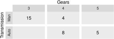
Figure 7: Our two-way frequency table of transmission type against number of gears, rendered using Wickham’s ggplot2 framework.

Indeed, each conceptual piece of a data-summarizing table maps to an analogous portion of a corresponding faceted data visualization. We illustrate this relationship directly in Figure 8 and Table LABEL:tab:map_to_grammar.

Our mapping onto Wilkinson’s grammar shows how tables fit within the existing paradigm while highlighting our generalizations. These generalizations include 1) relaxing the concept of faceting, 2) allowing for marginal summarizations at multiple levels in the row-hierarchy, 3) allowing different facet panes to display different analysis elements. We motivate and discuss these three extensions in the next section.

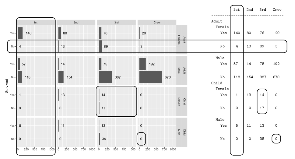
Figure 8: Analogous table and faceted barplot summarizing the Titanic death data included with R. Components of the table are highlighted both on the table and the barplot to emphasize their equivalence.

Table 1: Mapping Table Elements To Plot Components and Grammar Elements

() Table Component	Component in Faceted Barplot	In Grammar
()
Cell	Individual bar	ELEMENT / stat + geom
Row	Multiple bars across subplots (horizontal)	ELEMENT / stat + geom
Row group	Multiple subplots (horizontal)	COORD / facet_grid (Y dim)
Group Summary Row	Not Shown - Multiple marginal subplots	COORD / geom_xside*
Column or Col. Group	Multiple subplots (vertical)	COORD / facet_grid (X dim)
Vertical Cell Group	Subplot	ELEMENT / stat + geom
()

4 Pre-Data Layouts - Declaring Table Structure

Faceted plots are made up of (sub)plots which are themselves plotted within the coordinate system defined by the faceting (Wilkinson, 2005). Furthermore, we have shown that tables are faceted data visualizations. At its core, then, a table has two components:

1. A 2-dimensional faceting structure (COORD), and

2. a set of computations to be performed within each facet (ELEMENT).

With rtables, users build up a pre-data table layout which symbolically declares both aspects of their desired table and then apply it to a dataset to create the table.

4.1 Incrementally Declaring Facet Structure For Tables

In rtables, we declare facet structure by repeatedly splitting a pre-data table layout independently in both row and column dimensions. At each step, we are ‘splitting’ each existing facet in the relevant dimension further by nesting additional faceting within the current structure. This provides the intuitive, pipe-friendly workflow for declaring complex hierarchical faceting that we saw in Section 2.

In faceted visualizations, every facet corresponds to a specific subset of the overall data. Faceting, then, is the act of mapping an incoming parent dataset into the set of datasets corresponding to the facets the parent will be split into. In the grammar of graphics, this mapping is a partitioning of the dataset by a categorical variable. We generalize this concept by allowing faceting to be any mapping which goes maps an input dataset to a collection of one or more subsets of that dataset; in particular these subsets are not required to be exhaustive nor are they required to be mutually exclusive. We call this type of mapping a split function. rtables allows users to customize split functions at the level of individual faceting instructions. This allows users to declare table structures where different levels of faceting use different mappings, even within the same overall faceting dimension. We saw this in practice in column structure of the table rendered in Figure 3.

Non-mutually-exclusive types of faceting that are particularly useful for tables include those which add an “all” category alongside an otherwise normal partitioning of the dataset, those that compare a particular category to all observations - as we saw in Figure 2, and those that split data based on the cumulative quantiles of a continuous variable.

Most commonly, however, split functions will define facets by either partitioning the incoming data based on a categorical variable (split_rows_by(), split_cols_by()) or selecting different individual variables from the full incoming dataset (split_cols_by_multivar(), split_rows_by_multivar()). Partitioning based on categorical variables is equivalent to traditional faceting implemented in ggplot2 in both dimensions, and to SQL’s GROUP BY in the row dimension. (Wickham, 2016; ISO/IEC SC 32, 2016)

Splits in row-space always define structural groups of rows; individual rows are declared by summarizing row groups and analyzing data within them. We present these aspects of our framework below.

4.2 Declaring Cell Values - Summarizing and Analyzing

The cell contents of a table are declared orthogonally from its faceting structure, via interspersed use of the analyze and summarize row group verbs (analyze(), analyze_colvars(), summarize_row_groups()). Analyses map the data of a facet pane to a collection of cells analogous to a single subplot, which we call a vertical cell group. Applied across all levels of column-faceting, then, each analyze instruction defines a group of one or more rows in the resulting table.

Group summaries are similar to analyses with the exception that they can be declared at any point in the hierarchy of the row faceting structure. They act as marginal analyses, summarizing the data at higher levels of aggregation and providing semantic context to any analysis and even other summary rows nested within their facet. We saw this in practice in the adverse events table in Section 2.

Analyses and group summaries are specified via analysis functions and summary functions, respectively. These functions accept data associated with a facet and return a vertical cell group. Specifying these functions gives users full control over cell value derivation for their table.

5 Table Structure

Tables are created by applying a layout to data; rtables models tables as a set of analysis rows hierarchically grouped into subtables which make up a TableTree. Thus our tables are row dominant unlike data.frames in R which are column dominant. A TableTree’s structure maps directly to the row-dimension faceting declared by the layout used to create it. Each faceting instruction maps to a subtable (the split itself) containing a set of children representing the facets defined by the split. These children then contain subtables representing either further nested splitting, or representing the set of rows generated by an analyze() directive. Figure 9 illustrates this relationship, which we detail throughout this section.

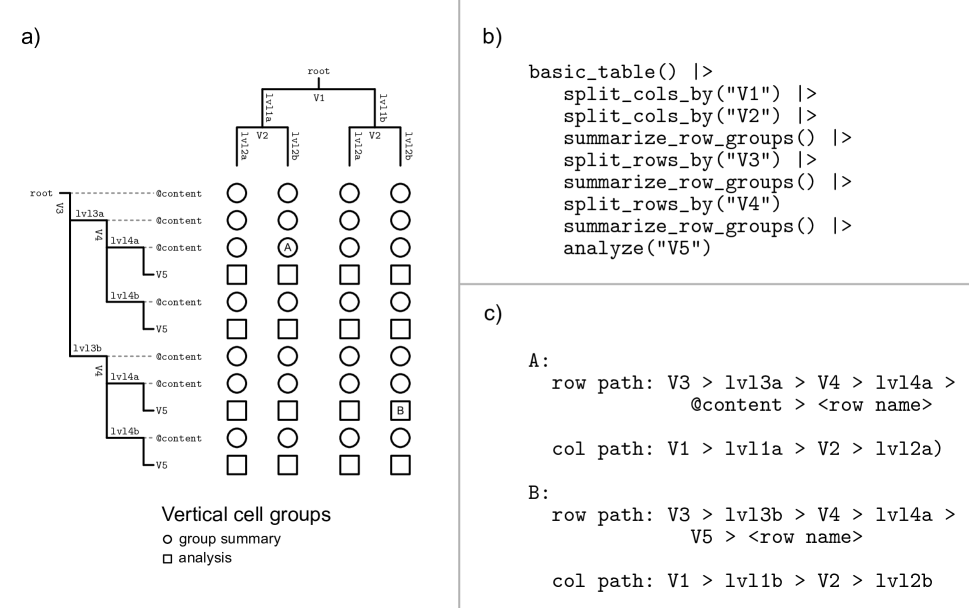
Figure 9: Relationship between layout, table and paths. a) the rectangular array of vertical cell groups (VCGs) annotated with the row and column tree structure; b) code which defines the layout for the table; c) example row- and column-paths for labelled cells within the table in (a). Circles in (a) represent VCGs containing marginal group summaries declared via summarize_row_groups() calls in (b), while squares represent VCGs declared in the analyze() call. The edge labels within the trees in (a) depict path components seen in (c).

5.1 Modeling Context And Group Summary Information

Representing tables as tree structures allows rtables to model optional group summary information which can be displayed when the table is rendered. These summaries provide visual context for the individual analysis rows within their facet. We model this contextual information in two forms: label rows, and content tables. Label rows provide context by associating a descriptive label to a row-space facet. Content tables extend the concept of label rows in two ways: they can contain multiple rows, and they contain non-empty cell values which provide context within their respective column to the full facet. We saw both of these types of contextual information in Section 2.

Content tables are created when executing the summarize_row_groups() layouting directive and are a flat collection of (typically) one or more content rows. These content rows are structurally identical to but semantically different from analysis rows. They act as an extension – and when present typically a replacement – of label rows by providing both labeling and a marginal summarization of the subtable (and implied group within the data).

5.2 Pathing

TableTrees’ tree structure allows us to define pathing for describing location within a table, similar to but much simpler than XPath (Clark and DeRose, 1999) defines for XML. We show examples of these paths in part (c) of Figure 9.

Paths provide a semantically meaningful way to describe location within the structure of a complex table. For example, the paths to the element labeled A in Figure 9 correspond to the elements which represent:

• rows which marginally analyze the data where the values of V3 and V4 are lvl3a and lvl4a, respectively; and

• columns within those rows corresponding to the data where the values of V1 and V2 are lvl1a and lvl2a, respectively.

These paths are guaranteed to be descriptive, predictable and deterministic . This allows analysts to use paths prescriptively, particularly when the data being summarized adhere to a formal specification. This is especially powerful, e.g., for selecting cell values to be included inline in reports such as those in clinical study reports (CSRs), for defining quality control (cross) checks for a class of tables, and for defining templates for automatically generated narrative reports.

Using these paths we can perform semantically meaningful subsetting of a table in both the row and column dimensions. Pathing also allows us to perform powerful structurally-aware manipulations of table content after creation. These notably include modifying or adding: raw cell values; formatting instructions for table elements; and referential footnotes.

Pathing also facilitates powerful manipulations of a table’s structure. These types of modifications include insertion of rows at structurally-valid points in the table, as well as sorting or pruning children based on - typically group summary - cell values within them. For details on these operations we refer our readers to the documentation for the insert_row_at_path(), sort_at_path() and prune_table() functions, respectively.

5.3 Analysis Results Datasets (ARDs)

The pharmaceutical industry is currently exploring the concept of Analysis Results Datasets (ARDs)(CDISC ARS Group, 2023) which represents cell content values as a dataset without the two dimensional table organization. Motivations for working with ARDs include broad accessibility and reusability of cell content values.

The concept of ARDs, however, does not address the primary difficulty in generating complex, multi-faceted tables: the cell value generation itself. rtables solves this difficulty as demonstrated throughout this paper. We provide the proof-of-concept as_ard() function which creates a semi-long form data.frame which combines the cell values from a table with metadata reflecting location in the faceting structure for that cell. As the ARD specifications evolves we update our function to meet them.

6 Discussion

We presented the rtables framework and showed how it can be used to create complex, data summarizing tables including those used for regulatory submission within the pharmaceutical industry. We then placed tables within the larger context of data visualizations by showing how they fit within Wilkinson’s grammar of graphics. Finally, we described an object model for representing and computing on complex tables.

In the next section, we will address some known limitations of both our conceptual framework and our implementation of it in rtables. Finally, we will briefly discuss possible future directions for our work.

6.1 Limitations

Arguably the largest limitation of the rtables approach is, simply put, that the resulting tables are not data.frames. While this is intentional, and powers the computations mentioned in Section 5.2 and others omitted for brevity (e.g. context preserving pagination), the fact remains that in some cases, users are likely to want to perform further analyses on a table’s cell values. Most analysis and visualization tooling in R assume data in a vector or data.frame format. Our as_ard() function derives a dataset which fully mitigates such concerns.

Another limitation of our framework is that neither layouts nor the resulting tables are transposable due to the fact that analyses are declared exclusively in row-structure space. While this does cause difficulty in creating certain column-dominant table structures in our framework, the split_cols_by_multivar() layout directive can force many of these tables into being. Furthermore, in the very few cases we have seen in practice where the desired gross-structure of a table was not achievable with rtables, an equivalently informative row-dominant table that was amenable to our framework has always existed.

Finally, rtables is complex, and likely to have a rather steep learning curve for novice users. We do not contest this assertion, but rather argue – we hope persuasively – that this complexity leads directly to the ease of performing very complex, powerful tabulations once the user is familiar with it.

6.2 Future Directions

Future directions of our work on rtables involve three components: extensions and advancements to the conceptual framework underpinning the software, improvements to the functionality of the software itself, and the reseeding of extensions and generalizations we made in the table context to the larger arena of visualization. We will briefly discuss possible future work of each type.

One avenue of future work is the incorporation of statistical plots into tables. While cell values can be anything, and thus – in the case of grid (R Core Team, 2023) or ggplot2 at least – can be graphics themselves, the rtables rendering machinery does not meaningfully support this. Similarly, support for rendering a table within or alongside a compound visualization is another piece of functionality we would like to add in the future.

We also plan to look into the creation of tables where the input data is not a single rectangular dataset. We expect that because all relational databases can be denormalized into single (very inefficient) rectangular datasets, the majority of things supported in rtables should translate fairly easily into multi-dataset input data, but the work to prove that – and to overcome the obstacles surely hiding in the details – remain to be done.

Another avenue of future work is making rtables-generated tables transposable. This could be done by fundamentally modifying our conceptual model or by implementing (pseudo-)transposition during rendering.

Additionally, rtables has been conceived as a way to create static tables. Determining where our framework fits within a space where static tables are still crucial but interactive tabulation is increasingly important could well define the next stage of rtables’ life-cycle.

Finally, we relaxed a number of restrictions inherent in the grammar of graphics as it was defined by Wilkinson and extended by Wickham. Chief amongst these were that:

1. Facets need not be a partition of incoming data, but rather a generalized grouping;

2. Marginal sub-‘plots’ can be defined at any point in the row faceting hierarchy; and

3. Elements defining subplots need not be the same across all parts of the facet grid.

While these advances were specifically necessary for tables, we feel they have value in the larger context of visualization generally. We hope to explore this in future work beyond rtables.

7 Availability

The rtables R package is available under the commercially permissive Apache 2.0 open source software license. The current production version can be installed from CRAN while development versions can be found – and issues filed – at http://github.com/insightsengineering/rtables. rtables is copyright F. Hoffman-La Roche, Ltd.

References

- Broman and Woo (2018) Broman, K. W. and Woo, K. H. (2018), “Data Organization in Spreadsheets,” The American Statistician, 72, 2–10, URL https://doi.org/10.1080/00031305.2017.1375989.
- CDISC ADaM Group (2021) CDISC ADaM Group (2021), ADaM Implementation Guide v1.3.
- CDISC ARS Group (2023) CDISC ARS Group (2023), “Project To Develop An ARD Standard,” https://www.cdisc.org/standards/foundational/analysis-results-standards.
- Chambers and Hastie (1992) Chambers, J. and Hastie, T. (1992), “Statistical Models. Chapter 2 of Statistical Models in S,” .
- Clark and DeRose (1999) Clark, J. and DeRose, S. (1999), “XML Path Language (XPath) Version 1.0, W3C Recommendation 16 November 1999,” .
- Dahl et al. (2019) Dahl, D. B., Scott, D., Roosen, C., Magnusson, A., and Swinton, J. (2019), xtable: Export Tables to LaTeX or HTML, URL https://CRAN.R-project.org/package=xtable. R package version 1.8-4.
- Daróczi and Tsegelskyi (2022) Daróczi, G. and Tsegelskyi, R. (2022), pander: An R ’Pandoc’ Writer, URL https://CRAN.R-project.org/package=pander. R package version 0.6.5.
- Dowle and Srinivasan (2023) Dowle, M. and Srinivasan, A. (2023), data.table: Extension of ‘data.frame‘, URL https://CRAN.R-project.org/package=data.table. R package version 1.14.8.
- Fillmore et al. (2023) Fillmore, C., Hughes, E., Krouse, B., Ahmad, K., and Haughton, S. (2023), tfrmt: Applies Display Metadata to Analysis Results Datasets, URL https://CRAN.R-project.org/package=tfrmt. R package version 0.0.3.
- Gohel and Skintzos (2023) Gohel, D. and Skintzos, P. (2023), flextable: Functions for Tabular Reporting, URL https://CRAN.R-project.org/package=flextable. R package version 0.9.2.
- Hugh-Jones (2022) Hugh-Jones, D. (2022), huxtable: Easily Create and Style Tables for LaTeX, HTML and Other Formats, URL https://CRAN.R-project.org/package=huxtable. R package version 5.5.2.
- Iannone et al. (2023) Iannone, R., Cheng, J., Schloerke, B., Hughes, E., Lauer, A., and Seo, J. (2023), gt: Easily Create Presentation-Ready Display Tables, URL https://CRAN.R-project.org/package=gt. R package version 0.9.0.
- ISO/IEC SC 32 (2016) ISO/IEC SC 32 (2016), “ISO/IEC 9075 - Database Lanagauges - SQL,” Standard, International Organization for Standardization, Geneva, CH.
- Lancet (2023) Lancet (2023), “Randomised Controlled Trials (RCT) guidelines,” URL https://www.thelancet.com/pb/assets/raw/Lancet/authors/RCTguidelines-1668613849943.pdf.
- Landis (2022) Landis, J. (2022), ggside: Side Grammar Graphics, URL https://CRAN.R-project.org/package=ggside. R package version 0.2.2.
- McKinney et al. (2011) McKinney, W. et al. (2011), “pandas: a foundational Python library for data analysis and statistics,” Python for high performance and scientific computing, 14, 1–9.
- Mendelssohn (1974) Mendelssohn, R. C. (1974), “The Bureau of Labor Statistic’s Table Producing Language (TPL),” in Proceedings of the 1974 Annual Conference - Volume 1, ACM ’74, New York, NY, USA: Association for Computing Machinery, URL https://doi.org/10.1145/800182.810390.
- Microsoft Corporation (2021) Microsoft Corporation (2021), “Microsoft Excel,” http://office.microsoft.com/excel.
- Murdoch (2023) Murdoch, D. (2023), tables: Formula-Driven Table Generation, URL https://CRAN.R-project.org/package=tables. R package version 0.9.17.
- NEST SME Team (2023) NEST SME Team (2023), “TLG Catalog,” https://insightsengineering.github.io/tlg-catalog/.
- R Core Team (2023) R Core Team (2023), R: A Language and Environment for Statistical Computing, R Foundation for Statistical Computing, Vienna, Austria, URL https://www.R-project.org/.
- Ren and Russell (2021) Ren, K. and Russell, K. (2021), formattable: Create ’Formattable’ Data Structures, URL https://CRAN.R-project.org/package=formattable. R package version 0.2.1.
- SAS Institute (2021) SAS Institute (2021), “SAS 9.4,” http://sas.com.
- Sjoberg et al. (2021) Sjoberg, D. D., Whiting, K., Curry, M., Lavery, J. A., and Larmarange, J. (2021), “Reproducible Summary Tables with the gtsummary Package,” The R Journal, 13, 570–580, URL https://doi.org/10.32614/RJ-2021-053.
- U.S. BLS (2023) U.S. BLS (2023), “Reports,” https://www.bls.gov/opub/reports/.
- U.S. FDA (1996) U.S. FDA (1996), “Structure and Content of Clinical Study Reports,” Standard guidance, Food and Drug Administration, United States of America, Washington, USA.
- U.S. SEC (2020) U.S. SEC (2020), “Financial Reporting Manual,” Standard, United States Securities Exchange Commission, Washington DC, USA.
- Vink (2021) Vink, R. (2021), “Polars - Lightning-fast DataFrame library for Rust and Python,” https://www.pola.rs/.
- Wickham (2016) Wickham, H. (2016), ggplot2: Elegant Graphics for Data Analysis, Springer-Verlag New York, URL https://ggplot2.tidyverse.org.
- Wickham et al. (2023) Wickham, H., François, R., Henry, L., Müller, K., and Vaughan, D. (2023), dplyr: A Grammar of Data Manipulation, URL https://CRAN.R-project.org/package=dplyr. R package version 1.1.2.
- Wilkinson (2005) Wilkinson, L. (2005), The Grammar of Graphics (Statistics and Computing), Berlin, Heidelberg: Springer-Verlag.
- Yasumoto (2023) Yasumoto, A. (2023), ftExtra: Extensions for ’Flextable’, URL https://CRAN.R-project.org/package=ftExtra. R package version 0.6.0.
- Yoshida and Bartel (2022) Yoshida, K. and Bartel, A. (2022), tableone: Create ’Table 1’ to Describe Baseline Characteristics with or without Propensity Score Weights, URL https://CRAN.R-project.org/package=tableone. R package version 0.13.2.
- Zhu et al. (2023) Zhu, J., Sabanés Bové, D., Stoilova, J., Wang, H., Collin, F., Waddell, A., Rucki, P., Liao, C., and Li, J. (2023), tern: Create Common TLGs Used in Clinical Trials, URL https://CRAN.R-project.org/package=tern. R package version 0.8.3.