The forward-backward-forward algorithm with extrapolation from the past and penalty scheme for solving monotone inclusion problems and applications

Abstract: In this paper, we propose an improved iterative method for solving the monotone inclusion problem in the form of $0\in Ax+Dx+N_{C}(x)$ in real Hilbert space, where $A$ is a maximally monotone operator, $D$ and $B$ are monotone and Lipschitz continuous, and $C$ is the nonempty set of zeros of the operator $B$. Our investigated method, called Tseng’s forward-backward-forward with extrapolation from the past and penalty scheme, extends the one proposed by Bot and Csetnek [Set-Valued Var. Anal. 22: 313–331, 2014]. We investigate the weak ergodic and strong convergence (when $A$ is strongly monotone) of the iterates produced by our proposed scheme. We show that the algorithmic scheme can also be applied to minimax problems. Furthermore, we discuss how to apply the method to the inclusion problem involving a finite sum of compositions of linear continuous operators by using the product space approach and employ it for convex minimization. Finally, we present a numerical experiment in TV-based image inpainting to validate the proposed theoretical theorem.

keywords: Tseng’s algorithm, iterative methods, optimization problems, monotone inclusion problems, minimax problems, convergence analysis, Fitzpatrick function.

MSC(2010): 47H05, 47N10, 65K05

1 Introdunction

In the last decade, penalty schemes have become a popular approach for studying constrained or hierarchical optimization problems in Hilbert spaces, particularly for solving complex problems (see [[Attouch2011Czarnecki, AttouchCzarnecki2011, BotCsetnek2014, 2014BotCsetnek, BotCsetnekNimana2018, Noun2013Peypouquet, BanertBot2015]]). In this work, we intend to study the general monotone inclusion problem in the following form:

$$0\in Ax+Dx+N_{C}(x),$$ (1)

where $A:\mathcal{H}\rightrightarrows\mathcal{H}$ is a maximally monotone operator, $D:\mathcal{H}\rightarrow\mathcal{H}$ a (single-valued) monotone and $\eta^{-1}$-Lipschitz continuous operator with $\eta>0$, and $N_{C}:\mathcal{H}\rightrightarrows\mathcal{H}$ is the normal cone of the closed convex set $C\subseteq\mathcal{H}$ which is the nonempty set of zeros of another operator $B:\mathcal{H}\rightarrow\mathcal{H}$, which is a (single-valued) $\mu^{-1}$-Lipschitz continuous operator with $\mu>0$.

The problem (1) is the generalized version of the monotone inclusion problem

$$0\in Ax+N_{C}(x),$$ (2)

where $C=\arg\min\Psi\neq\emptyset$, and $\Psi:\mathcal{H}\rightarrow\mathbb{R}$ is a convex differentiable function with a Lipschitz gradient satisfying $\min\Psi=0$, which introduces a penalization function with respect to the constraint $x\in C$. Implicit and explicit discretized methods to solve the problem in (2) were proposed in [[AttouchCzarnecki2011, Attouch2011Czarnecki]]. Several subsequent penalty type numerical algorithms in the literature are inspired by the continuous nonautonomous differential inclusion investigated in [[Attouch2010Czarnecki]].

In case $A$ is the convex subdifferential of a proper, convex, and lower semicontinuous function $\Phi:\mathcal{H}\rightarrow\bar{\mathbb{R}}$, then any solution of (2) solves the convex minimization problem

$$\min_{x\in\mathcal{H}}\{\Phi(x):x\in\arg\min\Psi\}.$$ (3)

Consequently, a solution to this convex minimization can be approximated by using the same iterative scheme as in [[AttouchCzarnecki2011, Attouch2011Czarnecki]]. Futhermore, there are other methods for solving such optimization problem which are studied by several authors in the literature (see, for instance, [[Noun2013Peypouquet, Peypouquet2012, BotCsetnekNimana2018, BanertBot2015]]).

Normally, for the iterative algorithms for solving both monotone inclusion problems (1) and (2) in penalty scheme, weak ergodic convergence is proved (and strong convergence under the strong monotonicity of $A$) (see [[AttouchCzarnecki2011, Attouch2011Czarnecki, BanertBot2015, 2014BotCsetnek, BotCsetnek2014]]). In order to achieve the (ergodic) convergent results, the following hypotheses need to be assumed.

• For solving the problem (2) in case $C=\arg\min\Psi\neq\emptyset$ with the algorithm proposed by Attouch et al. [[AttouchCzarnecki2011, Attouch2011Czarnecki]], the Fenchel conjugate function of $\Psi$ (namely, $\Psi^{*}$) needs to fulfill some key hypotheses in this context, as shown below:

  $(H)\begin{cases}(i)&A+N_{C}\;\mbox{is maximally monotone and}\;zer(A+N_{C})\neq\emptyset;\\ (ii)&\mbox{For every }p\in\operatorname{ran}(N_{C}),\sum_{n\in\mathbb{N}}\lambda_{n}\beta_{n}\left[\Psi^{*}\left(\frac{p}{\beta_{n}}\right)-\sigma_{C}\left(\frac{p}{\beta_{n}}\right)\right]<+\infty;\\ (iii)&(\lambda_{n})_{n\in\mathbb{N}}\in\ell^{2}\setminus\ell^{1},\end{cases}$

  where $(\lambda_{n})_{n\in\mathbb{N}}$ and $(\beta_{n})_{n\in\mathbb{N}}$ are sequences of positive real numbers. Note that the hypothesis $(ii)$ of $(H)$ is satisfied when $\sum_{n\in\mathbb{N}}\frac{\lambda_{n}}{\beta_{n}}<+\infty$ and $\Psi$ is bounded below by a multiple of the square of distances to $C$, as described in [[Attouch2011Czarnecki]]. One such case is when $C=zerL$, where $L:\mathcal{H}\rightarrow\mathcal{H}$ is a linear continuous operator with closed range and $\Psi:\mathcal{H}\rightarrow\mathbb{R}$ is defined as $\Psi(x)=\frac{1}{2}\|Lx\|^{2}$. Further situations in which condition $(ii)$ is fulfilled can be found in [[AttouchCzarnecki2011], Section 4.1].

• For solving the problem (1) with a forward-backward type or Tseng’s type (or forward-backward-forward) algorithm proposed by Bot et al. in [[BanertBot2015, BotCsetnek2014, 2014BotCsetnek]], the required hypotheses involve the Fitzpatrick function associated to the maximally monotone operator $B$ and reads as:

  $(H_{fitz})\begin{cases}(i)&A+N_{C}\;\mbox{is maximally monotone and}\;zer(A+D+N_{C})\neq\emptyset;\\ (ii)&\mbox{For every }p\in\operatorname{ran}(N_{C}),\sum_{n\in\mathbb{N}}\lambda_{n}\beta_{n}\left[\sup\limits_{u\in C}\varphi_{B}\left(u,\frac{p}{\beta_{n}}\right)-\sigma_{C}\left(\frac{p}{\beta_{n}}\right)\right]<+\infty;\\ (iii)&(\lambda_{n})_{n\in\mathbb{N}}\in\ell^{2}\setminus\ell^{1}.\end{cases}$

  where $(\lambda_{n})_{n\in\mathbb{N}}$ and $(\beta_{n})_{n\in\mathbb{N}}$ are sequences of positive real numbers. Note that when $B=\partial\Psi$ and $\Psi(x)=0$ for all $x\in C$, then by (4) one can see that condition $(ii)$ of $(H)$ implies the second condition of $(H_{fitz})$, see [[BotCsetnek2014, 2014BotCsetnek]].

Bot and Csetnek [[BotCsetnek2014]] relaxed the cocoercivity of $B$ and $D$ to monotonicity and Lipschitzian. In this setting, a forward-backward-forward penalty type algorithm based on a method proposed by Tseng [[Tseng2000]] is introduced. The convergence properties of this algorithm are studied under $(H_{fitz})$ and the condition $\lim\sup_{n\rightarrow+\infty}\left(\frac{\lambda_{n}\beta_{n}}{\mu}+\frac{\lambda_{n}}{\eta}\right)<1$.

In recent years, Tseng’s forward-backward-forward algorithm has been modified by many researchers in various versions depending on the setting of the operators (see [[Tongnoi2022, BöhmSedlmayerCsetnekBot2022, Malitsky2020Tam, Rakhlin2013Sridharan, RakhlinSridharan2013]], and references therein). One such modification is the Tseng’s forward-backward-forward algorithm with extrapolation from the past, which is developed by using Popov’s idea [[Popov1980]] for the extragradient method with the extrapolated technique. This algorithm can store and reuse the extrapolated term in the next step of the iterative scheme, illustrated as

$$\underbrace{\begin{cases}y_{n}=J_{\gamma A}(x_{n}-\gamma B(x_{n})),\\ x_{n+1}=y_{n}+\gamma(B(x_{n})-B(y_{n})),\end{cases}}_{\text{Tseng's algorithm}}\quad\mbox{and}\quad\underbrace{\begin{cases}y_{n}=J_{\gamma A}(x_{n}-\gamma B(y_{n-1})),\\ x_{n+1}=y_{n}+\gamma(B(y_{n-1})-B(y_{n})).\end{cases}}_{\text{Tseng's algorithm with extrapolation from the past}}$$

where $\gamma$ satisfies some suitable condition for each method and $J_{A}$ is the resolvent operator of $A$. According to this scheme, it has the potential to reduce computational costs and energy consumption in practical applications.

Motivated by these considerations, we investigate the Tseng’s forward-backward-forward algorithm with extrapolation from the past involving a penalty scheme under certain hypotheses for solving the inclusion problem in (1). We prove its weak ergodic convergence and further the strong convergence when the operator $A$ is a strongly monotone operator in Section 3. Furthermore, we can extend our results in Section 3 to solve minimax problems as elaborated in Section 4. In Section 5, our proposed algorithm can be extended to solving more intricate problems involving the finite sum of composition of linear continuous operator with maximally monotone operators by using the product space approach, and the convergence results for our modified iterative method are also provided.

To broaden the applicability of our scheme, we also provide the iterative scheme and its convergence result for the convex minimization problem expressed in Section 6. Finally, we demonstrate a numerical experiment in TV-based image inpainting to ensure theoretical convergence results in Section 7.

2 Preliminaries

In this paper, we introduce some notations used throughout. We denote the set of positive integers by $\mathbb{N}$ and a real Hilbert space with an inner product $\langle\cdot,\cdot\rangle$ and the associated norm $\|\cdot\|=\sqrt{\langle\cdot,\cdot\rangle}$ by $\mathcal{H}$. A sequence $(x_{n})_{n\in\mathbb{N}}$ is said to converge weakly to $x$, if for any $y\in\mathcal{H}$, $\langle x_{n},y\rangle\rightarrow\langle x,y\rangle$, and we use the symbols $\rightharpoonup$ and $\rightarrow$ to represent weak and strong convergence, respectively. For a linear continuous operator $L:\mathcal{H}\rightarrow\mathcal{G}$, where $\mathcal{G}$ is another real Hilbert space, we define the norm of $L$ as $\|L\|=\sup\{\|Lx\|:x\in\mathcal{H},\|x\|\leq 1\}$. We also use $L^{*}:\mathcal{G}\rightarrow\mathcal{H}$ to denote the adjoint operator of $L$, defined by $\langle L^{*}y,x\rangle=\langle y,Lx\rangle$ for all $(x,y)\in\mathcal{H}\times\mathcal{G}$.

For a function $f:\mathcal{H}\rightarrow\bar{\mathbb{R}}$ (where $\bar{\mathbb{R}}:=\mathbb{R}\cup\{\pm\infty\}$ is the extended real line), we denote its effective domain by $\operatorname{dom}f=\{x\in\mathcal{H}:f(x)<+\infty\}$ and say that $f$ is proper if $\operatorname{dom}f\neq\emptyset$ and $f(x)\neq-\infty$ for all $x\in\mathcal{H}$. Let $f^{*}:\mathcal{H}\rightarrow\bar{\mathbb{R}}$, where $f^{*}(u)=\sup_{x\in\mathcal{H}}\{\langle u,x\rangle-f(x)\}$ for all $u\in\mathcal{H}$, be the conjugate function of $f$. We denote by $\Gamma(\mathcal{H})$ the family of proper, convex, and lower semicontinuous extended real-valued functions defined on $\mathcal{H}$. The subdifferential of $f$ at $x\in\mathcal{H}$, with $f(x)\in\mathbb{R}$, is the set $\partial f(x):=\{v\in\mathcal{H}:f(y)\geq f(x)+\langle v,y-x\rangle\;\forall y\in\mathcal{H}\}$. We take, by convention, $\partial f(x):=\emptyset$ if $f(x)\in{\pm\infty}$.

The indicator function of a nonempty set $S\subseteq\mathcal{H}$, denoted by $\delta_{S}:\mathcal{H}\rightarrow\bar{\mathbb{R}}$, is defined as follows: $\delta_{S}(x)=0$ if $x\in S$ and $\delta_{S}(x)=+\infty$ otherwise. The subdifferential of the indicator function is called the normal cone of $S$, denoted by $N_{S}(x)$. For $x\in S$, $N_{S}(x)=\{u\in\mathcal{H}:\langle y-x,u\rangle\leq 0\;\forall y\in S\}$, and $N_{S}(x)=\emptyset$ if $x\notin S$. It is worth noting that for $x\in S$, $u\in N_{S}(x)$ if and only if $\sigma_{S}(u)=\langle x,u\rangle$, where $\sigma_{S}$ is the support function of $S$. The support function is defined as $\sigma_{S}(u)=\sup_{y\in S}\langle y,u\rangle$. A cone is a set that is closed under positive scaling, i.e., $\lambda x\in S$ for all $x\in S$ and $\lambda>0$. The normal cone, which is a tool used in optimization, is always a cone itself.

Let $A$ be a set-valued operator mapping from a Hilbert space $\mathcal{H}$ to itself. We define the graph of $A$ as $GrA=\{(x,u)\in\mathcal{H}\times\mathcal{H}:u\in Ax\}$, the domain of $A$ as $\operatorname{dom}A=\{x\in\mathcal{H}:Ax\neq\emptyset\}$, and the range of $A$ as $\operatorname{ran}A=\{u\in\mathcal{H}:\exists x\in\mathcal{H}\;\mbox{s.t.}\;u\in Ax\}$. The inverse operator of $A$, denoted by $A^{-1}:\mathcal{H}\rightrightarrows\mathcal{H}$, is defined as $(u,x)\in GrA^{-1}$ if and only if $(x,u)\in GrA$. We also define the set of zeros of $A$ as $zerA=\{x\in\mathcal{H}:0\in Ax\}$. The operator $A$ is said to be monotone if $\langle x-y,u-v\rangle\geq 0$ for all $(x,u),(y,v)\in GrA$. Moreover, a monotone operator $A$ is said to be maximally monotone if its graph on $\mathcal{H}\times\mathcal{H}$ has no proper monotone extension. If $A$ is maximally monotone, then $zerA$ is a closed and convex set, and a point $z\in\mathcal{H}$ belongs to $zerA$ if and only if $\langle u-z,w\rangle\geq 0$ for all $(u,w)\in GrA$. Conditions ensuring that $zerA$ is nonempty can be found in [[BC-Book], Section 23.4].

The set-valued operator $A$ is said to be $\gamma$-strongly monotone with $\gamma>0$ if and only if $\langle x-y,u-v\rangle\geq\gamma\|x-y\|^{2}$ for all $(x,u),(y,v)\in GrA$. If $A$ is maximally monotone and strongly monotone, then the set of zeros $zerA$ is a singleton and thus nonempty (refer to [[BC-Book], Corollary 23.37]). A single-valued operator $A:\mathcal{H}\rightarrow\mathcal{H}$ is considered to be $\gamma$-cocoercive if $\langle x-y,Ax-Ay\rangle\geq\gamma\|Ax-Ay\|^{2}$, and $\gamma$-Lipschitz continuous (or $\gamma$-Lipschitzian) if $\|Ax-Ay\|\leq\gamma\|x-y\|$ for all $(x,y)\in\mathcal{H}\times\mathcal{H}$.

In optimization, the proximal operator is a common tool used to develope algorithms for solving problems that involve a sum of a smooth function and a nonsmooth function. The proximal operator of a function $f$ at a point $x$ is defined as the unique minimizer of the function $y\mapsto f(y)+\frac{1}{2}\|y-x\|^{2}$, denoted by $\text{prox}_{f}(x):\mathcal{H}\rightarrow\mathcal{H}$. The resolvent of $A$, denoted by $J_{A}:\mathcal{H}\rightrightarrows\mathcal{H}$, is defined as $J_{A}=(Id+A)^{-1}$ where $Id:\mathcal{H}\rightarrow\mathcal{H}$, $Id(x)=x$ for all $x\in\mathcal{H}$, is the identity operator on $\mathcal{H}$. Moreover, if $A$ is maximally monotone, then $J_{A}:\mathcal{H}\rightarrow\mathcal{H}$ is single-valued and maximally monotone (see [[BC-Book], Corollary 23.10]). Notice that $J_{\partial f}=(Id+\partial f)^{-1}=\text{prox}_{f}$ (see also [[BC-Book], Proposition 16.34]).

Fitzpatrick introduced the notation we use in this paper in [[Fitzpatrick1988]], and it has proved to be a useful tool for investigating the maximality of monotone operators using convex analysis techniques (see [[Bauschke2006, BC-Book]]). For a monotone operator $A$, we define its associated Fitzpatrick function $\varphi_{A}:\mathcal{H}\times\mathcal{H}\rightarrow\bar{\mathbb{R}}$ as follows:

$$\varphi_{A}(x,u)=\sup_{(y,v)\in GrA}\{\langle x,v\rangle+\langle y,u\rangle-\langle y,v\rangle\}.$$

This function is convex and lower semicontinuous, and it will be an important tool for investigating convergence in this paper.

If $A$ is a maximally monotone operator, then its Fitzpatrick function is proper and satisfies $\varphi_{A}(x,u)\geq\langle x,u\rangle$ for all $(x,u)\in\mathcal{H}\times\mathcal{H}$, with equality if and only if $(x,u)\in GrA$. In particular, the subdifferential $\partial f$ of any convex function $f\in\Gamma(H)$ is a maximally monotone operator (cf. [[Rockafellar1970]]), and we have $(\partial f)^{-1}=\partial f^{*}$. Furthermore, we have the inequality (see [[Bauschke2006]])

$$\varphi_{\partial f}(x,u)\leq f(x)+f^{*}(u)\quad\forall(x,u)\in\mathcal{H}\times\mathcal{H},$$ (4)

where $f^{*}$ is the convex conjugate of $f$.

Before we enter on a detailed analysis of the convergence result, we introduce some definitions of sequences and useful lemmas that will be used several times in the paper. Let $(x_{n})_{n\in\mathbb{N}\cup\{0\}}$ be a sequence in $\mathcal{H}$ and $(\lambda_{k})_{k\in\mathbb{N}\cup\{0\}}$ a sequence of positive numbers such that $\sum_{k\in\mathbb{N}\cup\{0\}}\lambda_{k}=+\infty$. Let $(z_{n})_{n\in\mathbb{N}\cup\{0\}}$ be the sequence of weighted averages defined as shown in [[Attouch2011Czarnecki, 2014BotCsetnek, BotCsetnek2014]]:

$$z_{n}=\frac{1}{\tau_{n}}\sum_{k=0}^{n}\lambda_{k}x_{k},\quad\mbox{where}\;\tau_{n}=\sum_{k=0}^{n}\lambda_{k}\;\forall n\in\mathbb{N}.$$ (5)

The following lemma is the Opial-Passty Lemma, which serves as a key tool for achieving the convergence results in our analysis.

Lemma 1 (Opial-Passty).

Let $T$ be a nonempty subset of real Hilbert space $\mathcal{H}$ and assume that $\lim_{n\rightarrow\infty}\|x_{n}-x\|$ exists for every $x\in T$. If every weak cluster point of $(x_{n})_{n\in\mathbb{N}}$(respectively $(z_{n})_{n\in\mathbb{N}}$) belongs to $T$, then $(x_{n})_{n\in\mathbb{N}}$(respectively $(z_{n})_{n\in\mathbb{N}}$) converges weakly to an element in $T$ as $n\rightarrow\infty$.

Another key lemma underlying our work is presented below, which establishes the existence of convergence and the summability of sequences satisfying the conditions of the lemma. This lemma has been sourced from [[AttouchCzarnecki2011]].

Lemma 2.

Let $(a_{n})_{n\in\mathbb{N}},(b_{n})_{n\in\mathbb{N}}$ and $(\epsilon_{n})_{n\in\mathbb{N}}$ be real sequences. Assume that $(a_{n})_{n\in\mathbb{N}}$ is bounded from below, $(b_{n})_{n\in\mathbb{N}}$ is nonnegative sequences, $(\epsilon_{n})_{n\in\mathbb{N}}\in\ell^{1}$ such that

$$a_{n+1}\leq a_{n}-b_{n}+\epsilon_{n}\quad\forall n\in\mathbb{N}$$

Then $(a_{n})$ is convergent and $(b_{n})_{n\in\mathbb{N}}\in\ell^{1}$.

3 Forward-backward-forward with extrapolation and penalty schemes

In this section, we will begin by presenting a problem introduced in [[BotCsetnek2014, 2014BotCsetnek]], which can be formulated as follows:

Problem 1: Let $\mathcal{H}$ be a real Hilbert space, $A:\mathcal{H}\rightrightarrows\mathcal{H}$ a maximally monotone operator, $D:\mathcal{H}\rightarrow\mathcal{H}$ a monotone and $\eta^{-1}$-Lipschitz continuous operator with $\eta>0$, $B:\mathcal{H}\rightarrow\mathcal{H}$ a monotone and $\mu^{-1}$-Lipschitz continuous operator with $\mu>0$ and suppose that $C=zerB\neq\emptyset$. The monotone inclusion problem that we want to solve is

$$0\in Ax+Dx+N_{C}(x).$$ (6)

Some methods to solve Problem 1 have been already studied in [[BotCsetnek2014, 2014BotCsetnek]] by using Tseng’s algorithm and penalty scheme. The iterative scheme presented below for solving Problem 1 draws inspiration from Tseng’s forward-backward-forward algorithm with extrapolation from the past (see [[Tongnoi2022, BöhmSedlmayerCsetnekBot2022, Malitsky2020Tam]]).

where $(\lambda_{n})_{n\in\mathbb{N}\cup\{0\}}$ and $(\beta_{n})_{n\in\mathbb{N}\cup\{0\}}$ are sequences of positive real numbers.

Of course, in order to demonstrate the (ergodic) convergence results we need to assume the hypotheses $(H_{fitz})$ for every $n\in\mathbb{N}\cup\{0\}.$

Remark 3.

1. When the operator $B$ satisfies $Bx=0$ for all $x\in\mathcal{H}$ (which implies $N_{C}(x)={0}$ for every $x\in\mathcal{H}$), the algorithm outlined in Algorithm 1 reduces to the error-free scenario with the identity variable matrices of the forward-backward-forward with extrapolation method, as introduced in [[Tongnoi2022]].

2. Actually, we can choose $y_{-1}$ as any starting point in $\mathcal{H}$.

Prior to establishing the weak ergodic convergence result, we shall prove the following lemma, which serves as a valuable tool for our main outcome.

Lemma 4.

Let $(x_{n})_{n\in\mathbb{N}\cup\{0\}}$ and $(y_{n})_{{n\in\mathbb{N}\cup\{0,-1\}}}$ be the sequence generated by Algorithm 1 and let be $(u,w)\in Gr(A+D+N_{C})$ such that $w=v+p+D(u)$, where $v\in A(u)$ and $p\in N_{C}(u)$. Then the following inequlity holds for $n\in\mathbb{N}\cup\{0\}$:

$$\|x_{n+1}-u\|^{2}-\|x_{n}-u\|^{2}+\left(\frac{1}{2}-\left(\frac{\lambda_{n}\beta_{n}}{\mu}+\frac{\lambda_{n}}{\eta}\right)^{2}\right)\|y_{n-1}-y_{n}\|^{2}$$ (8)

$$\leq\left(\frac{\lambda_{n-1}\beta_{n-1}}{\mu}+\frac{\lambda_{n-1}}{\eta}\right)^{2}\|y_{n-2}-y_{n-1}\|^{2}+2\lambda_{n}\beta_{n}\left[\sup_{u\in C}\varphi_{B}(u,\frac{p}{\beta_{n}})-\sigma_{C}\left(\frac{p}{\beta_{n}}\right)\right]+2\lambda_{n}\langle u-y_{n},w\rangle.$$

Proof.

From Algorithm 1 and the definition of the resolvent, we can derive that $\forall n\in\mathbb{N}$

$$y_{n}=(Id+\lambda_{n}A)^{-1}[x_{n}-\lambda_{n}D(y_{n-1})-\lambda_{n}\beta_{n}B(y_{n-1})]\Leftrightarrow\frac{x_{n}-y_{n}}{\lambda_{n}}-D(y_{n-1})-\beta_{n}B(y_{n-1})\in A(y_{n}).$$ (9)

Thus, we have $\frac{x_{n}-y_{n}}{\lambda_{n}}-\beta_{n}B(y_{n-1})-D(y_{n-1})\in A(y_{n})$ for ever $n\in\mathbb{N}$. Since $v\in Au$, then we can guarantee by using the monotonicity of $A$ that

$$\langle y_{n}-u,\frac{x_{n}-y_{n}}{\lambda_{n}}-\beta_{n}B(y_{n-1})-D(y_{n-1})-v\rangle\geq 0\Leftrightarrow\langle y_{n}-u,x_{n}-y_{n}-\lambda_{n}\beta_{n}B(y_{n-1})-\lambda_{n}D(y_{n-1})-\lambda_{n}v\rangle\geq 0.$$ (10)

By using the definition of $x_{n+1}$, we obtain that $\forall n\in\mathbb{N}$,

$$\langle u-y_{n},x_{n}-y_{n}\rangle$$ (11)

$$\leq\langle u-y_{n},\lambda_{n}\beta_{n}B(y_{n-1})+\lambda_{n}D(y_{n-1})+\lambda_{n}v\rangle$$

$$\leq\langle u-y_{n},[\lambda_{n}\beta_{n}(B(y_{n-1})-B(y_{n}))+\lambda_{n}(D(y_{n-1})-D(y_{n}))+y_{n}]+\lambda_{n}\beta_{n}B(y_{n})+\lambda_{n}D(y_{n})+\lambda_{n}v-y_{n}\rangle$$

$$=\langle u-y_{n},x_{n+1}-y_{n}+\lambda_{n}\beta_{n}B(y_{n})+\lambda_{n}D(y_{n})+\lambda_{n}v\rangle$$

$$=\langle u-y_{n},x_{n+1}-y_{n}\rangle+\langle u-y_{n},\lambda_{n}\beta_{n}B(y_{n})\rangle+\langle u-y_{n},\lambda_{n}D(y_{n})\rangle+\langle u-y_{n},\lambda_{n}v\rangle.$$

For any $a_{1},a_{2},a_{3}\in\mathcal{H}$, we know that $\frac{1}{2}\|a_{1}-a_{2}\|^{2}-\frac{1}{2}\|a_{3}-a_{1}\|^{2}+\frac{1}{2}\|a_{3}-a_{2}\|^{2}=\langle a_{1}-a_{2},a_{3}-a_{2}\rangle$. Then, it follows from (11), we have that

$$\frac{1}{2}\|u-y_{n}\|^{2}-\frac{1}{2}\|x_{n}-u\|^{2}+\frac{1}{2}\|x_{n}-y_{n}\|^{2} \leq\frac{1}{2}\|u-y_{n}\|^{2}-\frac{1}{2}\|x_{n+1}-u\|^{2}+\frac{1}{2}\|x_{n+1}-y_{n}\|^{2}$$

$$\;+\langle u-y_{n},\lambda_{n}\beta_{n}B(y_{n})\rangle+\langle u-y_{n},\lambda_{n}D(y_{n})\rangle+\langle u-y_{n},\lambda_{n}v\rangle.$$

Because $v=w-p-Du$ and the fact that $D$ is monotone, we have that for every $n\in\mathbb{N}$

$$\|x_{n+1}-u\|^{2}-\|x_{n}-u\|^{2} \leq\|x_{n+1}-y_{n}\|^{2}-\|x_{n}-y_{n}\|^{2}+2\lambda_{n}\beta_{n}\langle u-y_{n},B(y_{n})\rangle+2\lambda_{n}\langle u-y_{n},D(y_{n})\rangle$$ (12)

$$\quad+2\lambda_{n}\langle u-y_{n},w-p-Du\rangle$$

$$=\|x_{n+1}-y_{n}\|^{2}-\|x_{n}-y_{n}\|^{2}+2\lambda_{n}\beta_{n}\langle u-y_{n},B(y_{n})\rangle$$

$$\quad+2\lambda_{n}\beta_{n}\langle u-y_{n},\frac{-p}{\beta_{n}}\rangle+2\lambda_{n}\langle u-y_{n},D(y_{n})-Du\rangle+2\lambda_{n}\langle u-y_{n},w\rangle$$

$$=\|x_{n+1}-y_{n}\|^{2}-\|x_{n}-y_{n}\|^{2}$$

$$\quad+2\lambda_{n}\beta_{n}\!\left(\!\!\langle u,B(y_{n})\rangle\!+\langle y_{n},\frac{p}{\beta_{n}}\rangle\!-\langle y_{n},B(y_{n})\rangle\!-\langle u,\frac{p}{\beta_{n}}\rangle\!\right)$$

$$\quad+2\lambda_{n}\underbrace{\langle u-y_{n},D(y_{n})-Du\rangle}_{\leq 0}+2\lambda_{n}\langle u-y_{n},w\rangle$$

$$\leq\|x_{n+1}-y_{n}\|^{2}-\|x_{n}-y_{n}\|^{2}$$

$$\quad+2\lambda_{n}\beta_{n}\left[\sup_{u\in C}\left\{\sup_{(s,Bs)\in GrB}\{\langle u,B(s)\rangle\!+\langle s,\frac{p}{\beta_{n}}\rangle\!-\langle s,B(s)\rangle\}\right\}-\sigma_{C}\left(\frac{p}{\beta_{n}}\right)\right]$$

$$\quad+2\lambda_{n}\langle u-y_{n},w\rangle$$

$$=\|x_{n+1}-y_{n}\|^{2}-\|x_{n}-y_{n}\|^{2}+2\lambda_{n}\beta_{n}\left[\sup_{u\in C}\varphi_{B}\left(u,\frac{p}{\beta_{n}}\right)-\sigma_{C}\left(\frac{p}{\beta_{n}}\right)\right]$$

$$\quad+2\lambda_{n}\langle u-y_{n},w\rangle.$$

By the Lipschitz continuity of $B$ and $D$, it yields

$$\|x_{n+1}-y_{n}\| =\|\lambda_{n}\beta_{n}(B(y_{n-1})-B(y_{n}))+\lambda_{n}(D(y_{n-1})-D(y_{n}))\|$$ (13)

$$\leq\lambda_{n}\beta_{n}\|B(y_{n-1})-B(y_{n})\|+\lambda_{n}\|D(y_{n-1})-D(y_{n})\|$$

$$=\left(\frac{\lambda_{n}\beta_{n}}{\mu}+\frac{\lambda_{n}}{\eta}\right)\|y_{n-1}-y_{n}\|.$$

It follows from (12) and above inequality that

$$\|x_{n+1}-u\|^{2}-\|x_{n}-u\|^{2} \leq\left(\frac{\lambda_{n}\beta_{n}}{\mu}+\frac{\lambda_{n}}{\eta}\right)^{2}\|y_{n-1}-y_{n}\|^{2}-\|x_{n}-y_{n}\|^{2}$$ (14)

$$\quad+2\lambda_{n}\beta_{n}\left[\sup_{u\in C}\varphi_{B}\left(u,\frac{p}{\beta_{n}}\right)-\sigma_{C}\left(\frac{p}{\beta_{n}}\right)\right]+2\lambda_{n}\langle u-y_{n},w\rangle.$$ (15)

By Parallelogram law, we know that $2\|x_{n}-y_{n}\|^{2}+2\|x_{n}-y_{n-1}\|^{2}=\|y_{n-1}-y_{n}\|^{2}+\|(x_{n}-y_{n})+(x_{n}-y_{n-1})\|^{2}$. Then we have

$$-\|x_{n}-y_{n}\|^{2}\leq\|x_{n}-y_{n-1}\|^{2}-\frac{1}{2}\|y_{n-1}-y_{n}\|^{2}.$$

So, we can derive from (14) that

$$\|x_{n+1}-u\|^{2}-\|x_{n}-u\|^{2} \leq\left(\frac{\lambda_{n}\beta_{n}}{\mu}+\frac{\lambda_{n}}{\eta}\right)^{2}\|y_{n-1}-y_{n}\|^{2}+\left[\|x_{n}-y_{n-1}\|^{2}-\frac{1}{2}\|y_{n-1}-y_{n}\|^{2}\right]$$

$$\quad+2\lambda_{n}\beta_{n}\left[\sup_{u\in C}\varphi_{B}\left(u,\frac{p}{\beta_{n}}\right)-\sigma_{C}\left(\frac{p}{\beta_{n}}\right)\right]+2\lambda_{n}\langle u-y_{n},w\rangle.$$

It follows from (13) that $\|x_{n}-y_{n-1}\|\leq\left(\frac{\lambda_{n-1}\beta_{n-1}}{\mu}+\frac{\lambda_{n-1}}{\eta}\right)\|y_{n-2}-y_{n-1}\|$. Thus,

$$\|x_{n+1}-u\|^{2}-\|x_{n}-u\|^{2} \leq\left(\frac{\lambda_{n}\beta_{n}}{\mu}+\frac{\lambda_{n}}{\eta}\right)^{2}\|y_{n-1}-y_{n}\|^{2}$$

$$\quad+\left[\left(\frac{\lambda_{n-1}\beta_{n-1}}{\mu}+\frac{\lambda_{n-1}}{\eta}\right)^{2}\|y_{n-2}-y_{n-1}\|^{2}-\frac{1}{2}\|y_{n-1}-y_{n}\|^{2}\right]$$

$$\quad+2\lambda_{n}\beta_{n}\left[\sup_{u\in C}\varphi_{B}\left(u,\frac{p}{\beta_{n}}\right)-\sigma_{C}\left(\frac{p}{\beta_{n}}\right)\right]+2\lambda_{n}\langle u-y_{n},w\rangle.$$

Therefore

$$\|x_{n+1}-u\|^{2}-\|x_{n}-u\|^{2}+\left(\frac{1}{2}-\left(\frac{\lambda_{n}\beta_{n}}{\mu}+\frac{\lambda_{n}}{\eta}\right)^{2}\right)\|y_{n-1}-y_{n}\|^{2}$$

$$\leq\left(\frac{\lambda_{n-1}\beta_{n-1}}{\mu}+\frac{\lambda_{n-1}}{\eta}\right)^{2}\|y_{n-2}-y_{n-1}\|^{2}+2\lambda_{n}\beta_{n}\left[\sup_{u\in C}\varphi_{B}\left(u,\frac{p}{\beta_{n}}\right)-\sigma_{C}\left(\frac{p}{\beta_{n}}\right)\right]+2\lambda_{n}\langle u-y_{n},w\rangle.$$

∎

Subsequently, we state the convergence of Algorithm 1 below.

Theorem 5.

Let $(x_{n})_{n\in\mathbb{N}\cup\{0\}}$ and $(y_{n})_{n\in\mathbb{N}\cup\{0,-1\}}$ be the sequences generated by Algorithm 1 and $(z_{n})_{n\in\mathbb{N}\cup\{0\}}$ be the sequence defined in (5). If ($H_{fitz}$) is fulfilled and $\limsup_{n\rightarrow+\infty}\left(\frac{\lambda_{n}\beta_{n}}{\mu}+\frac{\lambda_{n}}{\eta}\right)<\frac{1}{2}$, then $(z_{n})_{n\in\mathbb{N}\cup\{0\}}$ converges weakly to an element in $zer(A+D+N_{C})$ as $n\rightarrow+\infty$.

Proof.

The proof of the theorem divides into three parts as the following statements:

1. $\sum_{n\in\mathbb{N}\cup\{0\}}\|y_{n}-y_{n-1}\|^{2}<+\infty$ and the sequence $(\|x_{n}-u\|)_{n\in\mathbb{N}\cup\{0\}}$ is convergent for every $u\in zer(A+D+N_{C})$;

2. every weak cluster point of $(z^{\prime}_{n})_{n\in\mathbb{N}\cup\{0\}}$ lies in $zer(A+D+N_{C})$, where

   $$z^{\prime}_{n}=\frac{1}{\tau_{n}}\sum_{k=0}^{n}\lambda_{k}y_{k}\quad\mbox{and}\quad\tau_{n}=\sum_{k=0}^{n}\lambda_{k}\;\forall n\in\mathbb{N};$$

3. every weak cluster point of $(z_{n})_{n\in\mathbb{N}\cup\{0\}}$ lies in $zer(A+D+N_{C})$.

Every step of proof can be showed as follows.

(a) Let $u\in zer(A+D+N_{C})$. For $n\in\mathbb{N}$, we take $w=0$ in (8), so we have

$$\|x_{n+1}-u\|^{2}-\|x_{n}-u\|^{2}+\left(\frac{1}{2}-M_{n}^{2}\right)\|y_{n-1}-y_{n}\|^{2}$$ (16)

$$\leq M_{n-1}^{2}\|y_{n-2}-y_{n-1}\|^{2}+2\lambda_{n}\beta_{n}\left[\sup_{u\in C}\varphi_{B}\left(u,\frac{p}{\beta_{n}}\right)-\sigma_{C}\left(\frac{p}{\beta_{n}}\right)\right],$$

where $M_{n}=\frac{\lambda_{n}\beta_{n}}{\mu}+\frac{\lambda_{n}}{\eta}$. Rearranging the inequality, we have that

$$\|x_{n+1}-u\|^{2}+M_{n}^{2}\|y_{n-1}-y_{n}\|^{2}+\left(\frac{1}{2}-2M_{n}^{2}\right)\|y_{n-1}-y_{n}\|^{2}$$ (17)

$$\leq\|x_{n}-u\|^{2}+M_{n-1}^{2}\|y_{n-2}-y_{n-1}\|^{2}+2\lambda_{n}\beta_{n}\left[\sup_{u\in C}\varphi_{B}\left(u,\frac{p}{\beta_{n}}\right)-\sigma_{C}\left(\frac{p}{\beta_{n}}\right)\right].$$

By the hypothesis, we have that $\liminf_{n\rightarrow+\infty}\left(\frac{1}{2}-2M_{n}^{2}\right)>0$, it follows from Lemma 2 that the sequence $E_{n}:=\|x_{n}-u\|^{2}+M_{n-1}^{2}\|y_{n-2}-y_{n-1}\|^{2}$ converges and $\sum_{n\in\mathbb{N}}\|y_{n-1}-y_{n}\|^{2}<+\infty$. This means that $(\|y_{n-1}-y_{n}\|^{2})_{n\in\mathbb{N}\cup\{0\}}\rightarrow 0$ and so $(\|x_{n}-u\|)_{n\in\mathbb{N}\cup\{0\}}$ is a convergent sequence.

(b) Let $z$ be a weak cluster point of $(z^{\prime}_{n})_{n\in\mathbb{N}}$. Take $(u,w)\in Gr(A+D+N_{C})$ such that $w=v+p+Du$, where $v\in Au$ and $p\in N_{C}(u)$. Let $K\in\mathbb{N}$ with $\forall n_{0}\in\mathbb{N}$, $K\geq n_{0}+2$. Summing up for $n=n_{0}+1,\dots,K$ the inequalities in (8) (it is nothing else than (16) with the additional term $2\lambda_{n}\langle u-y_{n},w\rangle$) with $\limsup_{n\rightarrow+\infty}\left(\frac{\lambda_{n}\beta_{n}}{\mu}+\frac{\lambda_{n}}{\mu}\right)<\frac{1}{2}$, for $n\in\mathbb{N}$ and $M_{n}=\frac{\lambda_{n}\beta_{n}}{\mu}+\frac{\lambda_{n}}{\eta}$ we get that

$$\sum_{n=n_{0}+1}^{K}\|x_{n+1}-u\|^{2}-\sum_{n=n_{0}+1}^{K}\|x_{n}-u\|^{2} \leq\sum_{n=n_{0}+1}^{K}M_{n-1}^{2}\|y_{n-2}-y_{n-1}\|^{2}$$

$$\quad+2\sum_{n=n_{0}+1}^{K}\lambda_{n}\beta_{n}\left[\sup_{u\in C}\varphi_{B}\left(u,\frac{p}{\beta_{n}}\right)-\sigma_{C}\left(\frac{p}{\beta_{n}}\right)\right]$$

$$\quad+2\left\langle\sum_{n=0}^{K}\lambda_{n}u-\sum_{n=0}^{K}\lambda_{n}y_{n}-\sum_{n=0}^{n_{0}}\lambda_{n}u+\sum_{n=0}^{n_{0}}\lambda_{n}y_{n},w\right\rangle.$$

This leads to the following inequality.

$$\|x_{K+1}-u\|^{2}-\|x_{n_{0}+1}-u\|^{2} \leq\sum_{n=n_{0}+1}^{+\infty}M_{n-1}^{2}\|y_{n-2}-y_{n-1}\|^{2}+2\sum_{n=n_{0}+1}^{+\infty}\lambda_{n}\beta_{n}\left[\sup_{u\in C}\varphi_{B}\left(u,\frac{p}{\beta_{n}}\right)-\sigma_{C}\left(\frac{p}{\beta_{n}}\right)\right]$$

$$\quad+2\left\langle\sum_{n=0}^{K}\lambda_{n}u-\sum_{n=0}^{K}\lambda_{n}y_{n}-\sum_{n=0}^{n_{0}}\lambda_{n}u+\sum_{n=0}^{n_{0}}\lambda_{n}y_{n},w\right\rangle$$

$$=R+2\left\langle\sum_{n=0}^{K}\lambda_{n}u-\sum_{n=0}^{K}\lambda_{n}y_{n}-\sum_{n=0}^{n_{0}}\lambda_{n}u+\sum_{n=0}^{n_{0}}\lambda_{n}y_{n},w\right\rangle,$$

[]

$$\mbox{where}\;R=\sum_{n=n_{0}+1}^{+\infty}M_{n-1}^{2}\|y_{n-2}-y_{n-1}\|^{2}+2\sum_{n\geq n_{0}+1}^{+\infty}\lambda_{n}\beta_{n}\left[\displaystyle\sup_{u\in C}\varphi\left(u,\frac{p}{\beta_{n}}\right)-\sigma_{C}\left(\frac{p}{\beta_{n}}\right)\right]\in\mathbb{R}.$$

Discarding the nonnegative term $\|x_{K+1}-u\|^{2}$ and dividing $2\tau_{K}=2\sum_{n=1}^{K}\lambda_{n}$ we obtain

$$-\frac{\|x_{n_{0}+1}-u\|^{2}}{2\tau_{K}} \leq\frac{R+2\langle-\sum_{n=1}^{n_{0}}\lambda_{n}u+\sum_{n=1}^{n_{0}}\lambda_{n}y_{n},w\rangle}{2\tau_{K}}+\frac{2\langle\sum_{n=1}^{K}\lambda_{n}u-\sum_{n=1}^{K}\lambda_{n}y_{n},w\rangle}{2\sum_{n=1}^{K}\lambda_{n}}$$

$$=\frac{\tilde{R}}{2\tau_{K}}+\langle u-z^{\prime}_{K},w\rangle,$$

where $\tilde{R}:=R+2\langle-\sum_{n=1}^{n_{0}}\lambda_{n}u+\sum_{n=1}^{n_{0}}\lambda_{n}x,w\rangle\in\mathbb{R}$. By passing to the limit as $K\rightarrow+\infty$ and using that $\lim_{K\rightarrow+\infty}\tau_{K}=+\infty$, we get

$$\liminf_{K\rightarrow+\infty}\langle u-z^{\prime}_{K},w\rangle\geq 0.$$

Since $z$ is a weak cluster point of $(z^{\prime}_{n})_{n\in\mathbb{N}\cup\{0\}}$, we obtain that $\langle u-z,w\rangle\geq 0$. Finally as this inequality holds for arbitrary $(u,w)\in Gr(A+D+N_{C})$, $z$ lies in $zer(A+D+N_{C})$ (since $A+D+N_{C}$ is maximally monotone, see preliminaries).

(c) Let $n\in\mathbb{N}\cup\{0\}$. It is enough to prove that $\lim_{n\rightarrow+\infty}\|z_{n}-z^{\prime}_{n}\|=0$ and the statement of the theorem will be consequence of Lemma 1. Taking $u\in zer(A+D+N_{C})$ and $w=0=v+p+D(u)$ where $v\in A(u)$ and $p\in N_{C}(u)$, it follows from the proof of (a) and the proof of Lemma 4 (see (13)) that $\sum_{n\in\mathbb{N}\cup\{0\}}\|y_{n-1}-y_{n}\|^{2}<+\infty$ and $\|x_{n+1}-y_{n}\|\leq\left(\frac{\lambda_{n}\beta_{n}}{\mu}+\frac{\lambda_{n}}{\eta}\right)\|y_{n-1}-y_{n}\|$, respectively. For any $n\in\mathbb{N}\cup\{0\}$ it holds

$$\|z_{n}-z^{\prime}_{n}\|^{2} =\frac{1}{\tau^{2}_{n}}\left\|\sum_{k=0}^{n}\lambda_{k}(x_{k}-y_{k})\right\|^{2}$$

$$\leq\frac{1}{\tau_{n}^{2}}\left(\sum_{k=0}^{n}\lambda_{k}\|x_{k}-y_{k}\|\right)^{2}$$

$$\leq\frac{1}{\tau_{n}^{2}}\left(\sum_{k=0}^{n}\lambda_{k}^{2}\right)\left(\sum_{k=0}^{n}\|x_{k}-y_{k}\|^{2}\right)$$

$$\leq\frac{1}{\tau_{n}^{2}}\left(\sum_{k=0}^{n}\lambda_{k}^{2}\right)\left(\sum_{k=0}^{n}(2\|x_{k}-y_{k-1}\|^{2}+2\|y_{k-1}-y_{k}\|^{2})\right)$$

$$=\frac{1}{\tau_{n}^{2}}\left(\sum_{k=0}^{n}\lambda_{k}^{2}\right)\left(2\sum_{k=0}^{n}\|x_{k}-y_{k-1}\|^{2}+2\sum_{k=0}^{n}\|y_{k-1}-y_{k}\|^{2}\right)$$

$$\leq\frac{1}{\tau_{n}^{2}}\left(\sum_{k=0}^{n}\lambda_{k}^{2}\right)\left(2\sum_{k=0}^{n}\left(\frac{\lambda_{k-1}\beta_{k-1}}{\mu}+\frac{\lambda_{k-1}}{\eta}\right)^{2}\|y_{k-2}-y_{k-1}\|^{2}+2\sum_{k=0}^{n}\|y_{k-1}-y_{k}\|^{2}\right).$$

Since $\limsup\limits_{n\rightarrow+\infty}\left(\frac{\lambda_{n}\beta_{n}}{\mu}+\frac{\lambda_{n}}{\mu}\right)<\frac{1}{2}$ and $(\lambda_{n})_{n\in\mathbb{N}\cup\{0\}}\in\ell^{2}\setminus\ell^{1}$, taking into consideration that $\tau_{n}=\sum_{k=0}^{n}\lambda_{k}\rightarrow+\infty\;(n\rightarrow+\infty)$, obtain $\|z_{n}-z^{\prime}_{n}\|\rightarrow 0\;(n\rightarrow 0)$. ∎

As observed in the forward-backward-forward penalty scheme discussed in [[2014BotCsetnek, BotCsetnek2014]], strong monotonicity of the operator $A$ guarantees the strong convergence of the sequence $(x_{n})_{n\in\mathbb{N}\cup\{0\}}$. However, it remains to be seen whether this result extends to the forward-backward-forward with extrapolation from the past in the penalty scheme under consideration. The following result provides the necessary clarification.

Theorem 6.

Let $(x_{n})_{n\in\mathbb{N}\cup\{0\}}$ and $(y_{n})_{n\in\mathbb{N}\cup\{0,-1\}}$ be the sequences generated by Algorithm 1. If $(H_{fitz})$ is fulfilled, $\limsup_{n\rightarrow+\infty}\left(\frac{\lambda_{n}\beta_{n}}{\mu}+\frac{\lambda_{n}}{\eta}\right)<\frac{1}{2}$ and the operator $A$ is $\gamma$-strongly monotone with $\gamma>0$, then $(x_{n})_{n\in\mathbb{N}\cup\{0\}}$ converges strongly to the unique element in $zer(A+D+N_{C})$ as $n\rightarrow+\infty$.

Proof.

Let $u$ be the unique element of $zer(A+D+N_{C})$ and $w=0=v+p+D(u)$, where $v\in A(u)$ and $p\in N_{C}(u)$. We can follow the proof of Lemma 4 under $A$ is $\gamma$-strongly monotone with $\gamma>0$. This means that we obtain $\frac{x_{n}-y_{n}}{\lambda_{n}}-D(y_{n-1})-\beta_{n}B(y_{n-1})\in A(y_{n})$ (see (9)), and one simply show that for each $n\in\mathbb{N}$

$$2\gamma\lambda_{n}\|y_{n}-u\|^{2}+\|x_{n+1}-u\|^{2}-\|x_{n}-u\|^{2}\ +\left(\frac{1}{2}-\left(\frac{\lambda_{n}\beta_{n}}{\mu}+\frac{\lambda_{n}}{\eta}\right)^{2}\right)\|y_{n-1}-y_{n}\|^{2}$$

$$\leq\left(\frac{\lambda_{n-1}\beta_{n-1}}{\mu}+\frac{\lambda_{n-1}}{\eta}\right)^{2}\|y_{n-2}-y_{n-1}\|^{2}+2\lambda_{n}\beta_{n}\left[\sup_{u\in C}\varphi_{B}\left(u,\frac{p}{\beta_{n}}\right)-\sigma_{C}\left(\frac{p}{\beta_{n}}\right)\right],$$

equivalently,

$$2\gamma\lambda_{n}\|y_{n}-u\|^{2}+\|x_{n+1}-u\|^{2}-\|x_{n}-u\|^{2}\ +\left(\frac{1}{2}-2\left(\frac{\lambda_{n}\beta_{n}}{\mu}+\frac{\lambda_{n}}{\eta}\right)^{2}\right)\|y_{n-1}-y_{n}\|^{2}$$

$$+\left(\frac{\lambda_{n}\beta_{n}}{\mu}+\frac{\lambda_{n}}{\eta}\right)^{2}\|y_{n-1}-y_{n}\|^{2}$$

$$\leq\left(\frac{\lambda_{n-1}\beta_{n-1}}{\mu}+\frac{\lambda_{n-1}}{\eta}\right)^{2}\|y_{n-2}-y_{n-1}\|^{2}+2\lambda_{n}\beta_{n}\left[\sup_{u\in C}\varphi_{B}\left(u,\frac{p}{\beta_{n}}\right)-\sigma_{C}(\frac{p}{\beta_{n}})\right].$$

Let $\bar{E_{n}}=\|x_{n+1}-u\|^{2}+\left(\frac{\lambda_{n}\beta_{n}}{\mu}+\frac{\lambda_{n}}{\eta}\right)^{2}\|y_{n-1}-y_{n}\|^{2}<+\infty,\quad\forall n\in\mathbb{N}$. Then:

$$2\gamma\lambda_{n}\|y_{n}-u\|^{2}+\bar{E}_{n}+\left(\frac{1}{2}-2\left(\frac{\lambda_{n}\beta_{n}}{\mu}+\frac{\lambda_{n}}{\eta}\right)^{2}\right)\|y_{n-1}-y_{n}\|^{2}$$

$$\leq\bar{E}_{n-1}+2\lambda_{n}\beta_{n}\left[\sup_{u\in C}\varphi_{B}\left(u,\frac{p}{\beta_{n}}\right)-\sigma_{C}\left(\frac{p}{\beta_{n}}\right)\right].$$

The hypothesis $\left(\limsup\limits_{n\rightarrow+\infty}\left(\frac{\lambda_{n}\beta_{n}}{\mu}+\frac{\lambda_{n}}{\eta}\right)<\frac{1}{2}\right)$ implies the existence of $n_{0}\in\mathbb{N}$ such that for every $n\geq n_{0}$

$$2\gamma\lambda_{n}\|y_{n}-u\|^{2}+\bar{E}_{n}-\bar{E}_{n-1}\leq 2\lambda_{n}\beta_{n}\left[\sup_{u\in C}\varphi_{B}\left(u,\frac{p}{\beta_{n}}\right)-\sigma_{C}\left(\frac{p}{\beta_{n}}\right)\right].$$

Then, the inequality can used for finite summation as: for some $N\geq n_{0}$

$$2\gamma\sum_{n=n_{0}}^{N}\lambda_{n}\|y_{n}-u\|^{2}+\bar{E}_{N}\leq\bar{E}_{n_{0}-1}+2\sum_{n=n_{0}}^{N}\lambda_{n}\beta_{n}\left[\sup_{u\in C}\varphi_{B}\left(u,\frac{p}{\beta_{n}}\right)-\sigma_{C}\left(\frac{p}{\beta_{n}}\right)\right].$$

Since $\bar{E}_{N}\geq 0$, then we can omit this term on the left-hand side of above inequality. Hence, we derive the following inequality:

$$2\gamma\sum_{n\geq n_{0}}\lambda_{n}\|y_{n}-u\|^{2}\leq\bar{E}_{n_{0}-1}+2\sum_{n\geq n_{0}}\lambda_{n}\beta_{n}\left[\sup_{u\in C}\varphi_{B}\left(u,\frac{p}{\beta_{n}}\right)-\sigma_{C}\left(\frac{p}{\beta_{n}}\right)\right]<+\infty.$$ (18)

It follows that

$$\sum_{n\in\mathbb{N}}\lambda_{n}\|y_{n}-u\|^{2}<+\infty.$$ (19)

From (13), we can derive

$$\|x_{n}-y_{n}\|^{2} \leq 2\|x_{n}-y_{n-1}\|^{2}+2\|y_{n}-y_{n-1}\|^{2}$$

$$\leq 2\left(\frac{\lambda_{n-1}\beta_{n-1}}{\mu}+\frac{\lambda_{n-1}}{\eta}\right)^{2}\|y_{n-2}-y_{n-1}\|^{2}+2\|y_{n}-y_{n-1}\|^{2}.$$

Since we have already known from Theorem 5 $(a)$ that $\sum_{n\in\mathbb{N}}\|y_{n}-y_{n-1}\|^{2}<+\infty$ and $\left(\frac{\lambda_{n-1}\beta_{n-1}}{\mu}+\frac{\lambda_{n-1}}{\eta}\right)^{2}$ is bounded from above by the hypothesis, then

$$\sum_{n\in\mathbb{N}}\|x_{n}-y_{n}\|^{2} \leq 2\sum_{n\in\mathbb{N}}\left(\frac{\lambda_{n-1}\beta_{n-1}}{\mu}+\frac{\lambda_{n-1}}{\eta}\right)^{2}\|y_{n-2}-y_{n-1}\|^{2}+2\sum_{n\in\mathbb{N}}\|y_{n}-y_{n-1}\|^{2}<+\infty.$$ (20)

It follows from (19), (20), and $\lambda_{n}$ is bounded from above that

$$\sum_{n\in\mathbb{N}}\lambda_{n}\|x_{n}-u\|^{2}\leq 2\sum_{n\in\mathbb{N}}\lambda_{n}\|x_{n}-y_{n}\|^{2}+2\sum_{n\in\mathbb{N}}\lambda_{n}\|y_{n}-u\|^{2}<+\infty.$$

Because $\sum_{{n\in\mathbb{N}}}\lambda_{n}=+\infty$ and $\lim\limits_{n\rightarrow+\infty}\|x_{n}-u\|$ exists (proof of Theorem 5 $(a)$), we can conclude that $\lim\limits_{n\rightarrow+\infty}\|x_{n}-u\|=0$.

∎

4 Minimax problems

The minimax optimization problem is a classical problem, where the goal is to find a saddle point for a function in two variables. This problem arises in many applications, including game theory, control theory, and robust optimization. In recent years, there has been a growing interest in the study of minimax problems due to their importance in machine learning and data analysis. In this section, we will consider a class of minimax problems with a convex-concave structure, which can be solved using Tseng’s forward-backward-forward method with extrapolation from the past and penalty scheme. We will present the problem formulation, discuss the properties of the objective function, and introduce some numerical methods for solving the problem.

Let $f:\mathcal{H}\times\mathcal{G}\rightarrow\mathbb{R}$ be convex-concave and differentiable, where $f(\cdot,y)$ is convex for all $y\in\mathcal{G}$ and $f(x,\cdot)$ is concave for all $x\in\mathcal{H}$. The Min-Max problem (or minimax problem) is the problem in the form:

$$\min_{x\in\mathcal{H}}\max_{y\in\mathcal{G}}f(x,y).$$ (21)

A saddle point of (21) is a vector $(\bar{x},\bar{y})$ fulfilling:

$$f(\bar{x},y)\leq f(\bar{x},\bar{y})\leq f(x,\bar{y})\quad\forall x\in\mathcal{H},\;\forall y\in\mathcal{G}.$$ (22)

Let $F:\mathcal{H}\times\mathcal{G}\rightarrow\mathcal{H}\times\mathcal{G}$ defined by $\begin{pmatrix}x\\ y\end{pmatrix}\rightarrow\begin{pmatrix}\nabla_{1}f(x,y)\\ -\nabla_{2}f(x,y)\end{pmatrix}$, where $\nabla_{1}$, $\nabla_{2}$ are the derivative of $f$ with respect to the first and second component, respectively. Then, writing the optimal conditions for the inequalities in (22), we get

$$\begin{pmatrix}0\\ 0\end{pmatrix}=\begin{pmatrix}\nabla_{1}f(\bar{x},\bar{y})\\ -\nabla_{2}f(\bar{x},\bar{y})\end{pmatrix},\quad\text{i.e.,}\quad(\bar{x},\bar{y})\in zer(F).$$ (23)

Moreover, $F$ is monotone and also is Lipschitz continuous (if we impose Lipschitz continuous properties on $\nabla_{1}f,\nabla_{2}f$ ), see [[BC-Book], Proposition 17.10] and [[rockafellar1997convex], Theorem 35.1]. In constrained case, the problem in (21) can be written as

$$\min_{x\in\mathcal{X}}\max_{y\in\mathcal{Y}}f(x,y),$$ (24)

where $\mathcal{X}\subset\mathcal{H},\mathcal{Y}\subset\mathcal{G}$ are nonempty closed convex sets and a saddle point $(\bar{x},\bar{y})\in\mathcal{X}\times\mathcal{Y}$ satisfies:

$$f(\bar{x},y)\leq f(\bar{x},\bar{y})\leq f(x,\bar{y})\quad\forall x\in\mathcal{X},\;\forall y\in\mathcal{Y}.$$ (25)

The characterization of saddle points of (24) follows from the considerations:

$$f(x,\bar{y})\geq f(\bar{x},\bar{y})\;\forall x\in\mathcal{X} \Leftrightarrow 0\in\partial(f(\cdot,\bar{y})+\delta_{\mathcal{X}})(\bar{x})=\nabla_{1}f(\bar{x},\bar{y})+N_{\mathcal{X}}(\bar{x}),$$

$$f(\bar{x},y)\leq f(\bar{x},\bar{y})\;\forall y\in\mathcal{Y} \Leftrightarrow 0\in\partial(-f(\bar{x},\cdot)+\delta_{\mathcal{Y}})(\bar{y})=-\nabla_{2}f(\bar{x},\bar{y})+N_{\mathcal{Y}}(\bar{y}),$$

equivalently,

$$\begin{pmatrix}0\\ 0\end{pmatrix}\in\begin{pmatrix}N_{\mathcal{X}}(\bar{x})\\ N_{\mathcal{Y}}(\bar{y})\end{pmatrix}+\begin{pmatrix}\nabla_{1}f(\bar{x},\bar{y})\\ -\nabla_{2}f(\bar{x},\bar{y})\end{pmatrix}=\underbrace{N_{\mathcal{X}\times\mathcal{Y}}(\bar{x},\bar{y})}_{\text{maximally monotone}}+\underbrace{F(\bar{x},\bar{y})}_{\text{monotone (Lipschitzian)}}.$$ (26)

Further we consider more involved minimax problems with constrained sets described by linear equations:

$$\min_{\begin{subarray}{c}x\in\mathcal{X}\\ K_{1}x=b\end{subarray}}\max_{\begin{subarray}{c}y\in\mathcal{Y}\\ K_{2}y=b^{\prime}\end{subarray}}f(x,y)\;\Leftrightarrow\;\min_{\{x\in\mathcal{X}:K_{1}x=b\}}\max_{\{y\in\mathcal{Y}:K_{2}y=b^{\prime}\}}f(x,y),$$ (27)

where $\mathcal{Q}$, $\mathcal{Q}^{\prime}$ are other real Hilbert spaces, $K_{1}:\mathcal{H}\rightarrow\mathcal{Q},K_{2}:\mathcal{G}\rightarrow\mathcal{Q}^{\prime}$ are linear continuous operators with closed ranges such that $b\in\mathcal{Q},b^{\prime}\in\mathcal{Q}^{\prime}$ and $\{x\in\mathcal{X}:K_{1}x=b\}\neq\emptyset$, $\{y\in\mathcal{Y}:K_{2}y=b^{\prime}\}\neq\emptyset$ are nonempty sets. This kind of the minimax constrained problem was studied with a plenty of applications, for instance in [[Yang2022LiLan]]. In this case we have the following characteristic of saddle points of (27)

$$\begin{pmatrix}0\\ 0\end{pmatrix}\in\begin{pmatrix}N_{\mathcal{X}\cap\{x\in\mathcal{X}:K_{1}x=b\}}(\bar{x})\\ N_{\mathcal{Y}\cap\{y\in\mathcal{Y}:K_{2}y=b^{\prime}\}}(\bar{y})\end{pmatrix}+\underbrace{\begin{pmatrix}\nabla_{1}f(\bar{x},\bar{y})\\ -\nabla_{2}f(\bar{x},\bar{y})\end{pmatrix}}_{:=F(\bar{x},\bar{y})}.$$ (28)

Note that $N_{C_{1}\cap C_{2}}=\partial(\delta_{C_{1}}+\delta_{C_{2}})=N_{C_{1}}+N_{C_{2}}$, if a constraint qualification is satisfied, for example $\emptyset\neq C_{1}\cap\operatorname{int}C_{2}$ (see [[BC-Book], Corollary 16.38]). Then

$$\begin{pmatrix}0\\ 0\end{pmatrix}\in\underbrace{\begin{pmatrix}N_{\mathcal{X}}(\bar{x})\\ N_{\mathcal{Y}}(\bar{y})\end{pmatrix}}_{\text{maximally monotone}}+\begin{pmatrix}N_{\{x:K_{1}x=b\}}(\bar{x})\\ N_{\{y:K_{2}y=b^{\prime}\}}(\bar{y})\end{pmatrix}+\underbrace{\begin{pmatrix}\nabla_{1}f(\bar{x},\bar{y})\\ -\nabla_{2}f(\bar{x},\bar{y})\end{pmatrix}}_{\begin{subarray}{c}:=F(\bar{x},\bar{y}),\\ \text{monotone (Lipschitzian)}\end{subarray}}.$$ (29)

We find the solution of

$$K_{1}x=b,\quad K_{2}y=b^{\prime},$$ (30)

by considering the functions $\psi_{1}:\mathcal{H}\rightarrow\mathbb{R},\psi_{2}:\mathcal{G}\rightarrow\mathbb{R}$ as

$$\psi_{1}(x)=\frac{1}{2}\|K_{1}x-b\|^{2}\quad\mbox{and}\quad\psi_{2}(y)=\frac{1}{2}\|K_{2}y-b^{\prime}\|^{2}.$$ (31)

Namely, the solution of (30) can be obtained by solving the following optimization problem:

$$\arg\min_{x\in\mathcal{H}}\frac{1}{2}\|K_{1}x-b\|^{2}=\arg\min_{x\in\mathcal{H}}\psi_{1}(x)\Leftrightarrow\nabla\psi_{1}(x)=0,$$

$$\arg\min_{y\in\mathcal{G}}\frac{1}{2}\|K_{2}y-b^{\prime}\|^{2}=\arg\min_{y\in\mathcal{G}}\psi_{2}(y)\Leftrightarrow\nabla\psi_{2}(y)=0.$$

For every $x\in\mathcal{H}$ and $y\in\mathcal{G}$, let

$$\bar{A}(x,y)=\begin{pmatrix}N_{\mathcal{X}}(x)\\ N_{\mathcal{Y}}(y)\end{pmatrix},\;\bar{B}(x,y)=\begin{pmatrix}\nabla\psi_{1}(x)\\ -\nabla\psi_{2}(y)\end{pmatrix},\;\bar{C}=zer\bar{B},\;\bar{D}(x,y)=\begin{pmatrix}\nabla_{1}f(x,y)\\ -\nabla_{2}f(x,y)\\ \end{pmatrix}$$ (32)

Therefore, (29) can be written as

$$\begin{pmatrix}0\\ 0\end{pmatrix}\in\begin{pmatrix}N_{\mathcal{X}}(\bar{x})\\ N_{\mathcal{Y}}(\bar{y})\end{pmatrix}+\begin{pmatrix}N_{zer(\nabla\psi_{1})}(\bar{x})\\ N_{zer(\nabla\psi_{2})}(\bar{y})\end{pmatrix}+\begin{pmatrix}\nabla_{1}f(\bar{x},\bar{y})\\ -\nabla_{2}f(\bar{x},\bar{y})\end{pmatrix}\Leftrightarrow\begin{pmatrix}0\\ 0\end{pmatrix}\in\bar{A}(\bar{x},\bar{y})+N_{\bar{C}}(\bar{x},\bar{y})+\bar{D}(\bar{x},\bar{y}).$$ (33)

Due to the above setting, the problem (29) turns into the monotone inclusion in (6). The iterative pattern in Algorithm 1 can be transformed into for each $n\geq 0$ as

$$\begin{pmatrix}r_{n}\\ s_{n}\end{pmatrix} =J_{\lambda_{n}{\tiny\begin{pmatrix}N_{\mathcal{X}}\\ N_{\mathcal{Y}}\end{pmatrix}}}\left[\begin{pmatrix}x_{n}\\ y_{n}\end{pmatrix}-\lambda_{n}\begin{pmatrix}\nabla_{1}f(r_{n-1},s_{n-1})\\ -\nabla_{2}f(s_{n-1},s_{n-1})\end{pmatrix}-\lambda_{n}\beta_{n}\begin{pmatrix}\nabla\psi_{1}(r_{n-1})\\ \nabla\psi_{2}(s_{n-1})\end{pmatrix}\right];$$

$$\begin{pmatrix}x_{n+1}\\ y_{n+1}\end{pmatrix} =\lambda_{n}\beta_{n}\left[\begin{pmatrix}\nabla\psi_{1}(r_{n-1})\\ \nabla\psi_{2}(s_{n-1})\end{pmatrix}-\begin{pmatrix}\nabla\psi_{1}(r_{n})\\ \nabla\psi_{2}(s_{n})\end{pmatrix}\right]+\lambda_{n}\left[\begin{pmatrix}\nabla_{1}f(r_{n-1},s_{n-1})\\ -\nabla_{2}f({r_{n-1}},s_{n-1})\end{pmatrix}-\begin{pmatrix}\nabla_{1}f(r_{n},s_{n})\\ -\nabla_{2}f({r_{n}},s_{n})\end{pmatrix}\right]+\begin{pmatrix}r_{n}\\ s_{n}\end{pmatrix},$$

where $\nabla\psi_{1}(x)=K_{1}^{*}(K_{1}x-b)$ and $\nabla\psi_{2}(y)=K_{2}^{*}(K_{2}y-b^{\prime})$. Notice that if $G$ is closed convex set subset of $\mathcal{H}$, then $J_{N_{G}}=(Id+N_{G})^{-1}=prox_{\delta_{G}}=proj_{G}$ (see [[BC-Book], Example 23.4]). Therefore we are able to construct a relevant algorithm for solving the monotone inclusion scheme in (33) (i.e., for solving problem (27)) demonstrated as:

where $(\lambda_{n})_{n\in\mathbb{N}\cup\{0\}}$ and $(\beta_{n})_{{n\in\mathbb{N}\cup\{0\}}}$ are positive real numbers.

We show that we can use condition $(ii)$ in $(H)$ on page 1 in order to get the convergent results. We define $\Psi:\mathcal{H}\times\mathcal{G}\rightarrow\mathbb{R}$,

$$\Psi(x,y):=\psi_{1}(x)+\psi_{2}(y)=\frac{1}{2}\|K_{1}x-b\|^{2}+\frac{1}{2}\|K_{2}-b^{\prime}\|^{2}.$$ (35)

Then, we have (see [[BC-Book], Proposition 13.27])

$$\Psi^{*}(x,y)=\psi_{1}^{*}(x)+\psi_{2}^{*}(y).$$ (36)

From the considerations above we have:

$$\bar{C}=\left\{(x,y):\begin{pmatrix}\nabla\psi_{1}(x)\\ -\nabla\psi_{2}(y)\end{pmatrix}=\begin{pmatrix}0\\ 0\end{pmatrix}\right\}=\left\{(x,y):\begin{matrix}K_{1}x=b\\ K_{2}y=b^{\prime}\end{matrix}\right\}\;\mbox{and}\;\bar{C}=zer\psi_{1}\times zer\psi_{2}=zer\Psi.$$

Furthermore, we also have

$$\sigma_{\bar{C}}=\sigma_{zer\psi_{1}\times zer\psi_{2}}=\sigma_{zer\psi_{1}}+\sigma_{zer\psi_{2}}\quad\mbox{and}\quad N_{\bar{C}}=N_{zer{\psi_{1}}}\times N_{zer\psi_{2}}.$$

Thus, if we impose for $i=1,2$

$$\forall p_{i}\in\operatorname{ran}(N_{zer\psi_{i}}),\quad\sum_{n\in\mathbb{N}\cup\{0\}}\lambda_{n}\beta_{n}\left[\psi_{i}^{*}(\frac{p_{i}}{\beta_{n}})-\sigma_{zer\psi_{i}}(\frac{p_{i}}{\beta_{n}})\right]<+\infty,$$ (37)

then, it follows that

$$\forall(p_{1},p_{2})\in\operatorname{ran}(N_{zer\bar{C}}),\quad\sum_{n\in\mathbb{N}\cup\{0\}}\lambda_{n}\beta_{n}\left[\Psi^{*}\left(\frac{(p_{1},p_{2})}{\beta_{n}}\right)-\sigma_{\bar{C}}\left(\frac{(p_{1},p_{2})}{\beta_{n}}\right)\right]<+\infty,$$

exactly the condition (ii) on page 1 that we need for convergence in $(H)$. Hence, we can propose the ergodic convergence results which follow from Thorem 5 as below.

Corollary 7.

In the framework of (27), let $\mathcal{X}\subset\mathcal{H},\mathcal{Y}\subset\mathcal{G}$ be nonempty closed convex sets and the operators $\bar{A},\bar{B},\bar{C}$ and $\bar{D}$ given as in (32) where $\bar{A}$ is maximally monotone, $\bar{D}$ is monotone and $\eta^{-1}$-Lipschitz continuous with $\eta>0$, $\bar{B}$ is monotone and $\mu^{-1}$-Lipschitz continuous operator with $\mu>0$ (i.e., $\mu^{-1}:=\bar{K}$, where $\bar{K}=\max\{\|K_{1}\|^{2},\|K_{2}\|^{2}\},K_{1}\neq 0,K_{2}\neq 0$), and $\bar{C}:=zer\bar{B}\neq\emptyset$. Consider the sequences generated by Algorithm 2, and the sequence $(z_{n})_{n\in\mathbb{N}\cup\{0\}}$ defined as

$$z_{n}=\frac{1}{\tau_{n}}\sum_{k=0}^{n}\lambda_{k}\begin{pmatrix}x_{k}\\ y_{k}\end{pmatrix},\quad\mbox{where}\;\tau_{n}=\sum_{k=0}^{n}\lambda_{k}\;\forall n\in\mathbb{N},$$

where $(\lambda_{k})_{k\in\mathbb{N}\cup\{0\}}$ is a positive sequence such that $\sum_{k\in\mathbb{N}\cup\{0\}}\lambda_{k}=+\infty$. If we suppose the following hypotheses:

$$(H^{min-max})\begin{cases}(i)&\bar{A}+N_{\bar{C}}\;\mbox{is maximally monotone and}\;(\ref{monotone inclusion of convex optimization})\;\mbox{has a solution};\\ (ii)&\mbox{For every}\;p_{i}\in\operatorname{ran}(N_{zer\psi_{i}}),\sum_{n\in\mathbb{N}\cup\{0\}}\lambda_{n}\beta_{n}\left[\psi_{i}^{*}(\frac{p_{i}}{\beta_{n}})-\sigma_{zer\psi_{i}}(\frac{p_{i}}{\beta_{n}})\right]<+\infty,i=1,2;\\ (iii)&(\lambda_{n})_{n\in\mathbb{N}\cup\{0\}}\in\ell^{2}\setminus\ell^{1},\end{cases}$$

and $\limsup_{n\rightarrow+\infty}\left(\frac{\lambda_{n}\beta_{n}}{\mu}+\frac{\lambda_{n}}{\eta}\right)<\frac{1}{2}$, then $(z_{n})_{n\in\mathbb{N}\cup\{0\}}$ converges weakly to a saddle point of (27).

Remark 8.

1. Considering the condition $(i)$ in $(H^{min-max})$, notice that $\bar{A}+N_{\bar{C}}$ is maximally monotone if a regularity condition is fulfilled, for example (see [[BC-Book], Corollary 24.4])

   $$(\operatorname{int}\mathcal{X}\times\operatorname{int}\mathcal{Y})\cap\left\{(x,y):\begin{matrix}K_{1}x=b\\ K_{2}y=b^{\prime}\end{matrix}\right\}\neq\emptyset.$$ (Condition A)

   In addition, $(\ref{monotone inclusion of convex optimization})$ has a solution if the (Condition A) holds and (27) has saddle points.

2. Notice that $(ii)$ in $(H^{min-max})$ is fulfilled when $\sum_{n\in\mathbb{N}\cup\{0\}}\frac{\lambda_{n}}{\beta_{n}}<+\infty$ and $b=b^{\prime}=0$, see Section 1.

3. We can show the Lipschitz property of $\bar{B}$ as follows:

   $$\|\bar{B}(x,y)-\bar{B}(u,v)\| =\left\|\begin{pmatrix}\nabla\psi_{1}(x)\\ -\nabla\psi_{2}(y)\end{pmatrix}-\begin{pmatrix}\nabla\psi_{1}(u)\\ -\nabla\psi_{2}(v)\end{pmatrix}\right\|$$

   $$=\left\|\begin{pmatrix}\nabla\psi_{1}(x)-\nabla\psi_{1}(u)\\ \nabla\psi_{2}(v)-\nabla\psi_{2}(y)\end{pmatrix}\right\|$$

   $$=\left\|\begin{pmatrix}K_{1}^{*}(K_{1}x-b)-K_{1}^{*}(K_{1}u-b)\\ K_{2}^{*}(K_{2}v-b^{\prime})-K_{2}^{*}(K_{2}y-b^{\prime})\end{pmatrix}\right\|$$

   $$=\left\|\begin{pmatrix}K_{1}^{*}K_{1}\left(x-u\right)\\ -K_{2}^{*}K_{2}\left(y-v\right)\end{pmatrix}\right\|$$

   $$\leq\|\bar{K}\|\|(x,y)-(u,v)\|,$$

   where $\bar{K}=\max\{\|K_{1}\|^{2},\|K_{2}\|^{2}\}$.

5 The forward-backward-forward algorithm with extrapolation from the past and penalty scheme for the problem involving composion of linear continuous operators

In this section, we propose forward-backward-forward algorithm with extrapolation from the past and penalty scheme utilized to address the inclusion problem involving the finite sum of the compositions of monotone operators with linear continuos operators. To this end, we begin with the following problem:

Problem 3: Let $\mathcal{H}$ be a real Hilbert space, $A:\mathcal{H}\rightrightarrows\mathcal{H}$ a maximally monotone operator, $D:\mathcal{H}\rightarrow\mathcal{H}$ a monotone and $\nu$-Lipschitz continuous operator with $\nu>0$. Let $m$ be strictly positive integer and for any $i\in\{1,\dots,m\}$, let $\mathcal{G}_{i}$ be a real Hilbert space, $B_{i}:\mathcal{G}_{i}\rightrightarrows\mathcal{G}_{i}$ a maximally monotone operator, and $L_{i}:\mathcal{H}\rightarrow\mathcal{G}_{i}$ a nonzero linear continuous operator. Assume that $B:\mathcal{H}\rightarrow\mathcal{H}$ is a monotone and $\mu^{-1}$-Lipschitz continuous operator with $\mu>0$ and suppose $C=zerB\neq\emptyset$. The monotone inculsion problem to solve is

$$0\in Ax+\sum_{i=1}^{m}L_{i}^{*}B_{i}L_{i}x+Dx+N_{C}(x).$$ (38)

The monotone inclusion problem, Problem 3, can be reformulated into the same form as Problem 1 using the product space approach with a pertinent setting. To address this problem, we work with the product space $\mathcal{H}\times\mathcal{G}_{1}\times\dots\times\mathcal{G}_{m}$, where the inner product and associated norm are defined for every element $(x,v_{1},\dots,v_{m})$ by $\langle(x,v_{1},\dots,v_{m}),(y,w_{1},\dots,w_{m})\rangle=\langle x,y\rangle+\sum_{i=1}^{m}\langle v_{i},w_{i}\rangle$ and $\|(x,v_{1},\dots,v_{m})\|=\sqrt{\|x\|^{2}+\sum_{i=1}^{m}\|v_{i}\|^{2}}$. We proceed to define the operators on the product space $\mathcal{H}\times\mathcal{G}_{1}\times\dots\times\mathcal{G}_{m}$ as follows: for every $(x,v_{1},\dots,v_{m}),(y,w_{1},\dots,w_{m})\in\mathcal{H}\times\mathcal{G}_{1}\times\dots\times\mathcal{G}_{m}$, $\tilde{A}:\mathcal{H}\times\mathcal{G}_{1}\times\dots\times\mathcal{G}_{m}\rightrightarrows\mathcal{H}\times\mathcal{G}_{1}\times\dots\times\mathcal{G}_{m}$

$$\tilde{A}(x,v_{1},\dots,v_{m})=Ax\times B_{1}^{-1}v_{1}\times\dots\times B_{m}^{-1}v_{m};$$

$\tilde{D}:\mathcal{H}\times\mathcal{G}_{1}\times\dots\times\mathcal{G}_{m}\rightarrow\mathcal{H}\times\mathcal{G}_{1}\times\dots\times\mathcal{G}_{m}$,

$$\tilde{D}(x,v_{1},\dots,v_{m})=\left(\sum_{i=1}^{m}L_{i}^{*}v_{i}+Dx,-L_{1}x,\dots,-L_{m}x\right);$$

and $\tilde{B}:\mathcal{H}\times\mathcal{G}_{1}\times\dots\times\mathcal{G}_{m}\rightarrow\mathcal{H}\times\mathcal{G}_{1}\times\dots\times\mathcal{G}_{m}$,

$$\tilde{B}(x,v_{1},\dots,v_{m})=(Bx,\underbrace{0,\dots,0}_{m-\text{elements}}).$$

Note that the maximal monotonicity of $A$ and $B_{i}$, $i=1,\dots,m$, implies that the operator $\tilde{A}$ is also maximally monotone, as stated in [[BC-Book], Proposition 20.22 and 20.23]. Moreover, according to [[CombettesPesquet2012], Theorem 3.1], it is possible to demonstrate that the operator $\tilde{D}$ is monotone and $\beta$-Lipschitz continuous where $\beta=\nu+\sqrt{\sum_{i=1}^{m}\|L_{i}\|^{2}}$ (in this context, the monotonicity and Lipschitzian of $D$ is a special case of [[2014BotCsetnek, CombettesPesquet2012]]). Moreover, we also have that $\tilde{B}$ is monotone and $\mu^{-1}$-Lipschitz continuous with

$$\tilde{C}:=zer\tilde{B}:=zer{B}\times\mathcal{G}_{1}\times\dots\times\mathcal{G}_{m}=C\times\mathcal{G}_{1}\times\dots\times\mathcal{G}_{m},$$

and

$$N_{\tilde{C}}(x,v_{1},\dots,v_{m})=N_{C}(x)\times\underbrace{\{0\}\times\dots\times\{0\}}_{m\text{-elements}}.$$

One can show (see [[2014BotCsetnek]]) that $x$ is a solution to Problem 3 if and only if there exists $v_{1}\in\mathcal{G}_{1},\dots,v_{m}\in\mathcal{G}_{m}$ such taht $(x,v_{1},\dots,v_{m})\in zer(\tilde{A}+\tilde{D}+N_{\tilde{C}})$. On the other hand, when $(x,v_{1},\dots,v_{m})\in zer(\tilde{A}+\tilde{D}+N_{\tilde{C}})$, then $x\in zer(A+\sum_{i=1}^{m}L_{i}^{*}B_{i}L_{i}+D+N_{C})$. This means that determining the zeros of $\tilde{A}+\tilde{D}+N_{\tilde{C}}$ will automatically provide a solution to Problem 3.

By using the identity given in [[BC-Book], Proposition 23.16], which provides that for any $(x,v_{1},\dots,v_{m})\in\mathcal{H}\times\mathcal{G}_{1},\times\dots\times\mathcal{G}_{m}$ and $\lambda>0$, $J_{\lambda\tilde{A}}(x,v_{1},\dots,v_{m})=(J_{\lambda_{n}A}(x),J_{\lambda B_{1}^{-1}}(v_{1}),\dots,J_{\lambda B_{m}^{-1}}(v_{m}))$, it can be observed that the iterations of Algorithm 1 are given for any $n\in\mathbb{N}\cup\{0\}$ as follows:

$$(y_{n},q_{1,n},\dots,q_{m,n}) =J_{\lambda_{n}\tilde{A}}[(x_{n},v_{1,n},\dots,v_{m,n})-\lambda_{n}\tilde{D}(y_{n-1},q_{1,n-1},\dots,q_{m,n-1})$$

$$\quad-\lambda_{n}\beta_{n}\tilde{B}(y_{n-1},q_{1,n-1},\dots,q_{m,n-1})],$$

$$(x_{n+1},v_{1,n+1},\dots,v_{m,n+1}) =\lambda_{n}\beta_{n}[\tilde{B}(y_{n-1},q_{1,n-1},\dots,q_{m,n-1})-\tilde{B}(y_{n},q_{1,n},\dots,q_{m,n})]$$

$$\quad+\lambda_{n}[\tilde{D}(y_{n-1},q_{1,n-1},\dots,q_{m,n-1})-\tilde{D}(y_{n},q_{1,n},\dots,q_{m,n})]$$

$$\quad+(y_{n},q_{1,n},\dots,q_{m,n}).$$

This leads to the algorithm below:

where $(\lambda_{n})_{n\in\mathbb{N}\cup\{0\}}$ and $(\beta_{n})_{{n\in\mathbb{N}\cup\{0\}}}$ are positive real numbers. To consider the convergence of this iterative scheme, we need the following additionally hypotheses, similar to the hypotheses in [[2014BotCsetnek], Section 2]:

$(H_{fitz}^{sum})\begin{cases}(i)&A+N_{C}\;\mbox{is maximally monotone and}\;zer(A+\sum_{i=1}^{m}L^{*}B_{i}L+D+N_{C})\neq\emptyset;\\ (ii)&\mbox{For every }p\in\operatorname{ran}(N_{C}),\sum_{n\in\mathbb{N}\cup\{0\}}\lambda_{n}\beta_{n}[\sup\limits_{u\in C}\varphi_{B}(u,\frac{p}{\beta_{n}})-\sigma_{C}(\frac{p}{\beta_{n}})]<+\infty;\\ (iii)&(\lambda_{n})_{n\in\mathbb{N}\cup\{0\}}\in\ell^{2}\setminus\ell^{1}.\end{cases}$

The Fitzpatrick function of $\tilde{B}$ (i.e., $\varphi_{\tilde{B}}$ ) and the support function of $\tilde{C}$ (i.e., $\sigma_{\tilde{C}}$) can be computed in the same way as demonstrated in [[2014BotCsetnek], Section 2] for arbitrary elements $(x_{1},v_{1},\dots,v_{m}),(x_{1}^{\prime},v_{1}^{\prime},\dots,v_{m}^{\prime})\in\mathcal{H}\times\mathcal{G}_{1},\times\dots\times\mathcal{G}_{m}$. Moreover, the satisfaction of condition $(i)$ in $(H_{fitz}^{sum})$ guarantees that $\tilde{A}+N_{\tilde{C}}$ is maximally monotone and $zer(\tilde{A}+\tilde{D}+N_{\tilde{C}})\neq\emptyset$. As a result, we can apply Theorem 5 and 6 to the problem of finding the zeros of $\tilde{A}+\tilde{D}+N_{\tilde{C}}$. Thus, we can establish the convergence results for the scheme of the sum of monotone operators and linear continuous operators, which are given below.

Theorem 9.

Let $(x_{n})_{n\in\mathbb{N}\cup\{0\}}$ and $(z_{n})_{n\in\mathbb{N}\cup\{0\}}$ be sequences generated by Algorithm 3. Assume $(H_{fitz}^{sum})$ is fulfilled and $\limsup_{n\rightarrow+\infty}(\frac{\lambda_{n}\beta_{n}}{\mu}+\lambda_{n}\beta)<\frac{1}{2}$, where

$$\beta=\nu+\sqrt{\sum_{i=1}^{m}\|L_{i}\|^{2}}.$$

Then $(z_{n})_{n\in\mathbb{N}\cup\{0\}}$ converges weakly to an element in $zer(A+\sum_{i=1}^{m}L_{i}^{*}B_{i}L_{i}+D+N_{C})$ as $n\rightarrow\infty$. If, additionally, $A$ and $B^{-1}_{i},i=1,\dots,m$ are strongly monotone, then $(x_{n})_{n\in\mathbb{N}\cup\{0\}}$ converges strongly to the unique element in $zer(A+\sum_{i=1}^{m}L_{i}^{*}B_{i}L_{i}+D+N_{C})$ as $n\rightarrow\infty$.

Remark 10.

In case $m=1$, our considered problem will become a solver of the monotone inclusion problems involing compositions with linear continous operators suggested in [[BotCsetnek2014], Section 3.2] corresponding to the context of the iterative method based on Tseng’s forward-backward-forward algorithm with extrapolation from the past and penalty scheme.

6 Convex minimization problem

In this section, we apply the obtained results by using the forward-backward-forward algorithm with extrapolation from the past and penalty scheme for monotone inclusion problems to the minimization of a convex function with a complex formulation subject to the set of minimizers of another convex and differentiable function with a Lipschitz continuous gradient. We consider the convex minimization problem proposed in [[2014BotCsetnek]], given by:

Problem 4: Let $\mathcal{H}$ be a real Hilbert space, $f\in\Gamma(\mathcal{H})$ and $h:\mathcal{H}\rightarrow\mathbb{R}$ a convex and differentiable function with $\nu$-Lipschitz continous gradient for $\nu>0$. Let $m$ be a strictly positive integer and for any $i=1,\dots,m$, let $\mathcal{G}_{i}$ be a real Hilbert space, $g_{i}\in\Gamma(\mathcal{G}_{i})$, and $L_{i}:\mathcal{H}\rightarrow\mathcal{G}_{i}$ a nonzero linear continuous operator. Furthermore, let $\Psi:\mathcal{H}\rightarrow\mathbb{R}$ be convex and differentiable with a $\mu^{-1}$-Lipschitz continuous gradient, fulfilling $\min\Psi=0$. The convex minimization problem under investigation is

$$\inf_{x\in\arg\min\Psi}\bigg{\{}f(x)+\sum_{i=1}^{m}g_{i}(L_{i}x)+h(x)\bigg{\}}.$$ (40)

In order to solve this problem in our context, we can follow the Problem 3 in section 5. We khow that any element belonging to $zer(\partial f+\sum_{i=1}^{m}L^{*}_{i}\partial g_{i}L_{i}+\nabla h+N_{C})$ is an optimal solution for (40) if we substitute all of operators with

$$A=\partial f,\;B=\nabla\Psi,\;C=\arg\min\Psi=zerB,\;D=\nabla h,\;\mbox{and}\;B_{i}=\partial g_{i},\;i=1,\dots,m,$$ (41)

where $B$ is a monotone and $\mu^{-1}$-Lipschitz continuous operator (see [[BC-Book], Proposition 17.10, Theorem 18.15]). However, the converse is true only if a suitable qualification condition is satisfied. Necessary conditions, namely that (40) leads to Problem 3 with (38), have been previously given in [[2014BotCsetnek]] (for example, see [[CombettesPesquet2012], Proposition 4.3, Remark 4.4])

$$(0,\dots,0)\in\operatorname{sqri}\bigg{(}\prod^{m}_{i=1}\operatorname{dom}g_{i}-\{(L_{1}x,\dots,L_{m}x):x\in\operatorname{dom}\;f\cap C\}\bigg{)}.$$ (42)

Note that the strong quasi-relative interior for a convex set $S$ in a real Hilbert space $\mathcal{H}$ is denoted by $\operatorname{sqri}S$ and is defined as the set of points $x\in S$ such that the union of all positive scalar multiples of $(S-x)$ is a closed linear subspace of $\mathcal{H}$. Notice that $\operatorname{sqri}S$ always contains the interior of $S$, denoted by $\operatorname{int}S$, but this inclusion can be strict. When $\mathcal{H}$ is finite-dimensional, $\operatorname{sqri}S$ coincides with the relative interior of $S$, denoted by $\operatorname{ri}S$, which is the interior of $S$ with respect to its affine hull. Moreover, the condition in (42) is fulfilled if

• $\operatorname{dom}\;g_{i}=\mathcal{G}_{i},i=1,\dots,m$ or

• $\mathcal{H}$ and $\mathcal{G}_{i}$ are finite dimensional and there exists $x\in\operatorname{ri}\operatorname{dom}f\cap\operatorname{ri}C$ such that $L_{i}x\in\operatorname{ri}\operatorname{dom}\;g_{i},i=1,\dots,m$ (see [[CombettesPesquet2012], Proposition 4.3]).

At this point, we are equipped to state the iterative method ground on Tseng’s forward-backward-forward algorithm with extrapolation from the past and penalty scheme and its convergent result.

where $(\lambda_{n})_{n\in\mathbb{N}\cup\{0\}}$ and $(\beta_{n})_{{n\in\mathbb{N}\cup\{0\}}}$ are positive real numbers. To analyze the convergence theorem, we need to assume the hypotheses similar to those in [[2014BotCsetnek], Section 3], which are as follows:

$(H^{opt})\begin{cases}(i)&\partial f+N_{C}\;\mbox{is maximally monotone and}\;(\ref{Convex-Opt Promblem})\;\mbox{has an optimal solution};\\ (ii)&\mbox{For every }p\in ran(N_{C}),\sum_{n\in\mathbb{N}\cup\{0\}}\lambda_{n}\beta_{n}[\Psi^{*}(\frac{p}{\beta_{n}})-\sigma_{C}(\frac{p}{\beta_{n}})]<+\infty;\\ (iii)&(\lambda_{n})_{n\in\mathbb{N}\cup\{0\}}\in\ell^{2}\setminus\ell^{1}.\end{cases}$

For the hypothesis $(H^{opt})$, some observations have already been presented in [[2014BotCsetnek]], which are as follows:

Remark 11.

1. Due to [[BC-Book], Corollary 24.4], $\partial f+N_{C}$ is maximally monotone, if $0\in\operatorname{sqri}(\operatorname{dom}f-C)$. This condition is fulfilled if the conditions in [[BC-Book], Proposition 6.19, 15.24] hold, for instance, $0\in\operatorname{int}(\operatorname{dom}f-C)$ or $f$ is continuous at a point in $\operatorname{dom}f\cap C$ or $\operatorname{int}C\cap\operatorname{dom}f\neq\emptyset$.

2. The condition $(ii)$ of $(H^{opt})$ is similar to the condition $(ii)$ of $(H)$ which implies to the second contion of $(H_{fitz})$ as we mentined in the Section 1. Hence, we can apply our proposed convergent results in Section 3 for this context.

With the same effort as in Section 5, we may continue and provide the convergence results for Algorithm 4 as shown below.

Theorem 12.

Let $(x_{n})_{n\in\mathbb{N}\cup\{0\}}$ be the sequences generated by Algorithm 4 and $(z_{n})_{n\in\mathbb{N}\cup\{0\}}$ the sequence defined in (5). If $(H^{opt})$ and (42) are fulfilled and $\limsup_{n\rightarrow+\infty}\left(\frac{\lambda_{n}\beta_{n}}{\mu}+\lambda_{n}\beta\right)<\frac{1}{2}$, where

$$\beta=\nu+\sqrt{\sum_{i=1}^{m}\|L_{i}\|^{2}},$$

then $(z_{n})_{n\in\mathbb{N}\cup\{0\}}$ converges weakly to an optimal solution to (40) as $n\rightarrow+\infty$. If, additionally, $f$ and $g_{i}^{*},i=1,\dots,m$ are strongly convex, then $(x_{n})_{n\in\mathbb{N}\cup\{0\}}$ converges strongly to the unique optimal solution of the problem in (40) as $n\rightarrow+\infty$.

Remark 13.

1. According to [[BC-Book], Proposition 17.10, Theorem 18.15], $g^{*}$ is strongly convex whenever $g:\mathcal{H}\rightarrow\mathbb{R}$ is differentiable with Lipschitz continuous gradient.

2. If $\Psi(x)=0$ for all $x\in\mathcal{H}$, then Algorithm 4 reduces to the error-free version of the iterative scheme proposed in [[Tongnoi2022]] where all of the variable matrices involved are identity matrices. This scheme is used to solve the convex minimization problem given by

   $$\inf_{x\in\mathcal{H}}\bigg{\{}f(x)+\sum_{i=1}^{m}g_{i}(L_{i}x)+h(x)\bigg{\}}.$$

7 A Numerical Experiment in TV-Based Image Inpainting

In this section, we demonstrate the application of Algorithm 4 for solving an image inpainting problem, which involves recovering lost information in an image. The computations presented in this part were carried out with Python (version 3.7.9) on a Windows desktop computer powered by an Intel(R) Core(TM) i5-8250U processor that operated at speeds between 1.6 GHz and 1.8 GHz, and was equipped with 8.00 GB of RAM. We represent images of size $M\times N$ as vectors $x\in\mathbb{R}^{\bar{n}}$, where $\bar{n}=M\cdot N$, and each pixel denoted by $x_{i,j},1\leq i\leq M,1\leq j\leq N$, takes values in the closed interval from $0$ (pure black) to $1$ (pure white). Given an image $b\in\mathbb{R}^{\bar{n}}$ with missing pixels (which are set to black in this case), we define $P\in\mathbb{R}^{\bar{n}\times\bar{n}}$ as the diagonal matrix with $P_{i,i}=0$ if the $i$-th pixel in the noisy image $b$ is missing, and $P_{i,i}=1$ otherwise, for $i=1,\dots,\bar{n}$ (noting that $\|P\|=1$). The original image is reconstructed by solving the following TV-regularized model:

$$\inf\{TV_{iso}(x):Px=b,x\in[0,1]^{\bar{n}}\}.$$ (44)

The function $TV_{iso}:\mathbb{R}^{\bar{n}}\rightarrow\mathbb{R}$, which we use as our objective function, is defined as the isotropic total variation:

$$TV_{iso}(x)=\sum_{i=1}^{M-1}\sum_{j=1}^{N-1}\sqrt{(x_{i+1,j}-x_{i,j})^{2}+(x_{i,j+1}-x_{i,j})^{2}}+\sum_{i=1}^{M-1}|x_{i+1,N}-x_{i,N}|+\sum_{j=1}^{N-1}|x_{M,j+1}-x_{M,j}|.$$

It is possible to express the problem presented in (44) as an optimization problem of the form of Problem 4 in (40). This can be achieved by introducing the set $\mathcal{Y}=\mathbb{R}^{\bar{n}}\times\mathbb{R}^{\bar{n}}$, and defining the linear operator $L:\mathbb{R}^{\bar{n}}\rightarrow\mathcal{Y}$ as $L(x_{i,j})=(L_{1}x_{i,j},L_{2}x_{i,j})$,where

$$L_{1}x_{i,j}=\begin{cases}x_{i+1,j}-x_{i,j}\quad&\mbox{if}\;i<M,\\ 0&\mbox{if}\;i=M\end{cases}\quad\mbox{and}\quad L_{2}x_{i,j}=\begin{cases}x_{i,j+1}-x_{i,j}\quad&\mbox{if}\;j<N,\\ 0&\mbox{if}\;j=N.\end{cases}$$

The operator $L$ represents a discretization of the gradient in the horizontal and vertical directions. It is worth noting that $\|L\|^{2}<8$, and its adjoint $L^{*}:\mathcal{Y}\rightarrow\mathbb{R}^{\bar{n}}$ is as easy to implement as $L$ itself (see [[Chambolle2004, Tongnoi2022]]). Furthermore, the inner product on $\mathcal{Y}$, given by $\langle(y,z),(p,q)\rangle=\sum_{i=1}^{M}\sum_{j=1}^{N}(y_{i,j}p_{i,j}+z_{i,j}q_{i,j})$, induces a norm defined as $\|(y,z)\|_{\times}=\sum_{i=1}^{M}\sum_{j=1}^{N}\sqrt{y_{i,j}^{2}+z_{i,j}^{2}}$ for $(y,z),(p,q)\in\mathcal{Y}$. It can be shown that $TV_{iso}(x)=\|Lx\|_{\times}$ for every $x\in\mathbb{R}^{\bar{n}}$.

Moreover, by considering the function $\Psi:\mathbb{R}^{\bar{n}}\rightarrow\mathbb{R},\Psi(x)=\frac{1}{2}\|Px-b\|^{2}$, problem in (44) can be reformulated as

$$\inf_{x\in\arg\min\Psi}\{f(x)+g_{1}(Lx)\},$$ (45)

where $f:\mathbb{R}^{\bar{n}}\rightarrow\bar{\mathbb{R}},f=\delta_{[0,1]^{\bar{n}}}$, $g_{1}:\mathcal{Y}\rightarrow\mathbb{R},g_{1}(y_{1},y_{2})=\|(y_{1},y_{2})\|_{\times}$. The problem given in (45) can be written as Problem 4 (40) when we set $m=1,L_{1}=L$, and $h=0$. It is worth noting that $\nabla\Psi(x)=P(Px-b)=P(x-b)$ for all $x\in\mathbb{R}^{\bar{n}}$, which makes $\nabla\Psi$ Lipschitz continuous with a Lipschitz constant of $\mu=1$. Therefore, the iterative scheme in Algorithm 4 can be written as follows for every $n\geq 0$ in this particular case:

$$\left[\begin{aligned} &y_{n}=prox_{\lambda_{n}f}[x_{n}-\lambda_{n}L^{*}(q_{1,n-1}))-\lambda_{n}\beta_{n}P(y_{n-1}-b)],\\ &q_{1,n}=prox_{\lambda_{n}g_{1}^{*}}[v_{1,n}+\lambda_{n}L(y_{n-1})],\\ &x_{n+1}\!=\!\lambda_{n}\beta_{n}P(y_{n-1}\!-\!y_{n})+\!\lambda_{n}L^{*}(q_{1,n-1}-q_{1,n})\!+\!y_{n},\\ &v_{1,n+1}=\lambda_{n}L(y_{n}-y_{n-1})+q_{i,n},\end{aligned}\right.$$ (46)

To implement this iterative method, we need the following formulas:

$$prox_{\gamma f}(x)=proj_{[0,1]^{n}}(x)\quad\forall\gamma>0\quad\mbox{and}\quad\forall x\in\mathbb{R}^{\bar{n}},$$

and

$$prox_{\gamma g^{*}_{1}}(p,q)=proj_{S}(p,q)\quad\forall\gamma>0\quad\mbox{and}\quad\forall(p,q)\in\mathcal{Y},$$

where $S=\{(p,q)\in\mathcal{Y}:\displaystyle\max_{\begin{subarray}{c}1\leq i\leq M\\ 1\leq j\leq N\end{subarray}}\sqrt{p_{i,j}^{2}+q_{i,j}^{2}}\leq 1\}$. The projection operator $proj_{S}:\mathcal{Y}\rightarrow S$ is defined via

$$(p_{i,j},q_{i,j})\mapsto\frac{(p_{i,j},q_{i,j})}{\max\{1,\sqrt{p_{i,j}^{2}+q_{i,j}^{2}}\}},\;1\leq i\leq M,\;1\leq j\leq N.$$

The quality of the reconstructed images was compared using the Improvement in Signal-to-Noise Ratio (ISNR), defined as follows:

$$\mbox{ISNR}(n)=10log_{10}\left(\frac{\|x-b\|^{2}}{\|x-x_{n}\|^{2}}\right),$$

where $x,b$ and $x_{n}$ denote the original, the image with missing pixels and the recovered image at iteration $n$, respectively.

We evaluated the performance of the algorithm on a $256\times 256$ pixel image of the Pisa Tower, using the parameters $\lambda_{n}=0.9\cdot n^{-0.75}$, $\lambda_{n}=0.9\cdot(2\cdot n)^{-0.75}$ and $\beta_{n}=n^{0.75}$ for all $n\in\mathbb{N}$. The original image, as well as an image with $80\%$ randomly blacked-out pixels, were used in the test. Figure 1 displays the original image, the noisy image, the non-averaged reconstructed image $x_{n}$, and the averaged reconstructed image $z_{n}$ after 2000 iterations using both the Forward-Backward-Forward (FBF) in the penalty scheme with $\lambda_{n}=0.9\cdot n^{-0.75}$, FBF in penalty scheme with $\lambda_{n}=0.9\cdot(2\cdot n)^{-0.75}$ and Forward-Backward-Forward with Extrapolation from the Past(FBF-EP) in penalty scheme with $\lambda_{n}=0.9\cdot(2\cdot n)^{-0.75}$. Note that $\lambda_{n}=0.9\cdot n^{-0.75}$ can not be used for FBF-EP in penalty scheme because there is no theorem to support its convergence.

	FBF		FBF		FBF-EP
	$\lambda_{n}=0.9n^{-0.75}$		$\lambda_{n}=0.9(2\cdot n)^{-0.75}$		$\lambda_{n}=0.9(2\cdot n)^{-0.75}$
	average	non-average	average	non-average	average	non-average
ISNR	11.35073	10.80701	11.32596	8.80449	11.35116	8.79544
CPU-time (sec)	94.58079		95.42050		80.28986

Table 1: The table presents the results of ISNR and CPU time (in seconds) for both averaged and non-averaged reconstructed images obtained through 2000 iterations of the FBF and FBF-EP methods.

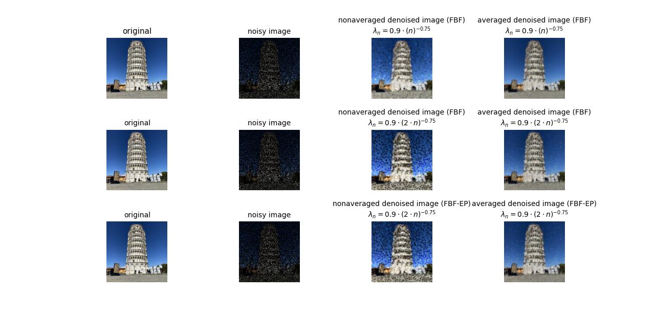
Figure 1: TV image inpainting was performed on four images, including the original image, an image with $80\%$ of its pixels missing, the non-averaged reconstructed image denoted as $x_{n}$, and the reconstructed image $z_{n}$ obtained after 2000 iterations using FBF and FBF-EP in the first and second row, respectively.

Figure 2 and 3 depict the evolution of the ISNR values for both the averaged and non-averaged reconstructed images using FBF and FBF-EP algorithms (in both two values of $\lambda_{n}$ in FBF, respectively). The theoretical outcomes concerning the sequences involved in Theorem 12 are illustrated in the figure, indicating that the averaged sequence exhibits better convergence properties than the non-averaged sequence. We notice that the behavior of ISNR values in both algorithms carry out similarly when we use the same value of $\lambda_{n}$ and the ISNR values of averaged FBF-EP have a bit outperform at 2000 iteration, even though we choose a bigger $\lambda_{n}$ in FBF for comparison. Table 1 reveals that the FBF-EP approach produced the best averaged reconstructed image with an ISNR value of 11.35116, while it was 11.32596 for the averaged case of the FBF with $\lambda_{n}=0.9(2\cdot n)^{-0.75}$ and 11.35073 for the averaged case of the FBF with $\lambda_{n}=0.9n^{-0.75}$ . However, the non-averaged reconstructed image using the FBF-EP method had the lowest ISNR value of 8.79544. Furthermore, the FBF-EP method was faster than the FBF method by around 15 seconds (compare with both two various of $\lambda_{n}$ in FBF), indicating that it can offer time-saving benefits in image reconstruction.

Remark 14.

1. During the computation, the construction of weighted averaged sequences, as defined in (5), requires the sequence $(x_{n})_{n\in\mathbb{N}\cup\{0\}}$ in every iterative step. Thus, we computed them simultaneously in our program and measured the time consumption.

2. The Python code is uploaded to the repository in GitHub. The reader can check it at the following link: https://github.com/BurisT/inpainting_python.

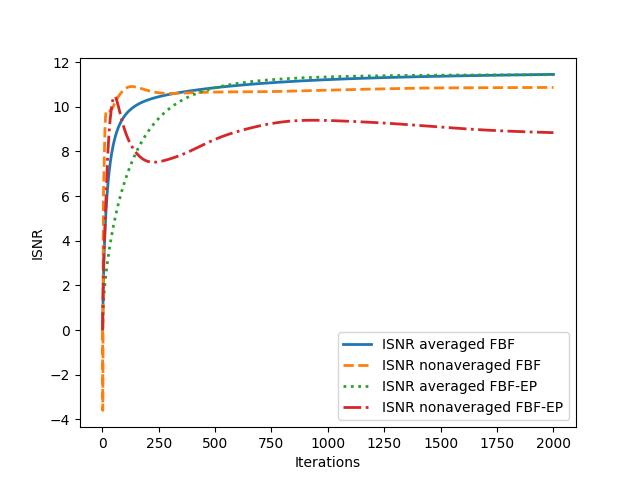
Figure 2: The figure illustrates the ISNR curves for both the averaged and non-averaged reconstructed images using the FBF method with $\lambda_{n}=0.9n^{-0.75}$ and FBF-EP with $\lambda_{n}=0.9(2\cdot n)^{-0.75}$ method.

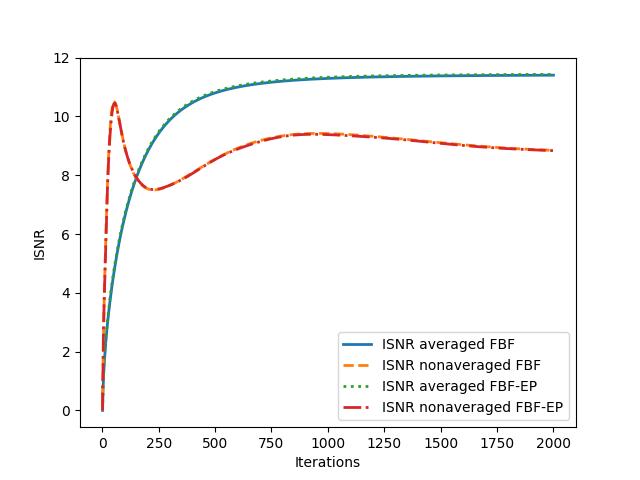
Figure 3: The figure illustrates the ISNR curves for both the averaged and non-averaged reconstructed images using the FBF and FBF-EP methods with the same value of $\lambda_{n}=0.9(2\cdot n)^{-0.75}$.

Acknowledgment. The Royal Government of Thailand scholarship through the Development and Promotion of Science and Technology Talents Project (DPST) provided funding for this work. The author is highly appreciative of Dr. habil. Ernö Robert Csetnek’s diligent direction.