The $q_{T}$ spectrum for Higgs production via heavy quark annihilation at N³LL^′+aN³LO

Abstract

We study the transverse momentum ($q_{T}$) spectrum of the Higgs boson produced via the annihilation of heavy quarks ($s,c,b$) in proton-proton collisions. Using soft-collinear effective theory (SCET) and working in the five-flavour scheme, we provide predictions at three-loop order in resummed perturbation theory (N³LL^′). We match the resummed calculation to full fixed-order results at next-to-next-to-leading order (NNLO), and introduce a decorrelation method to enable a consistent matching to an approximate N³LO (aN³LO) result. Since the $b$-quark initiated process exhibits large nonsingular corrections, it requires special care in the matching procedure and estimation of associated theoretical uncertainties, which we discuss in detail. Our results constitute the most accurate predictions to date for these processes in the small $q_{T}$ region and could be used to improve the determination of Higgs Yukawa couplings from the shape of the measured Higgs $q_{T}$ spectrum.

1 Introduction

With the discovery of the Higgs boson by the ATLAS and CMS experiments at the LHC [1, 2], the precise measurement of its properties has become essential to establish the Standard Model (SM) as the true mechanism of electroweak symmetry breaking. The four main production mechanisms – gluon fusion, vector boson fusion, Higgstrahlung, and top-quark pair associated production – have been observed experimentally [1, 2, 3, 4, 5], while the Higgs couplings to vector bosons have been found consistent with the SM down to an accuracy of $4\%$ [6, 7].

Probing the Higgs interactions with the fermionic sector is also of great importance. In the SM, the couplings of the Higgs boson to fermions, i.e. the Yukawa couplings $y_{F}$, are proportional to the fermion mass $m_{F}$, $y_{F}^{\mathrm{SM}}\equiv m_{F}/v$, where $v$ denotes the Higgs vacuum expectation value. This implies that the measurement of the Yukawa couplings to the heavy fermions is within the reach of the LHC. In fact, the reduced coupling strength factors $\kappa_{F}\equiv y_{F}/y_{F}^{\mathrm{SM}}$ have been measured to be $\kappa_{t}=0.92\pm 0.06$, $\kappa_{b}=0.88\pm 0.11$, and $\kappa_{\tau}=0.92\pm 0.07$ for the top-quark, bottom-quark, and $\tau$ lepton respectively [6, 7].

The bottom-quark Yukawa coupling $y_{b}$ is of particular interest. For example, in SM extensions such as the two Higgs doublet model or the minimally supersymmetric SM, $y_{b}$ can be enhanced relative to its SM value. This coupling has been measured in $H\to b\bar{b}$ decays [3, 8], which is challenging due to the required $b$ tagging and the huge multi-jet background. The same is true for the charm-quark Yukawa $y_{c}$, whose measurement from $H\to c\bar{c}$ decays is possible but presents an even greater challenge [9]. Therefore, a complementary determination of the Yukawa couplings stemming from the production process, rather than the decay, is of great interest.

In this work, we focus on Higgs production via quark annihilation $q\bar{q}\to H$, where we consider bottom, charm, and strange quarks for the incoming quarks. Of these, bottom-quark annihilation is by far the dominant process since the $b$ is the heaviest, followed by charm and then strange annihilation. Precise predictions for the $q\bar{q}\to H$ process are important, since it can in principle provide direct sensitivity to the quark Yukawa couplings from the production process. In addition, while the cross section for bottom-quark annihilation is significantly smaller than that of gluon fusion, these are often grouped together in experimental analyses, since they have very similar acceptances and are a priori hard to distinguish experimentally.

For these reasons, $q\bar{q}\to H$ production, in particular bottom-quark annihilation, has received much attention in the past, see e.g. refs. [10, 11, 12, 13, 14, 15, 16, 17, 18, 19, 20, 21, 22, 23, 24, 25, 26, 27, 28]. The $q\bar{q}H$ form factor and hard function have been computed up to four loops [29, 30], the total inclusive $b\bar{b}\to H$ cross section to N³LO [31, 32], and $b\bar{b}\to H+$jet to NNLO₁ [33].

The direct measurement of $b\bar{b}\to H$ by tagging one or both of the accompanying $b$-jets in the final state seems to be hopeless in practice [34]. Alternatively, one can exploit the pattern of QCD emissions from the incoming quarks and gluons to discriminate between the gluon and various quark channels in the initial state [35]. That is, the radiation pattern for different initial states yields different shapes for the transverse momentum ($q_{T}$) spectrum of the recoiling Higgs boson. As a result, a precise measurement and fit to the Higgs $q_{T}$ spectrum, especially at small $q_{T}$, allows one to gain sensitivity to the quark Yukawa couplings [36, 37]. With sufficient statistics, this might even open a way at the LHC to obtain some constraint on the strange Yukawa coupling (or more generally the PDF-weighted sum of light-quark Yukawa couplings).

In refs. [38, 39], ATLAS and CMS have demonstrated that it is already possible with existing data to obtain meaningful constraints on $\kappa_{c}$ and $\kappa_{b}$ from the shape of the Higgs $q_{T}$ spectrum alone. To fully exploit this possibility, a precise prediction of the $q_{T}$ spectrum for both gluon fusion and quark annihilation is essential. At small $q_{T}\ll m_{H}$, this requires the all-order resummation of logarithms of $q_{T}/m_{H}$ that would otherwise spoil the convergence of perturbation theory in this regime. While a N³LL^′+N³LO resummed prediction exists for the Higgs $q_{T}$ spectrum in gluon fusion [40], which was used in ref. [38], and predictions of similar accuracy also exist for Drell-Yan [41, 42, 43, 44, 45], no prediction of similar accuracy exists for $q\bar{q}\to H$, which so far has only been resummed to NNLL$+$NNLO accuracy [15, 20].

In this paper, we fill this gap and compute the resummed $q_{T}$ spectrum for $q\bar{q}\to H$ at N³LL^′ order matched to fixed NNLO and approximate N³LO. We use soft-collinear effective theory (SCET) [46, 47, 48, 49, 50] to resum the logarithms of $q_{T}/m_{H}$. We work in the limit $m_{q}\ll q_{T}$, where we only keep the Yukawa coupling of the annihilating quarks and otherwise take them to be massless. For $b\bar{b}\to H$, this is commonly referred to as the five-flavour scheme. Finite-mass effects become relevant for $m_{q}\sim q_{T}$ and are thus necessary for a complete description of the small-$q_{T}$ region, especially for $b\bar{b}\to H$ [15, 51]. Their full treatment in the resummed $q_{T}$ spectrum was worked out in ref. [51] and is quite involved. We therefore focus here on the massless limit and leave the inclusion of finite-mass effects in the resummed spectrum to future work.

This paper is organized as follows. We first provide a brief review of the structure of $q_{T}$ resummation in SCET in section 2, where we also discuss the general procedure for matching the resummed and fixed-order calculations using profile scales and for estimating perturbative uncertainties from profile-scale variations. In section 3, we discuss our implementation of the fixed-order results and the matching to them in some detail. It transpires that the numerical size of the nonsingular fixed-order corrections depends strongly on the incoming quark flavour. In particular, they are substantially larger for $b\bar{b}\to H$ than what is commonly found to be the case for gluon-fusion or Drell-Yan production. This requires additional care in the matching and some refinements to the usual estimation of the matching uncertainties based on profile-scale variations. Furthermore, we discuss the matching to approximate N³LO, i.e., to approximate $\mathcal{O}(\alpha_{s}^{3})$. For this purpose, we introduce a general strategy to decorrelate the singular and nonsingular contributions at large $q_{T}$, generalizing a method recently introduced in ref. [52]. This allows us to construct an approximation of the missing $\mathcal{O}(\alpha_{s}^{3})$ nonsingular contributions and a corresponding approximate full NNLO₁ result that incorporates the exact $\mathcal{O}(\alpha_{s}^{3})$ singular contributions, which are neccessary for a consistent matching to the N³LL^′ result. We present our numerical results for the resummed $q_{T}$ spectrum and its perturbative uncertainties in section 4, and offer avenues for potential future work in section 5.

2 Theoretical framework

2.1 Factorization and resummation

We consider the cross section for an on-shell Higgs boson differential in the Higgs rapidity $Y$ and Higgs transverse momentum ${\vec{q}}_{T}$. At small $q_{T}\equiv|{\vec{q}}_{T}|\ll m_{H}$, we can expand the cross section in powers of $q_{T}^{2}/m_{H}^{2}$ as

$$\frac{\mathrm{d}\sigma}{\mathrm{d}Y\mathrm{d}^{2}{\vec{q}}_{T}} =\frac{\mathrm{d}\sigma^{\mathrm{sing}}}{\mathrm{d}Y\mathrm{d}^{2}{\vec{q}}_{T}}+\frac{\mathrm{d}\sigma^{\mathrm{nons}}}{\mathrm{d}Y\mathrm{d}^{2}{\vec{q}}_{T}}=\frac{\mathrm{d}\sigma^{\mathrm{sing}}}{\mathrm{d}Y\mathrm{d}^{2}{\vec{q}}_{T}}\biggl{[}1+\mathcal{O}\Bigl{(}\frac{q_{T}^{2}}{m_{H}^{2}}\Bigr{)}\biggr{]}\,.$$ (2.1)

Here, $\mathrm{d}\sigma^{\mathrm{sing}}$ contains the leading-power “singular” contributions in the $q_{T}\to 0$ limit involving $\delta(q_{T})$ distributions and logarithmic plus distributions $[\ln^{n}(q_{T}/m_{H})/q_{T}]_{+}$. All remaining “nonsingular” contributions, which are suppressed by $\mathcal{O}(q_{T}^{2}/m_{H}^{2})$ relative to $\mathrm{d}\sigma^{\mathrm{sing}}$, are contained in $\mathrm{d}\sigma^{\mathrm{nons}}$.

The factorization of the leading-power $q_{T}$ spectrum was first established by Collins, Soper, and Sterman [53, 54, 55], and was further elaborated upon and extended in refs. [56, 57, 58]. In this work we employ the framework of SCET, in which $q_{T}$ factorization was formulated in refs. [59, 60, 61, 62], and which is equivalent to the modern formulation in ref. [58]. We employ the rapidity renormalization group [61] together with the exponential regulator from ref. [62] for which the ingredients required for the resummation at N³LL^′ are known. Up to two loops it yields the same results as the $\eta$ regulator used in ref. [61]. In this formulation, the singular cross section can be written in factorized form as

$$\frac{\mathrm{d}\sigma^{\mathrm{sing}}}{\mathrm{d}Y\mathrm{d}^{2}{\vec{q}}_{T}} =\sum_{a,b}H_{ab}(m_{H}^{2};\mu)[B_{a}\otimes B_{b}\otimes S_{ab}](x_{a},x_{b},{\vec{q}}_{T};\mu)\,,$$ (2.2)

where the kinematic quantities $\omega_{a,b}$ and $x_{a,b}$ are given by

$$\omega_{a}=m_{H}e^{+Y},\quad\omega_{b}=m_{H}e^{-Y}\quad\text{ and}\quad\quad x_{a,b}=\frac{\omega_{a,b}}{E_{\mathrm{cm}}}\,.$$ (2.3)

The process dependence is encoded in the hard function $H_{ab}(m_{H}^{2},\mu)$. It describes the underlying hard interaction producing the Higgs boson via $ab\to H$, with the available partonic channels being $ab=\{{q\bar{q},\,{\bar{q}q}}\}$. At leading order, $H^{(0)}$ corresponds to the partonic Born squared matrix element, while at higher orders it includes the finite virtual corrections to the Born process.

The factor $[B_{a}\otimes B_{b}\otimes S_{ab}]$ in eq. (2.2) describes physics at the low scale $\mu\sim q_{T}$ and is defined as the following convolution in ${\vec{q}}_{T}$:

$$[B_{a}\otimes B_{b}\otimes S_{ab}](x_{a},x_{b},{\vec{q}}_{T};\mu) \equiv\int\!\mathrm{d}^{2}\vec{k}_{a}\,\mathrm{d}^{2}\vec{k}_{b}\,\mathrm{d}^{2}\vec{k}_{s}\,\delta^{2}({\vec{q}}_{T}-\vec{k}_{a}-\vec{k}_{b}-\vec{k}_{s})$$ (2.4)

$$\qquad\times B_{a}(x_{a},\vec{k}_{a};\mu,\nu/\omega_{a})\,B_{b}(x_{b},\vec{k}_{b};\mu,\nu/\omega_{b})\,S_{ab}(\vec{k}_{s};\mu,\nu)\,.$$

The functions in eq. (2.4) are universal objects in ${\vec{q}}_{T}$ factorization, independent of the details of the hard process. They are renormalized, with $\mu$ and $\nu$ denoting their virtuality and rapidity renormalization scales. The beam functions $B_{a,b}$ describe collinear radiation with total transverse momentum $\vec{k}_{a,b}$ and longitudinal momentum $\omega_{a,b}$, while the soft function $S_{ab}$ describes soft radiation with total transverse momentum $\vec{k}_{s}$. Momentum conservation in the transverse plane implies that the sum of $\vec{k}_{a}$, $\vec{k}_{b}$, $\vec{k}_{s}$ must be equal to the measured Higgs transverse momentum ${\vec{q}}_{T}$, leading to the convolution structure in eq. (2.4).

In Fourier-conjugate ${\vec{b}}_{T}$ space, the convolutions in ${\vec{q}}_{T}$ in eq. (2.4) turn into simple products. The factorized singular cross section in ${\vec{b}}_{T}$ space then takes the form

$$\frac{\mathrm{d}\tilde{\sigma}^{\mathrm{sing}}(\vec{b}_{T})}{\mathrm{d}Y} \equiv\int\!\frac{\mathrm{d}^{2}{\vec{q}}_{T}}{(2\pi)^{2}}\,e^{-\mathrm{i}\,{\vec{q}}_{T}\cdot{\vec{b}}_{T}}\,\frac{\mathrm{d}\sigma^{\mathrm{sing}}}{\mathrm{d}Y\mathrm{d}^{2}{\vec{q}}_{T}}$$

$$=\sum_{a,b}H_{ab}(m_{H}^{2};\mu)\tilde{B}_{a}(x_{a},{\vec{b}}_{T};\mu,\nu/\omega_{a})\,\tilde{B}_{b}(x_{b},{\vec{b}}_{T};\mu,\nu/\omega_{b})\,\tilde{S}_{ab}(b_{T};\mu,\nu)\,,$$ (2.5)

where $\tilde{B}_{a,b}$ and $\tilde{S}_{ab}$ are the Fourier transforms of $B_{a,b}$ and $S_{ab}$ appearing in eq. (2.4).

To perform all-order resummation, each function is first evaluated at its own natural boundary scale(s): $\mu_{H}$, $(\mu_{B},\nu_{B})$, and $(\mu_{S},\nu_{S})$. By choosing appropriate values for the boundary scales close to their canonical values (see section 2.2), each function is free of large logarithms and can therefore be evaluated in fixed-order perturbation theory. Next, all functions are evolved from their respective boundary conditions to a common arbitary point $(\mu,\nu)$ by solving their coupled system of renormalization group equations (RGEs). The RGEs are themselves multiplicative in ${b}_{T}$ space and convolutions in ${\vec{q}}_{T}$ space. For more details we refer to refs. [63, 64].

	Boundary	Anomalous dimensions		FO matching
Order	conditions	$\gamma_{i}$ (noncusp)	$\Gamma_{\mathrm{cusp}}$, $\beta$	(nonsingular)
LL	$1$	-	1-loop	-
NLL	$1$	1-loop	2-loop	-
NLL′ $(+$NLO$)$	$\alpha_{s}$	1-loop	2-loop	$\alpha_{s}$
NNLL $(+$NLO$)$	$\alpha_{s}$	2-loop	3-loop	$\alpha_{s}$
NNLL′ $(+$NNLO$)$	$\alpha_{s}^{2}$	2-loop	3-loop	$\alpha_{s}^{2}$
N3LL $(+$NNLO$)$	$\alpha_{s}^{2}$	3-loop	4-loop	$\alpha_{s}^{2}$
N3LL′ $(+$N3LO$)$	$\alpha_{s}^{3}$	3-loop	4-loop	$\alpha_{s}^{3}$
N4LL $(+$N3LO$)$	$\alpha_{s}^{3}$	4-loop	5-loop	$\alpha_{s}^{3}$

Table 1: Definition of resummation orders. The $(+$NⁿLO$)$ in the order refers to whether or not the nonsingular $\mathcal{O}(\alpha_{s}^{n})$ corrections in the last column are included.

The resummation order is defined by the $\alpha_{s}$ and loop orders to which the boundary conditions and anomalous dimensions entering the RGE are included, as summarized in table 1. For the resummation at N³LL^′ we require the N³LO boundary conditions for the hard function [29, 65], and the beam and soft functions [66, 67, 68, 69, 70]. We also need the 3-loop noncusp virtuality [66, 71, 72, 73, 68] and rapidity anomalous dimensions [66, 67, 74], as well as the 4-loop cusp anomalous dimension $\Gamma_{\mathrm{cusp}}$ [75, 76, 77, 78, 79] and QCD $\beta$ function [80, 81, 82, 83].

2.2 Canonical scales and resummation in $b_{T}$ space

The canonical boundary scales in $b_{T}$ space are given by

virtuality: $$\quad\mu_{H}=m_{H},\quad\mu_{B}=b_{0}/b_{T},\quad\mu_{S}=b_{0}/b_{T},\quad\mu_{f}=b_{0}/b_{T},\quad\mu_{0}=b_{0}/b_{T},$$

rapidity: $$\hskip 75.39963pt\nu_{B}=m_{H},\,\hskip 18.77892pt\nu_{S}=b_{0}/b_{T}\,,$$ (2.6)

where $b_{0}\equiv 2e^{-\gamma_{E}}\approx 1.12291$. Here, $\mu_{H}$, $(\mu_{B},\nu_{B})$, and $(\mu_{S},\nu_{S})$ are the boundary scales for the hard, beam, and soft functions, and $\mu_{f}$ is the scale at which the PDFs inside the beam functions are evaluated. The rapidity anomalous dimension must also be resummed and $\mu_{0}$ is its associated boundary scale. When the functions in eq. (2.1) are evolved from these scales, the evolution resums all canonical $b_{T}$-space logarithms $\ln^{n}[(b_{0}/b_{T})/m_{H}]$.

As shown in ref. [63], the exact solution for the RG evolution in ${\vec{q}}_{T}$ space in terms of distributions is equivalent to this canonical solution in $b_{T}$ space modulo different conventions for the boundary conditions. Since the latter is much easier to obtain, we also use it here, as is often done. The resummed singular ${\vec{q}}_{T}$ spectrum, $\mathrm{d}\sigma^{\mathrm{res}}$, is then obtained as the inverse Fourier transform of the canonically resummed $b_{T}$ space result, $\mathrm{d}\tilde{\sigma}^{\mathrm{res}}({\vec{b}}_{T})$,

$$\frac{\mathrm{d}\sigma^{\mathrm{res}}}{\mathrm{d}Y\mathrm{d}^{2}{\vec{q}}_{T}} =\int\!\mathrm{d}^{2}{\vec{b}}_{T}\,e^{\mathrm{i}\,{\vec{q}}_{T}\cdot{\vec{b}}_{T}}\,\frac{\mathrm{d}\tilde{\sigma}^{\mathrm{res}}(\vec{b}_{T})}{\mathrm{d}Y}=2\pi\int\!\mathrm{d}b_{T}\,b_{T}J_{0}(b_{T}q_{T})\,\frac{\mathrm{d}\tilde{\sigma}^{\mathrm{res}}(\vec{b}_{T})}{\mathrm{d}Y}\,.$$ (2.7)

With the canonical scales in eq. (2.2), the strong coupling and the PDFs inside the beam functions are evaluated at $\alpha_{s}(b_{0}/b_{T})$, which means the beam and soft functions and rapidity anomalous dimension become sensitive to nonperturbative effects for $1/b_{T}\lesssim\Lambda_{\mathrm{QCD}}$. To perform the Fourier transform in eq. (2.7), we must therefore choose a prescription to avoid such nonperturbative scales.

The traditional approach is to perform a global replacement of $b_{T}$ everywhere in the $b_{T}$-space cross section by a function $b^{*}(b_{T})$, which asymptotes to some fixed perturbative scale $b_{\mathrm{max}}\lesssim 1/\Lambda_{\mathrm{QCD}}$ for $1/b_{T}\to 0$, while away from this limit it becomes $b_{T}$. An important drawback of this global $b^{*}$ prescription is that it leads to much larger than necessary distortions of the $b_{T}$-space cross section. This can be avoided by applying this replacement only to the canonical scale choices [84], which suffices to avoid nonperturbative scales. More precisely, following ref. [45], we use the $\mu_{*}$ prescription

$$\mu_{X}=\mu_{*}\bigl{(}b_{0}/b_{T},\mu_{X}^{\mathrm{min}}\bigr{)}\quad\text{with}\quad\mu_{*}(x,y)=\sqrt{x^{2}+y^{2}}\,,$$ (2.8)

where $\mu_{X}$ stands for any of $\mu_{S}$, $\mu_{B}$, $\mu_{0}$, $\mu_{f}$. In principle any function $\mu_{*}(x,y)$ can be used which satisfies $\mu_{*}(x\to 0,y)\to y$ and $\mu_{*}(x\gg y,y)\to x$. Under these conditions, all scales approach their chosen minimum value $\mu_{X}^{\mathrm{min}}$ for $1/b_{T}\to 0$, while approaching their canonical values away from this limit, as desired. Note that one advantage of this prescription is that we have the option to choose different $\mu_{X}^{\mathrm{min}}$ values for different scales, which we will make use of for $\mu_{f}$.

2.3 Profile scales and matching to fixed order

In addition to the leading-power contributions, which are resummed with the help of the factorization theorem in eqs. (2.2) and (2.4), we also have to include the nonsingular power corrections $\mathrm{d}\sigma^{\mathrm{nons}}$ in eq. (2.1). To do so, we add them to the resummed singular contributions to obtain the final matched result

$$\mathrm{d}\sigma =\mathrm{d}\sigma^{\mathrm{res}}(\mu_{\mathrm{res}})+\mathrm{d}\sigma^{\mathrm{nons}}(\mu_{\mathrm{FO}})$$

$$=\mathrm{d}\sigma^{\mathrm{res}}(\mu_{\mathrm{res}})+\Bigl{[}\mathrm{d}\sigma^{\mathrm{FO}}(\mu_{\mathrm{FO}})-\mathrm{d}\sigma^{\mathrm{sing}}(\mu_{\mathrm{FO}})\Bigr{]}\,.$$ (2.9)

The first line is equivalent to eq. (2.1), using the all-order resummed result $\mathrm{d}\sigma^{\mathrm{res}}(\mu_{\mathrm{res}})$ for the singular contributions. We use the $\mu_{\mathrm{res}}$ argument here to indicate that $\mathrm{d}\sigma^{\mathrm{res}}$ is evaluated using the resummation (boundary) scales as discussed in section 2.2. The nonsingular cross section $\mathrm{d}\sigma^{\mathrm{nons}}(\mu_{\mathrm{FO}})$ is included at fixed order, with its $\mu_{\mathrm{FO}}$ argument indicating that it is evaluated at the fixed-order scales (the usual $\mu_{R}$ and $\mu_{F}$). It is obtained as shown in the second line in eq. (2.3), i.e. by using eq. (2.1) at fixed order and subtracting the fixed-order singular terms from the full fixed-order result, where (as indicated) both are evaluated at common fixed-order scales $\mu_{\mathrm{FO}}$. This subtraction can be done directly in momentum space.

For small $q_{T}\ll m_{H}$, the nonsingular terms are a small power correction and it is sufficient to include them at fixed order despite the fact that the singular terms are resummed there. For the nonsingular to be indeed power suppressed it is essential that $\mathrm{d}\sigma^{\mathrm{FO}}$ and $\mathrm{d}\sigma^{\mathrm{sing}}$ are evaluated at the same fixed order, such that $\mathrm{d}\sigma^{\mathrm{sing}}$ exactly contains and cancels the singular terms of $\mathrm{d}\sigma^{\mathrm{FO}}$.

On the other hand, as $q_{T}$ approaches $q_{T}\sim m_{H}$, the distinction between singular and nonsingular becomes arbitrary and only the full fixed-order result in $\mathrm{d}\sigma^{\mathrm{FO}}$ is physically meaningful. To recover the correct $\mathrm{d}\sigma^{\mathrm{FO}}$ in this limit, $\mathrm{d}\sigma^{\mathrm{res}}(\mu_{\mathrm{res}})$ and $\mathrm{d}\sigma^{\mathrm{sing}}(\mu_{\mathrm{FO}})$ must cancel each other in eq. (2.3). We require this cancellation to be exact with no leftover higher-order terms in $\alpha_{s}$, because for $q_{T}\sim m_{H}$ the (resummed) singular terms are unphysical and typically become numerically much larger than the actual physical result given by $\mathrm{d}\sigma^{\mathrm{FO}}$. This requires the turning off of the resummation in $\mathrm{d}\sigma^{\mathrm{res}}(\mu_{\mathrm{res}})$ – in so doing, one guarantees that the result becomes equal to the fixed-order $\mathrm{d}\sigma^{\mathrm{sing}}(\mu_{\mathrm{FO}})$. Considering the first line of eq. (2.3), this implies that for $q_{T}\sim m_{H}$ there are typically large numerical cancellations between the singular and nonsingular contributions.

In summary, in order to have a consistent description of the cross section for all values of $q_{T}$, the terms in eq. (2.3) are required to satisfy two conditions: firstly, $\mathrm{d}\sigma^{\mathrm{sing}}$ and $\mathrm{d}\sigma^{\mathrm{FO}}$ must be evaluated at the same fixed order; secondly, $\mathrm{d}\sigma^{\mathrm{sing}}$ and $\mathrm{d}\sigma^{\mathrm{res}}$ must become equal in the limit where the resummation in $\mathrm{d}\sigma^{\mathrm{res}}$ is turned off.

The most natural way to turn off the resummation in $\mathrm{d}\sigma^{\mathrm{res}}(\mu_{\mathrm{res}})$ is to set all boundary scales to the common fixed-order scales $\mu_{\mathrm{FO}}$, i.e. in our notation $\mu_{\mathrm{res}}=\mu_{\mathrm{FO}}$. The second condition above thus requires $\mathrm{d}\sigma^{\mathrm{res}}(\mu_{\mathrm{res}}=\mu_{\mathrm{FO}})=\mathrm{d}\sigma^{\mathrm{sing}}(\mu_{\mathrm{FO}})$. The first condition above then requires for a given resummation order a specific order for the nonsingular matching corrections. Namely, the $\alpha_{s}$ order of the boundary conditions in the resummed result must match the $\alpha_{s}$ order of the full and nonsingular results, which are the orders shown in the last column of table 1.

In practice, we want to turn off the resummation smoothly, such that the difference $\mathrm{d}\sigma^{\mathrm{res}}(\mu_{\mathrm{res}})-\mathrm{d}\sigma^{\mathrm{sing}}(\mu_{\mathrm{FO}})$ vanishes equally smoothly as $q_{T}\to m_{H}$. This is conveniently achieved by using profile scales [85, 86], which provide a smooth transition for $\mu_{\mathrm{res}}$ from canonical resummation scales to the common fixed-order scales. Here we use hybrid profile scales $\mu_{X}(b_{T},q_{T})$ [84], which depend on both $b_{T}$ and $q_{T}$ and undergo a smooth transition from their canonical $b_{T}$-dependence in eq. (2.8) to the $b_{T}$-independent $\mu_{\mathrm{FO}}$, with the transition happening as a function of $q_{T}$,

$$\mu_{X}(b_{T},q_{T}) =\mu_{*}\bigl{(}b_{0}/b_{T},\mu_{X}^{\mathrm{min}}\bigr{)}\quad \text{for}\quad q_{T}\ll m_{H}\,,$$

$$\mu_{X}(b_{T},q_{T}) \to\mu_{\mathrm{FO}}\quad \text{for}\quad q_{T}\to m_{H}\,.$$ (2.10)

We choose the central scales as

$$\mu_{H}=\nu_{B}=\mu_{\mathrm{FO}} =m_{H}\,,$$

$$\mu_{X} =m_{H}\,f_{\mathrm{run}}\Bigl{[}\frac{q_{T}}{m_{H}},\frac{1}{m_{H}}\mu_{*}\Bigl{(}\frac{b_{0}}{b_{T}},\mu_{X}^{\mathrm{min}}\Bigr{)}\Bigr{]}\qquad\text{for}\quad\mu_{X}\in\{\mu_{B},\mu_{S},\nu_{S},\mu_{f}\}\,,$$

$$\mu_{0} =\mu_{*}\Bigl{(}\frac{b_{0}}{b_{T}},\mu_{0}^{\mathrm{min}}\Bigr{)}\,,$$ (2.11)

where $f_{\mathrm{run}}$ is the hybrid profile function given by [84]

$$f_{\mathrm{run}}(x,y) =1+g_{\mathrm{run}}(x)(y-1)\,,$$ (2.12)

where $g_{\mathrm{run}}(x)$ determines the transition as a function of $x=q_{T}/m_{H}$,

$$g_{\mathrm{run}}(x) =\begin{cases}1&0<x\leq x_{1}\,,\\ 1-\frac{(x-x_{1})^{2}}{(x_{2}-x_{1})(x_{3}-x_{1})}&x_{1}<x\leq x_{2}\,,\\ \frac{(x-x_{3})^{2}}{(x_{3}-x_{1})(x_{3}-x_{2})}&x_{2}<x\leq x_{3}\,,\\ 0&x_{3}\leq x\,,\end{cases}$$ (2.13)

with the transition points $x_{i}$ with $i\in\{1,2,3\}$. The parameters $x_{1}$ and $x_{3}$ determine the start and end of the transition and $x_{2}=(x_{1}+x_{3})/2$ corresponds to the turning point. As a result the scales are canonical for $q_{T}\leq x_{1}m_{H}$ and the resummation is fully turned off for $q_{T}>x_{3}\,m_{H}$. The values are usually chosen such that the transition begins somewhere in the resummation region and is finished by the time the singular and the nonsingular contributions are of the same size and exhibit sizeable numerical cancellations. We will use $[x_{1},x_{2},x_{3}]=[0.1,0.45,0.8]$ as our central values as explained in section 3.2.

For the $\mu_{X}^{\mathrm{min}}$ nonperturbative cutoffs we use

$$\mu_{B}^{\mathrm{min}}=\mu_{S}^{\mathrm{min}}=\mu_{0}^{\mathrm{min}}=1\,\mathrm{GeV}\,,\qquad\nu_{S}^{\mathrm{min}}=0\,.$$ (2.14)

We can set $\nu_{S}^{\mathrm{min}}=0$ because $\nu_{S}$ never appears as argument of $\alpha_{s}$ or the PDFs. For $\mu_{f}^{\mathrm{min}}$ we pick the larger of the PDF’s $Q_{0}$ value or a value based on the quark mass $m_{q}$ used by the PDF set as threshold for the corresponding heavy-quark PDF. This choice of $\mu_{f}^{\mathrm{min}}$ avoids running into numerical noise below the scale where the heavy-quark PDFs vanish and where the results are in any case not particularly meaningful without the proper inclusion of finite-mass effects, which is beyond our scope here. For the MSHT20nnlo PDF set we use, this amounts to taking $\mu_{f}^{\mathrm{min}}=Q_{0}=1.0\,\mathrm{GeV}$ for $s\bar{s}\to H$, $\mu_{f}^{\mathrm{min}}=m_{c}=1.4\,\mathrm{GeV}$ for $c\bar{c}\to H$ and $\mu_{f}^{\mathrm{min}}=5.0\,\mathrm{GeV}$ for $b\bar{b}\to H$. The latter is chosen slightly above the actual bottom-quark mass threshold $m_{b}=4.75\,\mathrm{GeV}$ to avoid numerical instabilities.

In the fixed-order limit, we can identify $\mu_{\mathrm{FO}}\equiv\mu_{R}$ with the usual renormalization scale for $\alpha_{s}$ and $\mu_{f}\equiv\mu_{F}$ with the usual factorization scale at which the PDFs are evaluated. Our central choices above correspond to $\mu_{R}=\mu_{F}=m_{H}$.

2.4 Perturbative uncertainties

To estimate the perturbative uncertainties, we vary the profile scales about their central values given in section 2.3. Following refs. [87, 64, 45], we identify several different sources of uncertainty, which are considered as independent and are estimated from different suitable types of variations. The profile scales are varied as follows:

$$\mu_{H} =\mu_{\mathrm{FO}}=2^{w_{\mathrm{FO}}}\,m_{H}\,,$$

$$\nu_{B} =\mu_{\mathrm{FO}}\,f_{\mathrm{vary}}^{v_{\nu_{B}}}\Bigl{(}\frac{q_{T}}{m_{H}}\Bigr{)}\,,$$

$$\mu_{X} =\mu_{\mathrm{FO}}\,f_{\mathrm{vary}}^{v_{\mu_{X}}}\Bigl{(}\frac{q_{T}}{m_{H}}\Bigr{)}f_{\mathrm{run}}\biggl{[}\frac{q_{T}}{m_{H}},\frac{1}{m_{H}}\mu_{*}\Bigl{(}\frac{b_{0}}{b_{T}},\frac{\mu_{X}^{\mathrm{min}}}{2^{w_{\mathrm{FO}}}f_{\mathrm{vary}}^{v_{\mu_{X}}}}\Bigr{)}\biggr{]}\quad\text{for}\quad\mu_{X}\in\{\mu_{B},\mu_{S},\nu_{S}\}\,,$$

$$\mu_{f} =2^{w_{F}}\,m_{H}\,f_{\mathrm{run}}\biggl{[}\frac{q_{T}}{m_{H}},\frac{1}{m_{H}}\mu_{*}\Bigl{(}\frac{b_{0}}{b_{T}},\frac{\mu_{f}^{\mathrm{min}}}{2^{w_{F}}}\Bigr{)}\biggr{]}\,,$$

$$\mu_{0} =\mu_{*}\Bigl{(}\frac{b_{0}}{b_{T}},\mu_{0}^{\mathrm{min}}\Bigr{)}\,.$$ (2.15)

To estimate an uncertainty associated with the resummation $\Delta_{\mathrm{res}}$, the beam and soft scales are varied, where the exponents $v_{\mu_{B}}$, $v_{\nu_{B}}$, $v_{\mu_{S}}$, and $v_{\nu_{S}}$ are taken to be $v_{i}=\{-1,0,+1\}$ with the central scales corresponding to $v_{i}=0$. The function

$$f_{\mathrm{vary}}(x) =\begin{cases}2(1-x^{2}/x_{3}^{2})&0\leq x\leq x_{3}/2\,,\\ 1-2(1-x/x_{3})^{2}&x_{3}/2<x\leq x_{3}\,,\\ 1&x_{3}\leq x\,,\end{cases}$$ (2.16)

with $x\equiv q_{T}/m_{H}$ controls the size of the variations, ranging from a factor of 2 for $x=0$ to 1 for $x\geq x_{3}$, where $x_{3}$ is the same as for $f_{\mathrm{run}}(x)$. This source of uncertainty is thus turned off for $q_{T}\geq x_{3}m_{H}$ just as the resummation itself is turned off. To estimate the resulting resummation uncertainty $\Delta_{\mathrm{res}}$ we perform 36 variations of suitable combinations of the $v_{i}$ and take their maximum envelope. For details, we refer the reader to ref. [64].

For the fixed-order uncertainty $\Delta_{\mathrm{FO}}$, we vary $\mu_{\mathrm{FO}}$ by a factor of 2 by taking $w_{\mathrm{FO}}=\{-1,0,+1\}$ everywhere. Note that $\Delta_{\mathrm{FO}}$ is not defined to be the uncertainty in the fixed-order limit but is rather meant to estimate a common uncertainty due to missing fixed-order contributions at any $q_{T}$. It therefore contributes to both the singular and nonsingular pieces. In the resummed singular it amounts to an overall variation of the boundary scales such that the resummed logarithms are unchanged, which is why one can interpret it as a fixed-order uncertainty. Furthermore, we estimate a separate uncertainty $\Delta_{\mu_{f}}$ related to the DGLAP running of the PDFs, for which we vary the PDF scale $\mu_{f}$ by taking $w_{F}=\{-1,0,+1\}$ (where $w_{F}=0$ is the central value). In the nonsingular and full fixed-order cross sections, this corresponds to taking $\mu_{f}\equiv\mu_{F}=2^{w_{F}}m_{H}$. The resulting $\Delta_{\mathrm{FO}}$ and $\Delta_{\mu_{f}}$ are then given by the maximum envelope of the respective variations.

We obtain the total perturbative uncertainty by adding the individual uncertainties in quadrature,

$$\Delta_{\mathrm{total}}=\sqrt{\Delta_{\mathrm{FO}}^{2}+\Delta_{\mathrm{res}}^{2}+\Delta_{\mu_{f}}^{2}+\Delta^{2}_{\mathrm{match}}}.$$ (2.17)

The matching uncertainty $\Delta_{\mathrm{match}}$ will be discussed in section 3.2.

Note that in the fixed-order limit, we do not use an envelope of $\mu_{R}$ and $\mu_{F}$ variations as is commonly done. Instead, we estimate separate uncertainties $\Delta_{\mathrm{FO}}$ and $\Delta_{\mu_{f}}$ which are added in quadrature. By separating these two uncertainties in the resummation limit, we essentially have no choice but to do the same also at fixed order. This is not problematic, but is in fact a perfectly sensible choice for the fixed-order prediction – here, as in the resummation, the two variations probe two conceptually different sources of uncertainty.

3 Fixed-order contributions and matching at aN³LO

In this section, we discuss several aspects specific to the $q\bar{q}\to H$ process we are interested in here. In section 3.1, we describe our implementation and validation of the fixed-order calculation for the $q\bar{q}\to H+j$ process from which we obtain the nonsingular corrections. In section 3.2, we discuss how we choose the transition points for the profile function in eq. (2.13), and detail the procedure to estimate the associated matching uncertainty, which is particularly delicate for $b\bar{b}\to H$. In section 3.3, we describe a general strategy to decorrelate the singular and nonsingular contributions. Based on this, we construct in section 3.4 a suitable approximation for the fixed $\mathcal{O}(\alpha_{s}^{3})$ corrections to the nonsingular and full cross sections.

3.1 Fixed-order calculations

As discussed in section 2.3, the nonsingular corrections are obtained at fixed order by taking

$$\frac{\mathrm{d}\sigma^{\mathrm{nons}}}{\mathrm{d}q_{T}} =\frac{\mathrm{d}\sigma^{\mathrm{FO}}}{\mathrm{d}q_{T}}-\frac{\mathrm{d}\sigma^{\mathrm{sing}}}{\mathrm{d}q_{T}}\,,$$ (3.1)

where $\mathrm{d}\sigma^{\mathrm{sing}}$ is obtained directly in momentum space from the fixed-order expansion of the factorization theorem in eq. (2.2). Since $\mathrm{d}\sigma^{\mathrm{nons}}$ is power suppressed, we only need it for $q_{T}>0$. Hence, to evaluate $\mathrm{d}\sigma^{\mathrm{FO}}$ we require the fixed-order calculation for the $q_{T}$ spectrum in $q\bar{q}\to H+j$. At N³LL^′ we need $\mathrm{d}\sigma^{\mathrm{FO}}$ at $\mathcal{O}(\alpha_{s}^{3})$ corresponding to the $q\bar{q}\to H+j$ calculation at NNLO₁ (the subscript $1$ on the order counting indicates that it is relative to the $H+1$-parton cross section).

3.1.1 LO₁ and NLO₁

For the lowest order, LO₁, we have performed an analytic calculation, which we have implemented in SCETlib [88] – the relevant details are provided for completeness in appendix A. For the NLO₁ calculation, we use a parton-level Monte Carlo calculation, which we have implemented in the Geneva event generator [89, 90] using FKS subtractions [91]. We have used the virtual matrix elements in analytic form, which were calculated in ref. [92] and implemented in the Geneva code in ref. [93]. The tree-level double-real emission matrix elements are obtained from the OpenLoops library [94]. Note that often only the $b\bar{b}\to H$ process is considered. We therefore performed several internal cross checks to also ensure the correct implementation of $c\bar{c}\to H+j$ and $s\bar{s}\to H+j$. At LO₁, we also checked the implementation against our analytic implementation in SCETlib.

A powerful cross check of the fixed-order calculation is provided by the cancellation of all singular terms in the $q_{T}\to 0$ limit in eq. (3.1). This is shown for both the $\mathcal{O}(\alpha_{s})$ and $\mathcal{O}(\alpha_{s}^{2})$ corrections in figure -1199. In both cases, the full (blue) and singular (red) results become essentially equal for small $q_{T}$, and the nonsingular (green) given by their difference exhibits the expected power suppression. Note that these plots show $|\mathrm{d}\sigma/\mathrm{d}\log_{10}q_{T}|$ on a log-log scale, for which an $\mathcal{O}(q_{T}^{2}/m_{H}^{2})$ power suppression corresponds to a line with an asymptotic slope of $-2$ for $q_{T}\to 0$. This is clearly seen at $\mathcal{O}(\alpha_{s})$. At $\mathcal{O}(\alpha_{s}^{2})$ this is less apparent due to the limited Monte-Carlo integration precision at very small $q_{T}$ and because the nonsingular contribution contains powers of logarithms $\ln^{n}(q_{T}^{2}/m_{H}^{2})$ up to $n\leq 3$, which weaken the power supression and effectively delay the strictly quadratic scaling to smaller $q_{T}$. We nevertheless observe a clear power suppression from around 30 GeV down to a few GeV until the numerical precision becomes insufficient to actually resolve the small but nonzero value of the nonsingular. Note that once this happens, the result for the nonsingular should fluctuate around and be consistent with zero within the statistical uncertainties. This is confirmed in figure -1198, which shows the nonsingular from figure -1199 but on a linear $y$ axis and including the sign. Analogous results for $c\bar{c}\to H$ and $s\bar{s}\to H$ are provided in appendix B.

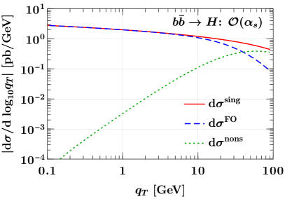
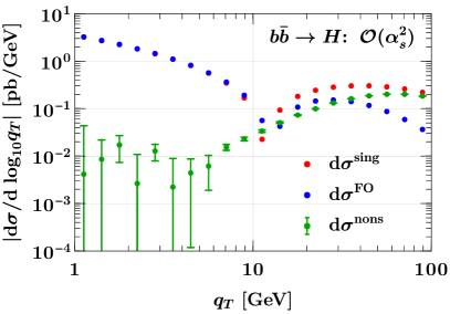
Figure -1199: Singular (solid red), full (dashed blue), and nonsingular (dotted green) contributions for $b\bar{b}\to H$ at fixed $\mathcal{O}(\alpha_{s})$ (left) and $\mathcal{O}(\alpha_{s}^{2})$ (right). The nonsingular exhibit the expected quadratic power suppression for $q_{T}\to 0$.

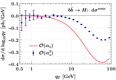
Figure -1198: Nonsingular contributions at $\mathcal{O}(\alpha_{s})$ (red) and $\mathcal{O}(\alpha_{s}^{2})$ for $b\bar{b}\to H$ on a linear scale, corresponding respectively to the green curves and points in figure -1199.

3.1.2 NNLO₁

A calculation for $b\bar{b}\to H+j$ has been achieved at NNLO₁ in ref. [33] using $N$-jettiness subtractions [95, 96]. This calculation uses a cut on the jet-$p_{T}\geq 30\,\mathrm{GeV}$, which gives an unbiased result for the $q_{T}$ spectrum only for $q_{T}\geq 60\,\mathrm{GeV}$. The jet-$p_{T}$ cut limits the size of residual power corrections in the $N$-jettiness slicing parameter, which scale with the inverse of the smallest kinematic scale in the process. It would require substantial high-performance computing resources to perform the full NNLO₁ calculation without a jet cut down to much smaller $q_{T}$ (this is also what experience has shown in case of Drell-Yan [44]). On the other hand, the spectrum at small $q_{T}$ is entirely dominated by the resummed singular contributions, while the $\mathcal{O}(\alpha_{s}^{3})$ nonsingular corrections only give a very small correction: this does not justify the computational cost and associated carbon footprint. In addition, we also need the NNLO₁ calculations for charm and strange production, which are not presently available. Therefore, we find it more prudent to construct an approximate NNLO₁ calculation, described in section 3.4, that is suitable for our purposes and which is designed to give good agreement with the known result for $b\bar{b}\to H+j$ at $q_{T}\geq 60\,\mathrm{GeV}$.

3.2 Estimation of matching uncertainties

Naïvely, one might expect the $q\bar{q}\to H$ process to share many features in its numerical behaviour with the Drell-Yan process. Indeed, both are quark-initiated at Born level and produce a single heavy colour-singlet state in the $s$ channel. Nevertheless, inspecting figure -1197, we see that this is not quite the case. The figure shows the various contributions entering in the matching procedure for both $s\bar{s}\to H$ and $b\bar{b}\to H$. It shows that the numerical importance of the different contributions strongly depends on the incoming flavour. The $s\bar{s}$ channel indeed behaves very similar to Drell-Yan (see e.g. ref. [64]): it exhibits a very small nonsingular contribution $\mathrm{d}\sigma^{\mathrm{nons}}$ (dotted green), such that the final matched result (solid black) is almost the same as the nominal resummed result $\mathrm{d}\sigma^{\mathrm{res}}$ (solid red). Furthermore, the transition of $\mathrm{d}\sigma^{\mathrm{res}}$, using profile scales, from the canonically resummed result $\mathrm{d}\sigma^{\mathrm{canon}}$ (short-dashed yellow) at small $q_{T}$ towards the fixed-order singular $\mathrm{d}\sigma^{\mathrm{sing}}$ (long-dashed orange) at large $q_{T}$ is very gentle. The $b\bar{b}$ channel instead features a much larger nonsingular contribution, and the transition that $\mathrm{d}\sigma^{\mathrm{res}}$ has to undergo from canonical resummation to fixed-order singular is very pronounced. The result of this is a much increased sensitivity to the precise choice of the transition points $x_{i}$ compared to the Drell-Yan case.

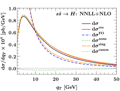
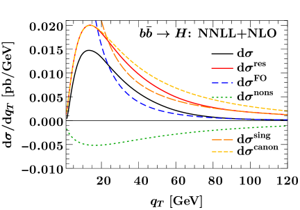
Figure -1197: Different contributions entering the matching procedure for $s\bar{s}\to H$ (left) and $b\bar{b}\to H$ (right) at NNLL$+$NLO. The final matched result $\mathrm{d}\sigma$ (solid black) is the sum of the nominal resummed $\mathrm{d}\sigma^{\mathrm{res}}$ (solid red) and the nonsingular $\mathrm{d}\sigma^{\mathrm{nons}}$ (dashed green). The fixed-order result $\mathrm{d}\sigma^{\mathrm{FO}}$ (dashed blue) is the sum of the fixed-order singular $\mathrm{d}\sigma^{\mathrm{sing}}$ (long-dashed orange) and $\mathrm{d}\sigma^{\mathrm{nons}}$ (dashed green). Here, the canonically resummed result is denoted as $\mathrm{d}\sigma^{\mathrm{canon}}$ (short-dashed yellow). The nominal resummed $\mathrm{d}\sigma^{\mathrm{res}}$ transitions from $\mathrm{d}\sigma^{\mathrm{canon}}$ at small $q_{T}$ to $\mathrm{d}\sigma^{\mathrm{sing}}$ at large $q_{T}$.

This difference between the channels can be understood from the very different size of the quark PDFs involved. At lowest order, the nonsingular receives contributions from two different flavour channels, namely $q\bar{q}\to Hg$ and $gq\to Hq$ (which includes $g\bar{q}\to H\bar{q}$ for the sake of this discussion). In Drell-Yan, these two channels have opposite sign and similar size (see e.g. ref. [97]), and thus partially cancel each other, leading to the relatively small nonsingular corrections typical for that process. The same also happens for $s\bar{s}\to H$. For $b\bar{b}\to H$, however, the very small $b$-quark PDF suppresses the $b\bar{b}$-induced contributions. This has two effects leading to the observed behaviour: first, the nonsingular is dominated by the gluon-induced channels leading to smaller cancellations. This is compounded by the fact that the leading (NLL) contributions in the resummed are also $b\bar{b}$ induced and numerically suppressed. Both of these effects numerically enhance the nonsingular. The second effect furthermore causes a larger difference between (canonically) resummed and fixed-order singular. From this discussion one would expect the $c\bar{c}\to H$ process (not shown in figure -1197) to exhibit behaviour intermediate between $s\bar{s}\to H$ and $b\bar{b}\to H$, which is indeed the case.

The stronger sensitivity to the (ultimately arbitrary) choice of transition points in $b\bar{b}\to H$ requires us to take greater care in choosing the transition points and in estimating the associated matching uncertainty. Usually, the start and endpoints of the transition, $x_{1}$ and $x_{3}$ (see section 2.3) are chosen based on examining the relative sizes of the singular and nonsingular pieces as a function of $q_{T}$, as shown in figure -1196 for $s\bar{s}\to H$ (left) and $b\bar{b}\to H$ (right). The rather different behaviour of the channels is seen again here. The $s\bar{s}\to H$ channel again looks very similar to Drell-Yan, with the nonsingular becoming important only at relatively large $q_{T}/m_{H}\gtrsim 0.8$, such that a typical choice for the transition points would be $x_{1}=0.3$, $x_{3}=0.9$, $x_{2}=(x_{1}+x_{3})/2=0.6$ [64, 45]. In contrast, for $b\bar{b}\to H$ the nonsingular becomes important much earlier. Based on this plot, one might take sensible central values of $x_{1}=0.2$, $x_{3}=0.7$, and $x_{2}=(x_{1}+x_{3})/2=0.45$.

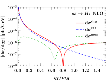
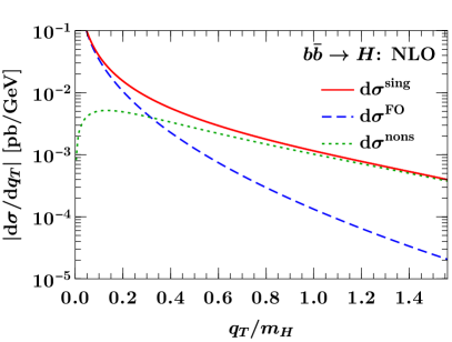
Figure -1196: Singular (solid red), full (dashed blue), and nonsingular (dotted green) contributions at fixed $\mathcal{O}(\alpha_{s})$ as a function of $q_{T}/m_{H}$ for $s\bar{s}\to H$ (left) and $b\bar{b}\to H$ (right).

The matching uncertainty $\Delta_{\mathrm{match}}$ is related to the ambiguity in these choices. The standard method to estimate it is to vary $x_{1}$ and $x_{3}$, typically by $\pm 0.1$, with $x_{2}$ given by $(x_{1}+x_{3})/2$ for any given variation. The resulting variations for $b\bar{b}\to H$ are shown in figure -1195. We first note that this standard method leads by construction to a one-sided uncertainty above the central $x_{3}$ and below the central $x_{1}$, because varying $x_{3}$ up or $x_{1}$ down can only change the cross section in one direction. In practical applications, e.g. when propagating the $x_{1,3}$ variations in a fit, this is a rather undesirable feature. Furthermore, varying $x_{1}$ and $x_{3}$ up (long-dashed green) produces an unreasonably large uncertainty. The reason for this large variation, as evident from the left plot, is precisely due to the rather large difference between the canonically resummed and fixed-order results already discussed, between which the transition must interpolate.

We therefore adopt a somewhat different approach to estimate the matching uncertainty. We first fix $x_{1}$ to its lowest and $x_{3}$ to its highest reasonable value, e.g. to their respective minimum and maximum values one would consider in the previous approach (which are $x_{1}=0.1$ and $x_{3}=0.8$ in our example). We then vary the point $x_{2}$ to estimate the matching uncertainty. Conceptually, this effectively varies whether the transition happens earlier or later within the maximal window in which the transition should occur. Here, we take $x_{2}=(x_{1}+x_{3})/2=0.45$ as our central value and vary it within the range $[0.2,0.6]$. Note that the size of this range is twice that of the $x_{1}$ and $x_{3}$ variations, so the total amount of variation is preserved. The resulting variations are shown in figure -1194.

We begin by observing that this method avoids the undesired one-sided uncertainties, although the uncertainty is still somewhat asymmetric at any given $q_{T}$. This is practically unavoidable, since it is inherent to the nature of the matching uncertainty. We can, however, choose the $x_{2}$ range of variation such that the maximum up and down variations in the cross section are of similar size, which is why we vary it further down than up. Furthermore, the $x_{2}$ variation yields a much more reasonable size for the matching uncertainty. Finally, this method has the added benefit that the matching uncertainty is now parameterized by a single variable. This makes it much easier to propagate in practice, as it avoids having to take envelopes of different parameter variations.

For our final numerical results, the matching uncertainty $\Delta_{\mathrm{match}}$ is still obtained as the maximum of the absolute impact of varying $x_{2}$ down to $0.2$ and up to $0.6$. However, this is now just for ease of presentation and not a requirement. Since $s\bar{s}\to H$ and $c\bar{c}\to H$ are less sensitive to the precise transition, we will use the same central values and $x_{2}$ variations for simplicity.

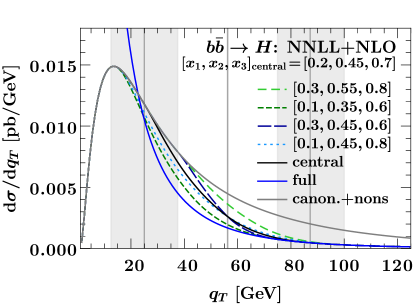
Figure -1195: Standard variation of the transition points $x_{1}$ and $x_{3}$ for $b\bar{b}\to H$ at NNLL$+$NLO. The absolute variation in the spectrum is shown on the left, and the relative variation with respect to the central result is shown on the right. The vertical lines indicate the central values $[x_{1},x_{2},x_{3}]=[0.2,0.45,0.7]$, and the grey bands the variations of $x_{1}$ and $x_{3}$ by $\pm 0.1$, where always $x_{2}=(x_{1}+x_{3})/2$.

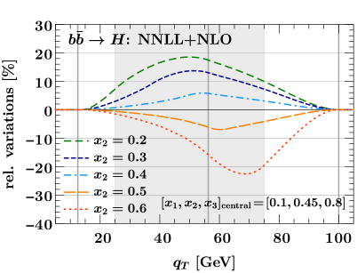
Figure -1194: New variation of the transition point $x_{2}$ for $b\bar{b}\to H$ at NNLL$+$NLO. The absolute variation in the spectrum is shown on the left, and the relative variation with respect to the central result is shown on the right. The vertical lines indicate the central values $[x_{1},x_{2},x_{3}]=[0.1,0.45,0.8]$, where $x_{1}$ and $x_{3}$ are fixed to their respective minimum and maximum values used in figure -1195. The grey band shows the variation in $x_{2}$ from $0.2$ to $0.6$.

3.3 Decorrelation of singular and nonsingular contributions

As discussed in section 3.1, we wish to construct an approximate result for $\mathrm{d}\sigma^{\mathrm{FO}}$ at NNLO₁, which we can consistently match to $\mathrm{d}\sigma^{\mathrm{res}}$ at N³LL^′. As discussed in section 2.3, this requires that the NNLO₁ cross section contains the correct singular terms $\mathrm{d}\sigma^{\mathrm{sing}}$, which are part of the N³LL^′ result. We must therefore approximate the remaining nonsingular part of the full NNLO₁. However, as also discussed in section 2.3, at large $q_{T}$ there is a strong cancellation between singular and nonsingular, which means the two pieces are strongly correlated and only the full fixed-order result is meaningful there. Hence, at large $q_{T}$ we should do the opposite and approximate the full result, considering the nonsingular as a derived quantity given by the difference of full and singular. To satisfy these competing requirements, we introduce a general method to decorrelate the singular and nonsingular contributions, which we will then use in the next subsection to construct the actual approximation.

The basic idea behind the decorrelation of the singular and nonsingular contributions at large $q_{T}$ involves shifting a correlated piece between the two [52],

$$\mathrm{d}\sigma^{\mathrm{FO}}(q_{T}) =\mathrm{d}\sigma^{\mathrm{sing}}(q_{T})+\mathrm{d}\sigma^{\mathrm{nons}}(q_{T})$$

$$=\underbrace{\mathrm{d}\sigma^{\mathrm{sing}}(q_{T})+\mathrm{d}\sigma^{\mathrm{corr}}(q_{T})}_{\mathrm{d}\tilde{\sigma}^{\mathrm{sing}}}+\underbrace{\mathrm{d}\sigma^{\mathrm{nons}}(q_{T})-\mathrm{d}\sigma^{\mathrm{corr}}(q_{T})}_{\mathrm{d}\tilde{\sigma}^{\mathrm{nons}}}\equiv\mathrm{d}\tilde{\sigma}^{\mathrm{sing}}(q_{T})+\mathrm{d}\tilde{\sigma}^{\mathrm{nons}}(q_{T})\,,$$ (3.2)

where here and below we use the notation $\mathrm{d}\sigma(q_{T})\equiv\mathrm{d}\sigma/\mathrm{d}q_{T}$ to make the $q_{T}$ dependence explicit. We call $\mathrm{d}\tilde{\sigma}^{\mathrm{sing}}(q_{T})$ and $\mathrm{d}\tilde{\sigma}^{\mathrm{nons}}(q_{T})$ the decorrelated singular and nonsingular contributions. The correlated piece $\mathrm{d}\sigma^{\mathrm{corr}}(q_{T})$ is as of yet unspecified.

To achieve the desired decorrelation, we require the decorrelated nonsingular to become equal to the full fixed-order result toward large $q_{T}$, and as a consequence the decorrelated singular to vanish,

$$\mathrm{d}\tilde{\sigma}^{\mathrm{nons}}(q_{T}\to m_{H})\to\mathrm{d}\sigma^{\mathrm{FO}}(q_{T})\,,\qquad\mathrm{d}\tilde{\sigma}^{\mathrm{sing}}(q_{T}\to m_{H})\to 0\,.$$ (3.3)

This guarantees that no cancellations occur between them. At the same time, the decorrelated nonsingular must remain power suppressed for $q_{T}\ll m_{H}$, such that the decorrelated singular still contains all singular terms,

$$\frac{\mathrm{d}\tilde{\sigma}^{\mathrm{nons}}(q_{T})}{\mathrm{d}\sigma^{\mathrm{sing}}(q_{T})}\sim\mathcal{O}\Bigl{(}\frac{q_{T}^{2}}{m_{H}^{2}}\Bigr{)}\,,\qquad\mathrm{d}\tilde{\sigma}^{\mathrm{sing}}(q_{T})=\mathrm{d}\sigma^{\mathrm{sing}}(q_{T})\biggl{[}1+\mathcal{O}\Bigl{(}\frac{q_{T}^{2}}{m_{H}^{2}}\Bigr{)}\biggr{]}\,.$$ (3.4)

These two conditions are equivalent to the following two conditions on $\mathrm{d}\sigma^{\mathrm{corr}}(q_{T})$,

$$\mathrm{d}\sigma^{\mathrm{corr}}(q_{T}\to m_{H})\to-\mathrm{d}\sigma^{\mathrm{sing}}(q_{T})\,,\qquad\frac{\mathrm{d}\sigma^{\mathrm{corr}}(q_{T})}{\mathrm{d}\sigma^{\mathrm{sing}}(q_{T})}\sim\mathcal{O}\Bigl{(}\frac{q_{T}^{2}}{m_{H}^{2}}\Bigr{)}\,.$$ (3.5)

The easiest way to satisfy these conditions might be simply to take $\mathrm{d}\sigma^{\mathrm{corr}}(q_{T})$ to be a constant, $\mathrm{d}\sigma^{\mathrm{corr}}(q_{T})=-\mathrm{d}\sigma^{\mathrm{sing}}(m_{H})$. This is equivalent to what was used in ref. [52], where the analogous decorrelation was used in a similar context. In that particular case, the phase space was strictly bounded to the equivalent of $q_{T}\leq m_{H}$. In contrast, this is no longer possible in our case: the phase space does not have such a strict boundary, and the decorrelation condition in eq. (3.3) must hold not only at the single point $q_{T}=m_{H}$ but for any $q_{T}\gtrsim m_{H}$. In other words, we require not only that $\mathrm{d}\tilde{\sigma}^{\mathrm{sing}}(q_{T})$ crosses through $0$ at $q_{T}=m_{H}$, but also that it remains zero for any larger $q_{T}$. Furthermore, a constant value for $\mathrm{d}\sigma^{\mathrm{corr}}(q_{T})$ only corresponds to a linear power suppression of $\mathcal{O}(q_{T}/m_{H})$. To obtain the correct quadratic power suppression of $\mathcal{O}(q_{T}^{2}/m_{H}^{2})$, the correct extension of ref. [52] to our case is to take $\mathrm{d}\sigma^{\mathrm{corr}}/\mathrm{d}q_{T}^{2}$ to be a constant.

To achieve this, let us denote $s(q_{T})\equiv\mathrm{d}\sigma/\mathrm{d}q_{T}^{2}$ and choose $\mathrm{d}\sigma^{\mathrm{corr}}(q_{T})$ more generally such that

$$s^{\mathrm{corr}}(q_{T}) =-s^{\mathrm{sing}}(q_{T})\quad \text{for}\quad q_{T}\sim m_{H}\,,$$

$$s^{\mathrm{corr}}(q_{T}) =-s^{\mathrm{sing}}(\kappa m_{H})=\text{const.}\quad \text{for}\quad q_{T}\ll m_{H}\,.$$ (3.6)

That is, $s^{\mathrm{corr}}(q_{T})$ is given by $-s^{\mathrm{sing}}(q_{T})$ at large $q_{T}$ and freezes to a constant $-s^{\mathrm{sing}}(\kappa m_{H})$ at small $q_{T}$, where $\kappa\sim 1$ is a constant of our choice. To make this a smooth transition, we can reuse our profile functions and take

$$s^{\mathrm{corr}}(q_{T})=-s^{\mathrm{sing}}[\tilde{q}_{T}(q_{T})]\,,$$ (3.7)

where $\tilde{q}_{T}(q_{T})$ is a function of $q_{T}$ that transitions from $\kappa m_{H}$ to $q_{T}$,

$$\tilde{q}_{T}(q_{T})=\kappa\,m_{H}\,g_{\mathrm{run}}(q_{T}/m_{H})+q_{T}[1-g_{\mathrm{run}}(q_{T}/m_{H})]\,,$$ (3.8)

and $g_{\mathrm{run}}(q_{T})$ is defined as in eq. (2.13). For simplicity, we will use the same transition points $[0.1,0.45,0.8]$ which we use for turning off the resummation (see section 2.3). Using eq. (3.7), we arrive at our final choice for $\mathrm{d}\sigma^{\mathrm{corr}}(q_{T})$,

$$\mathrm{d}\sigma^{\mathrm{corr}}(q_{T})=-2q_{T}\,s^{\mathrm{sing}}[\tilde{q}_{T}(q_{T})]=-\frac{q_{T}}{\tilde{q}_{T}(q_{T})}\,\mathrm{d}\sigma^{\mathrm{sing}}[\tilde{q}_{T}(q_{T})]\,.$$ (3.9)

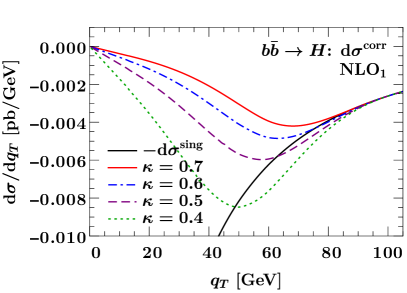
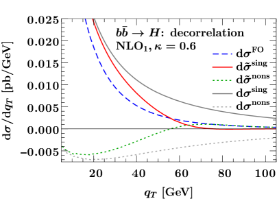
Figure -1193: Decorrelation of singular and nonsingular at NLO₁. Left: Correlated contribution for different choices of $\kappa$ (coloured lines) and its large-$q_{T}$ asymptotic value $-\mathrm{d}\sigma^{\mathrm{sing}}$ (black). Right: Decorrelated singular (solid red), full, (dashed blue), and decorrelated nonsingular (dotted green) for $\kappa=0.6$ at fixed NLO₁. The original, correlated singular and nonsingular are shown by the dotted and solid grey lines.

In figure -1193, we study the decorrelation procedure at NLO₁, where the fixed-order result is fully known. The left panel of the figure shows the correlated piece $\mathrm{d}\sigma^{\mathrm{corr}}(q_{T})$ for different choices of $\kappa$ alongside $-\mathrm{d}\sigma^{\mathrm{sing}}(q_{T})$. For $q_{T}\geq x_{3}m_{H}=100\,\mathrm{GeV}$, $\mathrm{d}\sigma^{\mathrm{corr}}(q_{T})$ exactly equals $-\mathrm{d}\sigma^{\mathrm{sing}}(q_{T})$, while going to lower $q_{T}$ it starts to deviate and eventually turn around and vanish linearly for $q_{T}\to 0$ as required by eq. (3.9). The correlated contribution itself depends strongly on the choice of $\kappa$, which determines where it effectively freezes out and turns around toward $0$. Note also that by construction this dependence cancels exactly, such that the full result at this order is independent of $\kappa$. The actual choice of $\kappa$ could in principle influence our NNLO₁ approximation, but essentially does not do so, as we shall see in the following subsection.

The right panel of figure -1193 shows both the original, correlated singular (solid grey) and nonsingular (dotted grey) as well as the decorrelated singular (solid red) and nonsingular (dotted green) for $\kappa=0.6$. Since they each sum to the fixed-order result (dashed blue), the correlated terms clearly exhibit a large cancellation for large $q_{T}\sim m_{H}$. In contrast, the decorrelated singular goes to zero for $q_{T}\sim m_{H}$, while the decorrelated nonsingular (dotted green) becomes equal to the full fixed order. This confirms that the decorrelation works as expected, and that $\mathrm{d}\tilde{\sigma}^{\mathrm{nons}}$ and $\mathrm{d}\tilde{\sigma}^{\mathrm{sing}}$ no longer exhibit strong cancellations. We will therefore use $\kappa=0.6$ for $b\bar{b}\to H$. Since the strong cancellations between singular and nonsingular occur successively later for $c\bar{c}\to H$ and $s\bar{s}\to H$, as we saw in section 3.2, we will use higher values $\kappa=0.7$ for $c\bar{c}\to H$ and $\kappa=0.8$ for $s\bar{s}\to H$.

3.4 aNNLO₁

Using the decorrelation method explained in the previous section, we are now in a position to construct an approximate NNLO₁ result as

$$\mathrm{d}\sigma^{\mathrm{FO}}(q_{T})=\mathrm{d}\tilde{\sigma}^{\mathrm{sing}}(q_{T})+\mathrm{d}\tilde{\sigma}^{\mathrm{nons}}(q_{T})=\mathrm{d}\sigma^{\mathrm{sing}}(q_{T})+\mathrm{d}\sigma^{\mathrm{corr}}(q_{T};\kappa)+\mathrm{d}\tilde{\sigma}^{\mathrm{nons}}(q_{T};\kappa)\,,$$ (3.10)

where we made the dependence on $\kappa$ in the last two terms explicit. We now need to approximate the unknown $\mathcal{O}(\alpha_{s}^{3})$ contribution of $\mathrm{d}\tilde{\sigma}^{\mathrm{nons}}(q_{T})$. To do so, we decompose $\mathrm{d}\tilde{\sigma}^{\mathrm{nons}}$ at the fixed scale $\mu_{R}=\mu_{F}=m_{H}$ in terms of perturbative coefficients $\tilde{c}_{i}(q_{T})$,

$$\mathrm{d}\tilde{\sigma}^{\mathrm{nons}}(q_{T})=|y_{b}(m_{H})|^{2}\Bigl{[}{\alpha_{s}(m_{H})}\,\tilde{c}_{1}(q_{T})+\alpha_{s}^{2}(m_{H})\,\tilde{c}_{2}(q_{T})+\alpha_{s}^{3}(m_{H})\,\tilde{c}_{3}(q_{T})\Bigr{]}\,,$$ (3.11)

where $\tilde{c}_{1}(q_{T})$ and $\tilde{c}_{2}(q_{T})$ are known, and our goal is to approximate $\tilde{c}_{3}(q_{T})$. To get the correct power of logarithms for $\tilde{c}_{3}(q_{T})$, we perform a Padé-like approximation

$$\tilde{c}_{3}^{\rm approx}(q_{T})=K\,\frac{[\tilde{c}_{2}(q_{T})]^{2}}{\tilde{c}_{1}(q_{T})}\,,$$ (3.12)

where we use the constant factor $K$ to rescale this result such that its overall size agrees with ref. [33]. When using this approximation in eq. (3.10), we refer to the result as aNNLO₁.

To determine an appropriate value for $K$, we consider the ratio of our approximate $\mathcal{O}(\alpha_{s}^{3})$ coefficient to the exact result shown on the right in figure -1192. The exact $\mathcal{O}(\alpha_{s}^{3})$ coefficient is obtained by subtracting NNLO${}_{1}-$NLO₁, where we can read off the ratio NNLO${}_{1}/$NLO₁ from the results shown in ref. [33]. As already mentioned, ref. [33] uses a cut on the leading jet $p_{T}\geq 30\,\mathrm{GeV}$, so we can only use their results for $q_{T}\geq 60\,\mathrm{GeV}$. For this purpose we use the same inputs as ref. [33], i.e., $\mu_{F}=m_{H}/2$ and the CT14nnlo PDF set. To extract a value for $K$, we perform a simple $\chi^{2}$ fit to this ratio as a function of $K$, requiring that the ratio is unity. Since the kinematic region we are interested in is $q_{T}\lesssim m_{H}$, we use the first four points for $q_{T}\in[60,140]\,\mathrm{GeV}$. Note that in this region the ratio is well approximated by a constant, which shows that the approximation in eq. (3.12) captures the $q_{T}$ dependence well. We find $K=0.75$, which we will use as our default value. We refrain from including an uncertainty on $K$, since it would be negligible compared to the nominal perturbative uncertainties.

The left panel of figure -1192 shows the ratio NNLO${}_{1}/$NLO₁ for the exact NNLO₁ result from ref. [33] (green) as well as for our approximate aNNLO₁ for $K=1$ (blue) and our default $K=0.75$ (red). The uncertainties correspond to varying $\mu_{R}$ and $\mu_{F}$ by a factor of 2. For our default $K$, we find very good agreement in the region of interest $q_{T}\lesssim m_{H}$ between our approximation and the exact results.

We then use the same value of $K$ also at lower values of $q_{T}$ as well as for the $s\bar{s}\to H$ and $c\bar{c}\to H$ channels and our default PDF set. That is, we effectively use our approximation to extrapolate the exact results from ref. [33] to lower $q_{T}$ and the other channels and PDF.

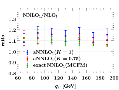
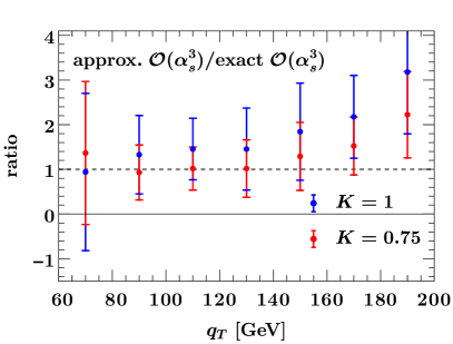
Figure -1192: Comparison of the exact NNLO₁ results from ref. [33] at large $q_{T}$ to our approximation. Left: Ratio of NNLO${}_{1}/$NLO₁ for the exact result (green) and the approximate result with $K=1$ (blue) and $K=0.7$ (red). Right: Ratio of the approximate and exact $\mathcal{O}(\alpha_{s}^{3})$ contribution for $K=1$ (blue) and $K=0.7$ (red). The uncertainties in all cases correspond to the scale variations.

The coefficients $\tilde{c}_{i}(q_{T})$ depend on the choice of $\kappa$. For the exact coefficients, the $\kappa$ dependence exactly cancels between the last two terms in eq. (3.10). However, when using the approximate $\tilde{c}_{3}^{\rm approx}(q_{T})$, the $\kappa$ dependence will no longer cancel exactly. The residual $\kappa$ dependence of the aNNLO₁ result is shown in the left panel of figure -1191. Happily, we find that the approximate result is practically independent of the value of $\kappa$. In the right panel of figure -1191, we illustrate the decomposition of the approximated full result for our default choice $\kappa=0.6$ into the decorrelated singular and nonsingular pieces.

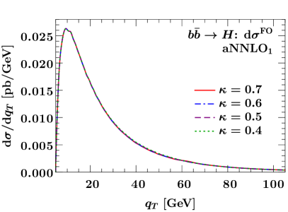
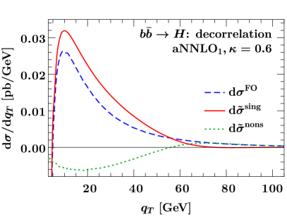
Figure -1191: Decorrelation at aNNLO₁. Left: The resulting full fixed-order order cross section for different values of $\kappa$. Right: Decorrelated singular (solid red), full (dashed blue), and decorrelated nonsingular (dotted green) for $\kappa=0.6$.

To obtain the correct scale dependence for the approximated result, we re-expand $\alpha_{s}(m_{H})$ and $y_{b}(m_{H})$ in terms of $\alpha_{s}(\mu_{R})$, which yields

$$\frac{\mathrm{d}\tilde{\sigma}^{\mathrm{nons}}}{\mathrm{d}q_{T}} =|y_{b}(\mu_{R})|^{2}\biggl{\{}\alpha_{s}(\mu_{R})\,\tilde{c}_{1}(q_{T})+\alpha_{s}^{2}(\mu_{R})\biggl{[}\tilde{c}_{2}(q_{T})+\frac{\tilde{c}_{1}}{2\pi}(\beta_{0}-\gamma_{0})\ln\frac{\mu_{R}}{m_{H}}\biggr{]}$$

$$\quad+\alpha_{s}^{3}(\mu_{R})\biggl{[}\tilde{c}_{3}(q_{T})+\Bigl{[}\frac{\tilde{c}_{1}(q_{T})}{8\pi^{2}}(\beta_{1}-\gamma_{1})+\frac{\tilde{c}_{2}(q_{T})}{2\pi}(2\beta_{0}-\gamma_{0})\Bigr{]}\ln\frac{\mu_{R}}{m_{H}}$$

$$\qquad\qquad\qquad+\frac{\tilde{c}_{1}(q_{T})}{8\pi^{2}}(2\beta_{0}^{2}-3\beta_{0}\gamma_{0}+\gamma_{0}^{2})\ln^{2}\frac{\mu_{R}}{m_{H}}\biggr{]}\biggr{\}}\,,$$ (3.13)

where $\beta_{n}$ and $\gamma_{n}$ are the relevant coefficients of the QCD beta function and the Yukawa anomalous dimension,

$$\beta_{0} =\frac{11}{3}C_{A}-\frac{4}{3}T_{F}n_{f}\,,\qquad \beta_{1} =\frac{34}{3}C_{A}-\left(\frac{20}{3}C_{A}+4C_{F}\right)T_{F}n_{f}\,,$$

$$\gamma_{0} =-6C_{F}\,,\qquad \gamma_{1} =-2C_{F}\left(\frac{3}{2}C_{F}+\frac{97}{6}C_{A}-\frac{10}{3}T_{F}n_{f}\right)\,.$$ (3.14)

The $\mu_{R}$ dependence in the approximated result is therefore exact, and we are able to vary $\mu_{R}$ without further approximation.

For the $\mu_{F}$ dependence, for simplicity we perform the approximation for $\tilde{c}_{3}(q_{T})$ in eq. (3.12) in terms of $\tilde{c}_{1}(q_{T})$ and $\tilde{c}_{2}(q_{T})$ at any given $\mu_{F}$, using the same rescaling factor $K$ as for the central $\mu_{F}$ choice. This means we will only have an approximate $\mu_{F}$ dependence at $\mathcal{O}(\alpha_{s}^{3})$ that only approximately cancels up to higher $\mathcal{O}(\alpha_{s}^{4})$ terms. This will lead to slightly larger $\mu_{F}$ variations compared to the exact $\mathcal{O}(\alpha_{s}^{3})$ $\mu_{F}$ dependence, which we can simply consider as an additional uncertainty due to the approximation.

4 Results

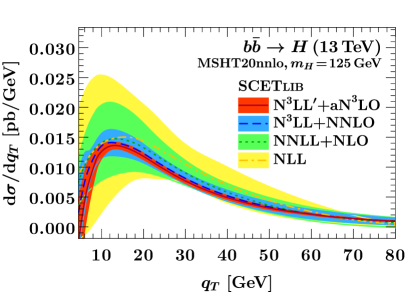
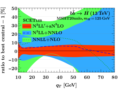
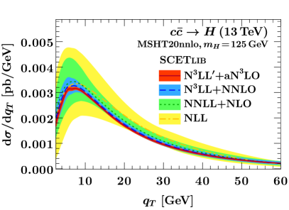
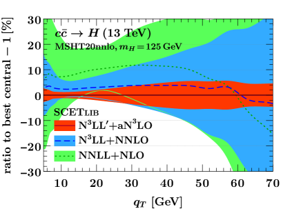
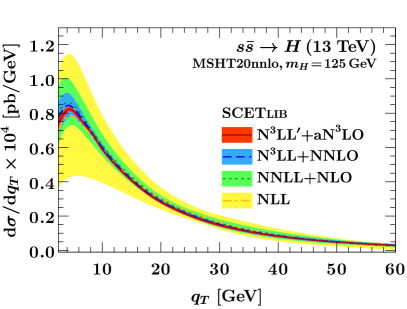
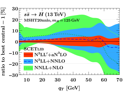
Figure -1190: Resummed $q_{T}$ spectrum up to N³LL${}^{\prime}+$aN³LO for $b\bar{b}\to H$ (top row), $c\bar{c}\to H$ (middle row), and $s\bar{s}\to H$ (bottom row). The results for the spectrum are shown on the left. The results normalized relative to the best central value at N³LL${}^{\prime}+$aN³LO are shown on the right.

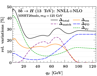
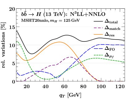
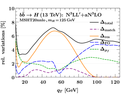
Figure -1189: Breakdown of the perturbative uncertainties into its different contributions for $b\bar{b}\to H$ at NNLL$+$NLO (top), N³LL$+$NNLO (bottom left), and N³LL${}^{\prime}+$aN³LO (bottom right). Note the different scales on the vertical axes for each plot.

In this section, we present our numerical result for the $q\bar{q}\to H$ $q_{T}$ spectrum. We use $E_{\mathrm{cm}}=13\,\mathrm{TeV}$, $m_{H}=125\,\mathrm{GeV}$, and the MSHT20nnlo PDF set [98] with $\alpha_{s}(m_{Z})=0.118$. We assess the impact of changing the PDF set to MSHT20an3lo [99] in appendix C. For the Yukawa coupling we evolve $\overline{m}_{q}(\mu_{q})$ to $\mu_{\mathrm{FO}}$ where $\mu_{b,c}=\overline{m}_{b,c}$ for the bottom and charm quarks and $\mu_{s}=2\,\mathrm{GeV}$ for the strange quark. The input $\overline{\mbox{MS}}$ quark masses are $\overline{m}_{b}(\overline{m}_{b})=4.18\,\mathrm{GeV}$, $\overline{m}_{c}(\overline{m}_{c})=1.27\,\mathrm{GeV}$, and $\overline{m}_{s}(2\,\mathrm{GeV})=93.4\,\mathrm{MeV}$ [100], and we use $v=246.22\,\mathrm{GeV}$ for the Higgs vev to convert the masses into Yukawa couplings. Our scale choices are described in section 2.3. All our numerical results for the resummed and fixed-order singular contributions are obtained with SCETlib [88]. The full fixed-order results are obtained as discussed in sections 3.1 and 3.4. For the aNNLO₁ result we use the parameters $\kappa=0.6$ and $K=0.7$.

In figure -1190, we show the resummed $q_{T}$ spectrum for $b\bar{b}\to H$ (top), $c\bar{c}\to H$ (middle) and $s\bar{s}\to H$ (bottom) at different resummation orders up to the highest N³LL${}^{\prime}+$aN³LO. The bands show the perturbative uncertainty estimate as discussed in section 2.4. We observe excellent perturbative convergence for all channels, with reduced uncertainties at each higher order. The perturbative uncertainties increase in general from $s\bar{s}\to H$, to $c\bar{c}\to H$, to $b\bar{b}\to H$. Comparing the ratio plots for $s\bar{s}\to H$ and $b\bar{b}\to H$ it is evident that the relative uncertainties for $b\bar{b}\to H$ at a given order are of similar size as those for $s\bar{s}\to H$ at one lower order. As already mentioned in section 3.2, the main difference between the channels is the relative size of the PDF luminosities. Since for $b\bar{b}\to H$, the $b\bar{b}$ Born channel is numerically suppressed by the small $b$-quark PDFs, the gluon-induced PDF channels which start at one higher order play a much more prominent role. This explains the observed pattern of uncertainties for the different cases.

Our default choice for the PDF scale $\mu_{f}$ corresponds to taking $\mu_{F}=m_{H}$ in the fixed-order limit. Fixed-order predictions for $b\bar{b}\to H$ traditionally use a lower scale of $\mu_{F}=m_{H}/2$ or $\mu_{F}=m_{H}/4$, so one might wonder whether the uncertainties for $b\bar{b}\to H$ might be reduced by choosing a lower central value for $\mu_{F}$. In appendix C we provide analogous resummed results for these lower $\mu_{F}$ choices, which show that in fact the opposite is the case: by lowering $\mu_{F}$, the perturbative convergence for the resummed $q_{T}$ spectrum gets noticeably worse, justifying our default choice for $\mu_{F}$.

A detailed breakdown of the uncertainty estimate for $b\bar{b}\to H$ is shown in figure -1189. The $\Delta_{\mu_{f}}$ uncertainty (short-dashed green) dominates up to $q_{T}\lesssim 20\,\mathrm{GeV}$ before tending to a constant for $q_{T}\gtrsim 80\,\mathrm{GeV}$. At NNLL$+$NLO the matching uncertainty $\Delta_{\mathrm{match}}$ (long-dashed purple) is largest for $30\,\mathrm{GeV}\lesssim q_{T}\lesssim 80\,\mathrm{GeV}$ and vanishes outside of the transition region as it should. At higher orders, the resummation uncertainty $\Delta_{\mathrm{res}}$ (solid orange) dominates in this region before going to zero as the resummation is turned off toward large $q_{T}$. As one might expect, at the same time the fixed-order uncertainty $\Delta_{\mathrm{FO}}$ (dashed blue) increases and becomes the dominant uncertainty in the fixed-order region.

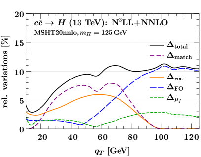
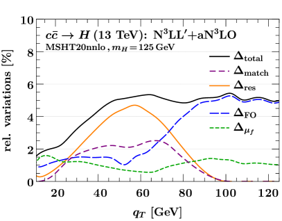
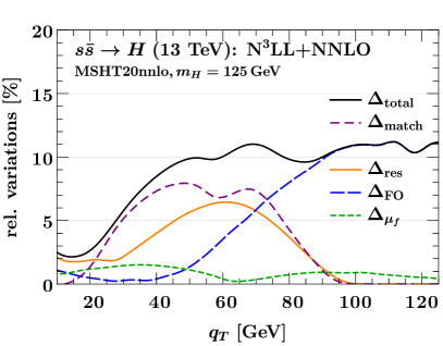
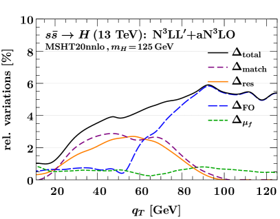
Figure -1188: Breakdown of the perturbative uncertainties into its different contributions for $c\bar{c}\to H$ (left) and $s\bar{s}\to H$ (right) at N³LL$+$NNLO (top) and N³LL${}^{\prime}+$aN³LO (bottom).

In figure -1188, we show the impact of the individual uncertainties for $c\bar{c}\to H$ and $s\bar{s}\to H$. In general, they display a behaviour very similar to $b\bar{b}\to H$. The main difference between the processes is the size of the resummation and the matching uncertainty. The matching uncertainty is slightly smaller for $b\bar{b}\to H$; this is to be expected, since we chose our transition points in section 3.2 for this specific case. On the other hand, $\Delta_{\mathrm{res}}$ is smaller for $c\bar{c}\to H$ and $s\bar{s}\to H$. The total uncertainty for $s\bar{s}\to H$ is therefore dominated by $\Delta_{\mathrm{match}}$ for $30\,\mathrm{GeV}\lesssim q_{T}\lesssim 70\,\mathrm{GeV}$. For $c\bar{c}\to H$, $\Delta_{\mathrm{match}}$ has the largest impact at N³LL$+$NNLO whereas at N³LL${}^{\prime}+$aN³LO $\Delta_{\mathrm{res}}$ contributes the most. The fixed-order uncertainty starts to dominate the total uncertainty slightly earlier than for $b\bar{b}\to H$ as the other contributions are in general smaller.

In figure -1187, we compare the normalized $q_{T}$ spectra for $s\bar{s}\to H$ (red), $c\bar{c}\to H$ (blue), and $b\bar{b}\to H$ (green). The left panel shows the spectra at NNLL$+$NLO, where one can already see that the spectra of the channels exhibit different shapes. At this order however the uncertainties largely overlap in the peak region. The right panel shows the spectra at N³LL${}^{\prime}+$aN³LO. Here, the uncertainties are significantly smaller and we can clearly distinguish the channels by their different shapes in $q_{T}$. Our predictions could therefore be used to improve the determination of quark Yukawa coupling from the shape of the measured Higgs $q_{T}$ spectrum – such an analysis has already been performed in refs. [38, 39], using measurements in the $H\to ZZ^{*}\to 4\ell$ and $H\to\gamma\gamma$ decay channels.

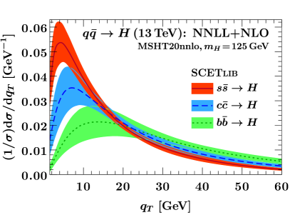
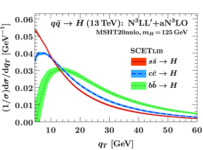
Figure -1187: Comparison of the normalized $q_{T}$ spectrum for $s\bar{s}\to H$, $c\bar{c}\to H$, and $b\bar{b}\to H$ at NNLL$+$NLO (left) and N³LL${}^{\prime}+$aN³LO (right).

5 Conclusions

In this work, we have studied the transverse momentum spectrum of the Higgs boson produced in heavy quark annihilation, $q\bar{q}\to H$ with $q=s,c,b$. This is an interesting process, as it has the potential to constrain the Yukawa couplings of charm, bottom, and possibly strange quarks. We have used soft-collinear effective theory to resum large logarithms of $q_{T}/m_{H}$ up to N³LL^′ order and matched these results to fixed-order calculations. For $b\bar{b}\to H$ and to a lesser extent $c\bar{c}\to H$, the large size of the nonsingular terms requires extra care in the matching procedure and the estimation of matching uncertainties. Accordingly, we introduced some refinements to the standard method when using profile-scale variations, which could also be useful in other contexts. It consists of fixing the extreme profile function transition points and varying instead the central point over a wider range. This leads to an uncertainty estimate without one-sided uncertainties, and which in our case avoids being overly conservative.

We have constructed an approximation of the $q_{T}$ spectrum at fixed $\mathcal{O}(\alpha_{s}^{3})$, which we have used to extrapolate from existing NNLO₁ results for $b\bar{b}\to H+j$ for $q_{T}\geq 60\,\mathrm{GeV}$ to smaller $q_{T}$ and other flavour channels. This is based on introducing a decorrelation procedure to ensure the correct cancellation between singular and nonsingular terms at scales $q_{T}\sim m_{H}$, and then approximating the $\mathcal{O}(\alpha_{s}^{3})$ nonsingular piece. This allows us to achieve a final accuracy of N³LL^′+aN³LO for the $q_{T}$ spectrum. Our results display good convergence properties from order to order, and constitute the highest available accuracy for these processes. As we have seen in figure -1187, at the highest available order the uncertainties are significantly reduced, such that the different flavour channels are clearly distinguishable by their different shapes in $q_{T}$. Our predictions could therefore be used to improve the determination of Higgs Yukawa couplings from the Higgs $q_{T}$ spectrum as carried out in refs. [38, 39].

Our treatment of the $q\bar{q}\to H$ process in this work has neglected finite quark-mass effects, which are relevant for $q_{T}\sim m_{q}$ and are thus an important consideration especially for $b\bar{b}\to H$. The inclusion of these terms in the resummation formalism has been derived for the Drell-Yan process in ref. [51], and the extension to our case would be relatively straightforward. It would also be interesting to investigate in more detail the impact of the resummation of time-like logarithms in the $q\bar{q}H$ hard function on the resummed $q_{T}$ spectrum, as it has been shown to have a nontrivial impact on the inclusive $b\bar{b}\to H$ cross section [65]. Finally, we have only considered the $q_{T}$ spectrum for inclusive Higgs production here. Experimentally required cuts on the Higgs decay products induce fiducial power corrections [101, 64], which were found to be important in case of $gg\to H$ production [40]. It would thus be interesting to investigate their importance also in case of $q\bar{q}\to H$. We leave these topics to future work.

Appendix A Analytic LO₁ calculation

We consider the production of an on-shell Higgs boson, measuring its rapidity $Y$ and the magnitude of its transverse momentum $q_{T}^{2}=|\vec{q}_{T}|^{2}$. The underlying partonic process is

$$a(p_{a})+b(p_{b})\to H(q)+X(k_{1},....)$$ (A.1)

where $a$ and $b$ are incoming partons and $X$ denotes additional QCD radiation. Following ref. [97], the cross section can be written as

$$\frac{\mathrm{d}\sigma}{\mathrm{d}Y\mathrm{d}q_{T}^{2}} =\int_{0}^{1}\!\!\mathrm{d}\zeta_{a}\mathrm{d}\zeta_{b}\,\frac{f_{a}(\zeta_{a})\,f_{b}(\zeta_{b})}{2\zeta_{a}\zeta_{b}E_{\mathrm{cm}}^{2}}\int\!\biggl{(}\prod_{i}\frac{\mathrm{d}^{d}k_{i}}{(2\pi)^{d}}(2\pi)\delta_{+}(k_{i}^{2})\biggr{)}\int\!\!\frac{\mathrm{d}^{d}q}{(2\pi)^{d}}\,|\mathcal{M}(p_{a},p_{b};\{k_{i}\},q)|^{2}$$

$$\quad\times(2\pi)\delta(q^{2}-m_{H}^{2})\,(2\pi)^{d}\delta^{(d)}(p_{a}+p_{b}-k-q)\,\delta\biggl{(}Y-\frac{1}{2}\ln\frac{q^{-}}{q^{+}}\biggr{)}\,\delta\bigl{(}q_{T}^{2}-|\vec{k}_{T}|^{2}\bigr{)}\,.$$ (A.2)

Here, $k=\sum_{i}k_{i}$ denotes the total outgoing hadronic momentum, and in particular, $\vec{k}_{T}=\sum_{i}\vec{k}_{i,T}$ is the vectorial sum of the transverse momenta of all emissions. Moreover, the incoming momenta are given by

$$p_{a}^{\mu}=\zeta_{a}E_{\mathrm{cm}}\frac{n^{\mu}}{2}\,,\qquad p_{b}^{\mu}=\zeta_{b}E_{\mathrm{cm}}\frac{\bar{n}^{\mu}}{2}\,.$$ (A.3)

The $\delta$-functions in eq. (A) set the Higgs boson on-shell and measure its rapidity, fixing the incoming momentum fractions to be

$$\zeta_{a}(k) =\frac{1}{E_{\mathrm{cm}}}\Bigl{(}k^{-}+e^{+Y}\sqrt{m_{H}^{2}+k_{T}^{2}}\Bigr{)}\,,\quad\zeta_{b}(k)=\frac{1}{E_{\mathrm{cm}}}\Bigl{(}k^{+}+e^{-Y}\sqrt{m_{H}^{2}+k_{T}^{2}}\Bigr{)}\,,$$ (A.4)

and allowing us to simplify eq. (A) to

$$\frac{\mathrm{d}\sigma}{\mathrm{d}Y\mathrm{d}q_{T}^{2}} =\int\!\biggl{(}\prod_{i}\frac{\mathrm{d}^{d}k_{i}}{(2\pi)^{d}}(2\pi)\delta_{+}(k_{i}^{2})\biggr{)}\frac{\pi}{\zeta_{a}\zeta_{b}E_{\mathrm{cm}}^{4}}f_{a}(\zeta_{a})\,f_{b}(\zeta_{b})A(Y;\{k_{i}\})\,\delta\bigl{(}q_{T}^{2}-|\vec{k}_{T}|^{2}\bigr{)}\,.$$ (A.5)

where $A(Y;\{k_{i}\})$ denotes the squared matrix-element

$$A(Y;\{k_{i}\})\equiv|\mathcal{M}(p_{a},p_{b},\{k_{i}\},q=p_{a}+p_{b}-k)|^{2}\,.$$ (A.6)

(a) $q\bar{q}\to H$

(b) $q\bar{q}\to Hg$

(c) $qg\to Hq$

Figure -1186: (a): Born process, (b) and (c): Feynman diagrams contributing to LO₁

For reference, we start with the LO₀ cross section, i.e. the cross-section for the Born process $q\bar{q}\to H$ without any QCD radiation, which can be seen in figure -1186(a). Since there is no extra emission, the Higgs has no transverse momentum and the cross section is proportional to $\delta(q_{T}^{2})$. Following from eq. (A.5) we obtain

$$\frac{\mathrm{d}\sigma^{(0)}}{\mathrm{d}Y\mathrm{d}q_{T}^{2}} =\frac{\pi}{x_{a}x_{b}E_{\mathrm{cm}}^{4}}f_{a}(x_{a})\,f_{b}(x_{b})A^{(0)}(Y)\,\delta\bigl{(}q_{T}^{2}\bigr{)}\,,$$ (A.7)

where

$$x_{a}=\frac{m_{H}\,e^{Y}}{E_{\mathrm{cm}}}\,,\quad x_{b}=\frac{m_{H}\,e^{-Y}}{E_{\mathrm{cm}}}\,,$$ (A.8)

and the squared matrix element is given by

$$A^{(0)}(Y)=\frac{m_{q}^{2}\,x_{a}\,x_{b}E_{\mathrm{cm}}^{2}}{2v^{2}N_{c}}\,,$$ (A.9)

For convenience we also define the partonic Born cross section $\hat{\sigma}^{(0)}$ through

$$\frac{\mathrm{d}\sigma^{(0)}}{\mathrm{d}Y\mathrm{d}q_{T}^{2}} =\int\mathrm{d}x_{a}\,\mathrm{d}x_{b}\,\hat{\sigma}^{(0)}\delta(x_{a}x_{b}E_{\mathrm{cm}}^{2}-m_{H}^{2})\,\delta\bigg{[}Y-\frac{1}{2}\ln\bigg{(}\frac{x_{a}}{x_{b}}\bigg{)}\bigg{]}\delta(q_{T}^{2})\,,$$ (A.10)

yielding

$$\hat{\sigma}^{(0)}=\frac{\pi m_{q}^{2}}{2v^{2}N_{c}}.$$ (A.11)

At LO₁, we have one QCD emission so the boson will have a finite transverse momentum. From eq. (A.5) we obtain

$$\frac{\mathrm{d}\sigma^{(1)}}{\mathrm{d}Y\mathrm{d}q_{T}^{2}} =\int\!\frac{\mathrm{d}^{d}k}{(2\pi)^{d}}\,(2\pi)\delta_{+}(k^{2})\,\frac{\pi}{\zeta_{a}\zeta_{b}E_{\mathrm{cm}}^{4}}f_{a}(\zeta_{a})\,f_{b}(\zeta_{b})\,A^{(1)}(Y;k)\,\delta\bigl{(}q_{T}^{2}-|\vec{k}_{T}|^{2}\bigr{)}$$

$$=\frac{q_{T}^{-2\epsilon}}{(4\pi)^{2-\epsilon}\Gamma(1-\epsilon)}\int_{0}^{\infty}\frac{\mathrm{d}k^{-}}{k^{-}}\frac{\pi}{\zeta_{a}\zeta_{b}E_{\mathrm{cm}}^{4}}f_{a}(\zeta_{a})\,f_{b}(\zeta_{b})\,A^{(1)}(Y;k)\bigg{|}_{k^{+}=q_{T}^{2}/k^{-}}\,.$$ (A.12)

The type of diagrams contributing to the squared matrix element can be seen in figures -1186(b) and -1186(c). We decompose $A^{(1)}(Y;k)\equiv\sum_{a,b=q,\bar{q},g}A^{(1)}_{ab}$ into its contributing channels

$$A_{q\bar{q}}(k^{-},q_{T}^{2},Y)=A_{\bar{q}q}(k^{-},q_{T}^{2},Y) =\alpha_{s}C_{F}\frac{4\pi m_{b}^{2}}{N_{c}v^{2}}\bigg{(}\frac{s_{ab}^{2}+m_{H}^{4}}{s_{ak}s_{bk}}\bigg{)}\,,$$

$$A_{gq}(k^{-},q_{T}^{2},Y)=A_{g\bar{q}}(k^{-},q_{T}^{2},Y) =\alpha_{s}C_{F}\frac{4\pi m_{q}^{2}}{(N_{c}^{2}-1)v^{2}}\bigg{(}\frac{s_{bk}^{2}+m_{H}^{4}}{-s_{ab}s_{ak}}\bigg{)}\,,$$

$$A_{qg}(k^{-},q_{T}^{2},Y)=A_{\bar{q}g}(k^{-},q_{T}^{2},Y) =\alpha_{s}C_{F}\frac{4\pi m_{q}^{2}}{(N_{c}^{2}-1)v^{2}}\bigg{(}\frac{s_{ak}^{2}+m_{H}^{4}}{-s_{ab}s_{bk}}\bigg{)}\,,$$ (A.13)

where the $s_{ab},s_{ak}$ and $s_{bk}$ are kinematic invariants that can be written in terms of $k^{-},q_{T}^{2}$ and $Y$ as

$$s_{ab}\equiv\,\,\,2p_{a}\cdot p_{b} =m_{H}^{2}+2q_{T}^{2}+\left(k^{+}e^{Y}+k^{-}e^{-Y}\right)\sqrt{m_{H}^{2}+q_{T}^{2}}\,,$$

$$s_{ak}\equiv-2p_{a}\cdot k =-q_{T}^{2}-k^{+}e^{+Y}\sqrt{m_{H}^{2}+q_{T}^{2}}\,,$$

$$s_{bk}\equiv-2p_{b}\cdot k =-q_{T}^{2}-k^{-}e^{-Y}\sqrt{m_{H}^{2}+q_{T}^{2}}\,,$$ (A.14)

with $k^{+}=q_{T}^{2}/k^{-}$. The limits of the $k^{-}$ integral are found by constraining the PDF argument to be between zero and one, yielding

$$k_{\mathrm{min}}^{-} =\frac{q_{T}^{2}}{E_{\mathrm{cm}}}-e^{-Y}\sqrt{q_{T}^{2}+m_{H}^{2}}\,,$$

$$k_{\mathrm{max}}^{-} =E_{\mathrm{cm}}-e^{+Y}\sqrt{q_{T}^{2}+m_{H}^{2}}\,.$$ (A.15)

Appendix B Nonsingular validation for $c\bar{c}\to H$ and $s\bar{s}\to H$

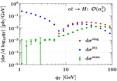
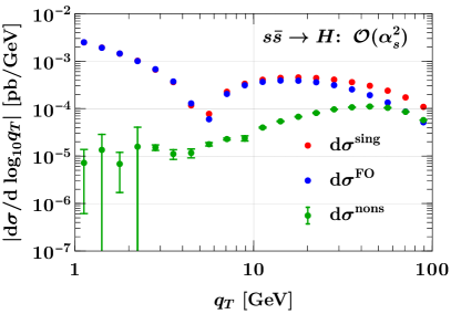
Figure -1185: Singular (solid red), full (dashed blue), and nonsingular (dotted green) contributions for $c\bar{c}\to H$ (left) and $s\bar{s}\to H$ (right) at fixed $\mathcal{O}(\alpha_{s})$ (top) and $\mathcal{O}(\alpha_{s}^{2})$ (bottom).

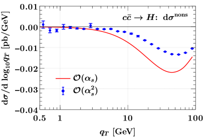
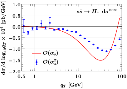
Figure -1184: Nonsingular contributions at $\mathcal{O}(\alpha_{s})$ (red) and $\mathcal{O}(\alpha_{s}^{2})$ (blue) for $c\bar{c}\to H$ (left) and $s\bar{s}\to H$ (right), corresponding respectively to the green curves and points in figure -1185.

In figures -1199 and -1198 in section 3.1, we showed the $\mathcal{O}(\alpha_{s})$ and $\mathcal{O}(\alpha_{s}^{2})$ nonsingular corrections for $b\bar{b}\to H$. For completeness, here we provide the analogous plots for $c\bar{c}\to H$ and $s\bar{s}\to H$ on a logarithmic scale in figure -1185 and on a linear scale in figure -1184. In both cases we observe the expected power suppression of the nonsingular similar to $b\bar{b}\to H$, which provides an important validation of our implementation of the LO₁ and NLO₁ fixed-order results.

Appendix C Impact of factorization scale and PDF choices

In the context of $b\bar{b}\to H$, fixed-order predictions often use a low factorization scale $\mu_{F}=m_{H}/2$ or even $\mu_{F}=m_{H}/4$. For completeness, we therefore also give results for $b\bar{b}\to H$ at these lower values for the central factorization scale. We implement this by taking $w_{F}=-1$ or $w_{F}=-2$ as central choice in eq. (2.4). Figure -1183 shows the convergence of the resummed contribution to the $q_{T}$ spectrum at NLL (yellow), NNLL (green), N³LL (blue), and N³LL^′ (red) for $\mu_{F}=m_{H}/2$ (left) and $\mu_{F}=m_{H}/4$ (right). While the convergence pattern of subsequent orders is acceptable in all cases, both the corrections and perturbative uncertainties are somewhat larger for $\mu_{F}=m_{H}/2$ than for $\mu_{F}=m_{H}$, and substantially larger for $\mu_{F}=m_{H}/4$. In our context these lower choices are therefore clearly less preferable.

In figure -1182, we assess the impact of changing the PDF set from MSHT20nnlo to MSHT20an3lo. The left panel shows the $q_{T}$ spectrum at different resummation orders for the MSHT20an3lo PDF set. As expected, the perturbative convergence is equally good as for our default choice in figure -1190. The right panel shows the highest order (N³LL^′+N³LO) for both PDF sets normalized to our default MSHT20nnlo set. Although the difference for the $b$-quark PDF between the two sets is quite significant, this is not reflected in our final results for the $q_{T}$ spectrum. The largest difference appears below $q_{T}\lesssim 20\,\mathrm{GeV}$, where the MSHT20an3lo PDF leads to a 5-10% increase in the spectrum.

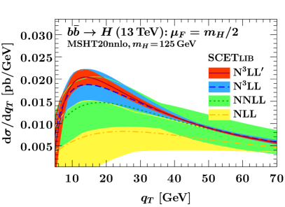
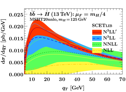
Figure -1183: The purely resummed result for $b\bar{b}\to H$ at different orders for different values of $\mu_{F}$.

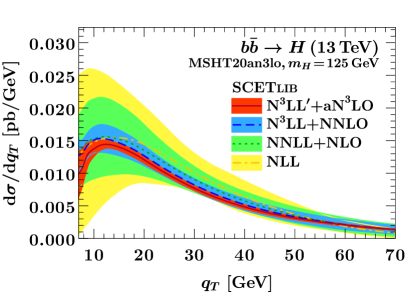
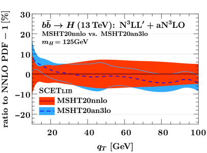
Figure -1182: Comparison of the MSHT20nnlo and the MSHT20an3lo PDF sets for $b\bar{b}\to H$.

References

- [1] ATLAS collaboration, Observation of a new particle in the search for the Standard Model Higgs boson with the ATLAS detector at the LHC, Phys. Lett. B 716 (2012) 1 [1207.7214].
- [2] CMS collaboration, Observation of a New Boson at a Mass of 125 GeV with the CMS Experiment at the LHC, Phys. Lett. B 716 (2012) 30 [1207.7235].
- [3] ATLAS collaboration, Observation of decays and production with the ATLAS detector, Phys. Lett. B 786 (2018) 59 [1808.08238].
- [4] ATLAS collaboration, Observation of Higgs boson production in association with a top quark pair at the LHC with the ATLAS detector, Phys. Lett. B 784 (2018) 173 [1806.00425].
- [5] CMS collaboration, Observation of H production, Phys. Rev. Lett. 120 (2018) 231801 [1804.02610].
- [6] ATLAS collaboration, A detailed map of Higgs boson interactions by the ATLAS experiment ten years after the discovery, Nature 607 (2022) 52 [2207.00092].
- [7] ATLAS collaboration, Combined measurements of Higgs boson production and decay using up to fb-1 of proton-proton collision data at TeV collected with the ATLAS experiment, .
- [8] CMS collaboration, Observation of Higgs boson decay to bottom quarks, Phys. Rev. Lett. 121 (2018) 121801 [1808.08242].
- [9] ATLAS collaboration, Search for the Decay of the Higgs Boson to Charm Quarks with the ATLAS Experiment, Phys. Rev. Lett. 120 (2018) 211802 [1802.04329].
- [10] D. Dicus, T. Stelzer, Z. Sullivan and S. Willenbrock, Higgs boson production in association with bottom quarks at next-to-leading order, Phys. Rev. D 59 (1999) 094016 [hep-ph/9811492].
- [11] C. Balazs, H.-J. He and C. P. Yuan, QCD corrections to scalar production via heavy quark fusion at hadron colliders, Phys. Rev. D 60 (1999) 114001 [hep-ph/9812263].
- [12] R. V. Harlander and W. B. Kilgore, Higgs boson production in bottom quark fusion at next-to-next-to leading order, Phys. Rev. D 68 (2003) 013001 [hep-ph/0304035].
- [13] S. Dittmaier, M. Krämer and M. Spira, Higgs radiation off bottom quarks at the Tevatron and the CERN LHC, Phys. Rev. D 70 (2004) 074010 [hep-ph/0309204].
- [14] S. Dawson, C. B. Jackson, L. Reina and D. Wackeroth, Exclusive Higgs boson production with bottom quarks at hadron colliders, Phys. Rev. D 69 (2004) 074027 [hep-ph/0311067].
- [15] A. Belyaev, P. M. Nadolsky and C. P. Yuan, Transverse momentum resummation for Higgs boson produced via b anti-b fusion at hadron colliders, JHEP 04 (2006) 004 [hep-ph/0509100].
- [16] R. V. Harlander, K. J. Ozeren and M. Wiesemann, Higgs plus jet production in bottom quark annihilation at next-to-leading order, Phys. Lett. B 693 (2010) 269 [1007.5411].
- [17] R. Harlander and M. Wiesemann, Jet-veto in bottom-quark induced Higgs production at next-to-next-to-leading order, JHEP 04 (2012) 066 [1111.2182].
- [18] S. Bühler, F. Herzog, A. Lazopoulos and R. Müller, The fully differential hadronic production of a Higgs boson via bottom quark fusion at NNLO, JHEP 07 (2012) 115 [1204.4415].
- [19] R. V. Harlander, S. Liebler and H. Mantler, SusHi: A program for the calculation of Higgs production in gluon fusion and bottom-quark annihilation in the Standard Model and the MSSM, Comput. Phys. Commun. 184 (2013) 1605 [1212.3249].
- [20] R. V. Harlander, A. Tripathi and M. Wiesemann, Higgs production in bottom quark annihilation: Transverse momentum distribution at NNLONNLL, Phys. Rev. D 90 (2014) 015017 [1403.7196].
- [21] M. Wiesemann, R. Frederix, S. Frixione, V. Hirschi, F. Maltoni and P. Torrielli, Higgs production in association with bottom quarks, JHEP 02 (2015) 132 [1409.5301].
- [22] M. Bonvini, A. S. Papanastasiou and F. J. Tackmann, Resummation and matching of b-quark mass effects in production, JHEP 11 (2015) 196 [1508.03288].
- [23] M. Bonvini, A. S. Papanastasiou and F. J. Tackmann, Matched predictions for the cross section at the 13 TeV LHC, JHEP 10 (2016) 053 [1605.01733].
- [24] S. Forte, D. Napoletano and M. Ubiali, Higgs production in bottom-quark fusion in a matched scheme, Phys. Lett. B 751 (2015) 331 [1508.01529].
- [25] S. Forte, D. Napoletano and M. Ubiali, Higgs production in bottom-quark fusion: matching beyond leading order, Phys. Lett. B 763 (2016) 190 [1607.00389].
- [26] R. V. Harlander, Higgs production in heavy quark annihilation through next-to-next-to-leading order QCD, Eur. Phys. J. C 76 (2016) 252 [1512.04901].
- [27] M. Lim, F. Maltoni, G. Ridolfi and M. Ubiali, Anatomy of double heavy-quark initiated processes, JHEP 09 (2016) 132 [1605.09411].
- [28] G. Das, Higgs rapidity in bottom annihilation at NNLL and beyond, 2306.04561.
- [29] T. Gehrmann and D. Kara, The form factor to three loops in QCD, JHEP 09 (2014) 174 [1407.8114].
- [30] A. Chakraborty, T. Huber, R. N. Lee, A. von Manteuffel, R. M. Schabinger, A. V. Smirnov et al., Hbb vertex at four loops and hard matching coefficients in SCET for various currents, Phys. Rev. D 106 (2022) 074009 [2204.02422].
- [31] C. Duhr, F. Dulat and B. Mistlberger, Higgs Boson Production in Bottom-Quark Fusion to Third Order in the Strong Coupling, Phys. Rev. Lett. 125 (2020) 051804 [1904.09990].
- [32] C. Duhr, F. Dulat, V. Hirschi and B. Mistlberger, Higgs production in bottom quark fusion: matching the 4- and 5-flavour schemes to third order in the strong coupling, JHEP 08 (2020) 017 [2004.04752].
- [33] R. Mondini and C. Williams, Bottom-induced contributions to Higgs plus jet at next-to-next-to-leading order, JHEP 05 (2021) 045 [2102.05487].
- [34] D. Pagani, H.-S. Shao and M. Zaro, RIP : how other Higgs production modes conspire to kill a rare signal at the LHC, JHEP 11 (2020) 036 [2005.10277].
- [35] M. A. Ebert, S. Liebler, I. Moult, I. W. Stewart, F. J. Tackmann, K. Tackmann et al., Exploiting jet binning to identify the initial state of high-mass resonances, Phys. Rev. D 94 (2016) 051901 [1605.06114].
- [36] F. Bishara, U. Haisch, P. F. Monni and E. Re, Constraining Light-Quark Yukawa Couplings from Higgs Distributions, Phys. Rev. Lett. 118 (2017) 121801 [1606.09253].
- [37] Y. Soreq, H. X. Zhu and J. Zupan, Light quark Yukawa couplings from Higgs kinematics, JHEP 12 (2016) 045 [1606.09621].
- [38] ATLAS collaboration, Measurement of the total and differential Higgs boson production cross-sections at = 13 TeV with the ATLAS detector by combining the and decay channels, JHEP 05 (2023) 028 [2207.08615].
- [39] CMS collaboration, Measurements of inclusive and differential cross sections for the Higgs boson production and decay to four-leptons in proton-proton collisions at = 13 TeV, 2305.07532.
- [40] G. Billis, B. Dehnadi, M. A. Ebert, J. K. L. Michel and F. J. Tackmann, Higgs Spectrum and Total Cross Section with Fiducial Cuts at Third Resummed and Fixed Order in QCD, Phys. Rev. Lett. 127 (2021) 072001 [2102.08039].
- [41] S. Camarda, L. Cieri and G. Ferrera, Drell–Yan lepton-pair production: qT resummation at N3LL accuracy and fiducial cross sections at N3LO, Phys. Rev. D 104 (2021) L111503 [2103.04974].
- [42] E. Re, L. Rottoli and P. Torrielli, Fiducial Higgs and Drell-Yan distributions at N3LL′+NNLO with RadISH, 2104.07509.
- [43] W.-L. Ju and M. Schönherr, The qT and spectra in W and Z production at the LHC at N3LL’+N2LO, JHEP 10 (2021) 088 [2106.11260].
- [44] T. Neumann and J. Campbell, Fiducial Drell-Yan production at the LHC improved by transverse-momentum resummation at N4LLp+N3LO, Phys. Rev. D 107 (2023) L011506 [2207.07056].
- [45] G. Billis, M. A. Ebert, J. K. L. Michel and F. J. Tackmann, Drell-Yan Spectrum and Its Uncertainty at NLL′ and Approximate NLL, DESY-23-081, MIT-CTP 5572 (2023) , in preparation.
- [46] C. W. Bauer, S. Fleming, D. Pirjol and I. W. Stewart, An Effective field theory for collinear and soft gluons: Heavy to light decays, Phys. Rev. D 63 (2001) 114020 [hep-ph/0011336].
- [47] C. W. Bauer and I. W. Stewart, Invariant operators in collinear effective theory, Phys. Lett. B 516 (2001) 134 [hep-ph/0107001].
- [48] C. W. Bauer, D. Pirjol and I. W. Stewart, Soft collinear factorization in effective field theory, Phys. Rev. D 65 (2002) 054022 [hep-ph/0109045].
- [49] C. W. Bauer, S. Fleming, D. Pirjol, I. Z. Rothstein and I. W. Stewart, Hard scattering factorization from effective field theory, Phys. Rev. D 66 (2002) 014017 [hep-ph/0202088].
- [50] M. Beneke, A. P. Chapovsky, M. Diehl and T. Feldmann, Soft collinear effective theory and heavy to light currents beyond leading power, Nucl. Phys. B 643 (2002) 431 [hep-ph/0206152].
- [51] P. Pietrulewicz, D. Samitz, A. Spiering and F. J. Tackmann, Factorization and Resummation for Massive Quark Effects in Exclusive Drell-Yan, JHEP 08 (2017) 114 [1703.09702].
- [52] B. Dehnadi, I. Novikov and F. J. Tackmann, The photon energy spectrum in at N3LL′, 2211.07663.
- [53] J. C. Collins and D. E. Soper, Back-To-Back Jets in QCD, Nucl. Phys. B 193 (1981) 381.
- [54] J. C. Collins and D. E. Soper, Back-To-Back Jets: Fourier Transform from B to K-Transverse, Nucl. Phys. B 197 (1982) 446.
- [55] J. C. Collins, D. E. Soper and G. F. Sterman, Transverse Momentum Distribution in Drell-Yan Pair and W and Z Boson Production, Nucl. Phys. B 250 (1985) 199.
- [56] S. Catani, D. de Florian and M. Grazzini, Universality of nonleading logarithmic contributions in transverse momentum distributions, Nucl. Phys. B 596 (2001) 299 [hep-ph/0008184].
- [57] D. de Florian and M. Grazzini, The Structure of large logarithmic corrections at small transverse momentum in hadronic collisions, Nucl. Phys. B 616 (2001) 247 [hep-ph/0108273].
- [58] J. Collins, Foundations of perturbative QCD, vol. 32. Cambridge University Press, 11, 2013.
- [59] T. Becher and M. Neubert, Drell-Yan Production at Small , Transverse Parton Distributions and the Collinear Anomaly, Eur. Phys. J. C 71 (2011) 1665 [1007.4005].
- [60] M. G. Echevarria, A. Idilbi and I. Scimemi, Factorization Theorem For Drell-Yan At Low And Transverse Momentum Distributions On-The-Light-Cone, JHEP 07 (2012) 002 [1111.4996].
- [61] J.-Y. Chiu, A. Jain, D. Neill and I. Z. Rothstein, A Formalism for the Systematic Treatment of Rapidity Logarithms in Quantum Field Theory, JHEP 05 (2012) 084 [1202.0814].
- [62] Y. Li, D. Neill and H. X. Zhu, An exponential regulator for rapidity divergences, Nucl. Phys. B 960 (2020) 115193 [1604.00392].
- [63] M. A. Ebert and F. J. Tackmann, Resummation of Transverse Momentum Distributions in Distribution Space, JHEP 02 (2017) 110 [1611.08610].
- [64] M. A. Ebert, J. K. L. Michel, I. W. Stewart and F. J. Tackmann, Drell-Yan resummation of fiducial power corrections at N3LL, JHEP 04 (2021) 102 [2006.11382].
- [65] M. A. Ebert, J. K. L. Michel and F. J. Tackmann, Resummation Improved Rapidity Spectrum for Gluon Fusion Higgs Production, JHEP 05 (2017) 088 [1702.00794].
- [66] T. Lübbert, J. Oredsson and M. Stahlhofen, Rapidity renormalized TMD soft and beam functions at two loops, JHEP 03 (2016) 168 [1602.01829].
- [67] Y. Li and H. X. Zhu, Bootstrapping Rapidity Anomalous Dimensions for Transverse-Momentum Resummation, Phys. Rev. Lett. 118 (2017) 022004 [1604.01404].
- [68] G. Billis, M. A. Ebert, J. K. L. Michel and F. J. Tackmann, A toolbox for and 0-jettiness subtractions at , Eur. Phys. J. Plus 136 (2021) 214 [1909.00811].
- [69] M.-x. Luo, T.-Z. Yang, H. X. Zhu and Y. J. Zhu, Quark Transverse Parton Distribution at the Next-to-Next-to-Next-to-Leading Order, Phys. Rev. Lett. 124 (2020) 092001 [1912.05778].
- [70] M. A. Ebert, B. Mistlberger and G. Vita, Transverse momentum dependent PDFs at N3LO, JHEP 09 (2020) 146 [2006.05329].
- [71] S. Moch, J. A. M. Vermaseren and A. Vogt, The Quark form-factor at higher orders, JHEP 08 (2005) 049 [hep-ph/0507039].
- [72] I. W. Stewart, F. J. Tackmann and W. J. Waalewijn, The Quark Beam Function at NNLL, JHEP 09 (2010) 005 [1002.2213].
- [73] R. Brüser, Z. L. Liu and M. Stahlhofen, Three-Loop Quark Jet Function, Phys. Rev. Lett. 121 (2018) 072003 [1804.09722].
- [74] A. A. Vladimirov, Correspondence between Soft and Rapidity Anomalous Dimensions, Phys. Rev. Lett. 118 (2017) 062001 [1610.05791].
- [75] G. P. Korchemsky and A. V. Radyushkin, Renormalization of the Wilson Loops Beyond the Leading Order, Nucl. Phys. B283 (1987) 342.
- [76] S. Moch, J. A. M. Vermaseren and A. Vogt, The Three loop splitting functions in QCD: The Nonsinglet case, Nucl. Phys. B688 (2004) 101 [hep-ph/0403192].
- [77] R. Brüser, A. Grozin, J. M. Henn and M. Stahlhofen, Matter dependence of the four-loop QCD cusp anomalous dimension: from small angles to all angles, JHEP 05 (2019) 186 [1902.05076].
- [78] J. M. Henn, G. P. Korchemsky and B. Mistlberger, The full four-loop cusp anomalous dimension in super Yang-Mills and QCD, JHEP 04 (2020) 018 [1911.10174].
- [79] A. von Manteuffel, E. Panzer and R. M. Schabinger, Analytic four-loop anomalous dimensions in massless QCD from form factors, Phys. Rev. Lett. 124 (2020) 162001 [2002.04617].
- [80] O. V. Tarasov, A. A. Vladimirov and A. Yu. Zharkov, The Gell-Mann-Low Function of QCD in the Three Loop Approximation, Phys. Lett. 93B (1980) 429.
- [81] S. A. Larin and J. A. M. Vermaseren, The Three loop QCD Beta function and anomalous dimensions, Phys. Lett. B303 (1993) 334 [hep-ph/9302208].
- [82] T. van Ritbergen, J. A. M. Vermaseren and S. A. Larin, The Four loop beta function in quantum chromodynamics, Phys. Lett. B400 (1997) 379 [hep-ph/9701390].
- [83] M. Czakon, The Four-loop QCD beta-function and anomalous dimensions, Nucl. Phys. B710 (2005) 485 [hep-ph/0411261].
- [84] G. Lustermans, J. K. L. Michel, F. J. Tackmann and W. J. Waalewijn, Joint two-dimensional resummation in and -jettiness at NNLL, JHEP 03 (2019) 124 [1901.03331].
- [85] Z. Ligeti, I. W. Stewart and F. J. Tackmann, Treating the b quark distribution function with reliable uncertainties, Phys. Rev. D 78 (2008) 114014 [0807.1926].
- [86] R. Abbate, M. Fickinger, A. H. Hoang, V. Mateu and I. W. Stewart, Thrust at with Power Corrections and a Precision Global Fit for , Phys. Rev. D 83 (2011) 074021 [1006.3080].
- [87] I. W. Stewart, F. J. Tackmann, J. R. Walsh and S. Zuberi, Jet resummation in Higgs production at , Phys. Rev. D 89 (2014) 054001 [1307.1808].
- [88] M. A. Ebert, J. K. L. Michel, F. J. Tackmann et al., SCETlib: A C++ Package for Numerical Calculations in QCD and Soft-Collinear Effective Theory, DESY-17-099 (2018) .
- [89] S. Alioli, C. W. Bauer, C. Berggren, F. J. Tackmann and J. R. Walsh, Drell-Yan production at NNLL’+NNLO matched to parton showers, Phys. Rev. D 92 (2015) 094020 [1508.01475].
- [90] S. Alioli, G. Billis, A. Broggio, A. Gavardi, S. Kallweit, M. A. Lim et al., Refining the GENEVA method for Higgs boson production via gluon fusion, JHEP 05 (2023) 128 [2301.11875].
- [91] S. Frixione, Z. Kunszt and A. Signer, Three jet cross-sections to next-to-leading order, Nucl. Phys. B 467 (1996) 399 [hep-ph/9512328].
- [92] V. Del Duca, C. Duhr, G. Somogyi, F. Tramontano and Z. Trócsányi, Higgs boson decay into b-quarks at NNLO accuracy, JHEP 04 (2015) 036 [1501.07226].
- [93] S. Alioli, A. Broggio, A. Gavardi, S. Kallweit, M. A. Lim, R. Nagar et al., Resummed predictions for hadronic Higgs boson decays, JHEP 04 (2021) 254 [2009.13533].
- [94] OpenLoops 2 collaboration, F. Buccioni, J.-N. Lang, J. M. Lindert, P. Maierhöfer, S. Pozzorini, H. Zhang et al., OpenLoops 2, Eur. Phys. J. C 79 (2019) 866 [1907.13071].
- [95] J. Gaunt, M. Stahlhofen, F. J. Tackmann and J. R. Walsh, N-jettiness Subtractions for NNLO QCD Calculations, JHEP 09 (2015) 058 [1505.04794].
- [96] R. Boughezal, C. Focke, X. Liu and F. Petriello, -boson production in association with a jet at next-to-next-to-leading order in perturbative QCD, Phys. Rev. Lett. 115 (2015) 062002 [1504.02131].
- [97] M. A. Ebert, I. Moult, I. W. Stewart, F. J. Tackmann, G. Vita and H. X. Zhu, Subleading power rapidity divergences and power corrections for qT, JHEP 04 (2019) 123 [1812.08189].
- [98] S. Bailey, T. Cridge, L. A. Harland-Lang, A. D. Martin and R. S. Thorne, Parton distributions from LHC, HERA, Tevatron and fixed target data: MSHT20 PDFs, Eur. Phys. J. C 81 (2021) 341 [2012.04684].
- [99] J. McGowan, T. Cridge, L. A. Harland-Lang and R. S. Thorne, Approximate N3LO parton distribution functions with theoretical uncertainties: MSHT20aN3LO PDFs, Eur. Phys. J. C 83 (2023) 185 [2207.04739].
- [100] Particle Data Group collaboration, R. L. Workman and Others, Review of Particle Physics, PTEP 2022 (2022) 083C01.
- [101] M. A. Ebert and F. J. Tackmann, Impact of isolation and fiducial cuts on qT and N-jettiness subtractions, JHEP 03 (2020) 158 [1911.08486].