Neural Networks can detect
model-free static arbitrage strategies

Abstract.

In this paper we demonstrate both theoretically as well as numerically that neural networks can detect model-free static arbitrage opportunities whenever the market admits some. Due to the use of neural networks, our method can be applied to financial markets with a high number of traded securities and ensures almost immediate execution of the corresponding trading strategies. To demonstrate its tractability, effectiveness, and robustness we provide examples using real financial data. From a technical point of view, we prove that a single neural network can approximately solve a class of convex semi-infinite programs, which is the key result in order to derive our theoretical results that neural networks can detect model-free static arbitrage strategies whenever the financial market admits such opportunities.

Keywords: Static Arbitrage, Model-Free Finance, Deep Learning, Convex Optimization

¹NTU Singapore, Division of Mathematical Sciences,
21 Nanyang Link, Singapore 637371.
²National University of Singapore, Department of Mathematics,
21 Lower Kent Ridge Road, 119077.

1. Introduction

Detecting arbitrage opportunities in financial markets and efficiently implementing them numerically is an intricate and demanding task, both in theory and practice. In recent academic papers, researchers have extensively tackled this problem for various types of assets, highlighting its significance and complexity.

The authors from cui2020detecting and cui2020arbitrage focus their studies on the foreign exchange market, establish conditions that eliminate triangular opportunities and propose computational approaches to detect arbitrage opportunities.

soon2011currency propose a binary integer programming model for the detection of arbitrage in currency exchange markets, while papapantoleon2021detection focus on arbitrage in multi-asset markets under the assumptions that the risk-neutral marginal distributions are known. Also assuming knowledge of risk-neutral marginals in multi-asset markets, tavin2015detection provides a copula-based approach to characterize the absence of arbitrage. cohen2020detecting study arbitrage opportunities in markets where vanilla options are traded and propose an efficient procedure to change the option prices minimally (w.r.t. the $\l^{1}$ distance) such that the market becomes arbitrage-free. neufeld2022model develop cutting-plane based algorithms to calculate model free upper and lower price bounds whose sub-optimality can be chosen to be arbitrarily small, and use them to detect model-free arbitrage strategies. Furthermore, by observing call option prices biagini2022detecting train neural networks to detect financial asset bubbles.

In this paper we study the detection of model-free static arbitrage in potentially high-dimensional financial markets, i.e., in markets where a large number of securities are traded. A trading strategy is called static if the strategy consists of buying or selling financial derivatives as well as the corresponding underlying securities in the market only at initial time (with corresponding bid and ask prices) and then holding the positions till maturity without any readjustment. Therefore, one says that a market admits static arbitrage if there exists a static trading strategy which provides a guaranteed risk-free profit at maturity. We aim to detect static arbitrage opportunities in a model-free way, i.e. purely based on observable market data without imposing any (probabilistic) model assumptions on the underlying financial market. We also refer to acciaio2016model; Burzoni; burzoni2019pointwise; burzoni2021viability; cheridito2017duality; davis2014arbitrage; fahim2016model; hobson2005static; hobson2005static2; neufeld2022deep; riedel2015financial; wang2021necessary for more details on model-free arbitrage and its characterization.

The goal of this paper is to demonstrate both theoretically as well as numerically using real-market data that neural networks can detect model-free static arbitrage whenever the market admits some. The motivation of using neural networks is their known ability to efficiently deal with high-dimensional problems in various fields. There are several algorithms that can detect (static) arbitrage strategies in a financial market under fixed market conditions, for example in a market with fixed options with corresponding strikes as well as fixed corresponding bid and ask prices. However directly applying these algorithms in real financial market scenarios to exploit arbitrage is challenging due to well-known issue that market conditions changes extremely fast and high-frequency trading often cause these opportunities to vanish rapidly. This associated risk is commonly known as execution risk, as discussed, e.g., in kozhan2012execution. The speed of investment execution therefore becomes crucial in capitalizing on arbitrage opportunities.

By training neural networks according to our algorithm purely based on observed market data, we obtain detectors that allow, given any market conditions, to detect not only the existence of static arbitrage but also to determine a proper applicable arbitrage strategy. Our algorithm therefore provides to financial agents an instruction how to trade and to exploit the arbitrage strategy while the opportunity persists. In contrast to other numerical methods which need to be executed entirely each time the market is scanned for arbitrage or the market conditions are changing, our proposed method only needs one neural network to be trained offline. After training, the neural network is then able to detect arbitrage and can be executed extremely fast, allowing to invest in the resultant strategies in every new market situation that one faces. We refer to Section 3 for detailed description of our algorithm as well as our numerical results evaluated on real market data.

We justify the use of neural networks by proving that neural networks can detect model-free static arbitrage strategies whenever the market admits some. We refer to Theorem 2.5 and Theorem 2.6 for our main theoretical results regarding arbitrage detection. The main idea is to relate arbitrage with the superhedging of the zero-payoff function. We prove in Proposition 2.7 that there exists a single neural network that provides a corresponding $\varepsilon$-optimal superhedging strategy for any given market conditions. In fact, we show for a certain class of convex semi-infinite programs (CSIP), which includes the superhedging problem of the zero-payoff function as special case, that a single neural network can provide for each of the (CSIP) within this class a corresponding feasible and $\varepsilon$-optimal solution, see Theorem 4.5.

The remainder of this paper is as follows. In Section 2, we introduce the setting of the financial market as well as the corresponding (static) trading strategies, and provide our main theoretical results ensuring that model-free static arbitrage can be detected by neural networks if existent. Section 3 focuses on the presentation and numerical implementation of our neural networks based algorithm to detect static arbitrage, featuring experiments conducted on real financial data to showcase the feasibility and robustness of our method. In Section 4, we introduce a class of convex semi-infinite programs and provide our main technical result that a single neural network can approximately solve this class of (CSIPs). Finally, all proofs are presented in Section 5.

2. Detection of static Arbitrage Strategies

In this section, we study a financial market in which a financial agent can trade statically in various types of options and which may admit the opportunity of static arbitrage profits. In such a setting, the natural difficulty for a trader is first to decide whether such arbitrage exists and second to identify potential strategies that exploit arbitrage profits. Our goal is to show that for each financial market in which an agent can trade statically in options, the corresponding market admits static arbitrage if and only if there exists a neural network that detects the existence of model-free static arbitrage by outputting a corresponding arbitrage strategy.

2.1. Setting

In this paper, we consider a market in which a financial agent can trade statically in options. To introduce the market under consideration, let $S=(S_{1},\dots,S_{d})$ denote the underlying $d\in\mathbb{N}$ stocks at some future time $t=1$. We only consider values $S\in\mathcal{S}\subseteq[0,\infty)^{d}$ for some predefined set $\mathcal{S}$, which can be interpreted as prediction set where the financial agent may allow to exclude values which she considers to be impossible to model future stock prices $S=(S_{1},\dots,S_{d})$ at time $1$.

Let $N_{\Psi}\in\mathbb{N}$ denote the number of different types of traded options $\Psi_{i}:\mathcal{S}\times[0,\overline{K}]\rightarrow[0,\infty)$, $i=1,\dots,N_{\Psi}$, written on $S$. For each option type $i\in\{1,\dots,N_{\Psi}\}$ let $n_{i}\in\mathbb{N}$ denote the corresponding amount of different strikes under consideration $(K_{i,j})_{j=1,\dots,n_{i}}\subseteq[0,\overline{K}]$, where the strikes are contained in $[0,\overline{K}]$ for some $\overline{K}<\infty$, and denote by $N:=\sum_{i=1}^{N_{\Psi}}n_{i}$ the total number of traded options. Moreover, we denote by $\pi=(\pi_{i,j})_{i=1,\dots,N_{\Psi},\atop j=1,\dots,n_{i}}=(\pi_{i,j}^{+},\pi_{i,j}^{-})_{i=1,\dots,N_{\Psi},\atop j=1,\dots,n_{i}}\in[0,\overline{\pi}]^{2N}$ the bid and ask prices of the traded options respectively, where we assume that all the bid and ask prices are bounded by some $\overline{\pi}>0$.

The financial agent then can trade in the market by buying and selling the options described above. More precisely, we first fix the minimal initial cash position of a trading strategy to be given by $\underline{a}\in\mathbb{R}$, and we assume that the maximal amount of shares of options one can buy or sell is capped by some constant $0<\overline{H}<\infty$. This allows to consider the payoff of a static trading strategy by the function

(2.1) $$\mathcal{I}_{S}:[0,\overline{K}]^{N}\times[\underline{a},\infty)\times[0,\overline{H}]^{2N} \rightarrow\mathbb{R}$$

$$(K,a,h) \mapsto a+\sum_{i=1}^{N_{\Psi}}\sum_{j=1}^{n_{i}}\left(h_{i,j}^{+}-h_{i,j}^{-}\right)\cdot\Psi_{i}(S,K_{i,j}),$$

where we use the notation $h=\left(h_{i,j}^{+},h_{i,j}^{-}\right)_{i=1,\dots,N_{\Psi},\atop j=1,\dots,n_{i}}\in[0,\overline{H}]^{2N}$ to denote long and short positions in the traded options, respectively, as well as $K=(K_{i,j})_{i=1,\dots,N_{\Psi},\atop j=1,\dots,n_{i}}$ to denote all strikes. The corresponding pricing functional is then defined by

(2.2) $$f:[0,\overline{\pi}]^{2N}\times[\underline{a},\infty)\times[0,\overline{H}]^{2N} \rightarrow\mathbb{R}$$

$$\left(\pi,a,h\right) \mapsto a+\sum_{i=1}^{N_{\Psi}}\sum_{j=1}^{n_{i}}\left(h_{i,j}^{+}\pi_{i,j}^{+}-h_{i,j}^{-}\pi_{i,j}^{-}\right)$$

determining the price of a corresponding trading strategy with respect to the corresponding bid and ask prices of the options.

Moreover, we define the set-valued map which maps a set of strikes $K=(K_{i,j})_{i=1,\dots,N_{\Psi},\atop j=1,\dots,n_{i}}$ to the corresponding strategies leading to a greater payoff than $0$ for each possible value $S\in\mathcal{S}$ by

(2.3) $$\Gamma:[0,\overline{K}]^{N}\ni K\twoheadrightarrow\Gamma(K):=\left\{(a,h)\in[\underline{a},\infty)\times[0,\overline{H}]^{2N}\leavevmode\nobreak\ \middle|\leavevmode\nobreak\ \mathcal{I}_{S}(K,a,h)\geq 0\text{ for all }S\in\mathcal{S}\right\}.$$

Then, the minimal price of a trading strategy that leads to a greater price than $0$ for each possible value $S\in\mathcal{S}$, in dependence of strikes $K=(K_{i,j})_{i=1,\dots,N_{\Psi},\atop j=1,\dots,n_{i}}$ and option prices $\pi=(\pi_{i,j}^{+},\pi_{i,j}^{-})_{i=1,\dots,N_{\Psi},\atop j=1,\dots,n_{i}}$, is given by

(2.4) $$V:[0,\overline{K}]^{N}\times[0,\overline{\pi}]^{2N} \rightarrow\mathbb{R}$$

$$(K,\pi) \mapsto\inf_{(a,h)\in\Gamma(K)}f(\pi,a,h).$$

In this paper, we consider the following type of model-free static arbitrage. We refer to burzoni2019pointwise for several notions of model-free arbitrage.

Definition 2.1 (Model-free static arbitrage).

Let $(K,\pi)\in[0,\overline{K}]^{N}\times[0,\overline{\pi}]^{2N}$. Then, we call a static trading strategy $(a,h)\in[\underline{a},\infty)\times[0,\overline{H}]^{2N}$ a model-free static arbitrage strategy if the following two conditions hold.

• $(a,h)\in\Gamma(K)$,

• $f(\pi,a,h)<0$.

Moreover, for any $\varepsilon>0$ we call a model-free static arbitrage strategy to be of magnitude $\varepsilon$ if $f(\pi,a,h)\leq-\varepsilon$.

This means according to Definition 2.1 that the market with parameters $(K,\pi)\in[0,\overline{K}]^{N}\times[0,\overline{\pi}]^{2N}$ admits no model-free static arbitrage strategy if and only if $V(K,\pi)\geq 0$.

Neural Networks

By neural networks with input dimension $d_{\operatorname{in}}\in\mathbb{N}$, output dimension $d_{\operatorname{out}}\in\mathbb{N}$, and number of layers $l\in\mathbb{N}$ we refer to functions of the form

(2.5) $$\mathbb{R}^{d_{\operatorname{in}}} \rightarrow\mathbb{R}^{d_{\operatorname{out}}}$$

$${x} \mapsto{A_{l}}\circ{\varphi}_{l}\circ{A_{l-1}}\circ\cdots\circ{\varphi}_{1}\circ{A_{0}}({x}),$$

where $({A_{i}})_{i=0,\dots,l}$ are affine functions of the form

(2.6) $${A_{0}}:\mathbb{R}^{d_{{\operatorname{in}}}}\rightarrow\mathbb{R}^{h_{1}},\qquad{A_{i}}:\mathbb{R}^{h_{i}}\rightarrow\mathbb{R}^{h_{i+1}}\text{ for }i=1,\dots,l-1,\text{(if }l>1),\text{ and}\qquad{A_{l}}:\mathbb{R}^{h_{l}}\rightarrow\mathbb{R}^{d_{\operatorname{out}}},$$

and where the function $\varphi_{i}$ is applied componentwise, i.e., for $i=1,\dots,l$ we have ${\varphi}_{i}(x_{1},\dots,x_{h_{i}})=\left(\varphi(x_{1}),\dots,\varphi(x_{h_{i}})\right)$. The function $\varphi:\mathbb{R}\rightarrow\mathbb{R}$ is called activation function and assumed to be continuous and non-polynomial. We say a neural network is deep if $l\geq 2$. Here ${h}=(h_{1},\dots,h_{l})\in\mathbb{N}^{l}$ denotes the dimensions (the number of neurons) of the hidden layers, also called hidden dimension.

Then, we denote by $\mathfrak{N}_{d_{\operatorname{in}},{d_{\operatorname{out}}}}^{l,{h}}$ the set of all neural networks with input dimension ${d_{\operatorname{in}}}$, output dimension ${d_{\operatorname{out}}}$, $l$ hidden layers, and hidden dimension ${h}$, whereas the set of all neural networks from $\mathbb{R}^{d_{\operatorname{in}}}$ to $\mathbb{R}^{d_{\operatorname{out}}}$ (i.e. without specifying the number of hidden layers and hidden dimension) is denoted by

$$\mathfrak{N}_{d_{\operatorname{in}},{d_{\operatorname{out}}}}:=\bigcup_{l\in\mathbb{N}}\bigcup_{{h}\in\mathbb{N}^{l}}\mathfrak{N}_{d_{\operatorname{in}},{d_{\operatorname{out}}}}^{l,{h}}.$$

It is well-known that the set of neural networks possess the so-called universal approximation property, see, e.g., pinkus1999approximation.

Proposition 2.2 (Universal approximation theorem).

For any compact set $\mathbb{K}\subset\mathbb{R}^{d_{\operatorname{in}}}$ the set $\mathfrak{N}_{d_{\operatorname{in}},{d_{\operatorname{out}}}}|_{\mathbb{K}}$ is dense in ${C}(\mathbb{K},\mathbb{R}^{d_{\operatorname{out}}})$ with respect to the topology of uniform convergence on $C(\mathbb{K},\mathbb{R}^{d_{\operatorname{out}}})$.

2.2. Main results

To formulate our main result we first impose the following mild assumptions.

Assumption 2.3.

• There exists some $L_{\Psi}>0$ such that for all $S\in\mathcal{S}$ and for all $i=1,\dots,N_{\Psi}$ the map $[0,\overline{K}]\ni K_{i,j}\mapsto\Psi_{i}(S,K_{i,j})$ is $L_{\Psi}$-Lipschitz.

• There exists some by $C_{\Psi}>0$ such that the map $\Psi_{i}$ is bounded by $C_{\Psi}$ on $\mathcal{S}\times[0,\overline{K}]$ for all $i=1,\dots,N_{\Psi}$.

Remark 2.4.

First, note that we do not impose any topological or geometric conditions on the prediction set $\mathcal{S}\subset[0,\infty)^{d}$. However, a sufficient criterion for Assumption 2.3 (ii) to hold would be that, e.g., $\mathcal{S}\subset[0,\infty)^{d}$ is bounded and that $[0,\infty)^{d}\times[0,\overline{K}]\ni(S,K)\mapsto\Psi_{i}(S,K)$ is continuous for each $i=1,\dots,N_{\Psi}$. Moreover, note that Assumption 2.3 (i) is satisfied for example for any payoff function which is continuous and piece-wise affine (CPWA), which includes most relevant payoff functions in finance. We refer to neufeld2022model; li2023quantum for a detailed list of examples of (CPWA) payoff functions.

In our first result, we conclude that the financial market described in Section 2.1 admits model-free static arbitrage if and only if there exists a neural network that detects the existence of model-free static arbitrage by outputting a corresponding arbitrage strategy.

Theorem 2.5 (Neural networks can detect static arbitrage).

Let Assumption 2.3 hold true, and let $(K,\pi)\in[0,\overline{K}]^{N}\times[0,\overline{\pi}]^{2N}$. Then, there exists model-free static arbitrage if and only if there exists a neural network $\mathcal{N}\mathcal{N}\in\mathfrak{N}_{3N,1+2N}$ with

• $\mathcal{N}\mathcal{N}(K,\pi):=\left(\mathcal{N}\mathcal{N}_{a}(K,\pi),\mathcal{N}\mathcal{N}_{h}(K,\pi)\right)\in\Gamma(K)$,

• $f\left(\pi,\mathcal{N}\mathcal{N}_{a}(K,\pi),\mathcal{N}\mathcal{N}_{h}(K,\pi)\right)<0$.

In our second result, we show that for any given $\varepsilon>0$ and $0<\delta<\varepsilon$ there exists a single neural network such that for any given strikes $K=(K_{i,j})_{i=1,\dots,N_{\Psi},\atop j=1,\dots,n_{i}}$ and option prices $\pi=(\pi_{i,j}^{+},\pi_{i,j}^{-})_{i=1,\dots,N_{\Psi},\atop j=1,\dots,n_{i}}$ the neural network can detect model-free static arbitrage of magnitude $\delta$ if the financial market with corresponding market conditions $(K,\pi)$ admits static arbitrage of magnitude $\varepsilon$. From a practical point of view, this is crucial, since it allows the financial trader to only train one single neural network which can then, once trained, instantaneously detect corresponding static arbitrage opportunities if the current market conditions $(K,\pi)$ admit such opportunities. On the other hand, a trader applying the trained neural network to a financial market which admits no static arbitrage opportunities pays at most $\varepsilon-\delta$ for the trading strategy, i.e., if $\varepsilon\approx\delta$, the risk of paying for trading strategies which are no static arbitrage strategies can be reduced to an arbitrarily small amount.

Theorem 2.6 (A single neural network can detect static arbitrage of magnitude $\varepsilon$).

Let $\varepsilon>0$ and $0<\delta<\varepsilon$. Then, there exists a neural $\mathcal{N}\mathcal{N}\in\mathfrak{N}_{3N,1+2N}$ such that for every $(K,\pi)\in[0,\overline{K}]^{N}\times[0,\overline{\pi}]^{2N}$ the following holds.

• If the financial market with respect to $(K,\pi)$ admits model-free static arbitrage of magnitude $\varepsilon$, then the neural network outputs a trading strategy $\left(\mathcal{N}\mathcal{N}_{a}(K,\pi),\mathcal{N}\mathcal{N}_{h}(K,\pi)\right)$ which is a model-free static arbitrage of magnitude $\delta$.

• If the financial market with respect to $(K,\pi)$ admits no model-free static arbitrage, then the neural network outputs a trading strategy $\left(\mathcal{N}\mathcal{N}_{a}(K,\pi),\mathcal{N}\mathcal{N}_{h}(K,\pi)\right)\in\Gamma(K)$ which has a price of at most $\varepsilon-\delta$.

The main idea to derive Theorem 2.5 and Theorem 2.6 relies on the relation between arbitrage and supehedging of the $0$-payoff function. The following result establishes that for any prescribed $\varepsilon>0$ there exists a single neural network such that for any given strikes $K=(K_{i,j})_{i=1,\dots,N_{\Psi},\atop j=1,\dots,n_{i}}$ and option prices $\pi=(\pi_{i,j}^{+},\pi_{i,j}^{-})_{i=1,\dots,N_{\Psi},\atop j=1,\dots,n_{i}}$ defining the market, the neural network produces a static trading strategy which superhedges the $0$-payoff for all possible values $S\in\mathcal{S}$ whose price is $\varepsilon$-optimal.

Proposition 2.7 (Approximating $V$ with neural networks).

Let Assumption 2.3 hold true. Then for all $\varepsilon>0$ there exists a neural network $\mathcal{N}\mathcal{N}\in\mathfrak{N}_{3N,1+2N}$ such that

• $\mathcal{N}\mathcal{N}(K,\pi):=\left(\mathcal{N}\mathcal{N}_{a}(K,\pi),\mathcal{N}\mathcal{N}_{h}(K,\pi)\right)\in\Gamma(K)$ for all $(K,\pi)\in[0,\overline{K}]^{N}\times[0,\overline{\pi}]^{2N}$,

• $f\left(\pi,\mathcal{N}\mathcal{N}_{a}(K,\pi),\mathcal{N}\mathcal{N}_{h}(K,\pi)\right)-V(K,\pi)\leq\varepsilon$ for all $(K,\pi)\in[0,\overline{K}]^{N}\times[0,\overline{\pi}]^{2N}$.

In fact, we will use Proposition 2.7 to prove our main results Theorem 2.5 and Theorem 2.6 on detecting static arbitrage strategies. To prove Proposition 2.7, we interpret (2.4) as a class of linear semi-infinite optimization problem (LSIP), where each $(K,\pi)\in[0,\overline{K}]^{N}\times[0,\overline{\pi}]^{2N}$ determines a single (LSIP). In Section 3, we introduce a (much more) general class of convex semi-infinite optimization problem (CSIP) which covers (2.4) as special case. Then we show that a single neural network can approximately solve all (CSIP) of this class simultaneously. We refer to Theorem 4.5 for the precise statement.

The proofs of all our main results are provided in Section 5.

3. The Numerics of Static Arbitrage Detection in Financial Markets

The results from Section 2 prove, with non-constructive arguments, the existence of neural networks that can detect model-free arbitrage strategies. These results therefore immediately raise the question how to construct neural networks that are capable to learn these strategies. To this end, we present with Algorithm 1 an approach that combines a supervised learning approach in the spirit of neufeld2022deep with an unsupervised learning approach as presented for example in auslender2009penalty, eckstein2021computation, and neufeld2022detecting.

Algorithm 1 uses the fact that in many situations there exists an applicable algorithm to compute model-free price bounds and corresponding trading strategies that approximate these bounds arbitrarily well. We exploit this fact by training a neural network offline to approximate the outcomes of such algorithms. To compute the strategies that approximately attain these bounds, we suggest employing the algorithm presented in neufeld2022model. The motivation of our methodology is the following. While the offline training of the neural network might take some time, once trained, the neural network is able to detect immediately static arbitrage and the corresponding trading strategies in the market, provided it exists. This is crucial as stock prices and corresponding option prices move quickly in real financial markets and therefore having an algorithm which can adjust fast to new market parameters is desired.

Input : Number of iterations $N_{\operatorname{iter}}$, Hyperparameters of the neural network, Number of options $N\in\mathbb{N}$, Option payoffs $(\Psi_{i})_{i}$, Bounds $\overline{K}$, $\overline{\pi}$, $\overline{H}>0$, $\underline{a}\in\mathbb{R}$; Penalization parameter $\gamma>0$, Batch Size $B$ of samples, Batch Size $S_{B}$ for outcomes of underlying assets ;

Initialize a neural network $\mathcal{N}\mathcal{N}=(\mathcal{N}\mathcal{N}_{a},\mathcal{N}\mathcal{N}_{h}):\mathbb{R}^{3N}\rightarrow\mathbb{R}^{1+2N}$ with a bounded output layer such that $\mathcal{N}\mathcal{N}$ attains values in $[\underline{a},\infty]\times[0,\overline{H}]^{2N}\subset\mathbb{R}^{1+2N}$;

for $i=1,\dots,N_{\operatorname{iter}}$ do

       for $b=1,\dots,B$ do

             Sample $X_{i,b}:=(K_{i,b},\pi_{i,b})\in[0,\overline{K}]^{N}\times[0,\overline{\pi}]^{2N}$;

             Compute $(a_{i,b},h_{i,b})\in\Gamma(K_{i})$ such that $Y_{i,b}:=f(\pi_{i,b},a_{i,b},h_{i,b})\approx V(\pi_{i,b},K_{i,b})$, e.g., according to neufeld2022model;

             Set $\widetilde{Y}_{i,b}:=\begin{cases}-1&\text{ if }Y_{i,b}<0,\\ 0&\text{ if }Y_{i,b}\geq 0.\end{cases}$;

             for $j=1,\dots,S_{B}$ do

                   Sample $S_{i,b,j}\in\mathcal{S}$;

                  

             end for

            

       end for

      

end for

for $i=1,\dots,N_{\operatorname{iter}}$ do

      

      Minimize

$$\sum_{b=1}^{B}\bigg{\{} f\left(\pi_{i,b},\mathcal{N}\mathcal{N}_{a}(K_{i,b},\pi_{i,b}),\mathcal{N}\mathcal{N}_{h}(K_{i,b},\pi_{i,b})\right)$$

$$+\gamma\cdot\frac{1}{S_{B}}\sum_{j=1}^{S_{B}}\left(\left(-\mathcal{I}_{S_{i,b,j}}\left(K_{i,b},\mathcal{N}\mathcal{N}_{a}(K_{i,b},\pi_{i,b}),\mathcal{N}\mathcal{N}_{h}(K_{i,b},\pi_{i,b}\right)\right)^{+}\right)^{2}$$

$$+\gamma\cdot\bigg{(}-(\widetilde{Y}_{i,b}+0.5)\cdot f\left(\pi_{i,b},\mathcal{N}\mathcal{N}_{a}(K_{i,b},\pi_{i,b}),\mathcal{N}\mathcal{N}_{h}(K_{i,b},\pi_{i,b})\right)\bigg{)}^{+}\bigg{\}}$$

w.r.t. the parameters of $\mathcal{N}\mathcal{N}_{a}$ and $\mathcal{N}\mathcal{N}_{h}$;

end for

Output : A trained neural network $\mathcal{N}\mathcal{N}$;

Algorithm 1 Training of an arbitrage-detecting neural network.

Algorithm 1 is designed to minimize the price function $f\left(\pi_{i,b},\mathcal{N}\mathcal{N}_{a}(K_{i,b},\pi_{i,b}),\mathcal{N}\mathcal{N}_{h}(K_{i,b},\pi_{i,b})\right)$ by incorporating two specific penalization terms. These terms are carefully crafted to facilitate the learning of the key characteristics associated with model-free arbitrage strategies.

The first penalization term $\gamma\cdot\frac{1}{S_{B}}\sum_{j=1}^{S_{B}}\left(\left(-\mathcal{I}_{S_{i,b,j}}\left(K_{i,b},\mathcal{N}\mathcal{N}_{a}(K_{i,b},\pi_{i,b}),\mathcal{N}\mathcal{N}_{h}(K_{i,b},\pi_{i,b}\right)\right)^{+}\right)^{2}$ incentivizes the feasibility (see (2.3)) of learned strategies by penalizing negative payoffs in proportion to the degree of violation of the positivity constraint. This encourages the strategies to have positive payoffs.

The second penalization term

(3.1) $$\gamma\cdot\bigg{(}-(\widetilde{Y}_{i,b}+0.5)\cdot f\left(\pi_{i,b},\mathcal{N}\mathcal{N}_{a}(K_{i,b},\pi_{i,b}),\mathcal{N}\mathcal{N}_{h}(K_{i,b},\pi_{i,b})\right)\bigg{)}^{+}$$

vanishes if and only if the price $f\left(\pi_{i,b},\mathcal{N}\mathcal{N}_{a}(K_{i,b},\pi_{i,b}),\mathcal{N}\mathcal{N}_{h}(K_{i,b},\pi_{i,b})\right)$ of the strategy expressed by the neural network and the pre-computed price $\widetilde{Y}_{i,b}$ are either both non-negative, or both negative. Since the pre-computed price $\widetilde{Y}_{i,b}$ is negative if and only if the market (under the current market parameters $(K_{i,b},\pi_{i,b})$) admits some static arbitrage, the second penalization term vanishes if and only if the trading strategy expressed by the neural network correctly identifies if the markets admits static arbitrage, or not.

It is worth mentioning that the design of the penalization terms does not guarantee the feasibility of strategies in the sense of (2.3) or the correct sign of prices. However, due to the penalty imposed on constraint violations, as demonstrated in Example 3.1.1, in practice, violations happen frequently but are typically only marginal in magnitude.

3.1. Application to real financial data

In the following we apply Algorithm 1 to real financial data in order to detect model-free static arbitrage in the trading of financial derivatives. For convenience of the reader, we provide under https://github.com/juliansester/Deep-Arbitrage the used Python-code.

3.1.1. Training with data of the S&P 500

We consider trading in a financial market that consists of $d=5$ assets and corresponding $10$ vanilla call options (i.e. $10$ different strikes) written on each of the assets. This means we consider $N_{\Psi}=5$ different types of options with $n_{i}=11$ for $i=1,\dots,5$ referring to the number of call options plus the underlying assets (which can be considered as a call option with strike $0$) so that in total $N=\sum_{i=1}^{N_{\Psi}}n_{i}=55$ different securities are considered.

To create a training set we consider for each of the $500$ constituents of the $S\&P\leavevmode\nobreak\ 500$ the $10$ most liquidly traded call options with maturity $T=19$ May $2023$. The data was downloaded on $25$ April $2023$ via Yahoo Finance.

We then use this data to create $50\leavevmode\nobreak\ 000$ samples by combining the call options of $5$ randomly chosen constituents in each sample. The spot values of the underlying assets are scaled to $1$, therefore the strikes and corresponding prices are included as percentage values w.r.t. the spot value of the underlying asset. We assume $\mathcal{S}=[0,2]^{5}$, i.e, we assume that the underlying assets at maturity only attain values between $0\%$ and $200\%$ of its current spot value. This assumption can be regarded as a restriction imposed on the space of possible outcomes to a prediction set as mentioned in the beginning of Section 2.1.

Relying on these samples, we compute, using the LSIP algorithm from neufeld2022model, minimal super-replication strategies of the $0$-payoff for each of the $50\leavevmode\nobreak\ 000$ samples.

Of these $50\leavevmode\nobreak\ 000$ samples, we regard $5000$ samples as a test set on which the neural network is not trained.

To demonstrate the performance of our approach, we apply Algorithm 1 with $N_{\operatorname{iter}}=20\leavevmode\nobreak\ 000$ iterations, a penalization parameter $\gamma=10\leavevmode\nobreak\ 000$, and batch sizes $S_{B}=32$ and $B=512$ to train a neural network $\mathcal{N}\mathcal{N}$ with $1024$ neurons and $5$ hidden layers and with a ReLU activation function in each of the hidden layers. The used learning rate for training with the Adam optimizer (kingma2014adam) is $0.0001$.

To train the neural network, we assume $\underline{a}=-1$, $\overline{H}=1$, i.e., the maximal investment is $1$ in each position.

The training set of $45\leavevmode\nobreak\ 000$ samples contains $34\leavevmode\nobreak\ 146$ cases in which the market admits model-free arbitrage while the test set contains $3787$ cases of model-free arbitrage. After training on the $45\leavevmode\nobreak\ 000$ samples, the neural network assigns to $39\leavevmode\nobreak\ 570$ out of $45\leavevmode\nobreak\ 000$ correctly the correct sign of the price of the strategy learned by the neural network, i.e., in $87.93\%$ of cases on the training set, the neural network can correctly decide whether the market admits arbitrage or not. On the test set we have $4164$ out of $5000$ correct identifications which corresponds to $83.28\%$. However, it is important to emphasize that wrong identifications of the sign of the resultant strategy does not mean that the resultant strategy incur huge losses, as the magnitude of the predicted prices turns out to be on a small scale for the majority strategies with wrongly predicted sign. To showcase this, we evaluate the net profit $\mathcal{I}_{S_{i,j}}(K_{i},a_{i},h_{i})-f(\pi_{i},a_{i},h_{i})$ for $i=1,\dots,5000$, $j=1,\dots,200$, i.e., each of the $5000$ samples of the test set is evaluated on $200$ realizations of $S\in\mathcal{S}$ that are denoted by $S_{i,j}$ (uniformly sampled from $[0,2]^{5}$) and we show the results in Table 1. The results verify that on the test set the net profit is in the vast majority of the $1\leavevmode\nobreak\ 000\leavevmode\nobreak\ 000$ evaluated cases positive, compare also the histogram provided in Figure 1.

count	1 000 000
mean	0.511423
std	0.341690
min	-0.199701
25%	0.246262
50%	0.442689
75%	0.737924
max	3.939372

Table 1. The table shows the summary statistics of the net profit $\mathcal{I}_{S_{i,j}}(K_{i},a_{i},h_{i})-f(\pi_{i},a_{i},h_{i})$ for $i=1,\dots,5000$, $j=1,\dots,200$, i.e., each of the $5000$ samples of the test set is evaluated on $200$ realizations of $S\in\mathcal{S}$ leading to a total number of $1\leavevmode\nobreak\ 000\leavevmode\nobreak\ 000$ profits of the strategy trained as described in Section 3.1.1.

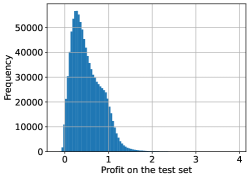
Figure 1. The histogram shows the distribution of the net profit $\mathcal{I}_{S_{i,j}}(K_{i},a_{i},h_{i})-f(\pi_{i},a_{i},h_{i})$ for $i=1,\dots,5000$, $j=1,\dots,200$ of the strategy trained as described in Section 3.1.1.

3.1.2. Backtesting with historical option prices

We backtest the strategy trained in Section 3.1.1 on the stocks of Apple, Alphabet, Microsoft, Google, and Meta. To this end, we consider for each of the companies call options with maturity $24$ March $2023$ for ten different strikes.

The bid and ask prices of these call options and the underlying securities were observed on $33$ trading days ranging from $2$ February $2023$ until $22$ March $2023$.

We apply the strategy trained in Section 3.1.1 to the prices observed on each of the $33$ trading days and evaluate it on the realized values of the $5$ underlying securities at maturity. In Table 2 and Figure 2 we summarize the net profits of the $33$ strategies. Note that to apply the trained neural network from Section 3.1.1, we first scale all the financial instruments such that the spot values of the underlying securities equal 1, as described in Section 3.1.1. Then, after applying the strategies to the scaled inputs, we rescale the values of the involved quantities back to unnormalized values, and we report in Table 2 and Figure 2 the net profits for both cases: after rescaling the values of the underlying securities, options, and strikes to unnormalized values, as well as without scaling back. The results of the backtesting study reveal that even though the neural network from Section 3.1.1 was trained on data extracted at a different day ($25$ April $2025$) involving call options with a different maturity written on other assets, the resultant strategy still allows to trade profitably in the majority of cases, showcasing the robustness of our algorithm.

	unscaled	scaled
count	33	33
mean	5.855233	0.063460
std	9.706270	0.089347
min	-4.225227	-0.017063
25%	-1.475227	-0.007025
50%	1.535172	0.021668
75%	13.032318	0.093558
max	32.687988	0.318201

Table 2. In the setting of Section 3.1.2, the table shows the summary statistics of the net profit $\mathcal{I}_{S_{T}}(K_{i},a_{i},h_{i})-f(\pi_{i},a_{i},h_{i})$ for $i=1,\dots,33$, where here $S_{T}\in\mathbb{R}^{5}$ refers to the observed realization of the $5$ underlying securities at maturity $T=$ $24$ March $2023$. To apply the trained neural network we first scale the values such that the spot prices of the underlying assets equal 1. The left column shows the values after scaling the values back, whereas the right column shows the statistics directly after applying the neural network to the scaled data.

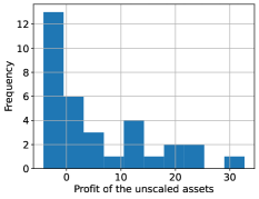
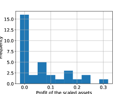
Figure 2. In the setting of Section 3.1.2, the histogram depicts the net profits $\mathcal{I}_{S_{T}}(K_{i},a_{i},h_{i})-f(\pi_{i},a_{i},h_{i})$ for $i=1,\dots,33$, where here $S_{T}\in\mathbb{R}^{5}$ refers to the observed realization of the $5$ underlying securities at maturity $T=$ $24$ March $2023$.

4. Approximation of optimal solutions of general convex semi-infinite programs by neural networks

In this section we show for a certain class of convex semi-infinite optimization problems (CSIP) that each of them can be approximately solved by a single neural networks. More precisely, for every prescribed accuracy $\varepsilon>0$ we show that there exists a single neural network which outputs a feasible solution which is $\varepsilon$-optimal. This class of convex semi-infinite problems covers the setting of static arbitrage detection introduced in Section 2 as special case. We leave further applications for future research.

4.1. Setting

Let $\underline{a}\in\mathbb{R}$, let $\mathbb{K}_{x}\subset\mathbb{R}^{n_{x}}$ be compact for some $n_{x}\in\mathbb{N}$, and let $\mathbb{K}_{y}\subset\mathbb{R}^{n_{y}}$ be compact and convex for some $n_{y}\in\mathbb{N}$.

We consider some function

$$f:\mathbb{K}_{x}\times[\underline{a},\infty)\times\mathbb{K}_{y}\ni(x,a,y)\mapsto f(x,a,y)\in\mathbb{R},$$

which we aim to minimize under suitable constraints. To define these constraints we consider some (possibly uncountable infinite) index set $\mathcal{S}$ as well as for all $s\in\mathcal{S}$ a function

$$\mathbb{K}_{x}\times[\underline{a},\infty)\times\mathbb{K}_{y}\ni(x,a,y)\mapsto\mathcal{I}_{s}(x,a,y)\in\mathbb{R}.$$

Further, let $\mathbb{K}_{x}\ni x\twoheadrightarrow\Gamma(X)\subseteq[\underline{a},\infty)\times\mathbb{K}_{y}$ be the correspondence defined by

$$\Gamma(x):=\left\{(a,y)\in[\underline{a},\infty)\times\mathbb{K}_{y}\leavevmode\nobreak\ \middle|\leavevmode\nobreak\ -\mathcal{I}_{s}(x,a,y)\leq 0\text{ for all }s\in\mathcal{S}\right\},$$

that defines the set of feasible elements from $[\underline{a},\infty)\times\mathbb{K}_{y}$. To define our optimization problem, we now consider the function $\mathbb{K}_{x}\ni x\mapsto V(x)\in\mathbb{R}$ defined by

(4.1) $$V(x):=\inf_{(a,y)\in\Gamma(x)}f(x,a,y).$$

We impose the following assumptions on the above defined quantities.

Assumption 4.1 (Assumptions on $f$).

• There exists some $L_{f}\geq 1$ such that the function $[\underline{a},\infty)\times\mathbb{K}_{y}\ni(a,y)\mapsto f(x,a,y)$ is $L_{f}$-Lipschitz continuous for all $x\in\mathbb{K}_{x}$.

• The function $\mathbb{K}_{x}\times[\underline{a},\infty)\times\mathbb{K}_{y}\ni(x,a,y)\mapsto f(x,a,y)$ is continuous.

• The function $[\underline{a},\infty)\times\mathbb{K}_{y}\ni(a,y)\mapsto f(x,a,y)$ is convex for all $x\in\mathbb{K}_{x}$.

• The function $[\underline{a},\infty)\ni a\mapsto f(x,a,y)$ is increasing for all $x\in\mathbb{K}_{x}$, $y\in\mathbb{K}_{y}$.

• We have that

  $$\mathcal{L}_{a,f}:=\inf_{x\in\mathbb{K}_{x},y\in\mathbb{K}_{y}\atop a_{1},a_{2}\in[\underline{a},\infty),a_{1}\neq a_{2}}\frac{|f(x,a_{1},y)-f(x,a_{2},y)|}{|a_{1}-a_{2}|}>0.$$

Assumption 4.2 (Assumptions on $\mathcal{I}_{s}$).

• There exists some ${L}_{\mathcal{I}}\geq 1$ such that $\mathbb{K}_{x}\times[\underline{a},\infty)\times\mathbb{K}_{y}\ni(x,a,y)\mapsto\mathcal{I}_{s}(x,a,y)$ is ${L}_{\mathcal{I}}$-Lipschitz continuous for all $s\in\mathcal{S}$.

• The function $[\underline{a},\infty)\times\mathbb{K}_{y}\ni(a,y)\mapsto\mathcal{I}_{s}(x,a,y)$ is concave for all $x\in\mathbb{K}_{x},s\in\mathcal{S}$.

• The function $[\underline{a},\infty)\ni a\mapsto\mathcal{I}_{s}(x,a,y)$ is increasing for all $x\in\mathbb{K}_{x},y\in\mathbb{K}_{y},s\in\mathcal{S}$.

• We have that

  $$\mathcal{L}_{a,\mathcal{I}}:=\inf_{s\in\mathcal{S}}\inf_{x\in\mathbb{K}_{x},\atop y\in\mathbb{K}_{y}}\inf_{a_{1}\neq a_{2},\atop a_{1},a_{2}\in[\underline{a},\infty)}\frac{\left|\mathcal{I}_{s}(x,a_{1},y)-\mathcal{I}_{s}(x,a_{2},y)\right|}{|a_{1}-a_{2}|}>0.$$

• We have that

  $$\inf_{s\in\mathcal{S},\atop x\in\mathbb{K}_{x},y\in\mathbb{K}_{y}}\mathcal{I}_{s}(x,\underline{a},y)>-\infty.$$

Assumption 4.3 (Assumptions on $\mathbb{K}_{y}$).

There exists $0<r<1$ and $L_{r}\geq 1$ such that for all $0<\delta<r$ there exists some closed and convex set $C_{y,\delta}\subset\mathbb{K}_{y}$ such that for all $y^{\prime}\in C_{y,\delta}$, $y\in\mathbb{R}^{n_{y}}$ we have

$$\|y^{\prime}-y\|\leq\delta\Rightarrow y\in\mathbb{K}_{y},$$

and

$$\max_{y\in\mathbb{K}_{y}}\min_{y^{\prime}\in C_{y,\delta}}\left\{\|y-y^{\prime}\|\right\}\leq L_{r}\delta.$$

Remark 4.4 (On the assumptions).

• Let

  (4.2) $$\overline{a}^{\operatorname{UB}}:=\underline{a}+\frac{1}{\mathcal{L}_{a,\mathcal{I}}}\left|\inf_{s\in\mathcal{S},\atop x\in\mathbb{K}_{x},y\in\mathbb{K}_{y}}\mathcal{I}_{s}(x,\underline{a},y)\right|\in[\underline{a},\infty)$$

  Then, we have $\mathcal{I}_{s}(x,\overline{a}^{\operatorname{UB}},y)\geq 0$ for all $x\in\mathbb{K}_{x}$, $y\in\mathbb{K}_{y}$, $s\in\mathcal{S}$. In particular, $\Gamma(x)\neq\emptyset$ for all $x\in\mathbb{K}_{x}$. Indeed, by using the definition of $\overline{a}^{\operatorname{UB}}$ and $\mathcal{L}_{a,\mathcal{I}}$ together with Assumption 4.2 (v) we have for all $x\in\mathbb{K}_{x}$, $y\in\mathbb{K}_{y}$, $s\in\mathcal{S}$ that

  $$\mathcal{I}_{s}(x,\overline{a}^{\operatorname{UB}},y) =\mathcal{I}_{s}(x,\overline{a}^{\operatorname{UB}},y)-\mathcal{I}_{s}(x,\underline{a},y)+\mathcal{I}_{s}(x,\underline{a},y)$$

  $$\geq\mathcal{L}_{a,\mathcal{I}}\cdot\overline{a}^{\operatorname{UB}}-\mathcal{L}_{a,\mathcal{I}}\cdot\underline{a}+\inf_{s\in\mathcal{S},\atop x\in\mathbb{K}_{x},y\in\mathbb{K}_{y}}\mathcal{I}_{s}(x,\underline{a},y)$$

  $$=\mathcal{L}_{a,\mathcal{I}}\cdot\left(\underline{a}+\frac{1}{\mathcal{L}_{a,\mathcal{I}}}\cdot\left|\inf_{s\in\mathcal{S},\atop x\in\mathbb{K}_{x},y\in\mathbb{K}_{y}}\mathcal{I}_{s}(x,\underline{a},y)\right|\right)-\mathcal{L}_{a,\mathcal{I}}\cdot\underline{a}+\inf_{s\in\mathcal{S},\atop x\in\mathbb{K}_{x},y\in\mathbb{K}_{y}}\mathcal{I}_{s}(x,\underline{a},y)\geq 0.$$

• Assumption 4.1 (ii) and  (iv), and the assumption that $\mathbb{K}_{x}$ and $\mathbb{K}_{y}$ are compact ensure together with Remark 4.4 (i) that $V(x)\in\mathbb{R}$ for all $x\in\mathbb{K}_{x}$. Indeed, for any $x\in\mathbb{K}_{x}$ and $(a,y)\in\Gamma(x)$, we have $f(x,a,y)\geq f(x,\underline{a},y)\geq\inf_{x\in\mathbb{K}_{x},y\in\mathbb{K}_{y}}f(x,\underline{a},y)>-\infty$.

• Assumption 4.1 (iv) and  (v) ensure that the function $f$ is strictly increasing in $a\in[\underline{a},\infty)$ uniformly in $x\in\mathbb{K}_{x}$, $y\in\mathbb{K}_{y}$. Analogously, Assumption 4.2 (iii) and  (iv) ensure that the function $\mathcal{I}$ is strictly increasing in $a\in[\underline{a},\infty)$ uniformly in $x\in\mathbb{K}_{x}$, $y\in\mathbb{K}_{y}$, $s\in\mathcal{S}$.

• Note that Assumption 4.3 roughly speaking means that the geometry of $\mathbb{K}_{y}\subseteq\mathbb{R}^{n_{y}}$ is similar to a box. Indeed, if $\mathbb{K}_{y}=\times_{i=1}^{n_{y}}[l_{i},u_{i}]$ for some $-\infty<\l_{i}<u_{i}<\infty$, $i=1,\dots,n_{y}$, then one can choose $0<r<\min_{i}(\frac{u_{i}-l_{i}}{2})>0$, $C_{y,\delta}:=\times_{i=1}^{n_{y}}[l_{i}+\delta,u_{i}-\delta]\subseteq\mathbb{K}_{y}$, and $L_{r}:=\sqrt{n_{y}}$.

Our main result of this section establishes the existence of a single neural network such that for any input $x\in\mathbb{K}_{x}$ defining the (CSIP) in (4.1) the neural network outputs a feasible solution which is $\varepsilon$-optimal.

Theorem 4.5 (Single neural network provides corresponding feasible $\varepsilon$-optimizer for class of (CSIP)).

Let Assumptions 4.1, 4.2, and 4.3 hold true. Then, for all $\varepsilon>0$ there exists a neural network $\mathcal{N}\mathcal{N}\in\mathfrak{N}_{n_{x},1+n_{y}}$ such that

• $\mathcal{N}\mathcal{N}(x):=\left(\mathcal{N}\mathcal{N}_{a}(x),\mathcal{N}\mathcal{N}_{y}(x)\right)\in\Gamma(x)$ for all $x\in\mathbb{K}_{x}$,

• $f\left(x,\mathcal{N}\mathcal{N}_{a}(x),\mathcal{N}\mathcal{N}_{y}(x)\right)-V(x)\leq\varepsilon$ for all $x\in\mathbb{K}_{x}$.

The proof of Theorem 4.5 is provided in the next section.

5. Proofs and Auxiliary Results

In this section, we present the proofs of the main results from Section 2 and  4.

5.1. Proofs of Section 2

The proof of Proposition 2.7 consists of verifying that the optimization problem (2.4) is included in the general (CSIP) introduced in Section 4. Then, applying Proposition 2.7 together with the universal approximation property of neural networks allows to conclude Theorem 2.5 and Theorem 2.6.

Proof of Proposition 2.7.

We verify that the conditions imposed in Theorem 4.5 are satisfied under Assumption 2.3 with $x\leftarrow(K,\pi)$, $a\leftarrow a$, $y\leftarrow h$, $V\leftarrow V$ in the notation of Theorem 4.5. To that end, note that Assumption 4.1 holds with $\mathcal{L}_{a,f}=1$, and $L_{f}=\max\{1,\leavevmode\nobreak\ \overline{\pi}\}\sqrt{1+2N}$. Moreover, note that for all $x\in\mathbb{K}_{x}$, $(a,0)\in\left([\underline{a},\infty)\cap[0,\infty)\right)\times[0,\overline{H}]^{2N}$ satisfies $\mathcal{I}_{S}(x,a,0)\geq 0$ for all $S\in\mathcal{S}$. Hence, Assumption 4.2 holds with $\mathcal{L}_{a,\mathcal{I}}=1$ and $L_{\mathcal{I}}=\max\{1,\leavevmode\nobreak\ 2\overline{H}L_{\Psi},\leavevmode\nobreak\ C_{\Psi}\}\sqrt{3N+1}$. Furthermore, for any $0<r<1$ and any $0<\delta<1$, Assumption 4.3 is satisfied with $C_{y,\delta}=[\delta,\overline{H}-\delta]^{2N}$ and $L_{r}=\sqrt{2N}$. Therefore, the result follows by Theorem 4.5.

∎

Proof of Theorem 2.5.

Let $(K,\pi)\in[0,\overline{K}]^{N}\times[0,\overline{H}]^{2N}$. Assume first there exists model-free arbitrage, i.e., we have $V(K,\pi)<0$. Then, we choose $\varepsilon\in\mathbb{R}$ with $0<\varepsilon<-V(K,\pi)$ and obtain with Proposition 2.7 the existence of a neural network $\mathcal{N}\mathcal{N}=(\mathcal{N}\mathcal{N}_{a},\mathcal{N}\mathcal{N}_{h})\in\mathfrak{N}_{3N,1+2N}$ with $\mathcal{N}\mathcal{N}(K,\pi)\in\Gamma(K)$ and with $f\left(\pi,\mathcal{N}\mathcal{N}_{a}(K,\pi),\mathcal{N}\mathcal{N}_{h}(K,\pi)\right)-V(K,\pi)\leq\varepsilon$ which implies

$$f\left(\pi,\mathcal{N}\mathcal{N}_{a}(K,\pi),\mathcal{N}\mathcal{N}_{h}(K,\pi)\right)\leq\varepsilon+V(K,\pi)<-V(K,\pi)+V(K,\pi)=0.$$

Conversely, if conditions (i) and (ii) hold, then the output of the neural network constitutes a model-free arbitrage opportunity. ∎

Proof of Theorem 2.6.

Let $\varepsilon>0$. By Proposition 2.7, there exists a neural network $\mathcal{N}\mathcal{N}\in\mathfrak{N}_{3N,1+2N}$ such that for every $(K,\pi)\in[0,\overline{K}]^{N}\times[0,\overline{\pi}]^{2N}$

$$\mathcal{N}\mathcal{N}(K,\pi):=\left(\mathcal{N}\mathcal{N}_{a}(K,\pi),\mathcal{N}\mathcal{N}_{h}(K,\pi)\right)\in\Gamma(K)$$

and $$f\left(\pi,\mathcal{N}\mathcal{N}_{a}(K,\pi),\mathcal{N}\mathcal{N}_{h}(K,\pi)\right)-V(K,\pi)\leq\varepsilon-\delta.$$

Moreover, for every $(K,\pi)\in[0,\overline{K}]^{N}\times[0,\overline{\pi}]^{2N}$, if the market with respect to $(K,\pi)$ admits model-free static arbitrage of magnitude $\varepsilon$, then by definition $V(K,\pi)\leq-\varepsilon$. This implies that $\mathcal{N}\mathcal{N}(K,\pi):=\left(\mathcal{N}\mathcal{N}_{a}(K,\pi),\mathcal{N}\mathcal{N}_{h}(K,\pi)\right)$ provides a model-free static arbitrage strategy of magnitude $\delta$.

If the market with respect to $(K,\pi)$ admits no model-free static arbitrage, then $V(K,\pi)=0$ and hence

$$f\left(\pi,\mathcal{N}\mathcal{N}_{a}(K,\pi),\mathcal{N}\mathcal{N}_{h}(K,\pi)\right)\leq V(K,\pi)+\varepsilon-\delta=\varepsilon-\delta.$$

∎

It remains to prove Theorem 4.5, which is our main technical result. Its proof is provided in the next subsection.

5.2. Proofs of Section 4

The main idea of the proof of Theorem 4.5 is to show that the correspondence of feasible $\varepsilon$-optimizers of the convex semi-infinite program (CSIP) defined in (4.1), as a function of the input $x\in\mathbb{K}_{x}$ of the (CSIP), is non-empty, convex, closed, and lower hemicontinuous, where the major difficulty lies in the establishment of the lower hemicontinuity. This then allows us to apply Michael’s continuous selection theorem (michael), which together with the universal approximation property of neural networks leads to the existence of a single neural network which for any input $x\in\mathbb{K}_{x}$ defining the (CSIP) in (4.1) outputs a feasible solution which is $\varepsilon$-optimal. We highlight that no strict-convexity of the map $(a,y)\mapsto f(x,a,y)$ for any fixed $x$ is assumed in (4.1), hence one cannot expect uniqueness of optimizers for the (CSIP), which in turn means that one cannot expect to have lower hemicontinuity of the correspondence of feasible true optimizers of the (CSIP) in (4.1).

5.2.1. Auxiliary Results

Before reporting the proof of Theorem 4.5, we establish several auxiliary results which are necessary for the proof of the main result from Theorem 4.5.

For all of the auxiliary results from Section 5.2.1 we assume the validity of Assumption 4.1, Assumption 4.2 and Assumption 4.3. Moreover, from now on, we define the following quantity

(5.1) $$\overline{a}^{\operatorname{UB}}:=\underline{a}+\frac{1}{\mathcal{L}_{a,\mathcal{I}}}\left|\inf_{s\in\mathcal{S},\atop x\in\mathbb{K}_{x},y\in\mathbb{K}_{y}}\mathcal{I}_{s}(x,\underline{a},y)\right|\in[\underline{a},\infty).$$

Lemma 5.1.

• Let $a\in[\underline{a},\infty)$ such that $a\geq\overline{a}^{\operatorname{UB}}$. Then, we have that $\mathcal{I}_{s}(x,a,y)\geq 0$ for all $x\in\mathbb{K}_{x}$, $y\in\mathbb{K}_{y}$, $s\in\mathcal{S}$.

• Let $a\in[\underline{a},\infty)$ such that $a\geq\overline{a}^{\operatorname{UB}}+\frac{1}{\mathcal{L}_{a,f}}$. Then, for all $x\in\mathbb{K}_{x}$ and for all $y\in\mathbb{K}_{y}$ we have $f(x,a,y)-V(x)\geq 1$.

Proof.

• Let $a\in[\underline{a},\overline{a}]$ such that $a\geq\overline{a}^{\operatorname{UB}}$. Further, let $x\in\mathbb{K}_{x}$, $y\in\mathbb{K}_{y}$, $s\in\mathcal{S}$. Then, we have by the monotonicity of $\mathcal{I}_{s}$ on $[\underline{a},\overline{a}]$ (stated in Assumption 4.2 (iii)) that

  (5.2) $$\mathcal{I}_{s}(x,a,y)\geq\mathcal{I}_{s}(x,\overline{a}^{\operatorname{UB}},y)=\mathcal{I}_{s}(x,\overline{a}^{\operatorname{UB}},y)-\mathcal{I}_{s}(x,\underline{a},y)+\mathcal{I}_{s}(x,\underline{a},y).$$

  By using the above inequality (5.2), Assumption 4.2 (iv), and the definition of $\overline{a}^{\operatorname{UB}}$ we then have

  $$\mathcal{I}_{s}(x,a,y) \geq\mathcal{L}_{a,\mathcal{I}}\cdot\left(\overline{a}^{\operatorname{UB}}-\underline{a}\right)+\inf_{s\in\mathcal{S},\atop x\in\mathbb{K}_{x},y\in\mathbb{K}_{y}}\mathcal{I}_{s}(x,\underline{a},y)$$

  $$=\mathcal{L}_{a,\mathcal{I}}\cdot\overline{a}^{\operatorname{UB}}-\mathcal{L}_{a,\mathcal{I}}\cdot\underline{a}+\inf_{s\in\mathcal{S},\atop x\in\mathbb{K}_{x},y\in\mathbb{K}_{y}}\mathcal{I}_{s}(x,\underline{a},y)$$

  $$=\mathcal{L}_{a,\mathcal{I}}\cdot\left(\underline{a}+\frac{1}{\mathcal{L}_{a,\mathcal{I}}}\left|\inf_{s\in\mathcal{S},\atop x\in\mathbb{K}_{x},y\in\mathbb{K}_{y}}\mathcal{I}_{s}(x,\underline{a},y)\right|\right)-\mathcal{L}_{a,\mathcal{I}}\cdot\underline{a}+\inf_{s\in\mathcal{S},\atop x\in\mathbb{K}_{x},y\in\mathbb{K}_{y}}\mathcal{I}_{s}(x,\underline{a},y)$$

  $$=\left|\inf_{s\in\mathcal{S},\atop x\in\mathbb{K}_{x},y\in\mathbb{K}_{y}}\mathcal{I}_{s}(x,\underline{a},y)\right|+\inf_{s\in\mathcal{S},\atop x\in\mathbb{K}_{x},y\in\mathbb{K}_{y}}\mathcal{I}_{s}(x,\underline{a},y)\geq 0.$$

• First note that, by the assertion from (i), we have $(\overline{a}^{\operatorname{UB}},y)\in\Gamma(x)$ for all $y\in\mathbb{K}_{y}$ and hence

  (5.3) $$f(x,\overline{a}^{\operatorname{UB}},y)\geq V(x)\text{ for all }x\in\mathbb{K}_{x},\leavevmode\nobreak\ y\in\mathbb{K}_{y}.$$

  Then, as by assumption $a\geq\overline{a}^{\operatorname{UB}}+\frac{1}{\mathcal{L}_{a,f}}$, we have for all $x\in\mathbb{K}_{x}$ and for all $y\in\mathbb{K}_{y}$ by Assumption 4.1 (iv), by Assumption 4.1 (v), and by (5.3), that

  $$f(x,a,y)-V(x) =f(x,a,y)-f(x,\overline{a}^{\operatorname{UB}},y)+f(x,\overline{a}^{\operatorname{UB}},y)-V(x)$$

  $$\geq\mathcal{L}_{a,f}\cdot(a-\overline{a}^{\operatorname{UB}})+f(x,\overline{a}^{\operatorname{UB}},y)-V(x)$$

  $$\geq\mathcal{L}_{a,f}\cdot(a-\overline{a}^{\operatorname{UB}})\geq 1.$$

∎

From now on, let

(5.4) $$\overline{a}:=\overline{a}^{\operatorname{UB}}+\frac{1}{\mathcal{L}_{a,f}}+2,$$

where $\overline{a}^{\operatorname{UB}}$ is defined in (5.1). Moreover, we define the correspondence

(5.5) $$X_{x}\ni x\twoheadrightarrow\Gamma_{\overline{a}}(x):=\left\{(a,y)\in\Gamma(x)\leavevmode\nobreak\ |\leavevmode\nobreak\ a\leq\overline{a}\right\}=\left\{(a,y)\in[\underline{a},\overline{a}]\times\mathbb{K}_{y}\leavevmode\nobreak\ |\leavevmode\nobreak\ \mathcal{I}_{s}(x,a,y)\geq 0\text{ for all }s\in\mathcal{S}\right\}.$$

Lemma 5.2.

Let $\overline{a}$ be defined in (5.4). Moreover, let $\mathbb{K}_{x}\ni x\mapsto\Gamma_{\overline{a}}(x)$ be defined in (5.5). Then, for all $x\in\mathbb{K}_{x}$, $\Gamma_{\overline{a}}(x)$ is nonempty, and for all $x\in\mathbb{K}_{x}$

$$V_{\overline{a}}(x):=\inf_{(a,y)\in\Gamma_{\overline{a}}(x)}f(x,a,y)=\inf_{(a,y)\in\Gamma(x)}f(x,a,y)=V(x).$$

Proof.

By Remark 4.4 (i) we see that $\Gamma_{\overline{a}}(x)\neq\emptyset$ for all $x\in\mathbb{K}_{x}$. Moreover, as $\Gamma_{\overline{a}}(x)\subseteq\Gamma(x)$, we have $V_{\overline{a}}(x)\geq V(x)$ for every $x\in\mathbb{K}_{x}$. To see that $V_{\overline{a}}(x)\leq V(x)$ for every $x\in\mathbb{K}_{x}$, fix any $x\in\mathbb{K}_{x}$ and let $(a,y)\in\Gamma(x)$. By Remark 4.4 (i), we have $(\overline{a}^{\operatorname{UB}},y)\in\Gamma_{\overline{a}}(x)$. Hence, $f(x,a,y)\geq f(x,\min\{a,\overline{a}^{\operatorname{UB}}\},y)\geq\inf_{(\widetilde{a},\widetilde{y})\in\Gamma_{\overline{a}}(x)}f(x,\widetilde{a},\widetilde{y})$. Since $(a,y)\in\Gamma(x)$ was arbitrary we obtain the desired result. ∎

Lemma 5.3.

The map $\mathbb{K}_{x}\ni x\twoheadrightarrow\Gamma_{\overline{a}}(x)$ defined in (5.5) is a non-empty, compact-valued, convex-valued, and continuous correspondence.

Proof.

The non-emptiness follows from Remark 4.4.

Let $x\in\mathbb{K}_{x}$. Consider a sequence $(a^{(n)},y^{(n)})_{n\in\mathbb{N}}\subseteq\Gamma_{\overline{a}}(x)$. Then, by the compactness of $[\underline{a},\overline{a}]\times\mathbb{K}_{y}$, there exists a subsequence $(a^{(n_{k})},y^{(n_{k})})_{k\in\mathbb{N}}\subseteq\Gamma_{\overline{a}}(x)$ such that $(a^{(n_{k})},y^{(n_{k})})\rightarrow(a,y)$ as $k\rightarrow\infty$ for some $(a,y)\in[\underline{a},\overline{a}]\times\mathbb{K}_{y}$. The continuity of $[\underline{a},\overline{a}]\times\mathbb{K}_{y}\ni(a,y)\mapsto\mathcal{I}_{s}(x,a,y)$, which is ensured by Assumption 4.2 (i), then implies that $0\leq\lim_{k\rightarrow\infty}\mathcal{I}_{s}(x,a^{(n_{k})},y^{(n_{k})})=\mathcal{I}_{s}(x,a,y)$. Hence, $\Gamma_{\overline{a}}(x)$ is compact.

Let $x\in\mathbb{K}_{x}$, and let $(a,y),\leavevmode\nobreak\ (a^{\prime},y^{\prime})\in\Gamma_{\overline{a}}(x)$. Then, it follows for all $t\in[0,1]$ by Assumption 4.2 (ii) that

$$\mathcal{I}_{s}\left(x,\leavevmode\nobreak\ t\cdot a+(1-t)a^{\prime},\leavevmode\nobreak\ ty+(1-t)\cdot y^{\prime}\right)\geq t\cdot\mathcal{I}_{s}(x,a,y)+(1-t)\cdot\mathcal{I}_{s}(x,a^{\prime},y^{\prime})\geq 0\text{ for all }s\in\mathcal{S}.$$

Hence, the convexity of (5.5) follows.

It remains to show the continuity, i.e., that the map from (5.5) is lower hemicontinuous and upper hemicontinuous.

Let $(x^{(n)})_{n\in\mathbb{N}}\subseteq\mathbb{K}_{x}$ with $\lim_{n\rightarrow\infty}x^{(n)}=x\in\mathbb{K}_{x}$ and let $(a,y)\in\Gamma_{\overline{a}}(x)\subseteq[\underline{a},\overline{a}]\times\mathbb{K}_{y}$. To show the lower-hemicontinuity, according to the characterization provided, e.g., in (Aliprantis, Theorem 17.21), we need to prove the existence of a subsequence $(x^{(n_{k})})_{k\in\mathbb{N}}$ and elements $(a^{(k)},y^{(k)})\in\Gamma(x^{(n_{k})})$ for each $k\in\mathbb{N}$ with $\lim_{k\rightarrow\infty}(a^{(k)},y^{(k)})=(a,y)$.

First assume that $a\leq\overline{a}^{\operatorname{UB}}$. Since $\lim_{n\rightarrow\infty}x^{(n)}=x$, there exists, by definition of $\overline{a}$, some $n_{0}\in\mathbb{N}$ such that for all $n\geq n_{0}$ we have

(5.6) $$a^{(n)}:=a+\frac{{L}_{\mathcal{I}}}{\mathcal{L}_{a,\mathcal{I}}}\cdot\left\|x^{(n)}-x\right\|\leq\overline{a}.$$

Since by Assumption 4.2 (iii) the map $[\underline{a},\overline{a}]\ni a\mapsto\mathcal{I}_{s}(x,a,y)$ is monotone for all $x\in\mathbb{K}_{x},y\in\mathbb{K}_{y},s\in\mathcal{S}$, with Assumption 4.2  (iv), and with the Lipschitz-property of $\mathcal{I}_{s}$ from Assumption 4.2 (i), we have for all $s\in\mathcal{S}$ and for all $n\in\mathbb{N}$ that

$$\mathcal{I}_{s}\left(x^{(n)},\leavevmode\nobreak\ a^{(n)},\leavevmode\nobreak\ y\right) =\mathcal{I}_{s}\left(x^{(n)},\leavevmode\nobreak\ a,\leavevmode\nobreak\ y\right)-\mathcal{I}_{s}\left(x^{(n)},\leavevmode\nobreak\ a,\leavevmode\nobreak\ y\right)+\mathcal{I}_{s}\left(x^{(n)},\leavevmode\nobreak\ a+\frac{{L}_{\mathcal{I}}}{\mathcal{L}_{a,\mathcal{I}}}\cdot\left\|x^{(n)}-x\right\|,\leavevmode\nobreak\ y\right)$$

$$\geq\mathcal{I}_{s}\left(x^{(n)},\leavevmode\nobreak\ a,\leavevmode\nobreak\ y\right)+\mathcal{L}_{a,\mathcal{I}}\cdot\frac{{L}_{\mathcal{I}}}{\mathcal{L}_{a,\mathcal{I}}}\cdot\left\|x^{(n)}-x\right\|$$

$$\geq\mathcal{I}_{s}\left(x^{(n)},\leavevmode\nobreak\ a,\leavevmode\nobreak\ y\right)-\mathcal{I}_{s}\left(x^{(n)},\leavevmode\nobreak\ a,\leavevmode\nobreak\ y\right)+\mathcal{I}_{s}\left(x,\leavevmode\nobreak\ a,\leavevmode\nobreak\ y\right)\geq 0,$$

where the last inequality follows since $(a,y)\in\Gamma_{\overline{a}}(x)$. Thus, we have $(a^{(n)},y)\in\Gamma_{\overline{a}}(x^{(n)})$ for all $n\geq n_{0}$ as well as by (5.6) that $\lim_{n\rightarrow\infty}(a^{(n)},y)=(a,y)$. Hence lower-hemicontinuity follows for the case $a\leq\overline{a}^{\operatorname{UB}}$.
Now we consider the case that $a>\overline{a}^{\operatorname{UB}}$. Note that in this case $\mathcal{I}_{s}(x,a,y)>0$ for all $s\in\mathcal{S}$ due to the strict monotonocity of $\mathcal{I}_{s}$ and by Remark 4.4 (i). Hence, by the continuity of $\mathcal{I}_{s}$, there exists some $n_{0}\in\mathbb{N}$ such that for all $n\geq n_{0}$ we have $\mathcal{I}_{s}(x^{(n)},a,y)>0$ implying that $(a,y)\in\Gamma_{\overline{a}}(x^{(n)})$ for all $n\geq n_{0}$. Thus, we conclude with (Aliprantis, Theorem 17.21) the lower hemicontinuity of the map from (5.5) also for the case $a>\overline{a}^{\operatorname{UB}}$.

It remains to show the upper hemicontinuity. To this end, let $(x^{(n)},a^{(n)},y^{(n)})\in\operatorname{Gr}\Gamma_{\overline{a}}$ with $\lim_{n\rightarrow}x^{(n)}=x$. We apply the characterization of upper hemicontinuity provided, e.g., in (Aliprantis, Theorem 17.20), and therefore we need to show the existence of a subsequence $(a^{(n_{k})},y^{(n_{k})})_{k\in\mathbb{N}}$ with $\lim_{k\rightarrow\infty}(a^{(n_{k})},y^{(n_{k})})=(a,y)\in\Gamma_{\overline{a}}(x)$.

As $(a^{(n)},y^{(n)})_{n\in\mathbb{N}}\subseteq[\underline{a},\overline{a}]\times\mathbb{K}_{y}$ is a sequence defined on a compact space, there exists a subsequence $(a^{(n_{k})},y^{(n_{k})})_{k\in\mathbb{N}}$ with $\lim_{k\rightarrow\infty}(a^{(n_{k})},y^{(n_{k})})=(a,y)\in[\underline{a},\overline{a}]\times\mathbb{K}_{y}$. Since $\mathcal{I}_{s}(x^{(n_{k})},a^{(n_{k})},y^{(n_{k})})\geq 0$ for all $k\in\mathbb{N}$ as $\left(x^{(n_{k})},a^{(n_{k})},y^{(n_{k})}\right)\in\operatorname{Gr}\Gamma_{\overline{a}}$, we obtain by the continuity of $\mathcal{I}_{s}$ that $\mathcal{I}_{s}(x,a,y)\geq 0$. This means $(a,y)\in\Gamma_{\overline{a}}(x)$. ∎

Lemma 5.4.

For all $\varepsilon\in(0,1)$ the correspondence

(5.7) $$\mathbb{K}_{x}\ni x\twoheadrightarrow\mathcal{M}_{\varepsilon}(x):=\left\{(a,y)\in\Gamma_{\overline{a}}(x)\leavevmode\nobreak\ \middle|\leavevmode\nobreak\ f(x,a,y)-V_{\overline{a}}(x)<\varepsilon\right\}$$

is non-empty, convex-valued, and lower hemicontinuous.

Proof.

Let $\varepsilon\in(0,1)$. The non-emptiness of $\mathcal{M}_{\varepsilon}(x)$ for each $x\in\mathbb{K}_{x}$ follows by definition and by Remark 4.4. To show the convexity of $\mathcal{M}_{\varepsilon}(x)$ for each $x\in\mathbb{K}_{x}$, fix any $x\in\mathbb{K}_{x}$ and let $(y,a),\leavevmode\nobreak\ (\widetilde{y},\widetilde{a})\in\mathcal{M}_{\varepsilon}(x)$ and $t\in[0,1]$. Then by Lemma 5.3 implying that $\Gamma_{\overline{a}}(x)$ is convex, we have $t\cdot(a,y)+(1-t)\cdot(\widetilde{y},\widetilde{a})\in\Gamma_{\overline{a}}(x)$. Moreover, by Assumption 4.1 (iii) ensuring that $[\underline{a},\overline{a}]\times\mathbb{K}_{y}\ni(a,y)\mapsto f(x,a,y)$ is convex, we have

$$f\left(x,t\cdot a+(1-t)\cdot\widetilde{a},t\cdot y+(1-t)\cdot\widetilde{y}\right)-V_{\overline{a}}(x)$$

$$\leq t\cdot\left(f\left(x,a,y\right)-V_{\overline{a}}(x)\right)+(1-t)\cdot\left(f\left(x,\widetilde{a},\widetilde{y}\right)-V_{\overline{a}}(x)\right)\leq t\cdot\varepsilon+(1-t)\cdot\varepsilon=\varepsilon,$$

from which we conclude the convexity of $\mathcal{M}_{\varepsilon}(x)$. To show the lower hemicontinuity of (5.7) let $(x^{(n)})_{n\in\mathbb{N}}\subseteq\mathbb{K}_{x}$ with $\lim_{n\rightarrow\infty}x^{(n)}=x\in\mathbb{K}_{x}$, and let $(a,y)\in\mathcal{M}_{\varepsilon}(x)$. We apply the characterization of lower hemicontinuity from (Aliprantis, Theorem 17.20) and therefore aim at showing that there exists a subsequence $(x^{(n_{k})})_{k\in\mathbb{N}}$ and elements $(a^{(k)},y^{(k)})\in\mathcal{M}_{\varepsilon}(x^{(n_{k})})$ for each $k\in\mathbb{N}$ such that $\lim_{k\rightarrow\infty}(a^{(k)},y^{(k)})=(a,y)$.

By Lemma 5.3 the correspondence $\mathbb{K}_{x}\ni x\twoheadrightarrow\Gamma_{\overline{a}}(x)$ is non-empty, compact-valued, continuous, and by Assumption 4.1 (ii), the map $\mathbb{K}_{x}\times[\underline{a},\overline{a}]\times\mathbb{K}_{y}\ni(x,a,y)\mapsto f(x,a,y)$ is continuous. Hence, Berge’s maximum theorem (see berge or (Aliprantis, Theorem 17.31)) is applicable.

We then obtain by Berge’s maximum theorem that the map

$$\mathbb{K}_{x}\ni x\mapsto V_{\overline{a}}(x):=\inf_{(a,y)\in\Gamma_{\overline{a}}(x)}f(x,a,y)$$

is continuous. Therefore, as $(a,y)\in\mathcal{M}_{\varepsilon}(x)$, and since both $f$ and $V_{\overline{a}}$ are continuous, there exists some $\gamma\in(0,1)$ such that for all $(x,^{\prime}a^{\prime},y^{\prime})$ with $(x,^{\prime}a^{\prime},y^{\prime})\in\mathcal{B}_{\gamma}(x,a,y)\subseteq\mathbb{K}_{x}\times[\underline{a},\overline{a}]\times\mathbb{K}_{y}$, it holds

(5.8) $$f(x^{\prime},a^{\prime},y^{\prime})-V_{\overline{a}}(x^{\prime})<\varepsilon.$$

Moreover, as $\lim_{n\rightarrow\infty}x^{(n)}=x$, there exist some $n_{0}\in\mathbb{N}$ such that for all $n\geq n_{0}$ we have

(5.9) $$\sqrt{\left\|x^{(n)}-x\right\|^{2}+\left(\frac{L_{\mathcal{I}}}{\mathcal{L}_{a,\mathcal{I}}}\left\|x^{(n)}-x\right\|\right)^{2}}\leq\gamma.$$

Moreover, since $(a,y)\in\mathcal{M}_{\varepsilon}(x)$ and $\varepsilon\in(0,1)$, we have by Lemma 5.1 (ii) that $a<\overline{a}^{\operatorname{UB}}+\tfrac{1}{\mathcal{L}_{a,f}}$. Hence, by (5.9) and by definition of $\overline{a}$ we have for all $n\geq n_{0}$ also that

(5.10) $$a+\frac{L_{\mathcal{I}}}{\mathcal{L}_{a,\mathcal{I}}}\left\|x^{(n)}-x\right\|\leq a+\gamma\leq\overline{a}.$$

Note also that for $n\geq n_{0}$ we have by Assumption 4.2 (iv) and Assumption 4.2 (i) for all $s\in\mathcal{S}$ the following inequality

(5.11) $$\mathcal{I}_{s}\left(x^{(n)},\leavevmode\nobreak\ a+\frac{L_{\mathcal{I}}}{\mathcal{L}_{a,\mathcal{I}}}\left\|x^{(n)}-x\right\|,\leavevmode\nobreak\ y\right) =\mathcal{I}_{s}\left(x^{(n)},\leavevmode\nobreak\ a+\frac{L_{\mathcal{I}}}{\mathcal{L}_{a,\mathcal{I}}}\left\|x^{(n)}-x\right\|,\leavevmode\nobreak\ y\right)-\mathcal{I}_{s}\left(x^{(n)},\leavevmode\nobreak\ a,\leavevmode\nobreak\ y\right)$$

$$\hskip 176.407pt+\mathcal{I}_{s}\left(x^{(n)},\leavevmode\nobreak\ a,\leavevmode\nobreak\ y\right)$$

$$\geq\mathcal{L}_{a,\mathcal{I}}\frac{L_{\mathcal{I}}}{\mathcal{L}_{a,\mathcal{I}}}\left\|x^{(n)}-x\right\|+\mathcal{I}_{s}\left(x^{(n)},\leavevmode\nobreak\ a,\leavevmode\nobreak\ y\right)$$

$$={L_{\mathcal{I}}}\left\|x^{(n)}-x\right\|+\mathcal{I}_{s}\left(x^{(n)},\leavevmode\nobreak\ a,\leavevmode\nobreak\ y\right)-\mathcal{I}_{s}\left(x,\leavevmode\nobreak\ a,\leavevmode\nobreak\ y\right)+\mathcal{I}_{s}\left(x,\leavevmode\nobreak\ a,\leavevmode\nobreak\ y\right)$$

$$\geq L_{\mathcal{I}}\left\|x^{(n)}-x\right\|-L_{\mathcal{I}}\left\|x^{(n)}-x\right\|+\mathcal{I}_{s}\left(x,\leavevmode\nobreak\ a,\leavevmode\nobreak\ y\right)\geq 0,$$

since $(a,y)\in\Gamma_{\overline{a}}(x)$. Hence, (5.10) and (5.11) together show that

(5.12) $$\left(a+\frac{L_{\mathcal{I}}}{\mathcal{L}_{a,\mathcal{I}}}\left\|x^{(n)}-x\right\|,\leavevmode\nobreak\ y\right)\in\Gamma_{\overline{a}}(x^{(n)})\text{ for all }n\geq n_{0}.$$

By (5.9) we have $\left(x^{(n)},a+\frac{L_{\mathcal{I}}}{\mathcal{L}_{a,\mathcal{I}}}\left\|x^{(n)}-x\right\|,\leavevmode\nobreak\ y\right)\in\mathcal{B}_{\gamma}(x,a,y)$ for all $n\geq n_{0}$. Thus, it follows with (5.8) and (5.12) that

$$\left(a+\frac{L_{\mathcal{I}}}{\mathcal{L}_{a,\mathcal{I}}}\left\|x^{(n)}-x\right\|,\leavevmode\nobreak\ y\right)\in\mathcal{M}_{\varepsilon}\left(x^{(n)}\right)\text{ for all }n\geq n_{0},$$

proving the lower hemicontinuity of (5.7), by applying the characterization of lower hemicontinuity from (Aliprantis, Theorem 17.20) to the subsequences $(x^{(n)})_{n\in\mathbb{N},\atop n\geq n_{0}}$ and $\left(a+\frac{L_{\mathcal{I}}}{\mathcal{L}_{a,\mathcal{I}}}\left\|x^{(n)}-x\right\|,\leavevmode\nobreak\ y\right)_{n\in\mathbb{N},\atop n\geq n_{0}}$. ∎

Corollary 5.5.

For all $\varepsilon\in(0,1)$ the correspondence

(5.13) $$\mathbb{K}_{x}\ni x\twoheadrightarrow\overline{\mathcal{M}_{\varepsilon}(x)}:=\operatorname{cl}\left(\mathcal{M}_{\varepsilon}(x)\right)$$

is nonempty, convex, closed, lower hemicontinuous, and satisfies

(5.14) $$\overline{\mathcal{M}_{\varepsilon}(x)}\subseteq\left\{(a,y)\in\Gamma_{\overline{a}}(x)\leavevmode\nobreak\ \middle|\leavevmode\nobreak\ f(x,a,y)-V_{\overline{a}}(x)\leq\varepsilon\right\}.$$

Proof.

The non-emptiness and convexity of the map defined in (5.13) both follow from Lemma 5.4. That the map is closed is a consequence of the definition of a closure of a set. The lower-hemicontinuity also follows from Lemma 5.4 and from (Aliprantis, Theorem 17.22 (1), p. 566) which ensures that the closure of a lower hemicontinuous map is again lower hemicontinuous. The relation (5.14) follows as the map $\mathbb{K}_{x}\times[\underline{a},\overline{a}]\times\mathbb{K}_{y}\ni(x,a,y)\mapsto f(x,a,y)$ is continuous by Assumption 4.1 (ii). ∎

Corollary 5.6.

For all $\varepsilon\in(0,1)$ there exists a continuous map $\mathbb{K}_{x}\ni x\mapsto\left(a^{*,\varepsilon}(x),\leavevmode\nobreak\ y^{*,\varepsilon}(x)\right)\in\Gamma_{\overline{a}}(x)$ satisfying both

• $a^{*,\varepsilon}(x)\leq\overline{a}^{\operatorname{UB}}+\frac{1}{\mathcal{L}_{a,f}}$ for all $x\in\mathbb{K}_{x}$,

• $f\left(x,\leavevmode\nobreak\ a^{*,\varepsilon}(x),\leavevmode\nobreak\ y^{*,\varepsilon}\right)-V_{\overline{a}}(x)\leq\varepsilon$.

Proof.

Corollary 5.5 ensures that the requirements for an application of the Michael selection theorem (see michael or (Aliprantis, Theorem 17.66)) are fulfilled. By the Michael selection theorem we then obtain a continuous selector $\mathbb{K}_{x}\ni x\mapsto\left(a^{*,\varepsilon}(x),\leavevmode\nobreak\ y^{*,\varepsilon}(x)\right)\in\operatorname{cl}\left(\mathcal{M}_{\varepsilon}(x)\right)\subseteq\Gamma_{\overline{a}}(x)$ implying, by definition of $\mathcal{M}_{\varepsilon}(x)$, that (ii) is fulfilled.

Assume now that (i) does not hold, i.e., that we have $a^{*,\varepsilon}(x)>\overline{a}^{\operatorname{UB}}+\frac{1}{\mathcal{L}_{a,f}}$. This, however, by Lemma 5.1 (ii), contradicts (ii), which concludes the proof. ∎

Now, for any $0<\delta<r$ recall the definition of the set $C_{y,\delta}\subseteq\mathbb{K}_{y}$ from Assumption 4.3.

Lemma 5.7.

For all $\delta\in(0,r)$, the map

$$\mathbb{K}_{x}\ni x\mapsto\big{(}{a_{\delta}}^{*,\varepsilon}(x),\leavevmode\nobreak\ {y_{\delta}}^{*,\varepsilon}(x)\big{)}:=\underset{(a,y)\in[\underline{a}+\delta,\overline{a}-\delta]\times C_{y,\delta}}{\operatorname{argmin}}\left\|(a,y)-\left(a^{*,\varepsilon}(x),y^{*,\varepsilon}(x)\right)\right\|^{2}$$

is continuous.

Proof.

Note that $(x,a,y)\mapsto\left\|(a,y)-\left(a^{*,\varepsilon}(x),y^{*,\varepsilon}(x)\right)\right\|^{2}$ is continuous by Corollary 5.6. Moreover, the single-valued map is well-defined as the projection of the point $\big{(}{a}^{*,\varepsilon}(x),\leavevmode\nobreak\ y^{*,\varepsilon}(x)\big{)}$ onto the compact, convex set $[\underline{a}+\delta,\overline{a}-\delta]\times C_{y,\delta}$. The continuity follows now by, e.g., Berge’s maximum theorem ((Aliprantis, Theorem 17.31)) and (Aliprantis, Lemma 17.6). ∎

5.2.2. Proof of Theorem 4.5

In Section 5.2.1 we have established all auxiliary results that allow us now to report the proof of Theorem 4.5.

Proof of Theorem 4.5.

Without loss of generality let $\varepsilon\in(0,1)$, else we substitute $\varepsilon$ by $\overline{\varepsilon}:=\frac{\varepsilon}{1+\varepsilon}$. By Corollary 5.6, for all $x\in\mathbb{K}_{x}$ there exists, by abuse of notation with $\varepsilon\leftarrow\varepsilon/2$ in the notation of Corollary 5.6, some continuous map $\mathbb{K}_{x}\ni x\mapsto\left(a^{*,\varepsilon}(x),\leavevmode\nobreak\ y^{*,\varepsilon}(x)\right)\in\Gamma_{\overline{a}}(x)$ satisfying for all $x\in\mathbb{K}_{x}$ that

(5.15) $$a^{*,\varepsilon}(x)\leq\overline{a}^{\operatorname{UB}}+\frac{1}{\mathcal{L}_{a,f}}$$

and such that

(5.16) $$f\left(x,\leavevmode\nobreak\ a^{*,\varepsilon}(x),\leavevmode\nobreak\ y^{*,\varepsilon}\right)-V_{\overline{a}}(x)\leq\varepsilon/2.$$

We recall $r\in(0,1)$ from Assumption 4.3 and define

(5.17) $$\delta_{0}:=\frac{\varepsilon\min\{\mathcal{L}_{a,\mathcal{I}},1\}}{8\max\left\{L_{\mathcal{I}},\mathcal{L}_{a,f}\right\}\sqrt{1+L_{r}^{2}}L_{f}}\cdot r\in(0,r).$$

Note that by definition of the projection from Lemma 5.7 with respect to $[\underline{a}-\delta_{0},\underline{a}+\delta_{0}]\times C_{y,\delta_{0}}$, and by Assumption 4.3 we have

(5.18) $$\left\|\left(x,a^{*,\varepsilon}(x),\leavevmode\nobreak\ y^{*,\varepsilon}(x)\right)-\left(x,a_{\delta_{0}}^{*,\varepsilon}(x),\leavevmode\nobreak\ y_{\delta_{0}}^{*,\varepsilon}(x)\right)\right\|\leq\sqrt{\delta_{0}^{2}+L_{r}^{2}\delta_{0}^{2}}=\delta_{0}\sqrt{1+L_{r}^{2}}\text{ for all }x\in\mathbb{K}_{x}.$$

Hence, for all $x\in\mathbb{K}_{x}$, by using the Lipschitz-continuity of $f$ from Assumption 4.1 (i), by (5.18), and by the definition of $\delta_{0}$ in (5.17), we have

(5.19) $$\left|f\left(x,a^{*,\varepsilon}(x),\leavevmode\nobreak\ y^{*,\varepsilon}(x)\right)-f\left(x,a_{\delta_{0}}^{*,\varepsilon}(x),\leavevmode\nobreak\ y_{\delta_{0}}^{*,\varepsilon}(x)\right)\right| \leq L_{f}\left\|\left(x,a^{*,\varepsilon}(x),\leavevmode\nobreak\ y^{*,\varepsilon}(x)\right)-\left(x,a_{\delta_{0}}^{*,\varepsilon}(x),\leavevmode\nobreak\ y_{\delta_{0}}^{*,\varepsilon}(x)\right)\right\|$$

$$\leq L_{f}\cdot\delta_{0}\sqrt{1+L_{r}^{2}}$$

$$=r\cdot\frac{L_{f}}{L_{f}}\frac{\sqrt{1+L_{r}^{2}}}{\sqrt{1+L_{r}^{2}}}\cdot\frac{\varepsilon\min\{\mathcal{L}_{a,\mathcal{I}},1\}}{8\max\left\{L_{\mathcal{I}},\mathcal{L}_{a,f}\right\}}\leq\frac{\varepsilon}{8}.$$

By Corollary 5.5, we have $(x,a^{*,\varepsilon}(x),y^{*,\varepsilon}(x))\in\Gamma_{\overline{a}}(x)$, and in particular, $\mathcal{I}_{s}(x,a^{*,\varepsilon}(x),y^{*,\varepsilon}(x))\geq 0$ for all $s\in\mathcal{S}$ and all $x\in\mathbb{K}_{x}$. This implies by the Lipschitz-continuity of $\mathcal{I}_{s}$ (Assumption 4.2 (i)), by using (5.18), and the definition of $\delta_{0}$, that

(5.20) $$\mathcal{I}_{s}(x,\leavevmode\nobreak\ a_{\delta_{0}}^{*,\varepsilon}(x),\leavevmode\nobreak\ y_{\delta_{0}}^{*,\varepsilon}(x)) =\mathcal{I}_{s}(x,\leavevmode\nobreak\ a_{\delta_{0}}^{*,\varepsilon}(x),\leavevmode\nobreak\ y_{\delta_{0}}^{*,\varepsilon}(x))-\mathcal{I}_{s}(x,\leavevmode\nobreak\ a^{*,\varepsilon}(x),\leavevmode\nobreak\ y^{*,\varepsilon}(x))+\mathcal{I}_{s}(x,\leavevmode\nobreak\ a^{*,\varepsilon}(x),\leavevmode\nobreak\ y^{*,\varepsilon}(x))$$

$$\geq-L_{\mathcal{I}}\left\|\left(x,a^{*,\varepsilon}(x),\leavevmode\nobreak\ y^{*,\varepsilon}(x)\right)-\left(x,a_{\delta_{0}}^{*,\varepsilon}(x),\leavevmode\nobreak\ y_{\delta_{0}}^{*,\varepsilon}(x)\right)\right\|$$

$$\geq-L_{\mathcal{I}}\delta_{0}\sqrt{1+L_{r}^{2}}$$

$$=-r\cdot\frac{\sqrt{1+L_{r}^{2}}}{\sqrt{1+L_{r}^{2}}}\cdot\frac{\min\{\mathcal{L}_{a,\mathcal{I}},1\}}{L_{f}}\cdot\frac{L_{\mathcal{I}}}{\max\left\{L_{\mathcal{I}},\mathcal{L}_{a,f}\right\}}\cdot\frac{\varepsilon}{8}\geq-\frac{\mathcal{L}_{a,\mathcal{I}}}{L_{f}}\frac{\varepsilon}{8}.$$

By the universal approximation theorem (Proposition 2.2) and Lemma 5.7 there exists a neural network $\widetilde{\mathcal{N}\mathcal{N}}:=\left(\widetilde{\mathcal{N}\mathcal{N}}_{a},\widetilde{\mathcal{N}\mathcal{N}}_{y}\right)\in\mathfrak{N}_{n_{x},1+n_{y}}$ such that

(5.21) $$\sup_{x\in\mathbb{K}_{x}}\left\|\left({a}_{\delta_{0}}^{*,\varepsilon}(x),\leavevmode\nobreak\ {y}_{\delta_{0}}^{*,\varepsilon}(x)\right)-\left(\widetilde{\mathcal{N}\mathcal{N}}_{a}(x),\widetilde{\mathcal{N}\mathcal{N}}_{y}(x)\right)\right\|<\delta_{0}.$$

Moreover, we have by (5.20) and (5.21) for all $x\in\mathbb{K}_{x}$, $s\in\mathcal{S}$ that

(5.22) $$\mathcal{I}_{s}(x,\widetilde{\mathcal{N}\mathcal{N}}_{a}(x),\widetilde{\mathcal{N}\mathcal{N}}_{y}(x)) =\mathcal{I}_{s}(x,\widetilde{\mathcal{N}\mathcal{N}}_{a}(x),\widetilde{\mathcal{N}\mathcal{N}}_{y}(x))-\mathcal{I}_{s}(x,{a}_{\delta_{0}}^{*,\varepsilon}(x),\leavevmode\nobreak\ {y}_{\delta_{0}}^{*,\varepsilon}(x))+\mathcal{I}_{s}(x,{a}_{\delta_{0}}^{*,\varepsilon}(x),\leavevmode\nobreak\ {y}_{\delta_{0}}^{*,\varepsilon}(x))$$

$$\geq-L_{\mathcal{I}}\delta_{0}+\mathcal{I}_{s}(x,{a}_{\delta_{0}}^{*,\varepsilon}(x),\leavevmode\nobreak\ {y}_{\delta_{0}}^{*,\varepsilon}(x))$$

$$\geq-L_{\mathcal{I}}\frac{\varepsilon\min\{\mathcal{L}_{a,\mathcal{I}},1\}}{8\max\left\{L_{\mathcal{I}},\mathcal{L}_{a,f}\right\}\sqrt{1+L_{r}^{2}}L_{f}}\cdot r-\frac{\mathcal{L}_{a,\mathcal{I}}}{L_{f}}\frac{\varepsilon}{8}$$

$$\geq-\frac{\mathcal{L}_{a,\mathcal{I}}}{L_{f}}\frac{\varepsilon}{8}-\frac{\mathcal{L}_{a,\mathcal{I}}}{L_{f}}\frac{\varepsilon}{8}=-\frac{\mathcal{L}_{a,\mathcal{I}}}{L_{f}}\frac{\varepsilon}{4}.$$

In addition, we have by (5.21) and Assumption 4.3 that $\left(\widetilde{\mathcal{N}\mathcal{N}}_{a}(x),\widetilde{\mathcal{N}\mathcal{N}}_{y}(x)\right)\in[\underline{a},\overline{a}]\times\mathbb{K}_{y}$ for all $x\in\mathbb{K}_{x}$. Furthermore, for all $x\in\mathbb{K}_{x}$

(5.23) $$\left|f\left(x,\widetilde{\mathcal{N}\mathcal{N}}_{a}(x),\widetilde{\mathcal{N}\mathcal{N}}_{y}(x)\right)-f\left(x,{a}_{\delta_{0}}^{*,\varepsilon}(x),\leavevmode\nobreak\ {y}_{\delta_{0}}^{*,\varepsilon}(x)\right)\right|\leq L_{f}\delta_{0}=r\cdot\frac{L_{f}}{L_{f}}\frac{\varepsilon\min\{\mathcal{L}_{a,\mathcal{I}},1\}}{8\max\left\{L_{\mathcal{I}},\mathcal{L}_{a,f}\right\}\sqrt{1+L_{r}^{2}}}\leq\frac{\varepsilon}{8}.$$

Next, define a neural network $\mathcal{N}\mathcal{N}:=\left({\mathcal{N}\mathcal{N}}_{a},{\mathcal{N}\mathcal{N}}_{y}\right)\in\mathfrak{N}_{n_{x},1+n_{y}}$ by

(5.24) $$\left({\mathcal{N}\mathcal{N}}_{a}(x),{\mathcal{N}\mathcal{N}}_{y}(x)\right):=\left(\widetilde{\mathcal{N}\mathcal{N}}_{a}(x)+\frac{1}{L_{f}}\frac{\varepsilon}{4},\widetilde{\mathcal{N}\mathcal{N}}_{y}(x)\right),\qquad x\in\mathbb{R}^{n_{x}}.$$

Then, for all $x\in\mathbb{K}_{x}$, by using (5.21), (5.18), (5.17), Corollary 5.6, and the definition of $\overline{a}$ in (5.4), we obtain

(5.25) $$\mathcal{N}\mathcal{N}_{a}(x) =\widetilde{\mathcal{N}\mathcal{N}}_{a}(x)+\frac{1}{L_{f}}\frac{\varepsilon}{4}\leq{a}_{\delta_{0}}^{*,\varepsilon}(x)+\delta_{0}+\frac{1}{L_{f}}\frac{\varepsilon}{4}\leq{a}^{*,\varepsilon}(x)+\delta_{0}\sqrt{1+L_{r}^{2}}+\delta_{0}+\frac{1}{L_{f}}\frac{\varepsilon}{4}$$

(5.26) $$\leq\overline{a}^{\operatorname{UB}}+\frac{1}{\mathcal{L}_{a,f}}+\delta_{0}\sqrt{1+L_{r}^{2}}+\delta_{0}+\frac{1}{L_{f}}\frac{\varepsilon}{4}$$

(5.27) $$=\overline{a}^{\operatorname{UB}}+\frac{1}{\mathcal{L}_{a,f}}+\frac{\varepsilon\min\{\mathcal{L}_{a,\mathcal{I}},1\}}{8\max\left\{L_{\mathcal{I}},\mathcal{L}_{a,f}\right\}\sqrt{1+L_{r}^{2}}L_{f}}\cdot r\sqrt{1+L_{r}^{2}}+\delta_{0}+\frac{1}{L_{f}}\frac{\varepsilon}{4}$$

(5.28) $$\leq\overline{a}^{\operatorname{UB}}+\frac{1}{\mathcal{L}_{a,f}}+\frac{\varepsilon}{8}+\delta_{0}+\frac{\varepsilon}{4}\leq\overline{a}^{\operatorname{UB}}+\frac{1}{\mathcal{L}_{a,f}}+2\leq\overline{a}.$$

Hence, we conclude by (5.24) and (5.25) that

(5.29) $$\left({\mathcal{N}\mathcal{N}}_{a}(x),{\mathcal{N}\mathcal{N}}_{y}(x)\right)\in[\underline{a},\overline{a}]\times\mathbb{K}_{y}\text{ for all }x\in\mathbb{K}_{x}.$$

Moreover, by (5.24) and (5.22) we have for all $x\in\mathbb{K}_{x}$ and $s\in\mathcal{S}$ that

(5.30) $$\mathcal{I}_{s}(x,{\mathcal{N}\mathcal{N}}_{a}(x),{\mathcal{N}\mathcal{N}}_{y}(x)) =\mathcal{I}_{s}(x,{\mathcal{N}\mathcal{N}}_{a}(x),\widetilde{\mathcal{N}\mathcal{N}}_{y}(x))-\mathcal{I}_{s}(x,\widetilde{\mathcal{N}\mathcal{N}}_{a}(x),\widetilde{\mathcal{N}\mathcal{N}}_{y}(x))$$

$$\hskip 128.0374pt+\mathcal{I}_{s}(x,\widetilde{\mathcal{N}\mathcal{N}}_{a}(x),\widetilde{\mathcal{N}\mathcal{N}}_{y}(x))$$

$$\geq\frac{\mathcal{L}_{a,\mathcal{I}}}{L_{f}}\frac{\varepsilon}{4}+\mathcal{I}_{s}(x,\widetilde{\mathcal{N}\mathcal{N}}_{a}(x),\widetilde{\mathcal{N}\mathcal{N}}_{y}(x))$$

$$\geq\frac{\mathcal{L}_{a,\mathcal{I}}}{L_{f}}\frac{\varepsilon}{4}-\frac{\mathcal{L}_{a,\mathcal{I}}}{L_{f}}\frac{\varepsilon}{4}=0.$$

Hence, we see that

(5.31) $$\left({\mathcal{N}\mathcal{N}}_{a}(x),{\mathcal{N}\mathcal{N}}_{y}(x)\right)\in\Gamma_{\overline{a}}(x)\subseteq\Gamma(x)\text{ for all }x\in\mathbb{K}_{x}.$$

Furthermore, by (5.24), we have for all $x\in\mathbb{K}_{x}$ that

(5.32) $$\left|f\left(x,\widetilde{\mathcal{N}\mathcal{N}}_{a}(x),\widetilde{\mathcal{N}\mathcal{N}}_{y}(x)\right)-f\left(x,\mathcal{N}\mathcal{N}_{a}(x),\mathcal{N}\mathcal{N}_{y}(x)\right)\right|\leq L_{f}\frac{1}{L_{f}}\frac{\varepsilon}{4}=\frac{\varepsilon}{4}.$$

Therefore, we conclude by Lemma 5.2, (5.16), (5.19), (5.23), and (5.32) that for all $x\in\mathbb{K}_{x}$

$$f\left(x,\mathcal{N}\mathcal{N}_{a}(x),\mathcal{N}\mathcal{N}_{y}(x)\right)-V(x)= f\left(x,\mathcal{N}\mathcal{N}_{a}(x),\mathcal{N}\mathcal{N}_{y}(x)\right)-V_{\overline{a}}(x)$$

$$= \left(f\left(x,\mathcal{N}\mathcal{N}_{a}(x),\mathcal{N}\mathcal{N}_{y}(x)\right)-f\left(x,\widetilde{\mathcal{N}\mathcal{N}}_{a}(x),\widetilde{\mathcal{N}\mathcal{N}}_{y}(x)\right)\right)$$

$$+\left(f\left(x,\widetilde{\mathcal{N}\mathcal{N}}_{a}(x),\widetilde{\mathcal{N}\mathcal{N}}_{y}(x)\right)-f\left(x,{a}_{\delta_{0}}^{*,\varepsilon}(x),\leavevmode\nobreak\ {y}_{\delta_{0}}^{*,\varepsilon}(x)\right)\right)$$

$$+\left(f\left(x,{a}_{\delta_{0}}^{*,\varepsilon}(x),\leavevmode\nobreak\ {y}_{\delta_{0}}^{*,\varepsilon}(x)\right)-f\left(x,a^{*,\varepsilon}(x),\leavevmode\nobreak\ y^{*,\varepsilon}(x)\right)\right)$$

$$+\left(f\left(x,a^{*,\varepsilon}(x),\leavevmode\nobreak\ y^{*,\varepsilon}(x)\right)-V_{\overline{a}}(x)\right)$$

$$\leq \frac{\varepsilon}{4}+\frac{\varepsilon}{8}+\frac{\varepsilon}{8}+\frac{\varepsilon}{2}=\varepsilon.$$

∎

References

• Acciaio et al. (2016) Acciaio, B., M. Beiglböck, F. Penkner, and W. Schachermayer (2016): “A model-free version of the fundamental theorem of asset pricing and the super-replication theorem,” Mathematical Finance, 26, 233–251.
• Aliprantis and Border (2006) Aliprantis, C. D. and K. C. Border (2006): Infinite dimensional analysis, Springer, Berlin, third ed., a hitchhiker’s guide.
• Auslender et al. (2009) Auslender, A., M. A. Goberna, and M. A. López (2009): “Penalty and smoothing methods for convex semi-infinite programming,” Mathematics of Operations Research, 34, 303–319.
• Bartl et al. (2020) Bartl, D., M. Kupper, and A. Neufeld (2020): “Pathwise superhedging on prediction sets,” Finance and Stochastics, 24, 215–248.
• Berge (1959) Berge, C. (1959): Espaces topologiques: Fonctions multivoques, Collection Universitaire de Mathématiques, Vol. III, Dunod, Paris.
• Biagini et al. (2022) Biagini, F., L. Gonon, A. Mazzon, and T. Meyer-Brandis (2022): “Detecting asset price bubbles using deep learning,” arXiv preprint arXiv:2210.01726.
• Burzoni et al. (2019) Burzoni, M., M. Frittelli, Z. Hou, M. Maggis, and J. Obłój (2019): “Pointwise arbitrage pricing theory in discrete time,” Mathematics of Operations Research, 44, 1034–1057.
• Burzoni et al. (2017) Burzoni, M., M. Frittelli, and M. Maggis (2017): “Model-free superhedging duality,” The Annals of Applied Probability, 27, 1452 – 1477.
• Burzoni et al. (2021) Burzoni, M., F. Riedel, and H. M. Soner (2021): “Viability and arbitrage under Knightian uncertainty,” Econometrica, 89, 1207–1234.
• Cheridito et al. (2017) Cheridito, P., M. Kupper, and L. Tangpi (2017): “Duality formulas for robust pricing and hedging in discrete time,” SIAM Journal on Financial Mathematics, 8, 738–765.
• Cohen et al. (2020) Cohen, S. N., C. Reisinger, and S. Wang (2020): “Detecting and repairing arbitrage in traded option prices,” Applied Mathematical Finance, 27, 345–373.
• Cui et al. (2020) Cui, Z., W. Qian, S. Taylor, and L. Zhu (2020): “Detecting and identifying arbitrage in the spot foreign exchange market,” Quantitative Finance, 20, 119–132.
• Cui and Taylor (2020) Cui, Z. and S. Taylor (2020): “Arbitrage detection using max plus product iteration on foreign exchange rate graphs,” Finance Research Letters, 35, 101279.
• Davis et al. (2014) Davis, M., J. Obłój, and V. Raval (2014): “Arbitrage bounds for prices of weighted variance swaps,” Mathematical Finance, 24, 821–854.
• Eckstein et al. (2021) Eckstein, S., G. Guo, T. Lim, and J. Obłój (2021): “Robust pricing and hedging of options on multiple assets and its numerics,” SIAM Journal on Financial Mathematics, 12, 158–188.
• Eckstein and Kupper (2021) Eckstein, S. and M. Kupper (2021): “Computation of optimal transport and related hedging problems via penalization and neural networks,” Applied Mathematics & Optimization, 83, 639–667.
• Fahim and Huang (2016) Fahim, A. and Y.-J. Huang (2016): “Model-independent superhedging under portfolio constraints,” Finance and Stochastics, 20, 51–81.
• Hobson et al. (2005) Hobson, D., P. Laurence, and T.-H. Wang (2005): “Static-arbitrage optimal subreplicating strategies for basket options,” Insurance: Mathematics and Economics, 37, 553–572.
• Hobson* et al. (2005) Hobson*, D., P. Laurence, and T.-H. Wang (2005): “Static-arbitrage upper bounds for the prices of basket options,” Quantitative finance, 5, 329–342.
• Hou and Obłój (2018) Hou, Z. and J. Obłój (2018): “Robust pricing–hedging dualities in continuous time,” Finance and Stochastics, 22, 511–567.
• Kingma and Ba (2014) Kingma, D. P. and J. Ba (2014): “Adam: A method for stochastic optimization,” arXiv preprint arXiv:1412.6980.
• Kozhan and Tham (2012) Kozhan, R. and W. W. Tham (2012): “Execution risk in high-frequency arbitrage,” Management Science, 58, 2131–2149.
• Li and Neufeld (2023) Li, Y. and A. Neufeld (2023): “Quantum Monte Carlo algorithm for solving Black-Scholes PDEs for high-dimensional option pricing in finance and its proof of overcoming the curse of dimensionality,” arXiv preprint arXiv:2301.09241.
• Michael (1956) Michael, E. (1956): “Continuous selections. I,” Ann. of Math. (2), 63, 361–382.
• Mykland (2003) Mykland, P. A. (2003): “Financial options and statistical prediction intervals,” The Annals of Statistics, 31, 1413–1438.
• Neufeld et al. (2022a) Neufeld, A., A. Papapantoleon, and Q. Xiang (2022a): “Model-free bounds for multi-asset options using option-implied information and their exact computation,” Management Science.
• Neufeld and Sester (2021) Neufeld, A. and J. Sester (2021): “Model-free price bounds under dynamic option trading,” SIAM Journal on Financial Mathematics, 12, 1307–1339.
• Neufeld and Sester (2023) ——— (2023): “A deep learning approach to data-driven model-free pricing and to martingale optimal transport,” IEEE Transactions on Information Theory, 69, 3172–3189.
• Neufeld et al. (2022b) Neufeld, A., J. Sester, and D. Yin (2022b): “Detecting data-driven robust statistical arbitrage strategies with deep neural networks,” arXiv preprint arXiv:2203.03179.
• Papapantoleon and Sarmiento (2021) Papapantoleon, A. and P. Y. Sarmiento (2021): “Detection of arbitrage opportunities in multi-asset derivatives markets,” Dependence Modeling, 9, 439–459.
• Pinkus (1999) Pinkus, A. (1999): “Approximation theory of the MLP model in neural networks,” Acta numerica, 8, 143–195.
• Riedel (2015) Riedel, F. (2015): “Financial economics without probabilistic prior assumptions,” Decisions in Economics and Finance, 38, 75–91.
• Soon and Ye (2011) Soon, W. and H.-Q. Ye (2011): “Currency arbitrage detection using a binary integer programming model,” International Journal of Mathematical Education in Science and Technology, 42, 369–376.
• Tavin (2015) Tavin, B. (2015): “Detection of arbitrage in a market with multi-asset derivatives and known risk-neutral marginals,” Journal of Banking & Finance, 53, 158–178.
• Wang and Ren (2021) Wang, R. and R. Ren (2021): “Necessary and Sufficient Conditions for No Static Arbitrage: Based on Shanghai 50ETF Call Options Market,” in 2021 International Conference on Computer, Blockchain and Financial Development (CBFD), IEEE, 528–532.