Even order contributions to relative energies vanish for antisymmetric perturbations

Abstract

We show that even order contributions to energy differences between any two iso-electronic compounds vanish when using perturbation theory around an averaged electronic reference Hamiltonian. This finding generalizes the previously introduced alchemical chirality concept [von Rudorff, von Lilienfeld, Science Advances, 7 2021] by lifting the symmetry requirements for transmutating atoms in the iso-electronic reference system. The leading order term corresponds to twice the Hellmann-Feynman derivative evaluated using the electron density of the averaged Hamiltonian. Analogous analysis reveals Mel Levy’s formula for relative energies [J. Chem. Phys. 70, 1573 (1979)] to include the first order contribution while overestimating the higher odd order energy contributions by a factor linearly increasing in order. Using density functional theory, we illustrate the predictive power of the leading order term for estimating relative energies among diatomics in the charge-neutral iso-electronic 14 proton series N₂, CO, BF, BeNe, LiNa, HeMg, HAl, and the united atom, Si. The framework’s potential for the simultaneous exploration of multiple dimensions in chemical space is demonstrated for toluene by evaluating relative energies between all the possible 35 antisymmetric BN doped isomers (dubbed “alchemical diastereomers”). Based solely on toluene’s electron density, necessary to evaluate all the respective Hellmann-Feynman derivatives, mean absolute errors of predicted total potential energy differences between the alchemical diastereomers are on the scale of mHa.

I Introduction

Chemical compound space (CCS) is vast Kirkpatrick and Ellis (2004), and deepening a physics based understanding of its structure is of fundamental importance to the chemical and materials sciences. It can also be beneficial for accelerating the discovery and design of materials and molecules. The calculation of approximate solutions to the electronic Schrödinger equation, most frequently obtained by numerically solving the variational problem for an approximated expectation value of the electronic Hamiltonian, constitutes one of the major bottleneck when pursuing this goal. A possible use case of such solutions involves the estimation of relative energies. Alchemical perturbation density functional theory (APDFT) von Rudorff and von Lilienfeld (2020) represents a computationally less demanding approach to estimate relative energies. APDFT relies on the continuous interpolation of the external potential as already previously discussed and studied, for example by Foldy Foldy (1951), Wilson E. B. Wilson, Jr. (1962), Levy Levy (1978a, 1979), or Politzer and Parr Politzer and Parr (1974). Related research dealing with alchemical changes includes, among others, Refs. Weigend et al. (2004); von Lilienfeld et al. (2005); Wang et al. (2006); Beste et al. (2006); Sheppard et al. (2010), and more recently Refs. Lesiuk et al. (2012); Balawender et al. (2013); Weigend (2014); Chang et al. (2016); Fias et al. (2017); Munoz and Cardenas (2017); Fias et al. (2018); Saravanan et al. (2017); Al-Hamdani et al. (2017); Balawender et al. (2018); Chang and von Lilienfeld (2018); Griego et al. (2018); von Rudorff and von Lilienfeld (2019); Balawender et al. (2019); Shiraogawa and Ehara (2020); Griego et al. (2020a, b); von RAtomicAPDFTudorff and von Lilienfeld (2020); Muñoz et al. (2020); Griego et al. (2021); Gómez et al. (2021); Eikey et al. (2022a); Shiraogawa and Hasegawa (2022); Shiraogawa et al. (2022); Eikey et al. (2022b); Shiraogawa and Hasegawa (2023); Balawender and Geerlings (2023).

The concept of alchemical chirality introduces approximate electronic energy degeneracies among seemingly unrelated pairs of iso-electronic compounds (“alchemical enantiomers”) von Rudorff and von Lilienfeld (2021) that share the same geometry but differ in constitution or composition. For two compounds to correspond to such alchemical enantiomers (and exhibit approximate degeneracy in electronic energy) their external potentials have to average to an external reference potential exhibiting such symmetry that each atom being alchemically transmutated happens to have the same chemical environment. In this paper, we discuss what happens if this symmetry requirement for the transmutating atoms is lifted. In particular, we consider anti-symmetric alchemical iso-electronic perturbations of any electronic reference Hamiltonian. The effect of lifting the alchemical chirality symmetry requirement is that the first order term does no longer vanish. As we will see below, all even order contributions, however, vanish, and the alchemical chirality case is identified as the special cases where the first order contribution disappears due to the high symmetry in the reference system leading to the exact cancellation of odd perturbing potential with even electron density in the Hellmann-Feynman derivative.

II Theory

Consider two iso-electronic compounds $l$ and $r$ whose electronic Hamiltonian only differs in their respective external potentials, $\Delta v=v_{r}-v_{l}$. Corresponding changes of the non-relativistic concave electronic energy can be obtained through $\Delta E=E_{r}-E_{l}=\int_{-1}^{+1}d\lambda\partial_{\lambda}E$ using a single one-dimensional coupling parameter,
$-1\leq\lambda\leq 1,\lambda\in\mathbb{R}$, in the Hamiltonian, $\hat{H}(\lambda)$. Assuming a linear interpolation and defining the Hamiltonian such that the extreme values of $\lambda$ correspond to the two respective compounds, $\hat{H}(\lambda)=(\hat{H}_{r}+\hat{H}_{l})/2+\lambda(\hat{H}_{r}-\hat{H}_{l})/2$, we show below that the averaged mid-point Hamiltonian, $\hat{H}(\lambda=0)=(\hat{H}_{r}+\hat{H}_{l})/2=:\hat{H}_{0}$, represents a reference system of remarkable interest: It is a pivot point for perturbations in chemical compound space. Consider the linear iso-electronic variation of the external potential, $\hat{H}^{\prime}:=(\hat{H}_{r}-\hat{H}_{l})/2=\delta v$, one can thus think of $\hat{H}(\lambda)=\hat{H}_{0}+\lambda\hat{H}^{\prime}$ as an antisymmetric perturbation of the average and along either direction of the path connecting compounds $r$ and $l$, exactly at their mid-point. Setting $\lambda=-1,+1$, note how the corresponding two potentials, $v_{l},v_{r}$ are respectively recovered, i.e. $2\hat{H}^{\prime}=2\delta v=(v_{r}-v_{0})+(v_{0}-v_{l})=\Delta v$.

Assuming convergence, we can now expand the respective electronic energy as a generic perturbation series using the averaged Hamiltonian as reference, $E_{0}=\langle\hat{H}_{0}\rangle$, and involving antisymmetric variations towards positive or negative changes in $\lambda$, i.e. $E_{r}:=E(\lambda=+1)$ and $E_{l}:=E(\lambda=-1)$. More specifically,

$$E_{r} = E_{0}+\partial_{\lambda}E_{0}+\frac{1}{2}\partial^{2}_{\lambda}E_{0}+\frac{1}{6}\partial^{3}_{\lambda}E_{0}+\frac{1}{24}\partial^{4}_{\lambda}E_{0}+\frac{1}{120}\partial^{5}_{\lambda}E_{0}+...$$

$$E_{l} = E_{0}-\partial_{\lambda}E_{0}+\frac{1}{2}\partial^{2}_{\lambda}E_{0}-\frac{1}{6}\partial^{3}_{\lambda}E_{0}+\frac{1}{24}\partial^{4}_{\lambda}E_{0}-\frac{1}{120}\partial^{5}_{\lambda}E_{0}+....$$

where $\Delta\lambda$ has been set to -1 and +1 to calculate $E_{l}$ and $E_{r}$, respectively. Subtraction yields an energy difference $\Delta E=E_{r}-E_{l}$ for which all even order contributions have vanished,

$$\Delta E = 2\partial_{\lambda}E_{0}+\frac{1}{3}\partial^{3}_{\lambda}E_{0}+\frac{1}{60}\partial^{5}_{\lambda}E_{0}+...$$ (1)

$$= \int d{\bf r}\Delta v({\bf r})\rho_{0}({\bf r})+\frac{1}{6}\int d{\bf r}\Delta v({\bf r})\partial^{2}_{\lambda}\rho_{0}({\bf r})+\frac{1}{120}\int d{\bf r}\Delta v({\bf r})\partial^{4}_{\lambda}\rho_{0}({\bf r})+...$$

where we are following Hellmann-Feynman’s theorem Feynman (1939); Wilson (1962); von Lilienfeld (2009); von Rudorff and von Lilienfeld (2020), $\partial_{\lambda}E_{0}=\int d{\bf r}\delta v({\bf r})\rho_{0}({\bf r})$, $\partial^{3}_{\lambda}E_{0}=\int d{\bf r}\delta v({\bf r})\partial^{2}_{\lambda}\rho_{0}({\bf r})$, $\partial^{5}_{\lambda}E_{0}=\int d{\bf r}\delta v({\bf r})\partial^{4}_{\lambda}\rho_{0}({\bf r})$, and where $\Delta v=2\delta v$. As already discussed in the context of alchemical perturbation density functional theory von Rudorff and von Lilienfeld (2020), these derivatives have clear meaning summing up to the integral over the product of the perturbing Hamiltonian with the Taylor expansion in perturbed electron densities. Such expansions have been shown to rapidly converge for alchemical changes involving variation in the nuclear charge distribution and fixed geometries von Rudorff (2021). Note that Eq. 1 can easily be adapted to also estimate relative energies for arbitrarily distant alchemical diastereomers, simply by increasing $\Delta\lambda$ to any other natural number as long as it is not larger than the smallest nuclear charge of a transmutating atom in the reference Hamiltonian. Correspondingly, energy differences between alchemical diastereomers will grow linearly in $|\Delta\lambda|$ as long as they happen to be situated on the same $\lambda$ dimension in chemical space. Fig. 1 illustrates this point: The energy difference between N₂ and BF is roughly half the size of the energy difference between CO and BeNe.

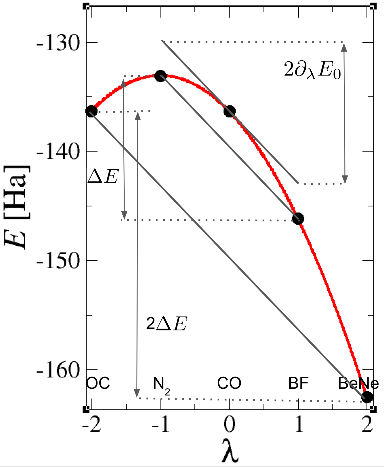
Figure 1: Electronic energy as a continuous function of linear coupling parameter $\lambda$ for some iso-electronic charge neutral diatomics with 14 protons. N₂ and BF correspond to alchemical diastereomers of CO, implying that the leading order term of their energy difference $\Delta E$ corresponds to twice the corresponding Hellmann-Feynman derivative evaluated for CO (See Eq. 1). The relative energy between more distant alchemical diastereomers CO and BeNe is twice that amount.

Note how this expansion recovers the case of alchemical chirality von Rudorff and von Lilienfeld (2021) (where first order terms vanish) whenever the perturbing Hamiltonian and the reference system are chosen such that the parity of $\rho_{0}$ and anti-parity of $\Delta v$ result in an overlap integral that exactly averages out. Due to the reflection plane in the reference Hamiltonian’s external potential and due to the energetic degeneracy up to third order, the iso-electronic compounds corresponding to $\hat{H}_{l}$ and $\hat{H}_{r}$ were dubbed ‘alchemical enantiomers’. However, the alchemical chirality symmetry condition with vanishing Hellmann-Feynman derivatives is not met when transmutating atoms with differing chemical environments. And thus, in the more general case the non-vanishing values for the Hellmann-Feynman derivative at the reference system become the leading order contributions to energy differences of arbitrary iso-electronic compound pairs. Correspondingly, we dub the latter ‘alchemical diastereomers’. In other words, alchemical diastereomers become enantiomers with approximate energy degeneracy whenever the relevant transmutating atoms in their averaged Hamiltonian posses the same chemical environment.

It is also noteworthy that the antisymmetry of the perturbation leads to the alternating signs in the left hand side expansion which, in turn, results in the cancellation of the even order terms in Eq. 1. Such alternations are frequently exploited, cf. the time reversal symmetry within molecular dynamics simulation when using the Verlet algorithm: Velocity and higher odd order time derivatives cancel and based on previous and current position, force based classical Newtonian propagation is exact up to 4th order Frenkel and Smit (2002). Accordingly if $E_{l}$ was also known, one could estimate $E_{r}$ as follows

$$E_{r} = 2E_{0}-E_{l}+\partial^{2}_{\lambda}E_{0}+\frac{1}{12}\partial^{4}_{\lambda}E_{0}+...$$ (2)

where all odd order terms have vanished — in complete analogy to Verlet’s integration. Correspondingly, this approach might be beneficial when the electron density perturbation is available, (for example from coupled perturbed self-consistent field calculation Lesiuk et al. (2012)), and yield $E_{r}$ exactly up to fourth order.

Perturbing the electronic density for the averaged Hamiltonian (in complete analogy to the energy above), we can see the connection to Levy’s estimation of iso-electronic energy differences

$$\Delta E \approx \int d{\bf r}\,\Delta v({\bf r})\,\bar{\rho}({\bf r})$$ (3)

that relies on the averaged electron densities, $\bar{\rho}=(\rho_{r}+\rho_{l})/2$. Levy (1978b) Consider

$$\rho_{+} = \rho_{0}+\partial_{\lambda}\rho_{0}+\frac{1}{2}\partial^{2}_{\lambda}\rho_{0}+\frac{1}{6}\partial^{3}_{\lambda}\rho_{0}+\frac{1}{24}\partial^{4}_{\lambda}\rho_{0}...$$

$$\rho_{-} = \rho_{0}-\partial_{\lambda}\rho_{0}+\frac{1}{2}\partial^{2}_{\lambda}\rho_{0}-\frac{1}{6}\partial^{3}_{\lambda}\rho_{0}+\frac{1}{24}\partial^{4}_{\lambda}\rho_{0}...$$ (4)

Averaging, and insertion in Levy’s formula, yields

$$\int d{\bf r}\,\Delta v({\bf r})\,\bar{\rho}({\bf r}) = \int d{\bf r}\Delta v({\bf r})\left(\rho_{0}+\frac{1}{2}\partial^{2}_{\lambda}\rho_{0}+\frac{1}{24}\partial^{4}_{\lambda}\rho_{0}+...\right)$$

for which the even order terms have also vanished. Term-wise comparison to Eq. 1 indicates that while Levy’s formula recovers the first order energy term, i.e. Eq. 6, exactly, it overestimates the third, fifth, and seventh order energy terms respectively by factors 3, 5, and 7, etc.etc. This implies that Levy’s approximation should be less accurate than the first order term in Eq. 1.

III Results and discussions

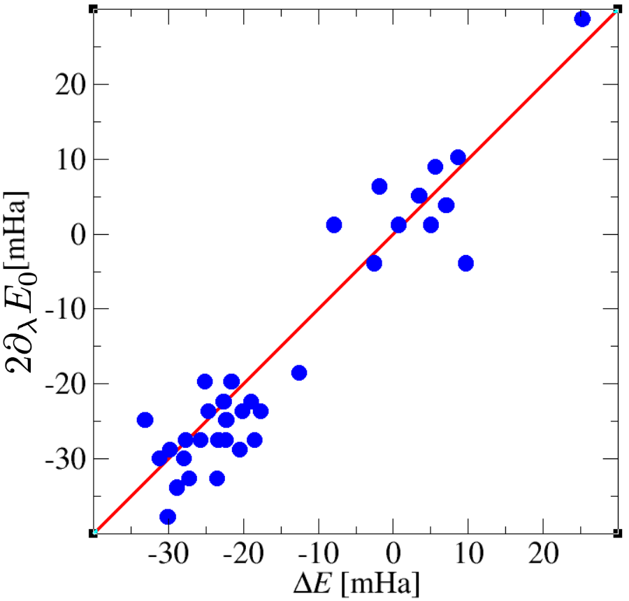
Figure 2: Estimated total energy difference ($2\partial_{\lambda}E$) vs. SCF based total energy difference ($\Delta E$) for 35 anti-symmetric BN doped alchemical diastereomers of toluene (mean absolute error = 4.3 mHa).

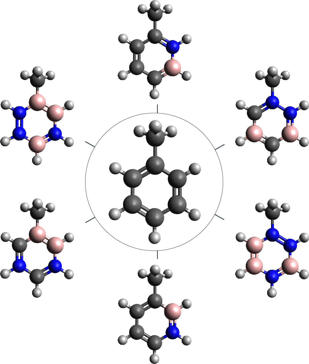
Figure 3: Three randomly selected dimensions in chemical space defining three pairs of alchemical diasteomers of toluene (out of the 35 dimensions for which relative energies are shown in Fig. 2). Alchemical diastereomers are placed opposite from each other in order to underscore their mutual relation in terms of antisymmetric alchemical perturbations of toluene as the joint averaged reference Hamiltonian, and with the lines indicating the corresponding dimension in chemical compound space.

Truncating the expansion Eq. 1 after the leading order term, we have numerically evaluated the predictive power when estimating the energy difference as

$$\Delta E \approx 2\partial_{\lambda}E_{0}\;=\;\int d{\bf r}\Delta v({\bf r})\rho_{0}({\bf r})$$ (6)

Fig. 1 provides a graphical illustration of this idea: Due to the antisymmetry condition of the perturbation, the slope at the reference system provides a first order estimate of the energy difference between the diastereomers. We note that if the energy was parabolic in $\lambda$, this estimate would become exact.

In Tab 1, numerical predictions of Eq. 6 and of Levy’s formula are shown for diatomics. Fair agreement, albeit not chemically accurate, is found despite some of the perturbations being very substantial. As expected from above analysis, Eq. 6 provides a systematically better estimate of the actual energy difference than Levy’s formula. This is encouraging since it requires the SCF procedure to obtain the electron density only for one (averaged reference) system, rather than for each of the two end-points as it is necessary for Levy.

If sufficiently accurate, the usefulness of this approximation could be considerable: It would imply that given the electron density of a reference systems, energy differences resulting from any of its combinatorially many possible antisymmetric alchemical perturbations could be estimated with negligible overhead merely by evaluating the corresponding Hellmann-Feynman derivatives. In other words, relative energy estimates for an arbitrarily large set of alchemical diastereomers, defined by their respective $\{\lambda_{i}\}$-perturbations, can be generated for negligible additional computational cost—as long as they all share the same averaged reference Hamiltonian. We have numerically exemplified this point for the BN doping of the aromatic moiety in the molecule toluene. In this case, BN doping defines 35 $\lambda$-dimensions space, along which we have estimated all the respective energy differences between the corresponding alchemical diastereomers — for ‘free’, i.e. via Eq. 6 and only based on the electron density obtained for the joint averaged reference Hamiltonian of toluene. Figs. 2 shows a scatter plot of the numerical estimates of energy differences between 35 pairs of alchemical diastereomers of toluene. The resulting MAE is 4.3 mHa which is close to chemical accuracy ($\sim$1 kcal/mol) and similar to the accuracy of hybrid density functional approximations. Fig. 3 exemplifies the central role of the averaged reference Hamiltonian of toluene for three pairs of alchemical diastereomers.

$\hat{H}_{l}$-$\hat{H}_{0}$-$\hat{H}_{r}$	$\Delta E$[Ha]	$2\partial_{\lambda}E_{0}$ [Ha]	Levy [Ha]Levy (1979)
NN-CO-BF	13.176560	13.196927	13.123976
NN-BF-LiNa	52.201112	52.495903	51.669013
NN-BeNe-HAl	115.963855	117.201259	112.968808
CO-BF-BeNe	26.207973	26.247951	26.132007
CO-BeNe-HeMg	77.811426	78.134173	77.094902
CO-LiNa-Si	152.885958	155.007039	148.255308
BF-BeNe-LiNa	39.024551	39.067086	38.958482
BF-LiNa-HAl	102.787295	103.338026	101.560490
BeNe-LiNa-HeMg	51.603454	51.669013	51.482530
BeNe-HeMg-Si	126.677985	127.795948	124.707031
LiNa-HeMg-HAl	63.762743	63.897974	63.490776
HeMg-HAl-Si	75.074531	75.312538	74.768959

Table 1: Relative electronic potential energy estimates between first and third diatomics. $2\partial_{\lambda}E_{0}$ corresponds to Eq. 6, whereas Levy corresponds to Eq. 3 Levy (1979). Numbers obtained at 1.1 Å interatomic distance using the PBE0 functional in the pcX-2 basis.

IV Computational Details

All numerical calculations were done using PySCF Sun et al. (2017); Harris et al. (2020); Pérez and Granger (2007) with the PBE0 density functional approximation Perdew et al. (1996); Ernzerhof and Scuseria (1999); Adamo and Barone (1999). The importance of basis set effects on alchemical interpolations having been established previously Domenichini et al. (2020); Domenichini and von Lilienfeld (2022), we have used Jensen’s pc2 basis set for hydrogens Jensen (2001, 2002), and the universal pcX-2 basis by Ambroise and Jensen for all other atoms Ambroise and Jensen (2019). The interatomic distance of all systems in the diatomics series was set to 1.1Å. The geometry of the 70 BN doped toluene derivatives was kept fixed to the equilibrium geometry of toluene obtained at the same level of theory and using Hermann’s geometry optimizer PyBerny Hermann (2020); it is shown in Tab. 2.

Atom	X [Å]	Y [Å]	Z [Å]
H	-0.00048	2.76025	1.05495
H	0.88360	2.79792	-0.46619
H	-0.88315	2.79793	-0.46700
C	-0.00000	2.38982	0.02594
C	0.00001	0.89122	-0.00419
C	1.19407	0.17608	-0.00721
C	-1.19407	0.17608	-0.00705
C	1.19708	-1.21024	-0.00623
C	-0.00000	-1.90984	-0.00527
C	-1.19708	-1.21023	-0.00606
H	2.13561	0.71445	-0.01262
H	2.13883	-1.74590	-0.01129
H	-0.00000	-2.99283	-0.00868
H	-2.13883	-1.74589	-0.01100
H	-2.13560	0.71446	-0.01235

Table 2: Optimized atomic coordinates of toluene.

V Conclusion

We have generalized the alchemical chirality concept towards the notion of alchemical antisymmetric perturbations that result in vanishing even order contributions to the relative energies of alchemical diastereomers. Our analysis also provides an interpretation of Levy’s formula Levy (1979). Numerical evidence suggests that the leading first order term gives meaningful, and sometimes even accurate, estimates of energy differences between alchemical diastereomers that are close to each other. The choice of the averaged reference system is key, it defines the number of dimensions in chemical space along which energy differences between alchemical diastereomers can be estimated with negligible computational overhead. We have exemplified this point for 35 BN doped alchemical diastereomers of toluene for which energy differences were calculated using 35 Hellmann-Feynman derivates with the same single electron density and yielding a mean absolute error of only 4.3 mHa. Future studies will deal with the role of the quality of the electron density used within the Hellmann-Feynman derivative, with the correlation between prediction error and magnitude of perturbation, and the importance of higher order terms.