Efficient and Multiply Robust Risk Estimation
under General Forms of Dataset Shift

Abstract

Statistical machine learning methods often face the challenge of limited data available from the population of interest. One remedy is to leverage data from auxiliary source populations, which share some conditional distributions or are linked in other ways with the target domain. Techniques leveraging such dataset shift conditions are known as domain adaptation or transfer learning. Despite extensive literature on dataset shift, limited works address how to efficiently use the auxiliary populations to improve the accuracy of risk evaluation for a given machine learning task in the target population.

In this paper, we study the general problem of efficiently estimating target population risk under various dataset shift conditions, leveraging semiparametric efficiency theory. We consider a general class of dataset shift conditions, which includes three popular conditions—covariate, label and concept shift—as special cases. We allow for partially non-overlapping support between the source and target populations. We develop efficient and multiply robust estimators along with a straightforward specification test of these dataset shift conditions. We also derive efficiency bounds for two other dataset shift conditions, posterior drift and location-scale shift. Simulation studies support the efficiency gains due to leveraging plausible dataset shift conditions.

1 Introduction

1.1 Background

A common challenge in statistical machine learning approaches to prediction is that limited data is available from the population of interest, despite potentially large amounts of data from similar populations. For instance, it may be of interest to predict HIV treatment response in a community based on only a few observations. A large dataset from another community in a previous HIV study may help improve the training of such a prediction model. Another example is building a classification or diagnosis model based on medical images for lung diseases (Christodoulidis et al., 2017). A key task therein is to classify the texture in the image, but the size of a labeled medical image sample is often limited due to the high cost of data acquisition and labeling. It may be helpful to leverage large existing public image datasets as supplemental data to train the classifier.

In these examples and others, it is desirable to use data from similar source populations to supplement target population data, under plausible dataset shift conditions relating the source and target populations (see, e.g., Storkey, 2013; Shimodaira, 2000; Sugiyama and Kawanabe, 2012). Such methods are known as domain adaptation or transfer learning (see, e.g. Kouw and Loog, 2018; Pan and Yang, 2010).

A great deal of work has been devoted to leveraging or addressing various dataset shift conditions. Polo et al. (2022) proposed testing for various forms of dataset shift. Among dataset shift types, popular conditions include covariate shift, where only the covariate distribution changes, as well as label shift, where only the outcome distribution changes—also termed choice-based sampling or endogenous stratified sampling in Manski and Lerman (1977), prior probability shift in Storkey (2013), and target shift in Scott (2019); Zhang et al. (2013). Another popular condition is concept shift, where the covariate or label distribution does not change—also termed conditional shift in Zhang et al. (2013). See, e.g., Kouw and Loog (2018); Moreno-Torres et al. (2012); Schölkopf et al. (2012), for reviews of common dataset shift conditions. These three conditions—covariate, label, and concept shift—are popular because they are interpretable, broadly applicable, and analytically tractable.

Other conditions and methods have also been studied for more specific problems; examples include (generalized, penalized) linear models (Bastani, 2021; Cai et al., 2022; Chakrabortty and Cai, 2018; Gu et al., 2022; Liu et al., 2020b, 2023b; Tian and Feng, 2022; Zhang et al., 2019, 2022; Zhou et al., 2022), binary classification (Cai and Wei, 2021; Scott, 2019), graphical models (He et al., 2022; Li et al., 2022), and location-scale shifts (Zhang et al., 2013), among others.

For domain adaptation where a limited amount of fully observed data from the target population is available, there may be multiple valid methods to incorporate source population data. It is thus important to understand which ones efficiently extract information from data in both source and target populations. However, the efficient use of source population data to supplement the target population data has only been recently studied. Azriel et al. (2021); Gronsbell et al. (2022); Yuval and Rosset (2023); Zhang et al. (2021); Zhang and Bradic (2022) studied this problem for mean estimation and (generalized) linear models, under concept shift (i.e., for semi-supervised learning). Li and Luedtke (2023) studied efficiency theory for data fusion with an emphasis on causal inference applications, a setting related to ours with a somewhat different primary objective. Other related works in data fusion include Angrist and Krueger (1992); Chatterjee et al. (2016); Chen and Chen (2000); D’Orazio et al. (2006, 2010); Evans et al. (2021); Rässler (2012); Robins et al. (1995), among others. A study of domain adaptation with more general prediction techniques under general dataset shift conditions is lacking.

1.2 Our contributions

In this paper, we study the general problem of efficient model-agnostic risk estimation in a target population for data adaptation with fully observed data from both source and target populations under various dataset shift conditions. We take the perspective of modern semiparametric efficiency theory (see, e.g., Bolthausen et al., 2002; Pfanzagl, 1985, 1990; van der Vaart, 1998), because many dataset shift conditions can be formulated as restrictions on the observed data generating mechanism, yielding a semiparametric model.

We estimate the risk due to its broad applicability and central role in training predictive models. For example, given several candidate predictors, it might be desirable to compare their prediction performance via an estimate of risk such as mean squared error. Reducing variability in this risk estimator by efficiently leveraging source populations improves our ability to discriminate between candidate models to select the optimal learner for the target population. Thus, training a prediction model by minimizing an efficient estimator of the risk might lead to more precise predictions (see, e.g., Theorem 3.2.5 of van der Vaart and Wellner, 1996). Likewise, the related goal of constructing prediction sets with guaranteed coverage (Vovk, 2013; Qiu et al., 2022; Yang et al., 2022) often depends on precise estimates of the coverage error probability of constructed prediction sets (Angelopoulos et al., 2021; Park et al., 2020, 2022; Yang et al., 2022).

After presenting the general problem setup in Section 2, we consider a general dataset shift condition, which we call sequential conditionals (Condition DS.0 in Section 3), for scenarios where target population data is available while the source and target populations may have only partially overlapping support. This condition includes covariate, label and concept shift as special cases. We consider data where an observation $Z$ can be decomposed into components $(Z_{1},\ldots,Z_{K})$. Under this condition, some of the conditional distributions $Z_{k}\mid(Z_{1},\ldots,Z_{k-1})$ are shared between the target and source populations, for $k=1,\ldots,K$. As our first main contribution, we propose a novel risk estimator that we formally show in Theorem 1 to be semiparametrically efficient and multiply robust (Tchetgen Tchetgen, 2009; Vansteelandt et al., 2007) under this dataset shift condition.

In particular, we propose to obtain flexible estimators $\hat{\theta}^{k}$ of certain nuisance conditional odds functions $\theta^{k}_{*}$ conditional on variables $(Z_{1},\ldots,Z_{k})$, and estimators $\hat{\ell}^{k}$ of conditional mean loss functions $\ell^{k}_{*}$ by sequential regression of $\hat{\ell}^{k+1}(Z_{1},\ldots,Z_{k+1})$ on $(Z_{1},\ldots,Z_{k})$. We show that our risk estimator is efficient given sufficient convergence rates of the product of errors of (i) $\hat{\theta}^{k}$ for $\theta^{k}_{*}$, and of (ii) $\hat{\ell}^{k}$ for $\ell^{k}_{*}$. Moreover, when $\hat{\ell}^{k}_{v}$ converges to a certain limit function $\ell^{k}_{\infty}$, our estimator is $2^{K-1}$-robust. Specifically, it is consistent if for every $k=1,\ldots,K-1$, $\hat{\theta}^{k}$ is consistent for $\theta^{k}_{*}$ or $\hat{\ell}^{k}$ is consistent for the oracle regression $u^{k}$ of $\ell^{k}_{\infty}$; but not necessarily both. The latter oracle regression is defined as the conditional expectation of $\ell^{k}_{\infty}$ on $(Z_{1},\ldots,Z_{k})$ under the true distribution.

Our choice of parametrization and the sequential construction of $\hat{\ell}^{k}$ are key to multiple robustness. Suppose instead that each true conditional mean loss function $\ell^{k}_{*}$ is instead parameterized directly—rather than sequentially—as the regression of the loss on the variables $(Z_{1},\ldots,Z_{k})$ in the target population, and accordingly construct $\hat{\ell}^{k}$ by direct regression in the target population. Then the resulting estimating equation-based estimator using the efficient influence function is not guaranteed to be $2^{K-1}$-robust.

Based on this estimator, we further propose a straightforward specification test (Hausman, 1978) of whether our efficient estimator converges to the risk of interest in probability, which can be used to test the assumed sequential conditionals condition. In doing so, we theoretically analyze the behavior of our proposed estimator when the sequential conditionals condition fails. We analytically derive the bias due to the failure of sequential conditionals and show that, in this case, our estimator may diverge arbitrarily as sample size increases if the support of the source populations only partially overlaps with the target population. Under the sequential conditionals condition, such a scenario for the supports is allowed, but does not lead to this convergence issue. To obtain this result, we need a more careful analysis than the standard analysis of Z-estimators (e.g., Section 3.3 in van der Vaart and Wellner, 1996) because of the inconsistency of our estimator without the sequential conditionals consirion.

Next, we investigate the efficient risk estimation problem in more detail for concept shift in the features and for covariate shift, in Sections 4 and 5, respectively. We characterize when efficiency gains are large, develop simplified efficient and robust estimators, and study their empirical performance in simulation studies. In particular, we show that our estimator is regular and asymptotically linear (RAL) even if the nuisance function is estimated inconsistently under concept shift (Theorem 2). We also show a new impossibility result about such full robustness for covariate or label shift under common parametrizations (Lemma 1). In Section 6, we derive efficiency bounds for risk estimation under two other widely-applicable dataset shift conditions, posterior drift (Scott, 2019) and location-scale shift (Zhang et al., 2013). The proof of these results requires delicate derivations involving tangent spaces and their orthogonal complements, leading to intricate linear integral equations and, in some cases, a closed-form solution for the efficient influence functions.

We present additional new results in the Supplementary Material. In Supplement S2, we present a generalized version of the dataset shift condition from Section 3 that allows the target population data to be unavailable. We propose a similar estimator to that in Section 3 and show that it is efficient and multiply robust. In Supplement S3, studying concept shift in the labels and label shift, we present results analogous to those in Sections 4 and 5. In Supplement S6, we present additional results on other widely-applicable dataset shift conditions, including the invariant density ratio condition (Tasche, 2017) and stronger versions of posterior drift (Scott, 2019) and location-scale shift (Zhang et al., 2013) conditions. We illustrate our proposed estimators in an HIV risk prediction example in Supplement S7. In Supplement S8, we describe how our proposed risk estimators can help construct prediction sets with marginal or training-set conditional validity. Proofs of all theoretical results can be found in Supplement S9. We implement our proposed methods for covariate, label and concept shift in an R package available at https://github.com/QIU-Hongxiang-David/RiskEstDShift.

2 Problem setup

Let $O$ be a prototypical data point consisting of the observed data $Z$ lying in a space $\mathcal{Z}$ and an integer indexing variable $A$ in a finite set $\mathcal{A}$ containing zero. The variable $A$ indicates whether the data point comes from the target population ($A=0$) or a source population ($A\in\mathcal{A}\setminus\{0\}$). The observed data $(O_{1},\ldots,O_{n})$ is an independent and identically distributed (i.i.d.) sample from an unknown distribution $P_{*}$. We will use a subscript $*$ to denote components of $P_{*}$ throughout this paper. Data $Z$ is observed from both the source and target populations, i.e., for both $A=0$ and $A\neq 0$.

The estimand of interest is the risk, namely the average value of a given loss function $\ell:\mathcal{Z}\to\mathbb{R}$, in the target population:

$$r_{*}:=R(P_{*}):=\mathbb{E}_{P_{*}}[\ell(Z)\mid A=0].$$ (1)

We often focus on the supervised setting where $Z=(X,Y)$, with $X\in\mathcal{X}$ being the covariate or feature and $Y\in\mathcal{Y}$ being the outcome or label. In this case, our observed data are i.i.d. triples $(X_{i},Y_{i},A_{i})\in\mathcal{X}\times\mathcal{Y}\times\mathcal{A}$ distributed according to $P_{*}$. Next, we provide two examples of loss functions $\ell$ below.

Example 1 (Supervised learning/regression).

Let $f:\mathcal{X}\to\mathcal{Y}^{\prime}$ be a given predictor—obtained, for example, from a separate training dataset—for some space $\mathcal{Y}^{\prime}$ that can differ from $\mathcal{Y}$. It may be of interest to estimate a measure of the accuracy of $f$. One common measure is the mean squared error, which is induced by the squared error loss $\ell(x,y)=(y-f(x))^{2}$. For binary outcomes where $\mathcal{Y}=\{0,1\}$, it is also common to consider the risk induced by the cross-entropy loss, namely Bernoulli negative log-likelihood $\ell(x,y)=-y\log\{f(x)\}-(1-y)\log\{1-f(x)\}$, when $\mathcal{Y}^{\prime}$ is the unit interval $(0,1)$ and $f$ outputs a predicted probability. Another common measure of risk is $P_{*}(Y\neq f(X)\mid A=0)$, measuring prediction inaccuracy. This is induced by the loss $\ell(x,y)={\mathbbm{1}}(y\neq f(x))$ when $\mathcal{Y}^{\prime}=\{0,1\}$ and $f$ outputs a predicted label.

Example 2 (Prediction sets with coverage guarantees).

It is often of interest to construct prediction sets with a coverage guarantee. Two popular guarantees are marginal coverage and training-set conditional—or probably approximately correct (PAC)—coverage (Vovk, 2013; Park et al., 2020). To achieve such coverage guarantees, one may estimate—or obtain a confidence interval for—the coverage error of a given prediction set (Vovk, 2013; Angelopoulos et al., 2021; Yang et al., 2022). Let $C:\mathcal{X}\to 2^{\mathcal{Y}}$ be a given prediction set. With the indicator loss $\ell(x,y)={\mathbbm{1}}(y\notin C(x))$, the associated risk is the coverage error probability $P_{*}(Y\notin C(X)\mid A=0)$ of $C$ in the target population.

Remark 1 (Broader interpretation of risk estimation problem).

Our results in this paper apply to a broader range of problems beyond risk estimation, provided that the problem under consideration can be mapped to our setup. For example, the loss function $\ell$ may be interpreted in a broad sense. If the estimand of interest is the mean $\mathbb{E}_{P_{*}}[Z\mid A=0]$ for $Z\in\real$, we may take $\ell$ to be the identity function; to estimate a quantile of $Z\mid A=0$, we may consider $\ell$ ranging over the function class $\{z\mapsto{\mathbbm{1}}(z\leq t):t\in\real\}$. As another example, the data point $Z$ does not necessarily have to consist of a covariate vector $X$ and an outcome $Y$. If additional variables $W$ related to $Y$ are observed—for example, outcomes other than $Y$—these can be leveraged for risk estimation, even if the prediction model only uses the covariate $X$, see Example 3 in Section 3.

Without additional conditions on the true data distribution $P_{*}$—under a nonparametric model—the source populations are non-informative about the target population because they may differ arbitrarily. In this case, a viable estimator of $r_{*}$ is the nonparametric estimator, the sample mean over the target population data:

$$\hat{r}_{{\mathrm{np}}}:=\frac{\sum_{i=1}^{n}{\mathbbm{1}}(A_{i}=0)\ell(Z_{i})}{\sum_{i=1}^{n}{\mathbbm{1}}(A_{i}=0)}.$$ (2)

For any scalars $\rho\in(0,1)$ and $r\in\real$, we define

$$D_{\mathrm{np}}(\rho,r):o=(z,a)\mapsto\frac{{\mathbbm{1}}(a=0)}{\rho}\{\ell(z)-r\}.$$ (3)

We denote $\rho_{*}:=P_{*}(A=0)\in(0,1)$, the true proportion of data from the target population. It is not hard to show that $D_{\mathrm{np}}$ is the influence function of $\hat{r}_{{\mathrm{np}}}$; $\hat{r}_{{\mathrm{np}}}$ is asymptotically semiparametrically efficient under a nonparametric model and $\sqrt{n}(\hat{r}_{{\mathrm{np}}}-r_{*})\overset{d}{\to}\mathrm{N}(0,\sigma_{*,{\mathrm{np}}}^{2})$ with $\sigma_{*,{\mathrm{np}}}^{2}:=\mathbb{E}_{P_{*}}[D_{\mathrm{np}}(\rho_{*},r_{*})$$(O)^{2}]$; see Supplement S9.2.

The nonparametric estimator $\hat{r}_{{\mathrm{np}}}$ ignores data from the source population. If limited data from the target population is available, namely $P_{*}(A=0)$ is small, this estimator might not be accurate. This motivates using source population data and plausible conditions to obtain more accurate estimators.

Notations and terminology. We next introduce some notation and terminology. We will use the terms “covariate” and “feature” interchangeably, and similarly for “label” and “outcome”. For any non-negative integers $M$ and $N$, we use $[M:N]$ to denote the index set $\{M,M+1,\ldots,N\}$ if $M\leq N$ and the empty index set otherwise; we use $[M]$ as a shorthand for $[1:M]$. For any finite set $S$, we use $|S|$ to denote its cardinality.

For a distribution $P$, we use $P_{\sharp}$ and $P_{\sharp\mid\natural}$ to denote the marginal distribution of the random variable $\sharp$ and the conditional distribution of $\sharp\mid\natural$, respectively, under $P$; we use $P_{*,\sharp}$ and $P_{*,\sharp\mid\natural}$ to denote these distributions under $P_{*}$. We use $P^{n}$ to denote the empirical distribution of a sample of size $n$ from $P$. When splitting the sample into $V>0$ folds, we use $P^{n,v}$ and $P_{\sharp}^{n,v}$ to denote empirical distributions in fold $v\in[V]$. All functions considered will be measurable with respect to appropriate sigma-algebras, which will be kept implicit. For any function $f$, any distribution $P$, and any $p\in[1,\infty]$, we use $\|f\|_{L^{p}(P)}$ to denote the $L^{p}(P)$ norm of $f$, namely $(\int f(x)^{p}P({\mathrm{d}}x))^{1/p}$. We also use $L^{p}(P)$ to denote the space of all functions with a finite $L^{p}(P)$ norm, and use $L^{p}_{0}(P)$ to denote $\{f\in L^{p}(P):\int f{\mathrm{d}}P=0\}$. All asymptotic results are with respect to the sample size $n$ tending to infinity.

We finally review a few concepts and basic results that are central to semiparametric efficiency theory. More thorough introductions can be found in Bickel et al. (1993); Bolthausen et al. (2002); Pfanzagl (1985, 1990); van der Vaart (1998). An estimator $\hat{\theta}$ of a parameter $\theta_{*}=\theta_{*}(P_{*})$ is said to be asymptotically linear if $\hat{\theta}=\theta_{*}+n^{-1}\sum_{i=1}^{n}{\mathrm{IF}}(O_{i})+{\mathrm{o}}_{p}(n^{-1/2})$ for a function ${\mathrm{IF}}\in L^{2}_{0}(P_{*})$. This asymptotic linearity implies that $\sqrt{n}(\hat{\theta}-\theta_{*})\overset{d}{\to}\mathrm{N}(0,\mathbb{E}_{P_{*}}[{\mathrm{IF}}(O)^{2}])$. The function ${\mathrm{IF}}$ is called the influence function of $\hat{\theta}$. Under a semiparametric model, there may be infinitely many influence functions, but there exists a unique efficient influence function, which is the influence function of regular asymptotically linear (RAL) estimators with the smallest asymptotic variance. Under a nonparametric model, all RAL estimators of a parameter $\theta_{*}$ share the same influence function, which equals the efficient influence function.

3 Cross-fit estimation under a general dataset shift condition

3.1 Statement of condition and efficiency bound

We consider the following general dataset shift condition characterized by sequentially identical conditional distributions. Under this condition, some auxiliary source population datasets are informative about one component of the target population. We allow $Z$ to be a general random variable rather than just $(X,Y)$ and allow more than one source population to be present. Thus, let $Z$ be decomposed into $K\geq 1$ components $(Z_{1},\ldots,Z_{K})$. Define $\bar{Z}_{0}:=\emptyset$, $\bar{Z}_{k}:=(Z_{1},\ldots,Z_{k})$, and $\mathcal{Z}_{k-1}$ to be the support of $\bar{Z}_{k-1}\mid A=0$ for $k\in[K]$. The condition is as follows.

Condition DS.0 (Sequential conditionals).

For every $k\in[K]$, there exists a known subset $\mathcal{S}_{k}\subset\mathcal{A}\setminus\{0\}$ such that, for all $a\in\mathcal{S}_{k}$, $Z_{k}\mid\bar{Z}_{k-1}=\bar{z}_{k-1},A=a$ is distributed identically to $Z_{k}\mid\bar{Z}_{k-1}=\bar{z}_{k-1},A=0$ for all $\bar{z}_{k-1}$ in the intersection of $\mathcal{Z}_{k-1}$ and the support of $\bar{Z}_{k-1}\mid A=a$.

We use $\mathcal{S}^{\prime}_{k}$ to denote $\{0\}\cup\mathcal{S}_{k}$ for short. This condition states that conditionally on $A\in\mathcal{S}^{\prime}_{k}$, $Z_{k}$ is independent of $A$ given $\bar{Z}_{k-1}$. Equivalently, it states that every conditional distribution $Z_{k}\mid\bar{Z}_{k-1},A=0$ ($k\in[K]$) is equal to that in the source populations with $a\in\mathcal{S}_{k}$. We show an example of this condition in Figure 1. In particular, we allow for cases where no source population exists to supplement learning some conditional distributions, that is, $\mathcal{S}_{k}$ may be empty for some $k$. We also allow irrelevant variables in some source populations to be missing; for example, in Figure 1, $(Z_{3},Z_{4},Z_{5})$ in the source population $A=2$ may be missing as these variables are not assumed to be informative about the target population.

According to the well-known review by Moreno-Torres et al. (2012), the following four dataset shift conditions are among the most widely considered when one source population is available, so that $\mathcal{A}=\{0,1\}$. These conditions are all special cases of Condition DS.0.

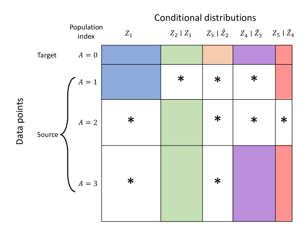
Figure 1: Illustration of Condition DS.0 with $K=5$. In each column, cells sharing the same color represent the same conditional distribution, while cells with asterisks represent conditional distributions that may arbitrarily differ from the target population ($A=0$). In this example, $\mathcal{S}_{1}=\{1\}$, $\mathcal{S}_{2}=\{2,3\}$, $\mathcal{S}_{3}=\emptyset$, $\mathcal{S}_{4}=\{3\}$, and $\mathcal{S}_{5}=\{1,3\}$.

Condition DS.1 (Concept shift in the features).

$X\mathchoice{\mathrel{\hbox to0.0pt{$\displaystyle\perp$\hss}\mkern 2.0mu{\displaystyle\perp}}}{\mathrel{\hbox to0.0pt{$\textstyle\perp$\hss}\mkern 2.0mu{\textstyle\perp}}}{\mathrel{\hbox to0.0pt{$\scriptstyle\perp$\hss}\mkern 2.0mu{\scriptstyle\perp}}}{\mathrel{\hbox to0.0pt{$\scriptscriptstyle\perp$\hss}\mkern 2.0mu{\scriptscriptstyle\perp}}}A$.

Condition DS.2 (Concept shift in the labels).

$Y\mathchoice{\mathrel{\hbox to0.0pt{$\displaystyle\perp$\hss}\mkern 2.0mu{\displaystyle\perp}}}{\mathrel{\hbox to0.0pt{$\textstyle\perp$\hss}\mkern 2.0mu{\textstyle\perp}}}{\mathrel{\hbox to0.0pt{$\scriptstyle\perp$\hss}\mkern 2.0mu{\scriptstyle\perp}}}{\mathrel{\hbox to0.0pt{$\scriptscriptstyle\perp$\hss}\mkern 2.0mu{\scriptscriptstyle\perp}}}A$.

Condition DS.3 (Full-data covariate shift).

$Y\mathchoice{\mathrel{\hbox to0.0pt{$\displaystyle\perp$\hss}\mkern 2.0mu{\displaystyle\perp}}}{\mathrel{\hbox to0.0pt{$\textstyle\perp$\hss}\mkern 2.0mu{\textstyle\perp}}}{\mathrel{\hbox to0.0pt{$\scriptstyle\perp$\hss}\mkern 2.0mu{\scriptstyle\perp}}}{\mathrel{\hbox to0.0pt{$\scriptscriptstyle\perp$\hss}\mkern 2.0mu{\scriptscriptstyle\perp}}}A\mid X$.

Condition DS.4 (Full-data label shift).

$X\mathchoice{\mathrel{\hbox to0.0pt{$\displaystyle\perp$\hss}\mkern 2.0mu{\displaystyle\perp}}}{\mathrel{\hbox to0.0pt{$\textstyle\perp$\hss}\mkern 2.0mu{\textstyle\perp}}}{\mathrel{\hbox to0.0pt{$\scriptstyle\perp$\hss}\mkern 2.0mu{\scriptstyle\perp}}}{\mathrel{\hbox to0.0pt{$\scriptscriptstyle\perp$\hss}\mkern 2.0mu{\scriptscriptstyle\perp}}}A\mid Y$.

Condition DS.0 reduces to DS.1—concept shift in the features—by setting $K=2$, $\mathcal{A}=\{0,1\}$, $\mathcal{S}_{1}=\{1\}$, $\mathcal{S}_{2}=\emptyset$, $Z_{1}=X$, and $Z_{2}=Y$. Indeed, Condition DS.0 for $k=1$ states that $(Z_{1}|A=1)=_{d}(Z_{1}|A=0)$, or equivalently that $(X|A=1)=_{d}(X|A=0)$, which means that $X\mathchoice{\mathrel{\hbox to0.0pt{$\displaystyle\perp$\hss}\mkern 2.0mu{\displaystyle\perp}}}{\mathrel{\hbox to0.0pt{$\textstyle\perp$\hss}\mkern 2.0mu{\textstyle\perp}}}{\mathrel{\hbox to0.0pt{$\scriptstyle\perp$\hss}\mkern 2.0mu{\scriptstyle\perp}}}{\mathrel{\hbox to0.0pt{$\scriptscriptstyle\perp$\hss}\mkern 2.0mu{\scriptscriptstyle\perp}}}A$. Since $\mathcal{S}_{2}=\emptyset$, Condition DS.0 for $k=2$ does not impose additional constraints. Similarly, Condition DS.0 reduces to DS.2—concept shift in the labels—with the above choices but switching $Z_{1}=Y$ and $Z_{2}=X$.

Condition DS.0 reduces to DS.3—full-data covariate shift—by setting $K=2$, $\mathcal{A}=\{0,1\}$, $\mathcal{S}_{1}=\emptyset$, $\mathcal{S}_{2}=\{1\}$, $Z_{1}=X$, and $Z_{2}=Y$. Indeed, since $\mathcal{S}_{1}=\emptyset$, Condition DS.0 for $k=1$ does not impose constraints. For $k=2$, Condition DS.0 states that $(Z_{2}|Z_{1},A=1)=_{d}(Z_{2}|Z_{1},A=0)$, or equivalently that $(Y|X,A=1)=_{d}(Y|X,A=0)$, which means that $Y\mathchoice{\mathrel{\hbox to0.0pt{$\displaystyle\perp$\hss}\mkern 2.0mu{\displaystyle\perp}}}{\mathrel{\hbox to0.0pt{$\textstyle\perp$\hss}\mkern 2.0mu{\textstyle\perp}}}{\mathrel{\hbox to0.0pt{$\scriptstyle\perp$\hss}\mkern 2.0mu{\scriptstyle\perp}}}{\mathrel{\hbox to0.0pt{$\scriptscriptstyle\perp$\hss}\mkern 2.0mu{\scriptscriptstyle\perp}}}A\mid X$. Similarly, it reduces to DS.4—full-data label shift—with the above choices but switching $Z_{1}=Y$ and $Z_{2}=X$. We refer to Conditions DS.3 and DS.4 as full-data covariate and label shift, respectively, to emphasize that we have full observations $(X,Y,A)$ from the target population. For brevity, we refer to them as covariate or label shift when no confusion shall arise.

Condition DS.0 also includes more sophisticated dataset shift conditions and we provide a few examples below. See Supplement S1 for further examples.

Example 3 (Improving diagnosis with texture source data).

Christodoulidis et al. (2017) study diagnosing interstitial lung diseases (ILD) $Y$ based on computed tomography (CT) scans $X$ by training a classifier $f:x\mapsto f(x)\in\mathcal{Y}$. One key task in the diagnosis is to classify the texture $W$ revealed in the CT scan image $X$. Because of the high cost of collecting and human-labeling CT scans, Christodoulidis et al. (2017) leverage external texture source datasets ($A=1$) containing $(X,W)$ to train the predictive model. These source datasets were not built for diagnosing ILD and thus $Y$ is missing.

It may be reasonable to assume that the distribution of textures given the image is the same across the sample of CT scans and the source datasets, namely that $W|X=x,A=0$ and $W|X=x,A=1$ are identically distributed for $x$ in the common support of $X\mid A=0$ and $X\mid A=1$. This assumption corresponds to Condition DS.0 where $K=3$, $\mathcal{A}=\{0,1\}$, $Z_{1}=X$, $Z_{2}=W$, $Z_{3}=Y$, $\mathcal{S}_{2}=\{1\}$ and $\mathcal{S}_{1}=\mathcal{S}_{3}=\emptyset$.

Example 4 (Partial covariate shift).

Consider a full-data covariate shift setting with data $(X,Y)$ where the features $X=(X_{1},X_{2})$ consist of two components. Suppose that $X_{1}$ is known to be identically distributed in the two environments $A=0$ and $A=1$. For instance, an investigator might be interested in image classification where the environment only partially shifts. Such a partial shift may occur when the distribution of the weather—represented by extracted features $X_{2}$— changes, but the distribution of the objects—represented by other extracted features $X_{1}$—in the images is unchanged (e.g., Robey et al., 2020, etc.). This assumption corresponds to Condition DS.0 with $K=3$, $Z_{1}=X_{1}$, $Z_{2}=X_{2}$, $Z_{3}=Y$, $\mathcal{A}=\{0,1\}$, $\mathcal{S}_{1}=\{1\}$, $\mathcal{S}_{2}=\emptyset$, and $\mathcal{S}_{3}=\{1\}$.

In our problem, a plug-in estimation approach could be to pool all data sets that share the same conditional distributions for each $k$, namely $A\in\mathcal{S}^{\prime}_{k}$, and estimating these distributions nonparametrically. Then, the risk can be estimated by integrating the loss over the estimated distribution. However, as it is well known, this approach can suffer from a large bias or may limit the choice of distribution or density estimators, and typically requires a delicate case-by-case analysis to establish its accuracy (e.g., McGrath and Mukherjee, 2022, etc.).

We now describe and review results on efficiency, which characterize the smallest possible asymptotic variance of a sequence of regular estimators under the dataset shift condition DS.0. This will form the basis of our proposed estimator in the next section. We first introduce a few definitions. Define the conditional probability of each population

$$\Pi^{k,a}_{*}:\bar{z}_{k}\mapsto P_{*}(A=a\mid\bar{Z}_{k}=\bar{z}_{k})\ \ \text{for }k\in[0:K-1],\,a\in\mathcal{A},$$

and let $\pi^{a}_{*}:=\Pi^{0,a}_{*}=P_{*}(A=a)$ denote the marginal probabilities of all populations ($a\in\mathcal{A}$); thus, $\pi^{0}_{*}=\rho_{*}$ for $\rho_{*}$ from Section 2. Define the conditional odds of relevant source populations versus the target population:

$$\theta^{k-1}_{*}:=\frac{\sum_{a\in\mathcal{S}_{k}}\Pi^{k-1,a}_{*}}{\Pi^{k-1,0}_{*}}\ \ \text{for }k\in[K].$$

We also define conditional means of the loss starting with $\ell^{K}_{*}:=\ell$ and letting recursively

$$\ell^{k}_{*}:\bar{z}_{k}\mapsto\mathbb{E}_{P_{*}}[\ell^{k+1}_{*}(\bar{Z}_{k+1})\mid\bar{Z}_{k}=\bar{z}_{k},A\in\mathcal{S}^{\prime}_{k+1}]\ \ \text{for }\bar{z}_{k}\in\mathcal{Z}_{k},\ k\in[K-1].$$

We allow $\ell^{k}_{*}$ to take any value outside $\mathcal{Z}_{k}$, for example, when the support of $\bar{Z}_{k}\mid A\in\mathcal{S}^{\prime}_{k+1}$ is larger than the support $\mathcal{Z}_{k}$ of $\bar{Z}_{k}\mid A=0$. Under Condition DS.0, $\ell^{k}_{*}(\bar{z}_{k})=\mathbb{E}_{P_{*}}[\ell(Z)\mid\bar{Z}_{k}=\bar{z}_{k},A=0]$ for $\bar{z}_{k}\in\mathcal{Z}_{k}$. We discuss the consequences of the non-unique definition of $\ell^{k}_{*}$ without Condition DS.0 in more detail in Section 3.4. Let $\bm{\ell}_{*}:=(\ell^{k}_{*})_{k=1}^{K-1}$, $\bm{\theta}_{*}:=(\theta^{k}_{*})_{k=1}^{K-1}$, and $\bm{\pi}_{*}:=(\pi^{a}_{*})_{a\in\mathcal{A}}$ be collections of true nuisances. For any given collections $\bm{\ell}=(\ell^{k})_{k=1}^{K-1}$, $\bm{\theta}=(\theta^{k})_{k=1}^{K-1}$ and $\bm{\pi}:=(\pi^{a})_{a\in\mathcal{A}}$ of nuisances, a scalar $r$ and $\ell^{K}:=\ell$, define the pseudo-loss $\mathcal{T}(\bm{\ell},\bm{\theta},\bm{\pi}):\mathcal{O}\to\mathbb{R}$ based on these nuisances, so that for $o=(z,a)$,

$$\begin{split}\mathcal{T}(\bm{\ell},\bm{\theta},\bm{\pi})(o)=\sum_{k=2}^{K}\frac{{\mathbbm{1}}(a\in\mathcal{S}^{\prime}_{k})}{\pi^{0}(1+\theta^{k-1}(\bar{z}_{k-1}))}\left\{\ell^{k}(\bar{z}_{k})-\ell^{k-1}(\bar{z}_{k-1})\right\}+\frac{{\mathbbm{1}}(a\in\mathcal{S}^{\prime}_{1})}{\pi^{0}(1+\theta^{0})}\ell^{1}(z_{1}).\end{split}$$ (4)

The motivation for this transformation is similar to that for the unbiased transformation from Rotnitzky et al. (2006); Rubin and van der Laan (2007) and the pseudo-outcome from Kennedy (2020). Further, with $\theta^{0}:=\sum_{a\in\mathcal{S}_{1}}\pi^{a}/\pi^{0}$, define

$$D_{\mathrm{SC}}(\bm{\ell},\bm{\theta},\bm{\pi},r):o=(z,a)\mapsto\mathcal{T}(\bm{\ell},\bm{\theta},\bm{\pi})(o)-\frac{{\mathbbm{1}}(a\in\mathcal{S}^{\prime}_{1})}{\pi^{0}(1+\theta^{0})}r.$$ (5)

A key result we will use is that the efficient influence function for estimating $r_{*}$ is $D_{\mathrm{SC}}(\bm{\ell}_{*},\bm{\theta}_{*},\bm{\pi}_{*},r_{*})$, under Condition DS.0 and when $\theta^{k}_{*}$ are bounded functions for all $k\in[0:K-1]$. This follows by Theorem 2 and Corollary 1 in Li and Luedtke (2023). Consequently, the smallest possible asymptotic variance of a sequence of RAL estimators (scaled by $n^{1/2}$) is $\sigma_{*,{\mathrm{SC}}}^{2}:=\mathbb{E}_{P_{*}}[D_{\mathrm{SC}}(\bm{\ell}_{*},\bm{\theta}_{*},\bm{\pi}_{*},r_{*})(O)^{2}]$. Despite the possible non-unique definition of conditional mean loss $\bm{\ell}_{*}$, $D_{\mathrm{SC}}(\bm{\ell}_{*},\bm{\theta}_{*},\bm{\pi}_{*},r_{*})$ is uniquely defined under Condition DS.0. Here, we have used the odds parametrization rather than the density ratio or Radon-Nikodym derivative parametrization from Li and Luedtke (2023) because the former is often more convenient for estimation.

3.2 Cross-fit risk estimator

We next present our proposed estimator along with the motivation. All estimators will implicitly depend on the sample size $n$, but we will sometimes omit this dependence from notations for conciseness. We take as given a flexible regression method $\mathcal{K}$ estimating conditional means and a flexible classifier $\mathcal{C}$ estimating conditional odds—both taking outcome, covariates, and an index set for data points being used as inputs in order. For example, $\mathcal{K}$ and $\mathcal{C}$ may be random forests, neural networks, gradient boosting, or an ensemble learner.

One approach to constructing an efficient estimator of $r_{*}$ is to solve the estimating equation $\sum_{i=1}^{n}D_{{\mathrm{SC}}}(\widehat{\bm{\ell}},\widehat{\bm{\theta}},\widehat{\bm{\pi}},r)(O_{i})=0$ for $r$, where $\widehat{\bm{\ell}}=\widehat{\bm{\ell}}_{n}$, $\widehat{\bm{\theta}}=\widehat{\bm{\theta}}_{n}$ and $\widehat{\bm{\pi}}=\widehat{\bm{\pi}}_{n}$ are estimators of nuisances $\bm{\ell}_{*}$, $\bm{\theta}_{*}$ and $\bm{\pi}_{*}$, respectively, and use the solution as the estimator. See Section 7.1, Part III in Bolthausen et al. (2002) for a more thorough introduction to achieving efficiency by solving an estimating equation. We further use sample splitting (Hajek, 1962; Bickel, 1982; Schick, 1986; Chernozhukov et al., 2018a) to allow for more flexible estimators, leading to our proposed estimator in Algorithm 1. Splitting the sample into a fixed number $V$ of folds $I_{v}$ ($v\in[V]$) leads to the estimating equation $\smash{\sum_{i\in I_{v}}D_{{\mathrm{SC}}}(\widehat{\bm{\ell}}_{v},\widehat{\bm{\theta}}_{v},\widehat{\bm{\pi}}_{v},r)(O_{i})=0}$ averaging over data in each every fold $v$, with preliminary estimators $(\widehat{\bm{\ell}}_{v},\widehat{\bm{\theta}}_{v},\widehat{\bm{\pi}}_{v})$ using data outside of the fold. The solution is given in (6).

Algorithm 1 Cross-fit estimator of $r_{*}=\mathbb{E}_{P_{*}}[\ell(Z)\mid A=0]$ under Condition DS.0

1:Randomly split data into $V$ folds of approximately equal sizes. Denote the index set of data points in fold $v$ by $I_{v}$. and the index set of data points with $A\in\mathcal{S}_{k}^{\prime}$ by $J_{k}$ for $k\in[K]$.

2:for $v\in[V]$ do

3:     For all $k\in[K-1]$, estimate $\theta^{k}_{*}$ using data out of fold $v$, by classifying $A=0$ against $A\in\mathcal{S}_{k+1}$ via the classifier $\mathcal{C}$ with covariates $\bar{Z}_{k}$ in the subsample with $A\in\mathcal{S}^{\prime}_{k+1}$; that is, set $\hat{\theta}^{k}_{v}:=\mathcal{C}({\mathbbm{1}}(A\neq 0),\bar{Z}_{k},([n]\setminus I_{v})\cap J_{k+1}\})$ and $\widehat{\bm{\theta}}_{v}:=(\hat{\theta}^{k}_{v})_{k=1}^{K-1}$.

4:     Set $\hat{\pi}^{a}_{v}:=|I_{v}|^{-1}\sum_{i\in I_{v}}{\mathbbm{1}}(A_{i}=a)$ for all $a\in\mathcal{A}$, $\widehat{\bm{\pi}}_{v}:=(\hat{\pi}^{a}_{v})_{a\in\mathcal{A}}$, $\hat{\theta}^{0}_{v}:=\sum_{a\in\mathcal{S}_{1}}\hat{\pi}^{a}_{v}/\hat{\pi}^{0}_{v}$, and $\hat{\ell}^{K}_{v}$ to be $\ell$.

5:     for $k=K-1,\ldots,1$ do

6:         Estimate $\ell^{k}_{*}$ using data out of fold $v$ by regressing $\hat{\ell}^{k+1}_{v}(\bar{Z}_{k+1})$ on $\bar{Z}_{k}$ in the subsample with $A\in\mathcal{S}^{\prime}_{k+1}$; that is, set $\hat{\ell}^{k}_{v}:=\mathcal{K}(\hat{\ell}^{k+1}_{v}(\bar{Z}_{k+1}),\bar{Z}_{k},([n]\setminus I_{v})\cap J_{k+1}\})$.      

7:     Set $\widehat{\bm{\ell}}_{v}:=(\hat{\ell}^{k}_{v})_{k=1}^{K-1}$.

8:     Compute an estimator of $r_{*}$ for fold $v$:

$$\hat{r}_{v}:=\frac{1}{|I_{v}|}\sum_{i\in I_{v}}\mathcal{T}(\widehat{\bm{\ell}}_{v},\widehat{\bm{\theta}}_{v},\widehat{\bm{\pi}}_{v})(O_{i})$$ (6)

9:Compute the cross-fit estimator combining estimators $\hat{r}_{v}$ from all folds: $\hat{r}:=\frac{1}{n}\sum_{v=1}^{V}|I_{v}|\hat{r}_{v}$.

Remark 2 (Estimation of marginal probabilities $\bm{\pi}_{*}$).

It is viable to replace the in-fold estimator $\widehat{\bm{\pi}}_{v}$ of $\pi_{*}$ with an out-of-fold estimator in Algorithm 1. These two approaches have the same theoretical properties that we will show next, and similar empirical performance.

We next present sufficient conditions for the asymptotic efficiency and multiple robustness of the estimator $\hat{r}$. In the following analyses without assuming Condition DS.0, we assume that nuisance estimators $\widehat{\bm{\ell}}_{v}$ can be evaluated at any point in the space $\mathcal{Z}$ containing the observation, even if that point is outside the support under $P_{*}$. For illustration, we assume that, for each $k\in[2:K]$, $\|\hat{\ell}^{k}_{v}-\ell^{k}_{\infty}\|_{L^{2}(\nu_{k})}\overset{p}{\to}0$ for some function $\ell^{k}_{\infty}$, where $\nu_{k}$ denotes the distribution of $\bar{Z}_{k}\mid A\in\mathcal{S}^{\prime}_{k}$ under $P^{0}$. Define the oracle estimator $h^{k-1}_{v}$ of $\ell^{k-1}_{*}$ based on $\hat{\ell}^{k}_{v}$, evaluated under the true distribution $P_{*}$, as

$$h^{k-1}_{v}:\bar{z}_{k-1}\mapsto\mathbb{E}_{P_{*}}[\hat{\ell}^{k}_{v}(\bar{Z}_{k})\mid\bar{Z}_{k-1}=\bar{z}_{k-1},A\in\mathcal{S}^{\prime}_{k}],$$

and the product bias term

$$B_{k} :=\left(\sum_{a\in\mathcal{S}^{\prime}_{1}}\hat{\pi}^{a}_{v}\right)\frac{\sum_{a\in\mathcal{S}^{\prime}_{k}}\pi^{a}_{*}}{\sum_{a\in\mathcal{S}^{\prime}_{k}}\hat{\pi}^{a}_{v}}\mathbb{E}_{P_{*}}\Bigg{[}\left\{\frac{\sum_{a\in\mathcal{S}^{\prime}_{k}}\hat{\pi}^{a}_{v}}{\hat{\pi}^{0}_{v}(1+\hat{\theta}^{k-1}_{v}(\bar{Z}_{k-1}))}-\frac{\sum_{a\in\mathcal{S}^{\prime}_{k}}\pi^{a}_{*}}{\pi^{0}_{*}(1+\theta^{k-1}_{*}(\bar{Z}_{k-1}))}\right\}$$ (7)

$$\hskip 50.58878pt\times\left\{h^{k-1}_{v}(\bar{Z}_{k-1})-\hat{\ell}^{k-1}_{v}(\bar{Z}_{k-1})\right\}\mid A\in\mathcal{S}^{\prime}_{k}\Bigg{]}$$

$$\quad+\left(\left(\sum_{a\in\mathcal{S}^{\prime}_{1}}\hat{\pi}^{a}_{v}\right)\frac{\sum_{a\in\mathcal{S}^{\prime}_{k}}\pi^{a}_{*}}{\sum_{a\in\mathcal{S}^{\prime}_{k}}\hat{\pi}^{a}_{v}}-\sum_{a\in\mathcal{S}^{\prime}_{1}}\pi^{a}_{*}\right)\mathbb{E}_{P_{*}}\left[h^{k-1}_{v}(\bar{Z}_{k-1})-\hat{\ell}^{k-1}_{v}(\bar{Z}_{k-1})\mid A=0\right].$$

Condition ST.1.

For every fold $v\in[V]$,

1. the following term is ${\mathrm{o}}_{p}(n^{-1/2})$:

   $$\sum_{k=2}^{K}B_{k};$$ (8)

2. the following term is ${\mathrm{o}}_{p}(1)$:

   $$\left\|\left(\sum_{a\in\mathcal{S}^{\prime}_{1}}\hat{\pi}^{a}_{v}\right)\mathcal{T}(\widehat{\bm{\ell}}_{v},\widehat{\bm{\theta}}_{v},\widehat{\bm{\pi}}_{v})-\left(\sum_{a\in\mathcal{S}^{\prime}_{1}}\pi^{a}_{*}\right)\mathcal{T}(\bm{\ell}_{*},\bm{\theta}_{*},\bm{\pi}_{*})\right\|_{L^{2}(P_{*})}.$$ (9)

To illustrate Condition ST.1, define the limiting oracle estimator $u^{k-1}$ of $\ell^{k-1}_{*}$ based on $\ell^{k}_{\infty}$ as

$$u^{k-1}:\bar{z}_{k-1}\mapsto\mathbb{E}_{P_{*}}[\ell^{k}_{\infty}(\bar{Z}_{k})\mid\bar{Z}_{k-1}=\bar{z}_{k-1},A\in\mathcal{S}^{\prime}_{k}].$$

By the definitions of $h^{k-1}_{v}$ and $u^{k-1}$, we have that

$$h^{k-1}_{v}(\bar{Z}_{k-1})-\hat{\ell}^{k-1}_{v}(\bar{Z}_{k-1})=\mathbb{E}_{P_{*}}\left[\hat{\ell}^{k}_{v}(\bar{Z}_{k})-\ell^{k}_{\infty}(\bar{Z}_{k})\mid\bar{Z}_{k-1},A\in\mathcal{S}^{\prime}_{k}\right]+u^{k-1}(\bar{Z}_{k-1})-\hat{\ell}^{k-1}_{v}(\bar{Z}_{k-1}).$$ (10)

Thus, Condition ST.1 would hold if the nuisance estimator $(\widehat{\bm{\ell}}_{v},\widehat{\bm{\theta}}_{v})$ converge to the truth $(\bm{\ell}_{*},\bm{\theta}_{*})$ sufficiently fast. Under Condition DS.0, part 2 is a consistency condition that is often mild; we discuss the other case in Section 3.4. We next focus on part 1. The term in (8) is a drift term characterizing the bias of the estimated pseudo-loss $\mathcal{T}(\widehat{\bm{\ell}}_{v},\widehat{\bm{\theta}}_{v},\widehat{\bm{\pi}}_{v})$ due to estimating nuisance functions. Conditions requiring such terms to be ${\mathrm{o}}_{p}(n^{-1/2})$ are prevalent in the literature on inference under nonparametric or semiparametric models and are often necessary to achieve efficiency (see, e.g., Newey, 1994; Chen and Pouzo, 2015; Chernozhukov et al., 2017; Van der Laan and Rose, 2018). Balakrishnan et al. (2023) suggest that such ${\mathrm{o}}_{p}(n^{-1/2})$ conditions might be necessary without additional assumptions such as smoothness or sparsity on $\bm{\ell}_{*}$ or $\bm{\theta}_{*}$. Since $\hat{\pi}^{a}_{v}$ is root-$n$ consistent for $\pi^{a}_{*}$, the second term in $B_{k}$ is ${\mathrm{o}}_{p}(n^{-1/2})$ under the mild consistency condition that all $\hat{\ell}^{k-1}_{v}$ are consistent for $\ell^{k-1}_{*}$ ($k\in[2:K]$).

By Jensen’s inequality and the Cauchy-Schwarz inequality, we have that, for each $k\in[2:K]$, the first term in $B_{k}$ is ${\mathrm{o}}_{p}(n^{-1/2})$ if both $\hat{\ell}^{k-1}_{v}-h^{k-1}_{v}$ and $1/(1+\hat{\theta}^{k-1}_{v})-1/(1+\theta^{k-1}_{*})$ converge to zero in probability at rates faster than $n^{-1/4}$. We also allow one difference to converge slower as long as the other converges fast enough to compensate. We formally present more interpretable sufficient conditions for part 1 of Condition ST.1 along with some examples of regression methods in Supplement S4. In principle, it is also possible to empirically check whether the magnitude of the term in (8) is sufficiently small under certain conditions by using methods proposed by Liu et al. (2020a, 2023a). We do not pursue this direction in this paper as it is beyond the scope.

Condition ST.2.

For each fold $v\in[V]$, (8) is ${\mathrm{o}}_{p}(1)$ and (9) is ${\mathrm{O}}_{p}(1)$.

Condition ST.2 is much weaker than Condition ST.1: By (10) and the assumption that $\hat{\ell}^{k}_{v}$ converges to $\ell^{k}_{\infty}$ in probability, Condition ST.2 holds if, for each $k\in[2:K]$, either $1/(1+\hat{\theta}^{k-1}_{v})$ is consistent for $1/(1+\theta^{k-1}_{*})$ or $\hat{\ell}^{k-1}_{v}$ is consistent for $u^{k-1}$. Thus, for each fold $v$, there are $2^{K-1}$ possible ways for some of nuisance function estimators $\hat{\theta}^{k-1}_{v}$ and $\hat{\ell}^{k-1}_{v}$ ($k\in[2:K]$) to be inconsistent while Condition ST.2 still holds.

Remark 3.

Conditions ST.1 and ST.2 can hold even if the limit $\ell^{k}_{\infty}$ of the nuisance function estimator $\hat{\ell}^{k}_{v}$ does not exist. This case could happen if the support of $\bar{Z}_{k}\mid A\in\mathcal{S}_{k}$ is larger than $\mathcal{Z}_{k}$. Our results allow for such cases; we introduced the limit $\ell^{k}_{\infty}$ to illustrate Conditions ST.1 and ST.2.

These two conditions are used in the next result on $\hat{r}$.

Theorem 1.

With nuisance estimators $\widehat{\bm{\ell}}_{v}$, $\widehat{\bm{\theta}}_{v}$ and $\widehat{\bm{\pi}}_{v}$ in Algorithm 1, define

$$\Delta_{v}:=\frac{\sum_{a\in\mathcal{S}^{\prime}_{1}}\pi^{a}_{*}}{\sum_{a\in\mathcal{S}^{\prime}_{1}}\hat{\pi}^{a}_{v}}\sum_{k=1}^{K}\mathbb{E}_{P_{*}}\left[h^{k-1}_{v}(\bar{Z}_{k-1})-\hat{\ell}^{k}_{v}(\bar{Z}_{k})\mid A=0\right]$$

for every fold $v\in[V]$ and $\Delta:={n}^{-1}\sum_{v=1}^{V}|I_{v}|\Delta_{v}$.

1. Efficiency: Under Condition ST.1, with $r_{*}$ in (1), $\hat{r}$ in Line 9 of Alg. 1, and $D_{\mathrm{SC}}$ in (5),

   $$\hat{r}-\Delta=r_{*}+\frac{1}{n}\sum_{i=1}^{n}D_{\mathrm{SC}}(\bm{\ell}_{*},\bm{\theta}_{*},\bm{\pi}_{*},r_{*})(O_{i})+{\mathrm{o}}_{p}(n^{-1/2}).$$ (11)

2. Multiply robust consistency: Under Condition ST.2, $\hat{r}-\Delta\overset{p}{\to}r_{*}$ as $n\to\infty$.

Additionally under Condition DS.0, $\Delta=0$ and thus $\hat{r}$ is RAL and efficient under Condition ST.1 and is consistent for $r_{*}$ under Condition ST.2.

We have dropped the dependence of $\Delta_{v}$ and $\Delta$ on the sample size $n$, the nuisance estimators $(\widehat{\bm{\ell}}_{v},\widehat{\bm{\theta}}_{v},\widehat{\bm{\pi}}_{v})$ and the true distribution $P_{*}$ from the notation for conciseness. Under Conditions DS.0 and ST.1, statistical inference about $r_{*}$ can be performed based on $\hat{r}$ and a consistent estimator of its influence function $D_{\mathrm{SC}}(\bm{\ell}_{*},\bm{\theta}_{*},\bm{\pi}_{*},r_{*})$; here, a consistent estimator of the asymptotic variance of $\hat{r}$ is $\frac{1}{n}\sum_{v\in[V]}\sum_{i\in I_{v}}D_{\mathrm{SC}}(\widehat{\bm{\ell}}_{v},\widehat{\bm{\theta}}_{v},\widehat{\bm{\pi}}_{v},\hat{r}_{v})(O_{i})^{2}$. The results in Theorem 1 under Condition DS.0 can be shown using standard approaches to analyzing Z-estimators (see, e.g., Section 3.3 in van der Vaart and Wellner, 1996). However, to study the behavior of our estimator $\hat{r}$ without Condition DS.0, we need to carefully study the expansion of the mean of the estimating function $D_{\mathrm{SC}}$ to identify the bias term $\Delta$ due to failure of Condition DS.0.

3.3 Discussion on estimation of conditional mean loss function

In contrast to our approach in Algorithm 1, a direct regression method for estimating nuisance functions $\bm{\ell}_{*}$ is to regress $\ell(Z)$ on covariates in the subsample with $A=0$, since $\ell^{k}_{*}(\bar{z}_{k})=\mathbb{E}_{P_{*}}[\ell(Z)\mid\bar{Z}_{k}=\bar{z}_{k},A=0]$ for $\bar{z}_{k}\in\mathcal{Z}_{k}$ under Condition DS.0. Direct regression aims to estimate nuisance functions $\ell^{k}_{*}$ rather than $h^{k}_{*}$, and can also achieve efficiency under Condition DS.0 when all nuisance functions are estimated consistently at sufficient rates to satisfy Condition ST.1.

However, our sequential regression approach is advantageous in achieving multiple robustness under less stringent conditions on nuisance function estimators. Note that $B_{k}$ from (7) appearing in the sum (8) involves the difference between the nuisance estimator $\hat{\ell}^{k-1}_{v}$ and the oracle estimator $h^{k-1}_{v}$, which depends on the nuisance estimator $\hat{\ell}^{k}_{v}$ in the previous step. Each nuisance function estimator $\hat{\ell}^{k}_{v}$ (except those with indices $k=K$ and $k=2$) appears in both $B_{k}$ and $B_{k-1}$ in (8).

In the direct regression method, we might wish to achieve $2^{K-1}$-robustness in the sense that the final risk estimator is consistent for $r_{*}$ if, for each $k\in[K-1]$, either $\hat{\ell}^{k}_{v}$ or $\hat{\theta}^{k}_{v}$ is consistent. Consider a fixed index $j\in[K-1]$. If all nuisance estimators in $\widehat{\bm{\ell}}_{v}$ except $\hat{\ell}^{j}_{v}$ are consistent, then neither of $h^{j}_{v}-\hat{\ell}^{j}_{v}$ and $h^{j-1}_{v}-\hat{\ell}^{j-1}_{v}$ would converge to zero. If $\hat{\theta}^{j}_{v}$ is consistent but $\hat{\theta}^{j-1}_{v}$ is not, then, in general, (8) would not converge to zero, and thus the risk estimator is inconsistent. In other words, the above approach might not achieve the desired $2^{K-1}$-robustness property.

In contrast, our sequential regression approach directly aims to estimate the oracle regression functions $h^{k}_{v}$ and the estimator $\hat{\ell}^{k}_{v}$ inherits the potential bias in $\hat{\ell}^{k+1}_{v}$. For example, if all differences $h^{k}_{v}-\hat{\ell}^{k}_{v}$ except $h^{j}_{v}-\hat{\ell}^{j}_{v}$ converge to zero, in order to make (8) small, it is indeed sufficient for $1/(1+\hat{\theta}^{j}_{v})$ to be consistent for $1/(1+\theta^{j}_{*})$. It seems that such a multiple robustness property could only hold for the direct regression method under stringent or even implausible conditions on the nuisance function estimators $\hat{\ell}^{k}_{v}$.

3.4 Consequences of the failure of Condition DS.0

We first show the intriguing fact that, when Condition DS.0 fails, the conditional mean loss $\ell^{k}_{*}$ might not be uniquely defined even in $\mathcal{Z}_{k}$. The reason is that the supports of $\bar{Z}_{k}\mid A=a$ may be potentially mismatched across $a\in\mathcal{S}^{\prime}_{k}$ and $k\in[K]$, and moreover that for $j>k$, $\ell^{j}_{*}$ may not be uniquely defined.

Consider the following simple example with $K=3$. Suppose that the support of $\bar{Z}_{2}\mid A\in\mathcal{S}^{\prime}_{3}$ is one point $\{(0,0)\}$, while the supports of $\bar{Z}_{2}\mid A\in\mathcal{S}^{\prime}_{2}$ and $\mathcal{Z}_{2}\mid A\in\mathcal{S}^{\prime}_{1}$ are both two points $\{(0,0),(0,1)\}$. Suppose that $\mathcal{Z}_{2}=\{(0,0)\}$ and therefore $\mathcal{Z}_{1}=\{0\}$. Then, $\ell^{2}_{*}$ is non-uniquely defined at $(0,1)$. This non-unique definition is allowed for under Condition DS.0. However, since $\ell^{1}_{*}(\bar{Z}_{1})=\mathbb{E}_{P_{*}}[\ell^{2}_{*}(\bar{Z}_{2})\mid\bar{Z}_{1},A\in\mathcal{S}^{\prime}_{2}]$, when Condition DS.0 fails, the value of $\ell^{1}_{*}$ at $0\in\mathcal{Z}_{1}$ depends on the value of $\ell^{2}_{*}$ at $(0,1)$, which is not uniquely defined. In other words, $\ell^{1}_{*}$ is non-uniquely defined even in the support $\mathcal{Z}_{1}$ of $\bar{Z}_{1}\mid A=0$.

We note that this dependence of $\ell^{1}_{*}$ on $\ell^{2}_{*}(\bar{z}_{2})$ for $\bar{z}_{2}=(0,1)\notin\mathcal{Z}_{2}$ is excluded under Condition DS.0: $(0,1)$ cannot be in the support of $\bar{Z}_{2}\mid A\in\mathcal{S}^{\prime}_{2}$ by the assumption that $\bar{Z}_{2}\mid Z_{1}=z_{1},A=0$ and $\bar{Z}_{2}\mid Z_{1}=z_{1},A\in\mathcal{S}^{\prime}_{2}$ are identically distributed for $z_{1}\in\mathcal{Z}_{1}$. This non-unique definition might also be reflected in the corresponding nuisance estimator $\widehat{\bm{\ell}}_{v}$: $\hat{\ell}^{k}_{v}$ might be (unintentionally) extrapolated to outside the support of $\bar{Z}_{k}\mid A\in\mathcal{S}^{\prime}_{k}$ in order to obtain the estimator $\hat{\ell}^{k-1}_{v}$ in Line 6, Algorithm 1. This support issue might go undetected in the estimation procedure. The oracle estimator $h^{k-1}_{v}$ would also depend on how $\hat{\ell}^{k}_{v}$ is extrapolated.

Nevertheless, without Condition DS.0, our results in Section 3.2 remain valid as long as Condition ST.1 or ST.2 holds for one version of the collection of true conditional mean loss functions $\bm{\ell}_{*}$. For example, part 2 of Condition ST.1 would require the consistency of $\widehat{\bm{\ell}}_{v}$ for some version of $\bm{\ell}_{*}$, and $D_{\mathrm{SC}}(\bm{\ell}_{*},\bm{\theta}_{*},\bm{\pi}_{*},r_{*})$ in (11) would depend on the particular adopted version of $\bm{\ell}_{*}$. The appropriate choice of $\bm{\ell}_{*}$ often depends on the asymptotic behavior of the nuisance estimator $\widehat{\bm{\ell}}_{v}$, which might heavily depend on the particular choice of the regression technique used in the sequential regression (Line 6, Algorithm 1).

The choice of regression techniques can further affect the bias term $\Delta$ when Condition DS.0 fails. Because of the potential extrapolation when evaluating and estimating $\widehat{\bm{\ell}}_{v}$, the bias term $\Delta$ can have drastically different behavior for different estimators $\widehat{\bm{\ell}}_{v}$, even if these estimators are all consistent for some $\bm{\ell}_{*}$ when restricted to $\mathcal{Z}_{k}$. Consequently, $\Delta$ might not have a probabilistic limit, and so the estimator $\hat{r}$ can diverge.

We illustrate the behavior of $\Delta$ in the following example of concept shift in the features (DS.1), a special case of Condition DS.0. Under the setup of this condition,

$$\Delta_{v}\approx\mathbb{E}_{P_{*}}[\mathbb{E}_{P_{*}}[\ell(X,Y)\mid X,A=0]]-r_{*}+\mathbb{E}_{P_{*}}[\hat{\ell}^{1}_{v}(X)]-\mathbb{E}_{P_{*}}[\hat{\ell}^{1}_{v}(X)\mid A=0]$$

where we have dropped the estimation error of order ${\mathrm{O}}_{p}(n^{-1/2})$ in estimating $\pi^{a}_{*}$ with $\hat{\pi}^{a}_{v}$ in this approximation. If Condition DS.1 in fact does not hold and the difference $\mathcal{B}$ between the support of $X\mid A=1$ and that of $X\mid A=0$ is nonempty, the asymptotic behavior of the third term $\mathbb{E}_{P_{*}}[\hat{\ell}^{1}_{v}(X)]$ would depend on how the estimator $\hat{\ell}^{1}_{v}$ behaves asymptotically in $\mathcal{B}$, even if this estimator is known to be consistent for $x\mapsto\mathbb{E}_{P_{*}}[\ell(X,Y)\mid X=x,A=0]$ when restricted to the support of $X\mid A=0$. If $\hat{\ell}^{1}_{v}$ diverges in the region $\mathcal{B}$ as $n\to\infty$, our estimator $\hat{r}_{v}$ can diverge. This phenomenon is fundamental and cannot be resolved by, for example, using an assumption lean approach (Vansteelandt and Dukes, 2022) because it mirrors the ill-defined nuisance functions $\ell^{k}_{*}$ at $\bar{z}_{k}\notin\mathcal{Z}_{k}$ ($k\in[K-1]$).

In practice, mismatched supports and extrapolation of the estimator $\widehat{\bm{\ell}}_{v}$ caused by failure of Condition DS.0 might be detected from extreme values or even numerical errors when evaluating $\hat{\ell}^{k}_{v}$ at sample points, but such detection is not guaranteed. The above analysis of our estimator $\hat{r}$—which leverages the dataset shift condition DS.0 to gain efficiency— motivates the following result that leads to a test of whether $\hat{r}$ is consistent for $r_{*}$.

Corollary 1 (Testing root-$n$ consistency of $\hat{r}$).

Under Conditions DS.0 and ST.1, $\sqrt{n}(\hat{r}-\hat{r}_{{\mathrm{np}}})$ is asymptotically distributed as a normal distribution with mean zero and variance $\mathbb{E}_{P_{*}}[\{D_{\mathrm{SC}}(\bm{\ell}_{*},\bm{\theta}_{*},\bm{\pi}_{*},r_{*})(O)-D_{\mathrm{np}}(\Pi_{*},r_{*})(O)\}^{2}]=\sigma_{*,{\mathrm{np}}}^{2}-\sigma_{*,{\mathrm{SC}}}^{2}$, as $n\to\infty$.

This corollary is implied by Theorem 1 and the orthogonality between $D_{\mathrm{SC}}(\bm{\ell}_{*},\bm{\theta}_{*},\bm{\pi}_{*},r_{*})$ -$D_{\mathrm{np}}(\Pi_{*},r_{*})$ and $D_{\mathrm{SC}}(\bm{\ell}_{*},\bm{\theta}_{*},\bm{\pi}_{*},r_{*})$ under Condition DS.0. A specification test (Hausman, 1978) of the dataset shift condition DS.0 can be constructed based on the two estimators $\hat{r}_{{\mathrm{np}}}$ and $\hat{r}$ along with their respective standard errors $\mathrm{SE}_{1}$ and $\mathrm{SE}_{2}$. Under Condition ST.1 and the null hypothesis Condition DS.0, the test statistic

$$\frac{\hat{r}-\hat{r}_{{\mathrm{np}}}}{(\mathrm{SE}_{1}^{2}-\mathrm{SE}_{2}^{2})^{1/2}}$$

is approximately distributed as $\mathrm{N}(0,1)$ in large samples; in contrast, if Condition DS.0 does not hold, $\hat{r}$ is generally inconsistent for $r_{*}$ and thus the test statistic diverges as $n\to\infty$.

The aforementioned test of Condition DS.0 may be underpowered because only one loss function $\ell$ is considered. For example, it is possible to construct a scenario where Condition DS.0 fails, while the loss function $\ell$ and the nuisance function estimators $\widehat{\bm{\ell}}_{v}$ are chosen such that $\Delta={\mathrm{o}}_{p}(n^{-1/2})$. In this case, the asymptotic power of the aforementioned test is no greater than the asymptotic type I error rate. A somewhat contrived construction is to set $\widehat{\bm{\ell}}_{v}$ as one version of the true conditional mean loss $\bm{\ell}_{*}$ and choose $P_{*}$ such that $\mathbb{E}_{P_{*}}[\ell^{k}_{*}(\bar{Z}_{k})\mid\bar{Z}_{k-1},A=0]=\ell^{k-1}_{*}(\bar{Z}_{k-1})$ holds. This implies that $\Delta=0$, while Condition DS.0 can fail, for example, due to the heteroskedasticity of the residuals $\ell^{k}_{*}(\bar{Z}_{k})-\ell^{k-1}_{*}(\bar{Z}_{k-1})$. Such phenomena have also been found in specification tests for generalized method of moments (Newey, 1985). More powerful tests of conditional independence that do not suffer from the above phenomenon have been proposed in other settings (see, e.g. Doran et al., 2014; Hu and Lei, 2023; Shah and Peters, 2020; Zhang et al., 2011, etc.).

However, since $\hat{r}$ might still be root-$n$ consistent for $r_{*}$ even if Condition DS.0 does not hold, the above test should be interpreted as a test of the null hypothesis that $\hat{r}$ is root-$n$ consistent for $r_{*}$, a weaker null hypothesis than conditional independence (Condition DS.0). Nevertheless, this weaker null hypothesis is meaningful when the risk $r_{*}$ is the estimand of interest.

For the following Sections 4 and 5, we focus on risk estimation under one of the four popular dataset shift conditions DS.1–DS.4. The special structures of these conditions will be further exploited in the estimation procedure, leading to additional simplifications, more flexibility in estimation, and potentially more robustness. For example, for Conditions DS.1 and DS.2, $K=2$ and $\mathcal{S}_{2}$ is known to be empty, and we will show that estimators with better robustness properties than part 2 of Theorem 1 can be constructed; for Conditions DS.3 and DS.4, $K=2$ and $\mathcal{S}_{1}$ is known to be empty, and the estimation procedure described in Algorithm 1 can be simplified.

Conditions DS.1 and DS.2 are identical up to switching the roles of $X$ and $Y$; the same holds for the other two conditions DS.3 and DS.4. Therefore, we study Conditions DS.1 and DS.3 in the main body and present results for Conditions DS.2 and DS.4 in Supplement S3.

Remark 4 (More general dataset shift condition).

In Supplement S2, we study a dataset shift condition that is more general than but similar to DS.0. This condition applies to cases where full observations from the target population are unavailable, a different setting from that we focus on in this paper. We develop an efficient and multiply robust estimator similar to Algorithm 1 for this condition.

4 Concept shift in the features

4.1 Efficiency bound

We first present the efficient influence function for the risk $r_{*}$ under concept shift in the features, where $X\mathchoice{\mathrel{\hbox to0.0pt{$\displaystyle\perp$\hss}\mkern 2.0mu{\displaystyle\perp}}}{\mathrel{\hbox to0.0pt{$\textstyle\perp$\hss}\mkern 2.0mu{\textstyle\perp}}}{\mathrel{\hbox to0.0pt{$\scriptstyle\perp$\hss}\mkern 2.0mu{\scriptstyle\perp}}}{\mathrel{\hbox to0.0pt{$\scriptscriptstyle\perp$\hss}\mkern 2.0mu{\scriptscriptstyle\perp}}}A$ (DS.1). To do so, define $\mathcal{E}_{*}:x\mapsto\mathbb{E}_{P_{*}}[\ell(X,Y)\mid X=x,A=0]$, the conditional risk function in the target population. Recall that $\rho_{*}$ denotes $P_{*}(A=0)$. For scalars $\rho\in(0,1)$, $r\in\real$, and a function $\mathcal{E}:\mathcal{X}\to\mathbb{R}$, define

$$D_{\mathrm{Xcon}}(\rho,\mathcal{E},r):o=(x,y,a)\mapsto\frac{1-a}{\rho}\{\ell(x,y)-\mathcal{E}(x)\}+\mathcal{E}(x)-r.$$ (12)

We next present the efficient influence function, which is implied by the efficiency bound under Condition DS.0 from (5), along with the efficiency gain of an efficient estimator.

Corollary 2.

Under Condition DS.1, the efficient influence function for the risk $r_{*}$ from (1) is $D_{\mathrm{Xcon}}(\rho_{*},\mathcal{E}_{*},r_{*})$ with $D_{\mathrm{Xcon}}$ from (12). Thus, the smallest possible normalized limiting variance of a sequence of RAL estimators is $\sigma_{*,{\mathrm{Xcon}}}^{2}:=\mathbb{E}_{P_{*}}[D_{\mathrm{Xcon}}(\rho_{*},\mathcal{E}_{*},r_{*})(O)^{2}]$.

Corollary 3.

Under conditions of Corollary 2, the relative efficiency gain from using an efficient estimator is

$$1-\frac{\sigma_{*,{\mathrm{Xcon}}}^{2}}{\sigma_{*,{\mathrm{np}}}^{2}}=\frac{(1-\rho_{*})\mathbb{E}_{P_{*}}\left[(\mathcal{E}_{*}(X)-r_{*})^{2}\right]}{\mathbb{E}_{P_{*}}\left[\mathbb{E}_{P_{*}}\left[\{\ell(X,Y)-\mathcal{E}_{*}(X)\}^{2}\mid A=0,X\right]\right]+\mathbb{E}_{P_{*}}\left[\{\mathcal{E}_{*}(X)-r_{*}\}^{2}\right]}.$$

Since $\mathcal{E}_{*}(X)=\mathbb{E}_{P_{*}}[\ell(X,Y)\mid X,A=0]$, conditioning on $A=0$ throughout, recall the tower rule decomposition of the variance of loss $\ell(X,Y)$:

$$\mathbb{E}_{P_{*}}[\{\ell(X,Y)-r_{*}\}^{2}]=\underbrace{\mathbb{E}_{P_{*}}\left[\mathbb{E}_{P_{*}}\left[\{\ell(X,Y)-\mathcal{E}_{*}(X)\}^{2}\mid X\right]\right]}_{\text{variability not just due to $X$}}+\underbrace{\mathbb{E}_{P_{*}}[\{\mathcal{E}_{*}(X)-r_{*}\}^{2}]}_{\text{variability due to $X$ alone}}.$$

By Corollary 3, more relative efficiency gain is achieved for estimating the true risk $r_{*}$ at a data-generating distribution $P_{*}$ with the following properties:

1. The proportion $\rho_{*}$ of target population data is small.

2. In the target population, the proportion of variance of $\ell(X,Y)$ due to $X$ alone is large compared to that not just due to $X$ but rather also due to $Y$.

Remark 5.

We illustrate the second property in an example with squared error loss $\ell(x,y)=(y-f(x))^{2}$ for a given predictor $f$. We consider the target population and condition on $A=0$ throughout. Let $\mu_{*}:x\mapsto\mathbb{E}_{P_{*}}[Y\mid X=x]$ be the oracle predictor and suppose that $Y=\mu_{*}(X)+\varepsilon$ for independent noise $\varepsilon\mathchoice{\mathrel{\hbox to0.0pt{$\displaystyle\perp$\hss}\mkern 2.0mu{\displaystyle\perp}}}{\mathrel{\hbox to0.0pt{$\textstyle\perp$\hss}\mkern 2.0mu{\textstyle\perp}}}{\mathrel{\hbox to0.0pt{$\scriptstyle\perp$\hss}\mkern 2.0mu{\scriptstyle\perp}}}{\mathrel{\hbox to0.0pt{$\scriptscriptstyle\perp$\hss}\mkern 2.0mu{\scriptscriptstyle\perp}}}X$. In this case, the variance of $\ell(X,Y)$ not due to $X$ is determined by the random noise $\varepsilon$, while that due to $X$ is determined by the bias $f-\mu_{*}$. Therefore, the proportion of variance of $\ell(X,Y)$ not due to $X$ would be large if the given predictor $f$ is far from the oracle predictor $\mu_{*}$ heterogeneously. In a related paper, Azriel et al. (2021) showed that, for linear regression under semi-supervised learning, namely concept shift in the features, there is efficiency gain only if the linear model is misspecified. Our observation is an extension to more general risk estimation problems.

4.2 Cross-fit risk estimator

In this section, we present our proposed estimator of the risk $r_{*}$, along with its theoretical properties. This estimator is described in Algorithm 2. This algorithm is the special case of Algorithm 1 with simplifications implied by Condition DS.1.

Algorithm 2 Cross-fit estimator of risk $r_{*}$ under Condition DS.1, concept shift in the features

1:Randomly split all data (from both populations) into $V$ folds. Let $I_{v}$ be the indices of data points in fold $v$.

2:for $v\in[V]$ do Estimate $\mathcal{E}_{*}$ by $\hat{\mathcal{E}}^{-v}$ using data out of fold $v$.  

3:for $v\in[V]$ do $\triangleright$ (Obtain an estimating-equation-based estimator for fold $v$)

4:     With $\hat{\rho}^{v}:=|I_{v}|^{-1}\sum_{i\in I_{v}}{\mathbbm{1}}(A_{i}=0)$, set

$$\hat{r}_{{\mathrm{Xcon}}}^{v}:=\frac{1}{|I_{v}|}\sum_{i\in I_{v}}\left\{\frac{{\mathbbm{1}}(A_{i}=0)}{\hat{\rho}^{v}}[\ell(X_{i},Y_{i})-\hat{\mathcal{E}}^{-v}(X_{i})]+\hat{\mathcal{E}}^{-v}(X_{i})\right\}.$$ (13)

5:Obtain the cross-fit estimator: $\hat{r}_{{\mathrm{Xcon}}}:=\frac{1}{n}\sum_{v=1}^{V}|I_{v}|\hat{r}_{{\mathrm{Xcon}}}^{v}$.

We next present the efficiency of the estimator $\hat{r}_{{\mathrm{Xcon}}}$, along with its fully robust asymptotic linearity: $\hat{r}_{{\mathrm{Xcon}}}$ is asymptotically linear even if the nuisance function $\mathcal{E}_{*}$ is estimated inconsistently. This robustness property is stronger and more desirable than that stated in part 2 of Theorem 1, a multiply robust consistency. Moreover, the efficiency of $\hat{r}_{{\mathrm{Xcon}}}$ only relies on the consistency of the nuisance estimator $\hat{\mathcal{E}}^{-v}$ with no requirement on its convergence rate. This condition is also weaker than Condition ST.1, which is required by part 1 of Theorem 1.

Theorem 2 (Efficiency and fully robust asymptotic linearity of $\hat{r}_{{\mathrm{Xcon}}}$).

Suppose that there exists a function $\mathcal{E}_{\infty}\in L^{2}(P_{*})$ such that $\max_{v\in[V]}\|\hat{\mathcal{E}}^{-v}-\mathcal{E}_{\infty}\|_{L^{2}(P_{*})}={\mathrm{o}}_{p}(1)$. Under Condition DS.1, the sequence of estimators $\hat{r}_{{\mathrm{Xcon}}}$ in Line 5 of Algorithm 2 is RAL: with $r_{*}$ from (1) and $D_{\mathrm{Xcon}}$ from (12),

$$\hat{r}_{{\mathrm{Xcon}}}=r_{*}+\frac{1}{n}\sum_{i=1}^{n}\left\{D_{{\mathrm{Xcon}}}(\rho_{*},\mathcal{E}_{\infty},r_{*})(O_{i})+\frac{\mathbb{E}_{P_{*}}\left[\mathcal{E}_{\infty}(X)\right]-r_{*}}{\rho_{*}}(1-A_{i}-\rho_{*})\right\}+{\mathrm{o}}_{p}(n^{-1/2}).$$ (14)

Moreover, if $\mathcal{E}_{*}$ is estimated consistently, namely $\mathcal{E}_{\infty}=\mathcal{E}_{*}$, then $\hat{r}_{{\mathrm{Xcon}}}$ is efficient:

$$\hat{r}_{{\mathrm{Xcon}}}=r_{*}+\frac{1}{n}\sum_{i=1}^{n}D_{{\mathrm{Xcon}}}(\rho_{*},\mathcal{E}_{*},r_{*})(O_{i})+{\mathrm{o}}_{p}(n^{-1/2}).$$ (15)

Remark 6 (Estimation of $\rho_{*}$).

It is possible to replace the in-fold estimator $\hat{\rho}^{v}$ of $\rho_{*}$ with an out-of-fold estimator in Algorithm 2. Unlike Algorithm 1, this would lead to a different influence function when the nuisance function $\mathcal{E}_{*}$ is estimated inconsistently in Theorem 2. In this case, the influence function of $\hat{r}_{{\mathrm{Xcon}}}$ from Theorem 2 cannot be used to construct asymptotically valid confidence intervals if $\mathcal{E}_{*}$ is estimated inconsistently.

Remark 7 (A semiparametric perspective on prediction-powered inference).

Our proposed estimator is distantly related to the work of Angelopoulos et al. (2023). Angelopoulos et al. (2023) studied the estimation of and inferences about a risk minimizer with the aid of an arbitrary predictor under concept shift (Condition DS.1). Their proposed risk estimator is essentially a special variant of Algorithm 2 without cross-fitting and with a fixed given estimator of $\mathcal{E}_{*}$. Theorem 2 provides another perspective on why their proposed method is valid for an arbitrary given nuisance estimator of the true conditional mean risk $\mathcal{E}_{*}$ and improves efficiency when the given estimator is close to the truth $\mathcal{E}_{*}$.

4.3 Simulation

We illustrate Theorem 2 and Corollary 3 in a simulation study. We consider the application of estimating the mean squared error (MSE) of a given predictor $f$ that predicts the outcome $Y$ given input covariate $X$; that is, we take $\ell(x,y)=(y-f(x))^{2}$. We consider five scenarios:

1. The predictor $f$ is identical to the oracle predictor and the additive noise is homoskedastic. According to Corollary 3 and Remark 5, there should be no efficiency gain from using our proposed estimator $\hat{r}_{{\mathrm{Xcon}}}$ compared to the nonparametric estimator $\hat{r}_{{\mathrm{np}}}$.

2. The predictor $f$ is a good linear approximation to the oracle predictor. This scenario may occur if the given predictor is fairly close to the truth.

3. The predictor $f$ substantially differs from the oracle predictor. This scenario may occur if the given predictor has poor predictive power, possibly because of inaccurate tuning or using inappropriate domain knowledge in the training process.

4. The predictor $f$ substantially differs from the oracle predictor and the outcome $Y$ is deterministic given $X$. According to Corollary 3, there is a large efficiency gain from using our proposed estimator $\hat{r}_{{\mathrm{Xcon}}}$ compared to the nonparametric estimator $\hat{r}_{{\mathrm{np}}}$.

5. Condition DS.1 does not hold.

Scenarios A and D are extreme cases designed for sanity checks, while Scenarios B and C are intermediate and more realistic. Scenario E is a relatively realistic case where the assumed dataset shift condition fails and is designed to check the robustness against assuming the wrong dataset shift condition.

More specifically, the data is generated as follows. We first generate covariate $X=(X_{1},X_{2},X_{3})$ from a trivariate normal distribution with mean zero and identity covariance matrix. For Scenarios A–D, where Condition DS.1 holds, we generate the population indicator $A$ from $\mathrm{Bernoulli}(0.9)$ independent of $X$. In other words, $\rho_{*}=10\%$ of data points are from the target population and the other 90% of data points are from the source population. The label in the source population, namely with $A=1$, is treated as missing as it is not assumed to contain any information about the target population. The label $Y$ in the target population, namely with $A=0$, is generated depending on the scenario as follows: (A) $Y\mid X=x,A=0\sim\mathrm{N}(\mu_{*}(x),5^{2})$; (B) & (C): $Y\mid X=x,A=0\sim\mathrm{N}(\mu_{*}(x),1)$; (D): $Y=\mu_{*}(X)$, where

$$\mu_{*}(x)=x_{1}+x_{2}+x_{3}+0.4x_{1}x_{3}-0.5x_{2}x_{3}+\sin(x_{1}+x_{3}).$$ (16)

We set different predictors $f$ for these scenarios:

1. $f$ is the truth $\mu_{*}$;

2. $f$ is a linear function close to the best linear approximation to $\mu_{*}$ in $L^{2}(P_{*})$-sense: $f(x)=1.4x_{1}+x_{2}+1.4x_{3}$;

3. $f$ substantially differs from $\mu_{*}$: $f(x)=-1-3x_{1}+0.5x_{3}$;

4. $f$ substantially differs from $\mu_{*}$: $f(x)=x_{1}$.

For Scenario E, where Condition DS.1 does not hold, we include dependence of $A$ on $X$ by generating $A$ as

$$A\mid X=x\sim\mathrm{Bernoulli}(\operatorname{expit}\{\cos(x_{1}+x_{2}x_{3})+2x_{1}^{2}x_{2}^{2}+3|x_{1}x_{3}|+|x_{2}|(0.5-x_{3})\}).$$

The resulting proportion $\rho_{*}$ of target population data is around 10%, similar to the other scenarios. The outcome $Y$ is generated in the same way as Scenarios B and C. We set the fixed predictor $f$ to be the same as in Scenario B.

We consider the following three estimators: np: the nonparametric estimator $\hat{r}_{{\mathrm{np}}}$ in (2); Xconshift: our estimator $\hat{r}_{{\mathrm{Xcon}}}$ from Line 5 of Algorithm 2 with a consistent estimator of $\mathcal{E}_{*}$; Xconshift,mis.E: $\hat{r}_{{\mathrm{Xcon}}}$ with an inconsistent estimator of $\mathcal{E}_{*}$. To estimate nuisance functions consistently, we use Super Learner (van der Laan et al., 2007) whose library consists of generalized linear model, generalized additive model (Hastie and Tibshirani, 1990), generalized linear model with lasso penalty (Hastie et al., 1995; Tibshirani, 1996), and gradient boosting (Mason et al., 1999; Friedman, 2001, 2002; Chen and Guestrin, 2016) with various combinations of tuning parameters. This library contains highly flexible machine learning methods and is likely to yield consistent estimators of the nuisance function. Super Learner is an ensemble learner that performs almost as well as the best learner in the library. To estimate nuisance functions inconsistently, we take the estimator as a fixed function that differs from the truth for the two extreme scenarios (A and D) for a sanity check, and drop gradient boosting from the above library for the other two relatively realistic scenarios (B and C). Since neither of generalized linear model (with or without lasso penalty) and generalized additive model is capable of capturing interactions, dropping gradient boosting would yield inconsistent estimators of the nuisance function $\mathcal{E}_{*}$. We consider sample sizes $n\in\{500,1000,2000\}$ and run 200 Monte Carlo experiments for each combination of the sample size and the scenario.

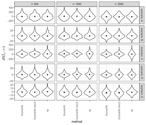
Figure 2: Sampling distribution of the scaled difference between MSE estimators and the true MSE in the four scenarios under concept shift in the features. The point stands for the empirical average in Monte Carlo simulations.

Figure 2 presents the sampling distribution of the scaled difference between the three estimators of the MSE and the true MSE. When Condition DS.1 holds, all three estimators appear close to normal and centered around the truth, demonstrating Theorem 2. The variance of Xconshift is much smaller than that of np in both Scenarios C and D for sample sizes 1000 and 2000, indicating a large efficiency gain; in the other two scenarios, the variance of these two estimators is comparable. These results are consistent with Corollary 3 and Remark 5. When Condition DS.1 does not hold (Scenario E), our proposed estimator appears consistent, indicating that $\hat{r}_{{\mathrm{Xcon}}}$ might be robust against moderate failures of the concept shift condition DS.1.

5 Full-data covariate shift

5.1 Efficiency bound

Let $g_{*}:x\mapsto P_{*}(A=0\mid X=x)$ be the propensity score function for the target population and $\mathcal{L}_{*}:x\mapsto\mathbb{E}_{P_{*}}[\ell(X,Y)\mid X=x]$ be the conditional risk function. Under Condition DS.3, $\mathcal{L}_{*}(x)=\mathbb{E}_{P_{*}}[\ell(X,Y)\mid X=x,A=0]=\mathbb{E}_{P_{*}}[\ell(X,Y)\mid X=x,A=1]$. For scalars $\rho\in(0,1)$, $r\in\real$ and functions $g,\mathcal{L}:\mathcal{X}\to\real$, define

$$D_{\mathrm{cov}}(\rho,g,\mathcal{L},r):o=(x,y,a)\mapsto\frac{g(x)}{\rho}\{\ell(x,y)-\mathcal{L}(x)\}+\frac{1-a}{\rho}\{\mathcal{L}(x)-r\}.$$ (17)

We have the following efficient influence function—implied by the efficiency bound under Condition DS.0 from (5)—as well as the associated relative efficiency gain.

Corollary 4.

Under Condition DS.3, if $g_{*}$ is bounded away from zero for almost every $x$ in the support of $X\mid A=0$, the efficient influence function for the risk $r_{*}$ is $D_{\mathrm{cov}}(\rho_{*},g_{*},\mathcal{L}_{*},r_{*})$. Thus, the smallest possible limiting normalized asymptotic variance for a sequence of RAL estimators is $\sigma_{*,{\mathrm{cov}}}^{2}:=\mathbb{E}_{P_{*}}[D_{\mathrm{cov}}$ $(\rho_{*},g_{*}$, $\mathcal{L}_{*},r_{*})(O)^{2}]$.

Corollary 5.

Under conditions of Corollary 4, the relative efficiency gain from using an efficient estimator is

$$1-\frac{\sigma_{*,{\mathrm{cov}}}^{2}}{\sigma_{*,{\mathrm{np}}}^{2}}=\frac{\mathbb{E}\left[g_{*}(X)(1-g_{*}(X))\mathbb{E}_{P_{*}}\left[\{\ell(X,Y)-\mathcal{L}_{*}(X)\}^{2}\mid X\right]\right]}{\mathbb{E}_{P_{*}}\left[g_{*}(X)\mathbb{E}_{P_{*}}[\{\ell(X,Y)-\mathcal{L}_{*}(X)\}^{2}\mid X]\right]+\mathbb{E}_{P_{*}}\left[g_{*}(X)\{\mathcal{L}_{*}(X)-r_{*}\}^{2}\right]}.$$

By Corollary 5, more efficiency gain is achieved for $P_{*}$ when the followings hold:

1. The propensity score $g_{*}$ is close to zero. If the covariate distribution in the source population covers that in the target population, then the proportion of source data is large.

2. The proportion of variance of $\ell(X,Y)$ not due to $X$ is large compared to that due to $X$.

The second property is the opposite of the implication of Corollary 3 under concept shift in the features. Therefore, in the illustrating example in Remark 5, the efficiency gain under covariate shift would be large if the given predictor $f$ is close to the oracle predictor $\mu_{*}$.

5.2 Cross-fit risk estimator

We propose to use a cross-fit estimator based on estimating equations, as described in Algorithm 3. This algorithm is the special case of Algorithm 1 with simplifications implied by Condition DS.3.

Algorithm 3 Cross-fit estimator of risk $r_{*}$ under full-data covariate shift condition DS.3

1:Randomly split all data (from both populations) into $V$ folds. Let $I_{v}$ be the indices of for fold $v$.

2:for $v\in[V]$ do Estimate $(g_{*},\mathcal{L}_{*})$ by $(\hat{g}^{-v},\hat{\mathcal{L}}^{-v})$ using data out of fold $v$.  

3:for $v\in[V]$ do $\triangleright$ (Obtain an estimating-equation-based estimator for fold $v$)

4:     With $\hat{\rho}^{v}:=\frac{1}{|I_{v}|}\sum_{i\in I_{v}}{\mathbbm{1}}(A_{i}=0)$, set

$$\hat{r}_{{\mathrm{cov}}}^{v}:=\frac{1}{\hat{\rho}^{v}|I_{v}|}\sum_{i\in I_{v}}\{\hat{g}^{-v}(X_{i})[\ell(X_{i},Y_{i})-\hat{\mathcal{L}}^{-v}(X_{i})]+{\mathbbm{1}}(A_{i}=0)\hat{\mathcal{L}}^{-v}(X_{i})\}.$$ (18)

5:Obtain the cross-fit estimator: $\hat{r}_{{\mathrm{cov}}}:=\frac{1}{n}\sum_{v=1}^{V}|I_{v}|\hat{r}_{{\mathrm{cov}}}^{v}$.

Compared to our proposed estimator $\hat{r}_{{\mathrm{Xcon}}}$ for concept shift, the estimator $\hat{r}_{{\mathrm{cov}}}$ involves two nuisance functions rather than one. As we will show next, in contrast to $\hat{r}_{{\mathrm{Xcon}}}$, the efficiency of $\hat{r}_{{\mathrm{cov}}}$ is based on sufficiently fast convergence rates—rather than consistency alone—of the nuisance function estimators, similarly to Theorem 1.

Condition ST.3 (Sufficient rate of convergence for nuisance estimators).

It holds that

$$\max_{v\in[V]}\left|\int(\hat{g}^{-v}-g_{*})(\hat{\mathcal{L}}^{-v}-\mathcal{L}_{*}){\mathrm{d}}P_{*}\right|={\mathrm{o}}_{p}(n^{-1/2}),$$

$$\max_{v\in[V]}\left\|\hat{g}^{-v}-g_{*}\right\|_{L^{2}(P_{*})}={\mathrm{o}}_{p}(1),\qquad\max_{v\in[V]}\left\|\hat{\mathcal{L}}^{-v}-\mathcal{L}_{*}\right\|_{L^{2}(P_{*})}={\mathrm{o}}_{p}(1).$$

This condition implies Condition ST.1 under Condition DS.3; but is perhaps a bit more interpretable. This leads to the efficiency of $\hat{r}_{{\mathrm{cov}}}$, whose proof has the same spirit as part 1 of Theorem 1.

Corollary 6 (Efficiency of $\hat{r}_{{\mathrm{cov}}}$).

Under Conditions DS.3 and ST.3, the sequence of estimators $\hat{r}_{{\mathrm{cov}}}$ in Line 5 of Alg. 3 is regular and efficient: with $r_{*}$ from (1) and $D_{{\mathrm{cov}}}$ from (17),

$$\hat{r}_{{\mathrm{cov}}}=r_{*}+\frac{1}{n}\sum_{i=1}^{n}D_{{\mathrm{cov}}}(\rho_{*},g_{*},\mathcal{L}_{*},r_{*})(O_{i})+{\mathrm{o}}_{p}(n^{-1/2}).$$

Therefore, with $\sigma_{*,{\mathrm{cov}}}^{2}$ from (4), $\sqrt{n}(\hat{r}_{{\mathrm{cov}}}-r_{*})\overset{d}{\to}\mathrm{N}(0,\sigma_{*,{\mathrm{cov}}}^{2})$.

Another difference between $\hat{r}_{{\mathrm{cov}}}$ and $\hat{r}_{{\mathrm{Xcon}}}$ is that $\hat{r}_{{\mathrm{cov}}}$ is doubly robust consistent, as implied by part 2 of Theorem 1, but not fully robust asymptotically linear. The doubly robust consistency of $\hat{r}_{{\mathrm{cov}}}$ relies on the following condition that corresponds to Condition ST.2 for sequential conditionals and is weaker than Condition ST.3. The comparison between these conditions is similar to that between Conditions ST.1 and ST.2.

Condition ST.4 (Consistent estimation of one nuisance function).

It holds that

$$\max_{v\in[V]}\left|\int(\hat{g}^{-v}-g_{*})(\hat{\mathcal{L}}^{-v}-\mathcal{L}_{*}){\mathrm{d}}P_{*}\right|={\mathrm{o}}_{p}(1),$$

$$\max_{v\in[V]}\left\|\hat{g}^{-v}-g_{*}\right\|_{L^{2}(P_{*})}={\mathrm{O}}_{p}(1),\qquad\max_{v\in[V]}\left\|\hat{\mathcal{L}}^{-v}-\mathcal{L}_{*}\right\|_{L^{2}(P_{*})}={\mathrm{O}}_{p}(1).$$

We obtain the doubly robust consistency for $\hat{r}_{{\mathrm{cov}}}$, a corollary of part 2 of Theorem 1.

Corollary 7 (Double robustness of $\hat{r}_{{\mathrm{cov}}}$).

Under Conditions DS.3 and ST.3, with $r_{*}$ from (1), the sequence of estimators $\hat{r}_{{\mathrm{cov}}}$ from Line 5 of Alg. 3 is consistent for $r_{*}$.

The differences between the asymptotic properties of $\hat{r}_{{\mathrm{Xcon}}}$ and $\hat{r}_{{\mathrm{cov}}}$ are due to the differences between the dataset shift conditions. Covariate shift DS.3 is independence conditional on covariates, while concept shift DS.1 is marginal independence. One aspect in which they differ is that conditional independence is often more difficult to test than marginal independence (Shah and Peters, 2020).

When covariate shift DS.3 holds, compared to the nonparametric estimator $\hat{r}_{{\mathrm{np}}}$, our proposed estimator $\hat{r}_{{\mathrm{cov}}}$ has advantages and limitations. In terms of efficiency, $\hat{r}_{{\mathrm{cov}}}$ may achieve efficiency gains when both nuisance functions are estimated consistently. In terms of robustness, $\hat{r}_{{\mathrm{np}}}$ does not require estimating any nuisance function and is therefore fully robust asymptotically linear; in contrast, $\hat{r}_{{\mathrm{cov}}}$ is only doubly robust consistent but not fully robust. A natural question is whether there exists a regular estimator that is fully robust asymptotically linear and also attains the efficiency bound under reasonable conditions, similarly to $\hat{r}_{{\mathrm{Xcon}}}$ under concept shift. Unfortunately, as the following result shows, such estimators do not exist under the common parametrizations $(P_{X},P_{A\mid X},P_{Y\mid X})$ and $(P_{A},P_{X\mid A},P_{Y\mid X})$ of the distribution $P$.

Lemma 1.

Suppose that the covariate shift condition DS.3 holds, but no further assumptions on $P_{*}$ are made. Under the parametrization $(P_{X},P_{A\mid X},P_{Y\mid X})$ of a distribution $P$, suppose that for all $P_{*}$, ${\mathrm{IF}}(P_{*,X},$ $P_{A\mid X},P_{Y\mid X},r_{*})$ is an influence function for estimating $r_{*}$ at $P_{*}$, for arbitrary $(P_{A\mid X},P_{Y\mid X})$. Then, we have that

$${\mathrm{IF}}(P_{*,X},P_{A\mid X},P_{Y\mid X},r_{*})=D_{\mathrm{np}}(\rho_{*},r_{*}).$$

A similar result holds under the parametrization $(P_{A},P_{X\mid A},P_{Y\mid X})$ of $P$.

Therefore, if a regular estimator of $r_{*}$ is fully robust asymptotically linear under either of the above parametrizations, that is, its influence function satisfies the assumptions for ${\mathrm{IF}}$ in either case of Lemma 1, then its influence function must be $D_{\mathrm{np}}(\rho_{*},r_{*})$ and cannot attain the efficiency bound. Since full-data covariate shift (DS.3) under the second parametrization in the above lemma is a special case of Condition DS.0 under the common parametrization $(P_{A},P_{Z_{1}\mid A},\ldots,P_{Z_{K}\mid\bar{Z}_{K-1},A})$ of distributions $P$ (Li and Luedtke, 2023), we also conclude that there is generally no regular and fully robust asymptotically linear estimator of $r_{*}$ that can attain the efficiency bound for Condition DS.0 under this parametrization.

We ran a simulation similar to that in Section 4.3. The results, which are presented in Supplement S5, demonstrate our theoretical results about the efficiency gains and the asymptotic behavior of our proposed estimator $\hat{r}_{\mathrm{cov}}$.

6 Other dataset shift conditions

In addition to the four dataset shift conditions DS.1–DS.4, we study a few other classes of conditions from prior work that are model-agnostic and lead to semiparametric models. For all these conditions, data $Z$ consists of covariate/feature $X$ and outcome/label $Y$; only one source population is present, and so the population indicator $A$ is binary. In each following subsection, we first present a condition and then characterize semiparametric efficiency bounds under this condition.

6.1 Posterior drift conditions

Scott (2019) introduced two similar conditions for a binary label $Y\in\{0,1\}$. The more general one is the following covariate shift posterior drift.

Condition DS.5 (Covariate Shift Posterior Drift).

There exists an unknown differentiable function $\tilde{\phi}_{*}$ such that for all $x$,

$$P_{*}(Y=1\mid X=x,A=1)=\tilde{\phi}_{*}\left(P_{*}(Y=1\mid X=x,A=0)\right),$$ (19)

$$\left.\frac{{\mathrm{d}}\tilde{\phi}_{*}(\theta)}{{\mathrm{d}}\theta}\right|_{\theta=P_{*}(Y=1\mid X=x,A=0)}\neq 0$$

As usual, in the above notations, the subscript $*$ stands for the true data-generating distribution $P_{*}$. We have slightly modified the original condition in Scott (2019); see Supplement S6 for more details. Condition DS.5 models labeling errors in the training data ($A=1$). In general, in the source population data where objects are manually labeled, labeling errors may occur, and these errors are often related to the true label in such a way that, given any object with a high probability of having the true label being one, humans are also likely to label it as one. As shown in Section 3 of Scott (2019), Condition DS.5 is implied by label shift (DS.4).

We have the following results on the efficient influence function for estimating $r_{*}$ under Condition DS.5.

Theorem 3.

Recall $\rho_{*}:=P_{*}(A=0)$ and $\mathcal{E}_{*}:x\mapsto\mathbb{E}_{P_{*}}[\ell(X,Y)\mid X=x,A=0]$. For any functions $f_{1},f_{2}\in L^{2}(P_{*,X})$, define

$$\theta_{*}(x) :=\operatorname{logit}P_{*}(A=1\mid X=x),$$

$$F(f_{1},f_{2}) :o\mapsto a\left\{y-\operatorname{expit}\circ\phi_{*}\circ\theta_{*}(x)\right\}f_{1}(x)+(1-a)\left\{y-\operatorname{expit}\circ\theta_{*}(x)\right\}f_{2}(x),$$

$$v(x;a) :={\mathrm{var}}_{P_{*}}(Y\mid A=a,X=x)P_{*}(A=a\mid X=x),$$

$$\kappa(x) :=\frac{v(x;0)\mathbb{E}[v(X;1)\mid\theta_{*}(X)=\theta_{*}(x)]}{v(x;1)\{\phi^{\prime}\circ\theta_{*}(x)\}^{2}}\frac{\ell(x,1)-\ell(x,0)}{\rho_{*}},$$

$$\mu(x) :=\mathbb{E}[v(X;1)\mid\theta_{*}(X)=\theta_{*}(x)]\left\{1+\frac{v(x;0)}{v(x;1)\{\phi^{\prime}\circ\theta_{*}(x)\}^{2}}\right\}.$$

Let $\mathscr{A}$ be the linear integral operator such that, for any function $g\in L^{2}(P_{*,X})$,

$$\mathscr{A}g(x)=\mathbb{E}_{P_{*}}\left[g(X)\frac{v(X;1)}{\mu(X)}\mid\theta_{*}(X)=\theta_{*}(x)\right].$$

Suppose that the following Fredholm integral equation of the second kind (see, e.g., Kress, 2014) for unknown $\zeta:\mathcal{X}\to\real$ has a unique solution $\zeta_{*}$:

$$\mathscr{A}\zeta+\kappa=\zeta.$$ (20)

Let $g_{1}:x\mapsto-\mathscr{A}\zeta_{*}(x)\cdot\phi_{*}^{\prime}\circ\theta_{*}(x)/\mathscr{A}\mu(x)+\phi_{*}^{\prime}\circ\theta_{*}(x)\cdot\zeta_{*}/\mu$ and $g_{2}:=\zeta_{*}/\mu$. Under Condition DS.5, the efficient influence function for estimating $r_{*}$ is $D_{\mathrm{cspd}}:o\mapsto(1-a)\left\{\mathcal{E}_{*}(x)-r_{*}\right\}/\rho_{*}+F(g_{1},g_{2})(o)$.

The existence and uniqueness of the solution to (20) can be shown using, for example, Theorem 2.14 or Corollary 3.5 of Kress (2014).

The other dataset shift condition in Scott (2019), posterior drift, is similar to Condition DS.5. We present the corresponding results in Supplement S6.

6.2 Location-scale shift conditions

Zhang et al. (2013) introduced two dataset shift conditions for vector-valued covariates $X\in{}^{d}$. The more general condition is location-scale generalized target shift.

Condition DS.6 (Location-Scale Generalized Target Shift).

There exists an unknown function $W_{*}:\mathcal{Y}\to{}^{d\times d}$ whose values are invertible matrices, and an unknown function $b_{*}:\mathcal{Y}\to{}^{d}$ such that, for all $y\in\mathcal{Y}$,

$$W_{*}(Y)X+b_{*}(Y)\mid Y=y,A=1\quad\text{and}\quad X\mid Y=y,A=0$$

are identically distributed.

Condition DS.6 imposes a specific form on the relationship between the two distributions $X\mid Y,A=1$ and $X\mid Y,A=0$, a location-scale shift, and is thus more general than label shift (DS.4). We have also slightly modified the original condition in Zhang et al. (2013); see Supplement S6.

We next present the results on the efficient influence function for estimating $r_{*}$ under the above conditions. For any differentiable function $f:{}^{d}\to\real$, let $\partial_{i}$ denote partial differentiation with respect to the $i$-th variable, and let $f^{\prime}$ or $\partial f(x)/\partial x$ denote the gradient of $f$. Let $v_{i}$ denote the $i$-the entry of a vector $v$, $I_{d\times d}$ be the ^d×d-identity matrix, and $1_{d}$ be the ^d-vector of ones.

Theorem 4.

Suppose that the distribution of $X\mid A=a,Y=y$ has a differentiable Lebesgue density supported on ^d for all $a\in\{0,1\}$ and $y\in\mathcal{Y}$. Recall $\rho_{*}:=P_{*}(A=0)$, $g_{*,Y}:y\mapsto P_{*}(A=0\mid Y=y)$ and $\mathcal{E}_{*,Y}:y\mapsto\mathbb{E}_{P_{*}}[\ell(X,Y)\mid Y=y,A=0]$. Let $\tau_{*}(x\mid y)$ be the Lebesgue density of $X\mid A=0,Y=y$ under $P_{*}$, and define

$$\psi_{y}(x) :=W_{*}(y)x+b_{*}(y),\qquad\Phi(x,y):=\left\{\ell(x,y)-\mathcal{E}_{*,Y}(y)\right\}/\rho_{*},$$

$$\Gamma(x,y) :=(x-b_{*}(y))\cdot\partial_{1}\log\tau_{*}(x\mid y),\quad\Lambda(x,y):=I_{d\times d}+(x-b_{*}(y))\{(\log\tau_{*})^{\prime}(x\mid y)\}^{\top},$$

$$a(y) :=\begin{pmatrix}\mathbb{E}_{P_{*}}\left[\Phi(X,Y)\left\{1+\Gamma(X,Y)\right\}\mid A=0,Y=y\right]\\ \mathbb{E}\left[\Phi(X,Y)\cdot\partial_{1}\log\tau_{*}(X\mid Y)\mid A=0,Y=y\right]\end{pmatrix},$$

$$M_{11}(y) :=\mathbb{E}_{P_{*}}\Big{[}\operatorname{tr}\left(W_{*}(Y)^{-1}\Lambda(X,Y)\right)\cdot\left\{1+\Gamma(X,Y)\right\}\mid A=0,Y=y\Big{]},$$

$$M_{12}(y) :=\mathbb{E}_{P_{*}}\Big{[}\{(\log\tau_{*})^{\prime}(X\mid Y)\}^{\top}1_{d}\cdot\left\{1+\Gamma(X,Y)(X_{1}-b_{*,1}(Y))\right\}\mid A=0,Y=y\Big{]},$$

$$M_{21}(y) :=\mathbb{E}_{P_{*}}\Big{[}\operatorname{tr}\left(W_{*}(Y)^{-1}\Lambda(X,Y)\right)\cdot\partial_{1}\log\tau_{*}(X\mid Y)\mid A=0,Y=y\Big{]},$$

$$M_{22}(y) :=\mathbb{E}_{P_{*}}\left[\{(\log\tau_{*})^{\prime}(X\mid Y)\}^{\top}1_{d}\cdot\partial_{1}\log\tau_{*}(X\mid Y)\mid A=0,Y=y\right],$$

$$M(y) :=\begin{pmatrix}M_{11}(y)&M_{12}(y)\\ M_{21}(y)&M_{22}(y)\end{pmatrix},\qquad c(x,y):=\begin{pmatrix}\operatorname{tr}\left(W_{*}(y)^{-1}\Lambda(x,y)\right)\\ \{(\log\tau_{*})^{\prime}(x\mid y)\}^{\top}1_{d}\end{pmatrix},$$

$$N(o) :=(1-a)\left\{(g_{*,Y}(y))\Phi(x,y)-(1-g_{*,Y}(y))c(x,y)^{\top}M(y)^{-1}a(y)\right\}$$

$$\quad+ag_{*,Y}(y)\left\{\Phi(\psi_{y}(x),y)+c(\psi_{y}(x),y)M(y)^{-1}a(y)\right\}.$$

Under Condition DS.6, the efficient influence function for estimating $r_{*}$ is $D_{\mathrm{lsgts}}:o\mapsto(1-a)\left\{\mathcal{E}_{*,Y}(y)-r_{*}\right\}/\rho_{*}+N(o)$.

Zhang et al. (2013) introduced another similar dataset shift condition, location-scale conditional shift. We present the corresponding results in Supplement S6.

7 Discussion

Under covariate shift (DS.3), it is possible to construct a doubly robust asymptotically linear—rather than just consistent—estimator that is efficient when both nuisance functions are estimated consistently. However, when one nuisance function estimator is not consistent, such an estimator might no longer be regular, potentially resulting in undesirable finite-sample performance for some data-generating distributions and nuisance function estimators (see, e.g., Dukes et al., 2021). The above discussion might also apply to the more general dataset shift condition DS.0.

We have derived the efficiency bound for several challenging dataset shift conditions in Section 6. The efficient influence functions under these semiparametric models are hardly tractable, and constructing efficient estimators by solving an estimating equation currently appears infeasible in practice. To overcome this challenge, it might be of future interest to develop reliable methods to construct efficient estimators that require little knowledge about efficient influence functions, for example, methods proposed by Carone et al. (2019).

In this paper, we study domain adaptation under dataset shift conditions through the lens of semiparametric efficiency theory and have developed efficient and robust risk estimators for common dataset shift conditions. Our results may inspire future research on domain adaptation methods with more desirable properties.

S1 Further examples of sequential conditionals

We provide here some further examples of models satisfying the sequential conditionals condition (Condition DS.0).

Example S1 (Covariate & concept shift).

Suppose that $Z=(X,Y)$ and in addition to a fully observed dataset from the target population ($A=0$), two source datasets are available: one dataset ($A=1$) contains unlabeled data—that is, $Y$ is missing—from the target population; the other ($A=2$) contains fully observed data from a relevant source population satisfying covariate shift. For example, an investigator might wish to train a prediction model in a new target population with little data. The investigator might start collecting unlabeled data from the target population, label some target population data, and further leverage a large existing source data set that was assembled for a similar prediction task. Condition DS.0 reduces to this setup with $K=2$, $\mathcal{A}=\{0,1,2\}$, $Z_{1}=X$, $Z_{2}=Y$, $\mathcal{S}_{1}=\{1\}$ and $\mathcal{S}_{2}=\{2\}$.

Example S2 (Multiphase sampling).

Suppose that we have variables $Z_{K}$ that are expensive to measure (e.g., personal interview responses, thorough diagnostic evaluation, or manual field measurements) and relatively inexpensive variables $\bar{Z}_{K-1}$ (e.g., mail survey responses, screening instruments, or sensor measurements). The investigator might draw a random sample from the target population measuring the inexpensive variables, but only measure $Z_{K}$ for a random subsample. We label the subsample of full datapoints with $A=0$, and label subsamples of incomplete observations with other indices in $\mathcal{A}$.

It might be reasonable to assume Condition DS.0, stating that the distributions of $Z_{K}|\bar{Z}_{K-1},A=0$ and $Z_{K}|\bar{Z}_{K-1},A=a$ are identical for $a\in\mathcal{S}_{k}$ for some index set $\mathcal{S}_{k}$. This setup can arise from a two-phase sampling design (e.g., Hansen and Hurwitz, 1946; Shrout and Newman, 1989, etc.) for $K=2$, or multiphase sampling (e.g. Srinath, 1971; Tuominen et al., 2006, etc.) for larger $K$.

S2 General sequential conditionals

As mentioned in Remark 4, in this section, we study a dataset shift condition that is more general than Condition DS.0 for transfer learning. This condition was introduced by Li and Luedtke (2023) with applications to data fusion and causal inference. Let $Q$ denote the target population so that the target estimand, the target population risk, is $\mathbb{E}_{Q}[\ell(Z)]$.

In contrast to the setting from the main text, we do not assume that data drawn from $Q$ is observed; our results hold regardless if there is any data observed from $Q$. Thus, we allow the index set $\mathcal{A}$ not to contain zero, the index for the target population. This condition is useful if fully observed data from the target population $Q$ is unavailable, but information about conditional distributions under $Q$ can be learned from source populations; therefore, transfer learning is still viable. We will show that, under this more general condition, we can still construct an efficient and multiply robust estimator of $\mathbb{E}_{Q}[\ell(Z)]$ under conditions similar to those from Section 3. However, due to a lack of data from the target population, we might not be able to test whether our estimator is consistent for the estimand $\mathbb{E}_{Q}[\ell(Z)]$ of interest.

We will use notations similar to those from Section 3. The more general dataset shift condition is the following.

Condition DS.S0 (General sequential conditionals).

For every $k\in[K]$, there exists a known nonempty subset $\mathcal{S}^{\prime}_{k}\subset\mathcal{A}$ such that, for all $a\in\mathcal{S}^{\prime}_{k}$, $Z_{k}\mid\bar{Z}_{k-1}=\bar{z}_{k-1},A=a$ is distributed identically to $Z_{k}\mid\bar{Z}_{k-1}=\bar{z}_{k-1}$ under $Q$ for $Q$-almost every $\bar{z}_{k-1}$ in the support $\widetilde{\mathcal{Z}}_{k-1}$ of $\bar{Z}_{k-1}$ under $Q$.

We also assume that the distribution of $\bar{Z}_{k-1}$ under $Q$ is dominated by $\bar{Z}_{k-1}\mid A\in\mathcal{S}^{\prime}_{k}$ under $P_{*}$ throughout this section. Then the above condition reduces to Condition DS.0 if $0\in\mathcal{A}$ and $0\in\mathcal{S}^{\prime}_{k}$ for all $k\in[K]$, and $Q=P_{*}(\cdot|A=0)$. For this dataset shift condition, we define recursively $\ell^{K}_{*}:=\ell$ and

$$\ell^{k}_{*}:\bar{z}_{k}\mapsto\mathbb{E}_{P_{*}}[\ell^{k+1}_{*}(\bar{Z}_{k+1})\mid\bar{Z}_{k}=\bar{z}_{k},A\in\mathcal{S}^{\prime}_{k+1}]\ \ \text{for }\bar{z}_{k}\in\widetilde{\mathcal{Z}}_{k},\ k\in[K-1].$$ (S1)

We also denote $r_{*}=\mathbb{E}_{Q}[\ell(Z)]$. We allow $\ell^{k}_{*}$ to take any value outside $\widetilde{\mathcal{Z}}_{k}$. These functions are identical to the functions $\ell^{k}_{*}$ defined in Section 3 under Condition DS.0; otherwise, they may differ. Let $\bm{\ell}_{*}:=(\ell^{k}_{*})_{k=1}^{K-1}$. We use $\lambda^{k-1}_{*}$ to denote the Radon-Nikodym derivative of the distribution of $\bar{Z}_{k-1}$ under $Q$ relative to that of $\bar{Z}_{k-1}\mid A\in\mathcal{S}^{\prime}_{k}$ under $P_{*}$. Under the stronger condition DS.0, it follows from Bayes’ Theorem that

$$\lambda^{k-1}_{*}=\frac{\sum_{a\in\mathcal{S}^{\prime}_{k}}\pi^{a}_{*}}{\pi^{0}_{*}(1+\theta^{k-1}_{*})}$$ (S2)

with $\pi^{0}_{\star}$ and $\theta_{\star}^{k}$ defined in Section 3. We use $\bm{\lambda}_{*}$ to denote the collection $(\lambda^{k}_{*})_{k=1}^{K-1}$; since $\lambda^{0}_{*}=1$ is a constant, we have dropped it from $\bm{\lambda}_{*}$. For any collections $\bm{\ell}$, $\bm{\lambda}$, and $\bm{\pi}$ of nuisances, define the pseudo-loss

$$\widetilde{\mathcal{T}}(\bm{\ell},\bm{\lambda},\bm{\pi}):o=(z,a)\mapsto\sum_{k=2}^{K}\frac{{\mathbbm{1}}(a\in\mathcal{S}^{\prime}_{k})}{\sum_{b\in\mathcal{S}^{\prime}_{k}}\pi^{b}}\lambda^{k-1}(\bar{z}_{k-1})[\ell^{k}(\bar{z}_{k})-\ell^{k-1}(\bar{z}_{k-1})]+\frac{{\mathbbm{1}}(a\in\mathcal{S}^{\prime}_{1})}{\sum_{b\in\mathcal{S}^{\prime}_{1}}\pi^{b}}\ell^{1}(\bar{z}_{1})$$ (S3)

and, given also any scalar $r$, define

$$D_{\mathrm{GSC}}(\bm{\ell},\bm{\lambda},\bm{\pi},r):o=(z,a)\mapsto\widetilde{\mathcal{T}}(\bm{\ell},\bm{\lambda},\bm{\pi})(o)-\frac{{\mathbbm{1}}(a\in\mathcal{S}^{\prime}_{1})}{\sum_{b\in\mathcal{S}^{\prime}_{1}}\pi^{b}}r,$$ (S4)

where $\ell^{K}:=\ell$. We have the following efficiency bound for estimating $r_{*}$, which is implied by Theorem 2 and Corollary 1 in Li and Luedtke (2023).

Corollary S1.

Under Condition DS.S0, if for all $k\in[K]$, $\lambda^{k-1}_{*}(\bar{z}_{k-1})$ is uniformly bounded away from zero and infinity as a function of $\bar{z}_{k-1}\in\widetilde{\mathcal{Z}}_{k-1}$, then the efficient influence function for estimating $r_{*}$ at $P_{*}$ is $D_{\mathrm{GSC}}(\bm{\ell}_{*},\bm{\lambda}_{*},\bm{\pi}_{*},r_{*})$.

Algorithm S1 Cross-fit estimator of $r_{*}=\mathbb{E}_{Q}[\ell(Z)]$ under Condition DS.S0

1:Split data as in Line 1, Algorithm 1.

2:for $v\in[V]$ do

3:     For all $k=1,\ldots,K-1$, estimate $\lambda^{k}_{*}$ by $\hat{\lambda}^{k}_{v}$ using data out of fold $v$. Set $\widehat{\bm{\lambda}}_{v}:=(\hat{\lambda}^{k}_{v})_{k=1}^{K-1}$.

4:     Set $\hat{\pi}^{a}_{v}:=|I_{v}|^{-1}\sum_{i\in I_{v}}{\mathbbm{1}}(A_{i}=a)$ for all $a\in\mathcal{A}$, $\widehat{\bm{\pi}}_{v}:=(\hat{\pi}^{a}_{v})_{a\in\mathcal{A}}$, and $\hat{\ell}^{K}_{v}$ to be $\ell$.

5:     for $k=K-1,\ldots,1$ do

6:         Estimate $\ell^{k}_{*}$ by $\hat{\ell}^{k}_{v}$ as in Line 6, Algorithm 1.      

7:     Set $\widehat{\bm{\ell}}_{v}:=(\hat{\ell}^{k}_{v})_{k=1}^{K-1}$.

8:     Compute the following estimator for fold $v$:

$$\hat{r}_{v}:=\frac{1}{|I_{v}|}\sum_{i\in I_{v}}\widetilde{\mathcal{T}}(\widehat{\bm{\ell}}_{v},\widehat{\bm{\lambda}}_{v},\widehat{\bm{\pi}}_{v})(O_{i}).$$ (S5)

9:Compute the cross-fit estimator combining estimators $\hat{r}_{v}$ from all folds:

$$\hat{r}:=\frac{1}{n}\sum_{v=1}^{V}|I_{v}|\hat{r}_{v}.$$ (S6)

We propose to use the cross-fit estimator $\hat{r}$ from Algorithm S1 to estimate $r_{*}$. Algorithm 1 is a special case of Algorithm S1 under Condition DS.0. We next present conditions for the efficiency and multiple robustness of $\hat{r}$. These conditions are counterparts of Conditions ST.1 and ST.2 corresponding to the more general condition DS.S0. For all $k\in[2:K]$, define

$$B_{k} =\left(\sum_{a\in\mathcal{S}^{\prime}_{1}}\hat{\pi}^{a}_{v}\right)\frac{\sum_{a\in\mathcal{S}^{\prime}_{k}}\pi^{a}_{*}}{\sum_{a\in\mathcal{S}^{\prime}_{k}}\hat{\pi}^{a}_{v}}\mathbb{E}_{P_{*}}\Bigg{[}\left\{\hat{\lambda}^{k-1}_{v}(\bar{Z}_{k-1})-\lambda^{k-1}_{*}(\bar{Z}_{k-1})\right\}$$ (S7)

$$\qquad\qquad\times\left\{\mathbb{E}_{P_{*}}\left[\hat{\ell}^{k}_{v}(\bar{Z}_{k})\mid\bar{Z}_{k-1},A\in\mathcal{S}^{\prime}_{k}\right]-\hat{\ell}^{k-1}_{v}(\bar{Z}_{k-1})\right\}\mid A\in\mathcal{S}^{\prime}_{k}\Bigg{]}$$

$$\quad+\left\{\left(\sum_{a\in\mathcal{S}^{\prime}_{1}}\hat{\pi}^{a}_{v}\right)\frac{\sum_{a\in\mathcal{S}^{\prime}_{k}}\pi^{a}_{*}}{\sum_{a\in\mathcal{S}^{\prime}_{k}}\hat{\pi}^{a}_{v}}-\sum_{a\in\mathcal{S}^{\prime}_{1}}\pi^{a}_{*}\right\}\mathbb{E}_{Q}\left[\mathbb{E}_{P_{*}}\left[\hat{\ell}^{k}_{v}(\bar{Z}_{k})\mid\bar{Z}_{k-1},A\in\mathcal{S}^{\prime}_{k}\right]-\hat{\ell}^{k-1}_{v}(\bar{Z}_{k-1})\right].$$

Condition ST.S1.

For every fold $v\in[V]$,

1. the following term is ${\mathrm{o}}_{p}(n^{-1/2})$:

   $$\begin{split}&\sum_{k=2}^{K}B_{k};\end{split}$$ (S8)

2. the following term is ${\mathrm{o}}_{p}(1)$:

   $$\left\|\left(\sum_{a\in\mathcal{S}^{\prime}_{1}}\hat{\pi}^{a}_{v}\right)\widetilde{\mathcal{T}}(\widehat{\bm{\ell}}_{v},\widehat{\bm{\lambda}}_{v},\widehat{\bm{\pi}}_{v})-\left(\sum_{a\in\mathcal{S}^{\prime}_{1}}\pi^{a}_{*}\right)\widetilde{\mathcal{T}}(\bm{\ell}_{*},\bm{\lambda}_{*},\bm{\pi}_{*})\right\|_{L^{2}(P_{*})}.$$ (S9)

Condition ST.S2.

For all $v\in[V]$, (S8) is ${\mathrm{o}}_{p}(1)$ and (S9) is ${\mathrm{O}}_{p}(1)$.

Under the stronger Condition DS.0, Conditions ST.S1 and ST.S2 reduce to Conditions ST.1 and ST.2, respectively, with the nuisance estimator $\hat{\lambda}^{k-1}_{v}$ being $\sum_{a\in\mathcal{S}^{\prime}_{k}}\hat{\pi}^{a}_{v}/\{\hat{\pi}^{0}_{v}(1+\hat{\theta}^{k-1}_{v})\}$. The latter is a natural estimator of $\lambda^{k-1}_{*}$ using the parametrization from Section 3, in view of (S2).

Theorem S1.

With nuisance estimators $\widehat{\bm{\ell}}_{v}$, $\widehat{\bm{\lambda}}^{k}_{v}$ and $\widehat{\bm{\pi}}_{v}$ from Algorithm S1, define

$$\tilde{\Delta}_{v}:=\frac{\sum_{a\in\mathcal{S}^{\prime}_{1}}\pi^{a}_{*}}{\sum_{a\in\mathcal{S}^{\prime}_{1}}\hat{\pi}^{a}_{v}}\sum_{k=1}^{K}\mathbb{E}_{Q}\left[\mathbb{E}_{P_{*}}\left[\hat{\ell}^{k}_{v}(\bar{Z}_{k})\mid\bar{Z}_{k-1},A\in\mathcal{S}^{\prime}_{k}\right]-\hat{\ell}^{k}_{v}(\bar{Z}_{k})\right]$$ (S10)

for every fold $v\in[V]$ and

$$\tilde{\Delta}:=\frac{1}{n}\sum_{v=1}^{V}|I_{v}|\tilde{\Delta}_{v}.$$

1. Efficiency: Under Condition ST.S1, with $\hat{r}$ from (S6) and $D_{\mathrm{GSC}}$ in (S4), it holds that

   $$\hat{r}-\tilde{\Delta}=r_{*}+\frac{1}{n}\sum_{i=1}^{n}D_{\mathrm{GSC}}(\bm{\ell}_{*},\bm{\lambda}_{*},\bm{\pi}_{*},r_{*})(O_{i})+{\mathrm{o}}_{p}(n^{-1/2}).$$ (S11)

   Additionally under Condition DS.S0, $\tilde{\Delta}=0$ and thus $\hat{r}$ is regular and efficient.

2. Multiply robust consistency: Under Condition ST.S2, $\hat{r}-\tilde{\Delta}\overset{p}{\to}r_{*}$ as $n\to\infty$. Additionally, under Condition DS.S0, $\tilde{\Delta}=0$ and thus $\hat{r}$ is consistent for $r_{*}$.

S3 Results for concept shift in the labels and full-data label shift

In this section, we present estimators and their theoretical properties for concept shift in the labels (DS.2) and full-data label shift (DS.4). Because of their similarity to Conditions DS.1 and DS.3, we abbreviate the presentation and omit the proofs of theoretical results. All theoretical results are numbered in parallel to those in the main text with a superscript $\dagger$.

S3.1 Concept shift in the labels

Define $\mathcal{E}_{*,Y}:y\mapsto\mathbb{E}_{P_{*}}[\ell(X,Y)\mid Y=y,A=0]$. For scalars $\rho\in(0,1)$, $r\in\real$, and a function $\mathcal{Y}:\mathcal{Y}\to\real$, define

$$D_{\mathrm{Ycon}}(\rho,\mathcal{E}_{Y},r):o=(x,y,a)\mapsto\frac{1-a}{\rho}\{\ell(x,y)-\mathcal{E}_{Y}(y)\}+\mathcal{E}_{Y}(y)-r.$$

Corollary 2^†.

Under Condition DS.2, the efficient influence function for the risk $r_{*}$ is $D_{\mathrm{Ycon}}(\rho_{*},\mathcal{E}_{*,Y},r_{*})$. Thus, the smallest possible normalized limiting variance for a sequence of RAL estimators is $\sigma_{*,{\mathrm{Ycon}}}^{2}:=\mathbb{E}_{P_{*}}[D_{\mathrm{Ycon}}(\rho_{*},\mathcal{E}_{*,Y},r_{*})(O)^{2}]$.

Corollary 3^†.

Under Condition DS.2, the relative efficiency gain from using an efficient estimator is

$$1-\frac{\sigma_{*,{\mathrm{Ycon}}}^{2}}{\sigma_{*,{\mathrm{np}}}^{2}}=\frac{(1-\rho_{*})\mathbb{E}_{P_{*}}\left[(\mathcal{E}_{*,Y}(y)-r_{*})^{2}\right]}{\mathbb{E}_{P_{*}}\left[\mathbb{E}_{P_{*}}\left[\{\ell(X,Y)-\mathcal{E}_{*,Y}(Y)\}^{2}\mid A=0,X\right]\right]+\mathbb{E}_{P_{*}}\left[\{\mathcal{E}_{*,Y}(Y)-r_{*}\}^{2}\right]}.$$

Our proposed estimator is described in Algorithm 2^†.

Algorithm 2^† Cross-fit estimator of risk $r_{*}$ under Condition DS.2, concept shift in the labels

1:Randomly split all data (from both populations) into $V$ folds. Let $I_{v}$ be the indices of data points in fold $v$.

2:for $v\in[V]$ do Estimate $\mathcal{E}_{*,Y}$ by $\hat{\mathcal{E}}_{Y}^{-v}$ using data out of fold $v$.  

3:for $v\in[V]$ do $\triangleright$ (Obtain an estimating-equation-based estimator for fold $v$)

4:     With $\hat{\rho}^{v}:=\frac{1}{|I_{v}|}\sum_{i\in I_{v}}{\mathbbm{1}}(A_{i}=0)$, set

$$\hat{r}_{{\mathrm{Ycon}}}^{v}:=\frac{1}{|I_{v}|}\sum_{i\in I_{v}}\left\{\frac{{\mathbbm{1}}(A_{i}=0)}{\hat{\rho}^{v}}[\ell(X_{i},Y_{i})-\hat{\mathcal{E}}_{Y}^{-v}(Y_{i})]+\hat{\mathcal{E}}_{Y}^{-v}(X_{i})\right\}.$$ (S12)

5:Obtain the cross-fit estimator:

$$\hat{r}_{{\mathrm{Ycon}}}:=\frac{1}{n}\sum_{v=1}^{V}|I_{v}|\hat{r}_{{\mathrm{Ycon}}}^{v}.$$ (S13)

Theorem 2^† (Efficiency and fully robust asymptotic linearity of $\hat{r}_{{\mathrm{Ycon}}}$).

Suppose that there exists a function $\mathcal{E}_{\infty,Y}:\mathcal{Y}\to\mathbb{R}$ such that

$$\max_{v\in[V]}\left\|\hat{\mathcal{E}}_{Y}^{-v}-\mathcal{E}_{\infty,Y}\right\|_{L^{2}(P_{*})}={\mathrm{o}}_{p}(1).$$

Under Condition DS.2, the estimator $\hat{r}_{{\mathrm{Ycon}}}$ in (S13) is RAL:

$$\hat{r}_{{\mathrm{Ycon}}}=r_{*}+\frac{1}{n}\sum_{i=1}^{n}\left\{D_{{\mathrm{Ycon}}}(\rho_{*},\mathcal{E}_{\infty,Y},r_{*})+\frac{\mathbb{E}_{P_{*}}\left[\mathcal{E}_{\infty,Y}(Y)\right]-r_{*}}{\rho_{*}}(1-A_{i}-\rho_{*})\right\}+{\mathrm{o}}_{p}(n^{-1/2}).$$

Moreover, if $\mathcal{E}_{*,Y}$ is estimated consistently, namely $\mathcal{E}_{\infty,Y}=\mathcal{E}_{*,Y}$, then $\hat{r}_{{\mathrm{Ycon}}}$ is asymptotically efficient:

$$\hat{r}_{{\mathrm{Ycon}}}=r_{*}+\frac{1}{n}\sum_{i=1}^{n}D_{{\mathrm{Ycon}}}(\rho_{*},\mathcal{E}_{*,Y},r_{*})(O_{i})+{\mathrm{o}}_{p}(n^{-1/2}).$$

S3.2 Full-data label shift

Define $g_{*,Y}:y\mapsto P_{*}(A=0\mid Y=y)$ and $\mathcal{L}_{*,Y}:y\mapsto\mathbb{E}_{P_{*}}[\ell(X,Y)\mid Y=y]$. For scalars $\rho\in(0,1)$, $r\in\real$ and functions $g_{Y},\mathcal{L}_{Y}:\mathcal{Y}\to\real$, define

$$D_{\mathrm{lab}}(\rho,g_{Y},\mathcal{L}_{Y},r):o=(x,y,a)\mapsto\frac{g_{Y}(y)}{\rho}\{\ell(x,y)-\mathcal{L}_{Y}(y)\}+\frac{1-a}{\rho}\{\mathcal{L}_{Y}(y)-r\}.$$

Corollary 4^†.

Under Condition DS.4, if $g_{*,Y}$ is bounded away from zero for almost every $x$ in the support of $Y\mid A=0$, the efficient influence function for the risk $r_{*}$ is $D_{\mathrm{lab}}(\rho_{*},g_{*,Y},\mathcal{L}_{*,Y},r_{*})$. Thus, the smallest possible limiting normalized variance for a sequence of RAL estimators is $\sigma_{*,{\mathrm{lab}}}^{2}:=\mathbb{E}_{P_{*}}[D_{\mathrm{lab}}(\rho_{*},g_{*,Y},\mathcal{L}_{*,Y},r_{*})(O)^{2}]$.

Corollary 5^†.

Under Condition DS.4, the relative efficiency gain from using an efficient estimator is

$$1-\frac{\sigma_{*,{\mathrm{lab}}}^{2}}{\sigma_{*,{\mathrm{np}}}^{2}}=\frac{\mathbb{E}_{P_{*}}\left[g_{*,Y}(Y)(1-g_{*,Y}(Y))\mathbb{E}_{P_{*}}\left[\{\ell(X,Y)-\mathcal{L}_{*,Y}(Y)\}^{2}\mid Y\right]\right]}{\mathbb{E}_{P_{*}}\left[g_{*,Y}(Y)\mathbb{E}_{P_{*}}[\{\ell(X,Y)-\mathcal{L}_{*,Y}(Y)\}^{2}\mid Y]\right]+\mathbb{E}_{P_{*}}\left[g_{*,Y}(Y)\{\mathcal{L}_{*,Y}(Y)-r_{*}\}^{2}\right]}.$$

Our proposed estimator is described in Algorithm 3^†.

Algorithm 3^† Cross-fit estimator of risk $r_{*}$ under full-data label shift condition DS.4

1:Randomly split all data (from both populations) into $V$ folds. Let $I_{v}$ be the indices of data points in fold $v$.

2:for $v\in[V]$ do Estimate $(g_{*,Y},\mathcal{L}_{*,Y})$ by $(\hat{g}_{Y}^{-v},\hat{\mathcal{L}}_{Y}^{-v})$ using data out of fold $v$.  

3:for $v\in[V]$ do $\triangleright$ (Obtain an estimating-equation-based estimator for fold $v$)

4:     With $\hat{\rho}^{v}:=\frac{1}{|I_{v}|}\sum_{i\in I_{v}}{\mathbbm{1}}(A_{i}=0)$, set

$$\hat{r}_{{\mathrm{lab}}}^{v}:=\frac{1}{\hat{\rho}^{v}|I_{v}|}\sum_{i\in I_{v}}\{(\hat{g}_{Y}^{-v}(Y_{i}))[\ell(X_{i},Y_{i})-\hat{\mathcal{L}}_{Y}^{-v}(Y_{i})]+(1-A_{i})\hat{\mathcal{L}}_{Y}^{-v}(Y_{i})\}.$$ (S14)

5:Obtain the cross-fit estimator:

$$\hat{r}_{{\mathrm{lab}}}:=\frac{1}{n}\sum_{v=1}^{V}|I_{v}|\hat{r}_{{\mathrm{lab}}}^{v}.$$ (S15)

Condition ST.3^† (Sufficient rate of convergence for nuisance estimators).

It holds that

$$\max_{v\in[V]}\left|\int(\hat{g}_{Y}^{-v}(x)-g_{*,Y}(x))(\hat{\mathcal{L}}_{Y}^{-v}(x)-\mathcal{L}_{*,Y}(x))P_{*,X}({\mathrm{d}}x)\right|={\mathrm{o}}_{p}(n^{-1/2}),$$

$$\max_{v\in[V]}\left\|\hat{g}_{Y}^{-v}-g_{*,Y}\right\|_{L^{2}(P_{*})}={\mathrm{o}}_{p}(1),\qquad\max_{v\in[V]}\left\|\hat{\mathcal{L}}_{Y}^{-v}-\mathcal{L}_{*,Y}\right\|_{L^{2}(P_{*})}={\mathrm{o}}_{p}(1).$$

Corollary 6^† (Efficiency of $\hat{r}_{{\mathrm{lab}}}$).

Under Conditions DS.4 and ST.3^†, the estimator $\hat{r}_{{\mathrm{lab}}}$ in (S15) is asymptotically efficient:

$$\hat{r}_{{\mathrm{lab}}}=r_{*}+\frac{1}{n}\sum_{i=1}^{n}D_{{\mathrm{lab}}}(\rho_{*},g_{*,Y},\mathcal{L}_{*,Y},r_{*})(O_{i})+{\mathrm{o}}_{p}(n^{-1/2}).$$

Therefore, $\sqrt{n}(\hat{r}_{{\mathrm{lab}}}-r_{*})\overset{d}{\to}\mathrm{N}(0,\mathbb{E}_{P_{*}}[D_{{\mathrm{lab}}}(\rho_{*},g_{*,Y},\mathcal{L}_{*,Y},r_{*})(O)^{2}])$.

Condition ST.4^† (Consistent estimation of one nuisance function).

It holds that

$$\max_{v\in[V]}\left|\int(\hat{g}_{Y}^{-v}-g_{*,Y})(\hat{\mathcal{L}}_{Y}^{-v}-\mathcal{L}_{*,Y}){\mathrm{d}}P_{*}\right|={\mathrm{o}}_{p}(1),$$

$$\max_{v\in[V]}\left\|\hat{g}_{Y}^{-v}-g_{*,Y}\right\|_{L^{2}(P_{*})}={\mathrm{O}}_{p}(1),\qquad\max_{v\in[V]}\left\|\hat{\mathcal{L}}_{Y}^{-v}-\mathcal{L}_{*,Y}\right\|_{L^{2}(P_{*})}={\mathrm{O}}_{p}(1).$$

Corollary 7^† (Doubly robust consistency of $\hat{r}_{{\mathrm{lab}}}$).

Under Conditions DS.4 and ST.3^†, $\hat{r}_{{\mathrm{lab}}}\overset{p}{\to}r_{*}$.

Lemma 1^†.

Suppose that the label shift condition DS.4 holds, but no further assumption on $P_{*}$ is made.

1. Under the parametrization $(P_{Y},P_{A\mid Y},P_{X\mid Y})$ of a distribution $P$, suppose that ${\mathrm{IF}}(P_{*,Y},$ $P_{*,A\mid Y},P_{*,X\mid Y},r_{*})$ is an influence function for estimating $r_{*}$ at $P_{*}$, and so is ${\mathrm{IF}}(P_{*,Y},$ $P_{A\mid Y},P_{X\mid Y},r_{*})$, for arbitrary $(P_{A\mid Y},P_{X\mid Y})$. Then, we have that

   $${\mathrm{IF}}(P_{*,Y},P_{A\mid Y},P_{X\mid Y},r_{*})=D_{\mathrm{np}}(\rho_{*},r_{*}).$$

2. Under the parametrization $(P_{A},P_{Y\mid A},P_{X\mid Y})$ of a distribution $P$, suppose that ${\mathrm{IF}}(P_{*,A},$ $P_{*,Y\mid A},P_{*,X\mid Y},r_{*})$ is an influence function for estimating $r_{*}$ at $P_{*}$, and so is ${\mathrm{IF}}$ $(P_{*,A},$ $P_{Y\mid A},P_{X\mid Y},r_{*})$ for arbitrary $(P_{Y\mid A}$, $P_{X\mid Y})$. Then, we have that

   $${\mathrm{IF}}(P_{*,A},P_{Y\mid A},P_{X\mid Y},r_{*})=D_{\mathrm{np}}(\rho_{*},r_{*}).$$

S4 Discussion of Part 1 of Condition ST.1

Let $\nu_{k-1}$ denote the distribution of $\bar{Z}_{k-1}\mid A\in\mathcal{S}^{\prime}_{k}$ under $P_{*}$. For every $k\in[2:K]$, every fold $v\in[V]$, and any function $g:z_{k}\mapsto g(z_{k})\in\real$, we denote the oracle regression by $\mathcal{R}^{k-1}_{v}(g):z_{k-1}\mapsto\mathbb{E}_{P_{*}}[g(Z_{k})\mid Z_{k-1}=z_{k-1},A\in\mathcal{S}^{\prime}_{k}]$, and use $\hat{\mathcal{R}}^{k-1}_{v}(g)$ to denote the estimator of $\mathcal{R}^{k-1}_{v}(g)$ obtained using data out of fold $v$ and the same regression technique $\mathcal{K}$ used to obtain $\hat{\ell}^{k-1}_{v}$ as in Algorithm 1.

A sufficient condition for part 1 of Condition ST.1 is the following: for every $k\in[2:K]$, there exists a function class $\mathcal{G}_{k}$ that contains $\hat{\ell}^{k}_{v}$ with probability tending to one as $n\to\infty$, and such that

$$\sup_{g\in\mathcal{G}_{k}}\left\|\hat{\mathcal{R}}^{k-1}_{v}(g)-\mathcal{R}^{k-1}_{v}(g)\right\|_{L^{2}(\nu_{k-1})}\left\|\frac{1}{1+\hat{\theta}^{k-1}_{v}}-\frac{1}{1+\theta^{k-1}_{*}}\right\|_{L^{2}(\nu_{k-1})}={\mathrm{o}}_{p}(n^{-1/2})$$

and

$$\sup_{g\in\mathcal{G}_{k}}\left\|\hat{\mathcal{R}}^{k-1}_{v}(g)-\mathcal{R}^{k-1}_{v}(g)\right\|_{L^{2}(\nu_{k-1})}={\mathrm{o}}_{p}(1).$$

This sufficient condition is satisfied, for example, if both $\sup_{g\in\mathcal{G}_{k}}\|\hat{\mathcal{R}}^{k-1}_{v}(g)-\mathcal{R}^{k-1}_{v}(g)\|_{L^{2}(\nu_{k-1})}$ and $\|1/(1+\hat{\theta}^{k-1}_{v})-1/(1+\theta^{k-1}_{*})\|_{L^{2}(\nu_{k-1})}$ are ${\mathrm{o}}_{p}(n^{-1/4})$. Our conditions ST.3 and ST.3^† for the estimators for Conditions DS.3 and DS.4 respectively, are similar to the above sufficient condition. Thus, this section also applies to these conditions.

Such ${\mathrm{o}}_{p}(n^{-1/4})$ convergence rates are achievable for many nonparametric regression or machine learning methods under ordinary conditions. We list a few examples below when the range $\mathcal{Z}$ of $Z$ is a Euclidean space. For other methods, once their $L^{2}$-convergence rates are established, the above sufficient condition can often be verified immediately. In the following examples, it is useful to note that $1/(1+\theta^{k-1}_{*})$ is the conditional probability function $\bar{z}_{k-1}\mapsto P_{*}(A=0\mid\bar{Z}_{k-1}=\bar{z}_{k-1},A\in\mathcal{S}^{\prime}_{k})$.

• Series estimators (Chen, 2007): Suppose that $\ell^{k-1}_{*}$ and $1/(1+\theta^{k-1}_{*})$ are estimated using tensor product polynomial series, trigonometric series, or polynomial splines of sufficiently high degrees with approximately equally spaced knots. Suppose that the support of $Z_{k-1}\mid A\in\mathcal{S}^{\prime}_{k}$ is a Cartesian product of compact intervals. Let $\Lambda^{k-1}_{p}$ denote the $p$-smooth Hölder class on this support. Let $\kappa$ denote the degree of the polynomial series or the trigonometric series, or the number of knots in the spline series.

  If (i) the truth $1/(1+\theta^{k-1}_{*})$ lies in $\Lambda^{k-1}_{p}$, (ii) the class of oracle regression functions $\{\mathcal{R}^{k-1}_{v}(g):g\in\mathcal{G}_{k}\}$ is contained in $\Lambda^{k-1}_{p}$, (iii) $g(\bar{Z}_{k})-\mathcal{R}^{k-1}_{v}(g)(\bar{Z}_{k-1})$ has bounded variance uniformly over $g\in\mathcal{G}_{k}$, (iv) the density of $\bar{Z}_{k-1}\mid A\in\mathcal{S}^{\prime}_{k}$ is bounded away from zero and infinity, and (v) $p>\dim(Z_{k-1})$ for polynomial series, $p>\dim(Z_{k-1})/2$ for trigonometric series, or $p>\dim(Z_{k-1})/2$ and the order of the spline at least $\lceil p\rceil$ (the smallest integer greater than or equal to $p$) for polynomial splines, then the ${\mathrm{o}}_{p}(n^{-1/4})$ rate is achieved with $\kappa$ growing at rate $n^{1/(2p+d)}$ as the sample size $n\to\infty$ (see e.g., Proposition 3.6 in Chen, 2007).

• Highly adaptive lasso (Benkeser and van der Laan, 2016; van der Laan, 2017): Suppose that $\ell^{k-1}_{*}$ and $1/(1+\theta^{k-1}_{*})$ are estimated with highly adaptive lasso using the squared-error loss or the logistic loss. If $\mathcal{G}_{k}$ is chosen such that the class of oracle regression functions $\{\mathcal{R}^{k-1}_{v}(g):g\in\mathcal{G}_{k}\}$ have bounded sectional variation norm and $\log(\theta^{k-1}_{*})$ also has bounded sectional variation norm, then, under some additional technical conditions, the ${\mathrm{o}}_{p}(n^{-1/4})$ rate is achieved. These conditions allow for discontinuity and are often mild even for large $\dim(\bar{Z}_{k-1})$.

• Neural networks: Regression using a single hidden layer feedforward neural network with possibly non-sigmoid activation functions also achieves the ${\mathrm{o}}_{p}(n^{-1/4})$ rate under mild conditions (Chen and White, 1999). Similarly to the highly adaptive lasso, the smoothness condition required does not depend on $\dim(\bar{Z}_{k-1})$. Further, Bauer and Kohler (2019) showed that certain deep networks can achieve such rates under smooth generalized hierarchical interaction models, where the rate depends only on the maximal number of linear combinations of variables in the first layer and maximal number of interacting variables in each layer in the function class; see also Kohler et al. (2022); Kohler and Langer (2021); Kohler and Krzyzak (2022).

• Boosting: Luo and Spindler (2016) showed that $L_{2}$-boosting can achieve the ${\mathrm{o}}_{p}(n^{-1/4})$ rate for sparse linear models. Boosting has also been shown to perform well in some settings (e.g., Blanchard et al., 2004; Bühlmann and Yu, 2003; Bühlmann and Hothorn, 2007).

• Regression trees and random forests: A class of regression trees and random forest studied in Wager and Walther (2015) can achieve the ${\mathrm{o}}_{p}(n^{-1/4})$ rate under certain conditions.

• Ensemble learning with Super Learner (van der Laan et al., 2007): Suppose that $\ell^{k-1}_{*}$ and $1/(1+\theta^{k-1}_{*})$ are estimated using Super Learner with a fixed or slowly growing number of candidate learners in the library. If one candidate learner achieves the ${\mathrm{o}}_{p}(n^{-1/4})$ rate, then the ensemble learner also achieves the ${\mathrm{o}}_{p}(n^{-1/4})$ rate under mild conditions.

In our empirical simulation studies, we have found that Super Learner containing gradient boosting, in particular XGBoost (Chen and Guestrin, 2016), with various tuning parameters as candidate learners appear to yield sufficient convergence rates within a reasonable computational time. We have thus used this approach in our simulations and data analyses.

S5 Simulations for full-data covariate shift

We run a simulation study similar to that from Section 4.3 to examine Corollaries 5–7. Due to the similarity between simulations, we mainly emphasize the differences. Focusing on estimating the MSE, we consider five scenarios that are similar to those in Section 4.3. We first generate $X$ from the same trivariate normal distribution as in Section 4.3 and then generate $A$ using the same procedure as in Scenario E in Section 4.3. Therefore, the proportion $\rho_{*}$ of the target population data is roughly 10%. For Scenarios A–D, where the dataset shift condition DS.3 holds, we generate the outcome $Y$ independently from $A$ given $X$ using the same procedure as the procedure for the target population in Section 4.3. For Scenario E, where Condition DS.3 does not hold, we include dependence of $Y$ on $A$ given $X$ and generate $Y$ as $Y\mid X=x,A=a\sim\mathrm{Bernoulli}(\tilde{\mu}_{*}(x,a))$ where

$$\tilde{\mu}_{*}(x,a)=\begin{cases}\mu_{*}(x)&\text{if }a=0\\ 1+0.5x_{1}-1.5x_{2}+x_{1}x_{3}-1.3x_{2}x_{3}^{2}&\text{if }a=1\end{cases}$$

for $\mu_{*}$ in (16). The given fixed predictors $f$ are identical to those in Section 4.3.

In terms of efficiency gains from using our proposed estimator $\hat{r}_{{\mathrm{cov}}}$, we expect efficiency gains to decrease from scenarios A to D, due to the difference between Corollaries 5 and 3.

We investigate the performance of the following four sequences of estimators:

• np: the nonparametric estimator $\hat{r}_{{\mathrm{np}}}$ in (2);

• covshift: proposed estimator $\hat{r}_{{\mathrm{cov}}}$ in Line 5 of Alg. 3 with flexible and consistent estimators of nuisance functions $g_{*}$ and $\mathcal{L}_{*}$;

• covshift.mis.L: $\hat{r}_{{\mathrm{cov}}}$ with an inconsistent estimator of $\mathcal{L}_{*}$;

• covshift.mis.g: $\hat{r}_{{\mathrm{cov}}}$ with an inconsistent estimator of $g_{*}$.

Nuisance estimators are constructed as in Section 4.3.

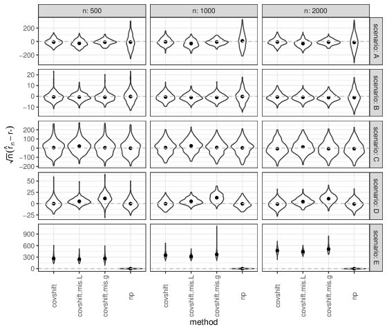
Figure S1: Sampling distribution of the scaled difference between the estimators of MSE and the true MSE in the four scenarios under covariate shift. The point stands for the empirical average in Monte Carlo simulations.

Figure S1 presents the sampling distribution of scaled difference between the four estimators of MSE and the true MSE in the five scenarios. When the dataset shift condition DS.3 holds (Scenarios A–D), np and covshift both appear close to normal and centered around the truth; in contrast, covshift.mis.L and covshift.mis.g appear more biased in Scenario D where the nuisance function estimators are substantially far from the truth, but they appear to be consistent in all scenarios. These two estimators, though generally not root-$n$ consistent and asymptotically normal, appear similar to covshift in Scenarios A–C. Thus, the asymptotic linearity of our proposed estimator might be robust against mild inconsistent estimation of one nuisance function. The variance of covshift is much smaller than that of np in both Scenarios A and B, indicating a large efficiency gain; in Scenarios C and D, the variance of these two estimators is comparable. These results are consistent with Corollary 5. When Condition DS.3 does not hold (Scenario E), our proposed estimator is substantially biased, indicating that $\hat{r}_{{\mathrm{cov}}}$ is not robust against failure of covariate shift condition DS.3.

S6 Additional results on other dataset shift conditions

In this section, we present additional results for dataset shift conditions other than sequential conditionals and its special cases (Conditions DS.0–DS.4). As in Supplement S3, we use a superscript $\dagger$ in the labels to represent results parallel to those in Section 6 in the main text.

S6.1 Posterior drift conditions

Condition DS.5^† (Posterior Drift).

Condition DS.5 holds and $X\mathchoice{\mathrel{\hbox to0.0pt{$\displaystyle\perp$\hss}\mkern 2.0mu{\displaystyle\perp}}}{\mathrel{\hbox to0.0pt{$\textstyle\perp$\hss}\mkern 2.0mu{\textstyle\perp}}}{\mathrel{\hbox to0.0pt{$\scriptstyle\perp$\hss}\mkern 2.0mu{\scriptstyle\perp}}}{\mathrel{\hbox to0.0pt{$\scriptscriptstyle\perp$\hss}\mkern 2.0mu{\scriptscriptstyle\perp}}}A$.

(Scott, 2019) further assumed $\tilde{\phi}_{*}$ (and thus $\phi_{*}$) to be strictly increasing in the original conditions. We have dropped the monotonicity requirement on $\tilde{\phi}_{*}$ because this condition does not change the geometry of the induced semiparametric model. Nevertheless, the monotonicity condition may be useful when constructing an efficient estimator of the risk $r_{*}$ if the nuisance function $\tilde{\phi}_{*}$ needs to be estimated. We have additionally assumed differentiability of $\tilde{\phi}_{*}$ (and $\phi_{*}$) to ensure sufficient smoothness of the density and the risk functional $P\mapsto R(P)=\mathbb{E}_{P}[\ell(X,Y)\mid A=0]$.

Cai and Wei (2021) used a different condition for posterior drift, namely that the supports of $P_{*,X\mid A=0}$ and $P_{*,X\mid A=1}$ are the same. This latter condition in Cai and Wei (2021) does not change the geometry of the model space and therefore we do not study it here.

Theorem 3^†.

With the notations in Theorem 3, under Condition DS.5^†, the efficient influence function for estimating $r_{*}$ is $D_{\mathrm{pd}}:o\mapsto\mathcal{E}_{*}(x)-r_{*}+F(g_{1},g_{2})(o)$.

S6.2 Location-scale shift conditions

Condition DS.6^† (Location-Scale Conditional Shift).

Condition DS.6 holds and $Y\mathchoice{\mathrel{\hbox to0.0pt{$\displaystyle\perp$\hss}\mkern 2.0mu{\displaystyle\perp}}}{\mathrel{\hbox to0.0pt{$\textstyle\perp$\hss}\mkern 2.0mu{\textstyle\perp}}}{\mathrel{\hbox to0.0pt{$\scriptstyle\perp$\hss}\mkern 2.0mu{\scriptstyle\perp}}}{\mathrel{\hbox to0.0pt{$\scriptscriptstyle\perp$\hss}\mkern 2.0mu{\scriptscriptstyle\perp}}}A$.

Zhang et al. (2013) further assumed that $W_{*}(y)$ is diagonal, but not necessarily invertible. We have relaxed the requirement that $W_{*}(y)$ is diagonal, but restricted to invertible matrices for analytic tractability.

Theorem 4^†.

Suppose that the distribution of $X\mid A=a,Y=y$ has a differentiable Lebesgue density supported on ^d for all $a\in\{0,1\}$ and $y\in\mathcal{Y}$. With the notations in Theorem 4, under Condition DS.6^†, the efficient influence function for estimating $r_{*}$ is $D_{\mathrm{lscs}}:o\mapsto\mathcal{E}_{*,Y}(y)-r_{*}+N(o)$.

S6.3 Invariant density ratio condition

Tasche (2017) introduced the following dataset shift condition for a binary label $Y\in\{0,1\}$.

Condition DS.S1 (Invariant density ratio).

The following equality between two Radon-Nikodym derivatives holds:

$$\frac{{\mathrm{d}}P_{*,X\mid Y=1,A=1}}{{\mathrm{d}}P_{*,X\mid Y=0,A=1}}=\frac{{\mathrm{d}}P_{*,X\mid Y=1,A=0}}{{\mathrm{d}}P_{*,X\mid Y=0,A=0}}.$$ (S16)

This condition is implied by label shift (DS.4), since the latter is the special case where the two Radon-Nikodym derivatives in (S16) are both constants.

However, we next argue that this condition is identical to label shift (DS.4) unless $X$ is uninformative of $Y$, and therefore do not further investigate this condition. By Bayes’ Theorem, Condition DS.S1 is equivalent to

$$\frac{P_{*}(Y=1\mid X=x,A=1)}{P_{*}(Y=0\mid X=x,A=1)}\frac{P_{*}(Y=0\mid A=1)}{P_{*}(Y=1\mid A=1)}$$

$$=\frac{P_{*}(Y=1\mid X=x,A=0)}{P_{*}(Y=0\mid X=x,A=0)}\frac{P_{*}(Y=0\mid A=0)}{P_{*}(Y=1\mid A=0)}.$$

With $\mathrm{Odds}(Y\mid X,A):=P_{*}(Y=1\mid X,A)/P_{*}(Y=0\mid X,A)$ and $\mathrm{Odds}(Y\mid A):=P_{*}(Y=1\mid A)/P_{*}(Y=0\mid A)$, this condition is further equivalent to

$$\frac{\mathrm{Odds}(Y\mid X=x,A=1)}{\mathrm{Odds}(Y\mid X=x,A=0)}=\frac{\mathrm{Odds}(Y\mid A=1)}{\mathrm{Odds}(Y\mid A=0)}.$$

In other words, a conditional odds ratio equals a marginal odds ratio; that is, the odds ratio is collapsible. As shown by Theorem 1 in Ducharme and Lepage (1986) as well as Theorem 4 and its discussion in Xie et al. (2008), odds ratios are collapsible only in rare cases, and the above equality implies that one of the following three cases holds:

1. $A\mathchoice{\mathrel{\hbox to0.0pt{$\displaystyle\perp$\hss}\mkern 2.0mu{\displaystyle\perp}}}{\mathrel{\hbox to0.0pt{$\textstyle\perp$\hss}\mkern 2.0mu{\textstyle\perp}}}{\mathrel{\hbox to0.0pt{$\scriptstyle\perp$\hss}\mkern 2.0mu{\scriptstyle\perp}}}{\mathrel{\hbox to0.0pt{$\scriptscriptstyle\perp$\hss}\mkern 2.0mu{\scriptscriptstyle\perp}}}X\mid Y$, which is identical to label shift (DS.4);

2. $Y\mathchoice{\mathrel{\hbox to0.0pt{$\displaystyle\perp$\hss}\mkern 2.0mu{\displaystyle\perp}}}{\mathrel{\hbox to0.0pt{$\textstyle\perp$\hss}\mkern 2.0mu{\textstyle\perp}}}{\mathrel{\hbox to0.0pt{$\scriptstyle\perp$\hss}\mkern 2.0mu{\scriptstyle\perp}}}{\mathrel{\hbox to0.0pt{$\scriptscriptstyle\perp$\hss}\mkern 2.0mu{\scriptscriptstyle\perp}}}X\mid A$;

3. $(A,Y)\mathchoice{\mathrel{\hbox to0.0pt{$\displaystyle\perp$\hss}\mkern 2.0mu{\displaystyle\perp}}}{\mathrel{\hbox to0.0pt{$\textstyle\perp$\hss}\mkern 2.0mu{\textstyle\perp}}}{\mathrel{\hbox to0.0pt{$\scriptstyle\perp$\hss}\mkern 2.0mu{\scriptstyle\perp}}}{\mathrel{\hbox to0.0pt{$\scriptscriptstyle\perp$\hss}\mkern 2.0mu{\scriptscriptstyle\perp}}}X$.

In the latter two cases, the covariate $X$ has no predictive power for the label $Y$. Therefore, we have shown that Condition DS.S1 is identical to label shift (DS.4) unless $X$ is uninformative of $Y$.

S7 Analysis of HIV risk prediction data in South Africa

S7.1 Analysis under each of Conditions DS.1–DS.4

We illustrate our methods by evaluating the performance of HIV prediction models using a dataset from a South African cohort study (Tanser et al., 2013). The study was a large population-based prospective cohort study in KwaZulu-Natal, South Africa. In this study, 16,667 individuals that were HIV-uninfected at baseline were followed up from 2004 to 2011.

In this analysis, we used HIV seroconversion as the outcome $Y$ and used the following covariates: number partners in the past 12 months, current marital status, wealth quintile, age and sex, community antiretroviral therapy (ART) coverage, and community HIV relevance. All covariates are binned and discrete. We set individuals from peri-urban communities with community ART coverage below 15% as the target population and those from urban and rural communities as the source population. There are 1,418 individuals from the target population and 12,385 from the source population. We used the last observed value for time-varying covariates, and missing data was treated as a separate category (Groenwold et al., 2012).

We randomly selected half of the source population data as the held-out dataset to train an HIV risk prediction model $f$. We then used the other half of the source population data and randomly selected 50 individuals from the target population to estimate the inaccuracy of $f$ in the target population (recall Example 1). In other words, we had a large source population data and a small target population data. We applied the nonparametric estimator $\hat{r}_{{\mathrm{np}}}$ and our proposed efficient estimator under each of the four most common dataset shift conditions DS.1–DS.4 connecting these two populations. We used the rest of the target population data as a validation dataset to obtain a good estimate of the risk and evaluate the performance of risk estimators.

In all regressions, to obtain potentially improved nuisance regression function estimators and make sufficient conditions for our estimators’ efficiency more plausible, we further added single hidden layer feedforward neural networks with various numbers of hidden nodes into the Super Learner library that we used for the simulations. With an appropriate number of hidden nodes, such neural networks have been shown to achieve an ${\mathrm{o}}_{p}(n^{-1/4})$ convergence rate under mild smoothness conditions (Chen and White, 1999).

Since we do not expect the individuals from the two populations to be similar random draws from a common population, concept shift assumption (either DS.1 or DS.2) might fail and their corresponding efficient estimators might be biased. Since covariates are likely to affect the outcome causally and the other causal direction is implausible due to time ordering, Assumption DS.4 might also fail. The covariates may have reasonable predictive power, and thus Assumption DS.3 may approximately hold. In the analysis, we also tested whether the efficient estimator under each dataset shift condition is consistent for the risk of interest using the specification test implied by Corollary 1.

Table S1: Risk estimates under at most one dataset shift condition on the source population. The risk estimate from the validation dataset is 0.24 (95% confidence interval: 0.22–0.26). All confidence intervals (CIs) are Wald intervals.

Dataset Shift Condition	Estimate	S.E.	95% CI	P-value
None	0.24	0.060	(0.12, 0.36)	—
Concept shift in the features DS.1	0.26	0.057	(0.15, 0.38)	0.29
Concept shift in the labels DS.2	0.10	0.010	(0.08, 0.12)	0.02
Full-data covariate shift DS.3	0.19	0.026	(0.14, 0.25)	0.41
Full-data label shift DS.4	0.23	0.059	(0.11, 0.34)	0.42

The risk estimates and the p-values for testing the four dataset shift conditions are presented in Table S1. As expected, our proposed estimator under concept shift in the labels (DS.2) is biased and this dataset shift condition can be rejected at level 0.05, indicating evidence that concept shift in the labels does not hold. Concept shift in the features (DS.1) is not rejected, and our proposed estimator under this condition leads to a similar conclusion to the nonparametric estimator with a confidence interval that is around 5% shorter. Label shift assumption (DS.4) is not rejected either, and our proposed estimator under this condition leads to an almost identical conclusion compared to the nonparametric estimator. Covariate shift (DS.3) is also not rejected, and our proposed efficient estimator has a much smaller standard error, leading to a confidence interval that is more than 50% shorter. We emphasize that our test may be underpowered, so failure to reject these dataset shift conditions should not be interpreted as strong evidence that these conditions may be plausible. Since covariate shift is the most plausible assumption among the four a priori—although, in this particular case, all point estimates appear consistent except for concept shift in the labels, for which we find evidence of bias—we conclude that using our proposed efficient estimator under a conceivable dataset shift condition may lead to substantial efficiency gains and thus more informative estimates of risk, namely with substantially smaller variance.

S7.2 Semi-synthetic data analysis

For each of Conditions DS.1–DS.4, we also conducted a semi-synthetic data analysis. Using the original data $D$ analyzed in Section S7, we generated a semi-synthetic dataset satisfying the dataset shift condition under consideration. We then ran a similar analysis as in Section S7. We next describe the semi-synthetic data-generating procedures in more detail and report the analysis results. From our analyses, we conclude that, under a plausible dataset shift condition, our proposed efficient risk estimator that fully exploits the dataset shift condition may lead to substantial efficiency gains and shorter CIs.

S7.2.1 Concept shift in the features (DS.1)

To generate a semi-synthetic data satisfying Condition DS.1, we first randomly generated the synthetic population indicator $A$ following the empirical distribution observed in the original data $D$ and then set the outcome $Y$ to be missing for individuals from the synthetic source population ($A=1$). We left the covariate $X$ in both synthetic populations and the outcome $Y$ in the synthetic target population unchanged. In the analysis, we used 50 individuals from the synthetic target population to train a prediction model $f$. We then used all individuals from the synthetic source population and 50 individuals from the synthetic target population to estimate the risk of $f$. We used the rest of the individuals from the synthetic target population as the validation dataset to evaluate the performance of risk estimators.

The risk estimate from the validation dataset is 0.10 with a 95% confidence interval (CI) of 0.09–0.12. The estimate under no dataset shift condition is 0.06 (S.E.: 0.034, 95% CI: 0–0.13); the estimate from our proposed estimator is 0.06 (S.E.: 0.033, 95% CI: 0–0.12). Here, the CIs are truncated to fall in the unit interval $[0,1]$. The test of Condition DS.1 yields a p-value $>0.99$, correctly indicating that Condition DS.1 may be plausible in this semi-synthetic dataset. The CI based on our proposed estimator is almost identical to that based on the nonparametric estimator. The small efficiency gain might be attributed to the limited sample size to learn the conditional mean risk function $\mathcal{E}_{*}$, which is a function of the moderately high-dimensional covariate $X$ and thus difficult to estimate accurately; additional information about the distribution of $X$ cannot improve estimation of $\mathcal{E}_{*}$.

S7.2.2 Concept shift in the labels (DS.2)

Our data-generating procedure and analysis are similar to those in Section S7.2.1. The only difference is that we set covariate $X$, rather than outcome $Y$, to be missing in the synthetic source population.

The risk estimate from the validation dataset is 0.10 (95% CI: 0.09–0.12). The nonparametric estimate is 0.12 (S.E.: 0.046, 95% CI: 0.03–0.21), while the estimate from our proposed estimator is 0.14 (S.E.: 0.035, 95% CI: 0.07–0.21). The p-value of from the test of Condition DS.2 is 0.53. The CI based on our proposed estimator is more than 20% shorter than that based on the nonparametric estimator.

S7.2.3 Full-data covariate shift (DS.3)

To generate a semi-synthetic dataset satisfying Condition DS.3, we first randomly split the original dataset $D$ into two halves $D_{1}$ and $D_{2}$. We used $D_{1}$ to obtain estimates $\hat{g}$ and $\hat{\mathcal{L}}$ of nuisance functions $g_{*}:x\mapsto P_{*}(A=0\mid X=x)$ and $\mathcal{L}_{*}:x\mapsto\mathbb{E}_{P_{*}}[Y\mid X=x]=P_{*}(Y=1\mid X=x)$, respectively. With the observed covariates $X$ in $D_{2}$, we generated synthetic population indicator $A$ and synthetic outcome $Y$ independently given $X$ based on $\hat{g}$ and $\hat{\mathcal{L}}$, respectively. We used this semi-synthetic dataset in the subsequent analysis. We used half of the individuals from the synthetic source population to train a prediction model $f$. We then used the other half of the individuals from the synthetic source population and 50 individuals from the synthetic target population to estimate the risk of $f$. We used the rest of the individuals from the synthetic target population as the validation dataset.

In the validation dataset, the risk is estimated to be 0.22 (95% CI: 0.19–0.26). The nonparametric risk estimator yields a point estimate of 0.20 with S.E. 0.057 and 95% CI 0.09–0.31; our proposed estimator yields a point estimate of 0.23 with S.E. 0.030 and 95% CI 0.17–0.29. Condition DS.3 is not rejected (p-value=0.51). The CI based on our proposed estimator is about 50% shorter than that based on the nonparametric estimator.

S7.2.4 Full-data label shift (DS.4)

The data-generating procedure is similar to that in Section S7.2.3. A major difference is that, when generating synthetic covariate $X$ and synthetic population indicator $A$ in $D_{2}$, we sample $X$ and $A$ independently given $Y$ from the empirical distribution of $X\mid Y$ and $A\mid Y$ observed in $D_{1}$. We could use the empirical distribution because $Y$ is binary. Super Learner uses cross-validation to select the weight to ensemble learners in the library, and cross-validation can be problematic with ties in the data (Bickel et al., 1997). To alleviate this issue, for each covariate of each individual in the semi-synthetic data, we independently replaced the observed value with a uniform draw from the range of this covariate with 10% probability. Such random corruption for discrete variables has been extensively studied (e.g., Ma et al., 2018; Angluin and Laird, 1988; Aslam and Decatur, 1996, etc.).

In the validation dataset, the risk is estimated to be 0.27 (95% CI: 0.24–0.31). The estimates from the nonparametric estimator and our proposed estimator are 0.20 (S.E.: 0.057, 95% CI: 0.09–0.31) and 0.21 (S.E.: 0.056, 95% CI: 0.11–0.32), respectively. Condition DS.4 is not rejected (p-value=0.07). The length of the CI based on our proposed estimator is almost identical to than that based on the nonparametric estimator. The similar performance of these two estimators in this analysis may be explained by the fact that, under label shift (DS.4), a main contribution from the source population is additional data to estimate the conditional mean risk function $\mathcal{L}_{*,Y}$. Since $Y$ is binary, $\mathcal{L}_{*,Y}$ can be estimated fairly accurately with the target population data alone, and the improvement in the risk estimator due to the improved estimation of $\mathcal{L}_{*,Y}$ is limited.

S8 Prediction set construction based on risk estimation

Following Example 2, in this supplement, we briefly review a few coverage guarantees for prediction sets and describe how our risk estimation methods can be helpful in constructing prediction sets. We consider using a dataset with the structure described in Section 2 and sample size $n$ to construct a prediction set function $\hat{C}:\mathcal{X}\to\mathscr{B}$, where $\mathscr{B}\subseteq 2^{\mathcal{Y}}$ is a Borel sigma algebra on $\mathcal{Y}$. We focus on coverage guarantees in the target population. We slightly abuse terminology and also call $\hat{C}$ a prediction set.

Most of the popular coverage guarantees fall into two categories: (i) marginal validity, and (ii) training-set conditional validity, also termed Probably Approximately Correct (PAC). A discussion of the differences between these two categories can be found in the Supplementary Material of Qiu et al. (2022). We describe these two categories in the following subsections. More details on this topic can be found in, for example, Angelopoulos et al. (2021); Balasubramanian et al. (2014); Barber et al. (2022); Bian and Barber (2022); Chernozhukov et al. (2018b); Lei et al. (2015); Lei and Candès (2021); Park et al. (2020, 2022); Qiu et al. (2022); Tibshirani et al. (2019); Shafer and Vovk (2008); Vovk et al. (1999, 2005); Vovk (2013); Yang et al. (2022).

S8.1 Marginal validity

A prediction set $\hat{C}$ is said to achieve marginal validity with coverage error at most $\alpha\in(0,1)$ if $P_{*}(Y\notin\hat{C}(X)\mid A=0)\leq\alpha$, where the triple $(X,Y,A)$ is a new draw from $P_{*}$ independent of the training data. This finite-sample guarantee can be achieved by applying conformal prediction methods to the target population data while ignoring the source population data (see, e.g., Shafer and Vovk, 2008; Vovk et al., 1999, 2005; Vovk, 2013, etc.).

However, if the source population data is relevant under a dataset shift condition (e.g., one of Conditions DS.1–DS.4), it may be possible to prediction sets of smaller sizes with an asymptotic marginal coverage guarantee, namely $P_{*}(Y\notin\hat{C}(X)\mid A=0)\leq\alpha+{\mathrm{o}}(1)$. Such guarantees have been adopted when dataset shift is present (see, e.g., Lei and Candès, 2021; Tibshirani et al., 2019; Yang et al., 2022).

Suppose that a predictor $f$ trained on a held-out dataset and a scoring function $s:\mathcal{X}\times\mathcal{Y}\to\real$ are given. Without loss of generality, we assume that a higher score corresponds to more conformity. For example, when the outcome $Y$ is continuous, a common scoring function is $s(x,y)=-|y-f(x)|$; when the label $Y$ is discrete and $f(x)$ is a vector of estimated probabilities $P_{*}(Y=y\mid X=x)$, a common scoring function is $s(x,y)=f_{y}(x)$, the $y$-th entry of $f(x)$. For simplicity in our illustration, we assume that the distribution of $s(X,Y)\mid A=0$ is continuous.

Consider prediction sets of the form $C_{\tau}:x\mapsto\{y\in\mathcal{Y}:s(x,y)\geq\tau\}$, where $\tau\in\real\cup\{\pm\infty\}$ is a threshold. Following the approach from Yang et al. (2022), given an estimator $\hat{r}_{\tau}$ of the coverage error $r_{*,\tau}:=\mathbb{E}_{P_{*}}[{\mathbbm{1}}(Y\notin C_{\tau}(X))\mid A=0]$ of $C_{\tau}$ that is consistent uniformly over $\tau$, we may find an appropriate threshold $\hat{\tau}$ by solving the estimating equation $\hat{r}_{\tau}=\alpha$ for $\tau$. If $\hat{r}_{\tau}$ is efficient, we expect that, with a high probability, $\hat{r}_{\tau}$ is close to $r_{*,\tau}$ and thus the selected threshold $\hat{\tau}$ is close to the true optimal threshold $\tau_{*}$, the $\alpha$-th quantile of $s(X,Y)\mid A=0$. In other words, the sampling distribution of $\hat{\tau}$ is expected to be more concentrated around $\tau_{*}$ compared to the threshold selected based on an inefficient estimator of $r_{*,\tau}$.

S8.2 Training-set conditional validity

A prediction set $\hat{C}$ is said to achieve training-set conditional validity, or to be $(\alpha,\delta)$-PAC, if $P_{*}(P_{*}(Y\notin\hat{C}(X)\mid A=0,\text{training data})\leq\alpha)\geq 1-\delta$, where the triple $(X,Y,A)$ is independent of the training data. This guarantee implies marginal validity with coverage error at most $\alpha+\delta$ by a union bound (see, e.g., Lemma S2 in Qiu et al., 2022). Similarly to marginal validity, this finite-sample guarantee can be achieved by applying split (or inductive) conformal prediction to the target population data while ignoring the source population data (see, e.g., Park et al., 2020; Vovk, 2013).

Using the source population data and our proposed efficient risk estimators, it is possible to construct prediction sets of smaller sizes with asymptotic training-set conditional validity. Qiu et al. (2022) identified two types of asymptotic training-set conditional validity: (i) Asymptotically Probably Approximately Correct (APAC), where $P_{*}(P_{*}(Y\notin\hat{C}(X)\mid A=0,\text{training data})\leq\alpha)\geq 1-\delta-{\mathrm{o}}(1)$, and (ii) Probably Asymptotically Approximately Correct (PAAC), where $P_{*}(P_{*}(Y\notin\hat{C}(X)\mid A=0,\text{training data})\leq\alpha+{\mathrm{o}}_{p}(1))\geq 1-\delta$. See Qiu et al. (2022) for a thorough discussion of the similarities and differences between these guarantees. In many cases, PAAC is similar to asymptotic marginal validity (see, e.g., Bian and Barber, 2022; Yang et al., 2022), and thus the approach we described in Section S8.1 can be adopted.

In contrast, the APAC guarantee requires techniques more similar to those used for obtaining PAC guarantees. We consider a setup similar to Section S8.1 and follow the approaches of Angelopoulos et al. (2021); Qiu et al. (2022) based on multiple testing. Let $\mathcal{T}\subseteq\real\cup\{\pm\infty\}$ be a given finite set of candidate thresholds, and $U_{\tau}$ be an upper confidence bound for $r_{*,\tau}=\mathbb{E}_{P_{*}}[{\mathbbm{1}}(Y\notin C_{\tau}(X))\mid A=0]$, whose coverage probability converges to $1-\delta$ uniformly over $\tau\in\mathcal{T}$. Then a threshold $\hat{\tau}$ can be selected as $\max\{\tau\in\mathcal{T}:U_{\tau^{\prime}}<\alpha\text{ for all }\tau^{\prime}\in\mathcal{T}\text{ such that }\tau^{\prime}\leq\tau\}$, and $C_{\hat{\tau}}$ would be APAC. Such an upper confidence bound can be constructed based on asymptotic linear estimators $\hat{r}_{\tau}$ of $r_{*}=\mathbb{E}_{P_{*}}[{\mathbbm{1}}(Y\notin C_{\tau}(X))\mid A=0]$ via, for example, normal approximation or bootstrap. Efficient estimators would lead to small confidence upper bounds and thus a selected threshold $\hat{\tau}$ close to the true optimal threshold $\tau_{*}$. In other words, the sampling distribution of $\hat{\tau}$ is expected to be less conservative and lead to smaller prediction sets, compared to the threshold selected based on an inefficient estimator of $r_{*,\tau}$.

S9 Proofs

S9.1 Review of basic results in semiparametric efficiency theory

The following lemma contains basic results in semiparametric efficiency theory and can be easily proved by the law of total expectation.

Lemma S1.

Each collection of subspaces of $L^{2}(P_{*})$ in the following list is mutually orthogonal:

• $L^{2}(P_{*,X})$, ${\mathcal{T}}_{A\mid X}$, ${\mathcal{T}}_{Y\mid X,A}$;

• $L^{2}(P_{*,A})$, ${\mathcal{T}}_{X\mid A}$, ${\mathcal{T}}_{Y\mid X,A}$;

• $L^{2}(P_{*,X,A})$, ${\mathcal{T}}_{Y\mid X,A}$;

• $L^{2}(P_{*,A})$, ${\mathcal{T}}_{Z_{k}\mid\bar{Z}_{k-1},A}$ ($k\in[K]$).

Consequently, $L^{2}_{0}(P_{*})={\mathcal{T}}_{A}\oplus\{\oplus_{k=1}^{K}{\mathcal{T}}_{\bar{Z}_{k}\mid\bar{Z}_{k-1},A}\}$; for any function $f\in L^{2}_{0}(P_{*})$, the projection of $f$ onto ${\mathcal{T}}_{\sharp}$ is $s\mapsto\mathbb{E}_{P_{*}}[f(O)\mid\sharp=s]$, and the projection of $f\in L^{2}_{0}(P_{*})$ onto ${\mathcal{T}}_{\sharp\mid\natural}$ is $(s,t)\mapsto\mathbb{E}_{P_{*}}[f(O)\mid\sharp=s,\natural=t]-\mathbb{E}_{P_{*}}[f(O)\mid\natural=t]$.

When we derive the efficient influence function for each dataset shift condition, we first characterize the tangent space at $P_{*}$, which is a subspace of the nonparametric tangent space $L^{2}_{0}(P_{*})$. We also characterize the orthogonal complement of the tangent space. The efficient influence function is then the projection of the nonparametric influence function $D_{\mathrm{np}}(P_{*},r_{*})$ onto the tangent space. We also ignore the difference between “almost everywhere” and “everywhere” for convenience; the exceptional probability-zero set can always be excluded from our analysis.

S9.2 No dataset shift condition: nonparametric model

The following lemma states the asymptotic efficiency of the nonparametric estimator $\hat{r}_{{\mathrm{np}}}$ under a nonparametric model.

Lemma S2.

Under a nonparametric model at $P_{*}$, the efficient influence function for estimating $r_{*}$ is $D_{\mathrm{np}}(\rho_{*},r_{*})$ from (3). The sequence of estimators $\hat{r}_{{\mathrm{np}}}$ is RAL with the influence function $D_{\mathrm{np}}(\rho_{*},r_{*})$, and thus is nonparametrically efficient. Consequently, $\sqrt{n}(\hat{r}_{{\mathrm{np}}}-r_{*})\overset{d}{\to}\mathrm{N}(0,\sigma_{*,{\mathrm{np}}}^{2})$ with $\sigma_{*,{\mathrm{np}}}^{2}:=\mathbb{E}_{P_{*}}[D_{\mathrm{np}}(\rho_{*},r_{*})$$(O)^{2}]$.

Proof.

We first prove that $D_{\mathrm{np}}(P_{*},r_{*})$ is the efficient influence function. Let $H$ be an arbitrary bounded function in $L^{2}_{0}(P_{*})$. The $L^{2}(P_{*})$-closure of the collection of such functions is $L^{2}_{0}(P_{*})$. Consider the projections of $H$ onto ${\mathcal{T}}_{A}$ and ${\mathcal{T}}_{Z\mid A}$, respectively:

$$H_{A}:a\mapsto\mathbb{E}_{P_{*}}[H(O)\mid A=a],\quad H_{Z\mid A}:(z\mid a)\mapsto H(O)-H_{A}(a).$$

Define a regular parametric submodel indexed by $\varepsilon$ via

$$\left\{P^{\varepsilon}:\frac{{\mathrm{d}}P^{\varepsilon}}{{\mathrm{d}}P_{*}}(o)=(1+\varepsilon H_{A}(a))(1+\varepsilon H_{Z\mid A}(z\mid a))\right\}$$

for $\varepsilon$ in a small neighborhood of zero such that $P^{\varepsilon}$ has non-negative density with respect to $P_{*}$. Clearly, $P^{\varepsilon}=P_{*}$ at $\varepsilon=0$. Further, by Bolthausen et al. (Lemma 1.8 in Part III 2002) and direct calculation, one can verify that and this submodel is a differentiable path at $\varepsilon=0$ with score function being $H$ (see, e.g., Definition 1.6 in Part III of Bolthausen et al., 2002).

Recall that $R(P)$ denotes the risk in the target population associated with data-generating distribution $P$, namely $\mathbb{E}_{P}[\ell(Z)\mid A=0]$. To show that $R(P)$ is differentiable at $P_{*}$ relative to the tangent set $L^{2}_{0}(P_{*})$, with efficient influence function $D_{\mathrm{np}}(\rho_{*},r_{*})$, it suffices to show that

$$\left.\frac{{\mathrm{d}}R(P^{\varepsilon})}{{\mathrm{d}}\varepsilon}\right|_{\varepsilon=0}=P_{*}HD_{\mathrm{np}}(\rho_{*},r_{*}),$$ (S17)

since, for nonparametric models, the tangent space is $L^{2}_{0}(P_{*})$ and the influence function is unique (see, e.g., Example 1.12 in Part III of Bolthausen et al., 2002).

We next derive (S17). By definition,

$$R(P)=\int\ell(z)P_{Z\mid A}({\mathrm{d}}z\mid 0).$$

Thus, since integration and differentiation can be interchanged due to boundedness,

$$\left.\frac{{\mathrm{d}}R(P^{\varepsilon})}{{\mathrm{d}}\varepsilon}\right|_{\varepsilon=0}=\int\ell(z)H_{Z\mid A}(z\mid 0)P_{*,Z\mid A}({\mathrm{d}}z\mid 0).$$

Since $H_{Z\mid A}\in{\mathcal{T}}_{Z\mid A}$ has mean zero conditional on $A$, we may center $\ell(z)$ and show that the quantity on the right-hand side above equals

$$\int(\ell(z)-r_{*})H_{Z\mid A}(z\mid 0)P_{*,Z\mid A}({\mathrm{d}}z\mid 0).$$

We can further use inverse-probability weighting to take into account the randomness in $A$ to show that the above quantity equals

$$\iint\frac{{\mathbbm{1}}(a=0)}{\rho_{*}}(\ell(z)-r_{*})H_{Z\mid A}(z\mid a)P_{*,Z\mid A}({\mathrm{d}}z\mid a)P_{*,A}({\mathrm{d}}a).$$

Since $o\mapsto\ell(z)-r_{*}$ is orthogonal to $o\mapsto\frac{{\mathbbm{1}}(a=0)}{\rho_{*}}H_{A}(a)$, the above quantity further equals

$$\iint\frac{{\mathbbm{1}}(a=0)}{\rho_{*}}(\ell(z)-r_{*})\{H_{Z\mid A}(z\mid a)+H_{A}(a)\}P_{*,Z\mid A}({\mathrm{d}}z\mid a)P_{*,A}({\mathrm{d}}a)$$

$$=\int\frac{{\mathbbm{1}}(a=0)}{\rho_{*}}(\ell(z)-r_{*})H(o)P_{*}({\mathrm{d}}o)=P_{*}HD_{\mathrm{np}}(\rho_{*},r_{*}).$$

We have shown that $D_{\mathrm{np}}(\rho_{*},r_{*})$ is the efficient influence function.

We next show that the influence function of $\hat{r}_{{\mathrm{np}}}$ is $D_{\mathrm{np}}(\rho_{*},r_{*})$. By the central limit theorem,

$$\frac{1}{n}\sum_{i=1}^{n}{\mathbbm{1}}(A_{i}=0)\ell(Z_{i}) =\rho_{*}r_{*}+\frac{1}{n}\sum_{i=1}^{n}\{{\mathbbm{1}}(A_{i}=0)\ell(Z_{i})-\rho_{*}r_{*}\}=\rho_{*}r_{*}+{\mathrm{O}}_{p}\left(\frac{1}{n^{1/2}}\right)$$

and $\frac{1}{n}\sum_{i=1}^{n}{\mathbbm{1}}(A_{i}=0)=\rho_{*}+\frac{1}{n}\sum_{i=1}^{n}\{{\mathbbm{1}}(A_{i}=0)-\rho_{*}\}=\rho_{*}+{\mathrm{O}}_{p}(n^{-1/2})$. Hence, by a Taylor expansion of $x\mapsto 1/x$ around $\rho_{*}>0$, we have that

$$\hat{r}_{{\mathrm{np}}}=\frac{\frac{1}{n}\sum_{i=1}^{n}{\mathbbm{1}}(A_{i}=0)\ell(Z_{i})}{\frac{1}{n}\sum_{i=1}^{n}{\mathbbm{1}}(A_{i}=0)}=\frac{\rho_{*}r_{*}+\frac{1}{n}\sum_{i=1}^{n}\{{\mathbbm{1}}(A_{i}=0)\ell(Z_{i})-\rho_{*}r_{*}\}}{\rho_{*}+\frac{1}{n}\sum_{i=1}^{n}\{{\mathbbm{1}}(A_{i}=0)-\rho_{*}\}}$$

$$=\left[\rho_{*}r_{*}+\frac{1}{n}\sum_{i=1}^{n}\{{\mathbbm{1}}(A_{i}=0)\ell(Z_{i})-\rho_{*}r_{*}\}\right]\times\left[\frac{1}{\rho_{*}}-\frac{1}{\rho_{*}^{2}}\frac{1}{n}\sum_{i=1}^{n}\{{\mathbbm{1}}(A_{i}=0)-\rho_{*}\}+{\mathrm{o}}_{p}(n^{-1/2})\right]$$

$$=r_{*}+\frac{1}{n}\sum_{i=1}^{n}D_{\mathrm{np}}(\rho_{*},r_{*})(O_{i})+{\mathrm{o}}_{p}(n^{-1/2}).$$

We have thus shown that $\hat{r}_{{\mathrm{np}}}$ is asymptotically linear with influence function $D_{\mathrm{np}}(\rho_{*},r_{*})$. Its regularity and asymptotic efficiency follow from Lemma 2.9 in Part III of Bolthausen et al. (2002). ∎

S9.3 General sequential conditionals

Proof of the efficiency bound under Condition DS.0.

This result is implied by Theorem 2 and Corollary 1 from Li and Luedtke (2023). Specifically, our Condition DS.0 reduces to Conditions 1 and 2 from Li and Luedtke (2023) with the target population distribution—$\underline{Q}^{0}$ in their notation—being the distribution of $Z\mid A=0$ under $P_{*}$. Moreover, our $A$ is their $S$, and our $\mathcal{S}_{k}^{\prime}$ is their $\mathcal{S}_{k}$.

By Bayes’ Theorem, the Radon-Nikodym derivative of the distribution of $\bar{Z}_{k-1}\mid A=0$ relative to $\bar{Z}_{k-1}\mid A\in\mathcal{S}^{\prime}_{k}$—$\lambda_{k-1}$ in their notation—is shown in (S2), and is uniformly bounded away from zero and infinity in the support $\mathcal{Z}_{k-1}$ of $\bar{Z}_{k-1}\mid A=0$—which is $\mathcal{Z}^{\dagger}_{j-1}$ in their notation. Hence, Condition 3 from Li and Luedtke (2023) is also satisfied.

Moreover, when the observed data is only from the target population, since we impose no restriction on the distribution of $Z$ in the target population, the corresponding tangent space—$\mathcal{T}(Q_{0},\mathcal{Q})$ in their notation—is $L^{2}(P_{*,Z\mid A=0})$; the influence function of $r_{*}$ is unique and equals $z\mapsto\ell(z)-r_{*}$. Thus, $r_{j}(\bar{z}_{j})$ in Corollary 1 from Li and Luedtke (2023) equals the product of the Radon-Nikodym derivative in (S2) and $\ell^{j}_{*}(\bar{z}_{j})-\ell^{j-1}_{*}(\bar{z}_{k-1})$, which is zero for $\bar{z}_{j}$ outside the support $\mathcal{Z}_{k-1}$ of $\bar{Z}_{k-1}\mid A=0$. We plug the above results into Corollary 1 from Li and Luedtke (2023) to obtain the claimed efficiency bound under Condition DS.0. ∎

Corollary S1 can be shown similarly.

We next present a lemma that will be useful in the proof of Theorem S1.

Lemma S3.

For every $k\in[2:K]$ and $v\in[V]$, with $B_{k}$ from (S7),

$$\left(\sum_{a\in\mathcal{S}^{\prime}_{1}}\hat{\pi}^{a}_{v}\right)\mathbb{E}_{P_{*}}\left[\frac{{\mathbbm{1}}(A\in\mathcal{S}^{\prime}_{k})}{\sum_{a\in\mathcal{S}^{\prime}_{k}}\hat{\pi}^{a}_{v}}\hat{\lambda}^{k-1}_{v}(\bar{Z}_{k-1})[\hat{\ell}^{k}_{v}(\bar{Z}_{k})-\hat{\ell}^{k-1}_{v}(\bar{Z}_{k-1})]\right]$$

$$=B_{k}+\left(\sum_{a\in\mathcal{S}^{\prime}_{1}}\pi^{a}_{*}\right)\mathbb{E}_{Q}\left[\mathbb{E}_{P_{*}}\left[\hat{\ell}^{k}_{v}(\bar{Z}_{k})\mid\bar{Z}_{k-1},A\in\mathcal{S}^{\prime}_{k}\right]-\hat{\ell}^{k-1}_{v}(\bar{Z}_{k-1})\right].$$ (S18)

Additionally, under Condition DS.S0, we have the following identity for the second term on the right-hand side of (S18):

$$\mathbb{E}_{Q}\left[\mathbb{E}_{P_{*}}\left[\hat{\ell}^{k}_{v}(\bar{Z}_{k})\mid\bar{Z}_{k-1},A\in\mathcal{S}^{\prime}_{k}\right]-\hat{\ell}^{k-1}_{v}(\bar{Z}_{k-1})\right]=\mathbb{E}_{Q}[\hat{\ell}^{k}_{v}(\bar{Z}_{k})-\hat{\ell}^{k-1}_{v}(\bar{Z}_{k-1})].$$

Proof.

Equation S18 follows by adding and subtracting $\lambda^{k-1}_{*}$ from $\hat{\lambda}^{k-1}_{v}$, by the definition of $\lambda^{k-1}_{*}$ as the Radon-Nikodym derivative of the distribution of $\bar{Z}_{k-1}$ under $Q$ relative to that of $\bar{Z}_{k-1}\mid A\in\mathcal{S}^{\prime}_{k}$ under $P_{*}$, by $P_{*}(A\in\mathcal{S}^{\prime}_{k})=\sum_{a\in\mathcal{S}^{\prime}_{k}}\pi^{a}_{*}$, and by using the law of iterated expectation. Under Condition DS.S0, for $Q$-almost every $\bar{z}_{k-1}\in\widetilde{\mathcal{Z}}_{k-1}$,

$$\mathbb{E}_{P_{*}}\left[\hat{\ell}^{k}_{v}(\bar{Z}_{k})\mid\bar{Z}_{k-1}=\bar{z}_{k-1},A\in\mathcal{S}^{\prime}_{k}\right]=\mathbb{E}_{Q}\left[\hat{\ell}^{k}_{v}(\bar{Z}_{k})\mid\bar{Z}_{k-1}=\bar{z}_{k-1}\right]$$

and the second claim follows. ∎

Proof of Theorem S1.

We study the asymptotic behavior of the estimator $\hat{r}_{v}$ for each fold $v$ via methods for analyzing Z-estimators (see, e.g., Section 3.3 in van der Vaart and Wellner, 1996), and the asymptotic behavior of the cross-fit estimator $\hat{r}$ follows immediately. By the definitions of the nuisance functions $\bm{\ell}_{*}$ from (S1), the Radon-Nikodym derivatives $\bm{\lambda}_{*}=(\lambda^{k}_{*})_{k=1}^{K-1}$, the marginal probabilities $\bm{\pi}_{*}:=(\pi_{*}^{a})_{a\in\mathcal{A}}$ of the source populations, and $D_{\mathrm{GSC}}$ from (S4), we have that

$$P_{*}\left(\sum_{a\in\mathcal{S}^{\prime}_{1}}\pi^{a}_{*}\right)D_{\mathrm{GSC}}(\bm{\ell}_{*},\bm{\lambda}_{*},\bm{\pi}_{*},r_{*})=0.$$ (S19)

By the definitions of $\widetilde{\mathcal{T}}$ from (S3), $\hat{r}_{v}$ from (S5), and $D_{\mathrm{GSC}}$ from (S4), noting that

$$\sum_{i\in I_{v}}\frac{{\mathbbm{1}}(A_{i}\in\mathcal{S}^{\prime}_{1})}{\sum_{a\in\mathcal{S}^{\prime}_{1}}\hat{\pi}_{v}^{a}}=\sum_{b\in\mathcal{S}^{\prime}_{1}}\frac{\sum_{i\in I_{v}}{\mathbbm{1}}(A_{i}=b)}{\sum_{a\in\mathcal{S}^{\prime}_{1}}\hat{\pi}_{v}^{a}}=|I_{v}|,$$

we find that

$$P^{n,v}\left(\sum_{a\in\mathcal{S}^{\prime}_{1}}\hat{\pi}^{a}_{v}\right)D_{\mathrm{GSC}}(\widehat{\bm{\ell}}_{v},\widehat{\bm{\lambda}}_{v},\widehat{\bm{\pi}}_{v},\hat{r}_{v})=0.$$

Then we have the following equation:

$$0 =(P^{n,v}-P_{*})\left\{\left(\sum_{a\in\mathcal{S}^{\prime}_{1}}\hat{\pi}^{a}_{v}\right)D_{\mathrm{GSC}}(\widehat{\bm{\ell}}_{v},\widehat{\bm{\lambda}}_{v},\widehat{\bm{\pi}}_{v},\hat{r}_{v})-\left(\sum_{a\in\mathcal{S}^{\prime}_{1}}\pi^{a}_{*}\right)D_{\mathrm{GSC}}(\bm{\ell}_{*},\bm{\lambda}_{*},\bm{\pi}_{*},r_{*})\right\}$$

$$\quad+P_{*}\left\{\left(\sum_{a\in\mathcal{S}^{\prime}_{1}}\hat{\pi}^{a}_{v}\right)D_{\mathrm{GSC}}(\widehat{\bm{\ell}}_{v},\widehat{\bm{\lambda}}_{v},\widehat{\bm{\pi}}_{v},\hat{r}_{v})-\left(\sum_{a\in\mathcal{S}^{\prime}_{1}}\pi^{a}_{*}\right)D_{\mathrm{GSC}}(\bm{\ell}_{*},\bm{\lambda}_{*},\bm{\pi}_{*},r_{*})\right\}$$

$$\quad+(P^{n,v}-P_{*})\left(\sum_{a\in\mathcal{S}^{\prime}_{1}}\pi^{a}_{*}\right)D_{\mathrm{GSC}}(\bm{\ell}_{*},\bm{\lambda}_{*},\bm{\pi}_{*},r_{*}).$$ (S20)

We refer to the three terms on the right-hand side of (S20) as Terms 1–3, respectively. We next study these three terms separately.

Term 1: By the definition of $D_{\mathrm{GSC}}$ from (S4), this term equals

$$(P^{n,v}-P_{*})\left\{\left(\sum_{a\in\mathcal{S}^{\prime}_{1}}\hat{\pi}^{a}_{v}\right)\widetilde{\mathcal{T}}(\widehat{\bm{\ell}}_{v},\widehat{\bm{\lambda}}_{v},\widehat{\bm{\pi}}_{v})-\left(\sum_{a\in\mathcal{S}^{\prime}_{1}}\pi^{a}_{*}\right)\widetilde{\mathcal{T}}(\bm{\ell}_{*},\bm{\lambda}_{*},\bm{\pi}_{*})-{\mathbbm{1}}_{\mathcal{S}^{\prime}_{1}}\left(\hat{r}_{v}-r_{*}\right)\right\}.$$

We first condition on data out of fold $v$. By the definition of $\widetilde{\mathcal{T}}$ from (S3), as well as the facts that (i) $\hat{\pi}^{a}_{v}$ is root-$n$ consistent for $\pi^{a}_{*}$, $a\in\mathcal{A}$ in $P^{n,v}$-probability, and (ii) we condition on $\widehat{\bm{\ell}}_{v},\widehat{\bm{\theta}}_{v}$, by Lemmas 9.6 and 9.9 in Kosorok (2008), we have that, with $P^{n,v}$-probability tending to one as $n\to\infty$, the random function $o\mapsto\left(\sum_{a\in\mathcal{S}^{\prime}_{1}}\hat{\pi}^{a}_{v}\right)\widetilde{\mathcal{T}}(\widehat{\bm{\ell}}_{v},\widehat{\bm{\lambda}}_{v},\widehat{\bm{\pi}}_{v})(o)-\left(\sum_{a\in\mathcal{S}^{\prime}_{1}}\pi^{a}_{*}\right)\widetilde{\mathcal{T}}(\bm{\ell}_{*},\bm{\lambda}_{*},\bm{\pi}_{*})(o)$, whose randomness comes from $\widehat{\bm{\pi}}_{v}$, falls into a fixed VC-subgraph, and thus $P_{*}$-Donsker, class. We also have that, since $\hat{r}_{v}$ from (S5) is a constant as a function $X$ over which the expectation with respect to $P^{*}$ is evaluated, $(P^{n,v}-P_{*}){\mathbbm{1}}_{\mathcal{S}^{\prime}_{1}}(\hat{r}_{v}-r_{*})=(\sum_{a\in\mathcal{S}^{\prime}_{1}}\hat{\pi}^{a}_{v}-\sum_{a\in\mathcal{S}^{\prime}_{1}}\pi^{a}_{*})(\hat{r}_{v}-r_{*})$.

Thus, under Condition ST.S2, Term 1 is ${\mathrm{O}}_{p}(n^{-1/2})-(\sum_{a\in\mathcal{S}^{\prime}_{1}}\hat{\pi}^{a}_{v}-\sum_{a\in\mathcal{S}^{\prime}_{1}}\pi^{a}_{*})(\hat{r}_{v}-r_{*})$ conditional on data out of fold $v$. Under either Condition ST.S1 or ST.S2, since the $L^{2}(P_{*})$ norm of $\left(\sum_{a\in\mathcal{S}^{\prime}_{1}}\hat{\pi}^{a}_{v}\right)\widetilde{\mathcal{T}}(\widehat{\bm{\ell}}_{v},\widehat{\bm{\lambda}}_{v},\widehat{\bm{\pi}}_{v})-\left(\sum_{a\in\mathcal{S}^{\prime}_{1}}\pi^{a}_{*}\right)\widetilde{\mathcal{T}}(\bm{\ell}_{*},\bm{\lambda}_{*},\bm{\pi}_{*})$ is ${\mathrm{O}}_{p}(1)$, we have that the ${\mathrm{O}}_{p}(n^{-1/2})$ term does not depend on nuisance estimators $(\widehat{\bm{\ell}}_{v},\widehat{\bm{\theta}}_{v})$, by the proof of Theorem 2.5.2 in van der Vaart and Wellner (1996) (specifically, Line 17 on page 128, the fourth displayed equation on that page). Therefore, Term 1 is also ${\mathrm{O}}_{p}(n^{-1/2})-(\sum_{a\in\mathcal{S}^{\prime}_{1}}\hat{\pi}^{a}_{v}-\sum_{a\in\mathcal{S}^{\prime}_{1}}\pi^{a}_{*})(\hat{r}_{v}-r_{*})$ unconditionally by Lemma 6.1 in Chernozhukov et al. (2018a). Similarly, under Condition ST.S1, since the $L^{2}(P_{*})$-norm of $o\mapsto\left(\sum_{a\in\mathcal{S}^{\prime}_{1}}\hat{\pi}^{a}_{v}\right)\widetilde{\mathcal{T}}(\widehat{\bm{\ell}}_{v},\widehat{\bm{\lambda}}_{v},\widehat{\bm{\pi}}_{v})(o)-\left(\sum_{a\in\mathcal{S}^{\prime}_{1}}\pi^{a}_{*}\right)\widetilde{\mathcal{T}}(\bm{\ell}_{*},\bm{\lambda}_{*},\bm{\pi}_{*})(o)$ converges to zero in probability, by the asymptotic uniform equicontinuity of $P_{*}$-Donsker classes (Theorem 1.5.7 in van der Vaart and Wellner, 1996), taking the distance on the space of functions to be the $L^{2}(P_{*})$ distance, and evaluating it at zero and the above function, the associated empirical process converges to zero in probability. We conclude that Term 1 is ${\mathrm{o}}_{p}(n^{-1/2})-(\sum_{a\in\mathcal{S}^{\prime}_{1}}\hat{\pi}^{a}_{v}-\sum_{a\in\mathcal{S}^{\prime}_{1}}\pi^{a}_{*})(\hat{r}_{v}-r_{*})$.

Term 2: By the definitions of $D_{\mathrm{GSC}}$ and $\widetilde{\mathcal{T}}$ from (S4) and (S3) respectively, (S19), and Lemma S3, this term equals

$$P_{*}\left\{\left(\sum_{a\in\mathcal{S}^{\prime}_{1}}\hat{\pi}^{a}_{v}\right)\widetilde{\mathcal{T}}(\widehat{\bm{\ell}}_{v},\widehat{\bm{\lambda}}_{v},\widehat{\bm{\pi}}_{v})-{\mathbbm{1}}_{\mathcal{S}^{\prime}_{1}}\hat{r}_{v}\right\}$$

$$=\sum_{k=2}^{K}B_{k}+\left(\sum_{a\in\mathcal{S}^{\prime}_{1}}\pi^{a}_{*}\right)\sum_{k=2}^{K}\mathbb{E}_{Q}\left[\mathbb{E}_{P_{*}}\left[\hat{\ell}^{k}_{v}(\bar{Z}_{k})\mid\bar{Z}_{k-1},A\in\mathcal{S}^{\prime}_{k}\right]-\hat{\ell}^{k-1}_{v}(\bar{Z}_{k-1})\right]$$

$$\quad+\sum_{a\in\mathcal{S}^{\prime}_{1}}\pi^{a}_{*}\mathbb{E}_{P_{*}}[\hat{\ell}^{1}_{v}(Z_{1})\mid A\in\mathcal{S}^{\prime}_{1}]-\sum_{a\in\mathcal{S}^{\prime}_{1}}\pi^{a}_{*}\hat{r}_{v}.$$

By the definition of $\tilde{\Delta}_{v}$ from (S10), and as $\hat{\ell}^{K}_{v}=\ell$, this further equals

$$\sum_{k=2}^{K}B_{k}+\left(\sum_{a\in\mathcal{S}^{\prime}_{1}}\pi^{a}_{*}\right)\Bigg{\{}\sum_{k=2}^{K}\mathbb{E}_{Q}\left[\mathbb{E}_{P_{*}}\left[\hat{\ell}^{k}_{v}(\bar{Z}_{k})\mid\bar{Z}_{k-1},A\in\mathcal{S}^{\prime}_{k}\right]-\hat{\ell}^{k-1}_{v}(\bar{Z}_{k-1})\right]$$

$$\qquad\qquad+\mathbb{E}_{P_{*}}[\hat{\ell}^{1}_{v}(Z_{1})\mid A\in\mathcal{S}^{\prime}_{1}]-\hat{r}_{v}\Bigg{\}}$$

$$=\sum_{k=2}^{K}B_{k}+\left(\sum_{a\in\mathcal{S}^{\prime}_{1}}\pi^{a}_{*}\right)\left(r_{*}-\hat{r}_{v}+\frac{\sum_{a\in\mathcal{S}^{\prime}_{1}}\hat{\pi}^{a}_{v}}{\sum_{a\in\mathcal{S}^{\prime}_{1}}\pi^{a}_{*}}\tilde{\Delta}_{v}\right).$$

Hence, under Condition ST.S2, Term 2 equals

$$-\left(\sum_{a\in\mathcal{S}^{\prime}_{1}}\pi^{a}_{*}\right)\left(\hat{r}_{v}-r_{*}-\frac{\sum_{a\in\mathcal{S}^{\prime}_{1}}\hat{\pi}^{a}_{v}}{\sum_{a\in\mathcal{S}^{\prime}_{1}}\pi^{a}_{*}}\tilde{\Delta}_{v}\right)+{\mathrm{o}}_{p}(1);$$

while under Condition ST.S1, it equals

$$-\left(\sum_{a\in\mathcal{S}^{\prime}_{1}}\pi^{a}_{*}\right)\left(\hat{r}_{v}-r_{*}-\frac{\sum_{a\in\mathcal{S}^{\prime}_{1}}\hat{\pi}^{a}_{v}}{\sum_{a\in\mathcal{S}^{\prime}_{1}}\pi^{a}_{*}}\tilde{\Delta}_{v}\right)+{\mathrm{o}}_{p}(n^{-1/2}).$$

Term 3: This term is the sample mean of i.i.d. random variables and thus is ${\mathrm{O}}_{p}(n^{-1/2})$.

Combining the above results for (S20), we have the following:

• Under Condition ST.S2,

  $$0 ={\mathrm{o}}_{p}(1)-\left(\sum_{a\in\mathcal{S}^{\prime}_{1}}\pi^{a}_{*}\right)\left(\hat{r}_{v}-r_{*}-\frac{\sum_{a\in\mathcal{S}^{\prime}_{1}}\hat{\pi}^{a}_{v}}{\sum_{a\in\mathcal{S}^{\prime}_{1}}\pi^{a}_{*}}\tilde{\Delta}_{v}\right)-\left(\sum_{a\in\mathcal{S}^{\prime}_{1}}\hat{\pi}^{a}_{v}-\sum_{a\in\mathcal{S}^{\prime}_{1}}\pi^{a}_{*}\right)(\hat{r}_{v}-r_{*})$$

  $$={\mathrm{o}}_{p}(1)-\left(\sum_{a\in\mathcal{S}^{\prime}_{1}}\hat{\pi}^{a}_{v}\right)\left(\hat{r}_{v}-r_{*}-\tilde{\Delta}_{v}\right)$$

  $$={\mathrm{o}}_{p}(1)-\left(\sum_{a\in\mathcal{S}^{\prime}_{1}}\pi^{a}_{*}+{\mathrm{O}}_{p}(n^{-1/2})\right)\left(\hat{r}_{v}-r_{*}-\tilde{\Delta}_{v}\right)$$

  and thus $\hat{r}_{v}-\tilde{\Delta}_{v}-r_{*}={\mathrm{o}}_{p}(1)$. Additionally under Condition DS.S0, clearly $\tilde{\Delta}_{v}=0$. By the definitions of $\hat{r}$ in (S6) and of $\tilde{\Delta}$, part 2 of Theorem S1 holds.

• Under Condition ST.S1, by a similar argument as in the previous case, we have that

  $$0 ={\mathrm{o}}_{p}(n^{-1/2})-\left(\sum_{a\in\mathcal{S}^{\prime}_{1}}\pi^{a}_{*}+{\mathrm{O}}_{p}(n^{-1/2})\right)(\hat{r}_{v}-r_{*}-\tilde{\Delta}_{v})$$

  $$\quad+(P^{n,v}-P_{*})\left(\sum_{a\in\mathcal{S}^{\prime}_{1}}\pi^{a}_{*}\right)D_{\mathrm{GSC}}(\bm{\ell}_{*},\bm{\lambda}_{*},\bm{\pi}_{*},r_{*}).$$

  Additionally under Condition DS.S0, $\tilde{\Delta}_{v}=0$. Then we rearrange the terms and use the definitions of $\hat{r}$ from Line 9 of Alg. 1 and of $\tilde{\Delta}$ to obtain part 1 of Theorem S1. The regularity and efficiency of $\hat{r}$ follows from Lemma 2.9 in Part III of Bolthausen et al. (2002).

∎

Theorem 1 follows from Theorem S1 by the one-to-one correspondence between (i) Conditions ST.S1 and ST.1, and between (ii) Conditions ST.S2 and ST.2.

S9.4 Concept shift in the features

Lemma S4.

Under Condition DS.1, the tangent space is ${\mathcal{T}}_{\mathrm{Xcon}}:={\mathcal{T}}_{X}\oplus{\mathcal{T}}_{A}\oplus{\mathcal{T}}_{Y\mid X,A}$ and its orthogonal complement is ${\mathcal{T}}_{\mathrm{Xcon}}^{\perp}=\{f\in L^{2}_{0}(P_{*,X,A}):\mathbb{E}_{P_{*}}[f(X,A)\mid X]=\mathbb{E}_{P_{*}}[f(X,A)\mid A]=0\}$.

This lemma follows from Lemma S1 and the definition of ${\mathcal{T}}_{\mathrm{Xcon}}^{\perp}$.

Proof of Corollary 2.

Since Condition DS.1 is a special case of Condition DS.0 with $K=2$, $\mathcal{A}=\{0,1\}$, $\mathcal{S}_{1}=\{1\}$, $\mathcal{S}_{2}=\emptyset$, $Z_{1}=X$, and $Z_{2}=Y$, Corollary 2 is thus a consequence of the efficiency bound under Condition DS.0 from (5). Specifically, we have that

$$\ell^{1}_{*}=\mathcal{E}_{*},\qquad\pi^{0}_{*}=P_{*}(A=0)=\rho_{*}=1-\pi^{1}_{*},\qquad\theta^{0}_{*}=\frac{1-\rho_{*}}{\rho_{*}}.$$

The desired result follows by plugging the above equalities into $D_{\mathrm{SC}}$.

∎

Proof of Corollary 3.

Since $D_{\mathrm{Xcon}}(\rho_{*},\mathcal{E}_{*},r_{*})-D_{\mathrm{np}}(\rho_{*},r_{*})$ lies in ${\mathcal{T}}_{\mathrm{Xcon}}^{\perp}$ and is orthogonal to $D_{\mathrm{Xcon}}(\rho_{*},\mathcal{E}_{*},r_{*})$ , we have that the relative efficiency gain is

$$1-\frac{P_{*}D_{\mathrm{Xcon}}(\rho_{*},\mathcal{E}_{*},r_{*})^{2}}{P_{*}D_{\mathrm{np}}(\rho_{*},r_{*})^{2}}=\frac{P_{*}\{D_{\mathrm{np}}(\rho_{*},r_{*})-D_{\mathrm{Xcon}}(\rho_{*},\mathcal{E}_{*},r_{*})\}^{2}}{P_{*}D_{\mathrm{np}}(\rho_{*})^{2}}.$$

By direct calculation, we find that

$$D_{\mathrm{np}}(\rho_{*},r_{*})(o)-D_{\mathrm{Xcon}}(\rho_{*},\mathcal{E}_{*},r_{*})(o)=\frac{1}{\rho_{*}}(a-1+\rho_{*})(\mathcal{E}_{*}(x)-r_{*}),$$

$$P_{*}\{D_{\mathrm{np}}(\rho_{*},r_{*})-D_{\mathrm{Xcon}}(\rho_{*},\mathcal{E}_{*},r_{*})\}^{2}=\frac{1-\rho_{*}}{\rho_{*}}\mathbb{E}_{P_{*}}\left[(\mathcal{E}_{*}(X)-r_{*})^{2}\right],$$

$$P_{*}D_{\mathrm{np}}(\rho_{*},r_{*})^{2}=\frac{1}{\rho_{*}}\left\{\mathbb{E}_{P_{*}}\left[\mathbb{E}_{P_{*}}\left[\{\ell(X,Y)-\mathcal{E}_{*}(X)\}^{2}\mid A=0,X\right]\right]+\mathbb{E}_{P_{*}}\left[\{\mathcal{E}_{*}(X)-r_{*}\}^{2}\right]\right\}.$$

Corollary 3 follows. ∎

Proof of Theorem 2.

We focus on $\hat{r}_{{\mathrm{Xcon}}}^{v}$ for a fixed fold $v$ as the desired property of $\hat{r}_{{\mathrm{Xcon}}}$ follows immediately. We first condition on the out-of-fold data. It follows directly that

$$P_{*}D_{\mathrm{Xcon}}(\rho_{*},\mathcal{E}_{\infty},r_{*})=0\quad\text{and}\quad P^{n,v}D_{\mathrm{Xcon}}(\hat{\rho}^{v},\hat{\mathcal{E}}^{-v},\hat{r}_{{\mathrm{Xcon}}}^{v})=0.$$

Then we have the following equation:

$$\begin{split}0&=(P^{n,v}-P_{*})\left\{D_{\mathrm{Xcon}}(\hat{\rho}^{-v},\hat{\mathcal{E}}^{-v},\hat{r}_{{\mathrm{Xcon}}}^{v})-D_{\mathrm{Xcon}}(\rho_{*},\mathcal{E}_{\infty},r_{*})\right\}\\ &\quad+P_{*}\left\{D_{\mathrm{Xcon}}(\hat{\rho}^{-v},\hat{\mathcal{E}}^{-v},\hat{r}_{{\mathrm{Xcon}}})-D_{\mathrm{Xcon}}(\rho_{*},\mathcal{E}_{\infty},r_{*})\right\}\\ &\quad+(P^{n,v}-P_{*})D_{\mathrm{Xcon}}(\rho_{*},\mathcal{E}_{\infty},r_{*}).\end{split}$$ (S21)

We next study the first two terms on the right-hand side of (S21).

Term 2: Using the definition of $D_{\mathrm{Xcon}}$ from (12), direct calculation shows that term 2 equals

$$P_{*}\Bigg{\{}\left[\frac{1-A}{\hat{\rho}^{v}}-\frac{1-A}{\rho_{*}}\right]\ell(X,Y)-\left[\frac{1-A}{\hat{\rho}^{v}}\hat{\mathcal{E}}^{-v}(X)-\frac{1-A}{\rho_{*}}\mathcal{E}_{\infty}(X)\right]$$

$$\quad\quad+[\hat{\mathcal{E}}^{-v}(X)-\mathcal{E}_{\infty}(X)]-[\hat{r}_{{\mathrm{Xcon}}}-r_{*}]\Bigg{\}}.$$

Conditioning on $A=0$, and using that $\mathcal{E}_{*}:x\mapsto\mathbb{E}_{P_{*}}[\ell(X,Y)\mid X=x,A=0]$, this further equals

$$=P_{*}\left\{\left[\frac{\rho_{*}}{\hat{\rho}^{v}}-1\right]\mathcal{E}_{*}-\left[\frac{\rho_{*}}{\hat{\rho}^{v}}\hat{\mathcal{E}}^{-v}-\mathcal{E}_{\infty}\right]+[\hat{\mathcal{E}}^{-v}-\mathcal{E}_{\infty}]\right\}-(\hat{r}_{{\mathrm{Xcon}}}-r_{*})$$

$$=\frac{\hat{\rho}^{v}-\rho_{*}}{\hat{\rho}^{v}}P_{*}(\hat{\mathcal{E}}^{-v}-\mathcal{E}_{*})-(\hat{r}_{{\mathrm{Xcon}}}-r_{*})$$

$$=\frac{\hat{\rho}^{v}-\rho_{*}}{\hat{\rho}^{v}}P_{*}(\hat{\mathcal{E}}^{-v}-\mathcal{E}_{\infty})+\frac{\hat{\rho}^{v}-\rho_{*}}{\hat{\rho}^{v}}P_{*}(\mathcal{E}_{\infty}-\mathcal{E}_{*})-(\hat{r}_{{\mathrm{Xcon}}}-r_{*}).$$

Since $\hat{\rho}^{v}=\rho_{*}+(P^{n,v}-P_{*})(1-A-\rho_{*})=\rho_{*}+{\mathrm{O}}_{p}(n^{-1/2})$ and $\|\hat{\mathcal{E}}^{-v}-\mathcal{E}_{\infty}\|_{L^{2}(P_{*})}={\mathrm{o}}_{p}(1)$, term 2 further equals

$$\frac{P_{*}(\mathcal{E}_{\infty}-\mathcal{E}_{*})}{\rho_{*}}(P^{n,v}-P_{*})(1-A-\rho_{*})-(\hat{r}_{{\mathrm{Xcon}}}-r_{*})+{\mathrm{o}}_{p}(n^{-1/2})$$

$$=(P^{n,v}-P_{*})\left\{\frac{P_{*}\mathcal{E}_{\infty}-r_{*}}{\rho_{*}}(1-A-\rho_{*})\right\}-(\hat{r}_{{\mathrm{Xcon}}}-r_{*})+{\mathrm{o}}_{p}(n^{-1/2}).$$

Term 1: Using the definition of $D_{\mathrm{Xcon}}$ from (12), clearly,

$$D_{\mathrm{Xcon}}(\hat{\rho}^{v},\hat{\mathcal{E}}^{-v},\hat{r}_{{\mathrm{Xcon}}}^{v})(o)-D_{\mathrm{Xcon}}(\rho_{*},\mathcal{E}_{\infty},r_{*})(o)$$

$$=\left[\frac{1-a}{\hat{\rho}^{v}}-\frac{1-a}{\rho_{*}}\right]\ell(x,y)-\left[\frac{1-a}{\hat{\rho}^{v}}\hat{\mathcal{E}}^{-v}(x)-\frac{1-a}{\rho_{*}}\mathcal{E}_{\infty}(x)\right]$$

$$\quad+[\hat{\mathcal{E}}^{-v}(x)-\mathcal{E}_{\infty}(x)]-[\hat{r}_{{\mathrm{Xcon}}}-r_{*}].$$

Define

$$f(\rho,\mathcal{E}):o\mapsto\left[\frac{1-a}{\rho}-\frac{1-a}{\rho_{*}}\right]\ell(x,y)-\left[\frac{1-a}{\rho}\mathcal{E}(x)-\frac{1-a}{\rho_{*}}\mathcal{E}_{\infty}(x)\right]+[\mathcal{E}(x)-\mathcal{E}_{\infty}(x)].$$

Since $\hat{r}_{{\mathrm{Xcon}}}-r_{*}$ is a scalar, term 1 equals $(P^{n,v}-P_{*})f(\hat{\rho}^{v},\mathcal{E}^{-v})$. For any positive sequence $\{\delta\}_{n\geq 1}$ such that $\sqrt{n}\delta\to\infty$ and $\delta\to 0$, the function class

$${\mathcal{F}}_{\delta}:=\left\{f(\rho,\mathcal{E}^{-v}):\rho\in[\rho_{*}-\delta,\rho_{*}+\delta]\right\}$$

contains $f(\hat{\rho}^{v},\mathcal{E}^{-v})$ with probability tending to one. By Lemmas 9.6 and 9.9 in Kosorok (2008), this function class is VC-subgraph and thus of bounded uniform entropy integral. An envelope of ${\mathcal{F}}_{\delta}$ is

$$o \mapsto(1-a)\left[\frac{1}{\rho_{*}-\delta}-\frac{1}{\rho_{*}}\right]\ell(x,y)+\frac{1-a}{\rho_{*}-\delta}\left|\hat{\mathcal{E}}^{-v}(x)-\mathcal{E}_{\infty}(x)\right|$$

$$+(1-a)\left[\frac{1}{\rho_{*}-\delta}-\frac{1}{\rho_{*}}\right]\left|\mathcal{E}_{\infty}(x)\right|+\left|\hat{\mathcal{E}}^{-v}(x)-\mathcal{E}_{\infty}(x)\right|,$$

whose $L^{2}(P_{*})$-norm is of order $\delta+\left\|\hat{\mathcal{E}}^{-v}-\mathcal{E}_{\infty}\right\|_{L^{2}(P_{*})}$. Therefore, by the proof of Theorem 2.5.2 in van der Vaart and Wellner (1996) (specifically Line 17 on page 128, the fourth displayed equation on that page), we have that term 1 is upper bounded by $n^{-1/2}\left(\delta+\left\|\hat{\mathcal{E}}^{-v}-\mathcal{E}_{\infty}\right\|_{L^{2}(P_{*})}\right)$ up to a multiplicative constant, conditional on the event that ${\mathcal{F}}_{\delta}$ contains $f(\hat{\rho}^{v},\mathcal{E}^{-v})$. Since this event occurs with probability tending to one, and, $\left\|\hat{\mathcal{E}}^{-v}-\mathcal{E}_{\infty}\right\|_{L^{2}(P_{*})}={\mathrm{o}}_{p}(1)$ with randomness in the out-of-fold data accounted for, we conclude that term 1 is ${\mathrm{o}}_{p}(n^{-1/2})$ unconditionally by Lemma 6.1 in Chernozhukov et al. (2018a).

With the above results for the terms in (S21), we conclude that

$$\hat{r}_{{\mathrm{Xcon}}}^{v}-r_{*}=(P^{n,v}-P_{*})\left\{D_{\mathrm{Xcon}}(\rho_{*},\mathcal{E}_{\infty},r_{*})(O)+\frac{P_{*}\mathcal{E}_{\infty}-r_{*}}{\rho_{*}}(1-A-\rho_{*})\right\}+{\mathrm{o}}_{p}(n^{-1/2}).$$

Then (14) follows from the definition of $\hat{r}_{{\mathrm{Xcon}}}$ in Algorithm 2; (15) follows from (14) by replacing $\mathcal{E}_{\infty}$ with $\mathcal{E}_{*}$. We note that the influence function of $\hat{r}_{{\mathrm{Xcon}}}$ in (14) equals $D_{\mathrm{Xcon}}(\rho_{*},\mathcal{E}_{*},r_{*})$ plus

$$o\mapsto\left(1-\frac{1-a}{\rho_{*}}\right)\left\{\mathcal{E}_{\infty}(x)-P_{*}\mathcal{E}_{\infty}-\mathcal{E}_{*}(x)+r_{*}\right\},$$

which, since $r_{*}=P_{*}\mathcal{E}_{*}$, is an element in ${\mathcal{T}}_{\mathrm{Xcon}}^{\perp}$ from Lemma S4, and so the influence function of $\hat{r}_{{\mathrm{Xcon}}}$ is a gradient. The assertion of the regularity and asymptotic efficiency follows from Lemma 2.9 in Part III of Bolthausen et al. (2002). ∎

S9.5 Full-data covariate shift

We first characterize the tangent space and its orthogonal complement in the following lemma.

Lemma S5 (Tangent space and orthogonal complement under full-data covariate shift).

In the semiparametric model under Condition DS.3, the tangent space at $P_{*}$ is ${\mathcal{T}}_{\mathrm{cov}}:={\mathcal{T}}_{X}\oplus{\mathcal{T}}_{A\mid X}\oplus{\mathcal{T}}_{Y\mid X}$ and its orthogonal complement is

$${\mathcal{T}}_{\mathrm{cov}}^{\perp}=\left\{o\mapsto\begin{cases}0&\text{if }g_{*}(x)=0\\ (1-a-g_{*}(x))\frac{b(x,y)}{g_{*}(x)}&\text{if }g_{*}(x)\neq 0\end{cases}:\text{ $b$ such that }\mathbb{E}_{P_{*}}[b(X,Y)\mid X]=0\right\}.$$

Proof.

By Condition DS.3, ${\mathcal{T}}_{Y\mid X,A}={\mathcal{T}}_{Y\mid X}$ and therefore the tangent space is ${\mathcal{T}}_{\mathrm{cov}}$.

Next, we characterize the orthogonal complement ${\mathcal{T}}_{\mathrm{cov}}^{\perp}$. By definition, ${\mathcal{T}}_{\mathrm{cov}}^{\perp}=\{f\in L^{2}_{0}(P_{*}):P_{*}fg=0\text{ for all }g\in{\mathcal{T}}_{\mathrm{cov}}\}=\{f\in{\mathcal{T}}_{A,Y\mid X}:\mathbb{E}_{P_{*}}[f(O)\mid X,Y]=\mathbb{E}_{P_{*}}[f(O)\mid X,A]=0\}$. Since $A$ is binary, any function $f$ of $o$ can be written as $f(o)=af_{1}(x,y)+(1-a)f_{*}(x,y)$ for two functions $f_{*}$ and $f_{1}$. If $f:o\mapsto af_{1}(x,y)+(1-a)f_{*}(x,y)$ lies in ${\mathcal{T}}_{\mathrm{cov}}^{\perp}$, then recalling that $g_{*}(x)=P_{*}(A=1\mid X=x)$ from Section 5.1,

$$0 =\mathbb{E}_{P_{*}}[f(O)\mid X=x,A=a]=\mathbb{E}_{P_{*}}[f_{a}(X,Y)\mid X=x],$$

$$0 =\mathbb{E}_{P_{*}}[f(O)\mid X=x,Y=y]=(1-g_{*}(x))f_{1}(x,y)+g_{*}(x)f_{*}(x,y).$$

If $g_{*}(x)=0$, then $A=1$ with probability one conditional on $X=x$, and the above equations are equivalent to $f_{1}(x,y)=0$. In this case, $f(o)=0$.

If $g_{*}(x)\neq 0$, the above equations are equivalent to $\mathbb{E}_{P_{*}}[f_{1}(X,Y)\mid X]=0$ and $f_{*}(x,y)=-\frac{1-g_{*}(x)}{g_{*}(x)}f_{1}(x,y)$. In this case,

$$f(o) =af_{1}(x,y)-(1-a)\frac{1-g_{*}(x)}{g_{*}(x)}f_{1}(x,y)=(1-a-g_{*}(x))\frac{-f_{1}(x,y)}{g_{*}(x)}$$

for $f_{1}$ such that $\mathbb{E}_{P_{*}}[f_{1}(X,Y)\mid X]=0$. The claimed form of ${\mathcal{T}}_{\mathrm{cov}}^{\perp}$ follows by replacing the notation $-f_{1}$ with $b$. ∎

Proof of Corollary 4.

Condition DS.3 is a special case of Condition DS.0 with $K=2$, $\mathcal{A}=\{0,1\}$, $\mathcal{S}_{1}=\emptyset$, $\mathcal{S}_{2}=\{1\}$, $Z_{1}=X$, and $Z_{2}=Y$. Thus, Corollary 4 follows from the efficiency bound from (5) under Condition DS.0. Specifically,

$$\ell^{1}_{*}=\mathcal{L}_{*},\qquad\rho^{1,0}=g_{*}=1-\rho^{1,1}_{*},\qquad\pi^{0}_{*}=\rho_{*}=1-\pi^{1},\qquad\theta^{1}_{*}=\frac{1-g_{*}}{g_{*}}.$$

Plugging the above expressions into $D_{\mathrm{SC}}$ in (5), we have shown that $D_{\mathrm{cov}}(\rho_{*},g_{*},\mathcal{L}_{*},r_{*})$ is the efficient influence function.

∎

Corollaries 6 and 7 are implied by Theorem 1.

Proof of Lemma 1.

We first consider the parametrization $(P_{X},P_{A\mid X},P_{Y\mid X})$. The influence function ${\mathrm{IF}}(P_{*,X},P_{A\mid X},P_{Y\mid X},r_{*})$ must be a sum of $D_{\mathrm{np}}(\rho_{*},r_{*})$ and an element in the orthogonal complement ${\mathcal{T}}_{\mathrm{cov}}^{\perp}$ of the tangent space. Without further conditions on $P_{*}$, we may consider a data-generating distribution $P_{*}$ such that $g_{*}(x)\in(0,1)$. By Lemma S5 and the condition on ${\mathrm{IF}}(P_{*,X},P_{A\mid X},P_{Y\mid X},r_{*})$, there is a function $b$ of $(P_{*,X},P_{A\mid X},P_{Y\mid X},r_{*})$, such that $\mathbb{E}_{P_{*}}[b(P_{*,X},P_{A\mid X},P_{Y\mid X},r_{*})(X,Y)\mid X]=0$ and such that for any $(P_{A\mid X},P_{Y\mid X})$,

$${\mathrm{IF}}(P_{*,X},P_{A\mid X},P_{Y\mid X},r_{*})(o)=D_{\mathrm{np}}(\rho_{*},r_{*})(o)+(1-a-g_{*}(x))\frac{b(P_{*,X},P_{A\mid X},P_{Y\mid X},r_{*})(x,y)}{g_{*}(x)}.$$ (S22)

Since the left-hand side of (S22) and $b(P_{*,X},P_{A\mid X},P_{Y\mid X},r_{*})$ are both variationally independent of $g_{*}$, (S22) can only hold if $b$ is the constant zero function $(x,y)\mapsto 0$. Thus, ${\mathrm{IF}}(P_{*,X},P_{A\mid X},P_{Y\mid X},r_{*})=D_{\mathrm{np}}(\rho_{*},r_{*})$.

The argument for the other parametrization $(P_{A},P_{X\mid A},P_{Y\mid X})$ is similar. By Bayes’ Theorem,

$$g_{*}(x)=\frac{\rho_{*}P_{*,X\mid A}(x\mid 0)}{\rho_{*}P_{*,X\mid A}(x\mid 0)+(1-\rho_{*})P_{*,X\mid A}(x\mid 1)}=\frac{\rho_{*}w_{*}(x)}{\rho_{*}w_{*}(x)+1-\rho_{*}}$$

where $P_{*,X\mid A}$ denotes the density of $X\mid A$ under $P_{*}$ with respect to some measure, and $w_{*}:x\mapsto P_{*,X\mid A}(x\mid 0)/P_{*,X\mid A}(x\mid 1)$ is a likelihood ratio. Using the same argument as above, we have that ${\mathrm{IF}}(P_{A}^{0},P_{X\mid A},P_{Y\mid X},r_{*})(o)$ equals the right-hand side of (S22). Since ${\mathrm{IF}}(P_{A}^{0},P_{X\mid A},P_{Y\mid X},r_{*})(o)$ and $b(P_{*,X},P_{A\mid X},P_{Y\mid X},r_{*})$ are both variationally independent of $w_{*}$, we also conclude that $b$ must be the constant zero function and thus ${\mathrm{IF}}(P_{A}^{0},P_{X\mid A},P_{Y\mid X},r_{*})=D_{\mathrm{np}}(\rho_{*},r_{*})$. ∎

S9.6 Posterior drift conditions

Proof of Theorems 3 and 3^†.

We focus on proving the result Theorem 3 for the weaker condition DS.5. The argument for the other condition is similar. Our strategy of proof is to first characterize the tangent space ${\mathcal{T}}_{{\mathrm{cspd}}}$ under Condition DS.5, then characterize its orthogonal complement ${\mathcal{T}}_{{\mathrm{cspd}}}^{\perp}$, and finally find the efficient influence function by projecting $D_{\mathrm{np}}(\rho_{*},r_{*})$ onto ${\mathcal{T}}_{{\mathrm{cspd}}}$. When calculating the tangent space, we focus on the density function itself and use Lemma 1.8 in Part III of Bolthausen et al. (2002) to obtain differentiability in square-root of measures.

Characterization of tangent space: Since both $A$ and $Y$ are binary, the density $p$ of a general distribution $P$ satisfying Condition DS.5 can be written as

$$p(o) =p_{X}(x)\times p_{A\mid X}(a\mid x)\times\operatorname{expit}(\phi_{P}\circ\theta_{P}(x))^{ay}\{1-\operatorname{expit}(\phi_{P}\circ\theta_{P}(x))\}^{a(1-y)}$$

$$\times\operatorname{expit}(\theta_{P}(x))^{(1-a)y}(1-\operatorname{expit}(\theta_{P}(x)))^{(1-a)(1-y)}$$

where $p_{X}$ is the density of $X$ with respect to some dominating measure, $p_{A\mid X}(a\mid x)={\mathrm{Pr}}_{P}(A=a\mid X=x)$, $\theta_{P}:=\operatorname{logit}{\mathrm{Pr}}_{P}(A=1\mid X=x)$, and $\phi_{P}$, corresponding to $\phi_{*}$ for $P_{*}$, is the assumed transformation between the log odds of $Y\mid A,X$ for the distribution $P$. Consider a regular path $\{P^{\varepsilon}:\varepsilon\text{ in a neighborhood of }0\}$ that passes through $P_{*}$ at $\varepsilon=0$. We use a superscript or subscript $\varepsilon$ to denote components of $P^{\varepsilon}$. The score function at $\varepsilon=0$ is

$$o \mapsto\left.\frac{\partial\log p^{\varepsilon}(o)}{\partial\varepsilon}\right|_{\varepsilon=0}=\left.\frac{\partial\log p^{\varepsilon}_{X}(x)}{\partial\varepsilon}\right|_{\varepsilon=0}+\left.\frac{\partial\log p^{\varepsilon}_{A\mid X}(a\mid x)}{\partial\varepsilon}\right|_{\varepsilon=0}$$

$$\quad+ay\left\{1-\operatorname{expit}\circ\phi_{*}\circ\theta_{*}(x)\right\}\left\{\left.\frac{\partial\phi_{\varepsilon}(\theta_{*}(x))}{\partial\varepsilon}\right|_{\varepsilon=0}+\phi_{*}^{\prime}\circ\theta_{*}(x)\left.\frac{\partial\theta_{\varepsilon}(x)}{\partial\varepsilon}\right|_{\varepsilon=0}\right\}$$

$$\quad-a(1-y)\operatorname{expit}\circ\phi_{*}\circ\theta_{*}(x)\left\{\left.\frac{\partial\phi_{\varepsilon}(\theta_{*}(x))}{\partial\varepsilon}\right|_{\varepsilon=0}+\phi_{*}^{\prime}\circ\theta_{*}(x)\left.\frac{\partial\theta_{\varepsilon}(x)}{\partial\varepsilon}\right|_{\varepsilon=0}\right\}$$

$$\quad+(1-a)y\left\{1-\operatorname{expit}\circ\theta_{*}(x)\right\}\left.\frac{\partial\theta_{\varepsilon}(x)}{\partial\varepsilon}\right|_{\varepsilon=0}-(1-a)(1-y)\operatorname{expit}\circ\theta_{*}(x)\left.\frac{\partial\theta_{\varepsilon}(x)}{\partial\varepsilon}\right|_{\varepsilon=0}.$$

This further equals

$$o \mapsto\left.\frac{\partial\log p^{\varepsilon}_{X}(x)}{\partial\varepsilon}\right|_{\varepsilon=0}+\left.\frac{\partial\log p^{\varepsilon}_{A\mid X}(a\mid x)}{\partial\varepsilon}\right|_{\varepsilon=0}$$

$$\quad+a\left\{y-\operatorname{expit}\circ\phi_{*}\circ\theta_{*}(x)\right\}\times\left\{\left.\frac{\partial\phi_{\varepsilon}(\theta_{*}(x))}{\partial\varepsilon}\right|_{\varepsilon=0}+\phi_{*}^{\prime}\circ\theta_{*}(x)\left.\frac{\partial\theta_{\varepsilon}(x)}{\partial\varepsilon}\right|_{\varepsilon=0}\right\}$$

$$\quad+(1-a)\left\{y-\operatorname{expit}\circ\theta_{*}(x)\right\}\left.\frac{\partial\theta_{\varepsilon}(x)}{\partial\varepsilon}\right|_{\varepsilon=0}.$$

In the above display, the first two terms are arbitrary elements of ${\mathcal{T}}_{X}$ and ${\mathcal{T}}_{A\mid X}$, respectively. Therefore, with the notations defined in Theorem 3, the tangent space ${\mathcal{T}}_{{\mathrm{cspd}}}\subseteq{\mathcal{T}}_{X}\oplus{\mathcal{T}}_{A\mid X}\oplus{\mathcal{T}}_{{\mathrm{cspd}},Y\mid X,A}$ where ${\mathcal{T}}_{{\mathrm{cspd}},Y\mid X,A}$ is the $L^{2}_{0}(P_{*})$-closure of

$$\begin{split}\tilde{\mathcal{F}}&:=\Bigg{\{}G=F(\tilde{\lambda}_{1}\circ\theta_{*}+\phi_{*}^{\prime}\circ\theta_{*}\cdot\tilde{\lambda}_{2},\,\tilde{\lambda}_{2}):\tilde{\lambda}_{1},\,\tilde{\lambda}_{2}\text{ such that }G\in L^{2}(P_{*})\Bigg{\}}.\end{split}$$ (S23)

We next argue that for any given bounded function $s\in{\mathcal{T}}_{X}\oplus{\mathcal{T}}_{A\mid X}\oplus\tilde{\mathcal{F}}$, there exists a regular path $\{P^{\varepsilon}\}$ for $\varepsilon$ sufficiently small such that the score function equals $s$. Let $s=s_{X}+s_{A\mid X}+s_{Y\mid X,A}$ such that $s_{X}\in{\mathcal{T}}_{X}$, $s_{A\mid X}\in{\mathcal{T}}_{A\mid X}$ and $s_{Y\mid X,A}=F(\tilde{\lambda}_{1}\circ\theta_{*}+\phi_{*}^{\prime}\circ\theta_{*}\cdot\tilde{\lambda}_{2},\,\tilde{\lambda}_{2})$. For all $\varepsilon$ sufficiently close to zero, let the density of $P^{\varepsilon}$ be

$$o\mapsto P_{*,X}(x)\left\{1+\varepsilon s_{X}(x)\right\}\times P_{*,A\mid X}(a\mid x)\left\{1+\varepsilon s_{A\mid X}(a\mid x)\right\}$$

$$\times\operatorname{expit}\left\{(\phi_{*}+\varepsilon\tilde{\lambda}_{1})\circ(\theta_{*}+\varepsilon\tilde{\lambda}_{2})(x)\right\}^{ay}\times\left[1-\operatorname{expit}\left\{(\phi_{*}+\varepsilon\tilde{\lambda}_{1})\circ(\theta_{*}+\varepsilon\tilde{\lambda}_{2})(x)\right\}\right]^{a(1-y)}$$

$$\times\operatorname{expit}\left\{(\theta_{*}+\varepsilon\tilde{\lambda}_{2})(x)\right\}^{(1-a)y}\times\left[1-\operatorname{expit}\left\{(\theta_{*}+\varepsilon\tilde{\lambda}_{2})(x)\right\}\right]^{(1-a)(1-y)}.$$

It is straightforward to verify that the score function of $P^{\varepsilon}$ at $\varepsilon=0$ equals $s$ and $\{P^{\varepsilon}\}$ is a regular path passing through $P_{*}$ at $\varepsilon=0$. Therefore, we have shown that ${\mathcal{T}}_{{\mathrm{cspd}}}\supseteq{\mathcal{T}}_{X}\oplus{\mathcal{T}}_{A\mid X}\oplus{\mathcal{T}}_{{\mathrm{cspd}},Y\mid X,A}$, which yields that ${\mathcal{T}}_{{\mathrm{cspd}}}={\mathcal{T}}_{X}\oplus{\mathcal{T}}_{A\mid X}\oplus{\mathcal{T}}_{{\mathrm{cspd}},Y\mid X,A}$.

Characterization of orthogonal complement of tangent space: Since the tangent space under a nonparametric model is the entire space $L^{2}_{0}(P_{*})={\mathcal{T}}_{X}\oplus{\mathcal{T}}_{A\mid X}\oplus{\mathcal{T}}_{Y\mid X,A}$ by Lemma S1, ${\mathcal{T}}_{{\mathrm{cspd}}}$ only restricts the subspace ${\mathcal{T}}_{Y\mid X,A}$, and thus ${\mathcal{T}}_{{\mathrm{cspd}}}^{\perp}$ is also a subspace of ${\mathcal{T}}_{Y\mid X,A}$. Since $A$ and $Y$ are binary, any function in ${\mathcal{T}}_{Y\mid X,A}$ can be written as $F(f_{1},f_{2})$ for some functions $f_{1},f_{2}\in L^{2}(P_{*,X})$. Therefore, ${\mathcal{T}}_{{\mathrm{cspd}}}^{\perp}$ consists of all functions in ${\mathcal{T}}_{Y\mid X,A}$ with zero covariance inner product with functions in ${\mathcal{T}}_{{\mathrm{cspd}},Y\mid X,A}$, namely, with $P_{1}(X)={\mathrm{Pr}}(A=1\mid X)$

$${\mathcal{T}}_{{\mathrm{cspd}}}^{\perp}=\left\{f\in{\mathcal{T}}_{Y\mid X,A}:\mathbb{E}[f(O)g(O)]=0,\text{ for all }g\in{\mathcal{T}}_{{\mathrm{cspd}},Y\mid X,A}\right\}.$$

Now, we can write

$$\mathbb{E}[f(O)g(O)]=\mathbb{E}[F(f_{1},f_{2})F(\tilde{\lambda}_{1}\circ\theta_{*}+\phi_{*}^{\prime}\circ\theta_{*}\cdot\tilde{\lambda}_{2},\,\tilde{\lambda}_{2})]$$

$$=\mathbb{E}[(A\left\{Y-\mathbb{E}(Y|A=1,X)\right\}f_{1}(X)+(1-A)\left\{Y-\mathbb{E}(A|Y=0,X)\right\}f_{2}(X))$$

$$\times(A\left\{Y-\mathbb{E}(Y|A=1,X)\right\}[\tilde{\lambda}_{1}\circ\theta_{*}+\phi_{*}^{\prime}\circ\theta_{*}\cdot\tilde{\lambda}_{2}](X)+(1-A)\left\{Y-\mathbb{E}(A|Y=0,X)\right\}\tilde{\lambda}_{2}(X))]$$

$$=\mathbb{E}[(A\left\{Y-\mathbb{E}(Y|A=1,X)\right\}^{2}f_{1}(X)[\tilde{\lambda}_{1}\circ\theta_{*}+\phi_{*}^{\prime}\circ\theta_{*}\cdot\tilde{\lambda}_{2}](X)$$

$$\qquad+(1-A)\left\{Y-\mathbb{E}(A|Y=0,X)\right\}^{2}f_{2}(X)\tilde{\lambda}_{2}(X)].$$

Therefore,

$$\Bigg{\{}F(f_{1},f_{2}):\mathbb{E}\Bigg{[}{\mathrm{var}}(Y\mid A=1,X)f_{1}(X)\left\{\tilde{\lambda}_{1}\circ\theta_{*}(X)+\phi_{*}^{\prime}\circ\theta_{*}(X)\cdot\tilde{\lambda}_{2}(X)\right\}P_{1}(X)$$

$$\qquad+{\mathrm{var}}(Y\mid A=0,X)f_{2}(X)\tilde{\lambda}_{2}(X)(1-P_{1}(X))\Bigg{]}=0,\quad\text{for all functions }\tilde{\lambda}_{1},\,\tilde{\lambda}_{2}\Bigg{\}},$$

where the term “all functions” should be interpreted as in (S23). With the notations defined in Theorem 3, since $\tilde{\lambda}_{1}$ and $\tilde{\lambda}_{2}$ are arbitrary, we have that

$${\mathcal{T}}_{{\mathrm{cspd}}}^{\perp}=\left\{F(f_{1},f_{2}):\,\mathbb{E}[v(X;1)\cdot f_{1}(X)\mid\theta_{*}(X)]=0,f_{2}(x)=-\frac{v(x;1)\cdot\phi_{*}^{\prime}\circ\theta_{*}(x)\cdot f_{1}(x)}{v(x;0)}\right\}.$$ (S24)

Characterization of efficient inference function: By Lemma S1, we can decompose $D_{\mathrm{np}}(\rho_{*},r_{*})$ as

$$D_{\mathrm{np}}(\rho_{*},r_{*})(o)=\underbrace{\frac{1-a}{\rho_{*}}\left\{\ell(x,y)-\mathcal{E}_{*}(x)\right\}}_{\text{projection of $D_{\mathrm{np}}(\rho_{*},r_{*})$ onto ${\mathcal{T}}_{Y\mid X,A}$}}+\underbrace{\frac{1-a}{\rho_{*}}\left\{\mathcal{E}_{*}(x)-r_{*}\right\}}_{\text{projection of $D_{\mathrm{np}}(\rho_{*},r_{*})$ onto ${\mathcal{T}}_{A,X}$}}.$$

Thus, the projection of $D_{\mathrm{np}}(\rho_{*},r_{*})$ onto ${\mathcal{T}}_{\mathrm{cspd}}$ is the sum of (i) the projection $o\mapsto\frac{1-a}{\rho_{*}}\left\{\mathcal{E}_{*}(x)-r_{*}\right\}$ of $D_{\mathrm{np}}(\rho_{*},r_{*})$ onto ${\mathcal{T}}_{A,X}={\mathcal{T}}_{X}\oplus{\mathcal{T}}_{A\mid X}$, and (ii) the projection of $o\mapsto\frac{1-a}{\rho_{*}}\left\{\ell(x,y)-\mathcal{E}_{*}(x)\right\}$ (i.e., of the projection of $D_{\mathrm{np}}(\rho_{*},r_{*})$ onto ${\mathcal{T}}_{Y\mid X,A}$) onto $D_{{\mathrm{cspd}},Y\mid X,A}$.

We now characterize the second projection. We first write $o\mapsto\frac{1-a}{\rho_{*}}\left\{\ell(x,y)-\mathcal{E}_{*}(x)\right\}$ in the form of $F(f_{1},f_{2})$ by noting that $Y$ is binary:

$$\frac{1-a}{\rho_{*}}\left\{\ell(x,y)-\mathcal{E}_{*}(x)\right\}$$

$$=\frac{1-a}{\rho_{*}}\left\{y\ell(x,1)+(1-y)\ell(x,0)-\operatorname{expit}\circ\theta_{*}(x)\ell(x,1)-\left\{1-\operatorname{expit}\circ\theta_{*}(x)\right\}\ell(x,0)\right\}$$

$$=(1-a)\left\{y-\operatorname{expit}\circ\theta_{*}(x)\right\}\frac{\ell(x,1)-\ell(x,0)}{\rho_{*}}=F\left(0,\frac{\ell(\cdot,1)-\ell(\cdot,0)}{\rho_{*}}\right)(o).$$

Suppose that the projection of $F(0,\{\ell(\cdot,1)-\ell(\cdot,0)\}/\rho_{*})$ onto ${\mathcal{T}}_{{\mathrm{cspd}},Y\mid X,A}$ equals $F(\tilde{\lambda}_{1}\circ\theta_{*}+\phi_{*}^{\prime}\circ\theta_{*}\cdot\tilde{\lambda}_{2},\,\tilde{\lambda}_{2})$ for some functions $\tilde{\lambda}_{1}$ and $\tilde{\lambda}_{2}$. Then it must hold that the difference between $F(0,\{\ell(\cdot,1)-\ell(\cdot,0)\}/\rho_{*})$ and $F(\tilde{\lambda}_{1}\circ\theta_{*}+\phi_{*}^{\prime}\circ\theta_{*}\cdot\tilde{\lambda}_{2},\,\tilde{\lambda}_{2})$, which, since $F$ is bilinear, equal $F(\tilde{\lambda}_{1}\circ\theta_{*}+\phi_{*}^{\prime}\circ\theta_{*}\cdot\tilde{\lambda}_{2},\,\tilde{\lambda}_{2}-\{\ell(\cdot,1)-\ell(\cdot,0)\}/\rho_{*})$, lies in ${\mathcal{T}}_{{\mathrm{cspd}},Y\mid X,A}^{\perp}$. By (S24), we have that, for $P_{*}$-a.e. $x$,

$$\mathbb{E}\left[v(X;1)\left\{\tilde{\lambda}_{1}\circ\theta_{*}(X)+\phi_{*}^{\prime}\circ\theta_{*}(X)\cdot\tilde{\lambda}_{2}(X)\right\}\mid\theta_{*}(X)=\theta_{*}(x)\right]=0,$$ (S25)

$$\tilde{\lambda}_{2}(x)-\frac{\ell(x,1)-\ell(x,0)}{\rho_{*}}=-\frac{v(x;1)\cdot\phi_{*}^{\prime}\circ\theta_{*}(x)\left\{\tilde{\lambda}_{1}\circ\theta_{*}(x)+\phi_{*}^{\prime}\circ\theta_{*}(x)\cdot\tilde{\lambda}_{2}(x)\right\}}{v(x;0)}.$$ (S26)

Equation S25 implies that

$$\tilde{\lambda}_{1}\circ\theta_{*}(x)=-\frac{\mathbb{E}[v(X;1)\tilde{\lambda}_{2}(X)\mid\theta_{*}(X)=\theta_{*}(x)]\phi_{*}^{\prime}\circ\theta_{*}(x)}{\mathbb{E}[v(X;1)\mid\theta_{*}(X)=\theta_{*}(x)]}.$$

Plug this into (S26) to find that

$$v(x;0)\left\{\frac{\ell(x,1)-\ell(x,0)}{\rho_{*}}-\tilde{\lambda}_{2}(x)\right\}$$

$$=-v(x;1)\frac{\mathbb{E}[v(X;1)\tilde{\lambda}_{2}(X)\mid\theta_{*}(X)=\theta_{*}(x)]}{\mathbb{E}[v(X;1)\mid\theta_{*}(X)=\theta_{*}(x)]}\left\{\phi_{*}^{\prime}\circ\theta_{*}(x)\right\}^{2}+v(x;1)\left\{\phi_{*}^{\prime}\circ\theta_{*}(x)\right\}^{2}\tilde{\lambda}_{2}(x).$$

With notations defined in Theorem 3 and $\zeta:=\tilde{\lambda}_{2}\mu$, the above equation is equivalent to the linear integral equation

$$\mathscr{A}\zeta+\kappa=\zeta.$$

With $\zeta_{*}$ being the solution, we have that $\tilde{\lambda}_{2}=\zeta_{*}/\mu$ and $\tilde{\lambda}_{1}\circ\theta_{*}(x)=-\mathscr{A}\zeta_{*}\cdot\phi^{\prime}\circ\theta_{*}/\mathscr{A}\mu$, and it follows that the projection of $F(0,\{\ell(\cdot,1)-\ell(\cdot,0)\}/\rho_{*})$ onto ${\mathcal{T}}_{{\mathrm{cspd}},Y\mid X,A}$ is $F(g_{1},g_{2})$, with $g_{1}$ and $g_{2}$ defined in Theorem 3. The desired result follows.

The proof for Theorem 3^†, corresponding to the other condition DS.5^†, is similar. Because of the additional condition that $X\mathchoice{\mathrel{\hbox to0.0pt{$\displaystyle\perp$\hss}\mkern 2.0mu{\displaystyle\perp}}}{\mathrel{\hbox to0.0pt{$\textstyle\perp$\hss}\mkern 2.0mu{\textstyle\perp}}}{\mathrel{\hbox to0.0pt{$\scriptstyle\perp$\hss}\mkern 2.0mu{\scriptstyle\perp}}}{\mathrel{\hbox to0.0pt{$\scriptscriptstyle\perp$\hss}\mkern 2.0mu{\scriptscriptstyle\perp}}}A$, we have that the tangent space is ${\mathcal{T}}_{X}\oplus{\mathcal{T}}_{A}\oplus{\mathcal{T}}_{{\mathrm{cspd}},Y\mid X,A}$. Therefore, the efficient influence function is the sum of (i) the projection of $D_{\mathrm{np}}(\rho_{*},r_{*})$ onto ${\mathcal{T}}_{X}$, namely $o\mapsto\mathcal{E}_{*}(x)-r_{*}$, (ii) the projection of $D_{\mathrm{np}}(\rho_{*},r_{*})$ onto ${\mathcal{T}}_{A}$, namely $o\mapsto 0$, and (iii) the projection of $D_{\mathrm{np}}(\rho_{*},r_{*})$ onto ${\mathcal{T}}_{{\mathrm{cspd}},Y\mid X,A}$ found above. ∎

S9.7 Location-scale shift conditions

Proof of Theorems 4 and 4^†.

Similarly to the proof of Theorem 3, we focus on the result Theorem 4 for the weaker condition DS.6 and use the same proof strategy. Hence, we abbreviate the presentation.

Characterization of tangent space: Condition DS.6 is equivalent to

$${\mathrm{d}}P_{X\mid A,Y}^{0}(x\mid a=1,y)=|\det(W(y))|{\mathrm{d}}P_{X\mid A,Y}(W(y)x+b(y)\mid a=0,y).$$

Thus, for a distribution $P$ satisfying Condition DS.6, its density $p$ can be written as

$$p(o) =p_{Y}(y)\times p_{A\mid Y}(a\mid y)$$

$$\quad\times\left\{|\det(W_{P}(y))|\tau_{P}(W_{P}(y)x+b_{P}(y)\mid y)\right\}^{a}\{\tau_{P}(x\mid y)\}^{1-a},$$

where $p_{Y}$ is the density of $Y$ with respect to some dominating measure, $p_{A\mid Y}(a\mid y)={\mathrm{Pr}}_{P}(A=a\mid Y=y)$; $W_{P}$, $b_{P}$ and $\tau_{P}$ are the counterparts (for $P$) of $W_{*}$, $b_{*}$ and $\tau_{*}$ (for $P_{*}$). Consider a regular path $\{P^{\varepsilon}:\varepsilon\text{ in a neighborhood of }0\}$ that passes through $P_{*}$ at $\varepsilon=0$. We use a superscript or subscript $\varepsilon$ to denote components of $P^{\varepsilon}$. With the notations defined in Theorem 4, the score function at $\varepsilon=0$ is

$$\left.\frac{\partial\log p^{\varepsilon}(o)}{\partial\varepsilon}\right|_{\varepsilon=0} =\left.\frac{\partial\log p_{Y}^{\varepsilon}(y)}{\partial\varepsilon}\right|_{\varepsilon=0}+\left.\frac{\partial\log p_{A\mid Y}^{\varepsilon}(a\mid y)}{\partial\varepsilon}\right|_{\varepsilon=0}$$

$$\quad+(1-a)\left.\frac{\partial\log\tau_{\varepsilon}(x\mid y)}{\partial\varepsilon}\right|_{\varepsilon=0}+a\operatorname{tr}\left(\left.\frac{\partial W_{\varepsilon}(y)}{\partial\varepsilon}\right|_{\varepsilon=0}W_{*}(y)^{-1}\right)$$

$$\quad+a\left.\frac{\partial\log\tau_{\varepsilon}(\psi_{y}(x)\mid y)}{\partial\varepsilon}\right|_{\varepsilon=0}$$

$$\quad+a\left\{\left.\frac{\partial\log\tau_{*}(\sharp\mid y)}{\partial\sharp}\right|_{\sharp=\psi_{y}(x)}\right\}^{\top}\left\{\left.\frac{\partial W_{\varepsilon}(y)}{\partial\varepsilon}\right|_{\varepsilon=0}x+\left.\frac{\partial b_{\varepsilon}(y)}{\partial\varepsilon}\right|_{\varepsilon=0}\right\},$$

where we have used Jacobi’s formula to calculate the derivative $\partial\log\det(W_{\varepsilon}(y))/\partial\varepsilon$. In the above display, the first two terms are arbitrary elements of ${\mathcal{T}}_{Y}$ and ${\mathcal{T}}_{A\mid Y}$, respectively; $\left.\frac{\partial\log\tau_{\varepsilon}(x\mid y)}{\partial\varepsilon}\right|_{\varepsilon=0}$ is an arbitrary element of ${\mathcal{T}}_{X\mid Y,A=0}$. Therefore, with the notations defined in Theorem 4, and with

$$H_{1}(x\mid y;\lambda_{1},\lambda_{2})=\operatorname{tr}(\lambda_{1}(y)W_{*}(y)^{-1})+H_{*}(\psi_{y}(x)\mid y)+\left\{(\log\tau_{*})^{\prime}(\psi_{y}(x)\mid y)\right\}^{\top}\left[\lambda_{1}(y)x+\lambda_{2}(y)\right],$$

the tangent space ${\mathcal{T}}_{{\mathrm{lsgts}}}\subseteq{\mathcal{T}}_{Y}\oplus{\mathcal{T}}_{A\mid Y}\oplus{\mathcal{T}}_{{\mathrm{lsgts}},X\mid Y,A}$ where ${\mathcal{T}}_{{\mathrm{lsgts}},X\mid Y,A}$ is the $L^{2}_{0}(P_{*})$-closure of

$${\mathcal{F}} :=\Bigg{\{}o\mapsto(1-a)H_{*}(x\mid y)+aH_{1}(x\mid y;\lambda_{1},\lambda_{2}):\,\mathbb{E}[H_{*}(X\mid Y)\mid A=0,Y]=0,$$

$$\qquad\qquad\lambda_{1}(y)\in{}^{d_{X}\times d_{X}},\lambda_{2}(y)\in{}^{d_{X}}\text{ such that the above function lies in }L^{2}(P_{*})\Bigg{\}}.$$

Let $s\in{\mathcal{T}}_{Y}\oplus{\mathcal{T}}_{A\mid Y}\oplus{\mathcal{F}}$ be bounded. Then we can decompose $s$ as $s=s_{Y}+s_{A\mid Y}+s_{X\mid Y,A}$ such that $s_{Y}\in{\mathcal{T}}_{Y}$, $s_{A\mid Y}\in{\mathcal{T}}_{A\mid Y}$ and

$$s_{X\mid Y,A}:o \mapsto(1-a)H_{*}(x\mid y)+aH_{1}(x\mid y;\lambda_{1},\lambda_{2})\in{\mathcal{F}}$$

for some functions $H_{*}$, $\lambda_{1}$ and $\lambda_{2}$. For all $\varepsilon$ sufficiently close to zero, let the density of $P^{\varepsilon}$ be

$$o \mapsto P_{*,Y(y)}\{1+\varepsilon s_{Y}(y)\}\times P_{*,A\mid Y}(a\mid y)\{1+\varepsilon s_{A\mid Y}(a\mid y)\}$$

$$\quad\times\big{\{}|\det(W_{*}(y)+\varepsilon\lambda_{1}(y))|\tau_{*}((W_{*}(y)+\varepsilon\lambda_{1}(y))x+(b_{*}(y)+\varepsilon\lambda_{2}(y))\mid y)$$

$$\qquad\qquad\times(1+\varepsilon H_{*}((W_{*}(y)+\varepsilon\lambda_{1}(y))x+(b_{*}(y)+\varepsilon\lambda_{2}(y))\mid y))\big{\}}^{a}$$

$$\quad\times\{\tau_{*}(x\mid y)(1+\varepsilon H_{*}(x\mid y))\}^{1-a}.$$

It is straightforward to verify that the score function of $P^{\varepsilon}$ at $\varepsilon=0$ equals $s$ and $\{P^{\varepsilon}\}$ is a regular path passing through $P_{*}$ at $\varepsilon=0$. Therefore, we have shown that ${\mathcal{T}}_{{\mathrm{lsgts}}}={\mathcal{T}}_{Y}\oplus{\mathcal{T}}_{A\mid Y}\oplus{\mathcal{T}}_{{\mathrm{lsgts}},X\mid Y,A}$.

Characterization of orthogonal complement of tangent space: The orthogonal complement ${\mathcal{T}}_{{\mathrm{lsgts}}}^{\perp}$ is a subspace of ${\mathcal{T}}_{X\mid A,Y}$. Since $A$ is binary, we further have that

$${\mathcal{T}}_{X\mid A,Y}=\left\{o\mapsto(1-a)h_{0}(x\mid y)+ah_{1}(x\mid y):h_{0}\in L^{2}_{0}(P_{*,X\mid Y,A=0}),h_{1}\in L^{2}_{0}(P_{*,X\mid Y,A=1})\right\}.$$

Therefore, recalling the notations $g_{*,Y}$ and $\tau_{*}$ from the theorem statement, ${\mathcal{T}}_{{\mathrm{lsgts}}}^{\perp}$ equals

$$\left\{f:o\mapsto(1-a)h_{0}(x\mid y)+ah_{1}(x\mid y):f\in{\mathcal{T}}_{X\mid A,Y},\mathbb{E}[f(O)g(O)]=0\text{ for all $g\in{\mathcal{F}}$}\right\}$$

$$=\Big{\{}o\mapsto(1-a)h_{0}(x\mid y)+ah_{1}(x\mid y):$$

$$\qquad\mathbb{E}[h_{0}(X\mid Y)\mid A=0,Y]=\mathbb{E}[h_{1}(X\mid Y)\mid A=1,Y]=0,$$

$$\qquad\iint g_{*,Y}(y)\tau_{*}(x\mid y)H_{*}(x\mid y)h_{0}(x\mid y){\mathrm{d}}x\ P_{Y}^{0}({\mathrm{d}}y)$$

$$\quad\qquad+\iint(1-g_{*,Y}(y))\cdot|\det(W_{*}(y))|\cdot\tau_{*}(\psi_{y}(x)\mid y)\cdot h_{1}(x\mid y)$$

$$\qquad\qquad\times H_{1}(x\mid y;\lambda_{1},\lambda_{2}){\mathrm{d}}x\ P_{Y}^{0}({\mathrm{d}}y)=0\text{ for any }H_{*},\lambda_{1},\lambda_{2}\Big{\}}.$$

By the change of variables $z=\psi_{y}(x)$, the second integral in the condition above can be written as

$$\iint(1-g_{*,Y}(y))\tau_{*}(z\mid y)h_{1}\left(\psi_{y}^{-1}(z)\mid y\right)$$

$$\times\left\{\operatorname{tr}(\lambda_{1}(y)W_{*}(y)^{-1})+H_{*}(z\mid y)+\{(\log\tau_{*})^{\prime}(z\mid y)\}^{\top}\left[\lambda_{1}(y)\psi_{y}^{-1}(z)+\lambda_{2}(y)\right]\right\}{\mathrm{d}}z\ P_{Y}^{0}({\mathrm{d}}y).$$

Changing the notation from $z$ to $x$ shows that this equals

$$\iint(1-g_{*,Y}(y))\tau_{*}(x\mid y)h_{1}\left(\psi_{y}^{-1}(x)\mid y\right)$$

$$\times\left\{\operatorname{tr}(\lambda_{1}(y)W_{*}(y)^{-1})+H_{*}(x\mid y)+\{(\log\tau_{*})^{\prime}(x\mid y)\}^{\top}\left[\lambda_{1}(y)\psi^{-1}_{y}(x)+\lambda_{2}(y)\right]\right\}{\mathrm{d}}x\ P_{Y}^{0}({\mathrm{d}}y).$$

Now note that since $\psi_{y}^{-1}(x)=W_{*}(y)^{-1}(x-b_{*}(y))$, we have, with $G:=\operatorname{tr}(\lambda_{1}(y)W_{*}(y)^{-1})+\{(\log\tau_{*})^{\prime}(x\mid y)\}^{\top}\lambda_{1}(y)\psi_{y}^{-1}(x),$ that

$$h_{1}\left(\psi_{y}^{-1}(x)\mid y\right)G$$

$$=h_{1}\left(\psi_{y}^{-1}(x)\mid y\right)\left\{\operatorname{tr}(\lambda_{1}(y)W_{*}(y)^{-1})+\{(\log\tau_{*})^{\prime}(x\mid y)\}^{\top}\lambda_{1}(y)W_{*}(y)^{-1}(x-b_{*}(y))\right\}.$$

Further, since $\{(\log\tau_{*})^{\prime}(x\mid y)\}^{\top}\lambda_{1}(y)W_{*}(y)^{-1}(x-b_{*}(y))$ = $\operatorname{tr}\left(\lambda_{1}(y)W_{*}(y)^{-1}(x-b_{*}(y))\right.$ $\left.\{(\log\tau_{*})^{\prime}(x\mid y)\}^{\top}\right)$, this also equals

$$h_{1}\left(\psi_{y}^{-1}(x)\mid y\right)\left\{\operatorname{tr}(\lambda_{1}(y)W_{*}(y)^{-1})+\operatorname{tr}\left(\lambda_{1}(y)W_{*}(y)^{-1}(x-b_{*}(y))\{(\log\tau_{*})^{\prime}(x\mid y)\}^{\top}\right)\right\}$$

$$=\operatorname{tr}\left(\lambda_{1}(y)W_{*}(y)^{-1}\cdot h_{1}\left(\psi_{y}^{-1}(x)\mid y\right)\cdot\Lambda(x,y)\right).$$

Next, since expectation and trace are commutative linear operators, we have that

$$\iint(1-g_{*,Y}(y))\tau_{*}(x\mid y)h_{1}\left(\psi_{y}^{-1}(x)\mid y\right)G{\mathrm{d}}xP_{Y}^{0}({\mathrm{d}}y)$$

$$=\mathbb{E}\left[\operatorname{tr}\left(\lambda_{1}(Y)W_{*}(Y)^{-1}\mathbb{E}\left[h_{1}\left(\psi_{Y}^{-1}(X)\mid Y\right)\Lambda(X,Y)\mid A=0,Y\right]\right)\right].$$

Since $H_{*}$, $\lambda_{1}$ and $\lambda_{2}$ are arbitrary and $W_{*}(y)$ is invertible, we can transform the constraints in ${\mathcal{T}}_{{\mathrm{lsgts}}}^{\perp}$ to equality constraints on $h_{0}$ and $h_{1}$ and obtain that

$${\mathcal{T}}_{{\mathrm{lsgts}}}^{\perp} =\Big{\{}o\mapsto(1-a)h_{0}(x\mid y)+ah_{1}(x\mid y):$$

$$\qquad g_{*,Y}(y)h_{0}(x\mid y)+(1-g_{*,Y}(y))h_{1}\left(\psi_{y}^{-1}(x)\mid y\right)=0,$$

$$\qquad\mathbb{E}\left[h_{1}\left(\psi_{Y}^{-1}(X)\mid Y\right)\Lambda(X,Y)\mid A=0,Y=y\right]=0_{d\times d},$$

$$\qquad\mathbb{E}\left[h_{1}\left(\psi_{Y}^{-1}(X)\mid Y\right)(\log\tau_{*})^{\prime}(X\mid Y)\mid A=0,Y=y\right]=0_{d},$$

$$\qquad\mathbb{E}[h_{0}(X\mid Y)\mid A=0,Y=y]=\mathbb{E}[h_{1}(X\mid Y)\mid A=1,Y=y]=0\Big{\}},$$

where we display the dimension of each multivariate equation. By the change of variable $z=\psi_{y}^{-1}(x)$, the first constraint is equivalent to

$$h_{1}(x\mid y)=-\frac{g_{*,Y}(y)}{1-g_{*,Y}(y)}h_{0}(\psi_{y}(x)\mid y).$$

Moreover, the constraint $\mathbb{E}[h_{0}(X\mid Y)\mid A=0,Y]=0$ implies $\mathbb{E}[h_{1}(X\mid Y)\mid A=1,Y]=0$, and so it is enough to consider the first constraint. With this, the orthogonal complement becomes

$${\mathcal{T}}_{{\mathrm{lsgts}}}^{\perp} =\Big{\{}o\mapsto(1-a)h_{0}(x\mid y)-a\frac{g_{*,Y}(y)}{1-g_{*,Y}(y)}h_{0}(\psi_{y}(x)\mid y):$$

$$\qquad\mathbb{E}\left[h_{0}(X\mid Y)\mid A=0,Y\right]=0,\qquad\mathbb{E}\left[h_{0}(X\mid Y)\Lambda(X,Y)\mid A=0,Y\right]=0_{d\times d},$$

$$\qquad\mathbb{E}\left[h_{0}(X\mid Y)(\log\tau_{*})^{\prime}(X\mid Y)\mid A=0,Y\right]=0_{d}\Big{\}}.$$

Characterization of the efficient influence function: By Lemma S1,

$$D_{\mathrm{np}}(\rho_{*},r_{*})(o)=\underbrace{\frac{1-a}{\rho_{*}}\left\{\ell(x,y)-\mathcal{E}_{*,Y}(y)\right\}}_{\text{projection of $D_{\mathrm{np}}(\rho_{*},r_{*})$ onto ${\mathcal{T}}_{X\mid Y,A}$}}+\underbrace{\frac{1-a}{\rho_{*}}\left\{\mathcal{E}_{*,Y}(y)-r_{*}\right\}}_{\text{projection of $D_{\mathrm{np}}(\rho_{*},r_{*})$ onto ${\mathcal{T}}_{A,Y}$}}.$$

The projection of $D_{\mathrm{np}}(\rho_{*},r_{*})$ onto ${\mathcal{T}}_{\mathrm{lsgts}}$ is the sum of (i) $o\mapsto\frac{1-a}{\rho_{*}}\left\{\mathcal{E}_{*,Y}(y)-r_{*}\right\}$ and (ii) the projection of $o\mapsto\frac{1-a}{\rho_{*}}\left\{\ell(x,y)-\mathcal{E}_{*,Y}(y)\right\}$ onto ${\mathcal{T}}_{{\mathrm{lsgts}},X\mid Y,A}$. We next find the latter.

Suppose that, for some functions $H_{*}$, $\lambda_{1}$ and $\lambda_{2}$, the latter projection is

$$o \mapsto(1-a)H_{*}(x\mid y)+aH_{1}(x\mid y;\lambda_{1},\lambda_{2}).$$

With the notation $\Phi$ defined in Theorem 4, we have that the difference between $o\mapsto\frac{1-a}{\rho_{*}}\left\{\ell(x,y)-\mathcal{E}_{*,Y}(y)\right\}$ and the above function is

$$(1-a)\left\{\Phi(x,y)-H_{*}(x\mid y)\right\}-aH_{1}(x\mid y;\lambda_{1},\lambda_{2}),$$

which lies in ${\mathcal{T}}_{{\mathrm{lsgts}}}^{\perp}$. Therefore,

$$\mathbb{E}\left[\left\{\Phi(X,Y)-H_{*}(X\mid Y)\right\}\Lambda(X,Y)\mid A=0,Y\right]=0,$$ (S27)

$$\mathbb{E}\left[\left\{\Phi(X,Y)-H_{*}(X\mid Y)\right\}(\log\tau_{*})^{\prime}(X\mid Y)\mid A=0,Y\right]=0,$$ (S28)

$$\begin{split}&H_{1}(x\mid y;\lambda_{1},\lambda_{2})=\frac{g_{*,Y}(y)}{1-g_{*,Y}(y)}\left\{\Phi(x,y)-H_{*}(\psi_{y}(x)\mid y)\right\}.\end{split}$$ (S29)

Rearranging (S29), by the change of variables $z=\psi_{y}^{-1}(x)$ and then changing the notation from $z$ to $x$, we have

$$\begin{split}&H_{*}(x\mid y)=g_{*,Y}(y)\Phi(x,y)-(1-g_{*,Y}(y))\\ &\times\left\{\operatorname{tr}(\lambda_{1}(y)W_{*}(y)^{-1})+\{(\log\tau_{*})^{\prime}(x\mid y)\}^{\top}\left[\lambda_{1}(y)W_{*}(y)^{-1}(x-b_{*}(y))+\lambda_{2}(y)\right]\right\}\\ &=g_{*,Y}(y)\Phi(x,y)-(1-g_{*,Y}(y))\cdot\big{\{}\operatorname{tr}\left(\lambda_{1}(y)W_{*}(y)^{-1}\Lambda(x,y)\right)+\{(\log\tau_{*})^{\prime}(x\mid y)\}^{\top}\lambda_{2}(y)\big{\}}.\end{split}$$ (S30)

Plug $H_{*}$ in (S30) into (S27) and (S28) to obtain that, with

$$N=\Phi(X,Y)+\operatorname{tr}\left(\lambda_{1}(Y)W_{*}(Y)^{-1}\Lambda(X,Y)\right)+\{(\log\tau_{*})^{\prime}(X\mid Y)\}^{\top}\lambda_{2}(Y),$$

we have

$$\mathbb{E}[N\cdot\Lambda(X,Y)\mid A=0,Y]=0,\qquad\mathbb{E}[N\cdot(\log\tau_{*})^{\prime}(X\mid Y)\mid A=0,Y]=0.$$

Although the dimensions of the above two equations are $d\times d$ and $d$, respectively, only one-dimensional summaries of the unknowns $\lambda_{1}$ and $\lambda_{2}$ are involved. Thus, we search for solutions of the form $\lambda_{1}(y)=\xi_{1}(y)I_{d\times d}$ and $\lambda_{2}(y)=\xi_{2}(y)1_{d}$ for real-valued functions $\xi_{1}$ and $\xi_{2}$. With the notations defined in Theorem 4, the above two equations imply the following linear system:

$$a(y)+M(y)\begin{pmatrix}\xi_{1}(y)\\ \xi_{2}(y)\end{pmatrix}=0,$$

whose solution is

$$\begin{pmatrix}\xi_{1}(y)\\ \xi_{2}(y)\end{pmatrix}=-M(y)^{-1}a(y).$$

Using this solution in (S30), we obtain that

$$H_{*}(x\mid y)=g_{*,Y}(y)\Phi(x,y)-(1-g_{*,Y}(y))c(x,y)^{\top}M(y)^{-1}a(y).$$

Then the projection of $o\mapsto\frac{1-a}{\rho_{*}}\left\{\ell(x,y)-\mathcal{E}_{*,Y}(y)\right\}$ onto ${\mathcal{T}}_{{\mathrm{lsgts}},X\mid Y,A}$ is as stated in Theorem 4. The desired result follows.

For the other condition DS.6^†, it is additionally assumed that $Y\mathchoice{\mathrel{\hbox to0.0pt{$\displaystyle\perp$\hss}\mkern 2.0mu{\displaystyle\perp}}}{\mathrel{\hbox to0.0pt{$\textstyle\perp$\hss}\mkern 2.0mu{\textstyle\perp}}}{\mathrel{\hbox to0.0pt{$\scriptstyle\perp$\hss}\mkern 2.0mu{\scriptstyle\perp}}}{\mathrel{\hbox to0.0pt{$\scriptscriptstyle\perp$\hss}\mkern 2.0mu{\scriptscriptstyle\perp}}}A$, and so the tangent space is ${\mathcal{T}}_{Y}\oplus{\mathcal{T}}_{A}\oplus{\mathcal{T}}_{{\mathrm{lsgts}},X\mid Y,A}$. Theorem 4^† follows by summing up the projections of $D_{\mathrm{np}}(\rho_{*},r_{*})$ onto these three subspaces. ∎

References

- Angelopoulos et al. [2021] A. N. Angelopoulos, S. Bates, E. J. Candès, M. I. Jordan, and L. Lei. Learn then Test: Calibrating Predictive Algorithms to Achieve Risk Control. arXiv preprint arXiv:2110.01052v5, 2021.
- Angelopoulos et al. [2023] A. N. Angelopoulos, S. Bates, C. Fannjiang, M. I. Jordan, and T. Zrnic. Prediction-Powered Inference. arXiv preprint arXiv:2301.09633v1, 2023.
- Angluin and Laird [1988] D. Angluin and P. Laird. Learning From Noisy Examples. Machine Learning, 2(4):343–370, 1988. ISSN 15730565.
- Angrist and Krueger [1992] J. D. Angrist and A. B. Krueger. The effect of age at school entry on educational attainment: An application of instrumental variables with moments from two samples. Journal of the American Statistical Association, 87(418):328–336, 1992. ISSN 1537274X.
- Aslam and Decatur [1996] J. A. Aslam and S. E. Decatur. On the sample complexity of noise-tolerant learning. Information Processing Letters, 57(4):189–195, 1996.
- Azriel et al. [2021] D. Azriel, L. D. Brown, M. Sklar, R. Berk, A. Buja, and L. Zhao. Semi-Supervised Linear Regression. Journal of the American Statistical Association, 117(540):2238–2251, 2021. ISSN 1537274X.
- Balakrishnan et al. [2023] S. Balakrishnan, E. H. Kennedy, and L. Wasserman. The Fundamental Limits of Structure-Agnostic Functional Estimation. arXiv preprint arXiv:2305.04116v1, 2023.
- Balasubramanian et al. [2014] V. Balasubramanian, S.-S. Ho, and V. Vovk. Conformal prediction for reliable machine learning: theory, adaptations and applications. Newnes, Oxford, UK, 2014.
- Barber et al. [2022] R. F. Barber, E. J. Candes, A. Ramdas, and R. J. Tibshirani. Conformal prediction beyond exchangeability. arXiv preprint arXiv:2202.13415v3, 2022.
- Bastani [2021] H. Bastani. Predicting with proxies: Transfer learning in high dimension. Management Science, 67(5):2964–2984, 2021.
- Bauer and Kohler [2019] B. Bauer and M. Kohler. On deep learning as a remedy for the curse of dimensionality in nonparametric regression. The Annals of Statistics, 47(4):2261–2285, 2019.
- Benkeser and van der Laan [2016] D. Benkeser and M. van der Laan. The Highly Adaptive Lasso Estimator. In 2016 IEEE international conference on data science and advanced analytics (DSAA), pages 689–696. IEEE, 2016.
- Bian and Barber [2022] M. Bian and R. F. Barber. Training-conditional coverage for distribution-free predictive inference. arXiv preprint arXiv:2205.03647v2, 2022.
- Bickel et al. [1993] P. Bickel, C. A. Klaassen, Y. Ritov, and J. A. Wellner. Efficient and adaptive estimation for semiparametric models. Johns Hopkins University Press, Baltimore, MD, 1993. ISBN 9780387984735.
- Bickel [1982] P. J. Bickel. On Adaptive Estimation. The Annals of Statistics, 10(3):647–671, 1982.
- Bickel et al. [1997] P. J. Bickel, F. Götze, and W. R. Van Zwet. Resampling fewer than n observations: Gains, losses, and remedies for losses. Statistica Sinica, 7(1):1–31, 1997. ISSN 10170405.
- Blanchard et al. [2004] G. Blanchard, G. Lugosi, and N. Vayatis. On the rate of convergence of regularized boosting classifiers. Journal of Machine Learning Research, 4(5):861–894, 2004.
- Bolthausen et al. [2002] E. Bolthausen, E. Perkins, and A. van der Vaart. Lectures on Probability Theory and Statistics: Ecole D’Eté de Probabilités de Saint-Flour XXIX-1999, volume 1781 of Lecture Notes in Mathematics. Springer Science & Business Media, Berlin, Heidelberg, 2002. ISBN 978-3-540-43736-9.
- Bühlmann and Hothorn [2007] P. Bühlmann and T. Hothorn. Boosting algorithms: Regularization, prediction and model fitting. Statistical Science, 22(4):477–505, 2007. ISSN 08834237.
- Bühlmann and Yu [2003] P. Bühlmann and B. Yu. Boosting with the L2 loss: Regression and classification. Journal of the American Statistical Association, 98(462):324–339, 2003. ISSN 01621459.
- Cai et al. [2022] T. Cai, M. Li, and M. Liu. Semi-supervised triply robust inductive transfer learning. arXiv preprint arXiv:2209.04977, 2022.
- Cai and Wei [2021] T. T. Cai and H. Wei. Transfer learning for nonparametric classification: Minimax rate and adaptive classifier. The Annals of Statistics, 49(1):100–128, 2021.
- Carone et al. [2019] M. Carone, A. R. Luedtke, and M. J. van der Laan. Toward Computerized Efficient Estimation in Infinite-Dimensional Models. Journal of the American Statistical Association, 114(527):1174–1190, 2019.
- Chakrabortty and Cai [2018] A. Chakrabortty and T. Cai. Efficient and adaptive linear regression in semi-supervised settings. The Annals of Statistics, 46(4):1541–1572, 2018.
- Chatterjee et al. [2016] N. Chatterjee, Y. H. Chen, P. Maas, and R. J. Carroll. Constrained Maximum Likelihood Estimation for Model Calibration Using Summary-Level Information From External Big Data Sources. Journal of the American Statistical Association, 111(513):107–117, 2016.
- Chen and Guestrin [2016] T. Chen and C. Guestrin. XGBoost: A scalable tree boosting system. Proceedings of the ACM SIGKDD International Conference on Knowledge Discovery and Data Mining, 13-17-August-2016:785–794, 2016.
- Chen [2007] X. Chen. Chapter 76: Large Sample Sieve Estimation of Semi-Nonparametric Models. Handbook of Econometrics, 6:5549–5632, 2007.
- Chen and Pouzo [2015] X. Chen and D. Pouzo. Sieve Wald and QLR Inferences on Semi/Nonparametric Conditional Moment Models. Econometrica, 83(3):1013–1079, 2015.
- Chen and White [1999] X. Chen and H. White. Improved rates and asymptotic normality for nonparametric neural network estimators. IEEE Transactions on Information Theory, 45(2):682–691, 1999.
- Chen and Chen [2000] Y. H. Chen and H. Chen. A unified approach to regression analysis under double-sampling designs. Journal of the Royal Statistical Society. Series B: Statistical Methodology, 62(3):449–460, 2000.
- Chernozhukov et al. [2017] V. Chernozhukov, D. Chetverikov, M. Demirer, E. Duflo, C. Hansen, and W. Newey. Double/debiased/Neyman machine learning of treatment effects. American Economic Review, 107(5):261–265, 2017.
- Chernozhukov et al. [2018a] V. Chernozhukov, D. Chetverikov, M. Demirer, E. Duflo, C. Hansen, W. Newey, and J. Robins. Double/debiased machine learning for treatment and structural parameters. Econometrics Journal, 21(1):C1–C68, 2018a.
- Chernozhukov et al. [2018b] V. Chernozhukov, K. Wuthrich, and Y. Zhu. Exact and Robust Conformal Inference Methods for Predictive Machine Learning With Dependent Data. In Proceedings of the 31st Conference On Learning Theory, PMLR, volume 75, pages 732–749. PMLR, 2018b.