Guidance on Individualized Treatment Rule Estimation in High Dimensions

Abstract

Individualized treatment rules, cornerstones of precision medicine, inform patient treatment decisions with the goal of optimizing patient outcomes. These rules are generally unknown functions of patients’ pre-treatment covariates, meaning they must be estimated from clinical or observational study data. Myriad methods have been developed to learn these rules, and these procedures are demonstrably successful in traditional asymptotic settings with moderate number of covariates. The finite-sample performance of these methods in high-dimensional covariate settings, which are increasingly the norm in modern clinical trials, has not been well characterized, however. We perform a comprehensive comparison of state-of-the-art individualized treatment rule estimators, assessing performance on the basis of the estimators’ accuracy, interpretability, and computational efficacy. Sixteen data-generating processes with continuous outcomes and binary treatment assignments are considered, reflecting a diversity of randomized and observational studies. We summarize our findings and provide succinct advice to practitioners needing to estimate individualized treatment rules in high dimensions. All code is made publicly available, facilitating modifications and extensions to our simulation study. A novel pre-treatment covariate filtering procedure is also proposed and is shown to improve estimators’ accuracy and interpretability.

Keywords heterogeneous treatment effects  $\cdot$ observational studies  $\cdot$ precision medicine  $\cdot$ randomized control trials

1 Introduction

Broadly, clinical trials are performed to evaluate the efficacy and safety of novel therapies relative to the standard of care. Efficacy is generally assessed by performing inference on a pre-defined marginal parameter measuring the treatment effect, like the average treatment effect. The rise of personalized medicine is however partially at odds with this approach, especially when the patient population is large and diverse. Seemingly similar patients’ response to a given treatment can vary widely, which is often attributable to the existence of unknown patient subpopulations. Identifying these patient subgroups is therefore required to maximize patient outcomes and optimize trial success rates.

These subpopulations are generally defined as an unknown function of patient characteristics, like age, sex-at-birth, or genetic mutations. Certain pre-treatment covariates are therefore said to modify the treatment effect. These variables are referred to as treatment effect modifiers (TEMs). TEMs in turn may be used to define individualized treatment rules (ITRs) that assign patients to treatment regimens based on their covariates.

Much effort has therefore been dedicated to developing statistical methods for learning ITRs, and in particular optimal ITRs (see Robins, 2004; Qian and Murphy, 2011; Zhang et al., 2012a, b; Tian et al., 2014; Luedtke and van der Laan, 2016; Künzel et al., 2019, to name but a few). Here, an optimal rule refers to that which optimizes the average clinical outcome in the patient population. Note too that ITRs may be inferred from clinical trial and observational study data alike.

Beyond informing patient treatment decisions, estimated ITRs may provide some insight on the biological functioning of therapies by classifying covariates as TEMs. TEM classification generally requires that the rules be inferred using “interpretable” methods (see Murdoch et al., 2019, for a discussion on interpretability in machine learning). Examples include penalized linear modeling procedures and decision trees, methods capable of communicating which covariates are believed to interact with the treatment in order to predict outcomes. Importantly, rules estimated by interpretable ITR estimators can be vetted by domain experts, possibly increasing their trustworthiness from the perspective of patients and healthcare providers alike.

While many approaches can successfully estimate the optimal ITR in randomized settings where the number of pre-treatment covariates is small relative to the number of patients, it is not necessarily the case when there are more covariates than observations. The challenge is even greater when estimating this rule from observational study data due to possible confounding. As in many high-dimensional settings, simplifying assumptions about the complexity of the estimand must be made to ensure consistent estimation and therefore reliable predictive performance. Examples include sparsity, such as subpopulation-specific expression of a particular biomarker (Qian and Murphy, 2011; Tian et al., 2014; Chen et al., 2017; Zhao et al., 2017; Bahamyirou et al., 2022), or that the outcome is a (partially) linear function of the covariates and treatment (Tian et al., 2014; Chen et al., 2017). To the best of our knowledge, there neither exists a comprehensive comparison of popular ITR estimators in high-dimensional settings or an analysis of these methods’ sensitivity to violations of their assumptions.

Recent developments for uncovering TEMs in high-dimensional data have been proposed by Boileau et al. (2022, 2023) that might partially alleviate the difficulty of estimating optimal ITRs in these settings. These authors define a formal statistical framework for treatment effect modifier variable importance parameters (TEM-VIPs), permitting the rigorous classification of individual pre-treatment covariates as TEMs. In the same way that variables can be filtered prior to fitting traditional regression methods to improve interpretability and predictive performance, these authors posit that their TEM-VIP inference procedures may be used with any of the existing ITR estimators to a similar effect. As a first step, pre-treatment covariates would be classified as TEMs or non-effect modifiers. Inferred TEMs — in addition to all other variables known to be clinically relevant — would then be used by an ITR estimator to learn the treatment rule. This filtering strategy may be particularly useful when combined with black-box models, which generally provide greater predictive performance than more rigid parametric methods at the expense of increased opacity.

Given the lack of practical guidance on ITR estimation in high dimensions and the potential for the aforementioned TEM-VIPs framework to improve ITR estimation, we review popular ITR estimators and benchmark them with and without the use of TEM-VIP-based filtering. To accomplish the latter, a comprehensive simulation study is performed using a variety of data-generating processes (DGPs) that are representative of randomized control trials (RCTs) and observational studies with continuous outcomes, binary treatment variables, and high-dimensional covariates. ITR estimators are then compared on the basis of accuracy, interpretability, and computational efficiency. Recommendations based on these metrics are then provided.

2 Problem Formulation

We begin by formally outlining the statistical problem. Consider $n$ independent and identically distributed (i.i.d.) random vectors $X_{i}=(W_{i},A_{i},Y_{i}^{(0)},Y_{i}^{(1)})\sim P_{X,0}\in\mathcal{M}_{X}$ for, $i=1,\ldots,n$, representing the full, partially-unobserved data. Indices are omitted for convenience where possible throughout the remainder of the text. In the full-data random vector, $X$, $W$ is a vector of $p$ pre-treatment covariates, $A$ is a binary indicator of treatment assignment, and $Y^{(0)}$ and $Y^{(1)}$ are random variables representing observations’ potential outcomes under assignment to the control and treatment groups, respectively (Rubin, 1974). We assume that $p$ is approximately equal to or larger than $n$. Further, $Y^{(0)}$ and $Y^{(1)}$ are either continuous or binary and it is assumed that large values of $Y$ are beneficial”; this has no bearing on the definition of the estimand, the optimal ITR. The true full-data DGP $P_{X,0}$ is typically unknown and is a member of the nonparametric statistical model $\mathcal{M}_{X}$, the collection of all possible full-data DGPs.

Only one of the potential outcomes is generally observed for any given participant; the full data are censored by the treatment assignment mechanism. However, this characterization of the full-data random vectors permits a rigorous definition of the optimal ITR and related quantities.

In particular, an intermediate parameter for performing inference about the optimal ITR is the conditional average treatment effect (CATE):

$$\Gamma_{X,0}(W)\equiv\mathbb{E}_{P_{X,0}}\left[Y^{(1)}-Y^{(0)}\big{|}W\right]\;.$$ (1)

This functional corresponds to the expected difference of individuals’ potential outcomes conditional on pre-treatment covariates. For any given participant with $W=w$, a $\Gamma_{X,0}(w)$ larger than zero indicates that, on average, participants with the same pre-treatment covariates benefit more from being assigned to the treatment group than to the control group. The opposite is true when $\Gamma_{X,0}(w)$ is less than zero.

With the CATE in hand, we define the optimal ITR as follows:

$$\Psi_{X,0}(W)\equiv I(\Gamma_{X,0}(W)>0)\;.$$ (2)

That is, the optimal ITR is an indicator function that equals one when the CATE is larger than zero and zero otherwise. Proposition 1 follows:

Proposition 1.

Let $\mathbf{\Psi}_{X}$ be the collection of all possible ITRs for the full-data model, i.e., the set of all functions from the covariate space into $\{0,1\}$. Then

$$\Psi_{X,0}=\operatorname*{arg\,max}_{\Psi\in\mathbf{\Psi}_{X}}\;\mathbb{E}_{P_{X,0}}\left[Y^{(\Psi(W))}\right]\;.$$

Proof.

$$\Psi_{X,0} =\operatorname*{arg\,max}_{\Psi\in\mathbf{\Psi}_{X}}\;\mathbb{E}_{P_{X,0}}\left[Y^{(\Psi(W))}\right]$$

$$=\operatorname*{arg\,max}_{\Psi\in\mathbf{\Psi}_{X}}\;\mathbb{E}_{P_{X,0}}\left[\mathbb{E}_{\ P_{X,0}}\left[Y^{(1)}\Psi(W)+Y^{(0)}(1-\Psi(W))\big{|}W\right]\right]$$

$$=\operatorname*{arg\,max}_{\Psi\in\mathbf{\Psi}_{X}}\;\mathbb{E}_{P_{X,0}}\left[\Psi(W)\mathbb{E}_{P_{X,0}}\left[Y^{(1)}-Y^{(0)}\big{|}W\right]\right]$$

$$=\operatorname*{arg\,max}_{\Psi\in\mathbf{\Psi}_{X}}\;\mathbb{E}_{P_{X,0}}\left[\Psi(W)\Gamma_{X,0}(W)\right].$$

∎

$\Psi_{X,0}$ is therefore optimal in the sense that it maximizes the expected outcome under an ITR from among all possible ITRs. Note too that it is not necessarily unique.

Now, as previously mentioned, only one of the potential outcomes is observed for a given random unit. In place of $\{X_{i}\}_{i=1}^{n}$, we observe $n$ i.i.d. random vectors $O=(W,A,Y)\sim P_{0}\in\mathcal{M}$, where $W$ and $A$ are defined as above, and $Y=AY^{(1)}+(1-A)Y^{(0)}$. $P_{0}$ is defined as the unknown observed-data DGP, and is fully determined by $P_{X,0}$. This treatment assignment mechanism is denoted by $\pi_{0}(W)\equiv\mathbb{P}_{P_{0}}[A=1|W]$ throughout the text. Note that this treatment assignment mechanism is known in RCTs and is unknown in observational studies. Additionally, we refer to the conditional outcome $\mathbb{E}_{P_{0}}[Y|A,W]$ by $\mu_{0}(W,A)$.

Regrettably, performing inference about the parameters of Equations (1) and (2) using the observed data in place of the full data is generally not possible without making additional assumptions. Identifiability conditions linking parameters of the observed data DGP to the desired parameters of the full data DGP are provided in Proposition 2.

Proposition 2.

Under the assumptions of no unmeasured confounding between the treatment and the outcome conditional on $W$, i.e., $Y^{(a)}\perp A\mid W$ for $a\in\{0,1\}$, and that the probability of receiving treatment conditional on $W$ is bounded away from zero, i.e., $\pi_{0}(W)>0$:

$$\begin{split}\Gamma_{0}(W)&\equiv\mu_{0}(W,1)-\mu_{0}(W,0)\\ &=\Gamma_{X,0}(W)\;,\end{split}$$

and

$$\begin{split}\Psi_{0}(W)&\equiv I(\Gamma_{0}(W)>0)\\ &=\Psi_{X,0}(W)\;.\end{split}$$

Proof.

This result follows immediately from the fact that $\mu_{0}(W,a)=\mathbb{E}_{P_{X,0}}[Y^{(a)}|W]$ for $a\in\{0,1\}$ under the stated assumptions. ∎

Proposition 2 establishes that the optimal ITR is estimable from the observed data in the continuous and binary outcome setting. Its assumptions are satisfied in RCTs: randomization ensures that (1) there are no treatment–outcome confounders, (2) the treatment assignment mechanism is known, and (3) the probability of receiving treatment, conditional on covariates, is generally bounded away from zero. In studies using observational data, these assumptions are such that the data may be considered as if generated by an RCT but with an unknown treatment assignment mechanism.

Assuming Proposition 2 is satisfied, we take as target of inference the optimal ITR, $\Psi_{0}(W)$, which, as a preliminary step, requires the estimation of the CATE, $\Gamma_{0}(W)$. Possible estimators are presented and discussed in Section 3.

3 Methods

Myriad methods have been developed for estimating the CATE and therefore the optimal ITR. We review a subset of these approaches capable of performing inference about the latter in the high-dimensional, binary treatment setting. We begin with the simplest parametric approach and end with state-of-the-art nonparametric methods. Throughout, we represent estimators of $\Gamma_{0}(W),\Psi_{0}(W),\mu_{0}(W,A)$, and $\pi_{0}(W)$ fit using the empirical distribution $P_{n}$ by $\Gamma_{n}(W),\Psi_{n}(W),\mu_{n}(W,A)$, and $\pi_{n}(W)$, respectively.

3.1 Plug-In Estimators

The most straightforward approach for estimating $\Gamma_{0}$ is to assume that the conditional expected outcome admits a parametric form, like that of a generalized linear model (GLM). For example, we might assume that $\mu_{0}(W,A)=l^{-1}(\alpha_{0}+\beta_{0}A+\gamma_{0}^{\top}W+\delta_{0}^{\top}(AW))$ for some link function $l(\cdot)$. Letting the outcome be continuous and using the identity link, $l(x)=x$, $\mu_{0}(W,A)$ could be estimated using penalized regression methods, like the LASSO (Tibshirani, 1996) or the elastic net (Zou and Hastie, 2005), to produce coefficient estimates $(\alpha_{n},\beta_{n},\gamma_{n},\delta_{n})$. It then follows that the plug-in CATE estimator under this linear model is given by

$$\begin{split}\Gamma_{n}(W)&\equiv\mu_{n}(W,1)-\mu_{n}(W,0)\\ &=\beta_{n}+\delta_{n}^{\top}W\;.\end{split}$$ (3)

This plug-in estimator can then be used to construct an optimal ITR estimator under this linear model:

$$\Psi_{n}(W)\equiv\text{I}(\Gamma_{n}(W)>0).$$ (4)

Analogous estimators can be constructed for scenarios with binary outcomes using penalized logistic regression to estimate the expected conditional outcome.

While computationally efficient implementations can be painlessly constructed in standard software, like the R language and environment for statistical computing (R Core Team, 2021), and resulting estimators are generally interpretable, this approach may be hampered by its reliance on strong parametric assumptions about the functional form of the CATE. When the parametric form of the conditional expected outcome is misspecified, the estimator of Equation (3) could be biased, and so too could be the corresponding ITR estimator of Equation (4). Further, when the covariates are correlated, the covariates classified as TEMs by penalized regression methods like the LASSO—variables whose corresponding treatment interaction coefficient estimates in $\delta_{n}$ are non-zero—may be unreliable (Zhao and Yu, 2006).

We might instead estimate $\mu_{0}(W,A)$ using more flexible machine learning procedures, like Random Forests (Breiman, 2001) or XGBoost (Chen and Guestrin, 2016). In fact, $\mu_{0}(W,0)$ and $\mu_{0}(W,1)$ can even be estimated individually on observations in control and treatment conditions, respectively, using possibly different estimators. Estimators of the CATE and the accompanying optimal ITR are then constructed similarly to those of Equations (3) and (4).

These flexible plug-in estimators share similar limitations to their parametric counterparts, however: if the estimators of $\mu_{0}(W,0)$ and $\mu_{0}(W,1)$ are not consistent, then neither will their associated CATE estimator. If estimated using black-box methods, then they may also be less interpretable and computationally efficient than plug-in estimators obtained from parametric modeling procedures.

3.2 (Augmented) Modified Covariates Estimators

In part motivated by the limitations of the parametric plug-in estimator, (Tian et al., 2014) developed a semiparametric framework for estimating the CATE in RCTs. Assume for now that the outcome is a continuous variable and let

$$\mu_{0}(W,A)=\alpha_{0}^{\top}f(W)+\beta_{0}^{\top}h(W)\frac{2A-1}{2}\;,$$ (5)

where $f$ and $h$ are some functions of the covariates. For simplicity of presentation, we let $f(W)=h(W)=W$. It follows that $\Gamma_{0}(W)=\mathbb{E}_{P_{0}}[2Y(2A-1)|W]=\beta_{0}^{\top}W$. Dubbed the modified outcome method, this approach permits a straightforward estimation of the CATE using standard ordinary least squares or penalized methods like the LASSO and elastic net. As (Tian et al., 2014) note, however, this framework does not easily generalize to DGPs with other kinds of outcome variables.

They instead propose the more general modified covariates method, which relies on GLMs or the proportional hazards model. Again, first assuming a continuous outcome and positing the following working model,

$$\mu_{0}(W,A)=\beta_{0}^{\top}h(W)\frac{2A-1}{2}\;,$$ (6)

Tian et al. (2014) show that the $\beta_{0}$s of Equations (6) and (5) share identical statistical interpretation and can be estimated in the same manner. We again let $h(W)=W$. The resulting CATE estimator in this model therefore takes the form of

$$\Gamma_{n}(W)\equiv\beta_{n}^{\top}W\;,$$

where $\beta_{n}$ is again estimated via (penalized) linear methods. The accompanying optimal ITR estimator take the same form as the estimator of Equation (4).

GLMs can be used to apply this approach to other kinds of outcomes. When $Y$ is binary, the conditional outcome regression can be represented by the following logistic regression model:

$$\mu_{0}(W,A)=\frac{\exp(\beta_{0}^{\top}h(W)(2A-1)/2)}{1+\exp(\beta_{0}^{\top}h(W)(2A-1)/2)}\;.$$ (7)

When this working model is well-specified,

$$\Gamma_{0}(W)=\frac{\exp(\beta_{0}^{\top}h(W)/2)-1}{\exp(\beta_{0}^{\top}h(W)/2)+1}.$$

Estimates of $\beta_{0}$ are again obtained by fitting the working model for the conditional expected outcome using standard (penalized) regression approaches. An optimal ITR estimator under this model is constructed as in Equation (4).

While the modified covariates framework is more flexible than the parametric approaches based on GLMs, it is generally inefficient. Tian et al. (2014) therefore proposed an “augmented” modified covariates framework that can be used to construct CATE estimators with generally smaller variance but which are asymptotically equivalent. In the continuous outcome scenario with $h(W)=W$, the resulting CATE estimator is equivalent to $\Gamma_{n}(W)$ of Equation (3). This simplicity is not shared with nonlinear working models like that of Equation (7), however (Tian et al., 2014).

Chen et al. (2017) generalized the (augmented) modified covariates methodology through a loss-based estimation procedure relying on loss functions incorporating the propensity score. For a continuous outcome, the non-augmented CATE estimator is defined as

$$\Gamma_{n}(W)\equiv\operatorname*{arg\,min}_{\Gamma\in\boldsymbol{\Gamma}_{n}}\;\sum_{i=1}^{n}\frac{(Y_{i}-(2A_{i}-1)\Gamma(W_{i}))^{2}}{(2A_{i}-1)\pi_{0}(W_{i})+1-A_{i}}\;,$$

where $\boldsymbol{\Gamma}_{n}$ is the set of possible CATE estimators and $\pi_{0}(W)$ must be replaced by $\pi_{n}(W)$ in observational studies. This generalized framework also permits more flexible estimation of $\mu_{0}(W,A)$, like with XGBoost. More efficient estimation of the CATE and the ITR is therefore made possible using this modified covariates model in observational studies, assuming that $\mu_{n}(W,A)$ and $\pi_{n}(W)$ are consistent. Readers interested in the augmented version of this weighted CATE estimator are invited to review Chen et al. (2017).

Like the parametric plug-in estimators, these approaches result in biased CATE estimators when their models are misspecified. This may result in a biased optimal ITR estimator, too. When the difference in expected outcomes is estimated using more complex methods, like XGBoost, or penalized GLMs are used but covariates are correlated (Zhao and Yu, 2006), the interpretability of the resulting optimal ITR estimate is reduced, too.

A computationally efficient implementations of this methodology is made available in the personalized R package (Huling and Yu, 2021). We use it throughout the simulation studies in Sections 4.

3.3 Nonparametric Approaches

Much work in the nonparametric estimation literature has been dedicated to developing estimators of the CATE and the optimal ITR; see Robins (2004); Robins et al. (2008); Zhang et al. (2012a, b); van der Laan and Luedtke (2015); Luedtke and van der Laan (2016); Zhao et al. (2017); Bahamyirou et al. (2022); Kennedy (2022). These estimators, typically relying on nuisance parameters like $\mu_{0}(W,A)$ and $\pi_{0}(W)$, are generally double robust. That is, these ITR estimators are consistent estimators under mild regularity conditions and so long as either $\mu_{n}(W,A)$ or $\pi_{n}(W)$ is consistent. Given that the treatment assignment rule $\pi_{0}(W)$ is typically known in a clinical trial, these nonparametric estimators are guaranteed to be consistent in these settings.

We briefly present the approach inspired by Luedtke and van der Laan (2016). It relies on the Augmented-Inverse Probability Weighted (AIPW) transform, defined as

$$T(O;\mu_{n},\pi_{n})=\frac{2A-1}{A\pi_{n}(W)+(1-A)(1-\pi_{n}(W))}(Y-\mu_{n}(W,A))+\mu_{n}(W,1)-\mu_{n}(W,0)\;,$$

and sometimes referred to as the pseudo-outcome difference.

A nonparametric, “AIPW-based” ITR estimator can then be defined as follows:

$$\Gamma_{n}(W)\equiv\operatorname*{arg\,min}_{\Gamma\in\boldsymbol{\Gamma}_{n}}\;\sum_{i=1}^{n}\left(\Gamma(W_{i})-T(O_{i};\mu_{n},\pi_{n})\right)^{2}\;.$$

That is, $\Gamma_{n}(W)$ is the squared AIPW-transform error risk minimizer from among the set of possible CATE estimators. $\Gamma_{n}(W)$ can be constructed by regressing the pseudo-outcome differences given by $T(O;\mu_{n},\pi_{n})$ on the covariates $W$. This estimator is a consistent estimator of $\Gamma_{0}(W)$ when either $\mu_{n}(W,A)$ or $\pi_{n}(W)$ are consistent (Luedtke and van der Laan, 2016; Bahamyirou et al., 2022). The accompanying optimal ITR estimator is constructed similarly to the ITR estimators of Equation (4).

This nonparametric approach makes minimal assumptions about the DGP and is made all the more attractive by the possible use of flexible machine learning algorithms to both estimate nuisance parameters and the CATE, curbing the risk of model misspecification and potentially translating to increased finite sample precision. We recommend using an estimator based on the Super Learner framework of van der Laan et al. (2007). Building upon the theory of cross-validated loss-based estimation (Dudoit and van der Laan, 2003; van der Laan and Dudoit, 2003; Dudoit and van der Laan, 2005; van der Vaart et al., 2006), a Super Learner constructs a convex combination of estimators from a pre-specified library that minimizes the cross-validated risk of a pre-defined loss. This collection of estimators can be made up of modern machine learning algorithms, avoiding the need to make strong parametric assumptions about the target parameter. The resulting estimator converges in probability to the oracle asymptotically. The oracle corresponds to the estimator that would be selected for the given dataset if $P_{0}$ were in fact known. The Super Learner is conveniently implemented in the sl3 R package (Coyle et al., 2021), which we use in the subsequent simulation study.

This flexibility of this estimation procedure comes at the cost of computational efficiency, however. Whether the aforementioned asymptotic properties lead to improved performance in the high-dimensional settings considered here remains uncertain, too.

The resulting CATE estimator’s level of interpretability also largely depends on the method used to regress pseudo-outcome differences on the covariates. A compromise between flexibility and finite sample precision might be achieved by fitting the pseudo-outcome differences as a function of the covariates using penalized GLMs (Zhao et al., 2017; Bahamyirou et al., 2022). If interpretability is not a concern, then a Super Learner composed of flexible machine learning algorithms will likely provide the best finite sample performance.

An alternative but related nonparametric approach is that of Causal Random Forests (Wager and Athey, 2018; Athey et al., 2019). Like the Random Forests algorithm proposed by Breiman (2001), a large number of decision trees are constructed on random subsamples of the data. Whereas traditional Random Forests generate branches in any given tree by maximizing the variance of the outcome within subgroups formed across random selections of covariates, the causal version attempts to maximize the variance of the estimated treatment effects. The CATE is then constructed using a weighted Robinson’s residual-on-residual regression (Robinson, 1988). This methodology is implemented in the grf R package (Tibshirani et al., 2022), which we use in the simulation study of Section 4. Similar to the previously described nonparametric CATE estimator, $\mu_{n}(W,A)$ and $\pi_{n}(W)$ must be fit. This is typically done using traditional Random Forests. If either estimator is consistent, then so too is the CATE estimator given by the Causal Random Forests under mild conditions on the DGP. Reliably recovering TEMs is however not possible in high dimensions.

3.4 Feature Selection using Treatment Effect Modifier Variable Importance Parameters

Recent work by Boileau et al. (2022, 2023) discussed and demonstrated how CATE-based methods aiming to uncover TEMs in high-dimensional RCTs and observational studies generally fail to reliably uncover true TEMs. This has been reported elsewhere as well (for example, see the simulation studies of Tian et al., 2014; Bahamyirou et al., 2022). This suggests that the previously reviewed CATE estimators may needlessly incorporate uninformative covariates in their estimation procedures, potentially decreasing their accuracy and diminishing their interpretability.

Motivated by the need for reliable TEM discovery methodology applicable to high-dimensional data, Boileau et al. (2022, 2023) proposed a nonparametric framework for defining TEM-VIPs based on any pathwise differentiable treatment effect and for subsequently constructing regular asymptotically linear (RAL) estimators of these parameters. This framework provides formal statistical guarantees, like Type I error rate control.

Of particular relevance is the absolute TEM-VIP based on the average treatment effect (ATE), and therefore related to the CATE. Assuming that the expected value of $\mu_{0}(W,1)-\mu_{0}(W,0)$ conditional on any given $W_{j}$ is linear in $W_{j}$, this TEM-VIP is defined as the simple linear regression coefficient obtained by regressing the difference in conditional expected potential outcomes on a single covariate. For the $j^{\text{th}}$ pre-treatment covariate $W_{j}$, assuming without loss of generality to be centered at zero, this parameter is given by

$$\frac{\mathbb{E}_{P_{0}}\left[\left(\mu_{0}(W,1)-\mu_{0}(W,0)\right)W_{j}\right]}{\mathbb{E}_{P_{0}}[W_{j}^{2}]}.$$

Though the true relationship between this expected outcome difference and the covariate conditional on said covariate is unlikely to be linear, this parameter is an informative measure of treatment effect modification: any value greater than zero is indicative of effect modification, and the magnitude and sign of the TEM-VIP summarize, respectively, the strength and direction of the effect.

Boileau et al. (2022, 2023) provide one-step, estimating equation, and targeted maximum likelihood (TML) estimators of this TEM-VIP that possess $\mu_{0}(W,A)$ and $\pi_{0}(W)$ as nuisance parameters, and prove that these estimators are double robust. In observational study scenarios, assuming $\mu_{n}(W,A)$ and $\pi_{n}(W)$ converge to $\mu_{0}(W,A)$ and $\pi_{0}(W)$, respectively, at the appropriate nonparametric rate, $o_{P}(n^{-1/4})$, these TEM-VIP estimators are shown to be RAL. In RCTs, these estimators are guaranteed to be RAL by virtue of $\pi_{0}(W)$ being known. Recall that RAL estimators’ sampling distributions are asymptotically Gaussian, permitting computationally efficient hypothesis testing. Inference procedures for this TEM-VIP are implemented in the unihtee R package. We use this software in the simulation studies.

These TEM-VIP estimators can be used in a simple two-stage CATE estimation procedure. First, the TEM-VIPs are estimated for each covariate, and a hypothesis test about their modification status is performed. Covariates classified as TEMs based on a predefined null hypothesis and level of significance are then used to estimate the CATE.

As previously mentioned, decreasing the number of covariates used by CATE estimators in the second stage may decrease said estimators’ variance and increase their accuracy. The two-stage procedure may also be more computationally efficient than fitting an estimator using the entire set of covariates. Ranking the estimated TEM-VIPs also adds a layer of interpretability to the resulting CATE estimate, regardless of the CATE estimation strategy used in the second stage.

4 Simulation Study

4.1 Data-Generating Processes and Simulation Details

Recall that, in a continuous outcome setting, we have access to realizations of $O=(W,A,Y)$, where $W$ is a $p$-dimensional vector of pre-treatment covariates (and possible confounders), $A$ is a binary treatment indicator, and $Y$ is the observed continuous outcome. We consider generative models based on the template below:

$$W \sim N(0,\Sigma)$$

$$A|W \sim\text{Bernoulli}(\pi(W))$$

$$Y^{(A)}|W \sim N(\mu(W,A),1)$$

$$Y =AY^{(1)}+(1-A)Y^{(0)}\;.$$

Here, $\Sigma$ is some $p\times p$ covariance matrix and $\pi(W)$ and $\mu(W,A)$ are generic propensity score and conditional outcome functions, respectively.

Setting $p=500$, we define 16 DGPs using every possible combination of the following factors:

$$\begin{split}\Sigma_{1}&=I_{500\times 500}\\ \Sigma_{2}&=\text{Block diagonal}\\ \end{split}\quad\times\quad\begin{split}\pi_{1}(W)&=\frac{1}{2}\\ \pi_{2}(W)&=\text{logit}^{-1}\left(\frac{W_{1}+W_{2}+W_{3}+W_{4}}{5}\right)\\ \end{split}\quad\times\quad\begin{split}\mu_{1}(A,W)&=A+W^{\top}\beta+AW^{\top}\gamma^{(10)}\\ \mu_{2}(A,W)&=A+W^{\top}\beta+AW^{\top}\gamma^{(50)}\\ \mu_{3}(A,W)&=W^{\top}\beta+2\;\text{arctan}\left\{AW^{\top}\gamma^{(10)}\right\}\\ \mu_{4}(A,W)&=W^{\top}\beta+2\;\text{arctan}\left\{AW^{\top}\gamma^{(50)}\right\}\\ \end{split}$$

where $\beta_{1}=\ldots=\beta_{5}=2$, $\beta_{6}=\ldots=\beta_{500}=0$, $\gamma^{(10)}_{1}=\ldots=\gamma^{(10)}_{10}=2$, $\gamma^{(10)}_{11}=\ldots=\gamma^{(10)}_{500}=0$, $\gamma^{(50)}_{1}=\ldots=\gamma^{(50)}_{50}=1/2$, and $\gamma^{(50)}_{51}=\ldots=\gamma^{(50)}_{500}=0$. $\Sigma_{2}$ is constructed by randomly generating $50$ positive definite square symmetric matrices with diagonal elements equal to one. Details on the generation of these matrices are provided in the accompanying code.

We note that DGPs using $\pi_{2}$ mimic an RCT, and $\pi_{2}$ is treated as known in these DGPs. We also highlight that $\gamma^{(10)}$ and $\gamma^{(50)}$ permit the evaluation of methods in DGPs where the number of TEMs is sparse and non-sparse, respectively. The effect sizes associated with each TEM also vary in terms of the conditional expected outcome function: $\mu_{1}$ produces TEMs with the largest effect sizes, followed by $\mu_{3}$, $\mu_{2}$, and $\mu_{4}$ in decreasing order.

One hundred learning datasets made up of $n=250,500$ and $1,\!000$ observations are generated for each DGP. The potential outcomes $Y^{(0)}$ and $Y^{(1)}$ are unobserved in these datasets. Accompanying each learning set is a test set made up of $n^{\prime}=100$ observations. These data contain the potential outcomes for evaluation purposes. The learning datasets are used to fit the considered CATE and optimal ITR estimators which are subsequently assessed using the test sets.

4.2 Estimators

The CATE-based optimal ITR estimators considered in this simulation study are listed in Table 1. Details on their fitting procedures are provided, as is a column indicating whether they provide built-in TEM classification. Indeed, only estimators relying solely on LASSO linear regressions to estimate the conditional expected outcome possess this ability: covariates with non-zero estimated treatment-covariate interaction coefficients are categorized as TEMs. Note too that all methods employing the LASSO select the regularization hyperparameter by minimizing the 10-fold cross-validated mean squared error.

CATE Estimator	Details	Built-in TEM Classification
LASSO-based Plug-in	$\mu(W,A)$ is estimated using the LASSO. Linear model coefficients for the treatment indicator, the pre-treatment covariates, and the treatment-covariates interactions are considered.	Yes
XGBoost-based Plug-in	XGBoost (Chen and Guestrin, 2016) is used to estimate $\mu(W,A)$.	No
Modified covariates with LASSO GLMs	$\mu(W,A)$ is estimated with a LASSO linear regression. $\pi(W)$ is estimated in non-randomized DGPs with a logistic LASSO regression.	Yes
Augmented modified covariates with LASSO GLMs	$\mu(W,A)$ is estimated with a LASSO linear regression. $\pi(W)$ is estimated in non-randomized DGPs with a logistic LASSO regression.	Yes
Modified covariates with XGBoost conditional outcome estimator	$\mu(W,A)$ is estimated with XGBoost. $\pi(W)$ is estimated in non-randomized DGPs with a logistic LASSO regression.	No
Augmented modified covariates with XGBoost conditional outcome estimator	$\mu(W,A)$ is estimated with XGBoost. $\pi(W)$ is estimated in non-randomized DGPs with a logistic LASSO regression.	No
AIPW-based estimator with LASSO pseudo-outcome regression	A Super Learner comprised of penalized linear regression (LASSO, ridge, elastic net), Random Forests, and XGBoost is used to estimate $\mu(W,A)$. A Super Learner comprised of penalized logistic regressions (LASSO, ridge, elastic net), Random Forests, and XGBoost is used to estimate $\pi(W)$ when necessary. The difference in predicted pseudo-outcomes is regressed on the covariates using a LASSO linear regression.	Yes
AIPW-based estimator with Super Learner pseudo-outcome regression	A Super Learner comprised of penalized linear regression (LASSO, ridge, elastic net), Random Forests, and XGBoost is used to estimate $\mu(W,A)$. A Super Learner comprised of penalized logistic regressions (LASSO, ridge, elastic net), Random Forests, and XGBoost is used to estimate $\pi(W)$ when necessary. The difference in predicted pseudo-outcomes is regressed on the covariates using a Super Learner identical to that used to estimate the conditional expected outcomes.	No
Causal Random Forests	Random Forests are used to estimate $\mu(W,A)$ and, when necessary, $\pi(W)$.	No

Table 1: CATE-based ITR estimators benchmarked in simulation study.

A second “filtered” version each estimator outlined in Table 1, which is paired with the TEM-VIP framework of Boileau et al. (2022, 2023), is also included in this benchmark. As previously described in Section 3, joint inference about TEM-VIPs based on the CATE is performed to identify TEMs on each learning dataset replicate. These predicted TEMs are then used to train the individual CATE-based ITR estimators.

We use the nonparametric double-robust one-step estimator to perform inference about the absolute ATE-based TEM-VIPs (Boileau et al., 2022, 2023). Recall that in observational studies, this filtering procedure requires that two nuisance parameters be estimated: $\mu(W,A)$ and $\pi(W)$. They are fit in the observational study DGPs considered here with the same Super Learners used by the AIPW-based estimators listed in Table 1. In the RCT-like DGPs, $\pi(W)$ need not be estimated, and $\mu(W,A)$ is estimated with a LASSO regression that includes main terms for the treatment and covariates, as well as all possible treatment-covariate interaction terms. Again, regardless of whether a DGP mimics an observational study or an RCT, this one-step estimator is asymptotically Gaussian under mild conditions. Wald-type confidence intervals are constructed for each pre-treatment covariate’s TEM-VIP, and any variable with an Benjamini-Hochberg FDR-adjusted $p$-value (Benjamini and Hochberg, 1995) lower than $5\%$ is classified as a TEM.

4.3 Estimator Performance Metrics

Estimators are evaluated using three metrics: accuracy of the resulting ITR-based classification on new data, interpretability, and computational efficiency.

Accuracy:

For a generic ITR estimate $\psi_{b}(W)$ produced by fitting a generic ITR estimator $\Psi_{n}(W)$ to the $b^{\text{th}}$ learning dataset, we compute the mean outcome over the $b^{\text{th}}$ test set based on the resulting estimate’s classification as

$$\frac{1}{n^{\prime}}\sum_{i=1}^{n^{\prime}}Y_{i}^{(\psi_{b}(W_{i}))}\;,$$

where we recall that each test set is made up of $n^{\prime}=100$ observations. $\Psi_{n}(W)$’s performance across the $B=100$ test set replicates is then summarized as

$$\frac{1}{B}\sum_{b=1}^{B}\left(\frac{1}{n^{\prime}}\sum_{i=1}^{n^{\prime}}Y_{i}^{(\psi_{b}(W_{i}))}\right)\;.$$

This metric, corresponding to the empirical mean of the potential outcomes under the ITR $\Psi_{n}(W)$, is therefore an estimator of $\mathbb{E}_{P_{X,0}}[Y^{(\Psi_{X,0}(W))}]$, assuming the conditions of Proposition 2 are satisfied. ITR estimators that produce the largest value are deemed the most “accurate”—they accurately assign new observations to the correct treatment group.

Interpretability:

The non-zero entries in $\gamma^{(10)}$ and $\gamma^{(50)}$ correspond to the TEMs of their respective DGPs, and are therefore the driving force behind heterogeneous treatment effects. For any given learning set replicate, the false discovery, true negative, and true positive proportions with respect to TEM status are computed for all estimators capable of classifying pre-treatment covariates. These proportions are then averaged across replicates to produce the empirical false discovery rate (FDR), true negative rate (TNR), and true positive rate (TPR). Optimal ITR estimators are deemed interpretable if the empirical false discovery rate (FDR) approximately achieves the nominal Type I error rate of $5\%$ while producing TNRs and TPRs near 100%.

Computational Efficiency:

The time to fit each estimator, using a single core, to each learning dataset is recorded and considered a surrogate for overall computational efficiency. The mean fit time is then computed across sample sizes and DGPs. Smaller times indicate improved computational efficiency. We note that some of the estimators implementations permit parallelization, which generally decreases the required time. We nevertheless fit all estimators in serial to ensure a comparison that is relevant and informative for an audience with access to a diverse set of computing environments.

4.4 Results

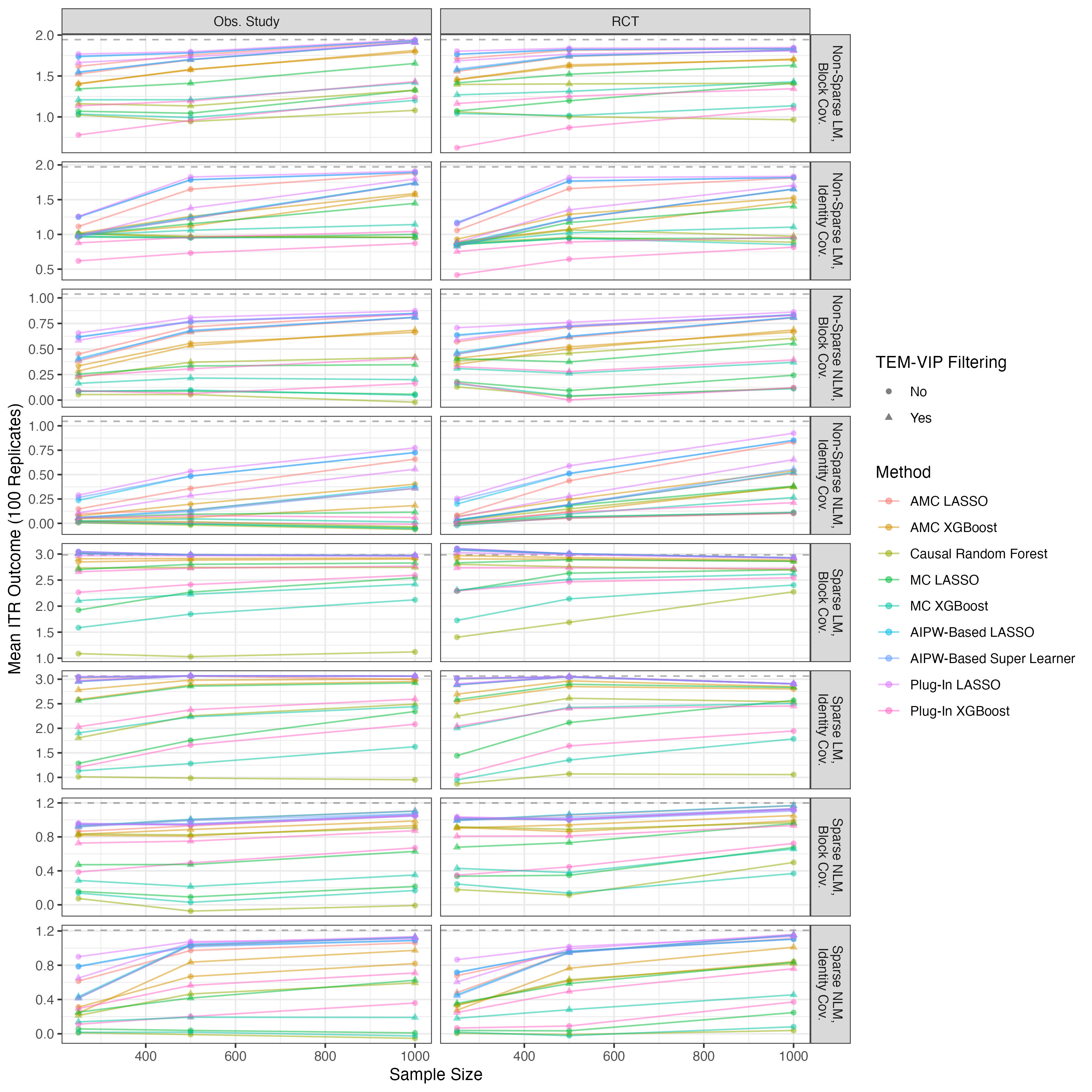
Figure 1: Accuracy: Mean ITR outcome computed over the 100 test set replicates vs. sample size, for each combination of DGP. The dotted line corresponds to the mean outcome under the optimal ITR defined in Proposition 1, which is approximated using a Monte Carlo procedure for each DGP.

Accuracy:

No estimator uniformly dominates the others (Figure 1). In the DGPs with sparse TEMs—regardless of whether treatment is randomized or of the covariates’ correlation structure—the filtered and non-filtered versions of the LASSO-based plug-in, AIPW-based, and augmented modified covariates estimators are the top performers. These estimators produce empirical means that are approximately equal to the population mean under the optimal ITR in the linear model DGPs at all sample sizes and in the non-linear DGPs when $n=1,\!000$. When $n=250$, the non-filtered versions of these estimators generally perform marginally better than their filtered counterparts (Figure A1). The reverse is true as sample size increases.

In the non-sparse settings, the non-filtered plug-in LASSO, AIPW-based, and LASSO-based augmented modified covariates estimators produce the best empirical mean outcomes on average (Figures 1, A1). The empirical means obtained under these estimators are near the population mean under the optimal ITRs as sample size increases. The performance of the filtered versions of these estimators’ generally converges with increasing sample size to that of their non-filtered counterparts. An exception to this trend is observed in the DGPs with non-linear conditional expected outcomes and whose covariates’ covariance matrix is $I_{500\times 500}$.

The XGBoost-based plug-in, modified covariates, and Causal Random Forest estimators are generally less accurate than other estimators considered here, though their performance is improved by the covariate filtering procedure.

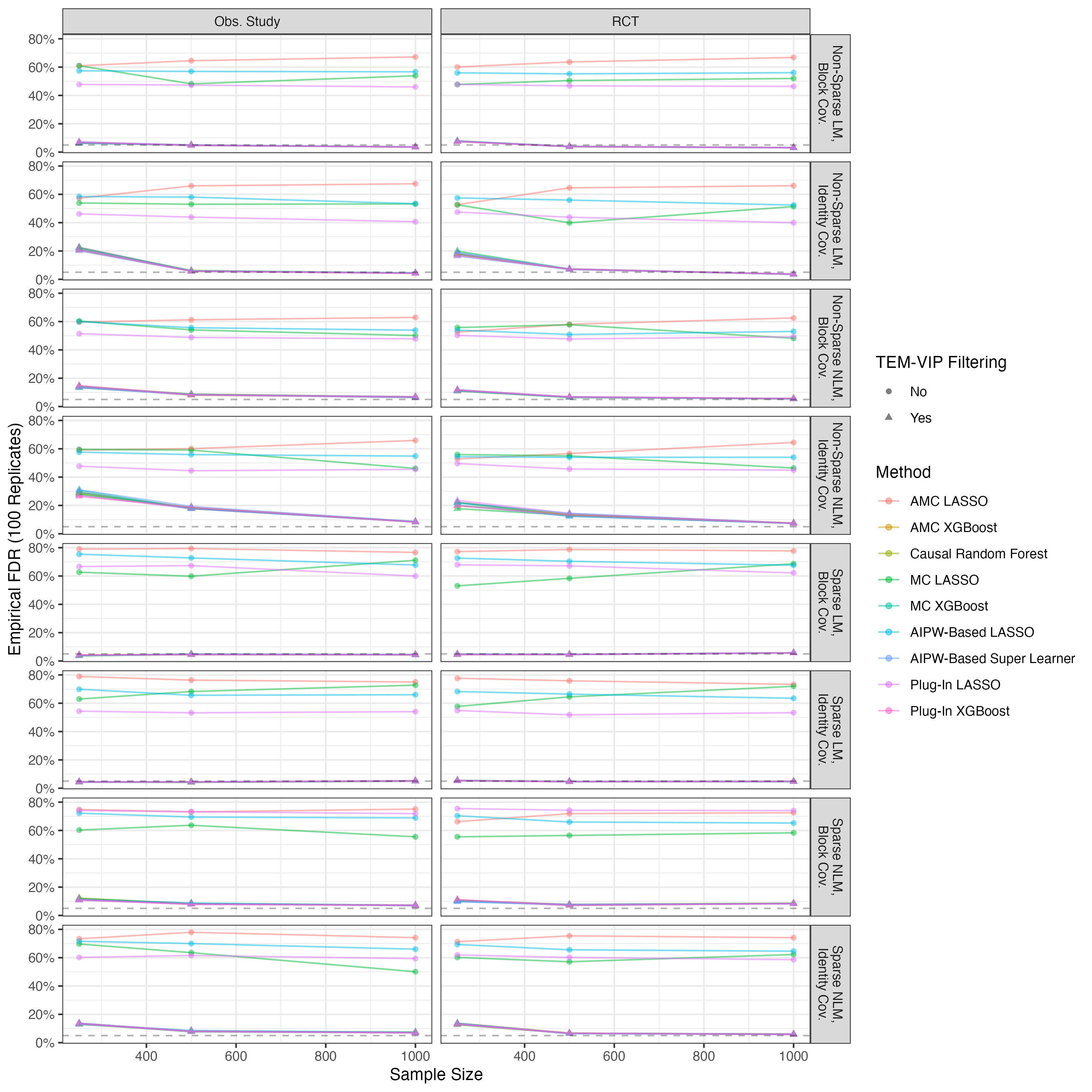
Figure 2: Interpretability, FDR: Empirical FDR computed over the 100 learning set replicates vs. sample size for each combination of DGP. The dotted line corresponds to desired nominal Type I error rate of $5\%$.

Interpretability:

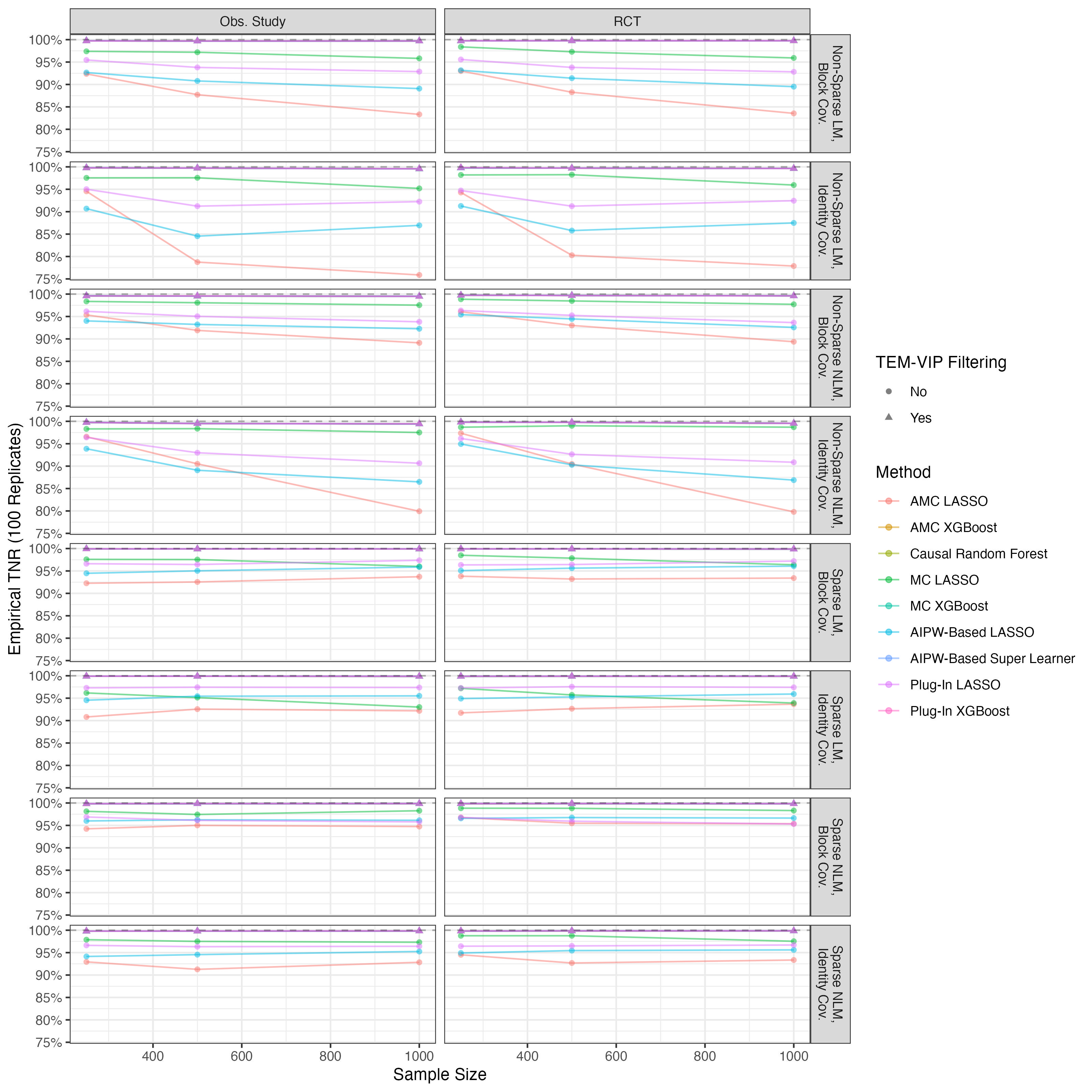
Figure A3: Interpretability, TNR: Empirical TNR computed over the 100 learning set replicates vs. sample size for each combination of DGP. The dotted line corresponds to desired TNR of $100\%$.

As illustrated in Boileau et al. (2022, 2023), only ITR estimators employing the TEM-VIP-based filtering procedure reliably control the FDR near the nominal $5\%$ level regardless of the treatment assignment mechanism (Figure 2). Indeed, these estimators produce empirical FDR equal to $\approx 5\%$ in all DGPs for sample sizes equal to or larger than $500$. All other estimators capable of classifying TEMs produce empirical FDRs ranging from $40\%$ to $80\%$. However, we find that this FDR control sometimes results in a worse empirical TPR in non-sparse settings (Figure A2). With respect to the empirical TNR, only the filtered estimators produce near-perfect results, and this regardless of sample size (Figure A3).

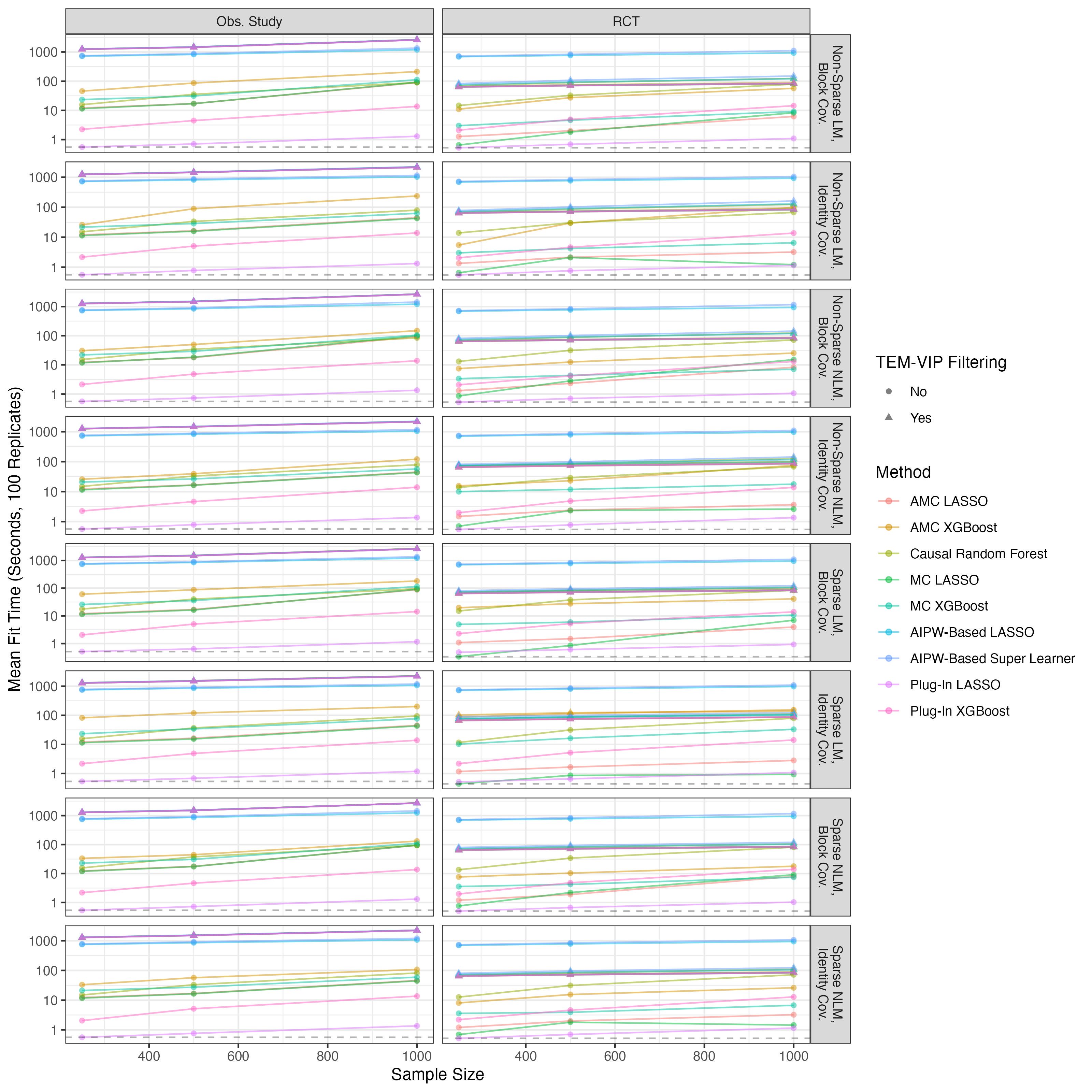
Figure 3: Computational Efficiency: Fit time computed over the 100 learning set replicates vs. sample size for each combination of DGP. The dotted line corresponds to the minimum mean fit time observed in each DGP.

Computational Efficiency:

In RCT DGPs, the non-filtered LASSO-based plug-in estimator generally has the lowest mean fit time across all sample sizes and DGPs, followed closely by the non-filtered (augmented) modified covariates estimators using the LASSO and the non-filtered XGBoost plug-in estimator (Figure 3). The non-filtered AIPW-based estimators are the slowest estimators to produce a rule in all DGPs and sample sizes. All estimators using the TEM-VIP-based filtering procedure exhibit similar mean fit times that are several orders of magnitude larger than that of the non-filtered LASSO-based plug-in estimator. These filtered estimators’ mean fit times are sometimes similar, however, to their non-filtered counterparts when $n=1,\!000$, as is the case with Causal Random Forests and the augmented modified covariates estimators using XGBoost. Further, the filtered AIPW-based estimators have lower mean fit times than their non-filtered versions.

Similar patterns are observed in the observational study DGPs’ simulations. The non-filtered plug-in estimator using the LASSO is again the most computationally efficient procedure, followed by the non-filtered plug-in estimator using XGBoost (Figure 3). The non-filtered (augmented) modified covariates estimators and non-filtered the Causal Random Forests exhibit similar mean fit times which are approximately two orders of magnitude larger than the fastest estimator. The nonparametric AIPW-based estimators are again the slowest of the non-filtered estimators, though they produce estimated rules more quickly than any of the estimators relying on the TEM-VIP-based filtering strategy.

5 Discussion

The simulation results suggest that no ITR estimator uniformly dominates all others with respect to accuracy, interpretability, and computational efficiency in the continuous outcome, binary treatment setting. We posit that the same is true in binary outcome, binary treatment settings. A trade-off must therefore be made when selecting a method with which to learn a treatment rule. Given that the primary goal of learning an ITR is to optimize patient benefit—that is, to learn the optimal ITR—we hold that only accurate estimators should be considered. Selecting a procedure therefore comes down to favoring either interpretability or computational efficiency as a secondary goal.

If more importance is placed on interpretability than computational efficiency, the TEM-VIP-based filtering procedure is a virtual necessity. None of the non-filtered estimators considered here reliably control the empirical FDR or produce near-perfect empirical TPRs (Figures 2, A3). Even when empirical TPR optimization is required, filtered estimators generally perform as well as non-filtered estimators (Figure A2). In sparse TEM scenarios, the most accurate estimators are generally filtered (Figure A1). In non-sparse TEM settings, the filtered LASSO-based plug-in and AIPW-based estimators are typically only marginally worse than the most accurate non-filtered estimators.

However, the use of this filtering procedure may be constrained by available computing power. In RCTs, this filtering procedure makes fitting ITR estimators slower than their non-filtered versions in small sample sizes (Figure 3)—with the exception of the AIPW-based ITR estimators. However, this gap decreases in larger sample sizes: the mean fit times for the filtered estimators are approximately constant, while the non-filtered estimators’ fit times follow an approximately exponential function of sample size. In observational studies, where more computationally intensive nuisance parameter estimators are generally required to ensure reliable TEM classification, the filtered estimators are generally several orders of magnitude slower than their non-filtered counterparts.

When there is limited time, effort, or computing resources available to learn an ITR, the simulation study results suggest that the non-filtered LASSO-based plug-in estimator or the non-filtered augmented modified covariates approach using XGBoost should be used for analyzing data collected in an RCT. In observational studies, the LASSO-based plug-in estimator is the most computationally efficient of the sufficiently accurate estimators. We again emphasize, however, that the computational efficiency of these procedures comes at the cost interpretability: these estimators cannot reliably distinguish TEMs from non-modifiers.

6 Recommendations

We summarize our discussion of the simulation results with concise recommendations about the choice of ITR estimators based on desired operating characteristics.

Accurate and interpretable:

The filtered LASSO-based plug-in and AIPW-based estimators generally produce accurate ITR estimates while reliably recovering TEMs. These estimators are computationally intensive, however. When computational resources are available, parallelized implementations of these estimators will decrease the time required to produce a treatment rule estimate.

Accurate and computationally efficient:

The LASSO-based plug-in estimator is among the most accurate in our simulation study, providing empirical evidence that it is robust to model misspecification while being exceptionally computationally efficient. However, as previously mentioned, this estimator’s built-in feature selection capabilities should not be used for TEM recovery.

We emphasize that while this simulation study is comprehensive, practitioners may nevertheless benefit from performing bespoke benchmarks of their own. The code used to generate the simulations results of Section 4, found on GitHub, may serve as foundation for extensions and modifications.

Code

Code used to generate the results is available in the PhilBoileau/pub_guidance-on-ITR-estimation-in-HD GitHub repository.

Appendix

Figure A1: Accuracy: Mean ITR outcome ranks computed over the 100 test set replicates vs. sample size for each combination of DGP. The dotted line corresponds to the desired rank, one.

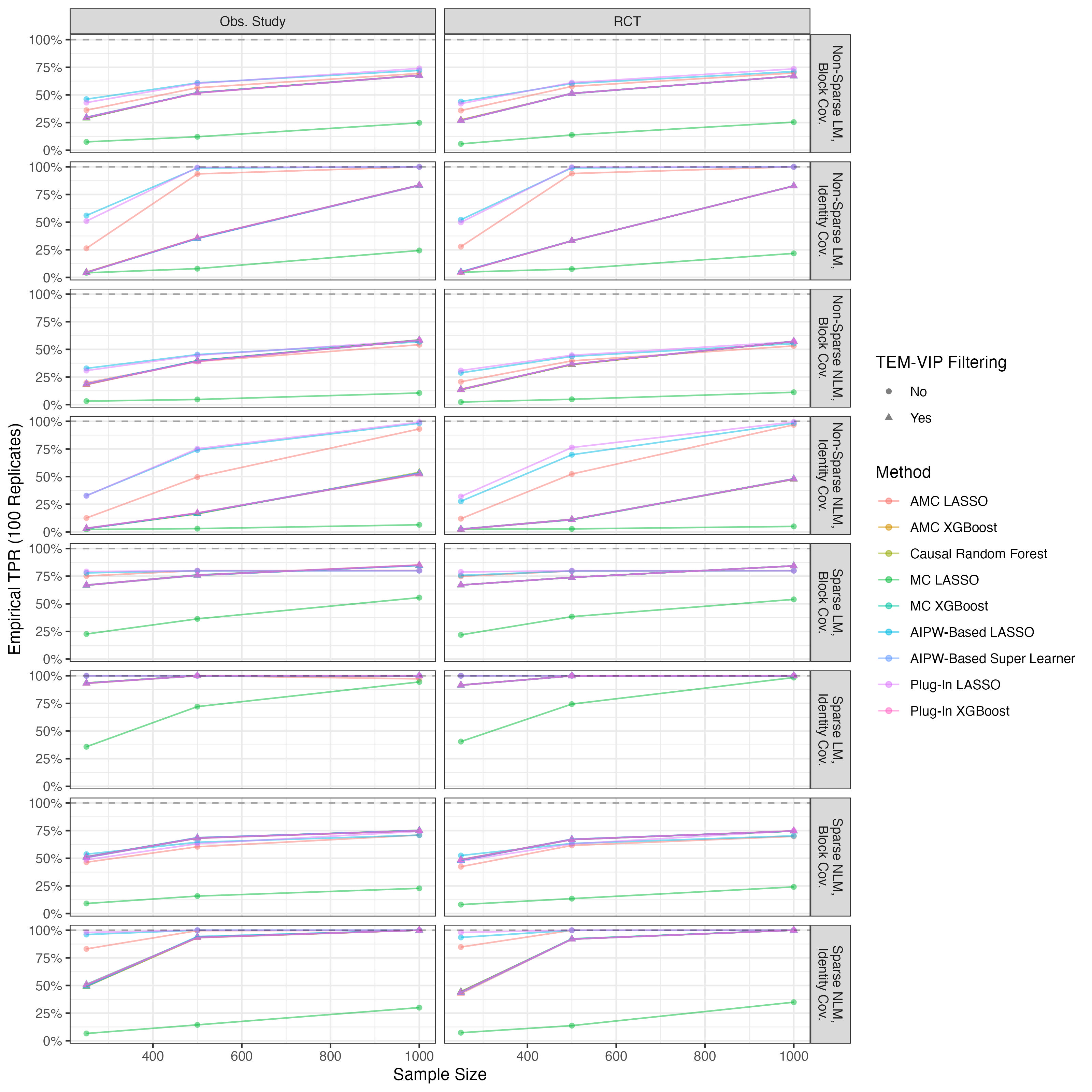
Figure A2: Interpretability, TPR: Empirical TPR computed over the 100 learning set replicates vs. sample size for each combination of DGP. The dotted line corresponds to desired TPR of $100\%$.

References

- Athey et al. [2019] S. Athey, J. Tibshirani, and S. Wager. Generalized random forests. The Annals of Statistics, 47(2):1148–1178, 4 2019.
- Bahamyirou et al. [2022] A. Bahamyirou, M. E. Schnitzer, E. H. Kennedy, L. Blais, and Y. Yang. Doubly robust adaptive lasso for effect modifier discovery. The International Journal of Biostatistics, 2022. doi: doi:10.1515/ijb-2020-0073. URL https://doi.org/10.1515/ijb-2020-0073.
- Benjamini and Hochberg [1995] Y. Benjamini and Y. Hochberg. Controlling the false discovery rate: A practical and powerful approach to multiple testing. Journal of the Royal Statistical Society. Series B (Methodological), 57(1):289–300, 1995. ISSN 00359246. URL http://www.jstor.org/stable/2346101.
- Boileau et al. [2022] P. Boileau, N. T. Qi, M. J. van der Laan, S. Dudoit, and N. Leng. A flexible approach for predictive biomarker discovery. Biostatistics, 07 2022. ISSN 1465-4644. doi: 10.1093/biostatistics/kxac029. URL https://doi.org/10.1093/biostatistics/kxac029. kxac029.
- Boileau et al. [2023] P. Boileau, N. Leng, N. S. Hejazi, M. van der Laan, and S. Dudoit. A nonparametric framework for treatment effect modifier discovery in high dimensions, 2023.
- Breiman [2001] L. Breiman. Random forests. Machine Learning, 45(1):5–32, 2001.
- Chen et al. [2017] S. Chen, L. Tian, T. Cai, and M. Yu. A general statistical framework for subgroup identification and comparative treatment scoring. Biometrics, 73(4):1199–1209, 2017. doi: https://doi.org/10.1111/biom.12676. URL https://onlinelibrary.wiley.com/doi/abs/10.1111/biom.12676.
- Chen and Guestrin [2016] T. Chen and C. Guestrin. XGBoost: A scalable tree boosting system. In Proceedings of the 22nd ACM SIGKDD International Conference on Knowledge Discovery and Data Mining, KDD ’16, pages 785–794, New York, NY, USA, 2016. ACM. ISBN 978-1-4503-4232-2. doi: 10.1145/2939672.2939785. URL http://doi.acm.org/10.1145/2939672.2939785.
- Coyle et al. [2021] J. R. Coyle, N. S. Hejazi, I. Malenica, R. V. Phillips, and O. Sofrygin. sl3: Modern Pipelines for Machine Learning and Super Learning, 2021. URL https://doi.org/10.5281/zenodo.1342293. R package version 1.4.2.
- Dudoit and van der Laan [2003] S. Dudoit and M. J. van der Laan. Asymptotics of cross-validated risk estimation in estimator selection and performance assessment. Working Paper 126, University of California, Berkeley, Berkeley, 2003. URL https://biostats.bepress.com/ucbbiostat/paper126.
- Dudoit and van der Laan [2005] S. Dudoit and M. J. van der Laan. Asymptotics of cross-validated risk estimation in estimator selection and performance assessment. Statistical Methodology, 2(2):131–154, 2005.
- Huling and Yu [2021] J. D. Huling and M. Yu. Subgroup identification using the personalized package. Journal of Statistical Software, 98(5):1–60, 2021. doi: 10.18637/jss.v098.i05. URL https://www.jstatsoft.org/index.php/jss/article/view/v098i05.
- Kennedy [2022] E. H. Kennedy. Towards optimal doubly robust estimation of heterogeneous causal effects, 2022.
- Künzel et al. [2019] S. R. Künzel, J. S. Sekhon, P. J. Bickel, and B. Yu. Metalearners for estimating heterogeneous treatment effects using machine learning. Proceedings of the National Academy of Sciences, 116(10):4156–4165, 2019.
- Luedtke and van der Laan [2016] A. R. Luedtke and M. J. van der Laan. Super-learning of an optimal dynamic treatment rule. The International Journal of Biostatistics, 12(1):305–332, 2016. doi: doi:10.1515/ijb-2015-0052. URL https://doi.org/10.1515/ijb-2015-0052.
- Murdoch et al. [2019] W. J. Murdoch, C. Singh, K. Kumbier, R. Abbasi-Asl, and B. Yu. Definitions, methods, and applications in interpretable machine learning. Proceedings of the National Academy of Sciences, 116(44):22071–22080, 2019.
- Qian and Murphy [2011] M. Qian and S. A. Murphy. Performance guarantees for individualized treatment rules. The Annals of Statistics, 39(2):1180 – 1210, 2011. doi: 10.1214/10-AOS864. URL https://doi.org/10.1214/10-AOS864.
- R Core Team [2021] R Core Team. R: A Language and Environment for Statistical Computing. R Foundation for Statistical Computing, Vienna, Austria, 2021. URL https://www.R-project.org/.
- Robins et al. [2008] J. Robins, L. Orellana, and A. Rotnitzky. Estimation and extrapolation of optimal treatment and testing strategies. Statistics in Medicine, 27(23):4678–4721, 2008. doi: https://doi.org/10.1002/sim.3301. URL https://onlinelibrary.wiley.com/doi/abs/10.1002/sim.3301.
- Robins [2004] J. M. Robins. Optimal Structural Nested Models for Optimal Sequential Decisions, pages 189–326. Springer New York, New York, NY, 2004.
- Robinson [1988] P. M. Robinson. Root-n-consistent semiparametric regression. Econometrica, 56:931–954, 1988.
- Rubin [1974] D. Rubin. Estimating causal effects of treatments in randomized and nonrandomized studies. Journal of Educational Psychology, 66(5):688–701, 1974.
- Tian et al. [2014] L. Tian, A. A. Alizadeh, A. J. Gentles, and R. Tibshirani. A simple method for estimating interactions between a treatment and a large number of covariates. Journal of the American Statistical Association, 109(508):1517–1532, 2014. doi: 10.1080/01621459.2014.951443. URL https://doi.org/10.1080/01621459.2014.951443. PMID: 25729117.
- Tibshirani et al. [2022] J. Tibshirani, S. Athey, E. Sverdrup, and S. Wager. grf: Generalized Random Forests, 2022. URL https://CRAN.R-project.org/package=grf. R package version 2.2.1.
- Tibshirani [1996] R. Tibshirani. Regression shrinkage and selection via the lasso. Journal of the Royal Statistical Society. Series B (Methodological), 58(1):267–288, 1996. ISSN 00359246. URL http://www.jstor.org/stable/2346178.
- van der Laan and Dudoit [2003] M. J. van der Laan and S. Dudoit. Unified cross-validation methodology for selection among estimators and a general cross-validated adaptive epsilon-net estimator: Finite sample oracle inequalities and examples. Working Paper 130, University of California, Berkeley, Berkeley, 2003. URL https://biostats.bepress.com/ucbbiostat/paper130/.
- van der Laan and Luedtke [2015] M. J. van der Laan and A. R. Luedtke. Targeted learning of the mean outcome under an optimal dynamic treatment rule. Journal of Causal Inference, 3(1):61–95, 2015. doi: doi:10.1515/jci-2013-0022. URL https://doi.org/10.1515/jci-2013-0022.
- van der Laan et al. [2007] M. J. van der Laan, E. C. Polley, and A. E. Hubbard. Super learner. Statistical Applications in Genetics and Molecular Biology, 6(1), 2007. doi: doi:10.2202/1544-6115.1309. URL https://doi.org/10.2202/1544-6115.1309.
- van der Vaart et al. [2006] A. W. van der Vaart, S. Dudoit, and M. J. van der Laan. Oracle inequalities for multi-fold cross validation. Statistics and Decisions, 24:351–371, 2006.
- Wager and Athey [2018] S. Wager and S. Athey. Estimation and inference of heterogeneous treatment effects using Random Forests. Journal of the American Statistical Association, 113(523):1228–1242, 2018. doi: 10.1080/01621459.2017.1319839. URL https://doi.org/10.1080/01621459.2017.1319839.
- Zhang et al. [2012a] B. Zhang, A. A. Tsiatis, M. Davidian, M. Zhang, and E. Laber. Estimating optimal treatment regimes from a classification perspective. Stat, 1(1):103–114, 2012a. doi: https://doi.org/10.1002/sta.411. URL https://onlinelibrary.wiley.com/doi/abs/10.1002/sta.411.
- Zhang et al. [2012b] B. Zhang, A. A. Tsiatis, E. B. Laber, and M. Davidian. A robust method for estimating optimal treatment regimes. Biometrics, 68(4):1010–1018, 2012b. doi: https://doi.org/10.1111/j.1541-0420.2012.01763.x. URL https://onlinelibrary.wiley.com/doi/abs/10.1111/j.1541-0420.2012.01763.x.
- Zhao and Yu [2006] P. Zhao and B. Yu. On model selection consistency of lasso. Journal of Machine Learning Research, 7(90):2541–2563, 2006. URL http://jmlr.org/papers/v7/zhao06a.html.
- Zhao et al. [2017] Q. Zhao, D. S. Small, and A. Ertefaie. Selective inference for effect modification via the lasso, 2017. URL https://arxiv.org/abs/1705.08020.
- Zou and Hastie [2005] H. Zou and T. Hastie. Regularization and variable selection via the elastic net. Journal of the Royal Statistical Society: Series B (Statistical Methodology), 67(2):301–320, 2005.