Dirac materials in parallel non-uniform electromagnetic fields generated by SUSY:
A new class of chiral Planar Hall Effect?

Abstract

Within a Supersymmetric Quantum Mechanics (SUSY-QM) framework, the (3+1) Dirac equation describing a Dirac material in the presence of external parallel electric and magnetic fields is solved. Considering static but non-uniform electric and magnetic profiles with translational symmetry along the $y$-direction, the Dirac equation is transformed into two decoupled pairs of Schrödinger equations, one for each chirality of the fermion fields. Taking trigonometric and hyperbolic profiles for the vector and scalar potentials, respectively, we arrive at SUSY partner Pöschl-Teller-like quantum potentials. Restricting to the conditions of the potentials that support an analytic zero-mode solution, we obtain a nontrivial current density in the same plane where the electric and magnetic fields lie, but perpendicular to both of them, indicating the possibility of realizing the Planar Hall Effect. Furthermore, this non-vanishing current density is the sum of current densities for the left- and right-chiralities, suggesting that the net current is a consequence of chiral symmetry.

I Introduction

Understanding the dynamics of electrons under the influence of external electromagnetic fields lies at the very heart of quantum mechanics [1, 2, 3]. Not surprisingly, the influence of external fields results in a plethora of quantum phenomena. Addressing the problem under the most general assumptions regarding field configurations is indeed a hard nut to crack. A number of simplifications have been considered since the early days of the establishment of quantum physics. For example, for static fields, the quantization of electron orbitals in the plane perpendicular to the field lines of a uniform magnetic field, the Landau levels [4], are the cornerstone in the description of several quantum phenomena [5]. Adding an electric field parallel to the Landau levels plane generates an electric current perpendicular to both fields. For finite size samples, the quantization of the electric resistance is observed in the Quantum Hall effect (QHE) [6, 7] whose smoking gun is the development of plateaus in the transverse conductivity of a bi-dimensional sample of a two-dimensional electron gas at integer numbers of the so-called filling factor, which counts the number of Landau levels filled in the sample. The quantization rule for the conductivity has also been found for non-integer values of the filling factor [8] as a result of electron-electron interactions which become relevant [9]. Even more, in the anomalous quantum Hall effect [10, 11, 12] which emerges for relativistic-like excitations in graphene and related materials, it is precisely the relativistic nature of the excitations which describes a sort of integer QHE, with a shifted plateaus. This particular example establishes a natural connection of condensed matter and high-energy physics [13]. The importance of the QHE can be further established by the close relation of this effect and the superconducting properties of spin liquid systems [14]. Thus, it is natural to expect the response of charged particles to external fields in variants of this effect.

For time varying fields, like those generated during relativistic heavy-ion collisions in RHIC and LHC [15], it was conjectured that the non-trivial nature of the quantum chromodynamics vacuum could be probed through the generation of a non-dissipative electric current generated by the chiral imbalance of quarks interacting with topological sectors of the gauge field [16, 17, 18]. Chiral anomaly is responsible for the imbalance in this effect. Nevertheless, a number of thorough measurements in isobaric collisions showed no evidence of the chiral magnetic effect (CME) [19, 20]. An (Abelian) analog of the CME was found in ZrTe₅ [21, 22, 23, 24]. In this case, rather than topological configurations of the gauge fields, it is a setup where electric and magnetic fields are parallel which is responsible for the effect. Remarkably, the chiral anomaly generated by the effect of parallel electric and magnetic fields has also been related to the emergence of a positive longitudinal magnetoconductance [25] in Dirac materials. Along with non-trivial effects of Berry curvature, the chiral anomaly also gives rise to the so-called Planar Hall Effect (PHE) [26] that contrary to the standard QHE setup, in this case the applied current, magnetic field, and the transverse voltage lie coplanarly.

In this work we explore the possibility of realizing the PHE by static but non-uniform electric and magnetic fields, as can be naturally addressed in the context of $\theta$-electrodynamics (see, for instance, Ref. [27]). For this purpose, we factorize the four-component Dirac equation under the influence of parallel electric and magnetic fields along the third spatial dimension in terms of two decoupled two-component Weyl-type equation corresponding to each chirality. Each bi-spinor equation can be further factorized in the standard procedure of supersymmetric quantum mechanics. Considering Pöschl-Teller-like quantum potentials, we look for the conditions of these potentials to support a zero-mode analytic solution. Interestingly, this mode leads to a nontrivial electric current in the same plane of the electric and magnetic field, but perpendicular to both. To present the details of our findings, we have organized the remaining of this article as follows: In Sec. II we recall the covariant form of the (3+1) Dirac equation in the presence of external electromagnetic fields. Later, in Sec. III, we consider a confining example of scalar and vector potentials which leads to a novel chiral Planar Hall Effect. Finally, in Sec. IV we discuss some aspects and consequences of the aforementioned effect and draw some conclusions.

II Dirac equation in electromagnetic fields

The Dirac equation describing the motion of free electrons is given by

$$(i\gamma^{\mu}\partial_{\mu}-m)\Psi_{D}(\mathbf{x})=0,$$ (1)

where $\Psi_{D}(\mathbf{x})$ is a four-component spinor, and the Dirac $\gamma^{\mu}$-matrices fulfill the Clifford algebra $\{\gamma^{\mu},\gamma^{\nu}\}=2g^{\mu\nu}$, with $g^{\mu\nu}=\rm{diag}(1,-1,-1,-1)$ being the (3+1)-dimensional Minkowsky space-time metric. We choose to work in the Dirac representation of these matrices,

$$\gamma^{0}=\beta=\begin{pmatrix}1&0\\ 0&-1\\ \end{pmatrix},~{}\gamma^{i}=\beta\alpha_{i}=\begin{pmatrix}0&\sigma_{i}\\ -\sigma_{i}&0\\ \end{pmatrix},$$

$$\alpha_{i}=\begin{pmatrix}0&\sigma_{i}\\ \sigma_{i}&0\\ \end{pmatrix},~{}\gamma^{5}=i\gamma^{0}\gamma^{1}\gamma^{2}\gamma^{3}=\begin{pmatrix}0&1\\ 1&0\\ \end{pmatrix}.$$ (2)

It is worth noticing that we are working in natural units $\hbar=c=e=1$, where $c$ is the speed of light and $e$ is the electron charge. However, in Dirac materials, the Dirac-like equation describing them has a factor directly proportional to the Fermi velocity $v_{F}$ instead of $c$ (see for example [28]), thus, the system addressed here is not relativistic. In order to formulate the Dirac equation in the presence of electromagnetic fields, we start by taking the minimal coupling rule $\pi_{\mu}=i\partial_{\mu}-A_{\mu}$ which incorporates the electromagnetic potentials $A_{\mu}=(\Phi,\mathbf{A})$ in the Dirac equation. Thus, Eq. (1) becomes

$$(\gamma^{\mu}\pi_{\mu}-m)\Psi_{D}(\mathbf{x})=0.$$ (3)

Considering the massless case, it is easy to show that the squared operator $(\gamma\cdot\pi)^{2}$ can be written as follows

$$(\bm{\gamma}\cdot\bm{\pi})^{2}=\pi^{2}+\frac{\sigma^{\mu\nu}}{2}F_{\mu\nu},$$ (4)

where $\sigma^{\mu\nu}=\frac{i}{2}[\gamma^{\mu},\gamma^{\nu}]$, and

$$F_{\mu\nu}=[\pi_{\mu},\pi_{\nu}]=\begin{pmatrix}0&&E_{x}&&E_{y}&&E_{z}\\ -E_{x}&&0&&-B_{z}&&B_{y}\\ -E_{y}&&B_{z}&&0&&-B_{x}\\ -E_{z}&&-B_{y}&&B_{x}&&0\end{pmatrix},$$ (5)

is the electromagnetic field tensor [29]. Let us analyse each term in Eq. (4) separately. First,

$$\pi^{2} = -\partial_{t}^{2}-i\frac{\partial A_{0}}{\partial t}-2iA_{0}\partial_{t}+A_{0}^{2}+\partial_{j}^{2}$$ (6)

$$+i\frac{\partial A_{j}}{\partial x^{j}}+2iA_{j}\partial_{j}-A_{j}^{2}.$$

On the other hand, noticing that

$$\frac{\sigma^{0\nu}}{2}F_{0\nu} =\frac{i}{2}\alpha_{i}F_{0i}$$

$$=\frac{i}{2}(\alpha_{1}F_{01}+\alpha_{2}F_{02}+\alpha_{3}F_{03}),$$ (7)

$$\frac{\sigma^{ij}}{2}F_{ij} =-\frac{1}{2}\epsilon_{ijk}F_{ij}I\otimes\sigma_{k}$$

$$=-I\otimes(\sigma_{3}F_{12}-\sigma_{2}F_{13}+\sigma_{1}F_{23}),$$ (8)

where $I=I_{2\times 2}$ is the identity matrix, the second term can be written as

$$\frac{\sigma^{\mu\nu}}{2}F_{\mu\nu} = \frac{i}{2}(\alpha_{1}F_{01}+\alpha_{2}F_{02}+\alpha_{3}F_{03})$$ (9)

$$- I\otimes(\sigma_{3}F_{12}-\sigma_{2}F_{13}+\sigma_{1}F_{23}),$$

where we have used the relations $[\gamma^{0},\gamma^{i}]=2\alpha_{i}$, $[\gamma^{i},\gamma^{j}]=i2\epsilon_{ijk}\sigma_{k}\otimes I_{2\times 2}$, $F_{\mu\nu}=-F_{\nu\mu}$ and $\sigma^{\mu\nu}=-\sigma^{\nu\mu}$. Equation (4) together with the expressions in Eqs. (6) and (9) represent all the possible configurations of electromagnetic fields coupled to the Dirac equation describing the dynamics of fermions under its influence. In particular, we are interested in configurations allowing the use of the Supersymetric Quantum Mechanics (SUSY-QM) to solve the eigenvalue problem of the Dirac Hamiltonian. It has been demonstrated that when we only consider a magnetic field perpendicular to the $X-Y$ plane, where fermions are constrained to move, the system can be solved within a SUSY framework (see, for example, Ref. [30]). Analogously, in the case of an electric field pointing along the $X$-direction, SUSY-QM is also a framework useful to find the respective solutions [31]. On the other hand, from Eq. (9) we observe that a configuration of magnetic and electric fields does not lead to a system of equations which can be solved by a suitable SUSY-QM. Below we study a particular setup in which the system exhibits supersymmetry.

II.1 Parallel electromagnetic fields

Let us consider a static parallel fields configuration, namely, a magnetic field $\mathbf{B}=B(x)\ \mathbf{\hat{z}}$ and an electric field $\mathbf{E}=E(z)\ \mathbf{\hat{z}}$. Working in the Landau gauge, the vector potential generating $\mathbf{B}$ can be chosen as $\mathbf{A}=A(x)\ \mathbf{\hat{y}}$. Moreover, since the rotational of the electric field is equal to zero, this field is generated by a electric scalar potential $\phi(z)$. Thus, the field strengths turn out to be

$$B(x)=\frac{dA(x)}{dx},\quad E(z)=-\frac{d\phi(z)}{dz}.$$ (10)

In this physical situation, the operator $\pi^{2}$ is simplified to the following form

$$\pi^{2}= -\partial^{2}_{t}-i2\phi(z)\partial_{t}+\phi^{2}(z)+\partial^{2}_{x}+\partial^{2}_{y}+\partial^{2}_{z}$$ (11)

$$+i2A(x)\partial_{y}-A^{2}(x),$$

while the term $\sigma^{\mu\nu}F^{\mu\nu}/2$ is explicitly written as

$$\frac{\sigma^{\mu\nu}}{2}F^{\mu\nu}=\begin{pmatrix}B(x)&&0&&iE(z)&&0\\ 0&&-B(x)&&0&&-iE(z)\\ iE(z)&&0&&B(x)&&0\\ 0&&-iE(z)&&0&&-B(x)\end{pmatrix}.$$ (12)

On the other hand, we assume the spinor $\Psi_{D}(t,x,y,z)$, such that $(\gamma\cdot\pi)^{2}\Psi_{D}(t,x,y,z)=0$, has a standard stationary temporal behavior and since the system exhibits translational symmetry along the $Y$-direction, we propose $\Psi_{D}(t,x,y,z)$ as follows,

$$\Psi_{D}(t,x,y,z)=e^{i(\varepsilon t+ky)}\Psi(x,z)=e^{i(\varepsilon t+ky)}\begin{pmatrix}\psi^{\alpha}_{\uparrow}\\ \psi^{\beta}_{\downarrow}\\ \psi^{\beta}_{\uparrow}\\ \psi^{\alpha}_{\downarrow}\end{pmatrix},$$ (13)

with $\varepsilon$ being the energy of the Dirac electron and $k$ its wavenumber in the $Y$-direction. Then, the time-independent spinor $\Psi(x,z)$ fulfills an eigenvalue problem that is equivalent to the following coupled system of equations

$$\left\{\left[\partial_{x}^{2}-(k+A(x))^{2}\pm\frac{dA(x)}{dx}\right]+\left[\partial_{z}^{2}+(\phi(z)+\varepsilon)^{2}\right]\right\}\psi_{\uparrow\downarrow}^{\alpha,\beta}\mp i\frac{d\phi(z)}{dz}\psi_{\uparrow\downarrow}^{\beta,\alpha}=0,$$ (14)

where the arrows $\uparrow\downarrow$ specify the spin orientation. The above system can be decoupled defining

$$\varphi^{\pm}_{\uparrow\downarrow}\equiv\psi^{\alpha}_{\uparrow\downarrow}\pm\psi^{\beta}_{\uparrow\downarrow},\quad$$ (15)

such that we are lead to the following system of equations

$$\left[\left(-\partial_{x}^{2}+(k+A(x))^{2}-\frac{dA(x)}{dx}\right)\right.$$

$$+\left.\left(-\partial_{z}^{2}-(\phi(z)+\varepsilon)^{2}\pm i\frac{d\phi(z)}{dz}\right)\right]\varphi^{\pm}_{\uparrow}=0,$$ (16a)

$$\left[\left(-\partial_{x}^{2}+(k+A(x))^{2}+\frac{dA(x)}{dx}\right)\right.$$

$$+\left.\left(-\partial_{z}^{2}-(\phi(z)+\varepsilon)^{2}\mp i\frac{d\phi(z)}{dz}\right)\right]\varphi^{\pm}_{\downarrow}=0.$$ (16b)

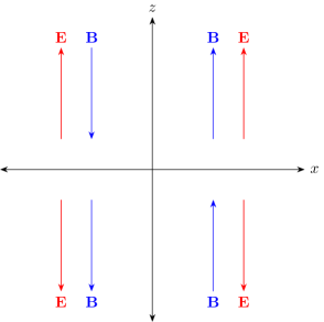
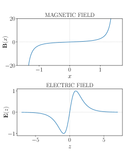
Figure 1: A sketch of the alignment of the fields in the plane X-Z (left). The electromagnetic fields generated by the potentials in Eq. (26) (right). The scale of the graphs is set by parameters $E_{0}=2.0$, $B_{0}=1.0$, $\mu=1.0$ and $\nu=1.0$.

Before proceeding, let us briefly review the SUSY-QM framework, in which two Schrödinger-like Hamiltonians $H^{\pm}$ are intertwined by means of the operational relation

$$H^{+}L^{-}=L^{-}H^{-},$$ (17)

with $L^{-}$ being the intertwining operator given by

$$L^{-}=\frac{d}{dx}+w(x),$$ (18)

where $w(x)$ is a real function referred to as the superpotential. Within, the SUSY-QM framework, the partner potentials $V^{\pm}$ associated to the intertwined Hamiltonians $H^{\pm}$ can be written in terms of the superpotential function as follows

$$V^{\pm}=w^{2}(x)\pm w^{\prime}(x).$$ (19)

Consequently, both Hamiltonians have an isospectral part and their eigenfunctions are linked through the supersymmetric transformation defined by the intertwining operator [32, 33, 34]. The SUSY algorithm has been successfully applied to solve the Dirac equation [35, 36], in particular, when this equation describes Dirac materials such as graphene [30, 37, 38, 39].

Defining the Schrödinger-like Hamiltonians

$$H^{\pm}_{A}=-\partial_{x}^{2}+(k+A(x))^{2}\pm\frac{dA(x)}{dx},$$ (20a)

$$H^{\pm}_{\phi}=-\partial_{z}^{2}+[i(\phi(z)+\varepsilon)]^{2}\pm i\frac{d\phi(z)}{dz},$$ (20b)

which are first-order supersymmetric partners, respectively, the corresponding SUSY transformations can be defined by the superpotentials

$$\text{w}_{A}=k+A(x),\quad\text{w}_{\phi}=i(\varepsilon+\phi(z)).$$ (21)

Thus, with the aid of the SUSY algorithm, the system of equations (16) can be written as

$$\left[H^{-}_{A}+H^{\pm}_{\phi}\right]\varphi^{\pm}_{\uparrow}=0,$$ (22a)

$$\left[H^{+}_{A}+H^{\mp}_{\phi}\right]\varphi^{\pm}_{\downarrow}=0.$$ (22b)

Expressions above imply that we can construct solutions of the form

$$\varphi^{\pm}_{\uparrow}=\chi^{-}_{\uparrow}(x)\zeta^{\pm}_{\uparrow}(z),\quad\varphi^{\pm}_{\downarrow}=\chi^{+}_{\downarrow}(x)\zeta^{\mp}_{\downarrow}(z),$$ (23)

satisfying each one an eigenvalue equation of the form

$$H^{\pm}_{A}\chi^{\pm}_{\uparrow\downarrow}=\varepsilon_{A}\chi^{\pm}_{\uparrow\downarrow},\quad H^{\pm}_{\phi}\zeta^{\pm}_{\uparrow\downarrow}=\varepsilon_{\phi}\zeta^{\pm}_{\uparrow\downarrow}.$$ (24)

Hence, we obtain a relation between the energies $\varepsilon_{A}$ and $\varepsilon_{\phi}$, given by

$$\varepsilon_{A}=-\varepsilon_{\phi}.$$ (25)

By solving the time-independent Schrödinger-like equations (24) such that the constraint in Eq. (25) is fulfilled, it is possible to determine the spinor $\Psi_{D}$ satisfying the massless Dirac equation. It is worth mentioning the potentials $V_{\phi}^{\pm}(z)$ corresponding to the Hamiltonians in Eq. (20b) are complex. Since we are looking for real energy eigenvalues, care must be paid in the choice of the electromagnetic profiles. In the following section we discuss an example of electromagnetic fields which lead to solvable Schrödinger-like potentials. We explicitly explore their analytic solutions.

III Confining case: Pöschl-Teller-like potentials

In order to determine the bound states of the Hamiltonians in Eq. (24), let us take electromagnetic potentials of the form

$$A(x)=\frac{B_{0}}{\nu}\sec(\nu x),\ -\frac{\pi}{2}<\nu x<\frac{\pi}{2};~{}\phi(z)=\frac{E_{0}}{\mu}\text{sech}(\mu z).$$ (26)

In Fig. 1 we show the corresponding electric and magnetic fields produced by these potentials.

With the definitions above, from Eqs. (19) and (21), the SUSY partner potentials are

$$V_{A}^{\pm}(x)= k^{2}+2kD_{A}\sec(\nu x)+D_{A}^{2}\sec^{2}(\nu x)$$ (27a)

$$\pm\nu D_{A}\sec(\nu x)\tan(\nu x),$$

$$V_{\phi}^{\pm}(z)= -\varepsilon^{2}-2\varepsilon D_{\phi}\text{sech}(\mu z)-D_{\phi}^{2}\text{sech}^{2}(\mu z)$$ (27b)

$$\mp i\mu D_{\phi}\text{sech}(\mu z)\tanh(\mu z),$$

where $D_{A}=B_{0}/\nu$, $D_{\phi}=E_{0}/\mu$. Notice that the complex potentials in Eq. (27b), taking $\varepsilon=0$, are particular cases of the so-called pseudo-Hermitian operators with real energy eigenvalues [40, 41]. It can be seen that both potentials have a similar form. Thus, we focus on getting the solutions of $V^{\pm}_{\phi}$; the potentials $V^{\pm}_{A}$ can be solved analogously. In Fig. 2, we plot the SUSY partner potentials in Eq. (27).

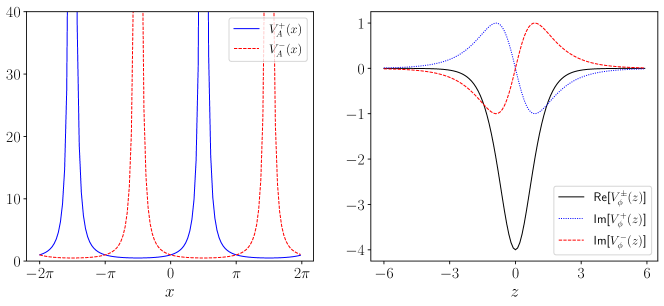
Figure 2: Plot of the Pösch-Teller-like SUSY partner potentials $V^{\pm}_{A}(x)$ (left). Real and imaginary parts of the potentials $V^{\pm}_{\phi}(z)$ (right). The scale of the graphs is set by parameters $E_{0}=2.0$, $B_{0}=1.0$, $\mu=1.0$, $\nu=1.0$ and $\varepsilon=k=0$.

In order to solve the eigenvalue equation of the Hamiltonians $H^{\pm}_{\phi}$, we perform the change of variable $u=i\sinh(\mu z)$, from which we obtain that

$$\left[\mu^{2}(1-u^{2})\frac{d^{2}}{du^{2}}-\mu^{2}u\frac{d}{du}-\varepsilon^{2}-2\frac{\varepsilon D_{\phi}}{\sqrt{1-u^{2}}}-\frac{D_{\phi}^{2}}{1-u^{2}}\mp\mu D_{\phi}\frac{u}{1-u^{2}}-\varepsilon_{\phi}\right]\zeta^{\pm}(u)=0.$$ (28)

Considering $\varepsilon=0$, these differential equations lead to the Jacobi equation. We then propose the wave functions of the form $\zeta^{\pm}(u)=(1-u)^{a}(1+u)^{b}f^{\pm}(u)$. Thus, the differential equations (28) can be written as

$$\left\{(1-u^{2})\frac{d^{2}}{du^{2}}+2[b-a-(b+a+1/2)u]\frac{d}{du}-b(b-1)-a(a-1)-b-a-2ab-\frac{\varepsilon_{\phi}}{\mu^{2}}\right.$$ (29)

$$+\left.\left[2a(a-1)-2b(b-1)-b+a\mp\frac{D_{\phi}}{\mu}\right]\frac{u}{1-u^{2}}+\left[2b(b-1)+2a(a-1)+b+a-\frac{D_{\phi}^{2}}{\mu^{2}}\right]\frac{1}{1-u^{2}}\right\}f^{\pm}(u)=0.$$

Equation (29) accepts as solutions the Jacobi polynomials with complex argument $P_{n}^{(\alpha,\beta)}(u)$ as long as the following conditions are accomplished:

$$2(b-a)=\beta-\alpha,$$

$$2(a+b+1/2)=\alpha+\beta+2,$$

$$-(b+a)^{2}-\frac{\varepsilon_{\phi}}{\mu^{2}}=n(n+\alpha+\beta+1),$$ (30)

$$(a-b)[2(a+b)-1]=\pm S_{\phi},$$

$$2(a^{2}+b^{2})-(a+b)=S^{2}_{\phi},$$

with $S_{\phi}=D_{\phi}/\mu$. Once the above requirements fulfilled, the eigenfunctions of the Hamiltonians $H^{\pm}_{\phi}$ are given by

$$\zeta^{\pm}_{n}(u) =(1-u)^{\frac{1}{4}\left(1-\sqrt{1+4S_{\phi}(S_{\phi}\pm 1)}\right)}$$ (31)

$$\times(1+u)^{\frac{1}{4}\left(1-\sqrt{1+4S_{\phi}(S_{\phi}\mp 1)}\right)}$$

$$\times P_{n}^{\left(-\frac{1}{2}\sqrt{1+4S_{\phi}(S_{\phi}\pm 1)},-\frac{1}{2}\sqrt{1+4S_{\phi}(S_{\phi}\mp 1)}\right)}(u).$$

Boundary conditions imply that $|S_{\phi}|>1$ and a finite discrete spectrum since the number of square-integrable functions is bounded by $Q_{\phi}-1\geq n$, where

$$Q_{\phi}=\frac{\sqrt{1+4S_{\phi}(S_{\phi}+1)}+\sqrt{1+4S_{\phi}(S_{\phi}-1)}}{2}.$$

It is worth-noticing that if $S_{\phi}$ is not an integer, the inequality is strict. Thus, $Q_{\phi}-1$ is a upper value of the number of levels and it is necessary check the square-integrablility of each one of the eigenfunctions. Furthermore, the corresponding eigenvalues are

$$\varepsilon_{\phi}=-\mu^{2}\left[n(n-Q_{\phi}+1)+\frac{(1-Q_{\phi})^{2}}{4}\right].$$ (32)

On the other hand, as we mentioned earlier, when $k=0$, the solutions of the Hamiltonians $H_{A}^{\pm}$ can be found by a similar process. Their corresponding eigenfunctions can be written as

$$\chi^{\pm}_{n}(u) =(1-u)^{\frac{1}{4}\left(1+\sqrt{1+4S_{A}(S_{A}\pm 1)}\right)}$$ (33)

$$\times(1+u)^{\frac{1}{4}\left(1+\sqrt{1+4S_{A}(S_{A}\mp 1)}\right)}$$

$$\times P_{n}^{\left(\frac{1}{2}\sqrt{1+4S_{A}(S_{A}\pm 1)},\frac{1}{2}\sqrt{1+4S_{A}(S_{A}\mp 1)}\right)}(u),$$

with $u=\sin(\nu x)$ and $S_{A}=D_{A}/\nu$. Boundary conditions are satisfied if $S_{A}(S_{A}\pm 1)>-1/4$. Moreover, the spectrum is infinite discrete, whilst the energy eigenvalues are given by

$$\varepsilon_{A}=\nu^{2}\left[n(n+Q_{A}+1)+\frac{(1+Q_{A})^{2}}{4}\right],$$ (34)

where

$$Q_{A}=\frac{\sqrt{1+4S_{A}(S_{A}+1)}+\sqrt{1+4S_{A}(S_{A}-1)}}{2}.$$

The complete system, composed by both Hamiltonians including the magnetic and electric potentials (Eq.(22)), fulfills the relation for the energies $\epsilon_{A}=-\epsilon_{\phi}$ only when $n=0$, resulting in the condition $Q_{A}=-1\pm(\mu/\nu)|Q_{\phi}-1|$, which relates both field strengths ($B_{0}$, $E_{0}$) and concentrations ($\mu$, $\nu$). Hence, we have a spinor $\Psi_{0}(x,z)$ with energy eigenvalue $\varepsilon=0$ and wavenumber $k=0$. To find solutions involving non-zero energies and wavenumbers, the potentials in Eq. (27) should be solved in general, which is a highly non trivial task. Finally, in terms of the functions $\chi^{\pm}_{0}(x)$ and $\zeta^{\pm}_{0}(z)$, the zero-mode spinor $\Psi_{0}(x,z)$ turns out to be

$$\Psi_{0}(x,z)=\frac{1}{2}\begin{pmatrix}\chi^{-}_{0}(x)\left[\zeta^{+}_{0}(z)+\zeta^{-}_{0}(z)\right]\\ \chi^{+}_{0}(x)\left[\zeta^{-}_{0}(z)-\zeta^{+}_{0}(z)\right]\\ \chi^{-}_{0}(x)\left[\zeta^{+}_{0}(z)-\zeta^{-}_{0}(z)\right]\\ \chi^{+}_{0}(x)\left[\zeta^{+}_{0}(z)+\zeta^{-}_{0}(z)\right]\end{pmatrix}.$$ (35)

In order to realize the fermion behavior of this zero-mode, we are interested in exploring the corresponding probability and current densities. Furthermore, the chiral-decomposition of the spinor above offers a natural form to understand its dynamics in this field configuration.

III.1 Probability and current densities

To obtain a visualization of the behavior of the particles in the system, we calculate the total probability density

$$\rho=|\Psi_{D}(t,x,y,z)|^{2}=\Psi^{\dagger}(x,z)\Psi(x,z),$$ (36)

and the probability current densities given by

$$j_{i}=\Psi_{D}^{\dagger}(t,x,y,z)\alpha_{i}\Psi_{D}(t,x,y,z)=\Psi^{\dagger}(x,z)\alpha_{i}\Psi(x,z),$$ (37)

where $\alpha_{i}=1,2,3$ are defined in Eq. (II). For the spinor in Eq. (13) these quantities have the following forms

$$\rho=\frac{1}{2}\left[|\psi^{\alpha}_{\uparrow}|^{2}+|\psi^{\alpha}_{\downarrow}|^{2}+|\psi^{\beta}_{\uparrow}|^{2}+|\psi^{\beta}_{\downarrow}|^{2}\right],$$ (38)

$$j_{x}=\rm{Re}\left[\bar{\psi}^{\alpha}_{\uparrow}\psi^{\alpha}_{\downarrow}+\bar{\psi}^{\beta}_{\uparrow}\psi^{\beta}_{\downarrow}\right],$$

$$j_{y}=\rm{Im}\left[\bar{\psi}^{\alpha}_{\uparrow}\psi^{\alpha}_{\downarrow}+\bar{\psi}^{\beta}_{\uparrow}\psi^{\beta}_{\downarrow}\right],$$

$$j_{z}=\rm{Re}\left[\bar{\psi}^{\alpha}_{\uparrow}\psi^{\beta}_{\uparrow}-\bar{\psi}^{\alpha}_{\downarrow}\psi^{\beta}_{\downarrow}\right].$$

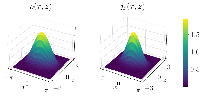
Figure 3: Probability and current densities for the zero-mode written in Eq. (35). Note that the parameters $E_{0}$ and $B_{0}$ modify the amplitude of the curves, whereas the parameters $\mu$ and $\nu$ expand or concentrate the curves for big and small values, respectively. In these plots the scale is set by the parameters $E_{0}=2.0$, $B_{0}=1.0$, $\mu=1.0$ and $\nu=1.0$

As can be seen from Fig. 3, for the zero-mode spinor in Eq. (35), the probability density is almost entirely localized around the origin, whereas the only non-zero current density points in $X$-direction (we do not show the $Y-$ and $Z-$components of the current density as they exactly vanish).

In order to have a better insight of the dynamics, let us look at the chiral decomposition of the spinor. For this purpose, we use the chiral projectors $P_{R,L}=\frac{1}{2}(I\pm\gamma_{5})$, which allow us to obtain the left- (L) and right-handed (R) spinors

$$\Psi_{D;R,L}(t,x,y,z)= e^{i(\varepsilon t+ky)}\Psi_{R,L}(x,z)$$

$$= \frac{1}{2}e^{i(\varepsilon t+ky)}\begin{pmatrix}\psi^{\alpha}_{\uparrow}\pm\psi^{\beta}_{\uparrow}\\ \psi^{\beta}_{\downarrow}\pm\psi^{\alpha}_{\downarrow}\\ \psi^{\beta}_{\uparrow}\pm\psi^{\alpha}_{\uparrow}\\ \psi^{\alpha}_{\downarrow}\pm\psi^{\beta}_{\downarrow}\end{pmatrix},$$ (39)

where the down-sign (up-sign) is chosen for the L(R)-handed spinor. Note that in Eq. (III.1) we are suppressing the $x$- and $z$-dependence of the spinor components to simplify the notation. Chiral projections of the probability density (shown in Fig. 4) are

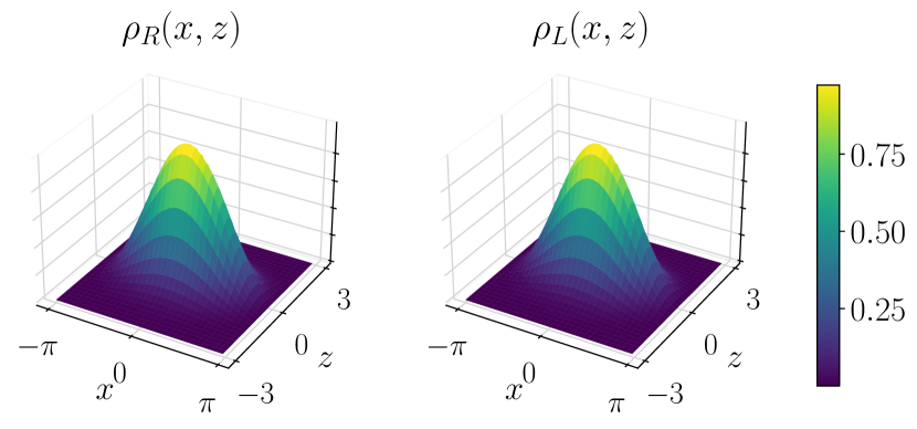
Figure 4: Probability densities for the L- and R-handed spinors in Eq. (III.1), corresponding to the zero-mode spinor in Eq. (35). The scale of the plot is set by the parameters $E_{0}=2.0$, $B_{0}=1.0$, $\mu=1.0$ and $\nu=1.0$.

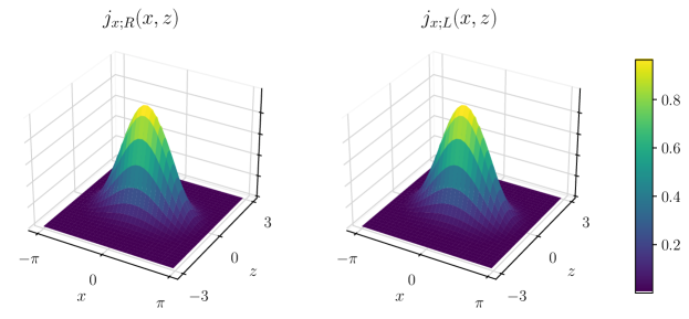
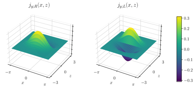
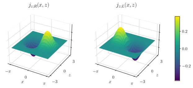
Figure 5: R- and L-chiral probability current densities for the spinors in Eq. (III.1) corresponding to the zero-mode of the system. In $y$- and $z$-directions the R- and L-chiral components are exactly equal but with opposite sign, resulting in null-total current densities. While, in $x$-direction both chiral components contribute to the non-zero current density. The parameter values taken are $E_{0}=2.0$, $B_{0}=1.0$, $\mu=1.0$ and $\nu=1.0$.

$$\rho_{R,L}=\frac{1}{2}\left[|\psi^{\alpha}_{\uparrow}|^{2}+|\psi^{\alpha}_{\downarrow}|^{2}+|\psi^{\beta}_{\uparrow}|^{2}+|\psi^{\beta}_{\downarrow}|^{2}\right]$$

$$\pm\rm{Re}\left[\psi^{*\alpha}_{\phantom{*}\uparrow}\psi^{\beta}_{\uparrow}+\psi^{*\alpha}_{\phantom{*}\downarrow}\psi^{\beta}_{\downarrow}\right],$$ (40)

and of the current densities (see Fig. 5)

$$j_{x;R,L} = \rm{Re}\left[\psi^{*\alpha}_{\phantom{*}\uparrow}\left(\psi^{\alpha}_{\downarrow}\pm\psi^{\beta}_{\downarrow}\right)+\psi^{*\beta}_{\phantom{*}\uparrow}\left(\psi^{\beta}_{\downarrow}\pm\psi^{\alpha}_{\downarrow}\right)\right],$$ (41)

$$j_{y;R,L} = \rm{Im}\left[\psi^{*\alpha}_{\phantom{*}\uparrow}\left(\psi^{\alpha}_{\downarrow}\pm\psi^{\beta}_{\downarrow}\right)+\psi^{*\beta}_{\phantom{*}\uparrow}\left(\psi^{\beta}_{\downarrow}\pm\psi^{\alpha}_{\downarrow}\right)\right],$$ (42)

$$j_{z;R,L} = \rm{Re}\left[\psi^{*\alpha}_{\phantom{*}\uparrow}\psi^{\beta}_{\uparrow}-\psi^{*\alpha}_{\phantom{*}\downarrow}\psi^{\beta}_{\downarrow}\right]$$ (43)

$$\pm \frac{1}{2}\Big{[}|\psi^{\alpha}_{\uparrow}|^{2}+|\psi^{\beta}_{\uparrow}|^{2}-|\psi^{\alpha}_{\downarrow}|^{2}-|\psi^{\beta}_{\downarrow}|^{2}\Big{]}.$$

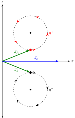
Figure 6: A representation of the right and left chiralities. The sum of the corresponding chiral currents is non-zero in $x$-direction.

A straightforward calculation verifies that the total current densities in Eq. (38) are the sum of the respective L- and R-handed currents, i.e., $j_{i}=j_{i;R}+j_{i;L}$. From Fig. 5, we can observe that the L- and R-handed components of the $y-$ and $z-$current densities cancel out (are opposite), whereas in the $X-$direction, they are exactly the same so that the sum is nonvanishing. From Fig. 4, we note the quantity of particles with L- and R-chiralities is the same (chiral symmetry is conserved). Thus, the continuity equation for the chiral density $\rho_{5}=\rho_{R}-\rho_{L}$ is reduced to

$$\nabla\cdot J_{5}=\frac{1}{2\pi^{2}}E(z)B(x),$$ (44)

where $J_{5}$ is the probability current density associated to $\rho_{5}$ [42, 43]. Taking into account the electromagnetic profiles given in this work, the volume integral of the right-side of Eq. (44) vanishes. Hence, the current density $J_{5}$ describes a circular motion of the chiral particles. It is standard to represent the R-handed chirality ($\eta^{+}$) as a counter-clockwise motion, while L-handed chirality ($\eta^{-}$) is sketched as a clockwise motion. This picture is very useful to gain insight into the behavior of the particles, see Fig. 6, where we can possible observe that the chiral currents sum up in the $X-$direction and cancel out in other directions. In the context of the Dirac materials, given the constrains used to solve the Dirac equation in the previous section, the $X-Z$-plane is the most relevant for the dynamics. Since the non-zero $x$-current density is in the same plane where the electromagnetic fields lie, through our set up we describe a particular case of the Planar Hall Effect (PHE). However, in our case the electromagnetic fields are non-uniform (see Fig. 2), which causes slight differences respect to the standard case where uniform fields are considered [26]. Actually, the inhomogeneous feature of the electromagnetic fields is responsible of the behavior of the particles in the system. Therefore, the current density defining the planar Hall effect is a consequence of the chiral symmetry, which is preserved due to the supersymmetry thereof. We must mention, in the context of Dirac materials, chiral symmetry is translated as the valley symmetry, thus, it is also valid to discuss the dynamics in terms of a valley PHE for the system addressed here.

IV Conclusions

In this article, the (3+1) Dirac equation describing a Dirac material in the presence of static non-uniform parallel electromagnetic fields is solved within a SUSY-QM framework. In order to determine an exact analytic solution, we address the example of electromagnetic profiles leading to Pöschl-Teller-like quantum potentials. The corresponding zero-mode spinor is found and its associated probability and current densities obtained. We notice that the current densities vanish in all spatial directions, except for the current along the $X$-direction, which defines a plane in which it lies perpendicularly to the electromagnetic fields. Hence, it is appropriate to assume that a PHE develops in the system dealt here. Furthermore, since the current densities turn out to be written in terms of the left- and right-handed current densities, the effect can be regarded as driven by the chiral symmetry of the system. A chiral-dependent PHE has been shown in inhomogeneous Weyl semi-metals [42]. However, the Dirac material addressed in this article is pristine but under non-uniform external electromagnetic fields. Therefore, this material shows a new class of chiral PHE. We must mention that the electromagnetic profiles in Eq. (26) are tough to realize in the laboratory. Nevertheless, a configuration of pseudo-electromagnetic fields, associated to strains in the material, could become analogous to the system worked here. Such configuration could be feasible in the laboratory through modern strain techniques in Dirac materials, such as scanning tuneling spectroscopy [44, 45]. Finally, we further remark the localization of the probability density as shown in Fig. 3. In this sense, it is worth noticing that the considered electromagnetic profiles are setting up two Jackiw-Rebbi (J-R) models for the dynamics along in each direction [46, 47, 48]. This observation can be seen precisely in Fig. 1. Thus, the wave packet we are considering in this work should be regarded as a two-dimensional soliton of the J-R type. Therefore, our system could be a promising artificial set up of a wave guide with no energy losses, which could be technologically superb.

References

- [1] Claude Cohen-Tannoudji, Bernard Diu, and Franck Laloë. Quantum mechanics; 1st ed. Wiley, New York, NY, 1977. Trans. of : Mécanique quantique. Paris : Hermann, 1973.
- [2] Jun John Sakurai. Modern quantum mechanics; rev. ed. Addison-Wesley, Reading, MA, 1994.
- [3] David Griffiths. Introduction of Quantum Mechanics. Prentice Hall, Inc., 1995.
- [4] L. Landau. Diamagnetismus der metalle. Zeitschrift für Physik, 64(9):629–637, Sep 1930.
- [5] Vladimir A. Miransky and Igor A. Shovkovy. Quantum field theory in a magnetic field: From quantum chromodynamics to graphene and dirac semimetals. Physics Reports, 576:1–209, 2015. Quantum field theory in a magnetic field: From quantum chromodynamics to graphene and Dirac semimetals.
- [6] Tsuneya Ando, Yukio Matsumoto, and Yasutada Uemura. Theory of hall effect in a two-dimensional electron system. Journal of the Physical Society of Japan, 39(2):279–288, 1975.
- [7] K. v. Klitzing, G. Dorda, and M. Pepper. New method for high-accuracy determination of the fine-structure constant based on quantized hall resistance. Phys. Rev. Lett., 45:494–497, Aug 1980.
- [8] D. C. Tsui, H. L. Stormer, and A. C. Gossard. Two-dimensional magnetotransport in the extreme quantum limit. Phys. Rev. Lett., 48:1559–1562, May 1982.
- [9] R. B. Laughlin. Quantized hall conductivity in two dimensions. Phys. Rev. B, 23:5632–5633, May 1981.
- [10] K. S. Novoselov, A. K. Geim, S. V. Morozov, D. Jiang, M. I. Katsnelson, I. V. Grigorieva, S. V. Dubonos, and A. A. Firsov. Two-dimensional gas of massless dirac fermions in graphene. Nature, 438(7065):197–200, Nov 2005.
- [11] Yuanbo Zhang, Yan-Wen Tan, Horst L. Stormer, and Philip Kim. Experimental observation of the quantum hall effect and berry’s phase in graphene. Nature, 438(7065):201–204, Nov 2005.
- [12] V. P. Gusynin and S. G. Sharapov. Unconventional integer quantum hall effect in graphene. Phys. Rev. Lett., 95:146801, Sep 2005.
- [13] A. K. Geim and K. S. Novoselov. The rise of graphene. Nature Materials, 6(3):183–191, Mar 2007.
- [14] RB Laughlin. The relationship between high-temperature superconductivity and the fractional quantum hall effect. Science, 242(4878):525–533, 1988.
- [15] J. D. Brandenburg, W. Zha, and Z. Xu. Mapping the electromagnetic fields of heavy-ion collisions with the breit-wheeler process. The European Physical Journal A, 57(10):299, Oct 2021.
- [16] Dmitri E. Kharzeev, Larry D. McLerran, and Harmen J. Warringa. The Effects of topological charge change in heavy ion collisions: ’Event by event P and CP violation’. Nucl. Phys. A, 803:227–253, 2008.
- [17] Dmitri E. Kharzeev. The chiral magnetic effect and anomaly-induced transport. Progress in Particle and Nuclear Physics, 75:133–151, 2014.
- [18] Kenji Fukushima, Dmitri E. Kharzeev, and Harmen J. Warringa. Chiral magnetic effect. Phys. Rev. D, 78:074033, Oct 2008.
- [19] Mohamed Abdallah et al. Search for the chiral magnetic effect with isobar collisions at =200 GeV by the STAR Collaboration at the BNL Relativistic Heavy Ion Collider. Phys. Rev. C, 105(1):014901, 2022.
- [20] Volker Koch, Soeren Schlichting, Vladimir Skokov, Paul Sorensen, Jim Thomas, Sergei Voloshin, Gang Wang, and Ho-Ung Yee. Status of the chiral magnetic effect and collisions of isobars. Chin. Phys. C, 41(7):072001, 2017.
- [21] Qiang Li, Dmitri E. Kharzeev, Cheng Zhang, Yuan Huang, I. Pletikosić, A. V. Fedorov, R. D. Zhong, J. A. Schneeloch, G. D. Gu, and T. Valla. Chiral magnetic effect in zrte5. Nature Physics, 12(6):550–554, Jun 2016.
- [22] Cai-Zhen Li, Li-Xian Wang, Haiwen Liu, Jian Wang, Zhi-Min Liao, and Da-Peng Yu. Giant negative magnetoresistance induced by the chiral anomaly in individual cd3as2 nanowires. Nature communications, 6(1):10137, 2015.
- [23] Guolin Zheng, Jianwei Lu, Xiangde Zhu, Wei Ning, Yuyan Han, Hongwei Zhang, Jinglei Zhang, Chuanying Xi, Jiyong Yang, Haifeng Du, Kun Yang, Yuheng Zhang, and Mingliang Tian. Transport evidence for the three-dimensional dirac semimetal phase in . Phys. Rev. B, 93:115414, Mar 2016.
- [24] Xiaochun Huang, Lingxiao Zhao, Yujia Long, Peipei Wang, Dong Chen, Zhanhai Yang, Hui Liang, Mianqi Xue, Hongming Weng, Zhong Fang, Xi Dai, and Genfu Chen. Observation of the chiral-anomaly-induced negative magnetoresistance in 3d weyl semimetal taas. Phys. Rev. X, 5:031023, Aug 2015.
- [25] Shi-Han Zheng, Hou-Jian Duan, Jia-Kun Wang, Jia-Yu Li, Ming-Xun Deng, and Rui-Qiang Wang. Origin of planar hall effect on the surface of topological insulators: Tilt of dirac cone by an in-plane magnetic field. Phys. Rev. B, 101:041408, Jan 2020.
- [26] S. Nandy, Girish Sharma, A. Taraphder, and Sumanta Tewari. Chiral anomaly as the origin of the planar hall effect in weyl semimetals. Phys. Rev. Lett., 119:176804, Oct 2017.
- [27] A. Martín-Ruiz, M. Cambiaso, and L. F. Urrutia. The magnetoelectric coupling in electrodynamics. International Journal of Modern Physics A, 34(28):1941002, 2019.
- [28] E. McCann and M. Koshino. The electronic properties of bilayer graphene. Rep. Prog. Phys., 76:056503, 2013.
- [29] G Margía, A Raya, A Sánchez, and E Reyes. The electron propagator in external electromagnetic fields in lower dimensions. Am. J. Phys, 78:700–707, 2010.
- [30] S. Kuru, J. Negro, and L. M. Nieto. Exact analytic solutions for a dirac electron moving in graphene under magnetic fields. J. Phys.: Condens. Matter, 21:455305, 2009.
- [31] P. Ghosh and P. Roy. Bound states in graphene via fermi velocity modulation. The European Physical Journal Plus, 132(1):32, Jan 2017.
- [32] A. Gangopadhyaya, J. Mallow, and C. Rasinariu. Supersymmetric Quantum Mechanics. World Scientific, Singapore, second edition, 2018.
- [33] G. Junker. Supersymmetric Methods in Quantum, Statistical and Solid State Physics. IOP Publishing Ltd, Bristol, second edition, 2019.
- [34] D. J. Fernández. Trends in supersymmetric quantum mechanics. In Şengül Kuru, Javier Negro, and Luis M. Nieto, editors, Integrability, Supersymmetry and Coherent States: A Volume in Honour of Professor Véronique Hussin, pages 37–68, Cham, 2019. Springer International Publishing.
- [35] Tarun Kanti Ghosh. Exact solutions for a dirac electron in an exponentially decaying magnetic field. Journal of Physics: Condensed Matter, 21(4):045505, dec 2008.
- [36] P Ghosh and P Roy. Dirac equation in (1 + 1) dimensional curved space-time: Bound states and bound states in continuum. Physica Scripta, 96(2):025303, dec 2020.
- [37] David J. Fernández C., Juan D. García M., and Daniel O-Campa. Electron in bilayer graphene with magnetic fields leading to shape invariant potentials. J. Phys. A: Math. Theor., 53(43):435202, oct 2020.
- [38] David J Fernandez, Juan Domingo García, and Daniel Ortiz Campa. Bilayer graphene in magnetic fields generated by supersymmetry. Journal of Physics A: Mathematical and Theoretical, apr 2021.
- [39] David J. Fernández C. and Juan D. García-Muñoz. Graphene in complex magnetic fields. The European Physical Journal Plus, 137(9):1013, Sep 2022.
- [40] Ali Mostafazadeh. Pseudo-hermiticity versus pt symmetry: The necessary condition for the reality of the spectrum of a non-hermitian hamiltonian. Journal of Mathematical Physics, 43(1):205–214, 2002.
- [41] Ali Mostafazadeh. Pseudo-hermiticity versus pt-symmetry. ii. a complete characterization of non-hermitian hamiltonians with a real spectrum. Journal of Mathematical Physics, 43(5):2814–2816, 2002.
- [42] Suvendu Ghosh, Debabrata Sinha, Snehasish Nandy, and A. Taraphder. Chirality-dependent planar hall effect in inhomogeneous weyl semimetals. Phys. Rev. B, 102:121105, Sep 2020.
- [43] Chao-Xing Liu, Peng Ye, and Xiao-Liang Qi. Chiral gauge field and axial anomaly in a weyl semimetal. Phys. Rev. B, 87:235306, Jun 2013.
- [44] N Levy, SA Burke, KL Meaker, M Panlasigui, A Zettl, F Guinea, AH Castro Neto, and Michael F Crommie. Strain-induced pseudo–magnetic fields greater than 300 tesla in graphene nanobubbles. Science, 329(5991):544–547, 2010.
- [45] Nikolai N Klimov, Suyong Jung, Shuze Zhu, Teng Li, C Alan Wright, Santiago D Solares, David B Newell, Nikolai B Zhitenev, and Joseph A Stroscio. Electromechanical properties of graphene drumheads. Science, 336(6088):1557–1561, 2012.
- [46] Roman Jackiw and Cláudio Rebbi. Solitons with fermion number . Physical Review D, 13(12):3398, 1976.
- [47] Alexey A Gorlach, Dmitry V Zhirihin, Alexey P Slobozhanyuk, Alexander B Khanikaev, and Maxim A Gorlach. Photonic jackiw-rebbi states in all-dielectric structures controlled by bianisotropy. Physical Review B, 99(20):205122, 2019.
- [48] Sayan Jana, Arijit Saha, and Sourin Das. Jackiw-rebbi zero modes in non-uniform topological insulator nanowire. Physical Review B, 100(8):085428, 2019.