High-dimensional canonical correlation analysis

Abstract.

This paper studies high-dimensional canonical correlation analysis (CCA) with an emphasis on the vectors that define canonical variables. The paper shows that when two dimensions of data grow to infinity jointly and proportionally, the classical CCA procedure for estimating those vectors fails to deliver a consistent estimate. This provides the first result on the impossibility of identification of canonical variables in the CCA procedure when all dimensions are large. As a countermeasure, the paper derives the magnitude of the estimation error, which can be used in practice to assess the precision of CCA estimates. Applications of the results to cyclical vs. non-cyclical stocks and to a limestone grassland data set are provided.

1. Introduction

1.1. Background

Canonical correlation analysis (CCA) is a classical statistical analysis method used to find a common structure between two data sets. It was first introduced in Hotelling (1936) and remains in active use today. CCA can be viewed as a generalization of principal component analysis (PCA) from one set of variables to two: in PCA the goal is to find a signal (or factor) in a large matrix with a large amount of noise, while CCA searches for a common signal among two large matrices with a large amount of noise. We refer the reader to the textbooks Thompson (1984); Gittins (1985); Anderson (2003), and Muirhead (2009) for introductions to CCA.

There are numerous applications of CCA in the social and natural sciences. In genomics CCA is used to find commonalities between multiple assays coming from the same set of individuals (see, e.g., Witten and Tibshirani (2009) and references therein). In neuroscience it is used to match brain measurements with behavioral and medical scores (e.g., Wang et al. (2020); Zhuang et al. (2020)). Similarly, in ecology CCA is used to correlate characteristics of living species with those of their habitats (e.g., Gittins (1985) and Simon (1998, Chapter 23)). In econometrics CCA is used to select the number of factors driving the behaviour of various processes (see, e.g., Breitung and Pigorsch (2013); Andreou et al. (2019), and Choi et al. (2021)). Further, in time series econometrics CCA appears in cointegration analysis: a strong correlation between first differences (which are stationary) and lags (which are nonstationary) indicates the presence of cointegration (cf. Johansen (1988)).

Beyond the cases outlined above, there are numerous settings where CCA can provide a meaningful alternative approach and complement previous methods. For example, in sociology and applied economics CCA can provide a framework for analysis of the relationships between various measures of socioeconomic characteristics and investments, on one side, and labour market outcomes and associated skills, on the other side (cf. the production function in Cunha et al. (2010) and the results of Papageorge and Thom (2020)). In finance and financial econometrics an important question, which can be addressed via CCA, is whether different types of stocks are highly correlated and, thus, can be used to create portfolios for pairs trading (e.g., one could exploit a correlation between stocks from different industries or between traditional stocks and cryptocurrencies).

One may notice that most of the above examples ideally require working with very large (across all dimensions) data sets. However, the high-dimensional machinery for CCA (in contrast to that for PCA) is still very much underdeveloped. Thus, the development of new tools and theory suitable for high-dimensional settings remains vital. In this paper we aim to provide such techniques.

1.2. High-dimensional CCA setup.

Formally, if we have two random vectors $\mathbf{u}\in\mathbb{R}^{K}$ and $\mathbf{v}\in\mathbb{R}^{M}$, then the first goal of CCA is to find deterministic vectors $\boldsymbol{\alpha}\in\mathbb{R}^{K},\,\boldsymbol{\beta}\in\mathbb{R}^{M}$ that maximize the correlation between $\mathbf{u}^{\mathsf{T}}\boldsymbol{\alpha}$ and $\mathbf{v}^{\mathsf{T}}\boldsymbol{\beta}$, where ^T is the matrix transposition. That is, we are trying to find highly correlated combinations of coordinates of $\mathbf{u}$ and $\mathbf{v}$. The maximal correlation value is called the largest canonical correlation, and the corresponding $\mathbf{u}^{\mathsf{T}}\boldsymbol{\alpha}$ and $\mathbf{v}^{\mathsf{T}}\boldsymbol{\beta}$ form the first pair of canonical variables. Other canonical correlations (there are $\min(K,M)$ of them) can be found iteratively. Equivalently, all canonical correlations can be found as the eigenvalues of $K\times K$ matrix $(\mathbb{E}\mathbf{u}\mathbf{u}^{\mathsf{T}})^{-1}(\mathbb{E}\mathbf{u}\mathbf{v}^{\mathsf{T}})(\mathbb{E}\mathbf{v}\mathbf{v}^{\mathsf{T}})^{-1}(\mathbb{E}\mathbf{v}\mathbf{u}^{\mathsf{T}})$ or as the eigenvalues of the ${M\times M}$ matrix $(\mathbb{E}\mathbf{v}\mathbf{v}^{\mathsf{T}})^{-1}(\mathbb{E}\mathbf{v}\mathbf{u}^{\mathsf{T}})(\mathbb{E}\mathbf{u}\mathbf{u}^{\mathsf{T}})^{-1}(\mathbb{E}\mathbf{u}\mathbf{v}^{\mathsf{T}})$. Multiplying the corresponding eigenvectors of the former and the latter matrices, respectively, by $\mathbf{u}^{\mathsf{T}}$ and $\mathbf{v}^{\mathsf{T}}$, we obtain all the pairs of canonical variables. We call the setup with two random vectors a population formulation.

In contrast, in the sample formulation, two vectors are replaced by two matrices (e.g., we observe $S$ samples of $\mathbf{u}$ and $S$ samples of $\mathbf{v}$). Let those samples be $\mathbf{U}$ ($K\times S$ matrix) and $\mathbf{V}$ ($M\times S$ matrix). The finite sample analogues of the canonical correlations, the sample canonical correlations, are computed by maximizing the sample correlations between the $S$-dimensional vectors $\mathbf{U}^{\mathsf{T}}\widehat{\boldsymbol{\alpha}}$ and $\mathbf{V}^{\mathsf{T}}\widehat{\boldsymbol{\beta}}$. Equivalently, their squares are eigenvalues of $(\mathbf{U}\mathbf{U}^{\mathsf{T}})^{-1}\mathbf{U}\mathbf{V}^{\mathsf{T}}(\mathbf{V}\mathbf{V}^{\mathsf{T}})^{-1}\mathbf{V}\mathbf{U}^{\mathsf{T}}$. The canonical correlation vectors are eigenvectors of the preceding product of matrices and another similar expression. The corresponding $\mathbf{U}^{\mathsf{T}}\widehat{\boldsymbol{\alpha}}$ and $\mathbf{V}^{\mathsf{T}}\widehat{\boldsymbol{\beta}}$ are called sample canonical variables.

Assume that the columns of $\mathbf{U}$ and $\mathbf{V}$ are i.i.d. Then, when $S$ is large while $K$ and $M$ are fixed, the sample covariances of $\mathbf{U}$ and $\mathbf{V}$ as well as their cross-covariances are consistent estimators of their population counterparts. Therefore, $(\mathbf{U}\mathbf{U}^{\mathsf{T}})^{-1}\mathbf{U}\mathbf{V}^{\mathsf{T}}(\mathbf{V}\mathbf{V}^{\mathsf{T}})^{-1}\mathbf{V}\mathbf{U}^{\mathsf{T}}$ is a consistent estimate of its population analogue $(\mathbb{E}\mathbf{u}\mathbf{u}^{\mathsf{T}})^{-1}(\mathbb{E}\mathbf{u}\mathbf{v}^{\mathsf{T}})(\mathbb{E}\mathbf{v}\mathbf{v}^{\mathsf{T}})^{-1}(\mathbb{E}\mathbf{v}\mathbf{u}^{\mathsf{T}})$, and we obtain consistent estimates of the squared correlation coefficients and corresponding vectors. The exact distribution of the sample canonical correlations and variables and their asymptotic behavior in the fixed $K$ and $M$ regime have attracted the attention of many researchers, with the seminal results going back to Hsu (1939, 1941) and Constantine (1963) and the latest corrections to the results on canonical variables being much more recent (see Anderson (1999)).

The properties of CCA when all three dimensions $S,K,M$ are large and comparable have not yet been properly analyzed. The remarkable seminal result in this direction is that of Wachter (1980), who studies the case when $\mathbf{u}$ and $\mathbf{v}$ are uncorrelated and columns $\mathbf{U}$ and $\mathbf{V}$ are independent samples of $\mathbf{u}$ and $\mathbf{v}$, respectively. Wachter (1980) shows that despite $\mathbf{U}$ and $\mathbf{V}$ being independent, the empirical distribution of the sample canonical correlations has a nontrivial limit as $S,K,M\to\infty$ with $S/K\to\tau_{K}$, $S/M\to\tau_{M}$; in particular, the majority of the correlations are bounded away from $0$. The conceptual conclusion is that in the large $S,K,M$ setting the sample canonical correlations do not deliver consistent estimates of the population canonical correlations, which in this case all equal zero due to $\mathbf{u}$ and $\mathbf{v}$ being independent. These results have been extended very recently in Bao et al. (2019) and Yang (2022b) to the case when some (but finitely many as the dimensions grow) population correlations are allowed to be nonzero. Conceptually similar results are obtained: the sample squared canonical correlations are always larger and bounded away from their population counterparts. However, there is an explicit dependence between the sample and population canonical correlations, and therefore, knowing the former allows one to reconstruct the latter. Hence, it is possible to identify nontrivial population canonical correlations.

No progress has been achieved so far to tackle the challenging properties of the corresponding vectors of canonical variables in the regime in which $S,K,M$ are large and proportional to each other. In practice squared correlation coefficients can be used to test whether there is a common signal between two data sets (i.e., the largest coefficient is statistically larger than zero). However, vectors are required to be able to say something about the nature of this commonality: where it comes from, what it represents, etc. The asymptotic analysis of these vectors is the central topic of the present paper.

To address the problem of estimating CCA vectors, we first assume that $\mathbf{U}$ and $\mathbf{V}$ are Gaussian and independent across $S$ samples of $\mathbf{u}$ and $\mathbf{v}$ but allow $\mathbf{u}$ to be correlated with $\mathbf{v}$. We start with $\mathbf{u}$ and $\mathbf{v}$ having exactly one nonzero canonical correlation and refer to it as the signal, while the remaining uncorrelated parts of $\mathbf{u}$ and $\mathbf{v}$ are viewed as the noise. We characterize (in terms of the parameters $S,K,M$ and the covariances between coordinates of $\mathbf{u}$ and $\mathbf{v}$) when we can detect a nonzero canonical correlation, i.e., when there is enough signal in the data compared to the pure noise case. Next, we develop formulas for sample $\widehat{\boldsymbol{\alpha}}$ and $\widehat{\boldsymbol{\beta}}$, which allow us to show that, for finite ratios $S/K,\,S/M$, one cannot consistently estimate true values $\boldsymbol{\alpha}$ and $\boldsymbol{\beta}$. The estimated canonical variables $\mathbf{U}^{\mathsf{T}}\widehat{\boldsymbol{\alpha}}$ and $\mathbf{V}^{\mathsf{T}}\widehat{\boldsymbol{\beta}}$ will always lie on cones around the true population canonical variables $\mathbf{U}^{\mathsf{T}}\boldsymbol{\alpha}$ and $\mathbf{V}^{\mathsf{T}}\boldsymbol{\beta}$. We provide explicit formulas for the width of these cones. They show that the cones shrink as we increase the ratios $S/K,\,S/M$ and that ultimately consistency is restored in the limit.

Next, we provide various generalizations from the i.i.d. Gaussian setting with one signal. First, motivated by the fact that often data are far from normal (especially in financial applications), we relax our assumptions to accommodate any distribution as long as its first four moments match the Gaussian moments. Second, we allow for correlated realizations. We do this separately for signal parts (i.e., the signal is not independent across $S$) and for the noise part (i.e., the noise is not independent across $S$). Finally, we extend the machinery to allow for multiple vectors $\boldsymbol{\alpha}$ and $\boldsymbol{\beta}$, i.e., multiple nonzero canonical correlations in the population setting. In other words, we allow the signal to be of any finite rank, and the vectors $\boldsymbol{\alpha}$ and $\boldsymbol{\beta}$ are replaced by matrices.

1.3. Other related literature

CCA is closely connected to the literature on factors. First, as mentioned above, some methods for factor estimation rely on CCA. The idea is that the correlation between different sets of variables, which is captured by CCA, can be fundamentally related to the presence and properties of factors. For instance, one can distinguish between common and group-specific factors (see, e.g., Andreou et al. (2019) and Choi et al. (2021)).

Another point of view on the interconnection between factors and CCA comes from the interpretation of canonical variables as common explanatory factors between two data sets. The main difference is that factors operate with a single matrix/data set while canonical correlations require two matrices/data sets. The main approach for finding factors is via PCA and its modifications (cf. Bai and Ng (2008); Stock and Watson (2011); Fan et al. (2016) and references therein). There are many similarities in the spirit of the modeling and results between CCA and PCA. However, CCA as considered in our present paper is much more challenging and involved than PCA. This is perhaps an inherent feature of the CCA procedure, which involves matrix inversion, a much more complicated operation to carry out than simply calculating a product.

In statistics and probability factors (signals in the data) are often modeled as a spiked random matrix. A spiked random matrix is a sum of a full-rank noise matrix and a small-rank signal matrix. Often this is embedded in the PCA setting: one observes a matrix $C=A+B$, where $A$ is treated as a low-rank signal and $B$ is treated as noise, and tries to reconstruct $A$ from observing $C$ through its singular values and vectors. $A$, $B$, and $C$ here are rectangular matrices with both dimensions assumed to be large. In econometrics $A$ represents a product of factors and their loadings, while $B$ is composed of idiosyncratic errors.

For such a setting, Baik et al. (2005) and Baik and Silverstein (2006) discovered the phenomenon now known as the BBP phase transition: when the signal is small while the noise is given by a matrix with i.i.d. mean zero elements, one cannot detect the presence of the signal from singular values of $C$, while for a large signal, the largest singular values of $C$ connect to those of $A$ through explicit formulas. The corresponding singular vectors can be used as an estimate of $A$; however, this estimate is inconsistent, in parallel to what we observe in the CCA setting (see Johnstone and Lu (2009); Paul (2007); Nadler (2008) and references therein for earlier work in the learning theory literature in physics). If we extend the parallel, consistency in the PCA setting can be partially restored if we allow one of the dimensions of the rectangular matrix of interest to be much larger than another. In the econometrics literature, the same transition appears in the framework of weakly influential factors (see Onatski (2012) and references therein); when factors become strong, estimation consistency is restored.

Even closer to our setting is that in Gavish et al. (2022), which deals with spiked $F$–matrices (and also contains many other references). An $F$–matrix, which comes from the $F$–test, deals with the ratio of two large matrices. In the benchmark situation of no spikes (or no signal) there is a way to directly match an $F$–matrix with random matrices appearing in CCA. However, this connection disappears as soon as signals in the data are present.

1.4. Outline of the paper.

The remainder of the paper is organised as follows. Section 2 discusses the basic setting of i.i.d. normal vectors. Various generalizations (to the cases with nonnormal errors, correlated observations, and multiple signals) are presented in Section 3. Section 4 provides two empirical illustrations of our results. Finally, Section 5 concludes. Proofs and additional data details are given in appendices.

2. Basic framework

2.1. Population setting

Let $\mathbf{u}=(u_{1},\dots,u_{K})^{\mathsf{T}}$ and $\mathbf{v}=(v_{1},\dots,v_{M})^{\mathsf{T}}$ be $K$- and $M$- dimensional random vectors with zero means and nondegenerate covariance matrices, where $\,{}^{\mathsf{T}}$ here and below denotes matrix transposition. Without loss of generality, we assume $K\leq M$.

Assumption I.

The vectors $\mathbf{u}$ and $\mathbf{v}$ satisfy the following:

1. The vectors $\mathbf{u}$ and $\mathbf{v}$ are jointly Gaussian with zero means.

2. There exist nonzero deterministic vectors $\boldsymbol{\alpha}\in\mathbb{R}^{K},\,\boldsymbol{\beta}\in\mathbb{R}^{M}$ such that

   1. For any $\boldsymbol{\gamma}\in\mathbb{R}^{K}$, if $\mathbf{u}^{\mathsf{T}}\boldsymbol{\alpha}$ and $\mathbf{u}^{\mathsf{T}}\boldsymbol{\gamma}$ are uncorrelated, then $\mathbf{v}$ and $\mathbf{u}^{\mathsf{T}}\boldsymbol{\gamma}$ are also uncorrelated;

   2. For any $\boldsymbol{\gamma}\in\mathbb{R}^{M}$, if $\mathbf{v}^{\mathsf{T}}\boldsymbol{\beta}$ and $\mathbf{v}^{\mathsf{T}}\boldsymbol{\gamma}$ are uncorrelated, then $\mathbf{u}$ and $\mathbf{v}^{\mathsf{T}}\boldsymbol{\gamma}$ are also uncorrelated.

The pair $(\mathbf{u}^{\mathsf{T}}\boldsymbol{\alpha},\mathbf{v}^{\mathsf{T}}\boldsymbol{\beta})$ represents the signal in the data, while the remaining part is treated as the noise, which is uncorrelated with the signal. Ultimately, we are interested in the signal and would like to filter out the influence of the noise.

Example 2.1.

Assumption I is satisfied with $\boldsymbol{\alpha}=(1,0,\ldots,0)^{\mathsf{T}},\,\boldsymbol{\beta}=(1,0,\ldots,0)^{\mathsf{T}}$ if $(u_{1},\dots,u_{K},v_{1},\dots,v_{M})^{\mathsf{T}}$ is a mean zero Gaussian vector such that, for each $2\leq k\leq K$, the coordinate $u_{k}$ is uncorrelated with $u_{1}$ and with $v_{1},\dots,v_{M}$ and, for each $2\leq m\leq M$, the coordinate $v_{m}$ is uncorrelated with $v_{1}$ and with $u_{1},\dots,u_{K}$. In other words, the only possible nonzero correlations are between $u_{1}$ and $v_{1}$, between $u_{k}$ and $u_{k^{\prime}}$, $2\leq k,k^{\prime}\leq K$, and between $v_{m}$ and $v_{m^{\prime}}$, $2\leq m,m^{\prime}\leq M$. These correlations can be arbitrary.

Any other example can be obtained from the preceding by a change of basis.

Definition 2.2.

Let $C_{uu}:=\mathbb{E}(\mathbf{u}^{\mathsf{T}}\boldsymbol{\alpha})^{2}$, $C_{vv}:=\mathbb{E}(\mathbf{v}^{\mathsf{T}}\boldsymbol{\beta})^{2}$, $C_{uv}=C_{vu}:=\mathbb{E}(\mathbf{u}^{\mathsf{T}}\boldsymbol{\alpha})(\mathbf{v}^{\mathsf{T}}\boldsymbol{\beta})$ and $r^{2}$ be the squared correlation coefficient:

$$r^{2}:=\frac{C_{uv}^{2}}{C_{uu}C_{vv}}.$$

The number $r^{2}$ and the vectors $\boldsymbol{\alpha}$ and $\boldsymbol{\beta}$ of Assumption I can be read from the covariance structure of $\mathbf{u}$ and $\mathbf{v}$, as the following lemma explains.

Lemma 2.3.

The number $r^{2}$ equals the single nonzero eigenvalue of the $K\times K$ matrix $(\mathbb{E}\mathbf{u}\mathbf{u}^{\mathsf{T}})^{-1}(\mathbb{E}\mathbf{u}\mathbf{v}^{\mathsf{T}})(\mathbb{E}\mathbf{v}\mathbf{v}^{\mathsf{T}})^{-1}(\mathbb{E}\mathbf{v}\mathbf{u}^{\mathsf{T}})$ and the single nonzero eigenvalue of the ${M\times M}$ matrix $(\mathbb{E}\mathbf{v}\mathbf{v}^{\mathsf{T}})^{-1}(\mathbb{E}\mathbf{v}\mathbf{u}^{\mathsf{T}})(\mathbb{E}\mathbf{u}\mathbf{u}^{\mathsf{T}})^{-1}(\mathbb{E}\mathbf{u}\mathbf{v}^{\mathsf{T}})$. $\boldsymbol{\alpha}$ and $\boldsymbol{\beta}$ are the corresponding eigenvectors of the former and the latter matrices, respectively.

2.2. Sample setting

Let $\mathbf{W}=\begin{pmatrix}\mathbf{U}\\ \mathbf{V}\end{pmatrix}$ be a $(K+M)\times S$ matrix composed of $S$ independent samples of $\begin{pmatrix}\mathbf{u}\\ \mathbf{v}\end{pmatrix}$. The matrix $\mathbf{W}$ represents observed data, which comes from the population setting 2.1. We are interested in finding the signal $(\mathbf{u}^{\mathsf{T}}\boldsymbol{\alpha},\mathbf{v}^{\mathsf{T}}\boldsymbol{\beta})$ or vectors $(\boldsymbol{\alpha},\boldsymbol{\beta})$. In the sample setting they come from the squared sample canonical correlations and their corresponding vectors. The vectors for the largest correlation represent the sample analogues of $\boldsymbol{\alpha}$ and $\boldsymbol{\beta}$. The following definition is motivated as a sample version of Lemma 2.3.

Definition 2.4.

The squared sample canonical correlations $\lambda_{1}\geq\lambda_{2}\geq\dots\geq\lambda_{K}$ are defined as eigenvalues of the $K\times K$ matrix $(\mathbf{U}\mathbf{U}^{\mathsf{T}})^{-1}\mathbf{U}\mathbf{V}^{\mathsf{T}}(\mathbf{V}\mathbf{V}^{\mathsf{T}})^{-1}\mathbf{V}\mathbf{U}^{\mathsf{T}}$ or as the $K$ largest eigenvalues of the $M\times M$ matrix $(\mathbf{V}\mathbf{V}^{\mathsf{T}})^{-1}\mathbf{V}\mathbf{U}^{\mathsf{T}}(\mathbf{U}\mathbf{U}^{\mathsf{T}})^{-1}\mathbf{U}\mathbf{V}^{\mathsf{T}}$. We set $\widehat{\boldsymbol{\alpha}}$ to be the eigenvector of the former matrix, corresponding to its largest eigenvalue, and we set $\widehat{\boldsymbol{\beta}}$ to be the eigenvector of the latter matrix, corresponding to its largest eigenvalue.

The sample canonical variables are defined as $\widehat{\mathbf{x}}=\mathbf{U}^{\mathsf{T}}\widehat{\boldsymbol{\alpha}}$ and $\widehat{\mathbf{y}}=\mathbf{V}^{\mathsf{T}}\widehat{\boldsymbol{\beta}}$. We also set $\mathbf{x}=\mathbf{U}^{\mathsf{T}}\boldsymbol{\alpha}$ and $\mathbf{y}=\mathbf{V}^{\mathsf{T}}\boldsymbol{\beta}$.

2.3. Results

In the sample setting of Section 2.2, we are going to assume that $S/K\to\tau_{K}$, $S/M\to\tau_{M}$, and $r^{2}\to\rho^{2}$. We define five constants depending on these parameters:

(1) $$\lambda_{\pm} =\left(\sqrt{\tau_{M}^{-1}(1-\tau_{K}^{-1})}\pm\sqrt{\tau_{K}^{-1}(1-\tau_{M}^{-1})}\right)^{2},$$

(2) $$z_{\rho} =\frac{\bigl{(}(\tau_{K}-1)\rho^{2}+1\bigr{)}\bigl{(}(\tau_{M}-1)\rho^{2}+1\bigr{)}}{\rho^{2}\tau_{K}\tau_{M}},$$

(3) $$\mathfrak{s}_{x} =\frac{(1-\rho^{2})(\tau_{K}-1)}{(\tau_{M}-1)(\tau_{K}-1)\rho^{2}-1}\cdot\frac{(\tau_{M}-1)\rho^{2}+1}{(\tau_{K}-1)\rho^{2}+1},$$

(4) $$\mathfrak{s}_{y} =\frac{(1-\rho^{2})(\tau_{M}-1)}{(\tau_{M}-1)(\tau_{K}-1)\rho^{2}-1}\cdot\frac{(\tau_{K}-1)\rho^{2}+1}{(\tau_{M}-1)\rho^{2}+1}.$$

Theorem 2.5.

Suppose that Assumption I holds, that the columns of the data matrix $\mathbf{W}$ are i.i.d., and that the squared sample canonical correlations and variables are constructed as in Section 2.2. Let $S$ tend to infinity and $K\leq M$ depend on it in such a way that the ratios $S/K$ and $S/M$ converge to $\tau_{K}>1$ and $\tau_{M}>1$, respectively, and $\tau_{M}^{-1}+\tau_{K}^{-1}<1$. Simultaneously, suppose that $\lim_{S\to\infty}r^{2}=\rho^{2}$.

1. If $\rho^{2}>\tfrac{1}{\sqrt{(\tau_{M}-1)(\tau_{K}-1)}}$, then $z_{\rho}>\lambda_{+}$, and for the two largest squared sample canonical correlations ${\lambda_{1}\geq\lambda_{2}}$, we have

   (5) $$\lim_{S\to\infty}\lambda_{1}=z_{\rho},\qquad\lim_{S\to\infty}\lambda_{2}=\lambda_{+}\qquad\text{in probability}.$$

   The squared sine of the angle $\theta_{x}$ between $\mathbf{x}$ and $\widehat{\mathbf{x}}$ defined as $\sin^{2}\theta_{x}=1-\frac{(\mathbf{x}^{\mathsf{T}}\widehat{\mathbf{x}})^{2}}{(\mathbf{x}^{\mathsf{T}}\mathbf{x})(\widehat{\mathbf{x}}^{\mathsf{T}}\widehat{\mathbf{x}})}$ satisfies

   (6) $$\lim_{S\to\infty}\sin^{2}\theta_{x}=\mathfrak{s}_{x}\qquad\text{in probability}.$$

   The squared sine of the angle $\theta_{y}$ between $\mathbf{y}$ and $\widehat{\mathbf{y}}$ satisfies

   (7) $$\lim_{S\to\infty}\sin^{2}\theta_{y}=\mathfrak{s}_{y}\qquad\text{in probability}.$$

2. If instead $\rho^{2}\leq\tfrac{1}{\sqrt{(\tau_{M}-1)(\tau_{K}-1)}}$, then

   (8) $$\lim_{S\to\infty}\lambda_{1}=\lambda_{+}\qquad\text{in probability}.$$

Remark 2.6.

While we do not prove it in this text, we expect (based on the related results in Benaych-Georges and Nadakuditi (2011, 2012) and Bloemendal et al. (2016)) that in the case $\bf 2$ with strict inequality the angles $\theta_{x}$ and $\theta_{y}$ tend to $\pi/2$ as $S\to\infty$, with distance to $\pi/2$ of order $S^{-1/2}$ (see Figure 2 for an illustration). Intuitively, it suggests that there is no way to recover asymptotic information on $\boldsymbol{\alpha}$ or $\boldsymbol{\beta}$ in this case.

In the critical case when $\rho^{2}$ is close to $\tfrac{1}{\sqrt{(\tau_{M}-1)(\tau_{K}-1)}}$, we expect that the angles $\theta_{x}$ and $\theta_{y}$ still tend to $\pi/2$, but the convergence might be very slow: a comparison with Bloemendal et al. (2016) and Bao and Wang (2022) predicts the distance to $\pi/2$ to be of order $S^{-1/6}$.

Figure 1 illustrates the dependence of $\mathfrak{s}_{x},\mathfrak{s}_{y},z_{\rho}$ on the squared correlation coefficient $\rho^{2}$. Notice that $z_{\rho}$ as a function of $\rho^{2}$ has a minimum at the cutoff $\rho^{2}=\tfrac{1}{\sqrt{(\tau_{M}-1)(\tau_{K}-1)}}$ and is monotone increasing above the cutoff. The values of $s_{\mathbf{x}}$ and $s_{\mathbf{y}}$ are between $0$ and $1$ for $\rho^{2}$ above the same cutoff. These properties continue to hold for general values of $\tau_{K},\tau_{M}>1$.

Figure 2 shows results from a single simulation (for each fixed value $\rho^{2}$, we run one simulation) vs. theoretical predictions. As we can see, the simulated path is very close to the theoretical one, with largest discrepancy around the cutoff $\tfrac{1}{\sqrt{(\tau_{M}-1)(\tau_{K}-1)}}$.

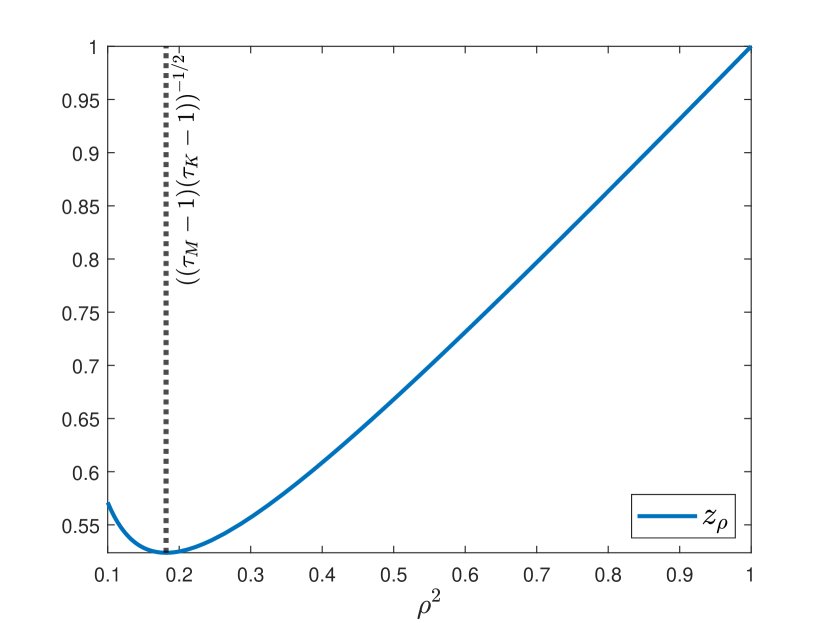
(a) $z_{\rho}$ as a function of $\rho^{2}$.

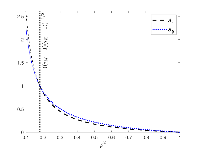
(b) $\mathfrak{s}_{x}$ and $\mathfrak{s}_{y}$ as functions of $\rho^{2}$.

Figure 1. Illustration of Eq. (2), (3), (4) for $K=1000,\,M=1500,\,S=8000$.

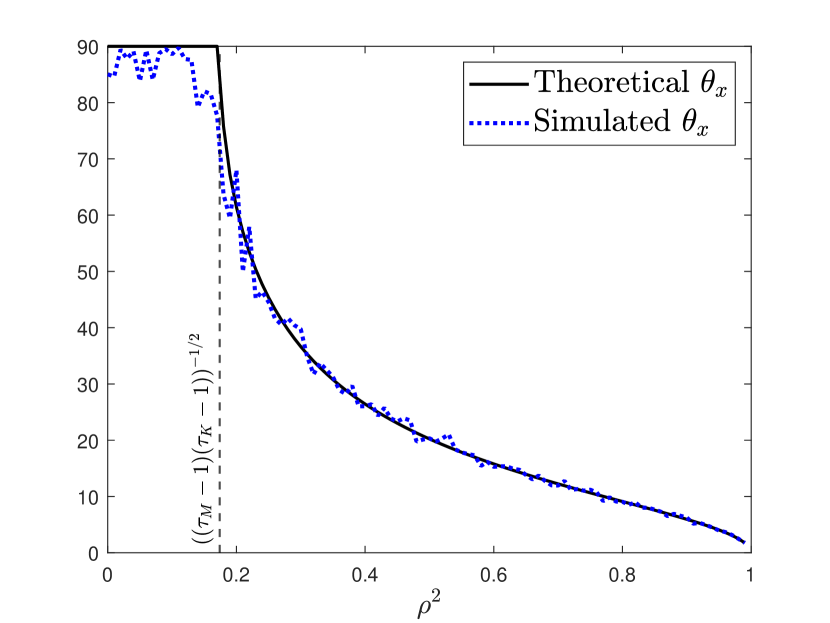
(a) Values of $\theta_{x}$ (in degrees):
theoretical and simulated angles.

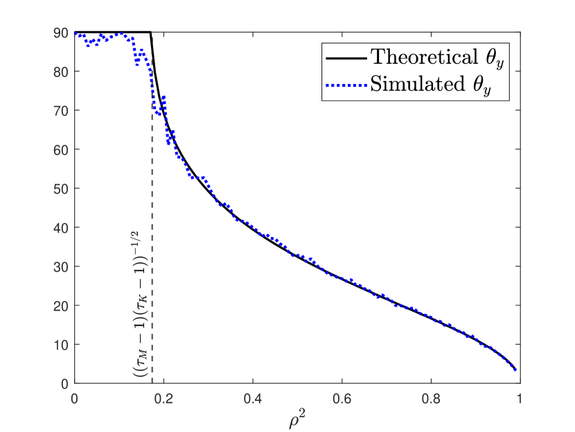
(b) Values of $\theta_{y}$ (in degrees):
theoretical and simulated angles.

Figure 2. Comparison of theoretical and simulated results for ${K=500}$, ${M=2500}$, $S=8000$. Simulated curves are based on one simulation from a fixed value $\rho^{2}$.

2.4. Implications of Theorem 2.5

There are several aspects of Theorem 2.5 worth emphasizing. First, in practice, when one is working with real data, the true value of $\rho$ is unknown, and the results of Theorem 2.5 should be applied in the following way.

Given that the model matches the data, by Wachter (1980) and Johnstone (2008), most of the squared canonical correlations should belong to the $[\lambda_{-},\lambda_{+}]$ interval. If there is a gap between the largest canonical correlation $\lambda_{1}$ and $\lambda_{+}$, as in Figure 3, then in line with Eq. (5), one can take $\lambda_{1}$ as an approximation of $z_{\rho}$. Treating $z_{\rho}$ as known and approximating $\tau_{K}$, $\tau_{M}$ with $S/K$, $S/M$, Eq. (2) becomes a quadratic equation in $\rho^{2}$. Solving it (using $\tfrac{1}{\sqrt{(\tau_{M}-1)(\tau_{K}-1)}}\leq\rho^{2}\leq 1$ to choose the correct root out of the two), we obtain an estimate for $\rho^{2}$, and further plugging into (3) and (4) and using (6) and (7), we obtain an estimate for the angle between $\mathbf{x}$ and $\widehat{\mathbf{x}}$ or between $\mathbf{y}$ and $\widehat{\mathbf{y}}$. If several canonical correlations larger than $\lambda_{+}$ are observed, then one needs to use an extension of Theorem 2.5 provided in Theorem 3.7: for each of these canonical correlations one can use exactly the same procedure as just outlined.

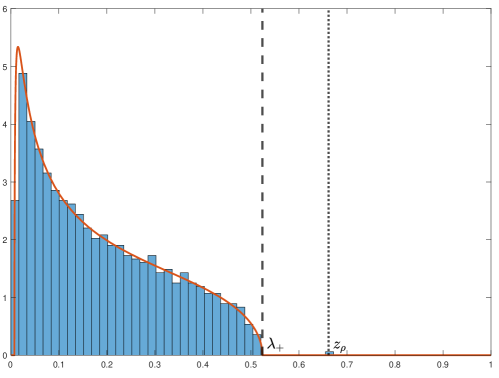
Figure 3. Illustration of Theorem 2.5 with $K=1000$, $M=1500$, $S=8000$, $r^{2}=0.49$. We observe a single spike in the squared sample canonical correlations approximately at $z_{\rho}$ location. The density of the Wachter distribution with corresponding parameters is shown in orange.

The second essential aspect of Theorem 2.5 is the choice of the angles $\theta_{x}$ (between $\widehat{\mathbf{x}}$ and $\mathbf{x}$) and $\theta_{y}$ (between $\widehat{\mathbf{y}}$ and $\mathbf{y}$) as the measure of the quality of approximations of $\widehat{\boldsymbol{\alpha}}$ and $\widehat{\boldsymbol{\beta}}$ for $\boldsymbol{\alpha}$ and $\boldsymbol{\beta}$, respectively. In principle, one could have concentrated on the angle between $\widehat{\boldsymbol{\alpha}}$ and $\boldsymbol{\alpha}$ (or $\widehat{\boldsymbol{\beta}}$ and $\boldsymbol{\beta}$) instead. However, those angles depend on the choice of units of measurement: the angle changes if we multiply one of the coordinates of $\boldsymbol{\alpha}$ by a constant (equivalently, divide a component of $\mathbf{u}$ or a row in $\mathbf{U}$ by the same constant). Hence, asymptotic theory for these angles would require some normalization conditions on the coordinates of $\mathbf{u}$ (and, in fact, correlations between different components of $\mathbf{u}$ would also become important), but such natural normalizations are rare in real data because different coordinates of $\mathbf{u}$ might be coming from very different sources or types of observations. By concentrating on $\theta_{x}$ and $\theta_{y}$, we avoid this problem entirely, and in particular, the result in Theorem 2.5 does not depend on the covariance matrix of the vector $\mathbf{u}$ (and similarly on the covariance matrix of the vector $\mathbf{v}$), which can be arbitrary, as long as it satisfies Assumption I.

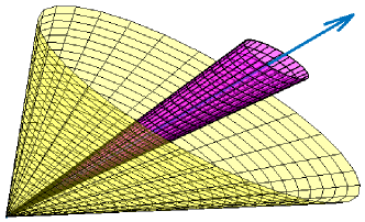
Figure 4. The estimated canonical variable belongs to a cone whose axis is the true direction shown by the blue arrow. If $\sin^{2}\theta$ is small, then the cone is narrow, as shown in purple; if $\sin^{2}\theta$ is large, then the cone is wide, as shown in yellow.

Finally, the angles $\theta_{x}$, $\theta_{y}$ and the limiting value $z_{\rho}$ for the largest squared canonical correlation depend on $\rho$, $\tau_{K}$, and $\tau_{M}$ in a nontrivial fashion, leading to important features of the formulas (2), (3), and (4):

• For any values of $\tau_{K}>1$, $\tau_{M}>1$ with $\tau_{K}^{-1}+\tau_{M}^{-1}<1$ and $\tfrac{1}{\sqrt{(\tau_{M}-1)(\tau_{K}-1)}}<\rho^{2}<1$, we always have $z_{\rho}>\rho^{2}$ and $\mathfrak{s}_{x}>0$, $\mathfrak{s}_{y}>0$ (see Figure 1). In other words, the largest sample canonical correlation overestimates the true largest correlation $\rho^{2}$, while the estimates for the canonical variables are never consistent but rather inclined by nonvanishing angles toward the desired true directions (see Figure 4).

• If $\tau_{K}>1$, $\tau_{M}>1$ with $\tau_{K}^{-1}+\tau_{L}^{-1}<1$ and $\rho^{2}<\tfrac{1}{\sqrt{(\tau_{M}-1)(\tau_{K}-1)}}$, then the asymptotic value of the largest canonical correlation, $\lambda_{+}$, is again larger than $\rho^{2}$. While we do not prove it in this text, we expect that the asymptotic values of $\sin^{2}\theta_{x}$ and $\sin^{2}\theta_{y}$ are close to $1$ in this situation, i.e., that the estimates for the canonical variables are almost orthogonal to the desired true directions (cf. the simulated curves in Figure 2).

• If both $\tau_{K}$ and $\tau_{M}$ become large while $\rho^{2}$ is fixed, then the condition $\rho^{2}>\tfrac{1}{\sqrt{(\tau_{M}-1)(\tau_{K}-1)}}$ becomes trivially true, $z_{\rho}\to\rho^{2}$ and $\mathfrak{s}_{x},\mathfrak{s}_{y}\to 0$. Therefore, $z_{\rho}$, $\widehat{\mathbf{x}}$, and $\widehat{\mathbf{y}}$ become consistent estimates of $\rho^{2}$, $\mathbf{x}$ and $\mathbf{y}$, respectively.

• If $\tau_{K}$ becomes large while $\rho^{2}$ and $\tau_{M}$ remain fixed (this means that $M$ and $S$ are of the same magnitude but $K$ is much smaller), then $z_{\rho}$ remains larger than $\rho^{2}$, and $\mathfrak{s}_{y}$ remains positive. However, $\mathfrak{s}_{x}$ tends to $0$, which means that $\widehat{\mathbf{x}}$ becomes a consistent estimate of $\mathbf{x}$.

3. General framework

In the previous section we presented our main theorem in the basic setting of i.i.d. Gaussian data with a single nonzero canonical correlation in the population. The results are the most transparent in this case, yet many important generalizations can be derived. In this section we state four such generalizations by

1. Relaxing Gaussianity Assumption I.(1);

2. Allowing for signals $\mathbf{u}^{\mathsf{T}}\boldsymbol{\alpha}$ and $\mathbf{v}^{\mathsf{T}}\boldsymbol{\beta}$ that are correlated along dimension $S$;

3. Allowing for noise (orthogonal to $\mathbf{u}^{\mathsf{T}}\boldsymbol{\alpha}$ and $\mathbf{v}^{\mathsf{T}}\boldsymbol{\beta}$) that is correlated along dimension $S$ at the expense of more complicated formulas governing the answers in an extension of Theorem 2.5; and

4. Allowing for multiple signals.

3.1. Non-Gaussian data

Definition 3.1.

We say that a mean zero random vector $(X_{1},\dots,X_{n})$ is fourth-moment Gaussian if there exists a jointly Gaussian mean zero vector $(Y_{1},\dots,Y_{n})$ such that the covariance matrix and the joint fourth moments of $(X_{i})_{i=1}^{n}$ match those of $(Y_{i})_{i=1}^{n}$.

Definition 3.1 is equivalent to requiring the fourth joint moments of $(X_{1},\dots,X_{n})$ to satisfy the Wick rule: for any $1\leq i,j,k,l\leq n$, we should have

(9) $$\mathbb{E}X_{i}X_{j}X_{k}X_{l}=\mathbb{E}X_{i}X_{j}\cdot\mathbb{E}X_{k}X_{l}+\mathbb{E}X_{i}X_{k}\cdot\mathbb{E}X_{j}X_{l}+\mathbb{E}X_{i}X_{l}\cdot\mathbb{E}X_{j}X_{k}.$$

For $n=1$, (9) reduces to a single condition $\mathbb{E}X_{1}^{4}=3[\mathbb{E}X_{1}^{2}]^{2}$. For $n=2$, there are five conditions: $\mathbb{E}X_{1}^{4}=3[\mathbb{E}X_{1}^{2}]^{2}$, $\mathbb{E}X_{1}^{3}X_{2}=3\mathbb{E}X_{1}^{2}\mathbb{E}X_{1}X_{2}$, $\mathbb{E}X_{1}^{2}X_{2}^{2}=\mathbb{E}X_{1}^{2}\mathbb{E}X_{2}^{2}+2[\mathbb{E}X_{1}X_{2}]^{2}$, $\mathbb{E}X_{1}X_{2}^{3}=3\mathbb{E}X_{1}X_{2}\mathbb{E}X_{2}^{2}$, and $\mathbb{E}X_{2}^{4}=3[\mathbb{E}X_{2}^{2}]^{2}$.

We now present a relaxation of Assumption I on the random vectors $\mathbf{u}\in\mathbb{R}^{K}$ and $\mathbf{v}\in\mathbb{R}^{M}$.

Assumption II.

There exists a deterministic vector $\boldsymbol{\alpha}\in\mathbb{R}^{K}$ and a deterministic $(K-1)\times K$ matrix $A$ of rank $K-1$; and a deterministic vector $\boldsymbol{\beta}\in\mathbb{R}^{M}$ and a deterministic $(M-1)\times M$ matrix $B$ of rank $M-1$ such that

1. The random variables $\mathbf{u}^{\mathsf{T}}\boldsymbol{\alpha}$ and $\mathbf{v}^{\mathsf{T}}\boldsymbol{\beta}$ are jointly fourth-moment Gaussian with mean zero, as in Definition 3.1 with $n=2$.

2. There exists a $(K+M-2)$–dimensional vector $(\tilde{\mathbf{u}}^{\mathsf{T}},\tilde{\mathbf{v}}^{\mathsf{T}})^{\mathsf{T}}$ where $\tilde{\mathbf{u}}$ has coordinates $(\tilde{u}_{i})_{i=1}^{K-1}$ and $\tilde{\mathbf{v}}$ has coordinates $(\tilde{v}_{j})_{j=1}^{M-1}$, for which

   • All components $\tilde{u}_{1},\dots,\tilde{u}_{K-1},\tilde{v}_{1},\dots,\tilde{v}_{M-1}$ are jointly independent with each other and with both $\mathbf{u}^{\mathsf{T}}\boldsymbol{\alpha}$ and $\mathbf{v}^{\mathsf{T}}\boldsymbol{\beta}$.

   • $\mathbb{E}\tilde{u}_{i}=0$, $\mathbb{E}\tilde{u}_{i}^{2}=1$, $1\leq i<K$, and $\mathbb{E}\tilde{v}_{j}=0$, $\mathbb{E}\tilde{v}_{j}^{2}=1$, $1\leq j<M$.

   • For constants $\kappa>0$ and $C>0$, $\sup_{i}\mathbb{E}|\tilde{u}_{i}|^{4+\kappa}<C$ and $\sup_{j}\mathbb{E}|\tilde{v}_{j}|^{4+\kappa}<C$.

   • $A\mathbf{u}=\tilde{\mathbf{u}}$ and $B\mathbf{v}=\tilde{\mathbf{v}}$.

Assumption II splits the vectors $\mathbf{u}$ and $\mathbf{v}$ into two components: the correlated signal part $(\mathbf{u}^{\mathsf{T}}\boldsymbol{\alpha},\mathbf{v}^{\mathsf{T}}\boldsymbol{\beta})$ and the remaining noise part $(A\mathbf{u},B\mathbf{v})$. The coordinates of the latter are independent but not necessarily identically distributed. Assumptions I and II coincide in the case of Gaussian $\mathbf{u}$ and $\mathbf{v}$.

Theorem 3.2.

If we replace Assumption I with Assumption II, then Theorem 2.5 continues to hold with exactly the same conclusion.

(a) CCA eigenvalues and Wachter distribution.

Angles (in degrees)
	Theoretical	Simulation
$\theta_{x}$	$25.22$	$25.40$
$\theta_{y}$	$28.39$	$29.60$

(b) Theoretical angles and corresponding angles from one simulation with one signal and $U[-1,1]$ errors.

Figure 5. Illustration for the results with one signal and $U[-1,1]$ errors, ${K=1000}$, $M=1500$, $S=8000$, $r^{2}=0.49$.

The implications of Theorem 3.2 are the same as those discussed in Section 2.4. Thus, practical implementations remain the same. One can possibly relax or come up with alternatives to our moment conditions in Assumption II (see Yang (2022b) for one possible approach). As shown in Figure 5, uniform errors $U[-1,1]$, whose fourth moment does not coincide with the fourth moment of a Gaussian distribution, still lead to the same results as in Theorem 3.2.

3.2. Correlated signal

For the next generalization we need to adjust the procedure of Section 2.2 and no longer assume that the data are obtained from i.i.d. samples of $\mathbf{u}$ and $\mathbf{v}$ vectors.

We still use Definition 2.4: we are given a $K\times S$ matrix $\mathbf{U}$ and $M\times S$ matrix $\mathbf{V}$, and we compute their sample canonical correlations and corresponding variables. What changes is the probabilistic mechanism creating these matrices: while in Section 2 we started from vectors $\mathbf{u}$ and $\mathbf{v}$ and then considered i.i.d. samples of them, now we weaken the i.i.d. assumption and therefore have to introduce assumptions directly on the distributions of $\mathbf{U}$ and $\mathbf{V}$ rather than on $\mathbf{u}$ and $\mathbf{v}$. Despite the more complicated probabilistic setting, the final interpretation remains the same: the signal part of the data comes from two deterministic vectors $\boldsymbol{\alpha}\in\mathbb{R}^{K}$ and $\boldsymbol{\beta}\in\mathbb{R}^{M}$, and we are trying to reconstruct them using $\widehat{\boldsymbol{\alpha}}$ and $\widehat{\boldsymbol{\beta}}$ of Definition 2.4.

Hence, our assumptions are now phrased in terms of $K\times S$ and $M\times S$ matrices $\mathbf{U}$ and $\mathbf{V}$, respectively.

Assumption III.

There exists a deterministic vector $\boldsymbol{\alpha}\in\mathbb{R}^{K}$ and a deterministic ${(K-1)\times K}$ matrix $A$ of rank $K-1$, and a deterministic vector $\boldsymbol{\beta}\in\mathbb{R}^{M}$ and a deterministic $(M-1)\times M$ matrix $B$ of rank $M-1$, such that the $(M+K-2)S$ matrix elements of the matrices $A\mathbf{U}$ and $B\mathbf{V}$ are i.i.d.  $\mathcal{N}(0,1)$ random variables independent from $\mathbf{x}=\mathbf{U}^{\mathsf{T}}\boldsymbol{\alpha}$ and $\mathbf{y}=\mathbf{V}^{\mathsf{T}}\boldsymbol{\beta}$.

Note that there are no restrictions on $\mathbf{x}=\mathbf{U}^{\mathsf{T}}\boldsymbol{\alpha}$ and $\mathbf{y}=\mathbf{V}^{\mathsf{T}}\boldsymbol{\beta}$ in Assumption III. In particular, they are allowed to have correlated or even deterministic coordinates. In the setting of Assumption III, we replace the squared correlation coefficient $r^{2}$ of Definition 2.4 with its sample version:

(10) $$\hat{r}^{2}:=\frac{(\mathbf{x}^{\mathsf{T}}\mathbf{y})^{2}}{(\mathbf{x}^{\mathsf{T}}\mathbf{x})(\mathbf{y}^{\mathsf{T}}\mathbf{y})}.$$

As before, we treat vectors $\mathbf{x}$ and $\mathbf{y}$ as the signal part of the data and the rest as the noise. Note that if $\mathbf{x}$ and $\mathbf{y}$ have i.i.d. Gaussian components, then Assumption III coincides with Assumption I. In this situation $\hat{r}^{2}$ differs from $r^{2}$ from Definition 2.4, but their difference tends to $0$ as $S\to\infty$ by the law of large numbers.

Theorem 3.3.

Suppose that the squared sample canonical correlations and variables are constructed as in Definition 2.4 with data matrices $\mathbf{U}$ and $\mathbf{V}$ satisfying Assumption III. Let $S$ tend to infinity and $K\leq M$ depend on it in such a way that the ratios $S/K$ and $S/M$ converge to $\tau_{K}>1$ and $\tau_{M}>1$, respectively, and $\tau_{M}^{-1}+\tau_{K}^{-1}<1$. Simultaneously, suppose that $\lim_{S\to\infty}\hat{r}^{2}=\rho^{2}$. Then, the conclusions of Theorem 2.5 continue to hold.

The practical implementation of the procedure discussed at the beginning of Section 2.4 continues to hold in the setting of Theorem 3.3. Theorem 3.3 uses the Gaussianity of the noise part of the data, $A\mathbf{U}$ and $B\mathbf{V}$. While it is plausible that this restriction can be relaxed, we do not address such a question in this paper.

3.3. Correlated noise

In the next extension we relax the assumption that the noise has independent coordinates. This complements the correlated signal of Section 3.2. The results for the correlated noise depend on the knowledge of the canonical correlations of the noise itself, and the formulas become much more complicated than in Theorems 2.5, 3.2, and 3.3. Nevertheless, one can still efficiently use them when working with the data. Our assumptions are again phrased in terms of $K\times S$ and $M\times S$ matrices $\mathbf{U}$ and $\mathbf{V}$, respectively.

Assumption IV.

There exists a deterministic vector $\boldsymbol{\alpha}\in\mathbb{R}^{K}$ and a deterministic $(K-1)\times K$ matrix $A$ of rank $K-1$, and a deterministic vector $\boldsymbol{\beta}\in\mathbb{R}^{M}$ and a deterministic $(M-1)\times M$ matrix $B$ of rank $M-1$, such that:

1. We set $\mathbf{x}=\mathbf{U}^{\mathsf{T}}\boldsymbol{\alpha}$ and $\mathbf{y}=\mathbf{V}^{\mathsf{T}}\boldsymbol{\beta}$ and assume that $(\mathbf{x},\mathbf{y})$ is $S\times 2$ matrix with i.i.d. rows. Each row is a mean zero fourth-moment Gaussian (as in Definition 3.1) two-dimensional vector with covariance matrix $\begin{pmatrix}C_{uu}&C_{uv}\\ C_{vu}&C_{vv}\end{pmatrix}$.

2. The matrices $A\mathbf{U}$ and $B\mathbf{V}$ are assumed to be independent with $\mathbf{x}$ and $\mathbf{y}$.

In the setting of Assumption IV, we set $\displaystyle r^{2}:=\frac{C_{uv}^{2}}{C_{uu}C_{vv}}$. The matrices $A\mathbf{U}$ and $B\mathbf{V}$ in the assumption might depend on each other and might be deterministic. These are $(K-1)\times S$ and $(M-1)\times S$ matrices, respectively, and we denote through $1\geq c_{1}^{2}\geq c_{2}^{2}\geq\dots\geq c_{K-1}^{2}\geq 0$ their sample squared canonical correlations, which are eigenvalues of the $(K-1)\times(K-1)$ matrix $(A\mathbf{U}\mathbf{U}^{\mathsf{T}}A^{\mathsf{T}})^{-1}A\mathbf{U}\mathbf{V}^{\mathsf{T}}B^{\mathsf{T}}(B\mathbf{V}\mathbf{V}^{\mathsf{T}}B^{\mathsf{T}})^{-1}B\mathbf{V}\mathbf{U}^{\mathsf{T}}A^{\mathsf{T}}$.

Theorem 3.4.

Suppose that the squared sample canonical correlations are constructed as in Definition 2.4 with data matrices $\mathbf{U}$ and $\mathbf{V}$ satisfying Assumption IV. Let $\lambda_{i}$ be one of the squared sample canonical correlations and $\widehat{\mathbf{x}}$, $\widehat{\mathbf{y}}$ be the corresponding canonical variables. Let $S$ tend to infinity and $K\leq M$ depend on it in such a way that $S/K$ and $S/M$ converge to $\tau_{K}>1$ and $\tau_{M}>1$, respectively, and $\tau_{M}^{-1}+\tau_{K}^{-1}<1$. In addition, fix $\varepsilon>0$, and let

(11) $$G(z):=\frac{1}{S}\sum_{k=1}^{K-1}\frac{1}{z-c_{k}^{2}},\qquad z\in\mathbb{C}.$$

Then, as $S\to\infty$, any canonical correlation $\lambda_{i}$ that is at a distance of at least $\varepsilon$ from all $\{c_{k}^{2}\}_{k=1}^{K-1}$ satisfies the following relation, and any $\lambda_{i}$ solving this relation (and a distance of at least $\varepsilon$ away from $\{c_{k}^{2}\}_{k=1}^{K-1}$) is a canonical correlation:

(12) $$\frac{\displaystyle\lambda_{i}\left[1-2\frac{K}{S}-\frac{1}{\lambda_{i}}\cdot\frac{M-K}{S}-(1-\lambda_{i})G(\lambda_{i})\right]\left[1-\frac{K}{S}-\frac{M}{S}-(1-\lambda_{i})G(\lambda_{i})\right]}{\displaystyle\left[1-\frac{M}{S}-\lambda_{i}\frac{K}{S}-\lambda_{i}(1-\lambda_{i})G(\lambda_{i})\right]^{2}}=r^{2}+o(1).$$

Let us further denote

(13) $$Q_{x}(z)=-\frac{1-2\frac{K}{S}-\frac{1}{z}\cdot\frac{M-K}{S}-(1-z)G(z)}{1-\frac{M}{S}-z\frac{K}{S}-z(1-z)G(z)},\qquad Q_{y}(z)=-\frac{1-\frac{K}{S}-\frac{M}{S}-(1-z)G(z)}{1-\frac{M}{S}-z\frac{K}{S}-z(1-z)G(z)},$$

let $\cos^{2}\theta_{x}$ be the squared cosine of the angle between $\mathbf{x}$ and $\widehat{\mathbf{x}}$ defined as $\cos^{2}\theta_{x}=\frac{(\mathbf{x}^{\mathsf{T}}\widehat{\mathbf{x}})^{2}}{(\mathbf{x}^{\mathsf{T}}\mathbf{x})(\widehat{\mathbf{x}}^{\mathsf{T}}\widehat{\mathbf{x}})}$, and let $\cos^{2}\theta_{y}$ be the squared cosine of the angle between $\mathbf{y}$ and $\widehat{\mathbf{y}}$. Then we have

(14) $$\cos^{2}\theta_{x}+o(1)=\Biggl{(}1-\frac{K}{S}-\lambda_{i}Q_{x}(\lambda_{i})\left(\frac{K}{S}+(1-\lambda_{i})G(\lambda_{i})\right)\Biggr{)}^{2}\\ \times\Biggl{(}1-2\frac{K}{S}-2\frac{K}{S}\lambda_{i}Q_{x}(\lambda_{i})+G(\lambda_{i})\left[2\lambda_{i}-1+2\lambda_{i}(2\lambda_{i}-1)Q_{x}(\lambda_{i})+\frac{\lambda_{i}^{2}}{r^{2}}Q_{x}^{2}(\lambda_{i})\right]\\ +(\lambda_{i}^{2}-\lambda_{i})G^{\prime}(\lambda_{i})\Bigl{[}1+2\lambda_{i}Q_{x}(\lambda_{i})+\frac{\lambda_{i}}{r^{2}}Q_{x}^{2}(\lambda_{i})\Bigr{]}\Biggr{)}^{-1},$$

(15) $$\cos^{2}\theta_{y}+o(1)=\Biggl{(}1-\frac{M}{S}-\lambda_{i}Q_{y}(\lambda_{i})\left(\frac{M}{S}+(1-\lambda_{i})G(\lambda_{i})+\frac{1-\lambda_{i}}{\lambda_{i}}\cdot\frac{M-K}{S}\right)\Biggr{)}^{2}\\ \times\Biggl{(}1-2\frac{M}{S}-2\frac{K}{S}\lambda_{i}Q_{y}(\lambda_{i})+\frac{M-K}{S}\left[1+\frac{Q_{y}^{2}(\lambda_{i})}{r^{2}}\right]+G(\lambda_{i})\Bigl{[}2\lambda_{i}-1\\ +2\lambda_{i}(2\lambda_{i}-1)Q_{y}(\lambda_{i})+\frac{\lambda_{i}^{2}}{r^{2}}Q_{y}^{2}(\lambda_{i})\Bigr{]}+(\lambda_{i}^{2}-\lambda_{i})G^{\prime}(\lambda_{i})\Bigl{[}1+2\lambda_{i}Q_{y}(\lambda_{i})+\frac{\lambda_{i}}{r^{2}}Q_{y}^{2}(\lambda_{i})\Bigr{]}\Biggr{)}^{-1}.$$

The main application of Theorem 3.4 is for $i=1$ when we deal with the largest canonical correlation $\lambda_{1}$. If the observed $\lambda_{1}$ and $c_{1}^{2}$ are at distance of at least $\varepsilon$ apart (which is true, for instance, if $\lambda_{1}-\lambda_{2}>\varepsilon$; see the inequalities in Lemma A.6 for a justification), then we can use the formulas (14)–(15) to assess the quality of the estimation of canonical variables.

The formulas in Theorem 3.4 depend on the unknown function $G(z)$. There are two ways to avoid this difficulty. First, by imposing additional assumptions on the noise, one can deduce exact asymptotic formulas for $G(z)$—this is how we deduce Theorems 2.5 and 3.2 from Theorem 3.4. In those theorems $G(z)$ approximates the Stieltjes transform of the Wachter distribution, with the density shown by orange curves in Figures 3 and 5(a), as well as in Figures 6(a) and 7(a) appearing later.

Alternatively, one can reuse the observed squared canonical correlations $\lambda_{1}\geq\lambda_{2}\geq\dots\geq\lambda_{K}$ through the following approximation statement, which is a direct corollary of Lemma A.6 from the appendix.

Lemma 3.5.

Take $K\leq M$, and let $\mathbf{U}$ and $\mathbf{V}$ be $K\times S$ and $M\times S$ matrices, respectively. In addition, fix $(K-1)\times K$ matrix $A$ and $(M-1)\times M$ matrix $B$. Let $\lambda_{1}\geq\dots\geq\lambda_{K}$ be the squared sample canonical correlations between $\mathbf{U}$ and $\mathbf{V}$; let $c_{1}^{2}\geq c_{2}^{2}\geq\dots\geq c_{K-1}^{2}$ be the squared sample canonical correlations between $A\mathbf{U}$ and $B\mathbf{V}$. For each $1\leq\ell\leq K$, we have

(16) $$\lim_{S\to\infty}\left|\frac{1}{S}\sum_{k=1}^{K-1}\frac{1}{z-c_{k}^{2}}-\frac{1}{S}\sum_{k=\ell}^{K}\frac{1}{z-\lambda_{k}}\right|=\lim_{S\to\infty}\left|\frac{\partial}{\partial z}\left[\frac{1}{S}\sum_{k=1}^{K-1}\frac{1}{z-c_{k}^{2}}\right]-\frac{\partial}{\partial z}\left[\frac{1}{S}\sum_{k=\ell}^{K}\frac{1}{z-\lambda_{k}}\right]\right|=0,$$

where the convergence is uniform over the choices of $K$, $M$, $\mathbf{U}$, $\mathbf{V}$, $A$, and $B$, and over complex $z$ bounded away from the segment $[\min(c^{2}_{K-1},\lambda_{K}),\max(c_{1}^{2},\lambda_{\ell})]$.

Theorem 3.4 and Lemma 3.5 lead to the following practical algorithm: compute the sample squared canonical correlations $\lambda_{1}\geq\lambda_{2}\geq\dots\geq\lambda_{K}$ between $\mathbf{U}$ and $\mathbf{V}$, and check whether there is a significant gap between $\lambda_{1}$ and the rest (cf. Figure 3). If so, then applying Lemma 3.5 with $\ell=2$, we can use $\lambda_{2},\dots,\lambda_{K}$ to approximate $G(z)$ and then rely on (12), (14), and (15) to estimate $r^{2}$, $\theta_{x}$, and $\theta_{y}$.

3.4. Multiple signals

The four theorems—2.5, 3.2, 3.3, and 3.4— assumed that there is a unique signal in the $\mathbf{U}$ part of the data and a unique signal in the $\mathbf{V}$ part of the data. All the theorems have extensions to the situation of several signals. In the extended statements exactly the same procedures are used for each signal.

We start from the basic setup of Section 2.2. The population setting of Assumption I says that there is exactly one nonzero canonical correlation between $\mathbf{u}$ and $\mathbf{v}$, and it corresponds to the canonical variables $\mathbf{u}^{\mathsf{T}}\boldsymbol{\alpha}$ and $\mathbf{v}^{\mathsf{T}}\boldsymbol{\beta}$. Instead, assume that there are $\mathbbm{q}$ nonzero canonical correlations:

Assumption V.

The vectors $\mathbf{u}$ and $\mathbf{v}$ satisfy the following:

1. The vectors $\mathbf{u}$ and $\mathbf{v}$ are jointly Gaussian with mean zero.

2. There exist $\mathbbm{q}$ nonzero deterministic vectors $\boldsymbol{\alpha}^{1},\dots,\boldsymbol{\alpha}^{\mathbbm{q}}\in\mathbb{R}^{K}$ and $\mathbbm{q}$ nonzero deterministic vectors $\boldsymbol{\beta}^{1},\dots,\boldsymbol{\beta}^{\mathbbm{q}}\in\mathbb{R}^{M}$ such that

   1. $\mathbb{E}(\mathbf{u}^{\mathsf{T}}\boldsymbol{\alpha}^{q})(\mathbf{u}^{\mathsf{T}}\boldsymbol{\alpha}^{q^{\prime}})=\mathbb{E}(\mathbf{v}^{\mathsf{T}}\boldsymbol{\beta}^{q})(\mathbf{v}^{\mathsf{T}}\boldsymbol{\beta}^{q^{\prime}})=\mathbb{E}(\mathbf{u}^{\mathsf{T}}\boldsymbol{\alpha}^{q})(\mathbf{v}^{\mathsf{T}}\boldsymbol{\beta}^{q^{\prime}})=0$ for each $q\neq q^{\prime}$.

   2. Let $r^{2}[q]$ denote the squared correlation coefficient between $\mathbf{u}^{\mathsf{T}}\boldsymbol{\alpha}^{q}$ and $\mathbf{v}^{\mathsf{T}}\boldsymbol{\beta}^{q}$, as in Definition 2.2. We assume that these numbers are all distinct.

   3. For any $\boldsymbol{\gamma}\in\mathbb{R}^{K}$, if $\mathbf{u}^{\mathsf{T}}\boldsymbol{\gamma}$ is uncorrelated with all $\mathbf{u}^{\mathsf{T}}\boldsymbol{\alpha}^{q}$, $1\leq q\leq\mathbbm{q}$, then $\mathbf{v}$ and $\mathbf{u}^{\mathsf{T}}\boldsymbol{\gamma}$ are also uncorrelated;

   4. For any $\boldsymbol{\gamma}\in\mathbb{R}^{M}$, if $\mathbf{v}^{\mathsf{T}}\boldsymbol{\gamma}$ is uncorrelated with all $\mathbf{v}^{\mathsf{T}}\boldsymbol{\beta}^{q}$, $1\leq q\leq\mathbbm{q}$, then $\mathbf{u}$ and $\mathbf{v}^{\mathsf{T}}\boldsymbol{\gamma}$ are also uncorrelated.

Example 3.6.

Assumption I is satisfied with $\alpha^{q}$ being the $q$th coordinate vector in $\mathbb{R}^{K}$ and $\beta^{q}$ being the $q$th coordinate vector in $\mathbb{R}^{M}$, $1\leq q\leq\mathbbm{q}$, if $(u_{1},\dots,u_{K},v_{1},\dots,v_{M})^{\mathsf{T}}$ is a mean zero Gaussian vector such that the only possible nonzero correlations are between $u_{q}$ and $v_{q}$ for $1\leq q\leq\mathbbm{q}$, between $u_{k}$ and $u_{k^{\prime}}$ for $\mathbbm{q}+1\leq k,k^{\prime}\leq K$, and between $v_{m}$ and $v_{m^{\prime}}$ for $\mathbbm{q}+1\leq m,m^{\prime}\leq M$. Additionally, assume that the squared correlation coefficients between $u_{q}$ and $v_{q}$, $1\leq q\leq\mathbbm{q}$, are all distinct.

Any other example can be obtained from the preceding by a change of basis.

As in Section 2.2, we let $\mathbf{W}=\begin{pmatrix}\mathbf{U}\\ \mathbf{V}\end{pmatrix}$ be a $(K+M)\times S$ matrix composed of $S$ independent samples of $\begin{pmatrix}\mathbf{u}\\ \mathbf{v}\end{pmatrix}$. The squared sample canonical correlations $\lambda_{1}\geq\lambda_{2}\geq\dots\geq\lambda_{K}$ are the eigenvalues of the $K\times K$ matrix $(\mathbf{U}\mathbf{U}^{\mathsf{T}})^{-1}\mathbf{U}\mathbf{V}^{\mathsf{T}}(\mathbf{V}\mathbf{V}^{\mathsf{T}})^{-1}\mathbf{V}\mathbf{U}^{\mathsf{T}}$ or $K$ largest eigenvalues of the $M\times M$ matrix $(\mathbf{V}\mathbf{V}^{\mathsf{T}})^{-1}\mathbf{V}\mathbf{U}^{\mathsf{T}}(\mathbf{U}\mathbf{U}^{\mathsf{T}})^{-1}\mathbf{U}\mathbf{V}^{\mathsf{T}}$. Choosing one eigenvalue $\lambda_{i}$, we set $\widehat{\boldsymbol{\alpha}}^{i}$ to be the corresponding eigenvector of the former matrix, and we set $\widehat{\boldsymbol{\beta}}^{i}$ to be the eigenvector of the latter matrix, corresponding to the same eigenvalue. The sample canonical variables are defined as $\widehat{\mathbf{x}}^{i}=\mathbf{U}^{\mathsf{T}}\widehat{\boldsymbol{\alpha}}^{i}$ and $\widehat{\mathbf{y}}^{i}=\mathbf{V}^{\mathsf{T}}\widehat{\boldsymbol{\beta}}^{i}$. We also set $\mathbf{x}^{q}=\mathbf{U}^{\mathsf{T}}\boldsymbol{\alpha}^{q}$ and $\mathbf{y}^{q}=\mathbf{V}^{\mathsf{T}}\boldsymbol{\beta}^{q}$, where $q$ is chosen so that $\rho^{2}[q]$ is the $q$-th largest elements of $\rho^{2}[1],\dots,\rho^{2}[\mathbbm{q}]$.

Theorem 3.7.

Suppose that Assumption V holds and the columns of the data matrix $\mathbf{W}$ are i.i.d. Let $S$ and $K\leq M$ tend to infinity in such a way that the ratios $S/K$ and $S/M$ converge to $\tau_{K}>1$ and $\tau_{M}>1$, respectively, and $\tau_{M}^{-1}+\tau_{K}^{-1}<1$. Suppose also that $\lim_{S\to\infty}r^{2}[q]=\rho^{2}[q]$, $1\leq q\leq\mathbbm{q}$, with the numbers $\rho^{2}[1],\dots,\rho^{2}[\mathbbm{q}]$ all being distinct. Then, for each $q=1,\dots,\mathbbm{q}$, we have

1. If $\rho^{2}$ is the $q$-th largest number from $\rho^{2}[1],\dots,\rho^{2}[\mathbbm{q}]$ and $\rho^{2}>\tfrac{1}{\sqrt{(\tau_{M}-1)(\tau_{K}-1)}}$, then $z_{\rho}>\lambda_{+}$ and

   (17) $$\lim_{S\to\infty}\lambda_{q}=z_{\rho},\qquad\text{in probability}.$$

   The squared sine of the angle $\theta_{x}$ between the corresponding $\mathbf{x}^{q}$ and $\widehat{\mathbf{x}}^{q}$ satisfies

   (18) $$\lim_{S\to\infty}\sin^{2}\theta_{x}=\mathfrak{s}_{x},\qquad\text{in probability}.$$

   The squared sine of the angle $\theta_{y}$ between the corresponding $\mathbf{y}^{q}$ and $\widehat{\mathbf{y}}^{q}$ satisfies

   (19) $$\lim_{S\to\infty}\sin^{2}\theta_{y}=\mathfrak{s}_{y},\qquad\text{in probability}.$$

   The values of $\lambda_{+}$, $z_{\rho}$, $\mathfrak{s}_{x}$, and $\mathfrak{s}_{y}$ are obtained through (1), (2), (3), and (4).

2. If the $q$-th largest number from $\rho^{2}[1],\dots,\rho^{2}[\mathbbm{q}]$ is at most $\tfrac{1}{\sqrt{(\tau_{M}-1)(\tau_{K}-1)}}$, then

   $$\lim_{S\to\infty}\lambda_{q}=\lambda_{+},\qquad\text{in probability}.$$

Finally, $\lim_{S\to\infty}\lambda_{\mathbbm{q}+1}=\lambda_{+}.$

Remark 3.8.

As in Theorem 2.5, the formulas (17) were previously developed in Bao et al. (2019) by another method, while (18) and (19) are new.

(a) CCA eigenvalues and Wachter distribution.

Angles (in degrees)
	Theoretical	Simulation
$\theta_{x}^{1}$	$7.57$	$7.82$
$\theta_{x}^{2}$	$21.37$	$21.22$
$\theta_{x}^{3}$	$25.22$	$25.57$
$\theta_{y}^{1}$	$8.89$	$9.02$
$\theta_{y}^{2}$	$24.31$	$23.93$
$\theta_{y}^{3}$	$28.39$	$27.79$

(b) Theoretical angles from Theorem 3.7 and corresponding angles from one simulation with three signals and Gaussian errors.

Figure 6. Illustration of Theorem 3.7 for $K=1000,\,M=1500,\,S=8000$, $r[1]=0.95,\,r[2]=0.75,\,r[3]=0.7$.

Figure 6 illustrates Theorem 3.7: there are three signals of different strength indicated by the three separate right-most eigenvalues. The corresponding angles increase when the strength of the signal goes down (smaller $\rho^{2}$), as can be seen from Table 6(b). Note also that the theoretical formulas are close to what one obtains in the simulations.

Theorem 3.7 helps one find the number of signals when it is unknown. The eigenvalues to the right of $\lambda_{+}$ represent signals, and thus, one can visually deduce how many there are by looking at a histogram (e.g, one clearly sees three signals in Figure 6). In practice we do not know the values of $\rho^{2}[q]$ a priori. Instead, we should look at the squared sample canonical correlations $\lambda_{1}\geq\lambda_{2}\geq\dots$: if several of the largest ones are well separated from $\lambda_{+}$ and from each other, then we can use Theorem 3.7, reconstruct the corresponding $\rho^{2}[q]$ and deduce the values for the angles $\theta^{q}_{x}$ and $\theta^{q}_{y}$.

The requirement that all $\rho^{2}[q]$ are distinct is not simply a technical artifact. Indeed, if two canonical correlations coincide, then the corresponding canonical variables are no longer well defined because any linear combination of two eigenvectors with the same eigenvalue is again an eigenvector with the same eigenvalue.

Theorems 3.2, 3.3, and 3.4 have very similar extensions to the case of $\mathbbm{q}$ nontrivial canonical correlations. The extension of Theorem 3.2 is exactly the same: the data are allowed to be fourth-moment Gaussian rather than Gaussian. In the extension of Theorem 3.3 we have $2\mathbbm{q}$ vectors $\mathbf{x}^{q}$, $\mathbf{y}^{q}$, $1\leq q\leq\mathbbm{q}$, which represent $\mathbbm{q}$ “true” canonical variables (and therefore $\mathbf{U}^{\mathsf{T}}\mathbf{x}^{q}$, $\mathbf{V}^{\mathsf{T}}\mathbf{y}^{q^{\prime}}$ are pairwise orthogonal except for the allowed correlation when $q=q^{\prime}$, which should result in distinct correlation coefficients as we vary $q$). In the extension of Theorem 3.4, we have $2\mathbbm{q}$ random vectors $\mathbf{x}^{q}$, $\mathbf{y}^{q}$, $1\leq q\leq\mathbbm{q}$, with i.i.d. components, which represent the canonical variables in the population, and the corresponding canonical correlations should be all distinct. In each extension, the final statement is as in Theorem 3.7: the relations for each $q=1,2,\dots,\mathbbm{q}$ are exactly the same as for the $\mathbbm{q}=1$ situation, and we omit further details.

4. Empirical illustrations

In this section we provide an empirical implementation of our approach in two data sets. The first example provides insights into the behavior of the stock market and analyzes the relationship between cyclical and non-cyclical (defensive) stocks. The second example complements Bao et al. (2019) in analyzing a limestone grassland data set.

4.1. Cyclical vs. non-cyclical stocks

How to model and explain stock returns has always been an important question in finance and financial econometrics. There are many different approaches and techniques, including asset pricing models, volatility models, and dimension-reduction factor models. This section adds CCA to the list and shows how this method can be used to analyze stock returns. We rely on the fact that CCA requires two corpuses of data and concentrate on consumer cyclical and non-cyclical (consumer defensive) stocks. The former are known to follow the state of the economy, while the latter are not related to business cycles and are useful during economic slowdowns. Knowing their correlations can be helpful for portfolio allocation.

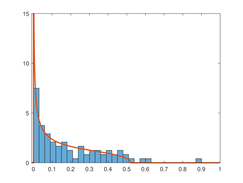
(a) Squared sample canonical correlations between cyclical and non-cyclical stocks (blue columns) and Wachter distribution (orange curve).

	$z_{\rho}$	$\rho^{2}$	$|\rho|$	Angle (in degrees)	Sine squared
$1$st signal	$0.89$	$0.84$	$0.92$	$10.8$	$0.03$
$2$nd signal	$0.62$	$0.43$	$0.65$	$31.0$	$0.27$
$3$rd signal	$0.58$	$0.34$	$0.59$	$38.2$	$0.38$

(b) Strength of the signals and respective vector estimation precision.

Figure 7. Results of CCA performed on cyclical vs. non-cyclical stocks.

We use weekly returns (which are widely believed to be uncorrelated across time) for the $80$ largest cyclical and $80$ largest non-cyclical stocks over ten years ($01.01.2010-01.01.2020$), which gives us $521$ observations across time. The time window is chosen to exclude the $2007-2008$ financial crisis and COVID-19 periods. The exact list of stocks is reported in Appendix C. Figure 7(a) shows the squared sample canonical correlations between the returns of the two groups of stocks. We can see that the overall shape of the histogram of the correlations matches the Wachter distribution (as discussed in Section 2.4, this indicates that the data matches our modelling assumptions and we can use the formulas of Theorem 3.7) and, at the same time, that the three largest correlations are clearly separated from the rest. The largest squared sample canonical correlation, which is close to $0.9$, represents a very strong signal, which can be interpreted as an overall market movement. In favor of this interpretation is also the fact that the majority of the coordinates in the corresponding pair of eigenvectors are positive. For the cyclicals, the sum of squares of the positive coordinates is $0.85$ out of $1$, and for the noncyclicals, it is $0.78$ out of $1$. Two other correlations represent medium-strength signals. The presence of exactly three signals is interesting for several reasons. First, it is resonant of the three factors of Fama and French (1992). Second, it is in noticeable contrast to the results of a principal component analysis (PCA) applied to the same stock returns. PCA often shows few or even only one clearly distinct factor for a large group of stocks; see, e.g., Potters and Bouchaud (2020, 20.4.2 A One-Factor Model). For our two groups of stocks, PCA indicates the presence of at most two factors—fewer than what we detect with CCA. Figure 10 in Appendix C shows the PCA eigenvalues, i.e., eigenvalues of $(\mathbf{V}\mathbf{V}^{\mathsf{T}})/S$ and $(\mathbf{U}\mathbf{U}^{\mathsf{T}})/S$, where $\mathbf{V}$ and $\mathbf{U}$ are the de-meaned cyclical and non-cyclical returns, respectively. We can see that the cyclicals have only one strong factor while the non-cyclicals have two. As with CCA, the largest eigenvalue in PCA is believed to be market related. In our stock returns data set, the largest factors are highly correlated across the two groups (the correlation is $0.83$) and with their CCA counterparts (the first pair of canonical variables). The two other CCA pairs of canonical variables are capturing additional information (cf. the size and value factors in Fama and French (1992)) not reflected by PCA. Based on the above, we observe that CCA picks up more information than PCA by extracting additional relevant factors.

The exact values of the CCA signals are reported in Table 7(b). The correlations and angles in Table 7(b) are calculated based on the results of Theorem 3.7. Since we have $K=M=80$, the angles are the same for the cyclicals and non-cyclicals, and we report only one angle per signal. In line with the strength of the signals, the angle between the first estimated signal and the unobserved truth is the smallest, showing precise estimation. The two other signals are weaker, leading to larger angles, i.e., large estimation error. This observation is reinforced by Figure 8, which shows a scatter plot of the cyclical vs. non-cyclical canonical variables. The points in Figure 8(a) show the tightest fit to the $45$-degree line, demonstrating a very strong correlation, while those in Figures 8(b) and 8(c) are more spread out. The tightness in Figures 8(b) and 8(c) is approximately the same, in line with the second- and third-largest eigenvalues being very close.

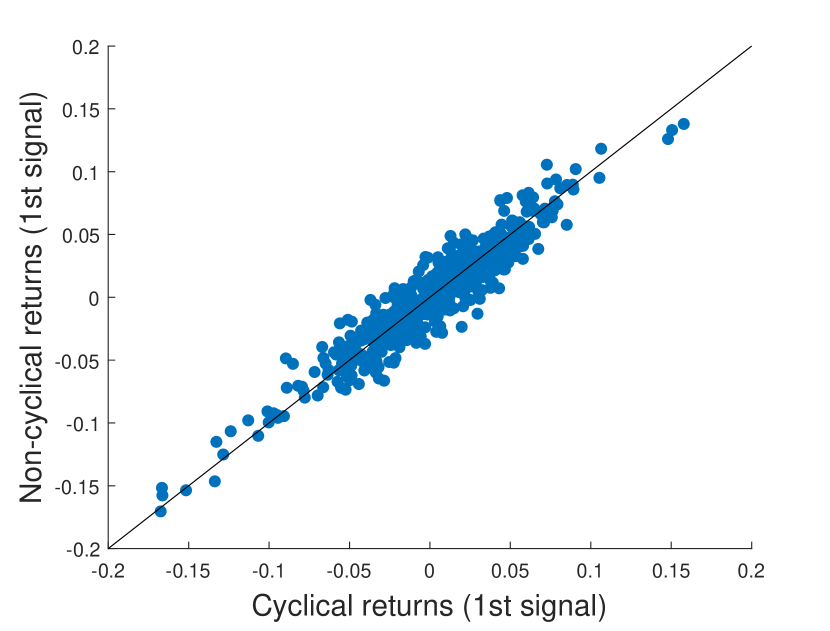
(a) First signal.

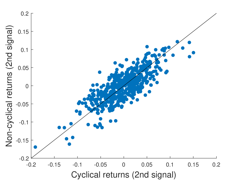
(b) Second signal.

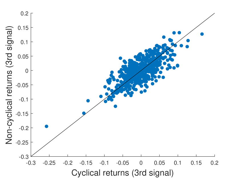
(c) Third signal.

Figure 8. Scatter plot of 521 points $(\mathbf{V}^{\mathsf{T}}\widehat{\boldsymbol{\beta}}^{i},\,\mathbf{U}^{\mathsf{T}}\widehat{\boldsymbol{\alpha}}^{i})$, where matrix $\mathbf{V}$ is composed of cyclical stock returns and matrix $\mathbf{U}$ of non-cyclical stock returns and $i=1,2,3$ is the number of the signal. The length of $\mathbf{V}^{\mathsf{T}}\widehat{\boldsymbol{\beta}}^{i}$ and $\mathbf{U}^{\mathsf{T}}\widehat{\boldsymbol{\alpha}}^{i}$ is normalized to $1$.

4.2. The limestone grassland community data

	Eigenvector	Angle	Sine
		(in degrees)	squared
$\widehat{\boldsymbol{\alpha}},\,\theta_{x},\,\mathfrak{s}_{x}$	$(-0.30,-0.49,-0.80,-0.08,0.15,0.09)$	$14.21$	$0.06$
$\widehat{\boldsymbol{\beta}},\,\theta_{y},\,\mathfrak{s}_{y}$	$(0.77,0.51,0.16,0.10,-0.10,0.15,0.12,-0.25)$	$15.77$	$0.07$

Table 1. Limestone grassland community: CCA. Eigenvectors are obtained from the data, while angles are calculated based on Theorem 2.5.

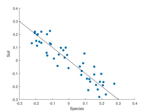
Figure 9. Scatter plot of 45 points $(\mathbf{V}^{\mathsf{T}}\widehat{\boldsymbol{\beta}},\,\mathbf{U}^{\mathsf{T}}\widehat{\boldsymbol{\alpha}})$, where matrix $\mathbf{V}$ is composed of plant species and matrix $\mathbf{U}$ of soil properties. The length of $\mathbf{V}^{\mathsf{T}}\widehat{\boldsymbol{\beta}}^{i}$ and $\mathbf{U}^{\mathsf{T}}\widehat{\boldsymbol{\alpha}}^{i}$ is normalized to $1$.

One of the classic data sets examined by CCA is the limestone grassland community data from Anglesey, North Wales (Gittins (1985)); for instance, these data were discussed recently in Bao et al. (2019). The goal of the CCA application in this case is to identify the relationship between several soil properties and the representation of plant species. There are $M=8$ species considered—Helictotrichon pubescens, Trifolium pratense, Poterium sanguisorba, Phleum bertolonii, Rhytidiadelphus squarrosus, Hieracium pilosella, Briza media, and Thymus drucei—and $K=6$ soil characteristics—depth ($d$), extractable phosphate ($P$), exchangeable potassium ($K$), and cross-product terms between all three soil variables ($d\times P,\,d\times K,\,P\times K$). The number of random samples is $S=45$. To analyze the data, we first de-mean all the variables (the means are calculated across $S$-space). After that we find that the six nonzero squared canonical correlations are $0.83,0.52,0.36,0.11,0.09,0.04$, and we have $\lambda_{+}=0.53$, which indicates the presence of a rank $1$ signal. This signal has estimated strength $|\rho|=0.86$ or $\rho^{2}=0.75$. As can be seen from Table 1, the estimation precision is quite high; i.e., angles $\theta_{x}$ and $\theta_{y}$ are small (the angles are obtained via Theorem 2.5). The estimated vectors $\widehat{\boldsymbol{\alpha}}$ and $\widehat{\boldsymbol{\beta}}$ suggest that most of the correlation comes from the first coordinate of $\widehat{\boldsymbol{\beta}}$ (Helictotrichon pubescens) and the third coordinate of $\widehat{\boldsymbol{\alpha}}$ (potassium). That is, more potassium in the soil is strongly correlated with the presence of Helictotrichon pubescens. Figure 9 shows a scatter plot of $(\mathbf{U}^{\mathsf{T}}\widehat{\boldsymbol{\alpha}},\,\mathbf{V}^{\mathsf{T}}\widehat{\boldsymbol{\beta}})$. As we can see, the data points lie close to the $-45$-degree line, which indicates a correlation close to $-1$.

5. Conclusion

High-dimensional econometrics and statistics have been playing an increasingly prominent role in the analysis of data in social sciences (see, e.g., Fan et al. (2011)). One popular methods for dealing with two large data sets is canonical correlation analysis (CCA). However, little is known about the performance of CCA in the high-dimensional setting where all dimensions of data are large and comparable. This paper provides one of the first results on the precision of CCA in high dimensions. To be more precise, we show that estimation of canonical vectors is inconsistent and compute the exact degree of inconsistency in terms of angles between the true and estimated canonical variables. Consistency can be restored as one of the dimensions becomes much larger than the others.

There are various directions for future research on high-dimensional CCA. The first important generalization is to allow for full correlation across $S$ in the data, i.e., for a setting where both the signal and the noise are dependent across the $S$ dimension. This extension will make the results useful for a typical time series setting, where the coordinate $S$ represents time. One would hope that for stationary time series results in line with Theorem 3.4 continue to hold. An interesting application would be to then use the procedure on the FRED-MD macro time series data set (McCracken and Ng (2016)) and look for canonical correlations between real and nominal variables. Generally, the traditional approach to searching for factors in the FRED-MD data is principal component analysis (PCA). However, this approach does not use any additional information on the type of each variable; i.e., real and nominal variables are mixed together. CCA applied to a subset of real variables vs. a subset of nominal variables can potentially provide another “common” factor.

Another noteworthy area of interest concerns deriving the asymptotic distribution of the angles $\theta_{x}$ and $\theta_{y}$—this would require developing a version of a central limit theorem. An asymptotic distribution of the angles can be required for various procedures that use angles as an input (such as confidence interval construction, the delta method, and simulation of bootstrap standard errors).

Finally, a more refined analysis of what is happening near the identification boundary $\rho^{2}>\tfrac{1}{\sqrt{(\tau_{M}-1)(\tau_{K}-1)}}$ in the spirit of local to unit root limit theory is of theoretical interest. We expect that novel equations involving random functions should appear in the process of answering this question.

Appendix A The master equation

The proofs of all our theorems are based on the master equation — an exact equation satisfied by the canonical correlations and corresponding variables. For illustration purpose, we start by presenting the main ideas for developing such an equation in a simpler setting of principal component analysis (PCA) in Appendix A.1. We then proceed to the canonical correlation analysis (CCA) situation of our main interest in Appendix A.2. Appendix B analyzes these equations as the dimensions go to infinity jointly and proportionally.

A.1. PCA master equation

Suppose that we are given $N\times S$ matrix $\mathbf{U}$, in which the rows are indexed by $i=0,1,\dots,N-1$ and $S\geq N$. We treat the $0$–th row as “signal” and the remaining $N-1$ rows as “noise”. Let $\widetilde{\mathbf{U}}$ denote the latter, i.e., it is the $(N-1)\times S$ matrix formed by rows $i=1,2,\dots,N-1$ of $\mathbf{U}$. As for the former, we let $\lambda_{*}$ denote the length of the zeroth row of $\mathbf{U}$ (treated as a $S$–dimensional vector) and let $\mathbf{u}^{*}$ be the unit vector in the direction of this row.

We would like to connect the singular values and singular vectors of $\mathbf{U}$ to the triplet: singular values and vectors of $\widetilde{\mathbf{U}}$; $\lambda_{*}$; and $\mathbf{u}^{*}$. The goal is to view this connection through the lenses of reconstruction of $\lambda_{*}$ and $\mathbf{u}^{*}$ by the singular values and vectors of $\mathbf{U}$.

Because the singular values are invariant under orthogonal transformations in $N$–dimensional space, the fact that “signal” is the $0$th row of $\mathbf{U}$ is not important: it could have been any other row or their linear combination. Rephrasing, we would like to understand how the singular value decomposition of $\mathbf{U}$ distinguishes the signal vector from the background noise.

We let $(\mathbf{v}_{i},\mathbf{u}_{i},\lambda_{i})$, $1\leq i\leq N-1$, be the left singular vector (of $(N-1)\times 1$ dimensions), right singular vector (of $S\times 1$ dimensions), singular value triplets for $\widetilde{\mathbf{U}}$, which means that

$$\widetilde{\mathbf{U}}=\begin{pmatrix}\mathbf{v}_{1};\mathbf{v}_{2};\dots;\mathbf{v}_{N-1}\end{pmatrix}\begin{pmatrix}\lambda_{1}&0&\dots\\ 0&\lambda_{2}&0&\\ &0&\ddots\\ &&0&\lambda_{N-1}\end{pmatrix}\begin{pmatrix}\mathbf{u}_{1}^{\mathsf{T}}\\ \mathbf{u}_{2}^{\mathsf{T}}\\ \vdots\\ \mathbf{u}_{N-1}^{\mathsf{T}}\end{pmatrix}=\sum_{i=1}^{N-1}\lambda_{i}\mathbf{v}_{i}\mathbf{u}_{i}^{\mathsf{T}}$$

and $\langle\mathbf{u}_{i},\mathbf{u}_{j}\rangle=\delta_{i=j}$, $\langle\mathbf{v}_{i},\mathbf{v}_{j}\rangle=\delta_{i=j}$. We order the singular values so that $\lambda_{1}\geq\lambda_{2}\geq\dots\geq\lambda_{N-1}\geq 0$.

Next, let $\widehat{\boldsymbol{\alpha}}$ be a left singular vector of $\mathbf{U}$. We represent it through coordinates $(\alpha_{0},\alpha_{1},\dots,\alpha_{N})$ in the orthonormal basis

(20) $$\begin{pmatrix}1\\ 0^{N-1}\end{pmatrix},\quad\begin{pmatrix}0\\ \mathbf{v}_{i}\end{pmatrix},\,1\leq i\leq N-1,$$

of $N$–dimensional space and normalize by $\sum_{i=0}^{N-1}\alpha_{i}^{2}=1$.

Proposition A.1.

Suppose that $\widehat{\boldsymbol{\alpha}}=(\alpha_{0},\alpha_{1},\dots,\alpha_{N-1})$ is a left singular vector of $\mathbf{U}$ in basis (20) and with a squared singular value $a\geq 0$. Then

(21) $$\lambda_{*}^{2}=a\left[1+\sum_{i=1}^{N-1}\frac{\lambda_{i}^{2}\langle\mathbf{u}^{*},\mathbf{u}_{i}\rangle^{2}}{a-\lambda_{i}^{2}}\right]^{-1},\qquad\alpha_{0}^{2}=\left[1+a\dfrac{\sum_{i=1}^{N-1}\frac{\lambda_{i}^{2}\langle\mathbf{u}^{*},\mathbf{u}_{i}\rangle^{2}}{(a-\lambda_{i}^{2})^{2}}}{1+\sum_{i=1}^{N-1}\frac{\lambda_{i}^{2}\langle\mathbf{u}^{*},\mathbf{u}_{i}\rangle^{2}}{a-\lambda_{i}^{2}}}\right]^{-1}.$$

Proof.

Each left singular vector $\widehat{\boldsymbol{\alpha}}$ of $\mathbf{U}$ is an $N\times 1$–dimensional column-vector of unit length, which is an eigenvector of $\mathbf{U}\mathbf{U}^{\mathsf{T}}$; equivalently, this is one of the critical points (on the space of unit vectors) for the quadratic form

$$\widehat{\boldsymbol{\alpha}}\mapsto f(\widehat{\boldsymbol{\alpha}})=\langle\widehat{\boldsymbol{\alpha}},\mathbf{U}\mathbf{U}^{\mathsf{T}}\widehat{\boldsymbol{\alpha}}\rangle=\|\mathbf{U}^{\mathsf{T}}\widehat{\boldsymbol{\alpha}}\|^{2},$$

with the eigenvector of largest eigenvalue corresponding to the maximum of this quadratic form. Then we have

$$f(\widehat{\boldsymbol{\alpha}})=\left\|\alpha_{0}\lambda_{*}\mathbf{u}^{*}+\sum_{i=1}^{N-1}\alpha_{i}\lambda_{i}\mathbf{u}_{i}\right\|^{2}=\alpha_{0}^{2}\lambda_{*}^{2}+2\alpha_{0}\lambda_{*}\sum_{i=1}^{N-1}\alpha_{i}\lambda_{i}\langle\mathbf{u}^{*},\mathbf{u}_{i}\rangle+\sum_{i=1}^{N-1}\alpha_{i}^{2}\lambda_{i}^{2}.$$

We aim to find critical points of $f(\widehat{\boldsymbol{\alpha}})$ subject to the constraint $\|\widehat{\boldsymbol{\alpha}}\|^{2}=\sum_{i=0}^{N-1}\alpha_{i}^{2}=1$. Thus, we introduce the Lagrange multiplier $a$ and find critical points of the function

$$g(\widehat{\boldsymbol{\alpha}},a)=f(\widehat{\boldsymbol{\alpha}})-a\left(\sum_{i=0}^{N-1}\alpha_{i}^{2}-1\right).$$

Taking derivatives with respect to $\alpha$, we get:

(22) $$\begin{dcases}0=\frac{\partial g}{\partial\alpha_{i}}=2\alpha_{0}\lambda_{*}\lambda_{i}\langle\mathbf{u}^{*},\mathbf{u}_{i}\rangle+2\alpha_{i}\lambda_{i}^{2}-2a\alpha_{i},&1\leq i\leq N-1,\\ 0=\frac{\partial g}{\partial\alpha_{0}}=2\alpha_{0}\lambda_{*}^{2}+2\sum_{i=1}^{N-1}\alpha_{i}\lambda_{*}\lambda_{i}\langle\mathbf{u}^{*},\mathbf{u}_{i}\rangle-2a\alpha_{0}.\end{dcases}$$

The equations (22) are supplemented by the normalization condition $\sum_{i=0}^{N-1}\alpha_{i}^{2}=1$. Note that equations (22) equivalently express the fact that $\widehat{\boldsymbol{\alpha}}$ is an eigenvector with eigenvalue $a$ for the matrix $\mathbf{U}\mathbf{U}^{\mathsf{T}}$ written in the orthonormal basis (20). From this interpretation we see that the values of $a$, for which (22) has a solution, are precisely eigenvalues of $\mathbf{U}\mathbf{U}^{\mathsf{T}}$, i.e., squared singular values of $\mathbf{U}$. On the other hand, (22) can be also solved directly. Indeed, the first set of $N-1$ equations leads to

(23) $$\alpha_{i}=\alpha_{0}\frac{\lambda_{*}\lambda_{i}\langle\mathbf{u}^{*},\mathbf{u}_{i}\rangle}{a-\lambda_{i}^{2}},\qquad 1\leq i\leq N-1.$$

Plugging the expressions for $\alpha_{i}$ into the last equation of (22), we get

$$2\alpha_{0}\left(\lambda_{*}^{2}+\lambda_{*}^{2}\sum_{i=1}^{N-1}\frac{\lambda_{i}^{2}\langle\mathbf{u}^{*},\mathbf{u}_{i}\rangle^{2}}{a-\lambda_{i}^{2}}-a\right)=0.$$

If $\alpha_{0}=0$, then so are all $\alpha_{i}$ through (23), which contradicts the $\sum_{i=0}^{N-1}\alpha_{i}^{2}=1$ normalization. Hence, we can divide by $2\alpha_{0}$, arriving at the final equation for $a$:

(24) $$\lambda_{*}^{2}\left(1+\sum_{i=1}^{N-1}\frac{\lambda_{i}^{2}\langle\mathbf{u}^{*},\mathbf{u}_{i}\rangle^{2}}{a-\lambda_{i}^{2}}\right)=a,$$

which is equivalent to the first equation in (21).

In order to compute the corresponding value of $\alpha_{0}$, which is the cosine of the angle between $\widehat{\boldsymbol{\alpha}}$ and the signal direction $(1,0^{N-1})$, plug (23) into the normalization condition $\sum_{i=0}^{N-1}\alpha_{i}^{2}=1$ to get

(25) $$\alpha_{0}^{2}\left(1+\lambda_{*}^{2}\sum_{i=1}^{N-1}\frac{\lambda_{i}^{2}\langle\mathbf{u}^{*},\mathbf{u}_{i}\rangle^{2}}{(a-\lambda_{i}^{2})^{2}}\right)=1$$

Plugging $\lambda_{*}^{2}$ from the first equation in (21), we rewrite (25) as the second equation of (21). ∎

Here is a brief qualitative analysis of the formulas (21). First, let us treat the first equation in (21) in the form (24) as an equation on $a$, assuming that the values of $\lambda_{*}$, $\lambda_{1},\dots,\lambda_{N-1}$ and $\langle\mathbf{u}^{*},\mathbf{u}_{1}\rangle$, …, $\langle\mathbf{u}^{*},\mathbf{u}_{N-1}\rangle$ are known. Let us also assume, for simplicity, that all $\lambda_{i}$ are distinct. After multiplying by $\prod_{i=1}^{N-1}(a-\lambda_{i}^{2})$, the equation (24) becomes a degree $N$ polynomial equation on $a$; hence, it has $N$ complex roots. For each $i=1,2,\dots,N-2$, the difference between right-hand side and left-hand side of (24) continuously varies from $+\infty$ to $-\infty$ on $(\lambda_{i+1}^{2},\lambda_{i}^{2})$ segment; hence there is one root of the equation on each such segment. In addition, by the same sign change argument there is one more root on $[0,\lambda_{N-1})$ and one more root on $(\lambda_{1},+\infty)$. We are mostly interested in the latter two values of $a$, because one can easily distinguish a separated largest/smallest singular value from others, while doing the same for singular values in the bulk of spectrum is challenging.

Next, let us treat the formulas (21) as a parameterization of $\lambda_{*}^{2}$ and $\alpha_{0}^{2}$ by the value of $a$. When we work with data, we know $a$: this is one of the squared singular values of the matrix $\mathbf{U}$. Therefore, it is reasonable to ask what information on (unknown to us) $\lambda_{*}$ and $\alpha_{0}$ it provides. There are two important regimes here:

1. If $a$ is large, then $\lambda_{*}^{2}=a+O(1)$ is also large, while $\alpha_{0}^{2}=1+O(\tfrac{1}{a})$ approaches $1$.

2. If $a$ is close to $0$, then $\lambda_{*}^{2}=O(a)$ is also close to $0$, while $\alpha_{0}^{2}=1+O(a)$ approaches $1$.

On the other hand, for the intermediate values of $a$ and $\lambda_{*}^{2}$, the value of $\alpha_{0}^{2}$ is typically quite far away from $1$. The conclusion is that we can effectively distinguish the signal vector (the zeroth row of $\mathbf{U}$), if its length is either very small or very large, as compared to the values of $\{\lambda_{i}\}_{i=1}^{N}$, which are singular values of the matrix $\widetilde{\mathbf{U}}$ formed by the remaining $N$ rows of $\mathbf{U}$. Recall that $\widetilde{\mathbf{U}}$ represents the noise part; it is, perhaps, strange to ask the noise to be large enough, and much more natural to assume that the noise is small enough. Hence, in practice, the situation of interest is when the length $\lambda_{*}$ of the signal vector is large (rather than small) compared to the magnitude of the noise.

A.2. CCA master equation

We proceed to the canonical correlations analysis setting. Suppose that we are given two subspaces, $\widetilde{\mathbf{U}}$ and $\widetilde{\mathbf{V}}$ in $S$–dimensional space and let $\dim(\widetilde{\mathbf{V}})={M-1}\geq{K-1}=\dim(\widetilde{\mathbf{U}})$. In addition, we have two vectors $\mathbf{u}^{*}$ and $\mathbf{v}^{*}$, which we add to spaces $\widetilde{\mathbf{U}}$ and $\widetilde{\mathbf{V}}$. Define

$$\mathbf{U}=\mathrm{span}(\mathbf{u}^{*},\widetilde{\mathbf{U}}),\qquad\mathbf{V}=\mathrm{span}(\mathbf{v}^{*},\widetilde{\mathbf{V}}).$$

Our task is to reconstruct the vectors $\mathbf{u}^{*}$ and $\mathbf{v}^{*}$ inside the spaces $\mathbf{U}$ and $\mathbf{V}$, respectively, by analyzing the canonical correlations between $\mathbf{U}$ and $\mathbf{V}$.

We start by bringing the pair of subspaces $\widetilde{\mathbf{U}}$ and $\widetilde{\mathbf{V}}$ to the canonical form. The following definitions of canonical correlations and variables can already be found in Hotelling (1936), see bottom of page 330 there. We also refer to the textbook Anderson (2003, Chapter 12).

Lemma A.2.

Suppose that $S>M\geq K$ and let $\widetilde{\mathbf{U}}$ and $\widetilde{\mathbf{V}}$ be ${K-1}$-dimensional and ${M-1}$-dimensional subspaces of $S$ dimensional space, respectively. Then there exist two orthonormal bases: vectors $\mathbf{u}_{1},\mathbf{u}_{2},\dots,\mathbf{u}_{K-1}$ span $\widetilde{\mathbf{U}}$ and vectors $\mathbf{v}_{1},\dots,\mathbf{v}_{M-1}$ span $\widetilde{\mathbf{V}}$ – such that for all meaningful indices $i$ and $j$:

(26) $$\langle\mathbf{u}_{i},\mathbf{u}_{j}\rangle=\delta_{i=j},\qquad\langle\mathbf{v}_{i},\mathbf{v}_{j}\rangle=\delta_{i=j},\qquad\langle\mathbf{u}_{i},\mathbf{v}_{j}\rangle=c_{i}\delta_{i=j},$$

where $1\geq c_{1}\geq c_{2}\geq\dots\geq c_{K-1}\geq 0$.

The numbers $c_{1}\geq c_{2}\geq\dots\geq c_{K-1}$ are called canonical correlation coefficients between subspaces $\widetilde{\mathbf{U}}$ and $\widetilde{\mathbf{V}}$; they are also cosines of the canonical angles between the subspaces. The vectors $\mathbf{u}_{i}$, $1\leq i\leq{K-1}$, and $\mathbf{v}_{j}$, $1\leq k\leq{M-1}$, are called canonical variables; they split into ${K-1}$ pairs $(\mathbf{u}_{i},\mathbf{v}_{i})$ and $M-K$ singletons $v_{j}$, $j\geq K$. In some of the following formulas we also use $c_{j}$ with $j\geq K$ under the convention:

(27) $$c_{K}=c_{{K-1}+2}=\dots=c_{M-1}=0.$$

There are two equivalent ways to find the canonical correlations and variables:

• If we consider a function $f(\mathbf{u},\mathbf{v})=\langle\mathbf{u},\mathbf{v}\rangle$, in which $\mathbf{u}$ varies over all unit vectors in $\widetilde{\mathbf{U}}$ and $\mathbf{v}$ varies over all unit vectors in $\widetilde{\mathbf{V}}$, then $(\mathbf{u}_{i},\mathbf{v}_{i},c_{i})$, $1\leq i\leq{K-1}$, are critical points of $f$ and corresponding values of $f$. In particular, $c_{1}$ is the maximum of $f$, which is achieved at $(\mathbf{u}_{1},\mathbf{v}_{1})$. The remaining vectors $\mathbf{v}_{j}$, $j>{K-1}$ are an arbitrary orthogonal basis in the part of $\widetilde{\mathbf{V}}$ orthogonal to all vectors of $\widetilde{\mathbf{U}}$ and $\mathbf{v}_{1},\dots,\mathbf{v}_{K-1}$.

• For a subspace $W$, let us denote through $P_{W}$ the orthogonal projector on $W$. Then nonzero $c_{i}^{2}$, $1\leq i\leq{K-1}$ are nonzero eigenvalues of $P_{\widetilde{\mathbf{U}}}P_{\widetilde{\mathbf{V}}}P_{\widetilde{\mathbf{U}}}$ and $\mathbf{u}_{i}$ are corresponding eigenvectors. Simultaneously, nonzero $c_{i}^{2}$ are eigenvalues of $P_{\widetilde{\mathbf{V}}}P_{\widetilde{\mathbf{U}}}P_{\widetilde{\mathbf{V}}}$. If we identify the spaces $\widetilde{\mathbf{U}}$ and $\widetilde{\mathbf{V}}$ with spans of rows of $(K-1)\times S$ and $(M-1)\times S$ matrices, then this is equivalent to Definition 2.4.

Throughout the rest of this section we use the bases of Lemma A.2.

In exactly the same fashion we can also define the canonical correlation coefficients and corresponding variables for the spaces $\mathbf{U}$ and $\mathbf{V}$. The next theorem connects them to $\mathbf{u}^{*}$, $\mathbf{v}^{*}$ and the data of Lemma A.2

Take two vectors $\widehat{\boldsymbol{\alpha}}=(\alpha_{0},\alpha_{1},\dots,\alpha_{K-1})$ and $\widehat{\boldsymbol{\beta}}=(\beta_{0},\beta_{1},\dots,\beta_{M-1})$, such that $\alpha_{0}\mathbf{u}^{*}+\sum_{i=1}^{K-1}\alpha_{i}\mathbf{u}_{i}$ and $\beta_{0}\mathbf{v}^{*}+\sum_{j=1}^{M-1}\beta_{j}\mathbf{v}_{j}$ is a pair of canonical variables for $\mathbf{U}$ and $\mathbf{V}$. We normalize the vectors so that

(28) $$\left\|\alpha_{0}\mathbf{u}^{*}+\sum_{i=1}^{K-1}\alpha_{i}\mathbf{u}_{i}\right\|^{2}=\left\|\beta_{0}\mathbf{v}^{*}+\sum_{j=1}^{M-1}\beta_{j}\mathbf{v}_{j}\right\|^{2}=1.$$

The next theorem is a direct analogue of Proposition A.1 in the CCA setting.

Theorem A.3.

Take two vectors $\widehat{\boldsymbol{\alpha}}$, $\widehat{\boldsymbol{\beta}}$ normalized as in (28) and such that $\alpha_{0}\mathbf{u}^{*}+\sum_{i=1}^{K-1}\alpha_{i}\mathbf{u}_{i}$ and $\beta_{0}\mathbf{v}^{*}+\sum_{j=1}^{M-1}\beta_{j}\mathbf{v}_{j}$ is a pair of canonical variables for $\mathbf{U}$ and $\mathbf{V}$ with squared canonical correlation coefficient $z=\left\langle\alpha_{0}\mathbf{u}^{*}+\sum_{i=1}^{K-1}\alpha_{i}\mathbf{u}_{i},\,\beta_{0}\mathbf{v}^{*}+\sum_{j=1}^{M-1}\beta_{j}\mathbf{v}_{j}\right\rangle^{2}$. Then we have

(29) $$\left[\langle\mathbf{u}^{*},\mathbf{v}^{*}\rangle+\sum_{j=1}^{M-1}\frac{\langle\mathbf{u}^{*},\mathbf{v}_{j}\rangle(c_{j}\langle\mathbf{v}^{*},\mathbf{u}_{j}\rangle-z\langle\mathbf{v}^{*},\mathbf{v}_{j}\rangle)}{z-c_{j}^{2}}-z\sum_{i=1}^{K-1}\frac{\langle\mathbf{u}^{*},\mathbf{u}_{i}\rangle(\langle\mathbf{v}^{*},\mathbf{u}_{i}\rangle-c_{i}\langle\mathbf{v}^{*},\mathbf{v}_{i}\rangle)}{z-c_{i}^{2}}\right]^{2}\\ =z\left[-\langle\mathbf{u}^{*},\mathbf{u}^{*}\rangle+\sum_{j=1}^{M-1}\frac{\langle\mathbf{u}^{*},\mathbf{v}_{j}\rangle^{2}-2c_{j}\langle\mathbf{u}^{*},\mathbf{v}_{j}\rangle\langle\mathbf{u}^{*},\mathbf{u}_{j}\rangle}{z-c_{j}^{2}}+z\sum_{i=1}^{K-1}\frac{\langle\mathbf{u}^{*},\mathbf{u}_{i}\rangle^{2}}{z-c_{i}^{2}}\right]\\ \times\left[-\langle\mathbf{v}^{*},\mathbf{v}^{*}\rangle+\sum_{i=1}^{K-1}\frac{\langle\mathbf{v}^{*},\mathbf{u}_{i}\rangle^{2}-2c_{i}\langle\mathbf{v}^{*},\mathbf{u}_{i}\rangle\langle\mathbf{v}^{*},\mathbf{v}_{i}\rangle}{z-c_{i}^{2}}+z\sum_{j=1}^{M-1}\frac{\langle\mathbf{v}^{*},\mathbf{v}_{j}\rangle^{2}}{z-c_{j}^{2}}\right],$$

where we used the convention (27), and

$$\frac{1}{\alpha_{0}^{2}}=\langle\mathbf{u}^{*},\mathbf{u}^{*}\rangle +2\sum_{i=1}^{K-1}\frac{\langle\mathbf{u}^{*},\mathbf{u}_{i}\rangle}{z-c_{i}^{2}}\Bigl{[}c_{i}\langle\mathbf{u}^{*},\mathbf{v}_{i}\rangle-z\langle\mathbf{u}^{*},\mathbf{u}_{i}\rangle-z\mathfrak{Q}_{\alpha}(z)\bigl{(}\langle\mathbf{v}^{*},\mathbf{u}_{i}\rangle-c_{i}\langle\mathbf{v}^{*},\mathbf{v}_{i}\rangle\bigr{)}\Bigr{]}$$

(30) $$+\sum_{i=1}^{K-1}\frac{1}{(z-c_{i}^{2})^{2}}\Bigl{[}c_{i}\langle\mathbf{u}^{*},\mathbf{v}_{i}\rangle-z\langle\mathbf{u}^{*},\mathbf{u}_{i}\rangle-z\mathfrak{Q}_{\alpha}(z)\bigl{(}\langle\mathbf{v}^{*},\mathbf{u}_{i}\rangle-c_{i}\langle\mathbf{v}^{*},\mathbf{v}_{i}\rangle\bigr{)}\Bigr{]}^{2},$$

$$\frac{1}{\beta_{0}^{2}}=\langle\mathbf{v}^{*},\mathbf{v}^{*}\rangle +2\sum_{j=1}^{M-1}\frac{\langle\mathbf{v}^{*},\mathbf{v}_{j}\rangle}{z-c_{j}^{2}}\Bigl{[}-z\mathfrak{Q}_{\beta}(z)\bigl{(}\langle\mathbf{u}^{*},\mathbf{v}_{j}\rangle-c_{j}\langle\mathbf{u}^{*},\mathbf{u}_{j}\rangle\bigr{)}+c_{j}\langle\mathbf{v}^{*},\mathbf{u}_{j}\rangle-z\langle\mathbf{v}^{*},\mathbf{v}_{j}\rangle\Bigr{]}$$

(31) $$+\sum_{j=1}^{M-1}\frac{1}{(z-c_{j}^{2})^{2}}\Bigl{[}-z\mathfrak{Q}_{\beta}(z)\bigl{(}\langle\mathbf{u}^{*},\mathbf{v}_{j}\rangle-c_{j}\langle\mathbf{u}^{*},\mathbf{u}_{j}\rangle\bigr{)}+c_{j}\langle\mathbf{v}^{*},\mathbf{u}_{j}\rangle-z\langle\mathbf{v}^{*},\mathbf{v}_{j}\rangle\Bigr{]}^{2},$$

and

(32) $$\left\langle\mathbf{u}^{*},\,\alpha_{0}\mathbf{u}^{*}+\sum_{i=1}^{K-1}\alpha_{i}\mathbf{u}_{i}\right\rangle\\ =\alpha_{0}\Biggl{(}\langle\mathbf{u}^{*},\mathbf{u}^{*}\rangle+\sum_{i=1}^{K-1}\frac{\langle\mathbf{u}^{*},\mathbf{u}_{i}\rangle}{z-c_{i}^{2}}\Bigl{[}c_{i}\langle\mathbf{u}^{*},\mathbf{v}_{i}\rangle-z\langle\mathbf{u}^{*},\mathbf{u}_{i}\rangle-z\mathfrak{Q}_{\alpha}(z)\bigl{(}\langle\mathbf{v}^{*},\mathbf{u}_{i}\rangle-c_{i}\langle\mathbf{v}^{*},\mathbf{v}_{i}\rangle\bigr{)}\Bigr{]}\Biggr{)},$$

(33) $$\left\langle\mathbf{v}^{*},\,\beta_{0}\mathbf{v}^{*}+\sum_{j=1}^{M-1}\beta_{i}\mathbf{v}_{i}\right\rangle\\ =\beta_{0}\Biggl{(}\langle\mathbf{v}^{*},\mathbf{v}^{*}\rangle+\sum_{j=1}^{M-1}\frac{\langle\mathbf{v}^{*},\mathbf{v}_{j}\rangle}{z-c_{j}^{2}}\Bigl{[}-z\mathfrak{Q}_{\beta}(z)\bigl{(}\langle\mathbf{u}^{*},\mathbf{v}_{j}\rangle-c_{j}\langle\mathbf{u}^{*},\mathbf{u}_{j}\rangle\bigr{)}+c_{j}\langle\mathbf{v}^{*},\mathbf{u}_{j}\rangle-z\langle\mathbf{v}^{*},\mathbf{v}_{j}\rangle\Bigr{]}\Biggr{)},$$

where

(34) $$\mathfrak{Q}_{\alpha}(z):=\frac{-\langle\mathbf{u}^{*},\mathbf{u}^{*}\rangle+\sum_{j=1}^{M-1}\frac{\langle\mathbf{u}^{*},\mathbf{v}_{j}\rangle^{2}-2c_{j}\langle\mathbf{u}^{*},\mathbf{v}_{j}\rangle\langle\mathbf{u}^{*},\mathbf{u}_{j}\rangle}{z-c_{j}^{2}}+z\sum_{i=1}^{K-1}\frac{\langle\mathbf{u}^{*},\mathbf{u}_{i}\rangle^{2}}{z-c_{i}^{2}}}{\langle\mathbf{u}^{*},\mathbf{v}^{*}\rangle+\sum_{j=1}^{M-1}\frac{\langle\mathbf{u}^{*},\mathbf{v}_{j}\rangle(c_{j}\langle\mathbf{v}^{*},\mathbf{u}_{j}\rangle-z\langle\mathbf{v}^{*},\mathbf{v}_{j}\rangle)}{z-c_{j}^{2}}-z\sum_{i=1}^{K-1}\frac{\langle\mathbf{u}^{*},\mathbf{u}_{i}\rangle(\langle\mathbf{v}^{*},\mathbf{u}_{i}\rangle-c_{i}\langle\mathbf{v}^{*},\mathbf{v}_{i}\rangle)}{z-c_{i}^{2}}},$$

(35) $$\mathfrak{Q}_{\beta}(z):=\frac{-\langle\mathbf{v}^{*},\mathbf{v}^{*}\rangle+\sum_{i=1}^{K-1}\frac{\langle\mathbf{v}^{*},\mathbf{u}_{i}\rangle^{2}-2c_{i}\langle\mathbf{v}^{*},\mathbf{u}_{i}\rangle\langle\mathbf{v}^{*},\mathbf{v}_{i}\rangle}{z-c_{i}^{2}}+z\sum_{j=1}^{M-1}\frac{\langle\mathbf{v}^{*},\mathbf{v}_{j}\rangle^{2}}{z-c_{j}^{2}}}{\langle\mathbf{u}^{*},\mathbf{v}^{*}\rangle+\sum_{i=1}^{K-1}\frac{\langle\mathbf{v}^{*},\mathbf{u}_{i}\rangle(c_{i}\langle\mathbf{u}^{*},\mathbf{v}_{i}\rangle-z\langle\mathbf{u}^{*},\mathbf{u}_{i}\rangle)}{z-c_{i}^{2}}-z\sum_{j=1}^{M-1}\frac{\langle\mathbf{v}^{*},\mathbf{v}_{j}\rangle(\langle\mathbf{u}^{*},\mathbf{v}_{j}\rangle-c_{j}\langle\mathbf{u}^{*},\mathbf{u}_{j}\rangle)}{z-c_{j}^{2}}}.$$

Remark A.4.

Comparing to the PCA setting, (29) is an analogue of the first equation in (21) and (30), (31) are analogues of the second equation in (21). A version of (32), (33) for the PCA would be the computation of the scalar product between $\mathbf{u}^{*}$ and the right singular vector corresponding to the singular value $a$, which we omitted there.

Proof of Theorem A.3.

We seek for a pair of vectors $\widehat{\boldsymbol{\alpha}}=(\alpha_{0},\alpha_{1},\dots,\alpha_{K-1})$ and $\widehat{\boldsymbol{\beta}}=(\beta_{0},\beta_{1},\dots,\beta_{M-1})$, which represent critical points of the function

$$f(\widehat{\boldsymbol{\alpha}},\widehat{\boldsymbol{\beta}})=\left\langle\alpha_{0}\mathbf{u}^{*}+\sum_{i=1}^{K-1}\alpha_{i}\mathbf{u}_{i},\,\beta_{0}\mathbf{v}^{*}+\sum_{j=1}^{M-1}\beta_{j}\mathbf{v}_{j}\right\rangle,$$

subject to the normalization constraints

(36) $$\left\|\alpha_{0}\mathbf{u}^{*}+\sum_{i=1}^{K-1}\alpha_{i}\mathbf{u}_{i}\right\|^{2}=\left\|\beta_{0}\mathbf{v}^{*}+\sum_{j=1}^{M-1}\beta_{j}\mathbf{v}_{j}\right\|^{2}=1.$$

In this way, $\alpha_{0}\mathbf{u}^{*}+\sum_{i=1}^{K-1}\alpha_{i}\mathbf{u}_{i}$, $\beta_{0}\mathbf{v}^{*}+\sum_{j=1}^{M-1}\beta_{j}\mathbf{v}_{j}$ is a pair of canonical variables for $\mathbf{U}$ and $\mathbf{V}$ and the corresponding value of $f(\widehat{\boldsymbol{\alpha}},\widehat{\boldsymbol{\beta}})$ is a canonical correlation coefficient.

Introducing the Lagrange multipliers $a$ and $b$ corresponding to two normalizations (36), we are led to the Lagrangian function

(37) $$g(\widehat{\boldsymbol{\alpha}},\widehat{\boldsymbol{\beta}},a,b)=\alpha_{0}\beta_{0}\langle\mathbf{u}^{*},\mathbf{v}^{*}\rangle+\alpha_{0}\sum_{j=1}^{M-1}\beta_{j}\langle\mathbf{u}^{*},\mathbf{v}_{j}\rangle+\beta_{0}\sum_{i=1}^{K-1}\alpha_{i}\langle\mathbf{v}^{*},\mathbf{u}_{i}\rangle+\sum_{i=1}^{K-1}\alpha_{i}\beta_{i}c_{i}\\ -a\left(\alpha_{0}^{2}\langle\mathbf{u}^{*},\mathbf{u}^{*}\rangle+2\alpha_{0}\sum_{i=1}^{K-1}\alpha_{i}\langle\mathbf{u}^{*},\mathbf{u}_{i}\rangle+\sum_{i=1}^{K-1}\alpha_{i}^{2}-1\right)\\ -b\left(\beta_{0}^{2}\langle\mathbf{v}^{*},\mathbf{v}^{*}\rangle+2\beta_{0}\sum_{j=1}^{M-1}\beta_{j}\langle\mathbf{v}^{*},\mathbf{v}_{j}\rangle+\sum_{j=1}^{M-1}\beta_{j}^{2}-1\right).$$

We need to find critical points of this function. Differentiating with respect to $\alpha_{i}$ and $\beta_{j}$, we get a system of $K+M$ homogeneous linear equations on coordinates of $\widehat{\boldsymbol{\alpha}}$ and $\widehat{\boldsymbol{\beta}}$:

(38) $$\begin{dcases}0=\frac{\partial g}{\partial\alpha_{0}}=\beta_{0}\langle\mathbf{u}^{*},\mathbf{v}^{*}\rangle+\sum_{j=1}^{M-1}\beta_{j}\langle\mathbf{u}^{*},\mathbf{v}_{j}\rangle-2a\alpha_{0}\langle\mathbf{u}^{*},\mathbf{u}^{*}\rangle-2a\sum_{i=1}^{K-1}\alpha_{i}\langle\mathbf{u}^{*},\mathbf{u}_{i}\rangle,\\ 0=\frac{\partial g}{\partial\alpha_{i}}=\beta_{0}\langle\mathbf{v}^{*},\mathbf{u}_{i}\rangle+\beta_{i}c_{i}-2a\alpha_{0}\langle\mathbf{u}^{*},\mathbf{u}_{i}\rangle-2a\alpha_{i},&1\leq i<K,\\ 0=\frac{\partial g}{\partial\beta_{0}}=\alpha_{0}\langle\mathbf{u}^{*},\mathbf{v}^{*}\rangle+\sum_{i=1}^{K-1}\alpha_{i}\langle\mathbf{v}^{*},\mathbf{u}_{i}\rangle-2b\beta_{0}\langle\mathbf{v}^{*},\mathbf{v}^{*}\rangle-2b\sum_{j=1}^{M-1}\beta_{j}\langle\mathbf{v}^{*},\mathbf{v}_{j}\rangle,\\ 0=\frac{\partial g}{\partial\beta_{j}}=\alpha_{0}\langle\mathbf{u}^{*},\mathbf{v}_{j}\rangle+\delta_{j<K}\cdot\alpha_{j}c_{j}-2b\beta_{0}\langle\mathbf{v}^{*},\mathbf{v}_{j}\rangle-2b\beta_{j},&1\leq j<M.\\ \end{dcases}$$

In the matrix form, the equations (38) can be rewritten as

(39) $$\begin{cases}S_{uv}\widehat{\boldsymbol{\beta}}=2aS_{uu}\widehat{\boldsymbol{\alpha}},\\ S_{vu}\widehat{\boldsymbol{\alpha}}=2bS_{vv}\widehat{\boldsymbol{\beta}},\end{cases}$$

where $\widehat{\boldsymbol{\alpha}}$ and $\widehat{\boldsymbol{\beta}}$ are treated as column-vectors of sizes $K\times 1$ and $M\times 1$, respectively, and $S_{\cdot\cdot}$ are matrices of scalar products:

(40) $$[S_{uv}]_{i,j}=[S_{v}u]_{j,i}=\langle\mathbf{u}_{i},\mathbf{v}_{j}\rangle,\qquad[S_{uu}]_{i,i^{\prime}}=\langle\mathbf{u}_{i},\mathbf{u}_{i^{\prime}}\rangle,\qquad[S_{vv}]_{j,j^{\prime}}=\langle\mathbf{v}_{j},\mathbf{v}_{j^{\prime}}\rangle,$$

with $0\leq i,i^{\prime}\leq{K-1}$, $0\leq j,j^{\prime}\leq{M-1}$. Note that (39) implies eigenrelations

(41) $$\begin{cases}(S_{vv})^{-1}S_{vu}(S_{uu})^{-1}S_{uv}\,\widehat{\boldsymbol{\beta}}=4ab\,\widehat{\boldsymbol{\beta}},\\ (S_{uu})^{-1}S_{uv}(S_{vv})^{-1}S_{vu}\,\widehat{\boldsymbol{\alpha}}=4ab\,\widehat{\boldsymbol{\alpha}}.\end{cases}$$

Comparing (41) with standard algorithms for finding canonical correlations as in Definition 2.4, we conclude that $4ab$ should necessary be one of the squared sample canonical correlations between spaces $\mathbf{U}$ and $\mathbf{V}$. On the other hand, the equations (38) can be solved directly. We first combine the second and the forth equation for $i=j\leq{K-1}$ and treat the result as a system of two linear equations on the variables $(\alpha_{i},\beta_{i})$:

(42) $$\begin{cases}-2a\alpha_{i}+c_{i}\beta_{i}&=\,\,2a\alpha_{0}\langle\mathbf{u}^{*},\mathbf{u}_{i}\rangle-\beta_{0}\langle\mathbf{v}^{*},\mathbf{u}_{i}\rangle,\\ \,\,\,\,\,c_{i}\alpha_{i}-2b\beta_{i}&=\,\,-\alpha_{0}\langle\mathbf{u}^{*},\mathbf{v}_{i}\rangle+2b\beta_{0}\langle\mathbf{v}^{*},\mathbf{v}_{i}\rangle.\end{cases}$$

We solve these equation by inverting the $2\times 2$ matrix in the left-hand side:

$$\begin{pmatrix}-2a&c_{i}\\ c_{i}&-2b\end{pmatrix}^{-1}=\frac{1}{4ab-c_{i}^{2}}\begin{pmatrix}-2b&-c_{i}\\ -c_{i}&-2a\end{pmatrix}.$$

Multiplying by the right-hand side of (42), the solution is

(43) $$\begin{dcases}\alpha_{i}=\frac{1}{4ab-c_{i}^{2}}\Bigl{[}\bigl{(}c_{i}\langle\mathbf{u}^{*},\mathbf{v}_{i}\rangle-4ab\langle\mathbf{u}^{*},\mathbf{u}_{i}\rangle\bigr{)}\cdot\alpha_{0}&+\quad\bigl{(}\langle\mathbf{v}^{*},\mathbf{u}_{i}\rangle-c_{i}\langle\mathbf{v}^{*},\mathbf{v}_{i}\rangle\bigr{)}\cdot 2b\cdot\beta_{0}\Bigr{]},\\ \beta_{i}=\frac{1}{4ab-c_{i}^{2}}\Bigl{[}\bigl{(}\langle\mathbf{u}^{*},\mathbf{v}_{i}\rangle-c_{i}\langle\mathbf{u}^{*},\mathbf{u}_{i}\rangle\bigr{)}\cdot 2a\cdot\alpha_{0}&+\quad\bigl{(}c_{i}\langle\mathbf{v}^{*},\mathbf{u}_{i}\rangle-4ab\langle\mathbf{v}^{*},\mathbf{v}_{i}\rangle\bigr{)}\cdot\beta_{0}\Bigr{]}.\end{dcases}$$

In addition, for $K\leq j<M$, we rewrite the last equation of (38) in a similar form:

(44) $$\beta_{j}=\frac{1}{4ab}\Bigl{[}\langle\mathbf{u}^{*},\mathbf{v}_{j}\rangle\cdot 2a\cdot\alpha_{0}-4ab\langle\mathbf{v}^{*},\mathbf{v}_{j}\rangle\cdot\beta_{0}\Bigr{]},$$

which can be thought of as the second equation of (43) with $c_{j}=0$. Next, we plug (43) and (44) back into the first and third equations of (38) and get:

(45) $$\alpha_{0}\cdot 2a\cdot\left[-\langle\mathbf{u}^{*},\mathbf{u}^{*}\rangle+\sum_{j=1}^{M-1}\frac{\langle\mathbf{u}^{*},\mathbf{v}_{j}\rangle^{2}-2c_{j}\langle\mathbf{u}^{*},\mathbf{v}_{j}\rangle\langle\mathbf{u}^{*},\mathbf{u}_{j}\rangle}{4ab-c_{j}^{2}}+4ab\sum_{i=1}^{K-1}\frac{\langle\mathbf{u}^{*},\mathbf{u}_{i}\rangle^{2}}{4ab-c_{i}^{2}}\right]\\ +\beta_{0}\left[\langle\mathbf{u}^{*},\mathbf{v}^{*}\rangle+\sum_{j=1}^{M-1}\frac{\langle\mathbf{u}^{*},\mathbf{v}_{j}\rangle(c_{j}\langle\mathbf{v}^{*},\mathbf{u}_{j}\rangle-4ab\langle\mathbf{v}^{*},\mathbf{v}_{j}\rangle)}{4ab-c_{j}^{2}}-4ab\sum_{i=1}^{K-1}\frac{\langle\mathbf{u}^{*},\mathbf{u}_{i}\rangle(\langle\mathbf{v}^{*},\mathbf{u}_{i}\rangle-c_{i}\langle\mathbf{v}^{*},\mathbf{v}_{i}\rangle)}{4ab-c_{i}^{2}}\right]\\ =0,$$

(46) $$\alpha_{0}\left[\langle\mathbf{u}^{*},\mathbf{v}^{*}\rangle+\sum_{i=1}^{K-1}\frac{\langle\mathbf{v}^{*},\mathbf{u}_{i}\rangle(c_{i}\langle\mathbf{u}^{*},\mathbf{v}_{i}\rangle-4ab\langle\mathbf{u}^{*},\mathbf{u}_{i}\rangle)}{4ab-c_{i}^{2}}-4ab\sum_{j=1}^{M-1}\frac{\langle\mathbf{v}^{*},\mathbf{v}_{j}\rangle(\langle\mathbf{u}^{*},\mathbf{v}_{j}\rangle-c_{j}\langle\mathbf{u}^{*},\mathbf{u}_{j}\rangle)}{4ab-c_{j}^{2}}\right]\\ +\beta_{0}\cdot 2b\cdot\left[-\langle\mathbf{v}^{*},\mathbf{v}^{*}\rangle+\sum_{i=1}^{K-1}\frac{\langle\mathbf{v}^{*},\mathbf{u}_{i}\rangle^{2}-2c_{i}\langle\mathbf{v}^{*},\mathbf{u}_{i}\rangle\langle\mathbf{v}^{*},\mathbf{v}_{i}\rangle}{4ab-c_{i}^{2}}+4ab\sum_{j=1}^{M-1}\frac{\langle\mathbf{v}^{*},\mathbf{v}_{j}\rangle^{2}}{4ab-c_{j}^{2}}\right]=0,$$

where we adopted the agreement $c_{j}=0$ for $K\leq j<M$. (45) and (46) is a system of two homogeneous linear equations on $(\alpha_{0},\beta_{0})$. If the system is non-degenerate, then the only solution is $(0,0)$, which then leads through (43) and (44) to vanishing of all $\alpha_{i}$, $\beta_{j}$, which contradicts the normalization condition (28). Hence, the system must be degenerate, which is equivalent to vanishing of the determinant of $2\times 2$ matrix of its coefficients. Noticing that the coefficient of $\beta_{0}$ in (45) and the coefficient of $\alpha_{0}$ in (46) are two equivalent forms of the same expression, the condition becomes

(47) $$\left[\langle\mathbf{u}^{*},\mathbf{v}^{*}\rangle+\sum_{j=1}^{M-1}\frac{\langle\mathbf{u}^{*},\mathbf{v}_{j}\rangle(c_{j}\langle\mathbf{v}^{*},\mathbf{u}_{j}\rangle-4ab\langle\mathbf{v}^{*},\mathbf{v}_{j}\rangle)}{4ab-c_{j}^{2}}-4ab\sum_{i=1}^{K-1}\frac{\langle\mathbf{u}^{*},\mathbf{u}_{i}\rangle(\langle\mathbf{v}^{*},\mathbf{u}_{i}\rangle-c_{i}\langle\mathbf{v}^{*},\mathbf{v}_{i}\rangle)}{4ab-c_{i}^{2}}\right]^{2}\\ =4ab\left[-\langle\mathbf{u}^{*},\mathbf{u}^{*}\rangle+\sum_{j=1}^{M-1}\frac{\langle\mathbf{u}^{*},\mathbf{v}_{j}\rangle^{2}-2c_{j}\langle\mathbf{u}^{*},\mathbf{v}_{j}\rangle\langle\mathbf{u}^{*},\mathbf{u}_{j}\rangle}{4ab-c_{j}^{2}}+4ab\sum_{i=1}^{K-1}\frac{\langle\mathbf{u}^{*},\mathbf{u}_{i}\rangle^{2}}{4ab-c_{i}^{2}}\right]\\ \times\left[-\langle\mathbf{v}^{*},\mathbf{v}^{*}\rangle+\sum_{i=1}^{K-1}\frac{\langle\mathbf{v}^{*},\mathbf{u}_{i}\rangle^{2}-2c_{i}\langle\mathbf{v}^{*},\mathbf{u}_{i}\rangle\langle\mathbf{v}^{*},\mathbf{v}_{i}\rangle}{4ab-c_{i}^{2}}+4ab\sum_{j=1}^{M-1}\frac{\langle\mathbf{v}^{*},\mathbf{v}_{j}\rangle^{2}}{4ab-c_{j}^{2}}\right].$$

Denoting $z:=4ab$, we arrive at the desired (29). Recalling the interpretation of $z$ explained after (41), (29) is the equation for the squared canonical correlation coefficients $z$ between subspaces $\mathbf{U}$ and $\mathbf{V}$.

Once $z$ is identified from (29), we plug it back into (46) and find the relation

(48) $$\alpha_{0}=-\beta_{0}\cdot 2b\cdot\mathfrak{Q}_{\beta}(z),$$

where $\mathfrak{Q}_{\beta}(z)$ is given by (35). Further, (43) transforms into

(49) $$\beta_{j}=\beta_{0}\frac{1}{z-c_{j}^{2}}\Bigl{[}-z\mathfrak{Q}_{\beta}(z)\bigl{(}\langle\mathbf{u}^{*},\mathbf{v}_{j}\rangle-c_{j}\langle\mathbf{u}^{*},\mathbf{u}_{j}\rangle\bigr{)}+c_{j}\langle\mathbf{v}^{*},\mathbf{u}_{j}\rangle-z\langle\mathbf{v}^{*},\mathbf{v}_{j}\rangle\Bigr{]}.$$

The normalization equation $\left\|\beta_{0}\mathbf{v}^{*}+\sum_{j=1}^{M-1}\beta_{j}\mathbf{v}_{j}\right\|^{2}=1$ becomes the desired (31):

$$\frac{1}{\beta_{0}^{2}}=\langle\mathbf{v}^{*},\mathbf{v}^{*}\rangle +2\sum_{j=1}^{M-1}\frac{\langle\mathbf{v}^{*},\mathbf{v}_{j}\rangle}{z-c_{j}^{2}}\Bigl{[}-z\mathfrak{Q}_{\beta}(z)\bigl{(}\langle\mathbf{u}^{*},\mathbf{v}_{j}\rangle-c_{j}\langle\mathbf{u}^{*},\mathbf{u}_{j}\rangle\bigr{)}+c_{j}\langle\mathbf{v}^{*},\mathbf{u}_{j}\rangle-z\langle\mathbf{v}^{*},\mathbf{v}_{j}\rangle\Bigr{]}$$

$$+\sum_{j=1}^{M-1}\frac{1}{(z-c_{j}^{2})^{2}}\Bigl{[}-z\mathfrak{Q}_{\beta}(z)\bigl{(}\langle\mathbf{u}^{*},\mathbf{v}_{j}\rangle-c_{j}\langle\mathbf{u}^{*},\mathbf{u}_{j}\rangle\bigr{)}+c_{j}\langle\mathbf{v}^{*},\mathbf{u}_{j}\rangle-z\langle\mathbf{v}^{*},\mathbf{v}_{j}\rangle\Bigr{]}^{2}$$

We further reconstruct $\alpha_{0}$ by using (45) instead of (46) in the form:

$$\beta_{0}=-\alpha_{0}\cdot 2a\cdot\mathfrak{Q}_{\alpha}(z),$$

where $\mathfrak{Q}_{\alpha}(z)$ is given by (34). Then we transform (43) into

(50) $$\alpha_{i}=\alpha_{0}\frac{1}{z-c_{i}^{2}}\Bigl{[}c_{i}\langle\mathbf{u}^{*},\mathbf{v}_{i}\rangle-z\langle\mathbf{u}^{*},\mathbf{u}_{i}\rangle-z\mathfrak{Q}_{\alpha}(z)\bigl{(}\langle\mathbf{v}^{*},\mathbf{u}_{i}\rangle-c_{i}\langle\mathbf{v}^{*},\mathbf{v}_{i}\rangle\bigr{)}\Bigr{]}.$$

The normalization condition $\left\|\alpha_{0}\mathbf{u}^{*}+\sum_{i=1}^{K-1}\alpha_{i}\mathbf{u}_{i}\right\|^{2}=1$ becomes the desired (30):

$$\frac{1}{\alpha_{0}^{2}}=\langle\mathbf{u}^{*},\mathbf{u}^{*}\rangle +2\sum_{i=1}^{K-1}\frac{\langle\mathbf{u}^{*},\mathbf{u}_{i}\rangle}{z-c_{i}^{2}}\Bigl{[}c_{i}\langle\mathbf{u}^{*},\mathbf{v}_{i}\rangle-z\langle\mathbf{u}^{*},\mathbf{u}_{i}\rangle-z\mathfrak{Q}_{\alpha}(z)\bigl{(}\langle\mathbf{v}^{*},\mathbf{u}_{i}\rangle-c_{i}\langle\mathbf{v}^{*},\mathbf{v}_{i}\rangle\bigr{)}\Bigr{]}$$

$$+\sum_{i=1}^{K-1}\frac{1}{(z-c_{i}^{2})^{2}}\Bigl{[}c_{i}\langle\mathbf{u}^{*},\mathbf{v}_{i}\rangle-z\langle\mathbf{u}^{*},\mathbf{u}_{i}\rangle-z\mathfrak{Q}_{\alpha}(z)\bigl{(}\langle\mathbf{v}^{*},\mathbf{u}_{i}\rangle-c_{i}\langle\mathbf{v}^{*},\mathbf{v}_{i}\rangle\bigr{)}\Bigr{]}^{2}.$$

The formulas for the scalar products (32) and (33) follow by using (50) and (49), respectively. ∎

Lemmas A.5 and A.6 clarify the structure of (29) in Theorem A.3 treated as an equation on an unknown variable $z$, assuming that all $\langle\mathbf{u}_{i},\mathbf{u}_{j}\rangle$, $\langle\mathbf{u}_{i},\mathbf{v}_{j}\rangle$, $\langle\mathbf{v}_{i},\mathbf{v}_{j}\rangle$, and $c_{j}$ are given.

Lemma A.5.

The identity (29), treated as an equation on an unknown $z$, is equivalent to a polynomial equation of degree $K$, and, therefore, has $K$ roots.

Proof.

Let us study the behavior of (29) near $z=c_{k}^{2}$. The left-hand side behaves as:

(51) $$\left[\frac{c_{k}(\langle\mathbf{u}^{*},\mathbf{v}_{k}\rangle-c_{k}\langle\mathbf{u}^{*},\mathbf{u}_{k}\rangle)(\langle\mathbf{v}^{*},\mathbf{u}_{k}\rangle-c_{k}\langle\mathbf{v}^{*},\mathbf{v}_{k}\rangle)}{z-c_{k}^{2}}+O(1)\right]^{2}.$$

The right-hand side behaves as:

(52) $$c_{k}^{2}\left[\frac{(\langle\mathbf{u}^{*},\mathbf{v}_{k}\rangle-c_{k}\langle\mathbf{u}^{*},\mathbf{u}_{k}\rangle)^{2}}{z-c_{k}^{2}}+O(1)\right]\left[\frac{(\langle\mathbf{v}^{*},\mathbf{u}_{k}\rangle-c_{k}\langle\mathbf{v}^{*},\mathbf{v}_{k}\rangle)^{2}}{z-c_{k}^{2}}+O(1)\right].$$

We notice the cancelation of the double pole in the difference of the left-hand side and right-hand side. Hence, the difference has only a simple pole. Therefore, if we multiply both sides of (29) by $\prod_{i=1}^{K-1}(z-c_{i}^{2})$, we get a polynomial equation of degree $K$. ∎

Lemma A.6.

Let $K$ roots of (29) be denoted $z_{1},\dots,z_{K}$. Then

1. All $z_{i}$ are real numbers between $0$ and $1$.

2. If we arrange $z_{i}$ in the decreasing order, then there exists another sequence of ${K-1}$ real numbers $y_{1}\geq y_{2}\geq\dots\geq y_{{K-1}}$, such that two interlacing conditions hold:

   (53) $$z_{1}\geq y_{1}\geq z_{2}\geq\dots\geq y_{K-1}\geq z_{K},\qquad\text{ and }$$

   (54) $$y_{1}\geq c_{1}^{2}\geq y_{2}\geq\dots\geq y_{K-1}\geq c_{K-1}^{2}.$$

Proof.

It is tricky to see this property by directly analyzing the equation (29) and we proceed in another way by using the identification of $\{z_{i}\}$ with squared canonical correlation coefficients between $\mathbf{U}$ and $\mathbf{V}$, as claimed in Theorem A.3. It immediately follows that they are real numbers between $0$ and $1$. Next, by definition, $\{c_{i}^{2}\}$ are squared canonical correlations between $\widetilde{\mathbf{U}}$ and $\widetilde{\mathbf{V}}$. The numbers $\{y_{i}\}$ in (53), (54) also have a similar interpretation: they are squared canonical correlations between $\widetilde{\mathbf{U}}$ and $\mathbf{V}$.

In order to see interlacement, it is helpful to use the identification of canonical correlations with eigenvalues of products of projectors. $\{z_{i}\}$ are nonzero eigenvalues of $P_{\mathbf{U}}P_{\mathbf{V}}P_{\mathbf{U}}$, while $\{y_{i}\}$ are nonzero eigenvalues of $P_{\widetilde{\mathbf{U}}}P_{\mathbf{V}}P_{\widetilde{\mathbf{U}}}$. If we choose an orthonormal basis of $\mathbf{U}$, for which $\widetilde{\mathbf{U}}$ is spanned by the first ${K-1}$ basis vectors, then the former matrix (ignoring zero part) becomes a $K\times K$ matrix, while the latter matrix is its $(K-1)\times(K-1)$ principal submatrix. Hence, (53) are classical (see e.g., Bhatia (1997, Corollary III.1.5)) interlacing inequalities between eigenvalues of a symmetrix matrix and its submatrix. On the other hand, we can also identify $\{y_{i}\}$ with nonzero eigenvalues of $P_{\mathbf{V}}P_{\widetilde{\mathbf{U}}}P_{\mathbf{V}}$. Then (54) is obtained by comparing this matrix (viewed as $M\times M$ matrix in $V$) with its $(M-1)\times(M-1)$ submatrix $P_{\widetilde{\mathbf{V}}}P_{\widetilde{\mathbf{U}}}P_{\widetilde{\mathbf{V}}}$, whose nonzero eigenvalues are $\{c_{i}^{2}\}$; the interlacing condition looks slightly different because of the additional $0$s among the eigenvalues: if we add the smallest coordinate $y_{K}=0$, then one can think of (54) as being of the same form as (53). ∎

Appendix B Asymptotic approximations

The proofs of all theorems in Sections 2 and 3 are based on the $K,M,S\to\infty$ asymptotic approximations of the formulas of Theorem A.3. We first prove Theorem 3.4, and then show that all other theorems in Sections 2 and 3 are its corollaries.

B.1. Proof of Theorem 3.4

We start by connecting the settings of Theorems 3.4 and A.3.

Lemma B.1.

In Theorem 3.4, one can take without loss of generality the vectors and matrices of Assumption IV to be: $\boldsymbol{\alpha}=(1,0^{K-1})$, $\boldsymbol{\beta}=(1,0^{M-1})$; $A$ is the matrix of the projection operator onto the last $K-1$ coordinate vectors, i.e., $A[i,j]=\delta_{j=i+1}$, $i=1,\dots,K-1$, $j=1,\dots,K$, and $B$ is the matrix of the projection operator onto the last $M-1$ coordinate vectors, i.e., $B[i,j]=\delta_{j=i+1}$, $i=1,\dots,M-1$, $j=1,\dots,M$.

Proof.

Suppose that Assumption IV holds with some vectors $\boldsymbol{\alpha}^{\sharp}$, $\boldsymbol{\beta}^{\sharp}$, some matrices $A^{\sharp}$, $B^{\sharp}$, and some date $\mathbf{U}^{\sharp}$, $\mathbf{V}^{\sharp}$. Our task is to transform the data to the form claimed in Lemma B.1. Let $\tilde{A}^{\sharp}$ be $K\times K$ matrix, whose first row is $(\boldsymbol{\alpha}^{\sharp})^{\mathsf{T}}$ and the remaining rows are given by matrix $A^{\sharp}$. We claim that ${\tilde{A}}^{\sharp}$ is invertible. Indeed, if $\tilde{A}^{\sharp}$ is degenerate, while $A^{\sharp}$ has rank $K-1$, then there should be a way to express $(\boldsymbol{\alpha}^{\sharp})^{\mathsf{T}}$ as a linear combination of rows of $A^{\sharp}$. Hence, $\mathbf{x}^{\mathsf{T}}=(\boldsymbol{\alpha}^{\sharp})^{\mathsf{T}}\mathbf{U}$ is a linear combination of rows of $A^{\sharp}\mathbf{U}$. But then independence of $\mathbf{x}$ and $A^{\sharp}\mathbf{U}$ postulated in Assumption IV.(2) is impossible. Similarly, we define an invertible matrix ${\tilde{B}}^{\sharp}$ to be $M\times M$ matrix, whose first row is $(\boldsymbol{\beta}^{\sharp})^{\mathsf{T}}$ and remaining rows are given by $B^{\sharp}$.

We let $\mathbf{U}=\tilde{A}^{\sharp}\mathbf{U}^{\sharp}$ and $\mathbf{V}=\tilde{B}^{\sharp}\mathbf{V}^{\sharp}$ and rephrase everything in terms of $\mathbf{U}$ and $\mathbf{V}$. Note that the canonical correlations and variables in Theorem 3.4 depend only on the linear subspaces (in $S$–dimensional space) spanned by the rows of $\mathbf{U}$ and $\mathbf{V}$, rather than on the matrices $\mathbf{U}$ and $\mathbf{V}$ themselves. Hence, due to invertibility of $A^{\sharp}$ and $B^{\sharp}$, they are the same for the matrices $(\mathbf{U},\mathbf{V})$ and $(\mathbf{U}^{\sharp},\mathbf{V}^{\sharp})$. Hence, $\lambda_{1}$, $\hat{\mathbf{x}}$, and $\hat{\mathbf{y}}$ in Theorem 3.4 are unchanged. Simultaneously, $\mathbf{x}$, $\mathbf{y}$, $A\mathbf{U}$, $B\mathbf{V}$ do not change since $\mathbf{x}=(\mathbf{U}^{\sharp})^{\mathsf{T}}\boldsymbol{\alpha}^{\sharp}=\mathbf{U}^{\mathsf{T}}\boldsymbol{\alpha}$, $\mathbf{y}=(\mathbf{V}^{\sharp})^{\mathsf{T}}\boldsymbol{\beta}^{\sharp}=\mathbf{V}\boldsymbol{\beta}$, $A^{\sharp}\mathbf{U}^{\sharp}=A\mathbf{U}$, $B^{\sharp}\mathbf{V}^{\sharp}=B\mathbf{V}$, where $A$, $B$, $\boldsymbol{\alpha}$, $\boldsymbol{\beta}$ are from the statement of the lemma. Thus, all the ingredients in the formulas (11)-(15) remain the same. ∎

The next step is to get to rid of (unknown to us) $\langle\mathbf{u}^{*},\mathbf{u}_{i}\rangle$, $\langle\mathbf{u}^{*},\mathbf{v}_{i}\rangle$, $\langle\mathbf{v}^{*},\mathbf{u}_{i}\rangle$, $\langle\mathbf{u}^{*},\mathbf{v}_{i}\rangle$ appearing in the formulas of Theorem A.3.

Lemma B.2.

Suppose that in $S$–dimensional space we are given a pair of random vectors $(\mathbf{u}^{*},\mathbf{v}^{*})$ and a collection of vectors $(\mathbf{u}_{i})_{i=1}^{K-1}$, $(\mathbf{v}_{j})_{j=1}^{M-1}$ and numbers $(c_{j})_{j=1}^{M-1}$, with $c_{K}=\dots=c_{M-1}=0$ such that

• The $S\times 2$ matrix $(\mathbf{u}^{*},\mathbf{v}^{*})$ has fourth-moment Gaussian elements, in the sense of Definition 3.1, such that the $S$ rows are mean zero and uncorrelated with each other. The covariance matrix of each row is the same $\begin{pmatrix}C_{uu}&C_{uv}\\ C_{vu}&C_{vv}\end{pmatrix}$.

• Either $(\mathbf{u}_{i})_{i=1}^{K-1}$, $(\mathbf{v}_{j})_{j=1}^{M-1}$, $(c_{j})_{j=1}^{M-1}$ are deterministic, or independent with $(\mathbf{u}^{*},\mathbf{v}^{*})$.

• The scalar products for $i,j\geq 1$ are $\langle\mathbf{u}_{i},\mathbf{u}_{j}\rangle=\delta_{i=j}$, $\langle\mathbf{v}_{i},\mathbf{v}_{j}\rangle=\delta_{i=j}$, $\langle\mathbf{u}_{i},\mathbf{v}_{j}\rangle=\delta_{i=j}c_{i}$.

Then as $S\to\infty$ we have

(55) $$\sum_{i=1}^{K-1}\frac{\langle\mathbf{u}^{*},\mathbf{u}_{i}\rangle^{2}}{z-c_{i}^{2}} \approx C_{uu}\sum_{i=1}^{K-1}\frac{1}{z-c_{i}^{2}}, \sum_{j=1}^{M-1}\frac{\langle\mathbf{u}^{*},\mathbf{v}_{j}\rangle^{2}}{z-c_{j}^{2}} \approx C_{uu}\sum_{j=1}^{M-1}\frac{1}{z-c_{j}^{2}},$$

(56) $$\sum_{i=1}^{K-1}\frac{\langle\mathbf{v}^{*},\mathbf{u}_{i}\rangle^{2}}{z-c_{i}^{2}} \approx C_{vv}\sum_{i=1}^{K-1}\frac{1}{z-c_{i}^{2}}, \sum_{j=1}^{M-1}\frac{\langle\mathbf{v}^{*},\mathbf{v}_{j}\rangle^{2}}{z-c_{j}^{2}} \approx C_{vv}\sum_{j=1}^{M-1}\frac{1}{z-c_{j}^{2}},$$

(57) $$\sum_{i=1}^{K-1}\frac{\langle\mathbf{u}^{*},\mathbf{u}_{i}\rangle\langle\mathbf{v}^{*},\mathbf{u}_{i}\rangle}{z-c_{i}^{2}} \approx C_{uv}\sum_{i=1}^{K-1}\frac{1}{z-c_{i}^{2}}, \sum_{j=1}^{M-1}\frac{\langle\mathbf{u}^{*},\mathbf{v}_{j}\rangle\langle\mathbf{v}^{*},\mathbf{v}_{j}\rangle}{z-c_{j}^{2}} \approx C_{uv}\sum_{j=1}^{M-1}\frac{1}{z-c_{j}^{2}},$$

(58) $$\sum_{i=1}^{K-1}\frac{c_{i}\langle\mathbf{u}^{*},\mathbf{u}_{i}\rangle\langle\mathbf{u}^{*},\mathbf{v}_{i}\rangle}{z-c_{i}^{2}} \approx C_{uu}\sum_{i=1}^{K-1}\frac{c_{i}^{2}}{z-c_{i}^{2}}, \sum_{i=1}^{K-1}\frac{c_{i}\langle\mathbf{v}^{*},\mathbf{u}_{i}\rangle\langle\mathbf{v}^{*},\mathbf{v}_{i}\rangle}{z-c_{i}^{2}} \approx C_{vv}\sum_{i=1}^{K-1}\frac{c_{i}^{2}}{z-c_{i}^{2}},$$

(59) $$\sum_{i=1}^{K-1}\frac{c_{i}\langle\mathbf{u}^{*},\mathbf{u}_{i}\rangle\langle\mathbf{v}^{*},\mathbf{v}_{i}\rangle}{z-c_{i}^{2}} \approx C_{uv}\sum_{i=1}^{K-1}\frac{c_{i}^{2}}{z-c_{i}^{2}}, \sum_{i=1}^{K-1}\frac{c_{i}\langle\mathbf{v}^{*},\mathbf{u}_{i}\rangle\langle\mathbf{u}^{*},\mathbf{v}_{i}\rangle}{z-c_{i}^{2}} \approx C_{uv}\sum_{i=1}^{K-1}\frac{c_{i}^{2}}{z-c_{i}^{2}},$$

where the $\approx$ sign means that the difference between right- and left-hand sides is $o(S)$ (tends to $0$ in probability after dividing by $S$) uniformly in complex $z$ bounded away from all zeros of the denominators, $\{c_{i}^{2}\}$. Similar asymptotic approximations hold if we replace all $(z-c_{i})$ denominators with $(z-c_{i})^{2}$.

Proof.

We condition on $(\mathbf{u}_{i})_{i=1}^{K-1}$, $(\mathbf{v}_{j})_{j=1}^{M-1}$, $(c_{j})_{j=1}^{M-1}$ throughout the proof and assume them to be deterministic.

Step 1. Let us show that the expectation of the left-hand side matches the right-hand side in all approximations. Take any two deterministic $S$–dimensional vectors ${\boldsymbol{\chi}}$ and ${\boldsymbol{\psi}}$. Using the uncorrelated mean $0$ assumption on the components of $\mathbf{u}^{*}$ and $\mathbf{v}^{*}$, we have

$$\mathbb{E}\langle\mathbf{u}^{*},{\boldsymbol{\chi}}\rangle\langle\mathbf{u}^{*},{\boldsymbol{\psi}}\rangle=\mathbb{E}\left(\sum_{k=1}^{S}[\mathbf{u}^{*}]_{k}\chi_{k}\right)\left(\sum_{k=1}^{S}[\mathbf{u}^{*}]_{k}\psi_{k}\right)=\sum_{k=1}^{S}\chi_{k}\psi_{k}\mathbb{E}\bigl{(}[\mathbf{u}^{*}]_{k}[\mathbf{u}^{*}]_{k}\bigr{)}=C_{uu}\langle{\boldsymbol{\chi}},{\boldsymbol{\psi}}\rangle.$$

Similarly,

$$\mathbb{E}\langle\mathbf{v}^{*},{\boldsymbol{\chi}}\rangle\langle\mathbf{v}^{*},{\boldsymbol{\psi}}\rangle=C_{vv}\langle{\boldsymbol{\chi}},{\boldsymbol{\psi}}\rangle,\qquad\mathbb{E}\langle\mathbf{u}^{*},{\boldsymbol{\chi}}\rangle\langle\mathbf{v}^{*},{\boldsymbol{\psi}}\rangle=C_{uv}\langle{\boldsymbol{\chi}},{\boldsymbol{\psi}}\rangle.$$

Applying these expectation identities and using the scalar products table for $\mathbf{u}_{i}$ and $\mathbf{v}_{i}$, we conclude that the expectations of the left sides of (55)-(59) are given by the right sides.

Step 2. Next, we show that the terms in the sums in (55)-(59) are uncorrelated. For that we take four $S$–dimensional deterministic vectors ${\boldsymbol{\chi}}$, ${\boldsymbol{\psi}}$, ${\boldsymbol{\chi}}^{\prime}$, ${\boldsymbol{\psi}}^{\prime}$ such that

$$\langle{\boldsymbol{\chi}},{\boldsymbol{\chi}}^{\prime}\rangle=\langle{\boldsymbol{\chi}},{\boldsymbol{\psi}}^{\prime}\rangle=\langle{\boldsymbol{\psi}},{\boldsymbol{\chi}}^{\prime}\rangle=\langle{\boldsymbol{\psi}},{\boldsymbol{\psi}}^{\prime}\rangle=0.$$

Since the coordinates of $\mathbf{u}^{*}$ are mean $0$, uncorrelated, fourth-moment Gaussian, we have:

(60) $$\mathbb{E} \langle\mathbf{u}^{*},{\boldsymbol{\chi}}\rangle\langle\mathbf{u}^{*},{\boldsymbol{\psi}}\rangle\langle\mathbf{u}^{*},{\boldsymbol{\chi}}^{\prime}\rangle\langle\mathbf{u}^{*},{\boldsymbol{\psi}}^{\prime}\rangle$$

$$=\mathbb{E}\left(\sum_{k=1}^{S}[\mathbf{u}^{*}]_{k}\chi_{k}\right)\left(\sum_{k=1}^{S}[\mathbf{u}^{*}]_{k}\psi_{k}\right)\left(\sum_{k=1}^{S}[\mathbf{u}^{*}]_{k}\chi^{\prime}_{k}\right)\left(\sum_{k=1}^{S}[\mathbf{u}^{*}]_{k}y^{\prime}_{k}\right)$$

$$=\sum_{k=1}^{S}\left(\mathbb{E}\bigl{(}[\mathbf{u}^{*}]_{k}\bigr{)}^{4}-3\left(\mathbb{E}\bigl{(}[\mathbf{u}^{*}]_{k}\bigr{)}^{2}\right)^{2}\right)\chi_{k}\psi_{k}\chi_{k}^{\prime}\psi_{k}^{\prime}$$

$$\qquad+(C_{uu})^{2}\left[\langle{\boldsymbol{\chi}},{\boldsymbol{\psi}}\rangle\langle{\boldsymbol{\chi}}^{\prime},{\boldsymbol{\psi}}^{\prime}\rangle+\langle{\boldsymbol{\chi}},{\boldsymbol{\psi}}^{\prime}\rangle\langle{\boldsymbol{\chi}}^{\prime},{\boldsymbol{\psi}}\rangle+\langle{\boldsymbol{\chi}},{\boldsymbol{\chi}}^{\prime}\rangle\langle{\boldsymbol{\psi}},{\boldsymbol{\psi}}^{\prime}\rangle\right]$$

$$=(C_{uu})^{2}\langle{\boldsymbol{\chi}},{\boldsymbol{\psi}}\rangle\langle{\boldsymbol{\chi}}^{\prime},{\boldsymbol{\psi}}^{\prime}\rangle=\mathbb{E}\langle\mathbf{u}^{*},{\boldsymbol{\chi}}\rangle\langle\mathbf{u}^{*},{\boldsymbol{\psi}}\rangle\cdot\mathbb{E}\langle\mathbf{u}^{*},{\boldsymbol{\chi}}^{\prime}\rangle\langle\mathbf{u}^{*},{\boldsymbol{\psi}}^{\prime}\rangle,$$

where in transition from the second to the third line we used that all the joint moments of coordinates, in which some coordinate is repeated one time, vanish because of fourth-moment Gaussian assumption, and the sum $\sum\limits_{k=1}^{S}$ in the third line vanishes by the same reason. In the same way, we get

(61) $$\mathbb{E}\langle\mathbf{v}^{*},{\boldsymbol{\chi}}\rangle\langle\mathbf{v}^{*},{\boldsymbol{\psi}}\rangle\langle\mathbf{v}^{*},{\boldsymbol{\chi}}^{\prime}\rangle\langle\mathbf{v}^{*},{\boldsymbol{\psi}}^{\prime}\rangle=\mathbb{E}\langle\mathbf{v}^{*},{\boldsymbol{\chi}}\rangle\langle\mathbf{v}^{*},{\boldsymbol{\psi}}\rangle\cdot\mathbb{E}\langle\mathbf{v}^{*},{\boldsymbol{\chi}}^{\prime}\rangle\langle\mathbf{v}^{*},{\boldsymbol{\psi}}^{\prime}\rangle,$$

And by a similar computation, we have

(62) $$\mathbb{E} \langle\mathbf{u}^{*},{\boldsymbol{\chi}}\rangle\langle\mathbf{v}^{*},{\boldsymbol{\psi}}\rangle\langle\mathbf{u}^{*},{\boldsymbol{\chi}}^{\prime}\rangle\langle\mathbf{v}^{*},{\boldsymbol{\psi}}^{\prime}\rangle$$

$$=\mathbb{E}\left(\sum_{k=1}^{S}[\mathbf{u}^{*}]_{k}\chi_{k}\right)\left(\sum_{k=1}^{S}[\mathbf{v}^{*}]_{k}\psi_{k}\right)\left(\sum_{k=1}^{S}[\mathbf{u}^{*}]_{k}\chi^{\prime}_{k}\right)\left(\sum_{k=1}^{S}[\mathbf{v}^{*}]_{k}\psi^{\prime}_{k}\right)$$

$$=\sum_{k=1}^{S}\Bigl{(}\mathbb{E}\left([\mathbf{u}^{*}]_{k}^{2}[\mathbf{v}^{*}]_{k}^{2}\right)-\mathbb{E}[\mathbf{u}^{*}]_{k}^{2}\mathbb{E}[\mathbf{v}^{*}]_{k}^{2}-2\left(\mathbb{E}[\mathbf{u}^{*}]_{k}[\mathbf{v}^{*}]_{k}\right)^{2}\Bigr{)}\chi_{k}\psi_{k}\chi_{k}^{\prime}\psi_{k}^{\prime}$$

$$\qquad+C_{uv}C_{uv}\langle{\boldsymbol{\chi}},{\boldsymbol{\psi}}\rangle\langle{\boldsymbol{\chi}}^{\prime},{\boldsymbol{\psi}}^{\prime}\rangle+C_{uv}C_{uv}\langle{\boldsymbol{\chi}},{\boldsymbol{\psi}}^{\prime}\rangle\langle{\boldsymbol{\chi}}^{\prime},{\boldsymbol{\psi}}\rangle+C_{uu}C_{vv}\langle{\boldsymbol{\chi}},{\boldsymbol{\chi}}^{\prime}\rangle\langle{\boldsymbol{\psi}},{\boldsymbol{\psi}}^{\prime}\rangle$$

$$=(C_{uv})^{2}\langle{\boldsymbol{\chi}},{\boldsymbol{\psi}}\rangle\langle{\boldsymbol{\chi}}^{\prime},{\boldsymbol{\psi}}^{\prime}\rangle=\mathbb{E}\langle\mathbf{u}^{*},{\boldsymbol{\chi}}\rangle\langle\mathbf{v}^{*},{\boldsymbol{\psi}}\rangle\cdot\mathbb{E}\langle\mathbf{u}^{*},{\boldsymbol{\chi}}^{\prime}\rangle\langle\mathbf{v}^{*},{\boldsymbol{\psi}}^{\prime}\rangle.$$

Altogether, (60), (61), and (62) show that all the sums in (55)-(59) have uncorrelated terms.

Step 3. The statement of the lemma for a fixed $z$ follows by the weak law of large numbers for uncorrelated sum: the variance of each sum is upper bounded by a constant times $S$.

In order to prove the uniformity in $z$, let $\xi_{S}(z)$ denote the difference of the left- and right-hand sides in one of the approximations (55)–(59). We fix $\delta>0$ and aim to prove that $\tfrac{1}{S}\xi_{S}(z)$ tends to $0$ in probability as $S\to\infty$ uniformly over all $z\in\mathbb{C}$ at distance at least $\delta$ from $\{c_{i}^{2}\}$. Choose $\varepsilon>0$ and note that the magnitude of each term in the sums (55) is upper bounded by $\frac{1}{|z|+1}$. Hence, there exists a constant $d>0$, such that

(63) $$\left|\frac{1}{S}\xi_{S}(z)\right|<\varepsilon,\qquad\text{ with probability }1\text{ for all }z\text{ such that }|z|>d.$$

Introduce a compact set $\mathfrak{C}\subset\mathbb{C}$ given by

$$\mathfrak{C}=\{z\in\mathbb{C}:\,|z|\leq d,\quad|z-c_{i}^{2}|\geq\delta\text{ for all }i\}.$$

There exists a constant $\ell$, depending only on $\delta$, such that $\frac{1}{S}\xi_{S}(z)$ is $\ell$–Lipshitz on $\mathfrak{C}$:

$$\left|\frac{1}{S}\xi_{S}(z_{1})-\frac{1}{S}\xi_{S}(z_{2})\right|\leq\ell|z_{1}-z_{2}|,\qquad\text{ for all }z_{1},z_{2}\in\mathfrak{C},\qquad\text{with probability }1.$$

Therefore, we can choose a finite collection of points $z_{1},\dots,z_{n}\in\mathfrak{C}$, such that $n$ does not grow with $S$ and

(64) $$\mathrm{Prob}\left[\sup_{z\in\mathfrak{C}}\left|\frac{1}{S}\xi_{S}(z)\right|>\varepsilon\right]\leq\sum_{i=1}^{n}\mathrm{Prob}\left[\left|\frac{1}{S}\xi_{S}(z_{i})\right|>\varepsilon/2\right].$$

The right-hand side of the last formula tends to $0$ as $S\to\infty$ by the fixed $z$ convergence result. Hence, combining with (63) we deduce the desired uniformity in $z$. ∎

Proof of Theorem 3.4.

Using Lemma B.1, we assume without loss of generality that $\boldsymbol{\alpha}=(1,0^{K-1})$ and $\boldsymbol{\beta}=(1,0^{M-1})$, which means that the signal vectors are the first rows of $\mathbf{U}$ and $\mathbf{V}$, respectively. Further, by the same lemma we assume $A[i,j]=\delta_{j=i+1}$ and $B[i,j]=\delta_{j=i+1}$, which means that the noise part is given by the remaining $K-1$ rows of $\mathbf{U}$, denoted as $(K-1)\times S$ matrix $\widetilde{\mathbf{U}}$ and remaining $M-1$ rows of $\mathbf{V}$ denoted as $(M-1)\times S$ matrix $\widetilde{\mathbf{V}}$. This is the setting of Theorem A.3 and we apply it.

We divide (29) by $S^{2}$ and note that by the law of large numbers

(65) $$\frac{1}{S}\langle\mathbf{u}^{*},\mathbf{u}^{*}\rangle=C_{uu}+o(1),\qquad\frac{1}{S}\langle\mathbf{v}^{*},\mathbf{v}^{*}\rangle=C_{vv}+o(1).$$

Hence, using Lemma B.2, we get an asymptotic approximation of (29):

$$C^{2}_{uv}\left[1-\frac{M-1}{S}-z\frac{1}{S}\sum_{i=1}^{K-1}\frac{1-c_{i}^{2}}{z-c_{i}^{2}}\right]^{2}+o(1)\\ =C_{uu}C_{vv}z\left[-1+\frac{1}{S}\sum_{j=1}^{M-1}\frac{1-2c_{j}^{2}}{z-c_{j}^{2}}+z\frac{1}{S}\sum_{i=1}^{K-1}\frac{1}{z-c_{i}^{2}}\right]\left[-1+\frac{1}{S}\sum_{i=1}^{K-1}\frac{1-2c_{i}^{2}}{z-c_{i}^{2}}+z\frac{1}{S}\sum_{j=1}^{M-1}\frac{1}{z-c_{j}^{2}}\right].$$

The desired (12) is an equivalent form of the same equation with renamed variable $z=\lambda_{i}$.

Further, recalling that $\widehat{\mathbf{x}}$ in Theorem 3.4 and Definition 2.4 becomes $\alpha_{0}\mathbf{u}^{*}+\sum_{i=1}^{K-1}\alpha_{i}\mathbf{u}_{i}$ in Theorem A.3, while $\mathbf{x}$ in Theorem 3.4 becomes $\mathbf{u}^{*}$, and noticing that $\widehat{\mathbf{x}}$ was normalized in our procedure, while $\mathbf{x}$ was not, we rewrite $\cos^{2}(\theta_{x})$ as

(66) $$\cos^{2}(\theta_{x})=\frac{\left(\langle\mathbf{u}^{*},\alpha_{0}\mathbf{u}^{*}+\sum_{i=1}^{K-1}\alpha_{i}\mathbf{u}_{i}\rangle\right)^{2}}{\langle\mathbf{u}^{*},\mathbf{u}^{*}\rangle}$$

For the denominator in (66) we use (65). For the numerator we first use (32) to express it through $\alpha_{0}$. Using Lemma B.2 and notation (11), we get

$$\cos^{2}(\theta_{x})+o(1) =S\frac{\alpha_{0}^{2}}{C_{uu}}\Biggl{(}C_{uu}+\frac{1}{S}\sum_{i=1}^{K-1}\frac{1}{z-c_{i}^{2}}\Bigl{[}c_{i}^{2}C_{uu}-zC_{uu}-z\mathfrak{Q}_{\alpha}(z)\bigl{(}C_{uv}-c_{i}^{2}C_{uv}\bigr{)}\Bigr{]}\Biggr{)}^{2}$$

(67) $$=C_{uu}S\alpha_{0}^{2}\Biggl{(}1-\frac{K-1}{S}-z\mathfrak{Q}_{\alpha}(z)\frac{C_{uv}}{C_{uu}}\left(\frac{K-1}{S}+(1-z)G(z)\right)\Biggr{)}^{2}$$

In the last formula $K-1$ can be replaced with $K$ leading to another $o(1)$ error. For $\alpha_{0}^{2}$, we use (30), Lemma B.2 and (65) getting:

$$\frac{1}{C_{uu}S\alpha_{0}^{2}} =o(1)+1+\frac{2}{S}\sum_{i=1}^{K-1}\frac{1}{z-c_{i}^{2}}\Bigl{[}c_{i}^{2}-z-z\mathfrak{Q}_{\alpha}(z)\tfrac{C_{uv}}{C_{uu}}\bigl{(}1-c_{i}^{2}\bigr{)}\Bigr{]}$$

$$\qquad+\frac{1}{S}\sum_{i=1}^{K-1}\frac{1}{(z-c_{i}^{2})^{2}}\Bigl{[}c_{i}^{2}-2zc_{i}^{2}+z^{2}+2z^{2}\tfrac{C_{uv}}{C_{uu}}\mathfrak{Q}_{\alpha}(z)(1-c_{i}^{2})+z^{2}\mathfrak{Q}_{\alpha}(z)^{2}\tfrac{C_{vv}}{C_{uu}}(1-c_{i}^{2})\Bigr{]}$$

$$=o(1)+1-2\tfrac{K}{S}-2\tfrac{K}{S}z\tfrac{C_{uv}}{C_{uu}}\mathfrak{Q}_{\alpha}(z)$$

$$\qquad+G(z)\left[2z-1+2z(2z-1)\tfrac{C_{uv}}{C_{uu}}\mathfrak{Q}_{\alpha}(z)+\tfrac{C_{vv}}{C_{uu}}z^{2}\mathfrak{Q}_{\alpha}^{2}(z)\right]$$

$$\qquad+(z^{2}-z)G^{\prime}(z)\Bigl{[}1+2\tfrac{C_{uv}}{C_{uu}}z\mathfrak{Q}_{\alpha}(z)+\tfrac{C_{vv}}{C_{uu}}z\mathfrak{Q}_{\alpha}^{2}(z)\Bigr{]}.$$

Next, we analyze the asymptotics of $\mathfrak{Q}_{\alpha}(z)$ from (34) using again Lemma B.2 and (65):

(68) $$\mathfrak{Q}_{\alpha}(z)\frac{C_{uv}}{C_{uu}} =\frac{-1+\frac{1}{S}\sum_{j=1}^{M-1}\frac{1-2c_{j}^{2}}{z-c_{j}^{2}}+\frac{z}{S}\sum_{i=1}^{K-1}\frac{1}{z-c_{i}^{2}}}{1+\frac{1}{S}\sum_{j=1}^{M-1}\frac{c_{j}^{2}-z}{z-c_{j}^{2}}-\frac{z}{S}\sum_{i=1}^{K-1}\frac{1-c_{i}^{2}}{z-c_{i}^{2}}}+o(1)$$

$$=-\frac{1-\frac{2K}{S}-\frac{1}{z}\frac{M-K}{S}-(1-z)G(z)}{1-\frac{M}{S}-z\frac{K}{S}-z(1-z)G(z)}+o(1)$$

This is precisely the function $Q_{x}(z)$ of (13). Hence, plugging $\alpha_{0}^{2}$ and $\mathfrak{Q}_{\alpha}(z)$ into (67) and recalling that $r^{2}=\frac{C_{uv}^{2}}{C_{uu}C_{vv}}$, we get (14).

For $\cos^{2}(\theta_{y})$ we argue similarly and obtain:

$$\cos^{2}(\theta_{y}) =\frac{\langle\mathbf{v}^{*},\beta_{0}\mathbf{v}^{*}+\sum_{i=1}^{M-1}\beta_{i}\mathbf{v}_{i}\rangle^{2}}{\langle\mathbf{v}^{*},\mathbf{v}^{*}\rangle}$$

$$=S\frac{\beta_{0}^{2}}{C_{vv}}\Biggl{(}C_{vv}+\frac{1}{S}\sum_{j=1}^{M-1}\frac{1}{z-c_{j}^{2}}\Bigl{[}-z\mathfrak{Q}_{\beta}(z)\bigl{(}C_{uv}-c_{j}^{2}C_{uv}\bigr{)}+C_{vv}c_{j}^{2}-zC_{vv}\Bigr{]}\Biggr{)}^{2}+o(1)$$

$$=S\beta_{0}^{2}C_{vv}\left(1-\tfrac{M}{S}-z\mathfrak{Q}_{\beta}(z)\tfrac{C_{uv}}{C_{vv}}\left(\tfrac{M}{S}+(1-z)G(z)+\tfrac{1-z}{z}\cdot\tfrac{M-K}{S}\right)\right)^{2}+o(1),$$

$$\frac{1}{C_{vv}S\beta_{0}^{2}} =o(1)+1-2\tfrac{M}{S}-2\tfrac{K}{S}z\tfrac{C_{uv}}{C_{vv}}\mathfrak{Q}_{\beta}(z)+\tfrac{M-K}{S}\left[1+\tfrac{C_{uu}}{C_{vv}}\mathfrak{Q}_{\beta}^{2}(z)\right]$$

$$\qquad+G(z)\left[2z-1+2z(2z-1)\tfrac{C_{uv}}{C_{vv}}\mathfrak{Q}_{\beta}(z)+\tfrac{C_{uu}}{C_{vv}}z^{2}\mathfrak{Q}_{\beta}^{2}(z)\right]$$

$$\qquad+(z^{2}-z)G^{\prime}(z)\Bigl{[}1+2\tfrac{C_{uv}}{C_{vv}}z\mathfrak{Q}_{\beta}(z)+\tfrac{C_{uu}}{C_{vv}}z\mathfrak{Q}_{\beta}^{2}(z)\Bigr{]},$$

$$\mathfrak{Q}_{\beta}(z)\frac{C_{uv}}{C_{vv}} =-\frac{1-\frac{K}{S}-\frac{M}{S}-(1-z)G(z)}{1-\frac{M}{S}-z\frac{K}{S}-z(1-z)G(z)}+o(1).$$

Combining all ingredients, we get (15). ∎

B.2. Proofs of Theorems 2.5 and 3.2.

Theorem 3.2 is a particular case of Theorem 3.4, and the proof of Theorem 3.2 consists of simplifications of the formulas (12)–(15) in the i.i.d. noise situation, which we do in this section.

Take two real parameters $\tau_{K}>\tau_{M}>1$ with $\tau_{K}^{-1}+\tau_{M}^{-1}<1$ and define the Wachter distribution $\omega_{\tau_{K},\tau_{M}}$ through its density

(69) $$\omega_{\tau_{K},\tau_{M}}(x)\,\mathrm{d}x=\frac{\tau_{K}}{2\pi}\frac{\sqrt{(x-\lambda_{-})(\lambda_{+}-x)}}{x(1-x)}\mathbf{1}_{[\lambda_{-},\lambda_{+}]}\,\mathrm{d}x,$$

where the support $[\lambda_{-},\lambda_{+}]$ of the measure is defined via

(70) $$\lambda_{\pm}=\left(\sqrt{\tau_{M}^{-1}(1-\tau_{K}^{-1})}\pm\sqrt{\tau_{K}^{-1}(1-\tau_{M}^{-1})}\right)^{2}.$$

One can check that $0<\lambda_{-}<\lambda_{+}<1$ for every $\tau_{K}>\tau_{M}>1$ with $\tau_{K}^{-1}+\tau_{M}^{-1}<1$ and that (69) is a probability measure. A direct computation also shows that:

Lemma B.3.

The modified Stieltjes transform of $\omega_{\tau_{K},\tau_{M}}$ is:

(71) $$\mathcal{G}_{\tau_{K},\tau_{M}}(z):=\frac{1}{\tau_{K}}\int_{\lambda_{-}}^{\lambda_{+}}\frac{1}{z-x}\omega_{\tau_{K},\tau_{M}}(x)\,\mathrm{d}x=\frac{\tau_{M}^{-1}+\tau_{K}^{-1}-z+\sqrt{(z-\lambda_{-})(z-\lambda_{+})}}{2z(z-1)}+\frac{1}{z\tau_{K}},$$

where the branch of the square root is chosen so that for large positive $z$ the value of the square root is positive and for negative $z$ it is negative.

Theorem B.4.

For $K\leq M<S$, let $\tilde{\mathbf{U}}$ and $\tilde{\mathbf{V}}$ be $(K-1)\times S$ and $(M-1)\times S$ random matrices, respectively, so that all their matrix elements are independent mean $0$ variance $1$ random variables with uniformly bounded $(4+\kappa)$th moments for some $\kappa>0$. Let $c_{1}^{2}\geq\dots\geq c_{K-1}^{2}$ be squared sample canonical correlation coefficients between $\tilde{\mathbf{U}}$ and $\tilde{\mathbf{V}}$, as in Definition 2.4, and let $\mu^{S}$ be their empirical distribution:

$$\mu^{S}=\frac{1}{K-1}\sum_{i=1}^{K-1}\delta_{c_{i}^{2}}.$$

Then as $K,M,S\to\infty$, so that $S/M\to\tau_{M}$ and $S/K\to\tau_{K}$ with $\tau_{K}>\tau_{M}>1$, $\tau_{K}^{-1}+\tau_{M}^{-1}<1$, we have

$$\lim_{S\to\infty}\mu^{S}=\omega_{\tau_{K},\tau_{M}},\text{ weakly, in probability; and for each fixed }i\geq 1$$

$$\lim_{S\to\infty}c_{i}^{2}=\lambda_{+},\quad\lim_{S\to\infty}c_{K-i}^{2}=\lambda_{-},\text{ in probability}.$$

Proof.

The first statement of this kind is due to Wachter (1980), and the exact form we use is from (Yang, 2022a, Corollary 2.6), see also references in the latter article. ∎

Corollary B.5.

Let $\mathbf{W}=\begin{pmatrix}\mathbf{U}\\ \mathbf{V}\end{pmatrix}$ be $(K+M)\times S$ matrix composed of $S$ independent samples of $\begin{pmatrix}\mathbf{u}\\ \mathbf{v}\end{pmatrix}$, with the latter satisfying Assumption II. Then as $K,M,S\to\infty$, so that $S/M\to\tau_{M}$ and $S/K\to\tau_{K}$ with $\tau_{K}>\tau_{M}>1$, $\tau_{K}^{-1}+\tau_{M}^{-1}<1$, the function $G(z)$ of (11) in Theorem 3.4, converges towards $\mathcal{G}_{\tau_{K},\tau_{M}}(z)$ of (71) in probability, uniformly over $z$ in compact subsets of $\mathbb{C}\setminus[\lambda_{-},\lambda_{+}]$.

Proof.

$G(z)=\frac{1}{S}\sum_{k=1}^{K-1}\frac{1}{z-c_{k}^{2}}$ in Theorem 3.4 is constructed by the canonical correlations between the matrices $A\mathbf{U}$ and $B\mathbf{V}$. The latter two matrices under Assumption II are of the form $\tilde{\mathbf{U}}$ and $\tilde{\mathbf{V}}$ of Theorem B.4. Applying this theorem and Lemma B.3, we are done. ∎

Our next step is to analyze the behavior of the relation (12) in the i.i.d. noise setting and derive the formula (2).

Lemma B.6.

Consider the relationship between $z$ and $\rho$, written using the function (71):

(72) $$\frac{\displaystyle z\left[1-2\tau_{K}^{-1}-\frac{1}{z}\cdot(\tau_{M}^{-1}-\tau_{K}^{-1})-(1-z)\mathcal{G}_{\tau_{K},\tau_{M}}(z)\right]\left[1-\tau_{K}^{-1}-\tau_{M}^{-1}-(1-z)\mathcal{G}_{\tau_{K},\tau_{M}}(z)\right]}{\displaystyle\left[1-\tau_{M}^{-1}-z\tau_{K}^{-1}-z(1-z)\mathcal{G}_{\tau_{K},\tau_{M}}(z)\right]^{2}}=\rho^{2}.$$

If $0\leq\rho^{2}\leq\frac{1}{\sqrt{(\tau_{M}-1)(\tau_{K}-1)}}$, then there is no $z>\lambda_{+}$ satisfying (72). But if

(73) $$\frac{1}{\sqrt{(\tau_{M}-1)(\tau_{K}-1)}}<\rho^{2}\leq 1,$$

then there is a unique $z>\lambda_{+}$ satisfying (72), denoted $z_{\rho}$. In this situation the relationship between $\rho$ and $z_{\rho}$ is:

(74) $$z_{\rho} =\frac{\bigl{(}(\tau_{K}-1)\rho^{2}+1\bigr{)}\bigl{(}(\tau_{M}-1)\rho^{2}+1\bigr{)}}{\rho^{2}\tau_{K}\tau_{M}}\qquad\text{ or, equivalently, }$$

(75) $$\rho^{2} =\frac{z_{\rho}-\tau_{M}^{-1}-\tau_{K}^{-1}+2\tau_{M}^{-1}\tau_{K}^{-1}+\sqrt{(z_{\rho}-\lambda_{-})(z_{\rho}-\lambda_{+})}}{2(1-\tau_{M}^{-1})(1-\tau_{K}^{-1})}.$$

Proof.

The second factor in the numerator of (72) is

(76) $$1-2\tau_{K}^{-1}-\frac{1}{z}\cdot(\tau_{M}^{-1}-\tau_{K}^{-1})+\frac{\tau_{M}^{-1}+\tau_{K}^{-1}-z+\sqrt{(z-\lambda_{-})(z-\lambda_{+})}}{2z}-\frac{(1-z)\tau_{K}^{-1}}{z}\\ =\frac{\tau_{K}^{-1}-\tau_{M}^{-1}+z(1-2\tau_{K}^{-1})+\sqrt{(z-\lambda_{-})(z-\lambda_{+})}}{2z},$$

the third factor is

(77) $$1-\tau_{M}^{-1}-\tau_{K}^{-1}+\frac{\tau_{M}^{-1}+\tau_{K}^{-1}-z+\sqrt{(z-\lambda_{-})(z-\lambda_{+})}}{2z}-\frac{(1-z)\tau_{K}^{-1}}{z}\\ =\frac{\tau_{M}^{-1}-\tau_{K}^{-1}+z(1-2\tau_{M}^{-1})+\sqrt{(z-\lambda_{-})(z-\lambda_{+})}}{2z},$$

and the expression in denominator (which is being squared) is

(78) $$1-\tau_{M}^{-1}-\tau_{K}^{-1}z+\frac{\tau_{M}^{-1}+\tau_{K}^{-1}-z+\sqrt{(z-\lambda_{-})(z-\lambda_{+})}}{2}-(1-z)\tau_{K}^{-1}\\ =\frac{2-\tau_{M}^{-1}-\tau_{K}^{-1}-z+\sqrt{(z-\lambda_{-})(z-\lambda_{+})}}{2}.$$

After a long, but straightforward computation, based on (76), (77), (78), and (70) we transform the left-hand of (72) into

(79) $$\frac{z-\tau_{M}^{-1}-\tau_{K}^{-1}+2\tau_{M}^{-1}\tau_{K}^{-1}+\sqrt{(z-\lambda_{-})(z-\lambda_{+})}}{2(1-\tau_{M}^{-1})(1-\tau_{K}^{-1})},$$

which matches (75) if we set $z=z_{\rho}$.

Note that (79) is a monotonously increasing function of $z\in[\lambda_{+},1]$. Hence, for $z$ in this interval, it takes exactly once all values between the value at $z=\lambda_{+}$, which is

$$\frac{\lambda_{+}-\tau_{M}^{-1}-\tau_{K}^{-1}+2\tau_{M}^{-1}\tau_{K}^{-1}}{2(1-\tau_{M}^{-1})(1-\tau_{K}^{-1})}=\frac{1}{\sqrt{(\tau_{M}-1)(\tau_{K}-1)}},$$

and the value at $z=1$, which is

$$\frac{1-\tau_{M}^{-1}-\tau_{K}^{-1}+2\tau_{M}^{-1}\tau_{K}^{-1}+\sqrt{(1-\lambda_{-})(1-\lambda_{+})}}{2(1-\tau_{M}^{-1})(1-\tau_{K}^{-1})}=1.$$

Therefore, for $\rho^{2}$ satisfying (73), there exists a unique $z\in[\lambda_{+},1]$, solving (72) and this $z=z_{\rho}$ is given by (75). Simultaneously, we have shown that for $\rho^{2}\leq\frac{1}{\sqrt{(\tau_{M}-1)(\tau_{K}-1)}}$, (72) does not have solutions $z\in[\lambda_{+},1]$.

In order to get (74), we need to compute the inverse function to (79) on $z\in[\lambda_{+},1]$. In other words, we treat $\rho^{2}$ as given, and solve (75) as an equation on $z_{\rho}$. After another short computation, this results in (74). ∎

Remark B.7.

The $z$–derivative of (79) on $[0,\lambda_{-}]$ is

$$\frac{1}{2(1-\tau_{M}^{-1})(1-\tau_{K}^{-1})}\left(1-\frac{\lambda_{-}-z+\lambda_{+}-z}{2\sqrt{(\lambda_{-}-z)(\lambda_{+}-z)}}\right)\leq 0,$$

and therefore, (79) is a decreasing function of $z$. The value of (79) at $z=0$ is

$$\frac{-\tau_{M}^{-1}-\tau_{K}^{-1}+2\tau_{M}^{-1}\tau_{K}^{-1}+\sqrt{\lambda_{-}\lambda_{+}}}{2(1-\tau_{M}^{-1})(1-\tau_{K}^{-1})}=\frac{-\tau_{K}^{-1}}{1-\tau_{K}^{-1}}<0.$$

Hence, all the values on $z\in[0,\lambda_{-}]$ are negative, and there is no $z\in[0,\lambda_{-}]$ satisfying (72).

We further simplify the functions $Q_{x}(z)$ and $Q_{y}(z)$ of Theorem 3.4 in the i.i.d. noise case.

Lemma B.8.

Consider the limit versions of $Q_{x}(z)$ and $Q_{y}(z)$ explicitly given by:

(80) $$-\frac{1-2\tau_{K}^{-1}-\frac{1}{z}\cdot(\tau_{M}^{-1}-\tau_{K}^{-1})-(1-z)\mathcal{G}_{\tau_{K},\tau_{M}}(z)}{1-\tau_{M}^{-1}-z\tau_{K}^{-1}-z(1-z)\mathcal{G}_{\tau_{K},\tau_{M}}(z)},\qquad-\frac{1-\tau_{K}^{-1}-\tau_{M}^{-1}-(1-z)\mathcal{G}_{\tau_{K},\tau_{M}}(z)}{1-\tau_{M}^{-1}-z\tau_{K}^{-1}-z(1-z)\mathcal{G}_{\tau_{K},\tau_{M}}(z)},$$

If we plug $z=z_{\rho}$ given by (74), then these functions become the following functions of $\rho^{2}>\frac{1}{\sqrt{(\tau_{M}-1)(\tau_{K}-1)}}$, respectively:

(81) $$-\frac{\rho^{2}\tau_{M}}{\rho^{2}(\tau_{M}-1)+1}\qquad\text{ and }\qquad-\frac{\rho^{2}\tau_{K}}{\rho^{2}(\tau_{K}-1)+1}.$$

Proof.

We start by computing $\mathcal{G}_{\tau_{K},\tau_{M}}(z_{\rho})$. We have

(82) $$\sqrt{(z_{\rho}-\lambda_{-})(z_{\rho}-\lambda_{+})}=\frac{\rho^{4}(\tau_{K}-1)(\tau_{M}-1)-1}{\rho^{2}\tau_{M}\tau_{K}}$$

by plugging (74) into the first appearance of $z_{\rho}$ in (75). Thus,

(83) $$\mathcal{G}_{\tau_{K},\tau_{M}}(z_{\rho})=\frac{\tau_{M}^{-1}+\tau_{K}^{-1}-z_{\rho}+\sqrt{(z_{\rho}-\lambda_{-})(z-\lambda_{+})}}{2z_{\rho}(z_{\rho}-1)}+\frac{1}{z_{\rho}\tau_{K}}\\ =\frac{\rho^{2}\tau_{M}(\tau_{K}-1)}{(\rho^{2}(\tau_{K}-1)(\tau_{M}-1)-1)\,(\rho^{2}(\tau_{K}-1)+1)}.$$

Plugging into (80), we find that the denominators in both formulas are

$$1-\tau_{M}^{-1}-z\tau_{K}^{-1}-z(1-z)\mathcal{G}_{\tau_{K},\tau_{M}}(z)=\frac{\rho^{2}(\tau_{K}-1)(\tau_{M}-1)-1}{\rho^{2}\tau_{M}\tau_{K}},$$

while the numerators are

$$\frac{\rho^{2}(\tau_{K}-1)(\tau_{M}-1)-1}{(\rho^{2}(\tau_{M}-1)+1)\tau_{K}}\quad\text{ and }\quad\frac{\rho^{2}(\tau_{K}-1)(\tau_{M}-1)-1}{(\rho^{2}(\tau_{K}-1)+1)\tau_{M}}.\qed$$

Finally, we simplify the formulas (14) and (15) in the i.i.d. noise case.

Lemma B.9.

In the limit $K,M,S\to\infty$, so that $S/M\to\tau_{M}$ and $S/K\to\tau_{K}$ with $\tau_{K}>\tau_{M}>1$, $\tau_{K}^{-1}+\tau_{M}^{-1}<1$, in the independent noise case under Assumption II, we have

(84) $$\cos^{2}\theta_{x}\to\frac{\tau_{K}(\rho^{4}(\tau_{K}-1)(\tau_{M}-1)-1)}{(\rho^{2}(\tau_{K}-1)+1)(\rho^{2}(\tau_{K}-1)(\tau_{M}-1)-1)},$$

(85) $$\cos^{2}\theta_{y}\to\frac{\tau_{M}(\rho^{4}(\tau_{K}-1)(\tau_{M}-1)-1)}{(\rho^{2}(\tau_{M}-1)+1)(\rho^{2}(\tau_{K}-1)(\tau_{M}-1)-1)}.$$

Proof.

In the previous two lemmas we investigated the asymptotic behavior of all ingredients of the formulas (14) and (15) expect for $G^{\prime}(z)$. Differentiating (71), we have

$$\frac{\partial}{\partial z}\mathcal{G}_{\tau_{K},\tau_{M}}(z) =\frac{-1+\frac{2z-\lambda_{-}-\lambda_{+}}{2\sqrt{(z-\lambda_{-})(z-\lambda_{+})}}}{2z(z-1)}-\frac{\tau_{M}^{-1}+\tau_{K}^{-1}-z+\sqrt{(z-\lambda_{-})(z-\lambda_{+})}}{2z^{2}(z-1)}$$

$$-\frac{\tau_{M}^{-1}+\tau_{K}^{-1}-z+\sqrt{(z-\lambda_{-})(z-\lambda_{+})}}{2z(z-1)^{2}}-\frac{1}{z^{2}\tau_{K}}.$$

Using (74) and (82), we compute

$$\frac{\partial}{\partial z}\mathcal{G}_{\tau_{K},\tau_{M}}(z)\Bigr{|}_{z=z_{\rho}}=-\frac{\tau_{M}^{2}\tau_{K}\rho^{4}(\tau_{K}-1)(\rho^{4}(\tau_{K}-1)^{2}(\tau_{M}-1)+1)}{(\rho^{4}(\tau_{K}-1)(\tau_{M}-1)-1)(\rho^{2}(\tau_{K}-1)+1)^{2}(\rho^{2}(\tau_{K}-1)(\tau_{M}-1)-1)^{2}}.$$

Next, we start plugging all the computed ingredients into (14). An interesting cancelation happens: the squared factor in the first line of (14) simplifies to 1:

$$1-\tau_{K}^{-1}-z_{\rho}Q_{x}(z_{\rho})\left(\tau_{K}^{-1}+(1-z_{\rho})\mathcal{G}_{\tau_{K},\tau_{M}}(z_{\rho})\right)=1.$$

The two last lines of (14) transform into (84) after another compuation. The same simplification happens for the first line of (15):

$$1-\tau_{M}^{-1}-z_{\rho}Q_{y}(z_{\rho})\left(\tau_{M}^{-1}+(1-z_{\rho})\mathcal{G}_{\tau_{K},\tau_{M}}(z_{\rho})+\frac{1-z_{\rho}}{z_{\rho}}(\tau_{M}^{-1}-\tau_{K}^{-1})\right)=1.$$

The two last lines of (15) transform into (85). ∎

Using $\sin^{2}\theta=1-\cos^{2}\theta$ we can further transform the answers and derive (3) and (4).

Corollary B.10.

In the setting of Lemma B.9 we have

(86) $$\sin^{2}\theta_{x}\to\frac{(1-\rho^{2})(\tau_{K}-1)(\rho^{2}(\tau_{M}-1)+1)}{(\rho^{2}(\tau_{K}-1)(\tau_{M}-1)-1)(\rho^{2}(\tau_{K}-1)+1)},$$

(87) $$\sin^{2}\theta_{y}\to\frac{(1-\rho^{2})(\tau_{M}-1)(\rho^{2}(\tau_{K}-1)+1)}{(\rho^{2}(\tau_{K}-1)(\tau_{M}-1)-1)(\rho^{2}(\tau_{M}-1)+1)}.$$

Now we have all the ingredients.

Proof of Theorem 3.2.

First, suppose that $\rho^{2}>\tfrac{1}{\sqrt{(\tau_{M}-1)(\tau_{K}-1)}}$, then by Lemma B.6, $z_{\rho}>\lambda_{+}$ and the solution to the equation (12) converges to $z_{\rho}$ as $S\to\infty$. By Theorem 3.4 and Corollary B.5 this implies that the largest canonical correlation $\lambda_{1}$ converges to $z_{\rho}$ as $S\to\infty$.

Because (12) is $S\to\infty$ approximation of the equation (29) of Theorem A.3 solved by each of the canonical correlations $\lambda_{1}\geq\lambda_{2}\dots\geq\lambda_{K}$, and the limiting equation by Lemma B.6 has only one solution larger than $\lambda_{+}$, we conclude that $\limsup_{S\to\infty}\lambda_{2}\leq\lambda_{+}$. On the other hand, by the interlacing inequalities of Lemma A.6, $\lambda_{2}\geq c_{2}^{2}$, and the latter converges to $\lambda_{+}$ by Theorem B.4, implying $\liminf_{S\to\infty}\lambda_{2}=\lambda_{+}$. We conclude that $\lambda_{2}$ converges in probability to $\lambda_{+}$ as $S\to\infty$. Hence, (5) is proven.

The limit of the angles $\theta_{x}$ and $\theta_{y}$ is given in Theorem 3.4 by the formulas (14) and (15). By Corollary B.10, this formulas lead to (3) and (4). Hence, (6) and (7) are proven.

Second, suppose that $\rho^{2}\leq\tfrac{1}{\sqrt{(\tau_{M}-1)(\tau_{K}-1)}}$. Then by Lemma B.6, the equation (12), does not have solutions larger and bounded away from $\lambda_{+}$ as $S\to\infty$. Hence, by Theorem 3.4, $\limsup_{S\to\infty}\lambda_{1}=\lambda_{+}$. On the other hand, by Lemma A.6, $\lambda_{1}\geq c_{1}^{2}$, and the latter converges to $\lambda_{+}$ by Theorem B.4. We conclude that $\lambda_{1}$ converges in probability to $\lambda_{+}$ as $S\to\infty$, thus, proving (8). ∎

Proof of Theorem 2.5.

We would like to show that Assumption I implies Assumption II and, therefore, Theorem 3.2 implies Theorem 2.5.

The parts in Assumption II about being fourth-moment Gaussian and about the existence of the $(4+\tau)$th moments are automatic in the Gaussian setting. It remains to choose the matrices $A$ and $B$. Let us introduce a positive definite symmetric bilinear form $\Xi^{x}$ on vectors in $\mathbb{R}^{K}$, given by

$$\Xi^{u}(\boldsymbol{\eta},\boldsymbol{\zeta})=\mathbb{E}\bigl{[}(\boldsymbol{\eta}^{\mathsf{T}}\mathbf{u})(\boldsymbol{\zeta}^{\mathsf{T}}\mathbf{u})\bigr{]}.$$

Essentially, $\Xi^{u}$ is the covariance matrix of $\mathbf{u}$. Let $\mathfrak{L}^{u}$ be $(K-1)$–dimensional subspace in $\mathbb{R}^{K}$ consisting of vectors $\Xi^{u}$–orthogonal to $\boldsymbol{\alpha}$:

$$\mathfrak{L}^{u}=\bigl{\{}\boldsymbol{\eta}\in\mathbb{R}^{K}\mid\Xi^{u}(\boldsymbol{\eta},\boldsymbol{\alpha})=0\bigr{\}}.$$

Similarly, we let $\Xi^{v}$ be the covariance matrix of $\mathbf{v}$ and let $\mathfrak{L}^{v}$ be $(M-1)$–dimensional subspace in $\mathbb{R}^{M}$ consisting of vectors $\Xi^{v}$–orthogonal to $\boldsymbol{\beta}$. Note that the spaces $\mathfrak{L}^{u}$ and $\mathfrak{L}^{v}$ are linear spaces of the vectors $\boldsymbol{\gamma}$ mentioned in Assumption I.

Choose a $\Xi^{u}$–orthonormal basis $\boldsymbol{\gamma}^{1;u},\dots,\boldsymbol{\gamma}^{K-1;u}$ in $\mathfrak{L}^{u}$:

$$\Xi^{u}(\boldsymbol{\gamma}^{i;u},\boldsymbol{\gamma}^{j;u})=\delta_{i=j},\quad 1\leq i,j,\leq K-1.$$

Also choose a $\Xi^{v}$–orthonormal basis $\boldsymbol{\gamma}^{1;v},\dots,\boldsymbol{\gamma}^{M-1;v}$ in $\mathfrak{L}^{v}$. Define $A$ to be $(K-1)\times K$ matrix whose $i$–th row is formed by the coordinates of $\boldsymbol{\gamma}^{i,u}$, and define $B$ to be $(M-1)\times M$ matrix whose $i$–th row is formed by the coordinates of $\boldsymbol{\gamma}^{i,v}$.

The conditions of Assumption II now follow from the conditions of Assumption I and the fact that for Gaussian vectors being uncorrelated implies being independent. ∎

B.3. Proof of Theorem 3.3

The idea of the proof is to use rotational invariance of the Gaussian law to reduce Theorem 3.3 to Theorems 2.5 or 3.2.

We rely on the following basic property of Gaussian distributions.

Lemma B.11.

Let $\mathbf{W}$ be $N\times S$ random matrix, such that each column is a mean $0$ Gaussian vector (of an arbitrary covariance) and the columns are i.i.d.. In addition, let $O$ be $S\times S$ orthogonal matrix which is independent from $\mathbf{W}$. Then:

1. $\mathbf{W}O$ has the same distribution as $\mathbf{W}$.

2. $\mathbf{W}O$ is independent from $O$.

Proof.

Let us condition on the value of $O$. The random vector formed by vectorizing $\mathbf{W}O$ is a linear transformation of the vectorization of $\mathbf{W}$; hence, it is Gaussian. The orthogonality of $O$ implies that the covariance structure of the matrix elements of $\mathbf{W}O$ is the same as the one for $\mathbf{W}$. Since the laws of mean $0$ Gaussian vectors are uniquely determined by the covariances, we conclude that the distributions of $\mathbf{W}$ and $\mathbf{W}O$ coincide conditionally on $O$.

Because the law of $\mathbf{W}O$ is the same for any choice of $O$, we also conclude the independence between $\mathbf{W}O$ and $O$. ∎

Throughout the proof of Theorem 3.3 we condition on the vectors $\mathbf{x}=\mathbf{U}^{\mathsf{T}}\boldsymbol{\alpha}$ and $\mathbf{y}=\mathbf{V}^{\mathsf{T}}\boldsymbol{\beta}$ in Assumption III and treat them as deterministic. Because the canonical correlations and corresponding angles between true and estimated canonical variables are unchanged when we rescale $\mathbf{x}$ or $\mathbf{y}$, we can and will assume without loss of generality that they are normalized so that $\mathbf{x}^{\mathsf{T}}\mathbf{x}=\mathbf{y}^{\mathsf{T}}\mathbf{x}=S$. Therefore, also

$$\mathbf{x}^{\mathsf{T}}\mathbf{y}=\pm\,S\,\hat{r},$$

where $\hat{r}$ is given in Eq. (10). The choice of the sign in the last formula is merely a question of the definition of $\hat{r}$, because (10) only fixes its square. Hence, we assume without loss of generality that the sign is $+$.

We introduce an additional uniformly random $S\times S$ orthogonal matrix $O$, which is independent from the rest of the data in Theorem 3.3. Note that an orthogonal transformation in $S$–dimensional space does not change the scalar products, lengths, and angles between vectors. Therefore, is we replace in Theorem 3.3 the matrices $\mathbf{U}$ and $\mathbf{V}$ with $\mathbf{U}O$ and $\mathbf{V}O$, respectively, then the distributions of squared canonical correlations between $\mathbf{U}$ and $\mathbf{V}$ and corresponding angles between true and estimated canonical variables is unchanged. Hence, it is sufficient to establish the conclusion of Theorem 3.3 for data matrices $\mathbf{U}O$ and $\mathbf{V}O$.

For the $A$ and $B$ of Assumption III, by Lemma B.11, $A\mathbf{U}O$ and $B\mathbf{V}O$ are matrices of i.i.d. Gaussian random variables and they are independent from $O$ and hence from the vectors $O^{\mathsf{T}}\mathbf{x}=O^{\mathsf{T}}\mathbf{U}^{\mathsf{T}}\boldsymbol{\alpha}$ and $O^{\mathsf{T}}\mathbf{y}=O^{\mathsf{T}}\mathbf{V}^{\mathsf{T}}\boldsymbol{\beta}$. Therefore, the noise part $A\mathbf{U}O$ and $B\mathbf{V}O$ matches the i.i.d. setting of Theorems 2.5 and 3.2.

Let us look at the signal part: the pair of the $S$–dimensional vectors $(O^{\mathsf{T}}\mathbf{x},O^{\mathsf{T}}\mathbf{y})$ is obtained from the pair of vectors $(\mathbf{x},\mathbf{y})$ by applying uniformly random orthogonal rotation matrix. Denote $(\mathbf{u}^{*},\mathbf{v}^{*})=(O^{\mathsf{T}}\mathbf{x},O^{\mathsf{T}}\mathbf{y})$. At this point, the only difference between the present setting and the one of Theorem 2.5 is whether $\mathbf{u}^{*}$ and $\mathbf{v}^{*}$ have i.i.d. Gaussian components or not. Recall that the only place where the i.i.d. Gaussian assumption on the signal vector was used on our path to Theorem 2.5 through Theorems A.3 and 3.4 is in Lemma B.2. Hence, to finish the proof of Theorem 3.3 we show the following generalization:

Lemma B.12.

Set $C_{uu}=C_{vv}=1$, $C_{uv}=C_{vu}=\hat{r}$. Then the asymptotic approximations of Lemma B.2 remain true for $(\mathbf{u}^{*},\mathbf{v}^{*})\stackrel{{\scriptstyle d}}{{:=}}(O^{\mathsf{T}}\mathbf{x},O^{\mathsf{T}}\mathbf{y})$.

Proof.

The random vectors $O^{\mathsf{T}}\mathbf{x}$ and $O^{\mathsf{T}}\mathbf{y}$ do not have i.i.d. components, however, we can construct them from vectors with i.i.d. components. For that, let us write $\mathbf{y}=\hat{r}\mathbf{x}+\sqrt{1-\hat{r}^{2}}\,\boldsymbol{\nu}$, where $\boldsymbol{\nu}$ is a vector orthogonal to $\mathbf{x}$. Our normalizations imply that the squared length of $\boldsymbol{\nu}$ is $S$. Observe that $(O^{\mathsf{T}}\mathbf{x},O^{\mathsf{T}}\boldsymbol{\nu})$ is a uniformly random pair of orthogonal vectors of length $\sqrt{S}$ in $S$–dimensional space. Here is an alternative way to construct such a pair: Take two independent vectors $\boldsymbol{\xi}$ and $\boldsymbol{\psi}$ with i.i.d. $\mathcal{N}(0,1)$ components, represented as $S\times 1$ matrices. Set

(88) $$\widetilde{\mathbf{x}}=\sqrt{S}\frac{\boldsymbol{\xi}}{\sqrt{\boldsymbol{\xi}^{\mathsf{T}}\boldsymbol{\xi}}},\qquad\widetilde{\boldsymbol{\nu}}=\sqrt{S}\frac{\boldsymbol{\psi}-\boldsymbol{\xi}\frac{\boldsymbol{\xi}^{\mathsf{T}}\boldsymbol{\psi}}{\boldsymbol{\xi}^{\mathsf{T}}\boldsymbol{\xi}}}{\sqrt{\bigl{(}\boldsymbol{\psi}-\boldsymbol{\xi}\frac{\boldsymbol{\xi}^{\mathsf{T}}\boldsymbol{\psi}}{\boldsymbol{\xi}^{\mathsf{T}}\boldsymbol{\xi}}\bigr{)}^{\mathsf{T}}\bigl{(}\boldsymbol{\psi}-\boldsymbol{\xi}\frac{\boldsymbol{\xi}^{\mathsf{T}}\boldsymbol{\psi}}{\boldsymbol{\xi}^{\mathsf{T}}\boldsymbol{\xi}}\bigr{)}}}.$$

The invariance of the i.i.d. Gaussian vectors $\boldsymbol{\xi}$ and $\boldsymbol{\psi}$ under orthogonal transformations readily implies that $(\widetilde{\mathbf{x}},\widetilde{\boldsymbol{\nu}})$ has the same distribution as $(O^{\mathsf{T}}\mathbf{x},O^{\mathsf{T}}\boldsymbol{\nu})$. Hence, we can also write

(89) $$(O^{\mathsf{T}}\mathbf{x},\,O^{\mathsf{T}}\mathbf{y})\stackrel{{\scriptstyle d}}{{=}}\left(\widetilde{\mathbf{x}},\,\hat{r}\widetilde{\mathbf{x}}+\sqrt{1-\hat{r}^{2}}\,\widetilde{\boldsymbol{\nu}}\right).$$

Note that all the random constants appearing in (88) have straightforward deterministic limits by the law of large numbers for i.i.d. random variables: as $S\to\infty$

$$\frac{\sqrt{S}}{\sqrt{\boldsymbol{\xi}^{\mathsf{T}}\boldsymbol{\xi}}}\to 1,\qquad\frac{\boldsymbol{\xi}^{\mathsf{T}}\boldsymbol{\psi}}{\boldsymbol{\xi}^{\mathsf{T}}\boldsymbol{\xi}}\to 0,\qquad\frac{\sqrt{S}}{\sqrt{\bigl{(}\boldsymbol{\psi}-\boldsymbol{\xi}\frac{\boldsymbol{\xi}^{\mathsf{T}}\boldsymbol{\psi}}{\boldsymbol{\xi}^{\mathsf{T}}\boldsymbol{\xi}}\bigr{)}^{\mathsf{T}}\bigl{(}\boldsymbol{\psi}-\boldsymbol{\xi}\frac{\boldsymbol{\xi}^{\mathsf{T}}\boldsymbol{\psi}}{\boldsymbol{\xi}^{\mathsf{T}}\boldsymbol{\xi}}\bigr{)}}}\to 1.$$

Hence, we have the following chain of reductions: the conclusion of Lemma B.2 holds for $(\mathbf{u}^{*},\mathbf{v}^{*})\stackrel{{\scriptstyle d}}{{:=}}(\boldsymbol{\xi},\boldsymbol{\psi})$ with $C_{uu}=C_{vv}=1$, $C_{uv}=C_{vu}=0$, therefore, it also holds for $(\mathbf{u}^{*},\mathbf{v}^{*})\stackrel{{\scriptstyle d}}{{:=}}(\widetilde{\mathbf{x}},\widetilde{\boldsymbol{\nu}})$ with $C_{uu}=C_{vv}=1$, $C_{uv}=C_{vu}=0$, and therefore, it also holds for $(\mathbf{u}^{*},\mathbf{v}^{*})\stackrel{{\scriptstyle d}}{{:=}}(O^{\mathsf{T}}\mathbf{x},\,O^{\mathsf{T}}\mathbf{y})$ with $C_{uu}=C_{vv}=1$, $C_{uv}=C_{vu}=\hat{r}$. ∎

B.4. Proof of Theorem 3.7

By the same argument as in Lemma B.1, we can assume without loss of generality that the signal vectors are represented by the first $\mathbbm{q}$ rows in $\mathbf{U}$ and by the first $\mathbbm{q}$ rows in $\mathbf{V}$. The remaining $K-\mathbbm{q}$ rows in $\mathbf{U}$ and $M-\mathbbm{q}$ rows in $\mathbf{V}$ represent the noise.

Next, we apply Theorem 3.4 $\mathbbm{q}$ times: we start from $(K-\mathbbm{q})\times S$ and $(M-\mathbbm{q})\times S$ matrices $\tilde{\mathbf{U}}$ and $\tilde{\mathbf{V}}$ representing noise and then add the rows representing signal one by one. We claim that after the addition of $q\leq\mathbbm{q}$ signals, the squared canonical correlations $c_{1}^{2}\geq\dots\geq c^{2}_{K-\mathbbm{q}+q}$ appearing in (11) have the three following features as $S\to\infty$: fix arbitrary small $\varepsilon>0$,

1. All but finitely many squared canonical correlations belong to the segment ${[\lambda_{-}-\varepsilon,\lambda_{+}+\varepsilon]}$ as $S\to\infty$ and their empirical distribution converges to the Wachter law, as in Theorem B.4;

2. There might be several outliers in $\varepsilon$–neighborhoods of points $z_{\rho[1]},\dots,z_{\rho[q]}$ corresponding to those $\rho[i]$, $1\leq i\leq q$, which are larger than $\tfrac{1}{\sqrt{(\tau_{M}-1)(\tau_{K}-1)}}$;

3. There are no other squared canonical correlations outside $[\lambda_{-}-\varepsilon,\lambda_{+}+\varepsilon]$ beyond those described in $(2)$ above.

The validity of these features for all $q=0,1,\dots,\mathbbm{q}$ is proven inductively in $q$: for $q=0$ we are in the pure noise situation and use Theorem B.4. For the inductive step, note that the first feature follows by applying Lemma A.6, which guarantees that the empirical distribution does not change much on each step of adding another pair of signal vectors. The second and third features follow from the first one: away from the outliers the function $G(z)$ of (11) converges towards $\mathcal{G}_{\tau_{K},\tau_{M}}(z)$ and then the results of Lemma B.6 and Remark B.7 applied to the equation (12) of Theorem 3.4 give the location of the next possible outlier.

We conclude that in Theorem 3.7, any squared sample canonical correlations, which remain outside $[\lambda_{-}-\varepsilon,\lambda_{+}+\varepsilon]$, should converge to one of the numbers $z_{\rho[q]}$ as $S\to\infty$. It remains to show that for each $q$ such that $\rho^{2}[q]>\tfrac{1}{\sqrt{(\tau_{M}-1)(\tau_{K}-1)}}$, there is exactly one canonical correlation converging to $z_{\rho[q]}$ and that formulas (18), (19) hold. For that notice that in the above inductive procedure the order of addition of the rows representing the signals does not matter for the final result. In particular, we can assume that the rows corresponding to $\rho^{2}[q]$ are the last ones to be added; in this situation, we had no outliers in $\varepsilon$–neighborhood of $z_{\rho[q]}$ before the last step, and the result follows by Theorem 3.4 with the answers simplified through $G(z)\approx\mathcal{G}_{\tau_{K},\tau_{M}}(z)$ by the computations of Appendix B.2.

Appendix C Data

We use 80 largest (as of July 2023) companies in each category. The list of cyclical stocks consists of AMZN, AVY, AZO, BALL, BBWI, BBY, BC, BKNG, BWA, CASY, CCK, CCL, CHDN, CHH, CMG, CROX, CUK, DECK, DHI, DKS, DPZ, DRI, EBAY, EXPE, F, GNTX, GPC, GPK, H, HAS, HD, HMC, IGT, IHG, IP, KMX, LAD, LEA, LEN, LKQ, LOW, LULU, LVS, MAR, MAT, MCD, MELI, MGA, MGM, MHK, MTN, NKE, NVR, ORLY, PAG, PHM, PII, PKG, RCL, RL, ROL, ROST, SBUX, SCI, SEE, SKX, TCOM, TJX, TM, TOL, TPR, TPX, TSCO, TXRH, ULTA, VFC, WHR, WSM, WYNN, YUM.

The list of non-cyclical stocks consists of ABEV, ADM, ANDE, ATGE, BF-B, BG, BGS, BIG, BTI, BUD, CAG, CALM, CHD, CL, CLX, COST, CPB, CVGW, DAR, DEO, DG, DLTR, EL, EPC, FDP, FIZZ, FLO, FMX, GHC, GIS, HAIN, HLF, HRL, HSY, IFF, IMKTA, INGR, JJSF, K, KDP, KMB, KO, KR, LANC, LMNR, MDLZ, MGPI, MKC, MNST, MO, NUS, NWL, PEP, PG, PM, PPC, PRDO, PRMW, SAM, SENEA, SJM, SPB, SPTN, STKL, STRA, STZ, SYY, TAP, TGT, THS, TR, TSN, UL, UNFI, USNA, UVV, VLGEA, WBA, WMK, WMT.

Results of PCA separately applied to both stock categories are shown in Figure 10.

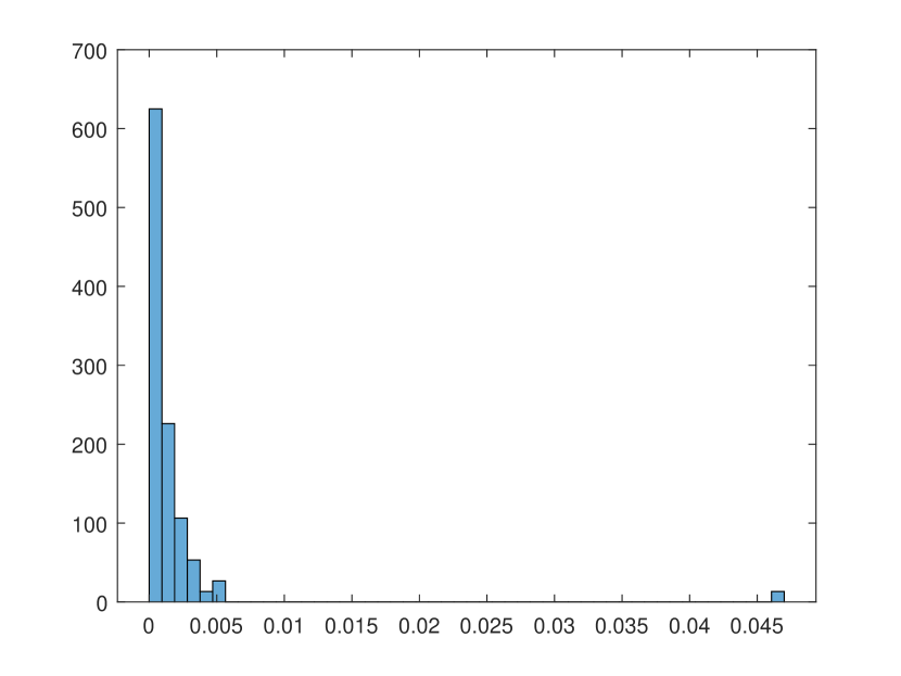
(a) PCA: Cyclical stock returns.

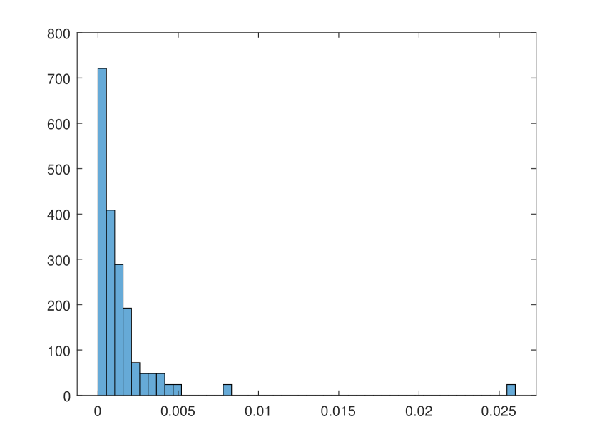
(b) PCA: Non-cyclical stock returns.

Figure 10. Eigenvalues from PCA for cyclical and non-cyclical groups of stock returns.

References

- Ahn and Horenstein [2013] S. C. Ahn and A. R. Horenstein. Eigenvalue ratio test for the number of factors. Econometrica, 81(3):1203–1227, 2013.
- Anderson [1999] T. W. Anderson. Asymptotic theory for canonical correlation analysis. Journal of Multivariate Analysis, 70(1):1–29, 1999.
- Anderson [2003] T. W. Anderson. Introduction to multivariate statistical analysis, 3rd edition. John Wiley & Sons, 2003.
- Andreou et al. [2019] E. Andreou, P. Gagliardini, E. Ghysels, and M. Rubin. Inference in group factor models with an application to mixed-frequency data. Econometrica, 87(4):1267–1305, 2019.
- Bai and Ng [2002] J. Bai and S. Ng. Determining the number of factors in approximate factor models. Econometrica, 70(1):191–221, 2002.
- Bai and Ng [2007] J. Bai and S. Ng. Determining the number of primitive shocks in factor models. Journal of Business & Economic Statistics, 25(1):52–60, 2007.
- Bai and Ng [2008] J. Bai and S. Ng. Large dimensional factor analysis. Foundations and Trends® in Econometrics, 3(2):89–163, 2008.
- Baik and Silverstein [2006] J. Baik and J. W. Silverstein. Eigenvalues of large sample covariance matrices of spiked population models. Journal of multivariate analysis, 97(6):1382–1408, 2006.
- Baik et al. [2005] J. Baik, G. Ben Arous, and S. Péché. Phase transition of the largest eigenvalue for nonnull complex sample covariance matrices. Annals of Probability, pages 1643–1697, 2005.
- Bao and Wang [2022] Z. Bao and D. Wang. Eigenvector distribution in the critical regime of BBP transition. Probability Theory and Related Fields, 182(1-2):399–479, 2022.
- Bao et al. [2019] Z. Bao, J. Hu, G. Pan, and W. Zhou. Canonical correlation coefficients of high-dimensional gaussian vectors: Finite rank case. Annals of Statistics, 47(1):612–640, 2019.
- Benaych-Georges and Nadakuditi [2011] F. Benaych-Georges and R. R. Nadakuditi. The eigenvalues and eigenvectors of finite, low rank perturbations of large random matrices. Advances in Mathematics, 227(1):494–521, 2011.
- Benaych-Georges and Nadakuditi [2012] F. Benaych-Georges and R. R. Nadakuditi. The singular values and vectors of low rank perturbations of large rectangular random matrices. Journal of Multivariate Analysis, 111:120–135, 2012.
- Bhatia [1997] R. Bhatia. Matrix analysis. Springer, 1997.
- Bloemendal et al. [2016] A. Bloemendal, A. Knowles, H.-T. Yau, and J. Yin. On the principal components of sample covariance matrices. Probability theory and related fields, 164(1-2):459–552, 2016.
- Bouchaud et al. [2007] J.-P. Bouchaud, L. Laloux, M. A. Miceli, and M. Potters. Large dimension forecasting models and random singular value spectra. The European Physical Journal B, 55:201–207, 2007.
- Breitung and Pigorsch [2013] J. Breitung and U. Pigorsch. A canonical correlation approach for selecting the number of dynamic factors. Oxford Bulletin of Economics and Statistics, 75(1):23–36, 2013.
- Bykhovskaya and Gorin [2022a] A. Bykhovskaya and V. Gorin. Cointegration in large VARs. Annals of Statistics, 50(3):1593–1617, 2022a.
- Bykhovskaya and Gorin [2022b] A. Bykhovskaya and V. Gorin. Asymptotics of cointegration tests for high-dimensional VAR(). Working Paper, 2022b.
- Choi et al. [2021] I. Choi, R. Lin, and Y. Shin. Canonical correlation-based model selection for the multilevel factors. Journal of Econometrics, 2021.
- Constantine [1963] A. G. Constantine. Some non-central distribution problems in multivariate analysis. The Annals of Mathematical Statistics, 34(4):1270–1285, 1963.
- Cunha et al. [2010] F. Cunha, J. J. Heckman, and S. M. Schennach. Estimating the technology of cognitive and noncognitive skill formation. Econometrica, 78(3):883–931, 2010.
- Fama and French [1992] E. F. Fama and K. R. French. The cross-section of expected stock returns. the Journal of Finance, 47(2):427–465, 1992.
- Fan et al. [2011] J. Fan, J. Lv, and L. Qi. Sparse high-dimensional models in economics. Annual Review of Economics, 3(1):291–317, 2011.
- Fan et al. [2016] J. Fan, Y. Liao, and H. Liu. An overview of the estimation of large covariance and precision matrices. The Econometrics Journal, 19(1):C1–C32, 2016.
- Gavish et al. [2022] M. Gavish, W. Leeb, and E. Romanov. Matrix denoising with partial noise statistics: Optimal singular value shrinkage of spiked F-matrices. arXiv preprint arXiv:2211.00986, 2022.
- Gittins [1985] R. Gittins. Canonical Analysis: A Review with Applications in Ecology. Springer, 1985.
- Hallin and Liska [2007] M. Hallin and R. Liska. Determining the number of factors in the general dynamic factor model. Journal of the American Statistical Association, 102(478):603–617, 2007.
- Hotelling [1936] H. Hotelling. Relations between two sets of variates. Biometrika, 28(3/4):321–377, 1936.
- Hsu [1939] P. Hsu. On the distribution of roots of certain determinantal equations. Annals of Eugenics, 9(3):250–258, 1939.
- Hsu [1941] P. Hsu. On the limiting distribution of the canonical correlations. Biometrika, 32(1):38–45, 1941.
- Johansen [1988] S. Johansen. Statistical analysis of cointegrating vectors. Journal of Economic Dynamics and Control, 12(2–3):231–254, 1988.
- Johnstone [2001] I. M. Johnstone. On the distribution of the largest eigenvalue in principal components analysis. Annals of Statistics, 29(2):295–327, 2001.
- Johnstone [2008] I. M. Johnstone. Multivariate analysis and Jacobi ensembles: largest eigenvalue, Tracy-widom limits and rates of convergence. Annals of Statistics, 36(6):2638–2716, 2008.
- Johnstone and Lu [2009] I. M. Johnstone and A. Y. Lu. On consistency and sparsity for principal components analysis in high dimensions. Journal of the American Statistical Association, 104(486):682–693, 2009.
- Johnstone and Onatski [2020] I. M. Johnstone and A. Onatski. Testing in high-dimensional spiked models. The Annals of Statistics, 48(3), 2020.
- McCracken and Ng [2016] M. W. McCracken and S. Ng. FRED-MD: A monthly database for macroeconomic research. Journal of Business & Economic Statistics, 34(4):574–589, 2016.
- Muirhead [2009] R. J. Muirhead. Aspects of multivariate statistical theory. John Wiley & Sons, 2009.
- Muirhead and Waternaux [1980] R. J. Muirhead and C. M. Waternaux. Asymptotic distributions in canonical correlation analysis and other multivariate procedures for nonnormal populations. Biometrika, 67(1):31–43, 1980.
- Nadler [2008] B. Nadler. Finite sample approximation results for principal component analysis: A matrix perturbation approach. Annals of Statistics, pages 2791–2817, 2008.
- Onatski [2009] A. Onatski. Testing hypotheses about the number of factors in large factor models. Econometrica, 77(5):1447–1479, 2009.
- Onatski [2012] A. Onatski. Asymptotics of the principal components estimator of large factor models with weakly influential factors. Journal of Econometrics, 168(2):244–258, 2012.
- Onatski and Wang [2018] A. Onatski and C. Wang. Alternative asymptotics for cointegration tests in large VARs. Econometrica, 86(4):1465–1478, 2018.
- Onatski and Wang [2019] A. Onatski and C. Wang. Extreme canonical correlations and high-dimensional cointegration analysis. Journal of Econometrics, 212(1):307–322, 2019.
- Onatski et al. [2013] A. Onatski, M. M. Moreira, and M. Hallin. Asymptotic power of sphericity tests for high-dimensional data. Annals of Statistics, 41(3):1204–1231, 2013.
- Papageorge and Thom [2020] N. W. Papageorge and K. Thom. Genes, education, and labor market outcomes: evidence from the health and retirement study. Journal of the European Economic Association, 18(3):1351–1399, 2020.
- Paul [2007] D. Paul. Asymptotics of sample eigenstructure for a large dimensional spiked covariance model. Statistica Sinica, pages 1617–1642, 2007.
- Potters and Bouchaud [2020] M. Potters and J.-P. Bouchaud. A First Course in Random Matrix Theory: For Physicists, Engineers and Data Scientists. Cambridge University Press, 2020.
- Simon [1998] T. P. Simon. Assessing the Sustainability and Biological Integrity of Water Resources Using Fish Communities. CRC Press, 1998.
- Stock and Watson [2011] J. H. Stock and M. W. Watson. Dynamic factor models. Oxford Handbooks Online, 2011.
- Thompson [1984] B. Thompson. Canonical correlation analysis: Uses and interpretation. Number 47. Sage, 1984.
- Wachter [1980] K. W. Wachter. The limiting empirical measure of multiple discriminant ratios. Annals of Statistics, pages 937–957, 1980.
- Wang et al. [2020] H.-T. Wang, J. Smallwood, J. Mourao-Miranda, C. H. Xia, T. D. Satterthwaite, D. S. Bassett, and D. Bzdok. Finding the needle in a high-dimensional haystack: Canonical correlation analysis for neuroscientists. NeuroImage, 216:116745, 2020.
- Witten and Tibshirani [2009] D. M. Witten and R. J. Tibshirani. Extensions of sparse canonical correlation analysis with applications to genomic data. Statistical applications in genetics and molecular biology, 8(1), 2009.
- Yang [2022a] F. Yang. Sample canonical correlation coefficients of high-dimensional random vectors: Local law and Tracy-Widom limit. Random Matrices: Theory and Applications, 11(1):2250007, 2022a.
- Yang [2022b] F. Yang. Limiting distribution of the sample canonical correlation coefficients of high-dimensional random vectors. Electronic Journal of Probability, 27:1–71, 2022b.
- Zhuang et al. [2020] X. Zhuang, Z. Yang, and D. Cordes. A technical review of canonical correlation analysis for neuroscience applications. Human Brain Mapping, 41(13):3807–3833, 2020.