Accelerating Sampling and Aggregation Operations in GNN Frameworks with GPU Initiated Direct Storage Accesses

Abstract.

Graph Neural Networks (GNNs) are emerging as a powerful tool for learning from graph-structured data and performing sophisticated inference tasks in various application domains. Although GNNs have been shown to be effective on modest-sized graphs, training them on large-scale graphs remains a significant challenge due to lack of efficient data access and data movement methods. Existing frameworks for training GNNs use CPUs for graph sampling and feature aggregation, while the training and updating of model weights are executed on GPUs. However, our in-depth profiling shows the CPUs cannot achieve the throughput required to saturate GNN model training throughput, causing gross under-utilization of expensive GPU resources. Furthermore, when the graph and its embeddings do not fit in the CPU memory, the overhead introduced by the operating system, say for handling page-faults, comes in the critical path of execution.

To address these issues, we propose the GPU Initiated Direct Storage Access (GIDS) dataloader, to enable GPU-oriented GNN training for large-scale graphs while efficiently utilizing all hardware resources, such as CPU memory, storage, and GPU memory with a hybrid data placement strategy. By enabling GPU threads to fetch feature vectors directly from storage, GIDS dataloader solves the memory capacity problem for GPU-oriented GNN training. Moreover, GIDS dataloader leverages GPU parallelism to tolerate storage latency and eliminates expensive page-fault overhead. Doing so enables us to design novel optimizations for exploiting locality and increasing effective bandwidth for GNN training. Our evaluation using a single GPU on terabyte-scale GNN datasets shows that GIDS dataloader accelerates the overall DGL GNN training pipeline by up to 392$\times$ when compared to the current, state-of-the-art DGL dataloader.

1. Introduction

Owing to their expressive power, Graph Neural Networks (GNNs) effectively capture the rich relational information embedded among input nodes and edges, leading to improved generalization performance over traditional machine learning techniques. As a result, GNNs have gained significant attention in recent years, due to their efficacy in various graph-based machine learning applications, such as node classification (Kipf and Welling, 2017; Hamilton et al., 2017; Veličković et al., 2018; Ramezani et al., 2020), recommendation (Fan et al., 2019; Pal et al., 2020), fraud detection (Liu et al., 2020; Wang et al., 2019; Wu et al., 2023; Ye et al., 2021), and link prediction (Zhang and Chen, 2018; Garcia and Bruna, 2018; Rossi et al., 2022).

To cater to this growing interest, new open-source frameworks such as PyTorch Geometric (PyG) (Fey and Lenssen, 2019), Spektral (Grattarola and Alippi, 2021), and Deep Graph Library (DGL) (Zheng et al., 2021) have been developed to provide optimized operators required by GNNs, such as message-passing for aggregating feature information across related graph nodes, and graph-specific neural network computation layers. Although GNN frameworks leverage GPUs for highly parallelized matrix computations, GNN training faces challenges beyond computation efficiency. While limited GPU memory capacity can be partially addressed with mini-batching and sampling for small to medium scale graph datasets, larger graphs do not fit into the GPU memory when it comes to graph sampling and feature aggregation. To address this problem, frameworks like DGL exploit Unified Virtual Addressing (UVA), pinning the graph dataset, including both the graph structure data and feature data, into the CPU memory to enable efficient subgraph extraction and feature aggregation using GPU kernels with zero-data copy transfer (Min et al., 2021).

For large-scale graphs that do not fit into the CPU memory, the UVA approach is no longer sufficient. There are several solutions to support large-scale GNN training: (a) multi-node/multi-GPU, (b) tiling, and (c) memory-mapped file. Leveraging multiple nodes or GPUs (Cai et al., 2023; Wang et al., 2022; Jia et al., 2020; Ma et al., 2019; Balin et al., 2023) to partition the graph across the nodes to support large-scale GNN training is an expensive approach (Zhao et al., 2015). Tiling (Hu et al., 2020; Zhang et al., 2021a) can be used to support large-scale GNN training by leveraging graph partitioning to load tiled data and transfer it to the GPU. This approach shows poor performance due to the random access pattern and the additional cost for pre-processing the input data. Finally, the most convenient solution to train large-scale graph datasets on a single GPU is exploiting the memory-mapped file technique, which maps the graph data stored on disk to virtual memory, enabling access to the data without first loading the entire dataset into memory. Previous studies (Park et al., 2022; Zhu et al., 2019; Lin et al., 2020; Rajbhandari et al., 2021) extended the memory-mapped files approach and leveraged the in-memory caching mechanism to mitigate the storage overhead.

Despite its conceptual simplicity, the use of memory-mapped files in GNN training faces performance challenges due to the heavy software overhead in handling page faults and its inability to tolerate long latency incurred during data retrieval from storage. The storage latency, which is two to three orders of magnitude longer than the DRAM access latency, becomes a bottleneck in the GNN training process due to sparse and irregular graph data access patterns and the inability of the memory-mapped file approach to overlap the latencies of these accesses, resulting in poor overall performance. In Section 2.3, we show that when using memory-mapped files, the sampling and feature aggregation stages of the GNN training pipeline dominate the overall execution time and severely limit the overall GNN training performance.

In this paper, we propose a new approach called GPU Initiated Direct Storage Access (GIDS) dataloader to tackle the challenges of GNN training on large-scale graphs by enabling fully GPU-oriented GNN training. We extend the key idea of BaM system (Qureshi et al., 2023), which leverages GPU parallelism to hide storage latency, to address the memory capacity problem for GPU-accelerated GNN training.

We further propose a three-part hybrid strategy for the GIDS dataloader to efficiently utilize all hardware resources (CPU memory, storage, and GPU memory) to accelerate the GNN training process for large-scale graphs. First, GIDS dataloader stores the feature data of the graph in storage as the feature data typically accounts for the vast majority of the total graph dataset size for large-scale graphs (see Table 4 for examples). GIDS dataloader overcomes the long storage access latency by allowing GPU threads to directly fetch feature data, leveraging the massive GPU thread-level parallelism to overlap the latencies of many storage accesses. This direct access avoids CPU software bottlenecks, leading to full utilization of storage throughput. Second, GIDS pins the graph structure data, whose size is typically tiny compared to the feature data, in the CPU memory to enable GPU graph sampling via UVA zero-data copy transfer. Finally, GIDS dataloader allocates GPU memory for the GPU software-defined cache to store feature data for recently accessed nodes to minimize the storage accesses. Moreover, we designed window buffering technique to further improve GPU cache utilization.

We evaluate the effectiveness of our work by demonstrating its implementation with NVMe SSDs in the DGL framework. Our experiments show that GIDS accelerates the feature aggregation process by up to 160$\times$ and the graph sampling by 25$\times$ compared to the state-of-the art DGL dataloader that uses the memory-mapping approach with only a single SSD. When scaled to four SSDs, the performance advantage of the GIDS dataloader increases to 627$\times$ for aggregation.

Moreover, with four SSDs connected, the GIDS dataloader outperforms the state-of-the-art DGL dataloader that uses the UVA-based approach for modest-size graphs, which stores entire graph datasets in the CPU memory. GIDS dataloader achieves this by increasing the collective SSD bandwidth to saturate the PCIe Gen4 bandwidth of the GPU and amplifying the effective bandwidth with GPU software-defined cache. With GIDS and multiple SSDs, even the modest-sized graphs can simply be stored in SSDs and no longer need to take up space in the CPU memory.

We make the following key contributions in this paper.

• We analyze the limitations of the existing GNN frameworks while executing large graph datasets and show that the existing CPU-initiated approach cannot keep up with the demands of GPU-accelerated GNN training.

• We introduce a novel GPU-oriented GNN dataloader that enables direct storage accesses for GPU threads to enable and accelerate large-scale GNN training.

• We present an effective data placement strategy to efficiently leverage all available hardware resources: CPU memory, storage, and GPU memory for large-scale GNN training.

• We propose novel optimizations to improve GPU software-cache efficiency by exploiting locality in GNN training.

We demonstrate GIDS dataloader’s effectiveness and flexibility by measuring performance using billion-scale datasets that do not fit in the CPU memory. The results based on the NVIDIA A100 GPUs and 512GB CPU memory capacity show that GIDS dataloader achieves up to 627$\times$ speedup in data aggregation and 392$\times$ speedup in overall training over a state-of-the-art GNN dataloader.

2. Background

In this section, we provide an overview of GNN models, followed by an introduction to mini-batching and sampling-based GNN training. We then explain the state-of-the-art framework for large-scale GNN training and its challenges.

2.1. Graph Neural Networks (GNNs)

Graph Neural Networks (GNNs) have recently gained prominence in solving machine learning problems by incorporating graph structure information (Kipf and Welling, 2017; Veličković et al., 2018; Defferrard et al., 2016; Bruna et al., 2014). These networks typically consist of multiple layers and operate through layer-wise message passing.

Given a graph $\mathcal{G}(\mathcal{V},\mathcal{E})$, with vertex set $\mathcal{V}$ and edge set $\mathcal{E}$, the node feature vectors for each vertex $v\in\mathcal{V}$ are represented as $x_{v}$. The node embedding of vertex $v$ at layer $l$ is denoted as $h_{v}^{(l)}$, with $h_{v}^{(0)}$ initialized with the node feature vector. The GNN updates the node embeddings using the equation:

(1) $$h_{v}^{(l+1)}=f(h_{v}^{(l)},{h_{w}^{(l)}}_{w\in\mathcal{N}(v)}),$$

where $\mathcal{N}(v)$ defines the neighborhood set of $v$, $h_{w}^{(l)}$ denotes the node embbeding of the neghibor node $w$ at layer $l$, and $f$ is a parameterized update function.

Graph data consists of two components: graph structure data and node feature data. The graph structure data represents the edges and nodes of the graph, while the node feature data represents the feature embeddings for each node. Sparse matrix formats such as Coordinate (COO) format and Compressed Sparse Column (CSC) format are commonly used to store the graph structure data, whereas the node features are typically stored in an $N\times D$ matrix, where $N$ is the total number of nodes in the graph, and $D$ is the dimension of each node feature. The size of each node’s feature can vary greatly but typically ranges from 512B to 4KB. For large-scale graphs with billions of nodes, the size of the node feature data can reach several tens of terabytes. As a result, managing the node feature data for large-scale GNN training with limited memory capacity is a challenging task.

2.2. GNN Training Pipeline

GNN training on large graph datasets involves mainly four stages: graph sampling, feature aggregation, data transfer, and model training. Mini-batch training is commonly used in these models for scalability and computational efficiency (Keskar et al., 2017; Wilson and Martinez, 2003; Preprint et al., 2021). In this section, we briefly describe the mini-batching technique and each key stage of the GNN training pipeline.

2.2.1. Mini-batching

Mini-batching of GNN models involves splitting the graph into smaller sub-graphs and training the network on each of these sub-graphs. During each iteration of the training process, a batch of sub-graphs is loaded into GPU memory for computation. The batch size must be carefully chosen to prevent GPU memory overflow during training. Mini-batching also exposes more parallelism to the GPU training kernel, which significantly improves training speed and efficiency and makes it a popular approach for many GNN models. Previous studies have demonstrated that training neural networks with mini-batches can also lead to faster convergence and better optimization compared to training on the entire dataset (Keskar et al., 2017; Wilson and Martinez, 2003; Preprint et al., 2021).

2.2.2. Node Sampling

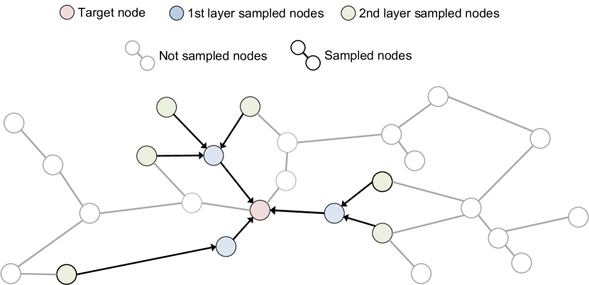
Figure 1. A subgraph generated by a uniformly random selection method for two-layer Neighborhood Sampling.

Mini-batching alone cannot fully address the scalability limitations when working with large graphs. Even with small batch sizes, the training cost can still be substantial due to the exponential growth of memory footprint when collecting k-hop neighbors. GraphSAGE (Hamilton et al., 2017) introduced the concept of neighborhood sampling to tackle this problem. GraphSAGE reduces the computation and memory footprint by randomly sampling a fixed number of neighboring nodes rather than including all nodes in the graph. To ensure a sufficient level of randomness in the training process, GraphSAGE uses a uniformly random selection method for neighborhood sampling. Figure  1 illustrates an example of neighborhood sampling with a 2-hop computational graph. In this example, the sampling size is set to 3, meaning up to three neighboring nodes of the target node are selected. With two layers, the total mini-batch size is 11 (1 + 3 + 7).

2.2.3. Node Feature Aggregation and Transfer

The features for each sampled node in the mini-batch must be gathered before the training on the mini-batch can start. In cases where node feature data is too large to fit into CPU memory, the current state-of-the-art approach (Zheng et al., 2021; Khatua et al., 2023) first transfers the features of the sampled nodes from storage to the CPU memory, and then from the CPU memory to the GPU memory via the PCIe interconnect. Afterward, the GPU model training kernels can consume the fetched node features.

2.3. Limitation of Existing GNN Frameworks

State-of-the-art GNN frameworks, such as DGL (Zheng et al., 2021) and PyG (Fey and Lenssen, 2019), have significantly improved GNN training performance by utilizing a hybrid CPU-GPU training system, where the CPU is responsible for data preparation, and the GPU handles the model training. To increase the effective memory capacity, DGL introduced the UVA-based GNN training technique (Min et al., 2021), which pins the entire graph dataset (both graph and feature vectors) in the CPU memory and transfers data from the CPU to the GPU through zero-copy accesses, enabling the GPU to execute graph sampling and feature aggregation. While this approach helps to scale to larger graph datasets whose sizes exceed the GPU memory capacity, it cannot handle large-scale graphs whose sizes surpasses the capacity of the CPU memory since all graph data must be pinned in the CPU memory for the UVA-based technique to work.

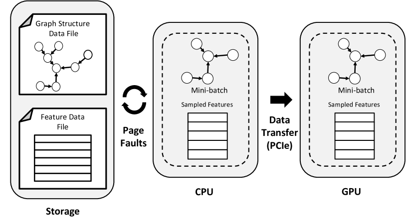
Figure 2. Illustration of the GNN training process with the memory-mapping DGL dataloader

The existing GNN frameworks rely on the CPU for graph sampling and feature aggregation execution to support graph datasets that cannot fit into the CPU memory. The key idea is to provide a notion of infinite virtual memory by memory-mapping the node feature vector files into the CPU virtual address space and allow the CPU to page fault when the requested feature vector is unavailable in the CPU memory. This eliminates the need for loading the entire dataset into the CPU memory and employs the operating system (OS) page fault handler to bring parts of the graph data stored in the disk to the application’s address space in an on-demand manner. Figure 2 illustrates the GNN training process using the approach of the memory-mapped file in the DGL framework. During the node feature aggregation stage, the CPU accesses the node features mapped in its virtual memory space, and the OS page fault handler brings the pages that contain the accessed features from storage into the CPU memory when it misses from the OS page cache.

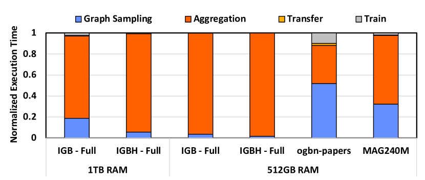
Figure 3. GNN training time breakdown for the baseline DGL dataloader for different graph datasets. The node feature data is accessed from memory-mapped files, while the graph structure data is stored in the CPU memory. The GraphSAGE model is used as the GNN training model. The graph properties are listed in Table 2.

Unfortunately, implementing node feature aggregation using a memory-mapped approach makes the node feature aggregation by far the main bottleneck of the overall training pipeline. Our profiling of each stage in the GNN training execution shows the iteration time is clearly dominated by the sampling and node aggregation stages, as shown in Figure 3. For example, the training stage is barely visible for the IGB-Full and IGBH-Full graphs, the largest two graphs used in our evaluations. This is because, for large-scale graphs, the additional cost of page faults exacerbates the gap between the data preparation throughput and model training throughput. Thus, the key to improving the GNN training performance while training on large graphs is to drastically accelerate the sampling and feature aggregation stages (i.e., the data preparation stages).

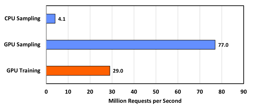
Figure 4. Request generation rate of data preparation on CPU and GPU, and request consumption rate on GPU on IGB-small dataset. The CPU and GPU used in this measurement are listed in Table 1.

Previous research (Lin et al., 2020; Zhu et al., 2019; Park et al., 2022; Wang et al., 2023) has aimed to enhance the efficiency of node aggregation and sampling stages by using specific in-memory caching mechanisms to minimize redundant storage accesses and/or utilizing pipelining techniques to conceal graph sampling time. However, for these methods to be effective, the CPU-driven request initiation mechanism must generate requests at a sufficiently high rate to hide long storage access latency and prevent the GPU from waiting for data. In GNN training, the storage access requests are for feature vectors that must be aggregated before training can begin. To this end, we first investigate whether CPUs can generate requests at a sufficiently high rate during the sampling stage of GNN training iterations. To answer this question, we use the baseline DGL dataloader that loads the entire graph into the CPU memory, pins it, and utilizes CPU threads to perform the node sampling operation.

Figure 4 shows the request generation and consumption rate of CPU and GPU for the two data preparation stages of the GNN training pipeline: sampling and training. After the node feature vectors are loaded into the GPU memory, the GPU-accelerated training kernels can consume them at a rate greater than 29 million requests per second. This implies to maximize effective GPU utilization and minimize GNN training time for large graphs, the effective request generation rate must match or exceed the consumption rate. However, using the CPU-driven request generation sampling stage, the CPU cannot generate more than 4.1 million feature vector requests per second, even when using multiple threads (16 in this experiment beyond which the rate plateaus). This is because the sampling computation involves repeatedly traversing the graph and accessing its edges and nodes, making it difficult for the CPU to keep up with the consumption rate of the GPU-accelerated training kernels. In contrast, the GPU can generate more than 77 million feature requests per second in the sampling stage, which is significantly higher than the consumption rate required by the training kernels.

Based on these two key insights, our proposed GIDS dataloader offloads the data preparation stages to the GPU to benefit from its faster request generation rate. We further adopt the recent technique of BaM (Qureshi et al., 2023) which enables direct storage device access by the GPU, eliminating the overhead of OS page faults during feature vector data access.

2.4. The BaM System

The BaM system (Qureshi et al., 2023) aims to tackle the problem of storage latency in big data GPU applications. The key idea behind BaM is to allow GPU threads to have direct access to the storage, making use of the massive data-level parallelism that GPUs provide. As a massive number of GPU threads can initiate direct storage access without incurring CPU-GPU synchronization or CPU software overhead, the GPU can take full advantage of parallelism to hide long storage access latency, enabling it to achieve peak storage bandwidth.

By exploiting inexpensive dense storage, the GPU can drastically expand its memory capacity, which is extremely useful for applications that require computation-directed sparse access to massive datasets, such as GNN training.

3. System Design

To address the challenges associated with state-of-the-art large-scale GNN training, we design and implement the GIDS dataloader, which enables fully GPU-oriented GNN training for large graphs. This section describes the design of GIDS dataloader. First, we provide an overview of design goals and introduce a new dataloader for sampling-based GNN models, extended from the DGL dataloader. We then describe our optimizations to further improve the performance.

3.1. Data Placement Strategy and GNN Workflow

The GIDS dataloader is designed to improve the performance and scalability of GNNs by exploiting the GPU’s parallelism to accelerate data preparation. As discussed in Section 2.3, the workflow of the CPU-oriented GNN training fails to generate requests at a sufficient rate to match the GPU training throughput, thus limiting the overall GNN training performance.

To address this deficiency in generating requests, the GIDS dataloader moves the data preparation process from the CPU to the GPU. As shown in Figure 3, the request generation rate of the sampling and aggregation stages running on the GPU exceeds the GPU training throughput. The next major bottleneck is the insufficient storage access throughput.

We tackle the storage access bottleneck by leveraging the BaM system (Qureshi et al., 2023) to allow GPU threads to directly access the storage, thus avoiding the CPU page-fault handling software overhead. The BaM system is integrated into our GIDS DGL dataloader with an interface that manages the metadata and the buffer pointers for the output mini-batch tensors. Instead of actually loading the data, we set up the mappings so that each access is translated into a BaM cache access which either finds the data in cache or generates a storage access request through the BaM cache miss handler.

Although BaM solves the CPU software overhead problem and fully hides storage latency by exploiting GPU data level parallelism, the available I/O bandwidth alone is still not enough to match the GPU training throughput. Thus, efficiently utilizing all available resources to further improve the data preparation process is key to achieving high-performance GNN training.

To achieve this goal, the GIDS dataloader utilizes a hybrid data management strategy that efficiently uses three hardware resources: the CPU memory, the GPU device memory, and the storage devices, based on the data access pattern and the access granularity. First, GPU memory is used as a software-defined cache to reduce redundant storage accesses and utilize the high bandwidth of the GPU memory. Under the hybrid data management strategy, data used by more irregular and smaller access granularity patterns are stored in the CPU memory, while data accessed through larger granularity is backed by storage. This is because that low data granularity access pattern increases I/O amplification, resulting in lower effective bandwidth. Also, irregular data access patterns can pollute the software-defined GPU cache.

Based on this data management strategy, the GIDS dataloader stores the node feature data in the storage while the graph structure data is pinned in the CPU memory since the graph structure data (4-8B) accessed by the sampling process has a much finer granularity access pattern than the node feature data (512-4096B) that is accessed by the aggregation process. Although graph structure data is pinned in the memory, this does not result in any memory capacity issues because graph structure data accounts for as little as 5% of the total dataset size and the structure data fits comfortably in the CPU memory even for terabyte-scale graphs. (see Table 4).

Finally, the GIDS dataloader uses the GPU device memory as a software-defined cache to temporarily store the feature data of recently accessed nodes, reducing the number of storage accesses and improving feature aggregation performance. This is achieved by configuring the BaM software-defined cache and setting up a custom cache-line replacement policy. The utilization of the GPU software-defined cache is further optimized through GIDS-specific cache optimizations, such as window buffering.

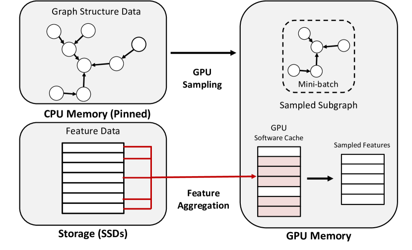
Figure 5. Illustration of the GNN training process with GIDS dataloader

Figure 5 illustrates the workflow of the GIDS dataloader based on this data placement strategy. The process begins with neighborhood sampling to generate a mini-batch with sampled nodes. Since the graph structure data is pinned in the CPU memory and this step is executed on the GPU, the GPU threads access it via zero-copy data transfer (Min et al., 2021). The sampled sub-graphs are kept in the GPU memory. Once the sampling process is complete, GPU threads check the software cache in the GPU memory to determine if the feature data for the sampled nodes is stored in the cache. If not, they directly access the storage to fetch the data and store it in the cache for future use. After fetching all the feature data for the sampled nodes in the mini-batch, the GPU executes the training process and then updates the learning parameters for the model.

3.2. Tolerating Storage Latency during Feature Aggregation

The GIDS dataloader takes advantage of the massive thread-level parallelism provided by GPUs to effectively handle storage latency during feature aggregation. To this end, it is essential to have a sufficient number of concurrent storage access requests during the feature aggregation stage to maximize storage throughput.

Based on the reported results from BaM (Qureshi et al., 2023), a single PCIe Gen4 server-grade SSD’s read peak throughput can be achieved with 32,768 concurrent storage access requests. When the cache-line size is the same as the node embedding feature size, the number of storage accesses during feature aggregation is equivalent to the number of sampled nodes in the mini-batch. Therefore, the size of a mini-batch should be larger than 32,768 nodes to achieve peak SSD throughput.

The size of the mini-batch can be adjusted based on the computational resources and specific requirements of the task. However, for large-scale graph datasets that contain hundreds of millions to a billion nodes, the typical size of a mini-batch is between 1,024 to 4,096 subgraphs (Zhang et al., 2020). Since the size of a subgraph for a large-scale graph can easily exceed 50 sampled nodes, the number of sampled nodes in a single mini-batch easily exceeds 200K nodes. Thus, the requirement of having at least 32,768 storage access requests during feature aggregation does not limit the flexibility of the GNN models.

Another critical factor that determines the mini-batch size is the GPU device memory capacity. The mini-batch size must be smaller than the available GPU device memory as the mini-batch is transferred from CPU to GPU for model training. Practically, there should be enough GPU device memory space after allocating space for a mini-batch since GPU device memory is also utilized for training and other data structures.

For a cache-line size of 4KB and 32,768 storage access requests, the mini-batch size is  0.125 GB with the meta-data and a few Megabytes for model parameters. The NVIDIA A100 offers up to 80 GB of GPU memory, providing enough space for a mini-batch and model parameters. Thus, GPU memory capacity is not a limiting factor for the mini-batch size.

3.3. GPU Software-defined Cache for Efficient Feature Aggregation

Although GIDS dataloader can effectively handle storage latency and achieve peak storage bandwidth during feature aggregation, the achievable storage read bandwidth is orders of magnitude lower than the GPU memory bandwidth as High Bandwidth Memory 2 (HBM2) of the recent NVIDIA GPUs, can provide  2TB/s bandwidth (HBM, 2023) whereas the storage read bandwidth is limited by the 32GB/s PCIe in-take bandwidth of A100. Therefore, efficient utilization of GPU memory is necessary to amplify the effective bandwidth and further accelerate the feature aggregation process.

To address this, the GIDS dataloader employs the GPU software-defined cache. Unlike the GPU hardware caches, which helps to conserve DRAM bandwidth, the GIDS software-defined cache is used to help conserve storage bandwidth. The GPU software-defined cache in GIDS dataloader temporarily stores the feature data of recently accessed nodes, reducing the need for frequent storage accesses. During initialization, the GPU software-defined cache is allocated a fixed-size space with a configurable cache-line size. For each storage access, the entire cache-line is fetched from storage and stored in the GPU cache. Thus, to avoid I/O amplification, the GIDS dataloader sets the cache-line size equal to or slightly larger than the node feature embedding size. The GPU software-defined cache also tracks the status of each cache-line, enabling the system to determine whether the cache-line is in the cache, in use by another thread, or available for eviction.

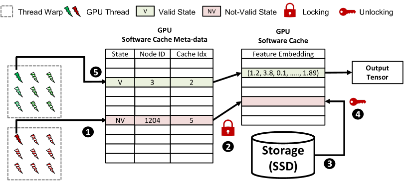
Figure 6. Example of GIDS GPU software-defined cache update process

Figure 6 illustrates the process of accessing storage for node feature vectors through the GPU software-defined cache. When a thread attempts to access the cache, it checks the state of the corresponding cache-line from the meta-data. If the cache-line is not found in the cache ( ) the thread locks the cache-line ( ), selects a cache-line to evict, and requests the cache-line from storage ( ). Upon completion of the request, the thread marks the cache-line state as valid and unlocks the cache-line ( ). This allows threads to fetch data directly from the GPU cache when the cache-line is in a valid state ( ), avoiding unnecessary I/O traffic. Additionally, each thread warp is assigned to access the feature embedding of the same node, reducing contention and coalescing memory accesses.

3.4. Window Buffering Cache Optimization

When the graph dataset is much larger than the GPU cache, achieving high reusability of node feature data becomes challenging due to the random nature of the neighborhood sampling process. In such scenarios, GPU memory space becomes a valuable resource, and maximizing its utilization is crucial.

One effective method to increase GPU cache utilization is to provide the cache with information about the dataset, which can involve pinning, i.e. marking certain sections of node features as highly reusable to reduce the likelihood of cache-lines in these sections being evicted  (Min et al., 2022; Lin et al., 2020). However, this approach presents a significant challenge in the context of GNN feature aggregation. This is because the nodes to be reused in the next iteration are randomly selected, making it challenging to mark them before launching the kernel.

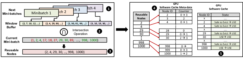
Figure 7. Example of window buffering technique from GIDS dataloader

To overcome this challenge, the GIDS dataloader introduces a novel technique called window buffering. Unlike the traditional frameworks, GIDS leverages the BaM software-defined cache which supports the customization of cache-line eviction policies. The window buffering technique reduces cache thrashing by avoiding the eviction of reusable node feature vectors through mini-batch look-ahead. This is achieved by conducting a graph sampling operation for a configurable number of iterations to fill the window buffer with sampled node IDs and avoiding the eviction of feature vectors for reused nodes in the window buffer. Therefore, the dataloader can look-ahead to the list of the sampled nodes for the next iterations.

Specifically, as illustrated in Figure 7, the window buffer in GIDS dataloader is initially filled with the node IDs that will be sampled in the next few iterations ( ). Once the window buffer is filled, the sampled node IDs in the current mini-batch are compared with the nodes in the window buffer ( ). Then, the list of nodes that will be reused in the next iterations and the number of occurrences is generated ( ). This information is then used to update the GPU software-defined cache meta-data, which tracks the number of reuses in the next iterations for each node ( ).

During the update stage, when the reuse counter value is shifted from 0 to any positive number, the state of the node in the GPU cache is changed from the “Safe to Evict” state to the "USE" state so that the corresponding cache-line will not be evicted. If the counter value is already a positive number, the state is kept marked as the "USE" state ( ). The counter value is decreased each time the node is reused during the cache-line release stage. When the counter value is set back to 0, the state of the corresponding cache-line is then set back to the “Safe to Evict” state so that other threads can safely evict the cache-line. This approach effectively reduces cache thrashing and improves the performance of GNN feature aggregation on GPUs.

3.5. Leveraging CPU Memory for Graph Sampling

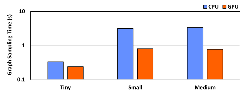
Figure 8. Graph sampling time of CPU and GPU graph sampling on the graphs with different sizes

As shown in Figure 3, the graph sampling throughput is higher on GPU than on CPU despite graph sampling being a sequential process. This is because the graph sampling process is especially latency-critical for large-scale graphs. The fundamental approach to accelerate such a process is to exploit parallelism to hide the latency, which GPUs naturally provide. Figure 8 shows that GPU outperforms CPU for all three datasets, with a performance gain of over 3$\times$ for the medium dataset. However, storing graph structure data in storage incurs multiple problems.

Firstly, the graph sampling process has a smaller data access granularity than the feature aggregation process, resulting in significant I/O amplification. This is because the data accesses to the storage devices are handled in page granularity, such as 4KB, meaning even if only a small segment of data is requested, the entire cache-line is transferred from the storage to GPU memory. Secondly, the random data access pattern from the sampling process makes it challenging for the GPU cache to exploit data locality, which can degrade the performance of the feature aggregation process. This is because the GPU memory is a limited resource, and the random data access pattern can pollute the GPU software-defined cache.

To address these challenges, the GIDS dataloader employs zero-copy data transfer via Unified Virtual Addressing (UVA) for graph structure data. Instead of storing the entire graph data in storage devices, our dataloader allows users to store node feature data on storage while pinning graph structure data in the CPU memory. This makes it possible to execute the graph sampling process on either CPU or GPU. This is a practical approach because the graph structure data is small, even for terabyte-scale graphs that we expect to accommodate in the foreseeable future, as shown in Table 4.

4. Evaluation

4.1. Experimental Setup

Environment. Table 1 summarizes the system configuration for all evaluations. We compare GIDS and the state-of-the-art DGL baseline on an AMD EPYC high-end server-grade system equipped with a NVIDIA A100-40GB GPU and 1TB DDR4 CPU DRAM. 512GB of the CPU memory is locked for evaluation unless otherwise stated. All SSDs used for the evaluations are Intel Optane PCIe Gen4 NVMe SSDs.

Table 1. Configuration used to evaluate GIDS.

Configuration	Specification
CPU	AMD EPYC 7702 64-Core Processor
Memory	1TB DDR4 (512GB is locked)
GPU	NVIDIA A100 HBM2 40GB
	108 SMs, 192KB Shared Memory per SM
	40MB LLC, 1555GBps HBM Bandwidth
S/W	Ubuntu 20.04 LTS, NVIDIA Driver 470.103
	CUDA 11.4
	DGL 0.10
	Pytorch 1.13.0
SSDs	Intel Optane SSDs
	PCIe Gen 4 Interconnect

Datasets. To assess the performance of GIDS dataloader on large-scale graph datasets, we conducted experiments using four real-world datasets: IGB-Full (Khatua et al., 2023), IGBH-Full (Khatua et al., 2023), ogbn-papers100M (Hu et al., 2021), and MAG240M (Wang et al., 2020). Table 2 presents the characteristics of these datasets, such as the number of nodes and edges, the dimension of the node feature data, and the type of graph. It is worth noting that ogbn-papers100M and MAG240M datasets are small enough to fit into the CPU memory of our evaluation system.

For micro-benchmarking with smaller datasets, we used the subgraphs from IGB-Full dataset by following a procedure to maintain consistent characteristics as the original graph. The four graphs are denoted as IGB-tiny, IGB-small, IGB-medium, and IGB-large and their properties are shown in Table 3. The node feature data dimension is 1024, which is the same as IGB-Full dataset.

Table 2. Real-world dataset used for evaluating GIDS.

Dataset	Graph Type	Number of Nodes	Number of Edges	Feature Dimension
ogbn-papers100M	Homogeneous	111,059,956	1,615,685,872	128
IGB-Full	Homogeneous	269,364,174	3,995,777,033	1024
MAG240M	Heterogeneous	244,160,499	1,728,364,232	768
IGBH-Full	Heterogeneous	547,306,935	5,812,005,639	1024

Table 3. IGB datasets used for micro-benchmarks.

Dataset	Graph Type	Number of Nodes	Number of Edges	Feature Dimension
IGB-tiny	Homogeneous	100,000	547,416	1024
IGB-small	Homogeneous	1,000,000	12,070,502	1024
IGB-medium	Homogeneous	10,000,000	120,077,694	1024
IGB-large	Homogeneous	100,000,000	1,223,571,364	1024

Table 4. Datasize distribution for the real-world datasets.

Dataset	Feature Data Size (%)	Graph Structure Data Size (%)	Total Size (GB)
ogbn-papers100M	68.3	31.0	77.4
IGB-Full	94.7	5.1	1084
MAG240M	86.7	12.8	200
IGBH-Full	96.0	3.8	2773

GIDS Implementation We extended DGL (Zheng et al., 2021) to implement GIDS dataloader. Our approach involves creating new extensions for storage-based feature gathering by leveraging BaM (Qureshi et al., 2023) to support user-level GPU-initiated direct storage access. We then extended the DGL dataloader class to incorporate GIDS functionalities. To use the GIDS dataloader, users only need to set the GIDS flag when initializing the DGL dataloader.

Model: We use 3-layer GraphSAGE for homogeneous graphs and HINSage for heterogeneous graphs. Both models have a hidden dimension of 128 and a sampling size of (10,5,5). By default, we set the mini-batch size to 4,096 subgraphs where each subgraph is sampled by Neighbor Sampling.

GIDS Dataloader: We allocate 10 GB GPU device memory as GPU software-defined cache. By default, we use one NVMe SSD for both the GIDS dataloader and the DGL baseline dataloader.

Baseline: We compared GIDS with the DGL dataloader that is extended to work with memory-mapped files. We used memmap function from NumPy to create a memory-mapped array tensor for the graph data.

Measuring Execution Time: When working with large graph datasets, the training process can be excessively long, especially for the baseline. Therefore, we conducted the evaluations by measuring the execution time for 100 iterations after a warm-up stage of 1,000 iterations. We used the listed model configuration, with a mini-batch size typically ranging from 1 GB to 3 GB. This setup is favorable for the baseline as we are not measuring the storage latency overhead from the first 1,000 iterations when the page cache in the CPU memory is being warmed up for the baseline. However, for GIDS dataloader, only 10 iterations are required to warm up the GPU software-defined cache, and the cache miss for the baseline is more critical due to the exposed storage latency.

4.2. Impact of Exploiting GPU Parallelism on Storage Access Latency

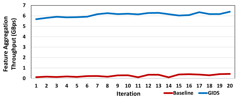
Figure 9. Feature aggregation throughput comparison between GIDS dataloader and the baseline dataloader for the first 20 iterations. One SSD is used for this measurement.

We conducted an extra evaluation to measure the impact of the storage latency on the feature aggregation performance of GIDS dataloader with the baseline dataloader when fetching feature data from a storage that consists of a single SSD for the IGB-Full dataset. For this evaluation, we measured the feature aggregation time for the first 20 iterations when both the GPU software-defined cache in GIDS dataloader and the CPU cache for the baseline were empty at iteration 1. Figure 9 shows that the feature aggregation bandwidth for GIDS dataloader was 5.6 GBps for iteration 1, while the baseline had a bandwidth of 0.05 GBps. As the peak SSD bandwidth for a 4KB cache-line is around 5.8 GBps, GIDS dataloader’s feature aggregation throughput shows that it can fully hide the storage latency. However, the baseline dataloader fails to hide the latency and faces significant overhead when the CPU cache is empty.

As the iterations progress, the feature aggregation bandwidth for both dataloaders increases as both the GPU cache for GIDS and the CPU cache for the baseline fill up with new data. GIDS dataloader reaches the saturation point after around iteration 10 since the GPU software-cache size is only 10GB. However, the CPU page cache capacity is 512GB and the page cache is still being warmed up after the first 20 iterations, so the feature aggregation process is not yet at the peak throughput at iteration 20 for the baseline. We also observed that when the page cache hit ratio is around 100%, the baseline dataloader can achieve around 5 GBps, which is still lower than the feature aggregation bandwidth of GIDS dataloader at iteration 1. This is because the CPU is over-utilized, and there are CPU software bottlenecks causing additional overhead (Min et al., 2021). Thus, GIDS dataloader outperforms the baseline dataloader even when the baseline dataloader is accessing a pre-loaded page cache.

4.3. Impact of the Window Buffering Cache Optimization

In this section, we present an evaluation of the impact of GPU software-defined cache optimization on the feature aggregation process. To conduct this evaluation, we compared the performance of GIDS with a basic GPU software-defined cache against GIDS with window buffering optimization. To ensure a fair comparison, we used the IGB-full dataset with the same Neighbor Sampling parameters and mini-batch size, and the size of the GPU cache was fixed at 10 GB for all configurations.

To accurately measure the impact of the window buffering technique, we varied the depth of the window buffer from 0 to 4, and then to 8 while evaluating the feature aggregation time and the GPU software-defined cache hit ratio. When the window buffer depth is 0, the GPU software-defined cache follows the random eviction policy, which serves as the baseline. Figure 10 displays the results, which show that the window buffering technique can improve the cache hit ratio. A window size of 4 improves the cache hit ratio by only 1.2$\times$ and the feature aggregation time by 1.04$\times$.

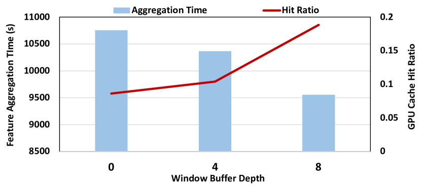
Figure 10. Performance comparison of feature aggregation process on GIDS dataloader for different window buffering depths.

Setting the window buffer depth too low, compared to the size of the GPU cache, can lead to a similar performance as random eviction. For instance, if the mini-batch size is 2 GB, and the GPU cache size is 10 GB, most of the node features from the previous four mini-batches still reside in the cache with a random eviction policy. Therefore, the optimal hit ratio with a window size of four is similar to random eviction, making it hard to achieve a meaningful performance gain.

When we increase the window buffer size to 8, the cache hit ratio improves by 2.19$\times$ over not having any window buffering, and the aggregation time decreases by 1.13$\times$. This is because the depth of the window buffer provides enough information about the cached node features that will be reused in future mini-batches to avoid evicting reusable cache-lines across mini-batches, which results in a substantial difference compared to random eviction. When the window buffer size is set to 8, the cached node features that the GPU cache can utilize are more than the node feature data that can fit into the GPU cache. Any further increase in the window buffer depth should be accompanied by an increased GPU cache.

Next, we compare the performance difference between window buffering and static cache-line pinning. For static cache-line pinning, GIDS dataloader pins 40% of the GPU cache with the feature data of the nodes with higher out-degree, as these nodes are more likely to be sampled and should be prioritized for pinning (Min et al., 2022; Lin et al., 2020).

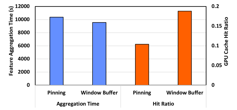
Figure 11. Feature aggregation performance comparison between window buffering and static cache-line pinning

As shown in Figure 11, the window buffering technique can outperform the cache-line pinning technique by 1.08x. Unlike static cache-line pinning, there is no overhead from graph preprocessing to mark specific segments as highly reusable whereas window buffering dynamically pins the cache-line based on the list of the sampled nodes. Moreover, the effectiveness of static cache-line pinning is highly influenced by the graph properties, whereas window buffering is significantly more flexible. As window buffering can provide higher performance and flexibility, GIDS leverages it for the default eviction policy.

However, there is a trade-off to consider when increasing the window buffer depth. First, there needs to be enough memory space for the window buffer. As the number of node samples for each mini-batch is around 1M, the size of the list of sampled nodes for a mini-batch is several megabytes. Although this is not a significantly large amount, larger window sizes increase the GPU memory requirement as the list of sampled nodes in the window buffer must be kept in the GPU memory for subsequent iterations. Additionally, a larger window size means a larger portion of the GPU cache will be pinned for future reuse, increasing the contention on the available cache-lines in the GPU software cache. Therefore, it is essential to carefully choose the window buffer size to ensure that the benefit of a higher cache hit ratio outweighs the overhead of a larger window buffer size. By default, the GIDS dataloader sets the depth of the window buffer to 8 based on the system environment. However, the window buffer depth is a tunable parameter that users can adjust based on the hardware environment, such as GPU memory size.

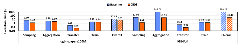
Figure 12. GNN training time breakdown of the DGL dataloader and GIDS dataloader with window buffering on the homogeneous graphs. One SSD is used in these measurements.

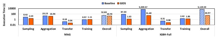
Figure 13. GNN training time breakdown of the DGL dataloader and GIDS dataloader with window buffering on the heterogeneous graphs. One SSD is used in these measurements.

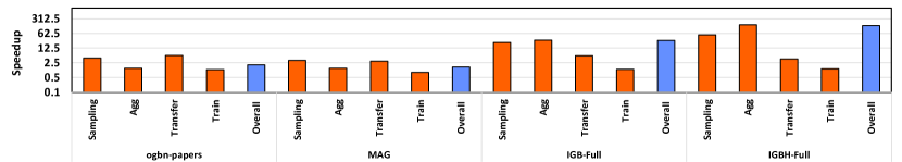
Figure 14. Speedup for each GNN training stage for GIDS dataloader with window buffering compared to the baseline dataloader.

4.4. Overall Performance

Figure 12 shows the execution time of each stage of GNN training time for the baseline and GIDS dataloader on homogeneous graphs, whereas their execution time on heterogeneous graphs is shown in Figure 13. Figure 14 shows the GIDS speedup compared to the baseline. For these measurements, one SSDs is used for GIDS. We will scale the number of SSDs in Section  4.5. As shown in Figure 14, our GIDS dataloader achieves a 29.98$\times$ and 1.38$\times$ speedup for the feature aggregation process compared to the DGL baseline dataloader on IGB-Full and ogbn-papers100M datasets. On heterogeneous graphs, our GIDS dataloader achieves a 160$\times$ and 1.37$\times$ speedup on IGBH-Full and MAG240M datasets, respectively.

These performance gains for the feature aggregation are attributed to the utilization of full storage bandwidth and leveraging GPU software-defined cache. The performance gain for IGB-Full and IGBH-Full datasets is substantially larger than that for ogbn-papers100M and MAG240M because the sizes of the latter two graphs are smaller than the CPU memory capacity, and thus the baseline does not incur significant number of page faults while training with these datasets. As a result, the performance gain for ogbn-papers100M and MAG240M mainly comes from the GPU software-defined cache. It is worth noting that the feature aggregation is bounded by the peak SSD bandwidth for this evaluation as a single SSD is used for both dataloaders. Section 4.5 and Section 4.7 show the overall GNN performance improvement and the time breakdown when GIDS leverages multiple SSDs to increase the storage bandwidth.

Our GIDS dataloader achieves a 22.98$\times$ and 3.25$\times$ speedup for the graph sampling process for IGB-Full and ogbn-papers100M. For heterogeneous graphs, our GIDS dataloader achieves a 53.55$\times$ and 6.3$\times$ speedup for the graph sampling process for IGBH-Full and MAG240M, respectively. This is because all graph structure data is pinned in the CPU memory so that the GPU can execute the graph sampling process via on-demand zero-copy data transfer. The transfer time is also reduced as the resulting mini-batch is kept in the GPU memory, so there is no need to transfer the feature data for the mini-batch from CPU to GPU with our GIDS dataloader. Finally, our GIDS dataloader does not modify any GNN training models so the training time remains constant between our approach and the baseline, aside from the variance caused by the random nature of the sampling process.

4.5. Storage Bandwidth Scalability

As the data preparation process is shifted from CPU to GPU on GIDS dataloader, the data preparation throughput can be accelerated by increasing the bandwidth to transfer data from storage to GPU. However, the peak SSD bandwidth often falls behind the PCIe bandwidth, limiting the maximum achievable throughput. To overcome this limitation, GIDS utilizes one of the features of the BaM system (Qureshi et al., 2023). This feature enables multiple SSDs to be connected to a single GPU and uniformly distributes I/O requests across all connected SSDs through round-robin scheduling. This amplifies the storage bandwidth and enables it to fully saturate the GPU’s PCIe x16 bandwidth. For instance, if four Intel Optane SSDs are connected to a single GPU, the collective SSD bandwidth would reach ~24 GBps, which nearly saturates the PCIe bandwidth.

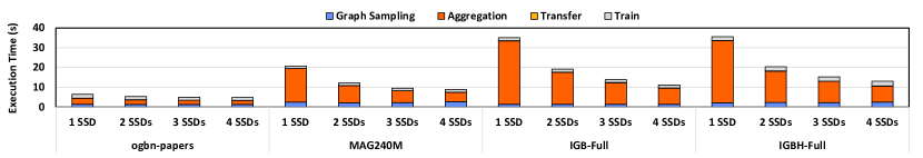
Figure 15. GNN training time breakdown of the DGL dataloader and GIDS dataloader with different numbers of SSDs.

Figure 15 shows the end-to-end (E2E) GNN training time with the time breakdown for GIDS dataloader as we scale the numbers of SSDs. With more SSDs, the collective SSD bandwidth increases, resulting in higher feature aggregation throughput. These results demonstrate that the feature aggregation process is limited by the storage bandwidth when the number of connected SSDs is less than four, and by the PCIe bandwidth when four SSDs are connected. When the PCIe bandwidth is fully saturated, the throughput is theoretically maximized when the data is not stored in the GPU memory. Since the baseline dataloader cannot even achieve the peak throughput of one SSD, its throughput does not improve with the additional SSDs. Furthermore, the pressure on the storage bandwidth for smaller graphs is relatively low, as the GPU software cache utilization is higher. Therefore, the performance gain from leveraging multiple SSDs is higher for larger graphs and the performance advantage of the GIDS dataloader is magnified by about 4$\times$ when using four SSDs for large graphs, as shown in Figure 15.

4.6. Comparison with UVA-based Approach

This section presents a performance comparison between the GIDS dataloader and the DGL dataloader, using the Unified Virtual Addressing (UVA) to enable GPU graph sampling and feature aggregation by pinning the graph data into the CPU memory. The IGB-Large dataset was used for evaluation since the UVA-based approach is limited to datasets smaller than the CPU memory capacity. The execution time of the UVA-based approach represents the lower bound of the GIDS approach without the software-defined cache as it does not incur any storage access latency and uses ample CPU memory bandwidth and can fully saturate the PCIe bandwidth by exploiting GPU memory-level parallelism during feature aggregation.

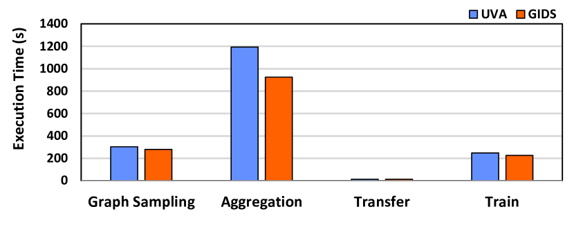
Figure 16. The comparison between UVA-based dataloader and GIDS dataloader with 4 SSDs for IGB-Large dataset

Figure 16 illustrates the normalized execution time of each GNN training stage for the two dataloaders. As shown in the figure, the feature aggregation time for GIDS dataloader is 0.72$\times$ compared to the baseline, a speedup of 1.29$\times$. Both dataloaders can fully saturate the PCIe bandwidth, but GIDS’s performance gain comes from its GPU software-defined cache and window buffering. The effectiveness of the GPU cache becomes more critical to the end-to-end (E2E) performance as the system is bounded by the PCIe bandwidth. Therefore, with GIDS and enough SSDs, there is no incentive for frameworks to try to keep the node features in the CPU memory even if they can fit. This is an important insight as this significantly reduces the cost for large-scale deployment of GNN in the industry.

4.7. GIDS Dataloader GNN Training Time-breakdown

Figure 17. GNN training time breakdown for GIDS dataloader. Four SSDs are used in this measurement.

In this section, we present the GNN training time breakdown for GIDS dataloader. To conduct this evaluation, we utilized four SSDs to saturate the PCIe-bandwidth, and employed the window buffering technique for the GPU software-defined cache. As shown in Figure 17, the disparity between the overheads of the GNN training pipeline stages is much less with GIDS than the baseline dataloader (Figure 3). For medium-scale graph datasets, namely ogbn-papers100M and MAG240M, with the GIDS dataloader the training time accounts for 32.5% and 16.9% of the total execution time, respectively, while it accounts for only 9.8% and 2% of the execution time when using the baseline dataloader. For large-scale graph datasets, IGB-Full and IGBH-Full, the training time takes 11.7% and 16.1%, respectively, when using GIDS dataloader, whereas the baseline dataloader with a 512GB CPU memory capacity takes only 0.18% and 0.04%. The results demonstrate that our proposed GIDS dataloader accelerates the data preparation process and much more closely matches the GPU training throughput.

5. Related Work

Several GNN specific applications and optimization have been proposed in the literature (Zeng et al., 2021; Miao et al., 2022; Hou et al., 2022; Vretinaris et al., 2021; Zhang et al., 2021b; Qiu et al., 2021). ROC (Jia et al., 2020), NeuGraph (Ma et al., 2019), and DSP (Cai et al., 2023) propose multi-GPU training system for large-scale GNN training. However, they require significant additional hardware resources and are not scalable solutions.

FeatGraph (Hu et al., 2020) and ZIPPER (Zhang et al., 2021a) propose tiling to mitigate the memory footprint during GNN training. FeatGraph reduces memory usage by utilizing graph partitioning and feature dimension tiling. Meanwhile, ZIPPER employs graph-native intermediate representation to optimize GNN, such as sparse graph tiling and redundant operation elimination. However, these approaches suffer from random accesses from GNN, leading to poor performance. Moreover, these solutions do not leverage GPU for the data preparation process.

AliGraph (Zhu et al., 2019), PaGraph (Lin et al., 2020), and Ginex (Park et al., 2022) use in-memory caching to reduce data transfer overhead. AliGraph and PaGraph cache high out-degree vertices in GPU memory to minimize data transfer between CPU and GPU. Ginex uses Belady’s algorithm with super-batch samples and pipelining techniques to hide the latency from specialized caching policies. However, these approaches rely on the CPU for the data preparation process and cannot fully hide storage latency.

Data Tiering (Min et al., 2022) uses weighted reverse PageRank to estimate the frequency of accesses during node sampling, improving GPU memory utilization. However, it requires all graph data to be stored in either CPU or GPU for GNN training execution, so not applicable for large-scale GNN training.

6. Conclusion

Training Graph Neural Networks (GNNs) on large-scale graph datasets is a challenging task due to their size exceeding the CPU memory capacity. Although distributed training is a possible solution, it is not cost-effective or even practical for many users. In this paper, we propose the GIDS dataloader, a GPU-oriented GNN training system that enables the training of large-scale graph datasets on a single machine. GIDS dataloader enables GPU threads to directly access storage and fully tolerates the long storage latency by exploiting the massive data level parallelism provided by GPUs. Moreover, GIDS dataloader further improves performance with a hybrid data placement strategy and by utilizing GPU memory as a software-defined cache with window buffering and cache-line pinning. By reducing the I/O overhead, GIDS dataloader can scale GNN training to datasets whose sizes are more than an order of magnitude larger than a single machine’s CPU memory capacity while achieving up to 392$\times$ speedups over the state-of-the-art dataloader for the overall execution of an end-to-end GNN training pipeline. Our measurements show that even after fully saturating the PCIe bandwidth and achieving a huge speedup over the baseline, the feature aggregation stage can still take significantly longer than the training stage for large-scale graphs, which indicates opportunities for further optimizations of the feature aggregation stage as potential future work.

References

- (1)
- HBM (2023) 2023. Nvidia ampere architecture in-depth. https://developer.nvidia.com/blog/nvidia-ampere-architecture-in-depth/
- Balin et al. (2023) Muhammed Fatih Balin, Kaan Sancak, and Umit V. Catalyurek. 2023. MG-GCN: A Scalable Multi-GPU GCN Training Framework. In Proceedings of the 51st International Conference on Parallel Processing (Bordeaux, France) (ICPP ’22). Association for Computing Machinery, New York, NY, USA, Article 79, 11 pages. https://doi.org/10.1145/3545008.3545082
- Bruna et al. (2014) Joan Bruna, Wojciech Zaremba, Arthur Szlam, and Yann LeCun. 2014. Spectral Networks and Locally Connected Networks on Graphs. arXiv:1312.6203 [cs.LG]
- Cai et al. (2023) Zhenkun Cai, Qihui Zhou, Xiao Yan, Da Zheng, Xiang Song, Chenguang Zheng, James Cheng, and George Karypis. 2023. DSP: Efficient GNN Training with Multiple GPUs. In Proceedings of the 28th ACM SIGPLAN Annual Symposium on Principles and Practice of Parallel Programming (Montreal, QC, Canada) (PPoPP ’23). 392–404.
- Defferrard et al. (2016) Michaël Defferrard, Xavier Bresson, and Pierre Vandergheynst. 2016. Convolutional Neural Networks on Graphs with Fast Localized Spectral Filtering (NIPS’16). Curran Associates Inc., Red Hook, NY, USA, 3844–3852.
- Fan et al. (2019) Wenqi Fan, Yao Ma, Qing Li, Yuan He, Eric Zhao, Jiliang Tang, and Dawei Yin. 2019. Graph Neural Networks for Social Recommendation. In The World Wide Web Conference (San Francisco, CA, USA) (WWW ’19). Association for Computing Machinery, New York, NY, USA, 417–426. https://doi.org/10.1145/3308558.3313488
- Fey and Lenssen (2019) Matthias Fey and Jan Eric Lenssen. 2019. Fast Graph Representation Learning with PyTorch Geometric. arXiv:1903.02428 [cs.LG]
- Garcia and Bruna (2018) Victor Garcia and Joan Bruna. 2018. Few-Shot Learning with Graph Neural Networks. arXiv:1711.04043 [stat.ML]
- Grattarola and Alippi (2021) Daniele Grattarola and Cesare Alippi. 2021. Graph Neural Networks in TensorFlow and Keras with Spektral [Application Notes]. Comp. Intell. Mag. 16, 1 (feb 2021), 99–106. https://doi.org/10.1109/MCI.2020.3039072
- Hamilton et al. (2017) William L. Hamilton, Rex Ying, and Jure Leskovec. 2017. Inductive Representation Learning on Large Graphs. In Proceedings of the 31st International Conference on Neural Information Processing Systems (Long Beach, California, USA) (NIPS’17). Curran Associates Inc., Red Hook, NY, USA, 1025–1035.
- Hou et al. (2022) Pei-Yu Hou, Daniel R. Korn, Cleber C. Melo-Filho, David R. Wright, Alexander Tropsha, and Rada Chirkova. 2022. Compact Walks: Taming Knowledge-Graph Embeddings with Domain- and Task-Specific Pathways. In Proceedings of the 2022 International Conference on Management of Data (Philadelphia, PA, USA) (SIGMOD ’22). Association for Computing Machinery, New York, NY, USA, 458–469. https://doi.org/10.1145/3514221.3517903
- Hu et al. (2021) Weihua Hu, Matthias Fey, Marinka Zitnik, Yuxiao Dong, Hongyu Ren, Bowen Liu, Michele Catasta, and Jure Leskovec. 2021. Open Graph Benchmark: Datasets for Machine Learning on Graphs. arXiv:2005.00687 [cs.LG]
- Hu et al. (2020) Yuwei Hu, Zihao Ye, Minjie Wang, Jiali Yu, Da Zheng, Mu Li, Zheng Zhang, Zhiru Zhang, and Yida Wang. 2020. FeatGraph: A Flexible and Efficient Backend for Graph Neural Network Systems. In Proceedings of the International Conference for High Performance Computing, Networking, Storage and Analysis (Atlanta, Georgia) (SC ’20). IEEE Press, Article 71, 13 pages.
- Jia et al. (2020) Zhihao Jia, Sina Lin, Mingyu Gao, Matei Zaharia, and Alex Aiken. 2020. Improving the accuracy, scalability, and performance of graph neural networks with roc. Proceedings of Machine Learning and Systems 2 (2020), 187–198.
- Keskar et al. (2017) Nitish Shirish Keskar, Dheevatsa Mudigere, Jorge Nocedal, Mikhail Smelyanskiy, and Ping Tak Peter Tang. 2017. On Large-Batch Training for Deep Learning: Generalization Gap and Sharp Minima. arXiv:1609.04836 [cs.LG]
- Khatua et al. (2023) Arpandeep Khatua, Vikram Sharma Mailthody, Bhagyashree Taleka, Tengfei Ma, Xiang Song, and Wen mei Hwu. 2023. IGB: Addressing The Gaps In Labeling, Features, Heterogeneity, and Size of Public Graph Datasets for Deep Learning Research. arXiv:2302.13522 [cs.LG]
- Kipf and Welling (2017) Thomas N. Kipf and Max Welling. 2017. Semi-Supervised Classification with Graph Convolutional Networks. In Proceedings of the 5th International Conference on Learning Representations (Palais des Congrès Neptune, Toulon, France) (ICLR ’17).
- Lin et al. (2020) Zhiqi Lin, Cheng Li, Youshan Miao, Yunxin Liu, and Yinlong Xu. 2020. PaGraph: Scaling GNN Training on Large Graphs via Computation-Aware Caching. In Proceedings of the 11th ACM Symposium on Cloud Computing (Virtual Event, USA) (SoCC ’20). Association for Computing Machinery, New York, NY, USA, 401–415. https://doi.org/10.1145/3419111.3421281
- Liu et al. (2020) Zhiwei Liu, Yingtong Dou, Philip S. Yu, Yutong Deng, and Hao Peng. 2020. Alleviating the Inconsistency Problem of Applying Graph Neural Network to Fraud Detection. In Proceedings of the 43rd International ACM SIGIR Conference on Research and Development in Information Retrieval (Virtual Event, China) (SIGIR ’20). Association for Computing Machinery, New York, NY, USA, 1569–1572. https://doi.org/10.1145/3397271.3401253
- Ma et al. (2019) Lingxiao Ma, Zhi Yang, Youshan Miao, Jilong Xue, Ming Wu, Lidong Zhou, and Yafei Dai. 2019. Neugraph: Parallel Deep Neural Network Computation on Large Graphs. In Proceedings of the 2019 USENIX Conference on Usenix Annual Technical Conference (Renton, WA, USA) (USENIX ATC ’19). USENIX Association, USA, 443–457.
- Miao et al. (2022) Xupeng Miao, Yining Shi, Hailin Zhang, Xin Zhang, Xiaonan Nie, Zhi Yang, and Bin Cui. 2022. HET-GMP: A Graph-Based System Approach to Scaling Large Embedding Model Training. In Proceedings of the 2022 International Conference on Management of Data (Philadelphia, PA, USA) (SIGMOD ’22). Association for Computing Machinery, New York, NY, USA, 470–480. https://doi.org/10.1145/3514221.3517902
- Min et al. (2022) Seung Won Min, Kun Wu, Mert Hidayetoglu, Jinjun Xiong, Xiang Song, and Wen-mei Hwu. 2022. Graph Neural Network Training and Data Tiering. In Proceedings of the 28th ACM SIGKDD Conference on Knowledge Discovery and Data Mining (Washington DC, USA) (KDD ’22). Association for Computing Machinery, New York, NY, USA, 3555–3565. https://doi.org/10.1145/3534678.3539038
- Min et al. (2021) Seung Won Min, Kun Wu, Sitao Huang, Mert Hidayetoğlu, Jinjun Xiong, Eiman Ebrahimi, Deming Chen, and Wen mei Hwu. 2021. PyTorch-Direct: Enabling GPU Centric Data Access for Very Large Graph Neural Network Training with Irregular Accesses. arXiv:2101.07956 [cs.LG]
- Pal et al. (2020) Aditya Pal, Chantat Eksombatchai, Yitong Zhou, Bo Zhao, Charles Rosenberg, and Jure Leskovec. 2020. PinnerSage: Multi-Modal User Embedding Framework for Recommendations at Pinterest. In Proceedings of the 26th ACM SIGKDD International Conference on Knowledge Discovery and Data Mining (Virtual Event, CA, USA) (KDD ’20). Association for Computing Machinery, New York, NY, USA, 2311–2320. https://doi.org/10.1145/3394486.3403280
- Park et al. (2022) Yeonhong Park, Sunhong Min, and Jae W. Lee. 2022. Ginex: SSD-Enabled Billion-Scale Graph Neural Network Training on a Single Machine via Provably Optimal in-Memory Caching. Proc. VLDB Endow. 15, 11 (jul 2022), 2626–2639. https://doi.org/10.14778/3551793.3551819
- Preprint et al. (2021) A Preprint, Yunsheng Shi, Zhengjie Huang, and Weibin Li. 2021. R-UNIMP: SOLUTION FOR KDDCUP 2021 MAG240M-LSC.
- Qiu et al. (2021) Jiezhong Qiu, Laxman Dhulipala, Jie Tang, Richard Peng, and Chi Wang. 2021. LightNE: A Lightweight Graph Processing System for Network Embedding. In Proceedings of the 2021 International Conference on Management of Data (Virtual Event, China) (SIGMOD ’21). Association for Computing Machinery, New York, NY, USA, 2281–2289. https://doi.org/10.1145/3448016.3457329
- Qureshi et al. (2023) Zaid Qureshi, Vikram Sharma Mailthody, Isaac Gelado, Seungwon Min, Amna Masood, Jeongmin Park, Jinjun Xiong, C. J. Newburn, Dmitri Vainbrand, I-Hsin Chung, Michael Garland, William Dally, and Wen-mei Hwu. 2023. GPU-Initiated On-Demand High-Throughput Storage Access in the BaM System Architecture. In Proceedings of the 28th ACM International Conference on Architectural Support for Programming Languages and Operating Systems, Volume 2 (Vancouver, BC, Canada) (ASPLOS 2023). Association for Computing Machinery, New York, NY, USA, 325–339. https://doi.org/10.1145/3575693.3575748
- Rajbhandari et al. (2021) Samyam Rajbhandari, Olatunji Ruwase, Jeff Rasley, Shaden Smith, and Yuxiong He. 2021. ZeRO-Infinity: Breaking the GPU Memory Wall for Extreme Scale Deep Learning. In Proceedings of the International Conference for High Performance Computing, Networking, Storage and Analysis (St. Louis, Missouri) (SC ’21). Association for Computing Machinery, New York, NY, USA, Article 59, 14 pages. https://doi.org/10.1145/3458817.3476205
- Ramezani et al. (2020) Morteza Ramezani, Weilin Cong, Mehrdad Mahdavi, Anand Sivasubramaniam, and Mahmut T. Kandemir. 2020. GCN Meets GPU: Decoupling "When to Sample" from "How to Sample". In Proceedings of the 34th International Conference on Neural Information Processing Systems (Vancouver, BC, Canada) (NIPS’20). Curran Associates Inc., Red Hook, NY, USA, Article 1552, 11 pages.
- Rossi et al. (2022) Andrea Rossi, Donatella Firmani, Paolo Merialdo, and Tommaso Teofili. 2022. Explaining Link Prediction Systems Based on Knowledge Graph Embeddings. In Proceedings of the 2022 International Conference on Management of Data (Philadelphia, PA, USA) (SIGMOD ’22). Association for Computing Machinery, New York, NY, USA, 2062–2075. https://doi.org/10.1145/3514221.3517887
- Veličković et al. (2018) Petar Veličković, Guillem Cucurull, Arantxa Casanova, Adriana Romero, Pietro Liò, and Yoshua Bengio. 2018. Graph Attention Networks. arXiv:1710.10903 [stat.ML]
- Vretinaris et al. (2021) Alina Vretinaris, Chuan Lei, Vasilis Efthymiou, Xiao Qin, and Fatma Özcan. 2021. Medical Entity Disambiguation Using Graph Neural Networks. In Proceedings of the 2021 International Conference on Management of Data (Virtual Event, China) (SIGMOD ’21). Association for Computing Machinery, New York, NY, USA, 2310–2318. https://doi.org/10.1145/3448016.3457328
- Wang et al. (2023) Chunyang Wang, Desen Sun, and Yuebin Bai. 2023. PiPAD. In Proceedings of the 28th ACM SIGPLAN Annual Symposium on Principles and Practice of Parallel Programming. ACM. https://doi.org/10.1145/3572848.3577487
- Wang et al. (2019) Jianyu Wang, Rui Wen, Chunming Wu, Yu Huang, and Jian Xiong. 2019. FdGars: Fraudster Detection via Graph Convolutional Networks in Online App Review System. In Companion Proceedings of The 2019 World Wide Web Conference (San Francisco, USA) (WWW ’19). Association for Computing Machinery, New York, NY, USA, 310–316. https://doi.org/10.1145/3308560.3316586
- Wang et al. (2020) Kuansan Wang, Zhihong Shen, Chiyuan Huang, Chieh-Han Wu, Yuxiao Dong, and Anshul Kanakia. 2020. Microsoft Academic Graph: When experts are not enough. Quantitative Science Studies 1, 1 (02 2020), 396–413. https://doi.org/10.1162/qss_a_00021 arXiv:https://direct.mit.edu/qss/article-pdf/1/1/396/1760880/qss_a_00021.pdf
- Wang et al. (2022) Qiange Wang, Yanfeng Zhang, Hao Wang, Chaoyi Chen, Xiaodong Zhang, and Ge Yu. 2022. NeutronStar: Distributed GNN Training with Hybrid Dependency Management. In Proceedings of the 2022 International Conference on Management of Data (Philadelphia, PA, USA) (SIGMOD ’22). Association for Computing Machinery, New York, NY, USA, 1301–1315. https://doi.org/10.1145/3514221.3526134
- Wilson and Martinez (2003) D. Randall Wilson and Tony R. Martinez. 2003. The General Inefficiency of Batch Training for Gradient Descent Learning. Neural Netw. 16, 10 (dec 2003), 1429–1451. https://doi.org/10.1016/S0893-6080(03)00138-2
- Wu et al. (2023) Qitian Wu, Yiting Chen, Chenxiao Yang, and Junchi Yan. 2023. Energy-based Out-of-Distribution Detection for Graph Neural Networks. arXiv:2302.02914 [cs.LG]
- Ye et al. (2021) Chang Ye, Yuchen Li, Bingsheng He, Zhao Li, and Jianling Sun. 2021. GPU-Accelerated Graph Label Propagation for Real-Time Fraud Detection. In Proceedings of the 2021 International Conference on Management of Data (Virtual Event, China) (SIGMOD ’21). Association for Computing Machinery, New York, NY, USA, 2348–2356. https://doi.org/10.1145/3448016.3452774
- Zeng et al. (2021) Hanqing Zeng, Hongkuan Zhou, Ajitesh Srivastava, Rajgopal Kannan, and Viktor Prasanna. 2021. Accurate, efficient and scalable training of Graph Neural Networks. J. Parallel and Distrib. Comput. 147 (jan 2021), 166–183. https://doi.org/10.1016/j.jpdc.2020.08.011
- Zhang et al. (2020) Dalong Zhang, Xin Huang, Ziqi Liu, Jun Zhou, Zhiyang Hu, Xianzheng Song, Zhibang Ge, Lin Wang, Zhiqiang Zhang, and Yuan Qi. 2020. AGL: A Scalable System for Industrial-Purpose Graph Machine Learning. Proc. VLDB Endow. 13, 12 (aug 2020), 3125–3137. https://doi.org/10.14778/3415478.3415539
- Zhang and Chen (2018) Muhan Zhang and Yixin Chen. 2018. Link Prediction Based on Graph Neural Networks. In Proceedings of the 32nd International Conference on Neural Information Processing Systems (Montréal, Canada) (NIPS’18). Curran Associates Inc., Red Hook, NY, USA, 5171–5181.
- Zhang et al. (2021b) Wentao Zhang, Yu Shen, Yang Li, Lei Chen, Zhi Yang, and Bin Cui. 2021b. ALG: Fast and Accurate Active Learning Framework for Graph Convolutional Networks. In Proceedings of the 2021 International Conference on Management of Data (Virtual Event, China) (SIGMOD ’21). Association for Computing Machinery, New York, NY, USA, 2366–2374. https://doi.org/10.1145/3448016.3457325
- Zhang et al. (2021a) Zhihui Zhang, Jingwen Leng, Shuwen Lu, Youshan Miao, Yijia Diao, Minyi Guo, Chao Li, and Yuhao Zhu. 2021a. ZIPPER: Exploiting Tile- and Operator-level Parallelism for General and Scalable Graph Neural Network Acceleration. arXiv:2107.08709 [cs.AR]
- Zhao et al. (2015) Jishen Zhao, Sheng Li, Jichuan Chang, John L. Byrne, Laura L. Ramirez, Kevin Lim, Yuan Xie, and Paolo Faraboschi. 2015. Buri: Scaling Big-Memory Computing with Hardware-Based Memory Expansion. ACM Trans. Archit. Code Optim. 12, 3, Article 31 (oct 2015), 24 pages. https://doi.org/10.1145/2808233
- Zheng et al. (2021) Da Zheng, Chao Ma, Minjie Wang, Jinjing Zhou, Qidong Su, Xiang Song, Quan Gan, Zheng Zhang, and George Karypis. 2021. DistDGL: Distributed Graph Neural Network Training for Billion-Scale Graphs. arXiv:2010.05337.
- Zhu et al. (2019) Rong Zhu, Kun Zhao, Hongxia Yang, Wei Lin, Chang Zhou, Baole Ai, Yong Li, and Jingren Zhou. 2019. AliGraph: A Comprehensive Graph Neural Network Platform. Proc. VLDB Endow. 12, 12 (aug 2019), 2094–2105. https://doi.org/10.14778/3352063.3352127