Upper bounds on the maximum admissible level of noise in zeroth-order optimisation

Abstract

In this paper, we leverage an information-theoretic upper bound on the maximum admissible level of noise (MALN) in convex Lipschitz-continuous zeroth-order optimisation to establish corresponding upper bounds for classes of strongly convex and smooth problems. We derive these bounds through non-constructive proofs via optimal reductions. Furthermore, we demonstrate that by employing a one-dimensional grid-search algorithm, one can devise an algorithm for simplex-constrained optimisation that offers a superior upper bound on the MALN compared to the case of ball-constrained optimisation and estimates asymptotic in dimensionality.

1 Introduction

The problem of interest in this paper is $\min_{x\in S}f(x)$, such that $S\subset\mathbb{R}^{n}$ is a compact and convex set and $f:\mathbb{R}^{n}\to\mathbb{R}$ is a convex continuous function. Note that these conditions imply the existence of $x^{*}\in S$ satisfying $f(x^{*})=\inf_{x\in S}f(x)$. We assume that the only oracle for function $f$ is a zeroth-order oracle that provides evaluations with additive noise. Specifically, it provides $f(x)+\xi$ for a given $x\in S$, where $|\xi|\leqslant\delta$ [1, 2]. Function $f$ can be treated as approximately convex [3], implying the existence of a convex function $g$ such that $|f(x)-g(x)|\leqslant\delta$ holds for all $x\in S$. Problems of this nature arise when the gradient of $f$ cannot be efficiently computed, either explicitly or automatically. This situation occurs, for instance, when $x$ serves as a hyperparameter for a model, or when $f(x)$ represents the outcome of a real-life experiment with the variable $x$ under control [4, 5, 6].

The assessment of the complexity of these problems should encompass upper bounds on noise $\delta$ [3, 7], in addition to lower bounds on the number of oracle calls or iterations. While the latter informs us about the time consumption required to solve the worst-case problem using the best algorithm, the former informs us whether we can attain the desired level of accuracy. For an intuitive example, solving a problem with arbitrary precision becomes implausible if the computation of $f$ is subject to machine precision or other instrumental errors.

This introduces a new trade-off that was absent in first-order optimisation: a trade-off between the time resources allocated for the algorithm and those allocated for the computation of $f$. Alternatively, a trade-off emerges between the overall time and memory resources, particularly when the primary source of noise stems from rounding errors in floating-point arithmetic.

An information-theoretic upper bound on the MALN has been established for functions $f$ that satisfy the Lipschitz continuity condition [3]. However, obtaining upper bounds for other classes of optimization problems, such as those that are strongly convex or have Lipschitz-continuous gradients, from this Lipschitz continuity result is not straightforward, as is often the case with information-theoretic proofs.

On the other hand, it is noteworthy that optimal iteration complexities across different problem classes are interconnected through ``reductions'', which are algorithmic extensions that efficiently transform optimal algorithms for one class into optimal algorithms for another [8]. In our study, we leverage these optimal reductions to derive bounds on level of noise. Moreover, we substantiate that these bounds indeed serve as tight upper bounds, employing a non-constructive argument and providing the algorithms that admit this level of noise.

Upper bounds on noise are independent of lower bounds on the number of iterations. In other words, an algorithm that demonstrates an optimal convergence rate may, in general, necessitate less admissible noise compared to a less efficient algorithm. This disparity is particularly evident in the case of the grid-search algorithm, which selects the most suitable approximation of the minimum from closely spaced probes. This algorithm's MALN is proportional to the desired accuracy. However, as the size of the grid grows exponentially, the algorithm's complexity becomes non-polynomial in terms of both the dimensionality $n$ and the accuracy parameter $\varepsilon^{-1}$.

There is the lower bound on the MALN proportional to the desired accuracy divided by a coefficient which is polynomial on $n$ [9], Section 9.4.2. To enhance this lower bound, we attempt to refine it for a more focused class of functions constrained within a simplex. This is achieved by reducing these problems to multi-level one-dimensional problems and leveraging edge effects to diminish the grid size. Consequently, this approach yields a lower bound on noise that is proportional to the desired accuracy divided by the dimensionality.

2 Methods

In the course of our study we address the following research questions:

• Can upper bounds on the MALN for the class of functions $A$ be derived from those of the class of functions $B$ using optimal reductions?

• What are the upper bounds on the MALN for the class of functions with: a) small-dimensional domain spaces; b) aspheric domain sets?

Optimal reductions of optimisation algorithms were introduced in [8]. In Section 3, we comprehensively address RQ₁ for the classes of convex ($A$) and strongly-convex ($B$). We also partially solve this question for the classes of non-smooth ($A$) and smooth ($B$) problems. This analysis yields upper bounds on noise applicable to strongly-convex and smooth problems, respectively.

The discrepancy between the theoretical asymptotic upper bound on the MALN and the actual noise that optimisation algorithms can handle in low-dimensional problems is elucidated in Section 5. We present an example of a non-optimal algorithm for optimisation over a segment, which exhibits lower sensitivity to noise than anticipated from theory. While this doesn't fully resolve RQ_2a, it does highlight that the actual upper bound for problems with small dimensions is higher than previously considered.

Furthermore, we delve into the connection between this phenomenon and optimisation over feasible sets that deviate from the conventional spherical shape, particularly in the context of the $n$-dimensional simplex. This discussion addresses RQ_2b specifically for simplex feasible sets.

Assumption 1.

The assumptions which define corresponding classes of optimisation problems under consideration, are provided below.

1. Convexity. For given convex set $S\subset\mathbb{R}^{n}$ it holds that

   $$\langle\nabla f(x),y-x\rangle\leqslant f(y)-f(x),\quad\forall x,y\in S.$$ (C)

2. Lipschitz continuity. For given set $S\subset\mathbb{R}^{n}$ there exists $M>0$, such that

   $$f(y)-f(x)\leqslant M\|y-x\|_{2},\quad\forall x,y\in S.$$ (LC)

3. Smoothness. For given set $S\subset\mathbb{R}^{n}$ there exists $L>0$, such that

   $$\langle\nabla f(y)-\nabla f(x),y-x\rangle\leqslant L\|y-x\|_{2}^{2},\quad\forall x,y\in S.$$ (LS)

4. Strong-growth. For given set $S\subset\mathbb{R}^{n}$ and extremum $x^{*}\in S$ there exists $\nu\in[1,+\infty]$, $\mu>0$ and convex function $g:S\to\mathbb{R}$, such that

   $$g(x)=f(x)-\frac{\mu}{2}\|x-x^{*}\|_{2}^{\nu},\quad\forall x\in S.$$ (SG)

It is important to note that the strong-growth condition employed in this paper is more stringent than the standard strong-growth condition, expressed as $\frac{\mu}{2}\|x-x^{*}\|_{2}^{\nu}\leqslant f(x)-f(x^{*})$ for all $x\in S$. Consequently, the upper bound derived in the corresponding theorem applies to this refined sub-class. It is worth noting that this upper bound remains applicable to broader class as well. In fact, by expanding the class of admissible functions, the maximal allowable noise only decreases. In Section 4, we elucidate the gap between the derived upper bounds and MALN of particular state-of-the-art algorithms. In the strongly-growing non-smooth case, this gap disappears.

3 Upper bounds on the MALN obtained by the optimal reductions

Definition 1 (Classes of convex functions).

For convex set $S\subset\mathbb{R}^{n}$, $M>0$, $L>0$, $\mu\geqslant 0$ and $\nu\in[1,+\infty]$, the following classes are defined

1. Class $\mathcal{F}_{Lip}^{M}(S)\subset C^{1}(S)\cap Cvx(S)$ of $M$-Lipschitz continuous functions, which satisfy Assumptions C and LC;

2. Class $\mathcal{F}_{Lip}^{M,\mu,\nu}(S)\subset\mathcal{F}_{Lip}^{M}(S)$ of $M$-Lipschitz continuous $\mu$-strongly-growing functions, which satisfy Assumptions C, LC and SG;

3. Class $\mathcal{F}_{Smooth}^{L}(S)\subset C^{2}(S)\cap Cvx(S)$ of functions with $L$-Lipschitz continuous gradient, which satisfy Assumptions C and LS;

4. Class $\mathcal{F}_{Smooth}^{L,\mu,\nu}(S)\subset\mathcal{F}_{Smooth}^{L}(S)$ of $(\mu,\nu)$-strongly-growing functions with $L$-Lipschitz continuous gradient, which satisfy Assumptions C, LS and SG,

where $Cvx(S)$ is a set of convex functions, which satisfy Assumption C.

In [3], the authors obtained an upper bound on the MALN solely for the first of the classes, precisely, for Lipschitz continuous convex functions, through the explicit construction of a worst-case function. However, extending this approach to derive upper bounds on the MALN for other classes remains nontrivial, and such worst-case functions for each class of functions have yet to be determined. The result of this paper resolves this question by deriving all upper bounds from one in a non-constructive manner. The fruits of this approach are summarised in the Table 1.

Tab. 1: Known and derived in this paper upper bounds on the MALN for different classes of convex functions.

$\delta=O(\dots)$	convex	$(\mu,\nu)$-strongly-growing
$M$-Lipschitz	$\displaystyle\max\left\{\frac{\varepsilon^{2}}{\sqrt{n}MR},\frac{\varepsilon}{n}\right\}$, [3]	$\displaystyle\max\left\{\frac{\mu^{1/\nu}\varepsilon^{2-1/\nu}}{\sqrt{n}M},\frac{\varepsilon}{n}\right\}$, Thm 1
$L$-smooth	$\displaystyle\max\left\{\frac{\varepsilon^{3/2}}{\sqrt[4]{n}\sqrt{L}R},\frac{\varepsilon}{n}\right\}$, Thm 2	$\displaystyle\max\left\{\frac{\mu^{1/\nu}\varepsilon^{3/2-1/\nu}}{\sqrt[4]{n}\sqrt{L}},\frac{\varepsilon}{n}\right\}$, Thm 3

3.1 Noise contraction while reducing the strongly-growing case to the convex one

Following the reasoning of restarts technique [8], we need to ensure

$$P\left(\left\|x^{N_{k}}-x^{*}\right\|_{2}\geqslant 2^{-1/\nu}\left\|x^{N_{k-1}}-x^{*}\right\|_{2}\right)\leqslant\alpha,$$ (1)

where $N_{k}$ is the number of iterations made by algorithm after the restart $k$, and $0<\alpha<1$. There are two cases, corresponding to different dominating term in formula of $\delta_{k}$:

1. If $\varepsilon_{k}\geqslant M\left\|x^{N_{k-1}}-x^{*}\right\|_{2}/\sqrt{n}$, it holds that

   $$\frac{\mu}{2}\left\|x^{N_{k}}-x^{*}\right\|_{2}^{\nu}\stackrel{{\scriptstyle\eqref{eq:growth}}}{{\leqslant}}f(x^{N_{k}})-f(x^{*})\leqslant\frac{M\left\|x^{N_{k-1}}-x^{*}\right\|_{2}}{\sqrt{N_{k}}}+n^{1/4}\sqrt{M\delta_{k}\left\|x^{N_{k-1}}-x^{*}\right\|_{2}},$$

   where the second inequality is implied by the optimal convergence rate in the Lipschitz continuous case and known upper bound on the MALN for it, and holds with probability greater than $1/2$. implies the following choice of parameters:

   $$\delta_{k}=\frac{\gamma^{2}\varepsilon_{k}^{2}}{\sqrt{n}M\left\|x^{N_{k-1}}-x^{*}\right\|_{2}},\quad N_{k}=\frac{M^{2}\left\|x^{N_{k-1}}-x^{*}\right\|_{2}^{2}}{(1-\gamma)^{2}\varepsilon_{k}^{2}},\quad\varepsilon_{k}=\frac{\mu}{4}\left\|x^{N_{k-1}}-x^{*}\right\|^{\nu}_{2},$$

   which results in such a dependence of noise on the distance from extremum

   $$\delta_{k}=\frac{\gamma^{2}\mu^{2}\left\|x^{N_{k-1}}-x^{*}\right\|_{2}^{2\nu-1}}{16\sqrt{n}M}=2^{-k(2-1/\nu)}\cdot\frac{\gamma^{2}\mu^{2}R^{2\nu-1}}{16\sqrt{n}M}.$$ (2)

   Corresponding condition on $\varepsilon_{k}$ is reduced to $\|x^{N_{k-1}}-x^{*}\|_{2}^{\nu-1}\geqslant 4M/\left(\mu\sqrt{n}\right)$, or $\|x^{N_{k-1}}-x^{*}\|$ is arbitrary and $n\geqslant 16M^{2}/\mu^{2}$, if $\nu=1$.

2. If $\varepsilon_{k}\leqslant M\left\|x^{N_{k-1}}-x^{*}\right\|_{2}/\sqrt{n}$, in other words, when operation of the algorithm in the regime described above ensures $\|x^{N_{k-1}}-x^{*}\|^{\nu-1}\leqslant 4M/\left(\mu\sqrt{n}\right)$, or if $\nu=1$, for all $n\leqslant 16M^{2}/\mu^{2}$, it holds that

   $$\frac{\mu}{2}\left\|x^{N_{k}}-x^{*}\right\|_{2}^{\nu}\stackrel{{\scriptstyle\eqref{eq:growth}}}{{\leqslant}}f(x^{N_{k}})-f(x^{*})\leqslant\frac{M\left\|x^{N_{k-1}}-x^{*}\right\|_{2}}{\sqrt{N_{k}}}+n\delta_{k}$$

   with probability greater than $1/2$, which implies the following choice of parameters, for some $0<\gamma<1$:

   $$\delta_{k}=\frac{\gamma\varepsilon_{k}}{n},\quad N_{k}=\frac{M^{2}\left\|x^{N_{k-1}}-x^{*}\right\|_{2}^{2}}{(1-\gamma)^{2}\varepsilon_{k}^{2}},\quad\varepsilon_{k}=\frac{\mu}{4}\left\|x^{N_{k-1}}-x^{*}\right\|^{\nu}_{2},$$

   which results in such a dependence of noise on the distance from extremum

   $$\delta_{k}=\frac{\gamma\mu\left\|x^{N_{k-1}}-x^{*}\right\|^{\nu}_{2}}{4n}\leqslant 2^{-k}\cdot\frac{\gamma\mu R^{\nu}}{4n}.$$ (3)

In order to satisfy the probabilistic condition (1), each restart shall be re-performed $\log_{2}1/\alpha$ times from the same initial point, which guarantees that at least one of the obtained results will satisfy the bound on a function value discrepancy.

Since the former condition is ensured by the proper choice of parameters, we have

$$f(x^{N_{k}})-f(x^{*})\leqslant\frac{\mu}{4}\left\|x^{N_{k-1}}-x^{*}\right\|^{\nu}_{2}\leqslant 2^{-k-1}\mu R^{\nu}\leqslant\varepsilon$$

with probability $1-\alpha k$, where

$$k=\log_{2}{\frac{\mu R^{\nu}}{\varepsilon}}-1.$$ (4)

By plugging this estimation of number of iterations into (3) and (2), and setting $\alpha=\beta/k$, for each $n\in\mathbb{N}$, $M>0$, $\mu>0$, $\nu\in[1,+\infty]$, ball $S\subset\mathbb{R}^{n}$ containing extremum $x^{*}$, we obtain

Theorem 1 (Upper bound on the MALN for $M$-Lipschitz $(\mu,\nu)$-strongly-growing problems).

For any algorithm, given $\varepsilon>0$, and

$$\delta>\max\left\{\frac{\mu^{1/\nu}\varepsilon^{2-1/\nu}}{\sqrt{n}M},\frac{\varepsilon}{n}\right\},$$

there exists a function $f\in\mathcal{F}_{Lip}^{M,\mu,\nu}(S)$ such that the algorithm will not obtain $x$ such that $f(x)-f(x^{*})\leqslant\varepsilon$ in $poly\left(n,\varepsilon^{-1}\right)$ iterations with probability greater than $\beta$, for any $0<\beta<1$.

• All the bounds obtained using the optimal reductions should be proven by contradiction. We assume that there exist an algorithm, $\varepsilon>0$, and corresponding $\delta$, such that for every $f\in\mathcal{F}_{Lip}^{M,\mu,\nu}(S)$ the algorithm obtains $x$ such that $f(x)-f(x^{*})\leqslant\varepsilon$ in $poly\left(n,\varepsilon^{-1}\right)$ iterations with probability greater than $1-\beta$.

  Then, we should lead this statement to the contradiction. We will show that some function $g\in\mathcal{F}_{Lip}^{M}(S)$ together with algorithm given in aforementioned negative assumption contradict an upper bound on the MALN from [3]. Specifically, given algorithm will obtain $x$ such that $g(x)-g(x^{*})\leqslant\varepsilon$ in $poly\left(n,\varepsilon^{-1}\right)$ iterations even if $\delta$ is greater than the upper bound on the MALN. For arbitrary $f$, let us define $g$ by the following equation: $g(x)=f(x)-\frac{\mu}{2}\|x-x^{*}\|_{2}^{\nu}$, where $\mu=\frac{\varepsilon}{R^{\nu}}$. $g$ has the following properties: $g\in\mathcal{F}_{Lip}^{M}(S)$, and $x^{*}$ is an extremum of $g$.

  Now, let us prove that $g$ contradicts [3]. Given the algorithm applicable to any function $f\in\mathcal{F}_{Lip}^{M,\mu,\nu}(S)$ for given $\mu>0$ from negative assumption, we obtain algorithm applicable to function $g$, by applying optimal reduction, called regularisation, from class of $M$-Lipschitz convex to class of $M$-Lipschitz $(\frac{\varepsilon}{2R^{\nu}},\nu)$-strongly-growing functions. Specifically, the algorithm obtains, with probability greater than $1-\beta$, such $x$ that $f(x)-f(x^{*})\leqslant\varepsilon/2$ in $poly\left(n,\varepsilon^{-1}\right)$ iterations for $f\in\mathcal{F}_{Lip}^{M,\mu,\nu}(S)$ (it holds due to the (SG)) defined by $f(x)=g(x)+\frac{\mu}{2}\cdot\|x-x^{*}\|_{2}^{\nu}$, where $\mu=\frac{\varepsilon}{R^{\nu}}$. The obtained inexact solution $x$ is such that $g(x)-g(x^{*})\leqslant\varepsilon$ with probability greater than $1-\beta$ [8]. Note that if zeroth-order oracle $O_{g}:(x,\xi)\mapsto g(x)+\xi$ is provided as part of the problem statement for function $g$, there exists an oracle $O_{f}:(x,\xi)\mapsto O_{g}(x,\xi)+\frac{\mu}{2}\cdot\|x-x^{*}\|_{2}^{\nu}$, despite the lack of possibility to construct it explicitly due to the absence of $x^{*}$. Oracle $O_{f}$ allows the correct stating the optimisation problem for function $f$, which is necessary for applying optimal reduction. On the other hand, by negative assumption, $\delta$ is greater than the MALN for the class $\mathcal{F}_{Lip}^{M,\mu,\nu}(S)$. Finally, substituting $\mu$ into the formula for $\delta$ and re-solving regularised problem $1/\left(\log_{2}1/\beta\right)$ times from the same initial point if $\beta>1/2$, we find that

  $$\delta>\max\left\{\frac{\varepsilon^{2}}{\sqrt{n}MR},\frac{\varepsilon}{n}\right\},$$

  which contradicts the theoretical upper bound on the MALN from [3]. ∎

3.2 Issues of reducing the smooth case to the non-smooth one

For each $n\in\mathbb{N}$, $L>0$, ball $S\subset\mathbb{R}^{n}$ containing extremum $x^{*}$, it holds the

Theorem 2 (Upper bound on the MALN for $L$-smooth convex problems).

For any algorithm, given $\varepsilon>0$, and

$$\delta>\max\left\{\frac{\varepsilon^{3/2}}{\sqrt[4]{n}\sqrt{L}R},\frac{\varepsilon}{n}\right\},$$

there exists $f\in\mathcal{F}_{Smooth}^{L}(S)$ such that algorithm will not obtain $x$ such that $f(x)-f(x^{*})\leqslant\varepsilon$ in $poly\left(n,\varepsilon^{-1}\right)$ iterations with probability greater than $\beta$, for any $0<\beta<1$.

• Assume that there exist algorithm, $\varepsilon>0$, and corresponding $\delta$, such that for every $f\in\mathcal{F}_{Smooth}^{L}(S)$ algorithm obtains $x$ such that $f(x)-f(x^{*})\leqslant\varepsilon$ in $poly\left(n,\varepsilon^{-1}\right)$ iterations with probability greater than $1-\beta$.

  This proof differs from that of Theorem 1 in that it takes a particular function $g$ and its smooth counterpart $f$ to lead the assumption to contradiction. This particular function is the worst-case function $g=\tilde{f}_{w}$ of the class $\mathcal{F}_{Lip}^{M}(S)$ which is defined in [3], Construction 4.2. Note that $M=1$ for this construction, but it is scalable to an arbitrary $M>0$, so it is enough to consider only $M=1$ here.

  Let us introduce function $f$ defined by $f(x)=\mathbb{E}_{e}[f(x+\gamma e)]$, where $e\propto\mathcal{U}(S^{n})$ is uniformly random vector drawn from unit ball according to probability density function $p$, and $\gamma=\varepsilon/(2M)$. This transformation is known as $\ell_{2}$-ball smoothing [10]. It holds for all $x\in S$ that $|f(x)-g(x)|\leqslant\varepsilon/2$, and $f\in\mathcal{F}_{Smooth}^{L}(S)$ with $L=\frac{2\sqrt{n}M^{2}}{\varepsilon}$. According to the assumption made above, some algorithm can be applied to function $f$ to obtain $x$ such that $f(x)-f(x^{*})\leqslant\varepsilon/2$ in $poly\left(n,\varepsilon^{-1}\right)$ iterations with probability greater than $1-\beta$. The obtained $x$ is such that $g(x)-g(x^{*})\leqslant\varepsilon$ with probability greater than $1-\beta$. On the other hand, $\delta$ is greater than the MALN for the class $\mathcal{F}_{Smooth}^{L}(S)$. Substituting $L$ into the formula for $\delta$ and re-solving smoothed problem $1/\left(\log_{2}1/\beta\right)$ times from the same initial point if $\beta>1/2$, we find that

  $$\delta>\max\left\{\frac{\varepsilon^{2}}{\sqrt{n}MR},\frac{\varepsilon}{n}\right\},$$

  which contradicts the theoretical upper bound on the MALN from [3].

  The remaining part of the proof is providing on the base of the oracle $O_{g}:(x,\xi)\mapsto g(x)+\xi$ corresponding to the function $g$ some oracle $O_{f}:S\times\mathbb{R}\mapsto\mathbb{R}$ for the function $f$, such that it holds for any $|\xi|\leq\delta$ that $|O_{f}(x,\xi)-f(x)|=O(\delta)$ and computational complexity per call of $O_{f}$ does not exceed $poly\left(n,\epsilon^{-1}\right)$ (if it does not, overall computational complexity of the algorithm applicable to the function $g$ is bounded by the composition of two functions from $poly\left(n,\epsilon^{-1}\right)$, which is in $poly\left(n,\epsilon^{-1}\right)$ in turn). $\mathbb{E}_{e}[\cdot]$ is an integral over the set $S^{n}$, so it can be approximated using celebrated Monte–Carlo method. Its efficiency depends on the following ingredients:

  1. the fine-grained enough partition $S^{n}\subseteq S_{1}\sqcup\dots\sqcup S_{N}\subset\mathbb{R}^{n}$ such that it holds for some constants $c_{1},c_{2}>0$ that $\int_{S_{i}}dp\leqslant c_{1}/N$ and $\sup_{x,y\in S_{i}}\|x-y\|_{2}\leqslant c_{2}/N^{1/n}$, for every $i=1,...,N$;

  2. the appropriate number $N$ of samples which guarantees that absolute discrepancy between obtained approximation $\theta(x)$ and $f(x)$ never exceeds $\delta$.

  Fortunately, the partition is not to be recomputed on each iteration, so it does not contribute to the per call computational complexity, and one only needs to prove its existence. One can obtain, using Maurey's empirical method for covering with $\ell_{1}$-balls and then Artstein–Milman–Szarek theorem to move to $\ell_{\infty}$-balls, that, given the length of the edge $c_{3}$, the number $N$ of hyper-cubes with this edge required to cover $\ell_{2}$-ball is upper bounded by $\log N=O\left(n\log\frac{1}{c_{3}^{2}n}\right)$ [11]. By choosing $c_{3}=\Theta(1/\sqrt{n})$ we provide the first ingredient. Behind the second ingredient there is a transition from probabilistic guarantee of bounded variance, typical for Monte–Carlo methods, to an absolute bound on $|\theta(x)-f(x)|$. Using [12], Section 4.1.2 Theorem 3 and Chebyshev's inequality, one can obtain the bound on probability of big deviations:

  $$P(|\theta(x)-f(x)|>\sqrt{n^{2}(c_{1}c_{2})^{2}M^{2}+\mathbb{D}[\xi]}N^{-1/2}/\alpha)\leqslant\alpha^{2},$$

  for any $0<\alpha<1$. Assume that the number of iterations the algorithm applied to the function $f$ performs does not exceed $T\in poly\left(n,\varepsilon^{-1}\right)$. By choosing $\alpha=\sqrt{\beta/T}$, one ensures that

  $$P\left(|\theta(x_{t})-f(x_{t})|>\sqrt{n^{2}(c_{1}c_{2})^{2}M^{2}+\mathbb{D}[\xi]}N^{-1/2}\sqrt{T/\beta}\right)\leqslant\beta,$$

  for all $t=1,...,T$. To complete the second ingredient, one needs to choose $N$ according to the following formula:

  $$N=\left\lceil\frac{n^{2}TM^{2}(c_{1}c_{2})^{2}}{\beta\delta^{2}}+\frac{1}{\beta}\right\rceil+1=O\left(poly\left(n,\varepsilon^{-1}\right)\right),$$

  where the Popoviciu's inequality $\mathbb{D}[\xi]\leqslant\delta^{2}$ is used, and that $1/\delta$ is upper bounded with $poly\left(n,\varepsilon^{-1}\right)$, by the assumption, was taken into account. $N$ is the number of $O_{g}$ calls in one call of $O_{f}:(x,\xi)\mapsto\theta(x)$. ∎

Remark 1.

One flaw of the Theorem 1-like proof. The proof sketch presented in the earlier preprint https://arxiv.org/abs/2306.16371v2 of this paper shared the same scheme of proof as that in Theorem 1, but was working for only those functions $f$ which gradient is $L$-Lipschitz continuous on the whole $\mathbb{R}^{n}$. If the gradient of function $f$ ceases to be $L$-Lipschitz continuous outside the prescribed set $S$, conjugate function $f^{*}$ is not strongly convex, and one cannot construct its unsmoothed counterpart, function $g$, like it was done in Theorem 1. This would be possible if there existed an extension of function $f$ to the whole $\mathbb{R}^{n}$ which preserves the $L$-Lipschitz continuity of gradient of the function $f$. Such an extension has neither been constructed nor shown to be non-existent yet.

Direct reduction to the strongly-convex case. One more possibility to proof this upper bound is applying regularisation from class of $M$-Lipschitz convex to class of $M$-Lipschitz $\frac{\varepsilon}{2R^{2}}$-strongly-convex functions. This optimal reduction might apply the algorithm to regularised Legendre–Fenchel conjugate of the function $g$ to find an extremum of Legendre–Fenchel conjugate $g^{*}$ of the convex function $g$. This approach works if only primal-dual algorithms are considered. Specifically, if algorithm for function $f$ is at the same time the algorithm for $f^{*}$ due to generating both sequences of primal and dual variables.

3.3 Combination of the smooth and the strongly-growing generalisations

The following theorem shares the scheme of proof of Theorem 1, which was described with all intuitive remarks, so does not require repetition.

1. If $\varepsilon_{k}\geqslant L\|x^{N_{k-1}}-x^{*}\|_{2}^{2}/n^{3/2}$, or for any $\|x^{N_{k-1}}-x^{*}\|_{2}$ if $\nu=2$ and $n\geqslant 4^{2/3}\left(L/\mu\right)^{2/3}$, it holds that

   $$\frac{\mu}{2}\|x^{N_{k}}-x^{*}\|_{2}^{\nu}\stackrel{{\scriptstyle\eqref{eq:growth}}}{{\leqslant}}f(x^{N_{k}})-f(x^{*})\leqslant\frac{L\|x^{N_{k-1}}-x^{*}\|_{2}^{2}}{N_{k}^{2}}+\sqrt[3]{\sqrt{n}L\delta_{k}^{2}\|x^{N_{k-1}}-x^{*}\|_{2}^{2}}$$

   with probability greater than $1-\alpha$, where $0<\alpha<1$, which implies the following choice of parameters:

   $$\delta_{k}=\sqrt{\frac{\alpha^{3}\varepsilon_{k}^{3}}{\sqrt{n}L\|x^{N_{k-1}}-x^{*}\|_{2}^{2}}},\quad N_{k}=\sqrt{\frac{L\|x^{N_{k-1}}-x^{*}\|^{2}}{(1-\alpha)\varepsilon_{k}}},\quad\varepsilon_{k}=\frac{\mu}{4}\|x^{N_{k-1}}-x^{*}\|_{2}^{\nu},$$

   which results in such a dependence of noise on distance from extremum

   $$\delta_{k}=\sqrt{\frac{\alpha^{3}\mu^{3}}{\sqrt{n}L}}\frac{\|x^{N_{k-1}}-x^{*}\|_{2}^{3\nu/2-1}}{8}=2^{-k(3/2-1/\nu)}\cdot\sqrt{\frac{\alpha^{3}\mu^{3}}{\sqrt{n}L}}\frac{R^{3\nu/2-1}}{8}.$$ (5)

2. If $\varepsilon_{k}\leqslant L\|x^{N_{k-1}}-x^{*}\|_{2}^{2}/n^{3/2}$, or for any $\|x^{N_{k-1}}-x^{*}\|_{2}$ if $\nu=2$ and $n\leqslant 4^{2/3}\left(L/\mu\right)^{2/3}$, it holds that

   $$\frac{\mu}{2}\|x^{N_{k}}-x^{*}\|_{2}^{\nu}\leqslant f(x^{N_{k}})-f(x^{*})\leqslant\frac{L\|x^{N_{k-1}}-x^{*}\|_{2}^{2}}{N_{k}^{2}}+n\delta_{k}$$

   with probability greater than $1-\alpha$, which implies the following choice of parameters:

   $$\delta_{k}=\frac{\alpha\varepsilon_{k}}{n},\quad N_{k}=\sqrt{\frac{L\|x^{N_{k-1}}-x^{*}\|_{2}^{2}}{(1-\alpha)\varepsilon_{k}}},\quad\varepsilon_{k}=\frac{\mu}{4}\|x^{N_{k-1}}-x^{*}\|_{2}^{\nu},$$

   which results in such a dependence of noise on distance from extremum

   $$\delta_{k} =\frac{\alpha\mu\|x^{N_{k-1}}-x^{*}\|_{2}^{\nu}}{4n}\leqslant 2^{-k}\cdot\frac{\alpha\mu R^{\nu}}{4n}.$$ (6)

Note, that if $\nu<2$, the second regime operates before the first one, for bigger $\|x^{N_{k-1}}-x^{*}\|$, while if $\nu<2$, the order is opposite.

By plugging (4) into (6) and (5), and setting $\alpha=\beta/k$, for each $n\in\mathbb{N}$, $L>0$, $\mu>0$, $\nu\in[1,+\infty]$, ball $S\subset\mathbb{R}^{n}$ containing extremum $x^{*}$, we obtain

Theorem 3 (Upper bound on the MALN for $L$-smooth $(\mu,\nu)$-strongly-growing problems).

For any algorithm, given $\varepsilon>0$, and

$$\delta>\max\left\{\frac{\mu^{1/\nu}\varepsilon^{3/2-1/\nu}}{\sqrt[4]{n}\sqrt{L}},\frac{\varepsilon}{n}\right\},$$

there exists $f\in\mathcal{F}_{Smooth-Lip}^{L,M,\mu,\nu}(S)$ such that algorithm will not obtain $x$ such that $f(x)-f(x^{*})\leqslant\varepsilon$ in $poly\left(n,\varepsilon^{-1}\right)$ iterations with probability greater than $\beta$, for any $0<\beta<1$.

• Assume that there exist algorithm, $\varepsilon>0$, and corresponding $\delta$, such that for every $f\in\mathcal{F}_{Smooth-Lip}^{L,M,\mu,\nu}(S)$ algorithm obtains $x$ such that $f(x)-f(x^{*})\leqslant\varepsilon$ in $poly\left(n,\varepsilon^{-1}\right)$ iterations with probability greater than $1-\beta$.

  For arbitrary $f$, let us define $g$ by the following equation: $g(x)=f(x)-\frac{\mu}{2}\|x-x^{*}\|_{2}^{\nu}$, where $\mu=\frac{\varepsilon}{R^{\nu}}$. $g$ has the following properties: $g\in\mathcal{F}_{Lip}^{M}(S)$, and $x^{*}$ is an extremum of $g$. We apply regularisation from class of $M$-Lipschitz convex functions with $L$-Lipschitz gradient to class of $M$-Lipschitz $(\frac{\varepsilon}{2R^{\nu}},\nu)$-strongly-growing functions with $L$-Lipschitz gradient, to obtain an algorithm applicable to $g$. The algorithm obtains, with probability greater than $1-\beta$, such $x$ that $f(x)-f(x^{*})\leqslant\varepsilon/2$ in $poly\left(n,\varepsilon^{-1}\right)$ iterations for $f\in\mathcal{F}_{Smooth}^{L,\mu,\nu}(S)$ defined by $f(x)=g(x)+\frac{\mu}{2}\cdot\|x-x^{*}\|_{2}^{\nu}$, where $\mu=\frac{\varepsilon}{R^{\nu}}$. The obtained inexact solution $x$ is such that $g(x)-g(x^{*})\leqslant\varepsilon$ with probability greater than $1-\beta$ [8]. Oracle $O_{f}:S\times\mathbb{R}\to\mathbb{R}$ for problem statement for function $f$, to which the former problem for function $g$ is reduced, is constructed from the given oracle $O_{g}:S\times\mathbb{R}\to\mathbb{R}$ for the former problem similarly to that in proof of Theorem 1. On the other hand, by substituting $\mu$ into the formula for $\delta$, we find that

  $$\delta>\max\left\{\frac{\varepsilon^{3/2}}{\sqrt[4]{n}\sqrt{L}R},\frac{\varepsilon}{n}\right\},$$

  which contradicts the upper bound on the MALN from the Theorem 2. ∎

4 The MALN of particular algorithms

In this section, we compare the upper bounds on the MALN for different classes of optimisation problems, obtained in Section 3, with the MALN estimates achieved by particular algorithms.

Convex case. In [13] authors propose an algorithm for solving problems of the class $\mathcal{F}_{Lip}^{M}(S)$ such that the MALN of this algorithm is $\frac{\varepsilon^{2}}{\sqrt{n}MR}$. This estimate corresponds to the upper bound on the MALN from [3]. If the function also belongs to the class $\mathcal{F}_{Smooth}^{L}(S)$, the algorithm proposed in [14], Subsection 3.2, which exploits the $\ell_{2}$-ball smoothing approach, improves an estimate of the MALN up to $\frac{\varepsilon^{3/2}}{\sqrt{nL}R}$. This MALN estimate does not match the upper bound on the MALN obtained in Theorem 2. However, one may share the hypothesis that this estimate of the MALN is optimal, while the upper bound suggested in Theorem 2 is not tight due to the technical obstacles in proofs not yet resolved.

Strongly-growing case. The MALN of the algorithm proposed in [15] is $\frac{\mu^{1/\nu}\varepsilon^{2-1/\nu}}{\sqrt{n}M}$. Using the same approach as described in [14], Subsection 3.2, one can achieve the MALN $\frac{\mu^{1/\nu}\varepsilon^{3/2-1/\nu}}{\sqrt{nL}}$ while applied to the functions from the class $\mathcal{F}_{Smooth}^{L,\mu,\nu}(S)$ by an appropriate modification of the algorithm proposed in [15]. This MALN, again, does not meet the upper bound on the MALN given by the Theorem 3.

It is noteworthy that these algorithms are optimal in terms of the number of iterations and the overall number of oracle calls. In [15, 14, 13] authors address the stochastic problem formulation, which indicates that the upper bounds are robust not only in the deterministic setting, but also in the stochastic setting. Furthermore, the robustness of these upper bounds extends to stochastic problems featuring heavy-tailed distributions, as detailed in [14].

5 Low-dimensional case and the role of a grid-search

5.1 One-dimensional grid-search

Definition 2 (Classes of non-convex 1-dimensional and separable Lipschitz problems).

For compact interval $I\subsetneq\mathbb{R}$, convex set $S\subset\mathbb{R}^{n}$, and $M>0$, the following classes are defined

1. Class $\mathcal{F}_{NC-Lip}^{M}(S)\subset C^{1}(S)$ of $M$-Lipschitz continuous functions, which satisfy Assumption LC;

2. Class $\mathcal{F}_{1-Lip}^{M}(I)\subset\mathcal{F}_{NC-Lip}^{M}(I)$ of 1-dimensional $M$-Lipschitz continuous functions, which satisfy Assumption LC;

3. Class $\mathcal{F}_{Sep-Lip}^{M}(S)\subset\mathcal{F}_{NC-Lip}^{M}(S)$ of functions $f$ defined by $f(x)=\sum_{i=1}^{n}f_{i}(x_{i})$, where $f_{i}\in\mathcal{F}_{1-Lip}^{M}(I_{i})$ are $M$-Lipschitz continuous functions, which satisfy Assumption LC.

Note that $\mathcal{F}_{1-Lip}^{M}(I)\subset\mathcal{F}_{Sep-Lip}^{M}(S)$, if there exist $x_{1},...,x_{i-1},x_{i+1},...,x_{n}$ such that $\{x_{1}\}\times\dotsi\times\{x_{i-1}\}\times I\times\{x_{i+1}\}\times\dotsi\times\{x_{n}\}\subset S$.

Theorem 4 (Lower bound on the MALN for separable $M$-Lipschitz problems).

There exists algorithm, such that for every $\varepsilon>0$, given

$$\delta\leqslant\frac{\varepsilon}{2n},$$

and function $f\in\mathcal{F}_{Sep-Lip}^{M}(S)$, algorithm will obtain $x$ such that $f(x)-f(x^{*})\leqslant\varepsilon$ in $\frac{n^{2}RM}{\varepsilon}\in poly\left(n,\varepsilon^{-1}\right)$ iterations.

• Note that its enough to proof the statement in the case of $n=1$. Indeed, statements of the theorem for $n>1$ follows if we solve 1-dimensional problem with respect to $x_{1}$ with accuracy $\varepsilon/(2n)$ on $\text{proj}_{1}S$, then with respect to $x_{2}$ on $\text{proj}_{2}\{x\in S:x_{1}=x_{1}^{*}\}$, et cetera.

  

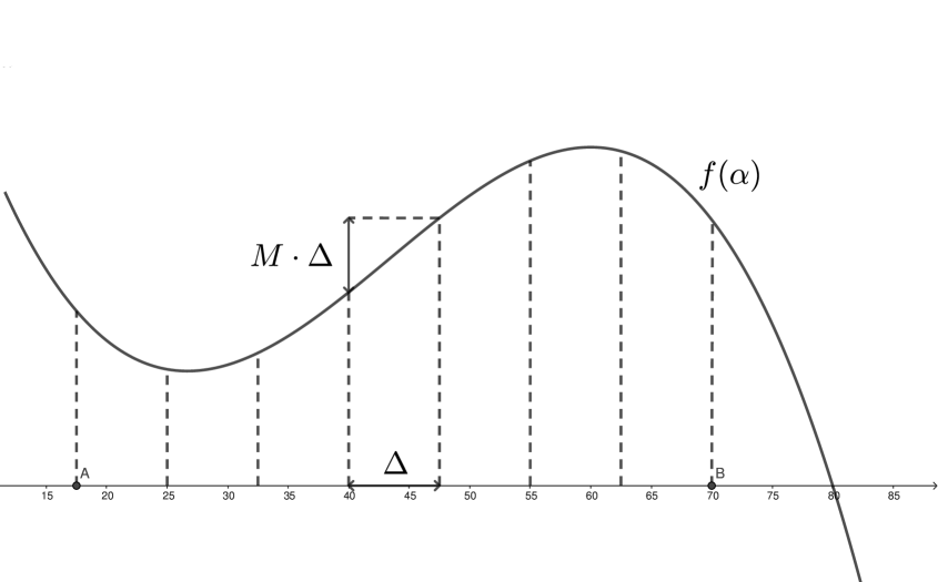
  Fig. 1: Example of one-dimensional $M$-Lipschitz continuous function with overlaid grid

  

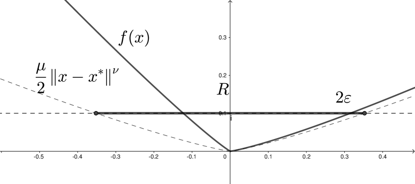
  Fig. 2: Bound for feasible set of consequent 1-dimensional problems

  So, let's proof the result for $f\in\mathcal{F}_{1-Lip}^{M}(I)$. There exists such an algorithm: take $\Delta=\varepsilon/(2M)$ and overlay a $\Delta$-grid on $I=[a,b]$, i.e. $I_{\Delta}=\left\{a,...,a+i\cdot\Delta,...,a+\lfloor\frac{b-a}{\Delta}\rfloor\cdot\Delta,b\right\}$. Illustration is provided on Figure 1. Then choose $x=\arg\min_{x\in I_{\Delta}}f(x)$ (this takes $\leqslant\lceil\frac{b-a}{\Delta}\rceil+1$ function evaluations). Due to Assumption LC it holds that $f(x)-f(x^{*})\leqslant M\cdot\Delta+\delta\leqslant\varepsilon$. ∎

5.2 Connection to the optimisation on Euclidean simplex

Definition 3 (Euclidean simplex).

Euclidean n-simplex $\sigma[p_{1},...,p_{n+1}]\subset\mathbb{R}^{n+1}$ spanned by points $p_{1},...,p_{n+1}\in\mathbb{R}^{n+1}$ is $\left\{x\in\mathbb{R}^{n+1}:\exists\alpha_{1},...,\alpha_{n+1}>0,\sum_{i=1}^{n+1}\alpha_{i}=1,x=\sum_{i=1}^{n+1}\alpha_{i}p_{i}\right\}$.

Note that $\sigma[p_{1},...,p_{n+1}]$ is contained in some hyperplane. To specify a point on an Euclidean simplex it is required to specify $n-1$ coordinates. Set of coefficients $\alpha_{1},...,\alpha_{n}$ defines a point $x$ in $\sigma[p_{1},...,p_{n+1}]$ and is called barycentric coordinates of $x$.

Theorem 5 (Lower bound on the MALN for $M$-Lipschitz $(M,1)$-strongly-growing problems on Euclidean simplex).

There exists algorithm, such that for every $\varepsilon>0$, given

$$\delta\leqslant\frac{\varepsilon}{n+1},$$

points $p_{1},...,p_{n}\in\mathbb{R}^{n+1}$ such that $\|p_{i}\|=1,i=1,...,n$, and function $f\in\mathcal{F}_{Lip}^{M,M,1}(\sigma[p_{1},...,p_{n},0])$, algorithm will obtain $x$ such that $f(x)-f(x^{*})\leqslant\varepsilon$ in $poly\left(n,\varepsilon^{-1}\right)$ iterations.

• Original optimisation problem for function $f$ can be equivalently rewritten as optimisation problem for function $g$ in barycentric coordinates:

  $$x(\alpha_{1},...,\alpha_{n})=\sum_{i=1}^{n}\alpha_{i}p_{i}+\left(1-\sum_{i=1}^{n}\alpha_{i}\right)p_{n+1},$$

  $$\min_{\alpha_{n}\in[0,1]}\dotsi\min_{\alpha_{2}\in[0,1-\alpha_{n}]}\min_{\alpha_{1}\in\left[0,1-\sum_{i=2}^{n}\alpha_{i}\right]}\left\{g(\alpha_{1},...,\alpha_{n})=f(x(\alpha_{1},...,\alpha_{n}))\right\}.$$ (7)

  If $f$ is $M$-Lipschitz continuous, $g$ is coordinate-wise $\left(M\|p_{i}-p_{n+1}\|\right)$-Lipschitz continuous: indeed,

  $$|g(\alpha_{1},...,\alpha_{i}+\alpha,...,\alpha_{n})-g(\alpha_{1},...,\alpha_{i},...,\alpha_{n})|$$

  $$=|f(x(\alpha_{1},...,\alpha_{n})+\alpha(p_{i}-p_{n+1}))-f(x(\alpha_{1},...,\alpha_{n}))|\leqslant M\|p_{i}-p_{n+1}\||\alpha|.$$

  Statement of the theorem follows if we solve 1-dimensional problem with respect to $\alpha_{1}$ with accuracy $\varepsilon/(n+1)$ and given $\delta$, use this solution in the oracle to solve 1-dimensional problem for function $\min_{\alpha_{1}}g(\alpha_{1},\alpha_{2},...,\alpha_{n})$ with respect to $\delta_{2}$ with accuracy $\varepsilon/(n+1)$ and noise $2\varepsilon/(n+1)$, …, and finally use solution of the $(n-1)$-th problem in the oracle to solve 1-dimensional problem for function $\min_{\alpha_{n-1}}\dotsi\min_{\alpha_{1}}g(\alpha_{1},...,\alpha_{n})$ with respect to $\delta_{n}$ with accuracy $\varepsilon/(n+1)$ and noise $n\varepsilon/(n+1)$. Similarly to Theorem 5, Lipschitz constants do not affect bound on noise / resulting accuracy, but only density of the grid.

  If the size of feasible set for each 1-dimensional problem is upper bounded by 1, number of function's evaluations will be in the worst case $\leqslant\left(\frac{(n+1)M}{\varepsilon}\right)^{n}\cdot\prod_{i=1}^{n}\|p_{i}-p_{n+1}\|$, which is not $poly\left(n,\varepsilon^{-1}\right)$. If we allow such an asymptotic for the number of iterations, provided bound for $\delta$ is lower bound for all bounded sets and all $f\in\mathcal{F}_{NC-Lip}^{M}(S)$.

  Without loss of generality we assume $\|p_{i}\|=1,i=1,...,n$ and $p_{n+1}=0$ hereinafter to simplify the form of the proofs. Note that algorithm makes $\frac{(n+1)M}{\varepsilon}$ probes to solve 1-level 1-dimensional problem. Each probe makes $\alpha_{n}$ bigger by $\frac{\varepsilon}{(n+1)M}$, and makes feasible set for 2-level smaller by $\frac{\varepsilon}{(n+1)M}$, correspondingly. If 2-level problem makes $T_{2}(R)$ function's evaluations on feasible set of size $R$, 1-level problem will require in total $\sum_{i=0}^{\lceil\frac{(n+1)M}{\varepsilon}\rceil}T_{2}(1-\frac{i\varepsilon}{(n+1)M})$. This can be iterated to result in

  $$\sum_{i_{1}=0}^{\lceil N\rceil}\sum_{i_{2}=0}^{\left\lceil N\left(1-\frac{i_{1}}{N}\right)\right\rceil}\dotsi\sum_{i_{n-1}=0}^{\left\lceil N\left(1-\frac{i_{1}+\dotsi+i_{n-2}}{N}\right)\right\rceil}T_{n}\left(1-\frac{i_{1}+\dotsi+i_{n-1}}{N}\right)\leqslant$$

  $$\qquad\leqslant\sum_{i_{1}=0}^{N+1}\sum_{i_{2}=0}^{N-i_{1}+1}\dotsi\sum_{i_{n-1}=0}^{N-(i_{1}+\dotsi+i_{n-2})+1}\sum_{i_{n}=0}^{N-(i_{1}+\dotsi+i_{n-1})+1}1=$$

  $$\qquad=\sum_{i_{1}=0}^{N+1}\sum_{i_{2}=i_{1}}^{N+1}\dotsi\sum_{i_{n}=i_{n-1}}^{N+1}1=\binom{N+n+1}{n}=O\left(\frac{1}{\sqrt{n}}\left(\frac{\mathrm{e}M}{\varepsilon}\right)^{n}\right)$$

  function's evaluations, where $N=\frac{(n+1)M}{\varepsilon}$. If we allow such an asymptotic for the number of iterations, provided bound for $\delta$ is lower bound for all bounded sets triangulable into $poly\left(n,\varepsilon^{-1}\right)$ simplices and all $f\in\mathcal{F}_{NC-Lip}^{M}(S)$.

  If we now exploit Assumption SG, we can avoid most of probes taken into account in the last formula. We can use the proximity of 1-dimensional subproblems being solved on the same level to localise next subproblem given the solution of previous one.

  In case of $n=2$ we need to solve one 1-dimensional subproblem corresponding to $\alpha+\frac{i\varepsilon}{(n+1)M}$ with accuracy $\varepsilon/(n+1)$ by the overlaying full $\left(\frac{\varepsilon}{(n+1)M}\right)$-grid to get $x_{i}=x(\alpha_{1},...,\alpha_{n})$ such that $f(x)-f(x_{i}^{*})\leqslant\varepsilon/(n+1)$, where $x_{i}^{*}$ is minimum point on a segment $I_{i}=\left\{x(\alpha_{1},\alpha_{2})\in\sigma[p_{1},p_{2},p_{3}]:\alpha_{1}=\alpha+\frac{i\varepsilon}{(n+1)M}\right\}$ and $R$ is length of feasible interval. Point $x^{\prime}_{i+1}$ on the segment $I_{i+1}=\left\{x(\alpha_{1},\alpha_{2})\in\sigma[p_{1},p_{2},p_{3}]:\alpha_{1}=\alpha+\frac{(i+1)\varepsilon}{(n+1)M}\right\}$ obtained by translation of $x_{i}$ parallel to line $\alpha_{2}=0$ will be centre of localised feasible set. Besides, for every pair of arbitrary point $x_{i}$ and $x^{\prime}_{i+1}$ obtained by procedure above, it holds that $\|x_{i}-x^{\prime}_{i+1}\|_{2}\leqslant\varepsilon/((n+1)M)$. By Assumption LC, $f(x^{\prime}_{i+1})\leqslant f(x_{i})+\varepsilon/(n+1)$. Besides, Assumptions LC implies that $f(x^{*}_{i+1})>f(x^{*}_{i})-\varepsilon/(n+1)$ (otherwise, one could parallel translate $x^{*}_{i+1}$ into the point $x$ on $I_{i}$ such that $f(x)<f(x^{*}_{i})$, which is not possible). Thus, $f(x^{\prime}_{i+1})-f(x^{*}_{i+1})\leqslant 2\varepsilon/(n+1)$. By Assumption SG we get that $\|x^{\prime}_{i+1}-x^{*}_{i+1}\|_{2}\leqslant 2^{1+1/\nu}\cdot\left(\frac{\varepsilon}{\mu(n+1)}\right)^{1/\nu}$, which means that one should take feasible interval of length $2^{2+1/\nu}\cdot\left(\frac{\varepsilon}{\mu(n+1)}\right)^{1/\nu}$ centred in $x^{\prime}_{i+1}$.

  Since the minimum $x_{i+1}$ found on such a feasible interval will coincide with if it would be found on full interval, postnext problem can be provided with the feasible interval of the same length but centred in $x^{\prime}_{i+2}$, et cetera. In total, this procedure requires at most

  $$\frac{(n+1)M}{\varepsilon}+\left(\frac{(n+1)M}{\varepsilon}-1\right)\cdot 2^{2+1/\nu}\cdot\left(\frac{\varepsilon}{\mu(n+1)}\right)^{1/\nu}\frac{(n+1)M}{\varepsilon}$$

  $$\qquad=O\left(\frac{(n+1)M}{\varepsilon}+\frac{(n+1)^{2-1/\nu}M^{2}}{\mu^{1/\nu}\varepsilon^{2-1/\nu}}\right)$$

  probes, which only for $\nu=1$ takes the form $O\left(\frac{M(n+1)}{\varepsilon}\left(1+\frac{M}{\mu}\right)\right)$ with unchanged degree of $\varepsilon$ and $n$.

  To get number of iterations required for $n>2$ such an algorithms will need

  $$O\left(\frac{(n+1)M}{\varepsilon}\left(1+\frac{3M}{\mu}\left(1+\frac{3M}{\mu}\left(1+\dotsi\right)\right)\right)\right)=O\left(\frac{(n+1)M}{\varepsilon}\left(\frac{3M}{\mu}\right)^{n}\right)$$

  probes. If we allow such an asymptotic for the number of iterations, provided bound for $\delta$ is lower bound for all bounded sets and all $f\in\mathcal{F}_{Lip}^{M,\mu,1}(S)$.

  Finally, we can exploit some edge effects inherent in the simplex. Firstly, we always can choose interval for the first subproblem which requires full grid overlaying to be small enough, so that $1+\frac{3M}{\mu}+\dotsi+\left(\frac{3M}{\mu}\right)^{n-1}$ turns into just $\left(\frac{3M}{\mu}\right)^{n-1}$. Secondly, some choices of $\alpha_{i}$ lead to subproblems that are not to be solved. Indeed, if current feasible interval length is $0<R\leqslant 1$ and $R-\alpha_{i}\leqslant\frac{2\varepsilon}{\mu(n+1)}$, any feasible point will be $\varepsilon/(n+1)$ solution of all subproblems. Since probation step is equal to $\frac{\varepsilon}{M(n+1)}$, we can exclude $\frac{2M}{\mu}$ probes from each subproblem to obtain $\max\left\{1,\frac{M}{\mu}\right\}^{n-1}$ instead of $\left(\frac{3M}{\mu}\right)^{n-1}$ ($\max\{1,\dots\}$ reserves 1 necessary probe). It remains to note that $\frac{M}{\mu}\geqslant\frac{1}{2}$ by Assumptions SG and LC, and if problem has $\frac{M}{\mu}<1$, convergence rate becomes $O\left(\frac{(n+1)M}{\varepsilon}\right)$. Respectively, provided bound for $\delta$ is lower bound for all bounded sets triangulable into $poly\left(n,\varepsilon^{-1}\right)$ simplices and all $f\in\mathcal{F}_{Lip}^{M,M,1}(S)$. ∎

6 Discussion

This paper demonstrates the application of algorithmic optimal reductions introduced in [8] to generalise information-theoretic upper bound on the MALN from a specific class of zeroth-order optimisation problems to other classes. By using optimal reduction techniques, including regularisation, restarts and dual smoothing, we have compiled Table 1, with present upper bounds for the four most common classes of optimisation problems [16]. The upper bound for the class of strongly-growing functions is shown to be tight, and the optimal algorithm matching this bound is known. At the same time, upper bounds for classes of smooth functions do not meet the MALN estimates of state-of-the-art algorithms designed for corresponding classes. Nevertheless, the MALN achieved by these algorithms may be optimal, and hypothesis, shared by authors, is that obtained upper bounds are not tight and are to be advanced in future work.

Conversely, the flip side of this coin is that algorithms optimal in terms of number of iterations or oracle calls may not necessarily be optimal in terms of MALN, and vice versa. A notable example is the grid-search algorithm, which boasts the MALN $\delta\propto\varepsilon$ for any given $\varepsilon$ and $n=1$. This is an improvement over the upper bound derived in [3] (there is nothing unexpected here, because that bound is asymptotic in $n$). However, despite this advantage, the grid-search algorithm falls significantly short of achieving optimality in terms of convergence rate.

Building upon the concept of the noise tolerance exhibited by the grid-search algorithm, this paper delves into the effects of geometric characteristics of problems on the resulting upper bounds on the MALN. By shifting the focus from ball-constrained problems studied in [3] to simplex-constrained problems, it becomes evident that distinct geometrical properties have a significant impact. The analysis demonstrates that even the basic grid-search algorithm can effectively address such problems with the MALN $\delta\propto\varepsilon/n$, holding true for any given $\varepsilon$ and $n$, albeit with exceptions for $\mu$, $\nu$, and $M$ that regrettably do not encompass all cases. Despite the practical inefficiency of the trivial algorithm, it elucidates the fact that achieving optimality in terms of the MALN for aspheric set constraints goes beyond the scope of the framework outlined in [3], and likely requires different practical means.

A lot of questions remain open regarding upper bounds on the MALN. For instance, what bounds apply to constraining sets of arbitrary asphericity? How can these bounds be extended to highly-smooth functions? Furthermore, what bound is tight for problems with non-asymptotic dimensionality? The authors are confident in the potential of addressing these questions through the usage of optimal reduction techniques and will continue the development of this approach.

This work was supported by the Ministry of Science and Higher Education of the Russian Federation (Grant №075-10-2021-068).

Bibliography

- Gasnikov et al. [2022] Alexander Gasnikov, Darina Dvinskikh, Pavel Dvurechensky, Eduard Gorbunov, Aleksander Beznosikov, and Alexander Lobanov. Randomized gradient-free methods in convex optimization. arXiv preprint arXiv:2211.13566, 2022.
- Granichin and Polyak [2003] Oleg N Granichin and Boris T Polyak. Randomized algorithms of an estimation and optimization under almost arbitrary noises. M.: Nauka, 2003.
- Risteski and Li [2016] Andrej Risteski and Yuanzhi Li. Algorithms and matching lower bounds for approximately-convex optimization. Advances in Neural Information Processing Systems, 29, 2016.
- Conn et al. [2009] Andrew R Conn, Katya Scheinberg, and Luis N Vicente. Introduction to derivative-free optimization. SIAM, 2009.
- Larson et al. [2019] Jeffrey Larson, Matt Menickelly, and Stefan M Wild. Derivative-free optimization methods. Acta Numerica, 28:287–404, 2019.
- Spall [2005] James C Spall. Introduction to stochastic search and optimization: estimation, simulation, and control. John Wiley & Sons, 2005.
- Singer and Vondrák [2015] Yaron Singer and Jan Vondrák. Information-theoretic lower bounds for convex optimization with erroneous oracles. Advances in Neural Information Processing Systems, 28, 2015.
- Allen-Zhu and Hazan [2016] Zeyuan Allen-Zhu and Elad Hazan. Optimal black-box reductions between optimization objectives. Advances in Neural Information Processing Systems, 29, 2016.
- Nemirovsky and Yudin [1983] Arkadii S. Nemirovsky and David B. Yudin. Problem complexity and method efficiency in optimization. Wiley-Interscience, 1983.
- Duchi et al. [2012] John C Duchi, Peter L Bartlett, and Martin J Wainwright. Randomized smoothing for stochastic optimization. SIAM Journal on Optimization, 22(2):674–701, 2012.
- Wu [2016] Yihong Wu. Lecture 15: Sudakov, maurey, and duality of metric entropy, March 2016.
- Sobol [1973] Ilya M Sobol. Computational Monte Carlo Methods (in Russian). Nauka, Moscow, 1973.
- Lobanov et al. [2022] Aleksandr Lobanov, Belal Alashqar, Darina Dvinskikh, and Alexander Gasnikov. Gradient-free federated learning methods with - and -randomization for non-smooth convex stochastic optimization problems. arXiv preprint arXiv:2211.10783, 2022.
- Kornilov et al. [2022] Nikita Kornilov, Ohad Shamir, Aleksandr Lobanov, Alexander Gasnikov, Innokentiy Shibaev, Eduard Gorbunov, Darina Dvinskikh, and Samuel Horváth. Accelerated zeroth-order method for non-smooth stochastic convex optimization problem with infinite variance. 2022.
- Kornilov et al. [2023] Nikita Kornilov, Alexander Gasnikov, Pavel Dvurechensky, and Darina Dvinskikh. Gradient free methods for non-smooth convex optimization with heavy tails on convex compact. arXiv preprint arXiv:2304.02442, 2023.
- Taylor et al. [2017] Adrien B Taylor, Julien M Hendrickx, and François Glineur. Smooth strongly convex interpolation and exact worst-case performance of first-order methods. Mathematical Programming, 161:307–345, 2017.