Abstract

Abstract. The last decade has seen many attempts to generalise the definition of modes, or MAP estimators, of a probability distribution $\mu$ on a space $X$ to the case that $\mu$ has no continuous Lebesgue density, and in particular to infinite-dimensional Banach and Hilbert spaces $X$. This paper examines the properties of and connections among these definitions. We construct a systematic taxonomy — or ‘periodic table’ — of modes that includes the established notions as well as large hitherto-unexplored classes. We establish implications between these definitions and provide counterexamples to distinguish them. We also distinguish those definitions that are merely ‘grammatically correct’ from those that are ‘meaningful’ in the sense of satisfying certain ‘common-sense’ axioms for a mode, among them the correct handling of discrete measures and those with continuous Lebesgue densities. However, despite there being 17 such ‘meaningful’ definitions of mode, we show that none of them satisfy the ‘merging property’, under which the modes of $\mu|_{A}$, $\mu|_{B}$ and $\mu|_{A\cup B}$ enjoy a straightforward relationship for well-separated positive-mass events $A,B\subseteq X$.

Keywords. Bayesian inverse problems $\bullet$ maximum a posteriori estimation $\bullet$ generalised modes $\bullet$ weak modes $\bullet$ local behaviour of measures

2020 Mathematics Subject Classification. 28C15 $\bullet$ 60B05 $\bullet$ 62F10 $\bullet$ 62F15 $\bullet$ 62R20

FUBFreie Universität Berlin, Arnimallee 6, 14195 Berlin, Germany () WarwickMathematics Institute and School of Engineering, The University of Warwick, Coventry, CV4 7AL, United Kingdom () TuringAlan Turing Institute, 96 Euston Road, London, NW1 2DB, United Kingdom

1 Introduction

Modes, or maximum a posteriori (MAP) estimators, of a probability measure $\mu$ constitute important and widely-used point estimators in Bayesian statistics, since they are ‘points of maximal probability’ and are the objects calculated by many regularised optimisation-based approaches to inverse problems — at least heuristically. Such points also arise as ‘most likely’ minimum-action transition paths for random dynamical systems. If $\mu$ has a continuous Lebesgue pdf, then modes can be unambiguously defined as maximisers of this pdf (when they exist). The generalisation to measures with no such pdf, and in particular to measures on Hilbert or Banach spaces, is non-trivial and ambiguous. Most of the definitions suggested over the last decade incorporate the idea of a mode as a maximiser $u\in X$ of the ‘small ball probability’ $\mu(B_{r}(u))$ in the limit as $r\to 0$, where $X$ is (at least) a separable metric space equipped with its Borel $\sigma$-algebra $\mathcal{B}(X)$ and $B_{r}(u)$ denotes the open ball of radius $r>0$ centred at $u\in X$.

To briefly summarise, and reserving precise definitions until Section 3, strong modes were introduced by Dashti et al. (2013) in the context of Bayesian inverse problems, and they compare $\mu(B_{r}(u))$ to the overall supremum $M_{r}^{\mu}\coloneqq\sup_{x\in X}\mu(B_{r}(x))$ in the limit as $r\to 0$. In contrast, the weak mode of Helin and Burger (2015) involves pairwise comparisons between $\mu(B_{r}(u))$ and $\mu(B_{r}(v))$ for $u,v\in X$ in the limit as $r\to 0$. The generalised strong mode of Clason et al. (2019) deals with discontinuities of the pdf and with compactly-supported measures by comparing $\mu(B_{r_{n}}(u_{n}))$ to $M_{r_{n}}^{\mu}$ along any null sequence $(r_{n})_{n\in\mathbb{N}}$ and some approximating sequence $(u_{n})_{n\in\mathbb{N}}$ with limit $u$. One starting point for this article is to investigate what happens when ‘along any null sequence’ is replaced by ‘along some null sequence’; this change leads to a new class of modes that we term partial modes. It turns out that this new notion is inferior to none of the existing mode definitions (at least, under the set of axioms that we study in this paper), and, in fact, it is surprisingly hard to construct examples (cf. Example 7.5) that distinguish between partial and non-partial modes.

Figure 1.1: Established relations among various notions of modes. The abbreviated terminology in quotation marks is new to this paper. Unlabelled implications follow immediately from the relevant definitions. The colour scheme used here and throughout the paper will be explained in Section 6.2 and can be safely ignored upon first reading.

The connections, i.e. implications and counterexamples, among the above-mentioned modes have partially been established and are summarised in Figure 1.1. However, all these types of modes are unsatisfactory in the following sense: It can happen that $\mu|_{A}$ and $\mu|_{B}$ each have a mode, while $\mu|_{A\cup B}$ has none, where $A,B\in\mathcal{B}(X)$ are positive-mass sets with positive distance between them and $\mu|_{C}$ denotes the restriction/conditional measure of $\mu$ conditional upon $C$. Intuitively, one would hope that either the modes within $A$ dominate those within $B$, or vice versa, or that all those modes are equally dominant. In any case, we expect at least one of the modes of $\mu|_{A}$ and $\mu|_{B}$ to be a mode of $\mu|_{A\cup B}$. We call this desirable property of modes the merging property (MP) and define it rigorously in Section 5.4. The reason why weak modes do not satisfy the MP is that the binary relation $\succcurlyeq_{0}$ on $X$ defined by

$$u\succcurlyeq_{0}v\iff\liminf_{r\to 0}\frac{\mu(B_{r}(u))}{\mu(B_{r}(v))}\geqslant 1,\qquad u,v\in X,$$ (1.1)

is a non-total preorder. While the greatest elements under $\succcurlyeq_{0}$ are precisely the weak modes (and note that points outside the support of $\mu$ can never be modes), it is also possible for points $u$ and $u^{\prime}$ to be incomparable maximal elements under $\succcurlyeq_{0}$, satisfying, for example,

$$\begin{array}[]{c}\text{for all $z\in X\setminus\{u,u^{\prime}\}$, }u\succcurlyeq_{0}z\text{ and }u^{\prime}\succcurlyeq_{0}z,\\ \text{but }u\not\succcurlyeq_{0}u^{\prime}\text{ and }u^{\prime}\not\succcurlyeq_{0}u.\end{array}$$ (1.2)

Example 7.5 gives an explicit example of this situation; the same example refutes the MP for strong and generalised modes. This order-theoretic viewpoint on modes has been studied in detail in the recent work of Lambley and Sullivan (2023), but it does not provide a remedy regarding the MP. The novel notion of partial modes mentioned above gives hope for solving the MP issue, since Example 7.5 does not refute the MP for these types of modes. Unfortunately, the more sophisticated Example 7.7 shows that partial modes also fail to satisfy the MP. Thus, one significant challenge left open by the present work is the formulation of a definition of modes satisfying the MP.

While this paper does not solve the MP problem, it does discuss in detail the relations among all those notions of modes (and also their combinations) and provides a large number of insightful counterexamples that fill several gaps in our understanding of the differences among various definitions of modes and their properties, and hopefully will shape the future development of the theory of modes.

Contributions and outline.

Section 2 establishes the general notation used in the paper.

Section 3 recalls more precisely the notions of strong, weak, and generalised modes from the existing literature, and introduces the concepts of partial modes, which are dominant in terms of small ball probabilities only along some null sequence $(r_{n})_{n\in\mathbb{N}}$, and weak approximating modes, for which the comparison point $v\in X$ is also endowed with an approximating sequence $v_{n}\to v$. This section also studies some of the ways in which the elementary concepts of strong/weak, generalised, partial, and approximating modes can be combined and the relations among them.

Building upon Section 3, Section 4 sets out a general structured definition that results in an exhaustive list of 282 possible mode definitions based on dominance of small-ball probabilities, of which many are logically equivalent, leaving 144 possibilities. Since even this is clearly excessive, in Sections 5 and 6 we set out to keep only those definitions that are ‘meaningful’ rather than merely ‘grammatically correct’; we introduce several ‘common-sense’ axioms that any reasonable definition of modes should satisfy. After dismissing those definitions that violate at least one of these axioms (except for the MP; see below) we end up with a list of 30 meaningful mode definitions (Table 6.1). We study in detail the properties of and causal relations among these 30 mode definitions, and the resulting classification into 17 equivalence classes is illustrated in Figure 6.1. We stress that there seem to be no objective axiomatic reasons to prefer one of these definitions over another, even though some of them might seem somewhat exotic.

One of the axioms introduced in Section 5 is the merging property (MP), which states that, if $\mu|_{A}$ and $\mu|_{B}$ each have a mode for positive-mass sets $A,B\in\mathcal{B}(X)$ with positive distance between them, then, at the very least, $\mu|_{A\cup B}$ must also have a mode; see the discussion in Section 5.4. However, none of the remaining 17 mode definitions satisfies MP. In our opinion, this situation is rather unsatisfactory and calls for further research into the definition of modes.

We stress the large number of illuminating counterexamples provided in Section 7, which will hopefully shape the future development of the theory. Surprisingly, all of these examples could be constructed in $X=\mathbb{R}$ with $\mu$ possessing a (possibly discontinuous) pdf. Some readers may wish to read Section 7 immediately after Section 3, before proceeding with the rest of the paper.

Section 8 gives some closing remarks.

Appendix A contains some supporting technical results; Appendix B discusses possible additional axioms for modes that could be topics for future research; Appendix C elaborates on the consequences of our convention $\nicefrac{{0}}{{0}}=1$ instead of $\nicefrac{{0}}{{0}}=0$; and Appendix D gives a complete enumeration of all mode types considered in the paper.

2 Setup and notation

Throughout this paper, we consider a separable metric space $(X,d)$ equipped with its Borel $\sigma$-algebra $\mathcal{B}(X)$. In the case $X=\mathbb{R}^{m}$ for $m\in\mathbb{N}$, we work with the Euclidean metric unless stated otherwise. We write $B_{r}(u)\coloneqq\{x\in X\mid d(x,u)<r\}$ for the open ball with centre $u\in X$ and radius $r>0$, and $\textup{dist}(A,B)\coloneqq\inf\{d(a,b)\mid a\in A,\,b\in B\}$ denotes the distance between $A,B\subseteq X$.

We write $\mathcal{P}(X)$ for the set of all probability measures $\mu$ defined on $\mathcal{B}(X)$. The topological support of $\mu\in\mathcal{P}(X)$ is

$$\operatorname{supp}(\mu)\coloneqq\{x\in X\mid\text{for each $r>0$, }\mu(B_{r}(x))>0\}.$$

For $r>0$, we write $M_{r}^{\mu}\coloneqq\sup_{x\in X}\mu(B_{r}(x))\in(0,1]$ and, for $u,v\in X$, we define the ratios

$$\,\mathfrak{R}_{r}^{\mu}(u,v) \coloneqq\frac{\mu(B_{r}(u))}{\mu(B_{r}(v))},$$ (2.1)

$$\,\mathfrak{R}_{r}^{\mu}(u,\sup) \coloneqq\frac{\mu(B_{r}(u))}{M_{r}^{\mu}}.$$ (2.2)

Note that, since $X$ is separable, $\operatorname{supp}(\mu)\neq\varnothing$ and $M_{r}^{\mu}>0$ for all $r>0$ (Aliprantis and Border, 2006, Theorem 12.14). As noted in Footnote 2, we will allow the denominator in (2.1) to attain the value zero and follow the conventions $\nicefrac{{c}}{{0}}\coloneqq\infty$ for $c>0$ and $\nicefrac{{0}}{{0}}\coloneqq 1$; see Appendix C for further discussion of this choice. The restriction of $\mu$ to $C\in\mathcal{B}(X)$ with $\mu(C)>0$ is $\mu|_{C}\in\mathcal{P}(X)$ defined by

$$\mu|_{C}(E)\coloneqq\frac{\mu(C\cap E)}{\mu(C)},\qquad E\in\mathcal{B}(X).$$

We write $\chi_{A}$ for the indicator function of a subset $A\subseteq X$, i.e.

$$\chi_{A}(x)\coloneqq\begin{cases}1&\text{if $x\in A$,}\\ 0&\text{if $x\notin A$.}\end{cases}$$

In this manuscript, all radii $r,r_{n}$ etc. are assumed to be strictly positive, and when we write $r\to 0$ or similar only positive null sequences are meant.

3 Strong, weak, generalised, and partial modes and their relations

As mentioned in Section 1, in the ‘small balls’ approach to mode theory, all notions of mode characterise a mode $u\in X$ as being a ‘dominant’ point in terms of its small ball probability $\mu(B_{r}(u))$ in some limit as $r\to 0$. This section makes this idea precise using the terms strong, weak, and generalised that are already well-established in the literature. This section also introduces a new term, partial, and begins the study of modes that are naturally described by combinations of these four basic adjectives, e.g. partial strong modes — and we stress at the outset that these adjectives do not generally commute. The investigations of this section will open the door to a combinatorially large system of mode definitions, one which will be introduced and analysed in a systematic way in Sections 4, 5, and 6.

3.1 Elementary strong and weak modes

Let us first summarise four basic ideas:

1. A strong mode $u\in X$ dominates the supremum over all small ball probabilities, i.e. we compare $\mu(B_{r}(u))$ with $M_{r}^{\mu}$ as $r\to 0$. This concept can be traced to Dashti et al. (2013).

2. In contrast, a weak mode $u\in X$ dominates every other comparison point $v\in X$ separately, i.e. we compare $\mu(B_{r}(u))$ with $\mu(B_{r}(v))$ as $r\to 0$. This concept can be traced to Helin and Burger (2015).

3. A partial mode $u\in X$ allows for $u$ to be dominant only along a certain null sequence $(r_{n})_{n\in\mathbb{N}}$. This concept is new to this paper.

4. A generalised mode $u\in X$ allows for dominance along certain approximating sequences $(u_{n})_{n\in\mathbb{N}}$ of $u$ with $u_{n}\to u$, i.e. we consider balls centred at $u_{n}$ rather than $u$. Such an approximating sequence has to exist either for every null sequence $(r_{n})_{n\in\mathbb{N}}$, or, in the case of partial generalised modes, just for one specific null sequence, cf. (iii). Regarding approximation of the mode $u$, this concept can be traced to Clason et al. (2019); however, in the context of weak modes, we will expand the concept to approximation of comparison points $v$ as well.

In what follows, whenever we refer to an approximating sequence ($\mathsf{as}$) of $u\in X$, we simply mean a convergent sequence $(u_{n})_{n\in\mathbb{N}}$ in $X$ with $\lim_{n\to\infty}u_{n}=u$, and a comparison point ($\mathsf{cp}$) simply means a point $v\in X$ (and we include the possibility $v=u$).

The above ideas result in the following eight definitions, subdivided into four strong and four weak versions of modes:

Definition 3.1 (Strong modes).

Let $\mu\in\mathcal{P}(X)$. A point $u\in X$ is called a

1. s-mode if, for every null sequence $(r_{n})_{n\in\mathbb{N}}$, $\liminf_{n\to\infty}\,\mathfrak{R}_{r_{n}}^{\mu}(u,\sup)\geqslant 1$ (in other words, if $\liminf_{r\to 0}\,\mathfrak{R}_{r}^{\mu}(u,\sup)\geqslant 1$);

2. ps-mode if there exists a null sequence $(r_{n})_{n\in\mathbb{N}}$ such that $\liminf_{n\to\infty}\,\mathfrak{R}_{r_{n}}^{\mu}(u,\sup)\geqslant 1$ (in other words, if $\limsup_{r\to 0}\,\mathfrak{R}_{r}^{\mu}(u,\sup)\geqslant 1$);

3. gs-mode if, for every null sequence $(r_{n})_{n\in\mathbb{N}}$, there exists an approximating sequence $(u_{n})_{n\in\mathbb{N}}$ of $u$ such that $\liminf_{n\to\infty}\,\mathfrak{R}_{r_{n}}^{\mu}(u_{n},\sup)\geqslant 1$;

4. pgs-mode if there exist a null sequence $(r_{n})_{n\in\mathbb{N}}$ and an $\mathsf{as}$ $(u_{n})_{n\in\mathbb{N}}$ of $u$ such that $\liminf_{n\to\infty}\,\mathfrak{R}_{r_{n}}^{\mu}(u_{n},\sup)\geqslant 1$.

Remark 3.2.

Since $\mu(B_{r}(u))\leqslant M_{r}^{\mu}$ for any $u\in X$ and $r>0$ by definition, we can equivalently replace all inequalities of the form $\geqslant 1$ in Definition 3.1 by equalities of the form $=1$ and each ‘$\liminf$’ by ‘$\lim$’.

Remark 3.3.

The definitions of s-mode and ps-mode differ only in the replacement of a $\forall$-quantifier by an $\exists$-quantifier. While this seems like a major change, the difference between the two notions of mode turns out to be rather subtle, and it is surprisingly hard to construct ps-mode that are not s-mode; see Example 7.5.

Definition 3.4 (Weak modes).

Let $\mu\in\mathcal{P}(X)$. A point $u\in X$ is called a

1. w-mode if, for any null sequence $(r_{n})_{n\in\mathbb{N}}$ and any comparison point $v\in X$, $\liminf_{n\to\infty}\,\mathfrak{R}_{r_{n}}^{\mu}(u,v)\geqslant 1$ (i.e., if $\liminf_{r\to 0}\,\mathfrak{R}_{r}^{\mu}(u,v)\geqslant 1$ for every $v\in X$);

2. pw-mode if there exists a null sequence $(r_{n})_{n\in\mathbb{N}}$ such that, for any $\mathsf{cp}$ $v\in X$, $\liminf_{n\to\infty}\,\mathfrak{R}_{r_{n}}^{\mu}(u,v)\geqslant 1$;

3. gw-mode if, for any null sequence $(r_{n})_{n\in\mathbb{N}}$, there exists an $\mathsf{as}$ $(u_{n})_{n\in\mathbb{N}}$ of $u$, such that, for any $\mathsf{cp}$ $v\in X$, $\liminf_{n\to\infty}\,\mathfrak{R}_{r_{n}}^{\mu}(u_{n},v)\geqslant 1$;

4. pgw-mode if there exist a null sequence $(r_{n})_{n\in\mathbb{N}}$ and an $\mathsf{as}$ $(u_{n})_{n\in\mathbb{N}}$ of $u$, such that, for any $\mathsf{cp}$ $v\in X$, $\liminf_{n\to\infty}\,\mathfrak{R}_{r_{n}}^{\mu}(u_{n},v)\geqslant 1$.

Figure 3.1: Relations among the various definitions of modes introduced in Definitions 3.1 and 3.4. Those implications that hold, do so by definition, while just three counterexamples (Examples 7.1, 7.2, and 7.5) suffice to disprove the twelve reverse implications; see Theorem 3.6. Note also that gw- and pgw-modes will turn out to be ‘unsatisfactory’ in view of Proposition 5.4(a).

Remark 3.5.

We have replaced ‘$\lim_{r\to 0}$’ in the original definition of weak modes (Helin and Burger, 2015, Definition 4) by ‘$\liminf_{r\to 0}$’. As already pointed out by Ayanbayev et al. (2022, Remark 3.8) and Lambley and Sullivan (2023, Footnote 3), this change means the limit is not implicitly and incorrectly assumed to exist, even when $\,\mathfrak{R}_{r}^{\mu}(u,v)\geqslant 1$ for all $r$ and $v$; see Example 7.6 for a counterexample. Under the ‘$\liminf$’ definition, every $\textswab{s:}$-mode is a (global) $\textswab{w}$-mode, which is clearly desirable.

Again, the difference between (all versions of) w-modes and (the corresponding versions of) s-modes is rather subtle. Helin and Burger (2015, Section 7) posed the question of whether there even exist w-mode that are not s-mode or whether these two concepts are equivalent. This question was answered by Lie and Sullivan (2018), who gave an example (Lie and Sullivan, 2018, Example 4.4) of a w-mode that was not an s-mode as well as sufficient criteria under which the two concepts coincide. We give a simpler example of a measure with a w-mode but no pgs-mode (and hence no s-mode, ps-mode, or gs-mode) in Example 7.1, which is a one-dimensional probability measure with a Lebesgue pdf. This example of weak but not strong modes shows that, when constructing counterexamples, we do not have to cover all possible counterexamples separately, but a well-constructed example can distinguish between all notions of strong and weak modes simultaneously (Example 7.1), another between all notions of partial and non-partial modes (Example 7.5), and yet another between all notions of generalised and non-generalised modes (Example 7.2). Thus, only three counterexamples, summarised in the theorem below, suffice to disprove the twelve implications in Figure 3.1, which illustrates the relations among the first eight notions of modes introduced above.

Theorem 3.6.

1. There exists an absolutely continuous measure on $X=\mathbb{R}$ with a w-mode that is not a pgs-mode.

2. There exists an absolutely continuous measure on $X=\mathbb{R}$ with a gs-mode that is not a pw-mode.

3. There exists an absolutely continuous measure on $X=\mathbb{R}$ with a ps-mode that is not a gw-mode.

Proof.

Example 7.1 shows (a), Example 7.2 shows (b), while Example 7.5 shows (c). ∎

3.2 Further weak modes: Approximating modes

Definitions 3.1 and 3.4 introduced a variety of modes based on the terms ‘s: = strong’, ‘g = generalised = there exists an approximating sequence $(u_{n})$ of $u$’, ‘w = weak = for each comparison point $v$’, and ‘p = partial = there exists a null sequence $(r_{n})$’ (with the ‘default’ initial quantifier ‘for each null sequence $(r_{n})$’ for non-partial modes), which gave them their names. In the process, we made at least two important choices that are quite ambiguous:

1. When defining gw-mode and pgw-mode (i.e. modes that are generalised and weak), we could alternatively allow the comparison point $v$ to have its own approximating sequence $(v_{n})_{n\in\mathbb{N}}$, and then compare the two approximating sequences $(u_{n})_{n\in\mathbb{N}}$ and $(v_{n})_{n\in\mathbb{N}}$ via $\,\mathfrak{R}_{r_{n}}^{\mu}(u_{n},v_{n})$, in place of $\,\mathfrak{R}_{r_{n}}^{\mu}(u_{n},v)$. As we will see in Section 5 and Proposition 5.4 in particular, such definitions turn out to be more meaningful than the ones we stated in Definition 3.4, however, they are not more general than w-mode and pw-mode, respectively, which is why the term ‘generalised’ would be very misleading (that was the main reason for us to state the definitions in their current form). We will introduce the alternative version below under the less misleading name of approximating modes with the shorthand ‘a = approximating = for each approximating sequence $(v_{n})$ of $v$’.

2. While for modes that are strong the order of the quantifiers does not matter, it is crucial for modes that are weak — which is why we paid attention to the order of the words ‘generalised’, ‘partial’ and ‘weak’ in Definition 3.4 — and we could go on and define wp-modes, wg-modes, gwp-modes, pwg-modes and wpg-modes and study their relations. However, as touched upon in (i), none of these notions (except for wp-modes) are meaningful since they do not satisfy even the most basic desiderata; see Section 5. For that reason, we will focus on the alternative notion discussed in (i) for the rest of this section.

The additional quantifier a (which, naturally, can only appear for weak modes and after the quantifier w) opens up a whole zoo of new mode definitions. We will state three of them below for the reader to get the gist of how such definitions work, as they are rather self-explanatory. For the full list of definitions we refer the reader to Sections 4 and 6.

Definition 3.7 (Some further weak modes).

Let $\mu\in\mathcal{P}(X)$. A point $u\in X$ is called a

1. wp-mode if, for any $\mathsf{cp}$ $v\in X$, there exists a null sequence $(r_{n})_{n\in\mathbb{N}}$ such that $\liminf_{n\to\infty}\,\mathfrak{R}_{r_{n}}^{\mu}(u,v)\geqslant 1$ (i.e., for any $v\in X$, $\limsup_{r\to 0}\,\mathfrak{R}_{r}^{\mu}(u,v)\geqslant 1$);

2. gwa-mode if, for any null sequence $(r_{n})_{n\in\mathbb{N}}$, there exists an $\mathsf{as}$ $(u_{n})_{n\in\mathbb{N}}$ of $u$ such that, for any $\mathsf{cp}$ $v\in X$ and any approximating sequence $(v_{n})_{n\in\mathbb{N}}$ of $v$, $\liminf_{n\to\infty}\,\mathfrak{R}_{r_{n}}^{\mu}(u_{n},v_{n})\geqslant 1$;

3. wpag-mode if, for any $\mathsf{cp}$ $v\in X$, there exists a null sequence $(r_{n})_{n\in\mathbb{N}}$ such that, for any approximating sequence $(v_{n})_{n\in\mathbb{N}}$ of $v$, there exists an $\mathsf{as}$ $(u_{n})_{n\in\mathbb{N}}$ of $u$ such that $\liminf_{n\to\infty}\,\mathfrak{R}_{r_{n}}^{\mu}(u_{n},v_{n})\geqslant 1$.

Note that the quantifiers ‘g = generalised = there exists an approximating sequence $(u_{n})$ of $u$’ and ‘w = weak = for each comparison point $v$’ normally would not commute. However, we have the following result:

Proposition 3.8.

Let $\mu\in\mathcal{P}(X)$. Then $u\in X$ is a

1. gwa-mode if and only if $u$ is a wga-mode;

2. pgwa-mode if and only if $u$ is a pwga-mode.

Proof.

It is clear that every gwa-mode is a wga-mode. For the other direction, let $u\in X$ be a wga-mode and $(r_{n})_{n\in\mathbb{N}}$ an arbitrary null sequence. Since $u$ is a wga-mode, there exists, for $v=u$, an $\mathsf{as}$ $(u_{n})_{n\in\mathbb{N}}$ of $u$, such that, for any $\mathsf{as}$ $(v_{n})_{n\in\mathbb{N}}$ of $v$, $n\in\mathbb{N}$, $\liminf_{n\to\infty}\,\mathfrak{R}_{r_{n}}^{\mu}(u_{n},v_{n})\geqslant 1$. We will now show that this $\mathsf{as}$ $(u_{n})_{n\in\mathbb{N}}$ of $u$ dominates any other $\mathsf{as}$ $(w_{n})_{n\in\mathbb{N}}$ of any other $w\in X$, i.e. $\liminf_{n\to\infty}\,\mathfrak{R}_{r_{n}}^{\mu}(u_{n},w_{n})\geqslant 1$, proving that $u$ is a gwa-mode.

For this purpose, let $w\in X$ be arbitrary and $(w_{n})_{n\in\mathbb{N}}$ be any $\mathsf{as}$ of $w$. Since $u$ is a wga-mode, there exists an $\mathsf{as}$ $(\tilde{u}_{n})_{n\in\mathbb{N}}$ of $u$ (which may depend on $w$), such that $\liminf_{n\to\infty}\,\mathfrak{R}_{r_{n}}^{\mu}(\tilde{u}_{n},w_{n})\geqslant 1$. But then, by the choice of $(u_{n})_{n\in\mathbb{N}}$ above and setting $v=u$, $v_{n}\coloneqq\tilde{u}_{n}$, we obtain

$$\liminf_{n\to\infty}\,\mathfrak{R}_{r_{n}}^{\mu}(u_{n},w_{n})\geqslant\liminf_{n\to\infty}\,\mathfrak{R}_{r_{n}}^{\mu}(u_{n},v_{n})\liminf_{n\to\infty}\,\mathfrak{R}_{r_{n}}^{\mu}(\tilde{u}_{n},w_{n})\geqslant 1,$$

proving (a). The proof of (b) goes similarly, except that ‘for every null sequence’ is replaced by ‘there exists a null sequence’. ∎

Figure 3.2: Relations among all definitions of modes that are weak and result from different orders of the quantifiers w, g, p, and a, where for clarity of illustration we have omitted definitions that are generalised (g), but not approximating (a) (since they are not meaningful; see above as well as Section 5). As mentioned above, modes with the quantifiers g and a are not generalisations of their counterparts without these quantifiers by Example 7.10(a) (gwa-modes do not generalise w-modes, pgwa-modes do not generalise pw-modes, and gwpa-modes do not generalise wp-modes). The references to Example 7.5 use the existence of a ps:-mode that is not a wag-mode and the fact that ps:-modes are pgwa-modes. All unlabelled implications that hold, do so by definition. Note also that wapg- and wagp-modes will turn out to be ‘meaningless’ in view of Proposition 5.4(d).

Figures 3.1 and 3.2 make clear that any comprehensive classification of mode types will not be linearly ordered in strength, and so it would be fruitless to rely on terms such as ‘strong’, ‘weak’, ‘ultraweak’ etc. that suggest such a simple linear structure. The quantifiers s:, w, g, p, and a introduced in this section go some way towards providing a rich enough language to describe all ‘meaningful’ notions of mode. In the next section, albeit with some notational overhead, we take a fully systematic approach; inter alia, this system will produce a new notion of mode strictly intermediate between strong and weak modes and that cannot be expressed using the quantifiers s:, w, g, p, and a.

4 Structured definitions of modes

We can now introduce a general framework that encompasses all the modes discussed hitherto: the existing notions of strong, weak, and generalised modes, as well as the new notion of partial modes, and their combinations. Our taxonomic approach carries some notational overhead but offers a systematic viewpoint on different notions of modes and which variations upon the definitions actually produce ‘meaningful’ objects of study.

We call the resulting system (Table 6.1 and Figure 6.1) of meaningful mode types a ‘periodic table’ — by analogy with Mendeleev’s periodic table of the elements — for two reasons: first, it provides a structured descriptive classification of modes; secondly, while we do not explore this large table in its entirety, our ‘periodic table’ offers a roadmap for further research into modes, much as the periodic table of the elements was used to predict the existence and properties of elements before their isolation/synthesis.

Note that the definitions of modes introduced in Section 3, which stemmed from four different conceptual ideas, involved several choices and not all possible quantifiers and orders thereof have been considered. This section aims to give a comprehensive list of all possible definitions stemming from these concepts. For this purpose, we introduce the following notation:

Notation 4.1.

Let $X$ be a separable metric space and let $u\in X$. We will use the following abbreviations:

• $\mathsf{ns}$: positive null sequence $(r_{n})_{n\in\mathbb{N}}$, $r_{n}\to 0$ as $n\to\infty$;

• $\mathsf{as}$: approximating sequence $(u_{n})_{n\in\mathbb{N}}$ of $u$, $u_{n}\to u$ as $n\to\infty$;

• $\mathsf{cp}$: comparison point $v\in X$;

• $\mathsf{cs}$: comparison sequence, i.e. an approximating sequence $(v_{n})_{n\in\mathbb{N}}$ of the $\mathsf{cp}$ $v$, $v_{n}\to v$ as $n\to\infty$.

This notation allows us to introduce a vast number of self-explanatory mode definitions in a structured way:

Definition 4.2.

Let $X$ be a separable metric space. Using Notation 4.1, we call $u\in X$ a $[Q_{1}\ldots Q_{K}]$-mode of $\mu\in\mathcal{P}(X)$ with quantifiers

$$Q_{k}\in\{\forall\mathsf{ns},\exists\mathsf{ns},\forall\mathsf{cp},\exists\mathsf{cp},\forall\mathsf{as},\exists\mathsf{as},\forall\mathsf{cs},\exists\mathsf{cs}\},\qquad k=1,\dots,K,\qquad K\in\{1,\dots,4\},$$

if

$$Q_{1}\ldots Q_{K}\colon\qquad\liminf_{n\to\infty}\,\mathfrak{R}_{r_{n}}^{\mu}(\star_{1},\star_{2})\geqslant 1,$$ (4.1)

where

1. $\star_{1}=\begin{cases}u_{n}&\text{if }Q_{k}\in\{\forall\mathsf{as},\exists\mathsf{as}\}\text{ for some $k=1,\dots,K$},\\ u&\text{otherwise;}\end{cases}$

2. $\star_{2}=\begin{cases}v_{n}&\text{if }Q_{k}\in\{\forall\mathsf{cs},\exists\mathsf{cs}\}\text{ for some $k=1,\dots,K$},\\ \sup&\text{if }Q_{k}\notin\{\forall\mathsf{cp},\exists\mathsf{cp}\}\text{ for each $k=1,\dots,K$},\\ v&\text{otherwise;}\end{cases}$

3. $Q_{k}\in\{\forall\mathsf{ns},\exists\mathsf{ns}\}$ for some $k=1,\dots,K$ (i.e. $\mathsf{ns}$ has to appear);

4. $Q_{k}\in\{\forall\mathsf{cs},\exists\mathsf{cs}\}$ for some $k=1,\dots,K$ implies $Q_{j}\in\{\forall\mathsf{cp},\exists\mathsf{cp}\}$ for some $j\leqslant k$ (i.e. $\mathsf{cs}$ can only appear if $\mathsf{cp}$ appears beforehand); and

5. each of the objects $\mathsf{ns},\mathsf{cp},\mathsf{as},\mathsf{cs}$ appears at most once, i.e.

   • $Q_{k}\in\{\forall\mathsf{ns},\exists\mathsf{ns}\}$ for some $k=1,\dots,K$ implies $Q_{j}\notin\{\forall\mathsf{ns},\exists\mathsf{ns}\}$ for each $j\neq k$;

   • $Q_{k}\in\{\forall\mathsf{cp},\exists\mathsf{cp}\}$ for some $k=1,\dots,K$ implies $Q_{j}\notin\{\forall\mathsf{cp},\exists\mathsf{cp}\}$ for each $j\neq k$;

   • $Q_{k}\in\{\forall\mathsf{as},\exists\mathsf{as}\}$ for some $k=1,\dots,K$ implies $Q_{j}\notin\{\forall\mathsf{as},\exists\mathsf{as}\}$ for each $j\neq k$;

   • $Q_{k}\in\{\forall\mathsf{cs},\exists\mathsf{cs}\}$ for some $k=1,\dots,K$ implies $Q_{j}\notin\{\forall\mathsf{cs},\exists\mathsf{cs}\}$ for each $j\neq k$.

We denote the corresponding mode map by $\mathfrak{M}[Q_{1}\ldots Q_{K}]\colon\mathcal{P}(X)\to 2^{X}$:

$$\mathfrak{M}[Q_{1}\ldots Q_{K}](\mu)\coloneqq\{x\in X\mid x\text{ is a $[Q_{1}\ldots Q_{K}]$-mode of }\mu\}.$$

Example 4.3.

A gs-mode is just a $[\forall\mathsf{ns}\exists\mathsf{as}]$-mode, while pgw-modes are $[\exists\mathsf{ns}\exists\mathsf{as}\forall\mathsf{cp}]$-modes. All the other mode definitions in Section 3 can be expressed similarly, cf. Table 6.1.

Definition 4.2 has been constructed so that it encompasses all, and precisely all, those combinations of quantifiers $Q_{k}$ that contain no ‘grammatical errors’ (such as $\mathsf{cs}$ before $\mathsf{cp}$, cf. (d)) and define a mode to be some quantified limiting maximiser of small ball probabilities in the sense of (4.1) (cf. (c)). In fact, there are 282 such ‘grammatically correct’ definitions, and for the sake of completeness they are listed in Appendix D.

However, many of these 282 definitions are logically equivalent due to commutation of quantifiers,: for example, w-mode are both $[\forall\mathsf{ns}\forall\mathsf{cp}]$-modes and $[\forall\mathsf{cp}\forall\mathsf{ns}]$-modes. Such equivalences yield 144 logically distinct and grammatically correct mode definitions. Furthermore, it seems quite clear that some of these 144 notions of mode are not ‘meaningful’ or ‘useful’. For example, it seems pointless to allow a point $u$ that dominates merely one specific comparison point to qualify as a mode; hence, it would seem reasonable to discard to discard definitions containing the quantifier $\exists\mathsf{cp}$.

To take this programme further, and to rest the decision about which definitions to keep and which to discard on a firm theoretical foundation rather than mere heuristics, in the next sections we take an axiomatic approach, defining natural and fundamental properties that ‘meaningful’ modes ought to satisfy. These properties will then exclude a large number of mode definitions from Definition 4.2, leaving us with the 30 definitions listed in Table 6.1. Then, the non-trivial equivalences established analytically in Propositions 3.8 and 6.1 will yield the 17 meaningful notions of a mode illustrated in Figure 6.1.

Remark 4.4.

Our process of excluding mode definitions rests on counterexamples for $X=\mathbb{R}$, and we reason that any mode definition that fails in this setting deserves to be discarded in general, even though it might satisfy the axioms for much smaller spaces, e.g. $X=\mathbb{N}$ or even the extreme case $X=\{0\}$. The verification of axioms, on the other hand, must and will be performed in full generality.

5 Meaningful axioms for modes and their consequences

As mentioned at the end of Section 4, not all ‘grammatically correct’ notions of modes in Definition 4.2 are actually ‘meaningful’ in the sense of capturing our intuitions of how modes ‘ought’ to behave. To clarify this restriction in a mathematically rigorous way, we now define some formal axioms for modes. Some possible additional axioms are discussed in Appendix B.

In the following, we first write down the axioms and then discuss their motivation and their consequences. The Lebesgue property (LP), the atomic property (AP), the self-dominating property (SP), and the cloning property (CP) are ‘almost obvious’ criteria that a mode must satisfy. On the other hand, the merging properties MP and rMP are more subtle and require some discussion in Section 5.4. Indeed, none of the mode definitions considered in the literature actually satisfies the merging properties even for $X=\mathbb{R}$; cf. Proposition 5.11 below. Therefore, in our opinion, the search for a reasonable definition of modes is far from over (which is one of the main motivations for this paper). On these grounds, we only use the properties LP, AP, SP, and CP to disqualify definitions of modes, yielding the 30 definitions listed in Table 6.1.

Definition 5.1.

Let $X$ be a separable metric space. We call any map $\mathfrak{M}\colon\mathcal{P}(X)\to 2^{X}$ a mode map. We say that it satisfies

• the Lebesgue property if $\mathfrak{M}(\mu)=\operatorname*{arg\,max}_{x\in X}\rho(x)$ for any probability measure $\mu$ on $X=\mathbb{R}^{m}$ with continuous Lebesgue pdf $\rho$;

• the atomic property if, for any $K\in\mathbb{N}$, any non-atomic measure $\mu_{0}\in\mathcal{P}(X)$, any pairwise distinct $x_{1},\dots,x_{K}\in X$, and any $\alpha_{0},\dots,\alpha_{K}\in[0,1]$ with $\sum_{k=0}^{K}\alpha_{k}=1$,

  $$\textstyle\mathfrak{M}\big{(}\alpha_{0}\mu_{0}+\sum_{k=1}^{K}\alpha_{k}\delta_{x_{k}}\big{)}=\bigl{\{}x_{k}\mid k=1,\dots,K\text{ with }\alpha_{k}=\max_{\tilde{k}=1,\dots,K}\alpha_{\tilde{k}}\bigr{\}};$$

• the self-dominating property if $\mathfrak{M}$ does not change if we replace the definition of $\mathsf{cp}$ by ‘comparison point $v\neq u$’;

• the cloning property if $X$ is a normed space and, for any $\mu\in\mathcal{P}(X)$, any $\alpha\in[0,1]$ and any $b\in X$ such that $\textup{dist}(\operatorname{supp}(\mu),b+\operatorname{supp}(\mu))>0$,

  $$\mathfrak{M}(\alpha\mu+(1-\alpha)\mu(\mathchoice{\mathbin{\vbox{\hbox{\scalebox{0.5}{$\;\displaystyle\bullet\;$}}}}}{\mathbin{\vbox{\hbox{\scalebox{0.5}{$\;\textstyle\bullet\;$}}}}}{\mathbin{\vbox{\hbox{\scalebox{0.5}{$\;\scriptstyle\bullet\;$}}}}}{\mathbin{\vbox{\hbox{\scalebox{0.5}{$\;\scriptscriptstyle\bullet\;$}}}}}-b))=\begin{cases}\mathfrak{M}(\mu)&\text{if }\alpha>\tfrac{1}{2},\\ \mathfrak{M}(\mu)+b&\text{if }\alpha<\tfrac{1}{2},\\ \mathfrak{M}(\mu)\cup(\mathfrak{M}(\mu)+b)&\text{if }\alpha=\tfrac{1}{2}.\end{cases}$$

As mentioned above, we consider the properties LP, AP, SP, and CP to be natural criteria for definitions of modes, with the following reasoning:

• This property stems from the initial motivation for the entire theory, i.e. generalising the term mode from maximisers of continuous Lebesgue densities of measures on $\mathbb{R}^{d}$ to more general spaces and measures.

• For probability measures $\mu\in\mathcal{P}(X)$ containing atoms, precisely those atoms with the largest weight should be called modes.

• Every ‘potential’ mode should, at the very least, dominate itself. For certain types of mode definitions (cf. Proposition 5.3) it can happen that a point dominates every other point but fails to dominate itself. We argue that such definitions should be dismissed altogether.

• If a probability measure on a normed space $X$ consists of two well-separated and weighted copies of some other distribution $\mu$, then the copy with the larger weight should inherit the modes of $\mu$ (and, in the case of equal weights, the modes of both copies should be inherited).

5.1 Mode definitions that violate AP, SP, and CP

We will now analyse which notions of modes in Definition 4.2 violate AP, SP, or CP for $X=\mathbb{R}$ (cf. Remark 4.4). We will consider such modes to be ‘not meaningful’ and exclude them from Table 6.1.

Proposition 5.2.

All mode maps $\mathfrak{M}[Q_{1}\ldots Q_{K}]$ of the following forms violate AP for $X=\mathbb{R}$:

1. $[\ldots\exists\mathsf{cp}\ldots]$;

2. $[\ldots\exists\mathsf{ns}\ldots\forall\mathsf{as}\ldots]$,

   $[\ldots\forall\mathsf{ns}\ldots\forall\mathsf{as}\ldots]$,

   $[\ldots\forall\mathsf{as}\ldots\forall\mathsf{ns}\ldots]$.

In other words, $[Q_{1}\ldots Q_{K}]$-modes violate AP for $X=\mathbb{R}$ whenever ($Q_{k}=\exists\mathsf{cp}$ for some $k$) or ($Q_{i}=\exists\mathsf{ns}$, $Q_{j}=\forall\mathsf{as}$ for some $i<j$) or ($Q_{i}=\forall\mathsf{ns}$, $Q_{j}=\forall\mathsf{as}$ for some $i,j$).

Proof.

We use the notation from Definition 4.2. Consider the discrete measure $\mu=\tfrac{2}{3}\delta_{0}+\tfrac{1}{3}\delta_{1}$ on $X=\mathbb{R}$. If AP holds, then $u=0$ is the only mode of $\mu$. For $[\ldots\exists\mathsf{cp}\ldots]$-modes, $u=1$ would be a mode, violating AP and proving (a): Since $v\coloneqq 2\notin\operatorname{supp}(\mu)$, $\liminf_{n\to\infty}\,\mathfrak{R}_{r_{n}}^{\mu}(\star_{1},\star_{2})\geqslant 1$, no matter the order or type of quantifiers and whether we consider approximating sequences of $u$ and/or $v$ or not.

In the following, we only consider mode types in (b) that are not of the form in (a), i.e. $Q_{k}\neq\exists\mathsf{cp}$ for each $k=1,\dots,K$.

Case 1: $Q_{k}\neq\exists\mathsf{cs}$ for each $k=1,\dots,K$.

Then, for each $\mathsf{ns}$ $(r_{n})_{n\in\mathbb{N}}$, the $\mathsf{as}$ $(u_{n})_{n\in\mathbb{N}}$ of the mode $u=0$ can always be chosen such that $\mu(B_{r_{n}}(u_{n}))=0$ for each $n\in\mathbb{N}$ (e.g. $u_{n}=-2r_{n}$). On the other hand, the denominator in the ratio $\,\mathfrak{R}_{r_{n}}^{\mu}(u_{n},\star_{2})$ can be chosen to be non-zero, which is clear in the case of $\star_{2}=\sup$ as well as for $\star_{2}=v=1$ and the (constant) $\mathsf{cs}$ $\star_{2}=v_{n}=1$. Therefore, $\liminf_{n\to\infty}\,\mathfrak{R}_{r_{n}}^{\mu}(u_{n},\star_{2})=0$ and $u=0$ fails to be a $[\ldots\exists\mathsf{ns}\ldots\forall\mathsf{as}\ldots]$-mode or a $[\ldots\forall\mathsf{ns}\ldots\forall\mathsf{as}\ldots]$-mode, proving that modes of these types violate AP. A similar argument holds for $[\ldots\forall\mathsf{as}\ldots\forall\mathsf{ns}\ldots]$-modes since, for the $\mathsf{as}$ $u_{n}=-2n^{-1}$ of $u=0$, the $\mathsf{ns}$ $r_{n}=n^{-1}$ guarantees $\mu(B_{r_{n}}(u_{n}))=0$ for each $n\in\mathbb{N}$.

Case 2: $Q_{k}=\exists\mathsf{cs}$ for some $k=1,\dots,K$ (and, therefore, $Q_{j}=\forall\mathsf{cp}$ for some $j<k$).

For $[\ldots\exists\mathsf{ns}\ldots\forall\mathsf{as}\ldots]$-modes, $u=1$ would be a mode, violating AP: For any $\mathsf{cp}\ v$, choose the $\mathsf{ns}$ $r_{n}=n^{-1}$ and the $\mathsf{cs}$ $v_{n}=v+2n^{-1}$, guaranteeing $\mu(B_{r_{n}}(v_{n}))=0$ for sufficiently large $n\in\mathbb{N}$.

For $[\ldots\forall\mathsf{ns}\ldots\forall\mathsf{as}\ldots]$- and $[\ldots\forall\mathsf{as}\ldots\forall\mathsf{ns}\ldots]$-modes, the argument depends on the order of the quantifiers $Q_{i}=\forall\mathsf{ns}$, $Q_{j}=\forall\mathsf{as}$ and $Q_{k}=\exists\mathsf{cs}$.

Case 2.1: $i<k$. Then $u=1$ would be a mode, violating AP: For any $\mathsf{cp}\ v$ and $\mathsf{ns}$ $(r_{n})_{n\in\mathbb{N}}$, choose the $\mathsf{cs}$ $v_{n}=v+2r_{n}$, guaranteeing $\mu(B_{r_{n}}(v_{n}))=0$ for sufficiently large $n\in\mathbb{N}$.

Case 2.2: $k<i$ and $k<j$. Then $u=0$ would fail to be a mode, violating AP, since, for the $\mathsf{cp}\ v=1$ and any $\mathsf{cs}$ $(v_{n})_{n\in\mathbb{N}}$, the $\mathsf{ns}$ $r_{n}=2|v_{n}-v|$ and the $\mathsf{as}\ u_{n}=2r_{n}$ guarantee $\mu(B_{r_{n}}(v_{n}))=\nicefrac{{1}}{{3}}$ and $\mu(B_{r_{n}}(u_{n}))=0$ for sufficiently large $n\in\mathbb{N}$.

Case 2.3: $j<k<i$. $[\forall\mathsf{as}\forall\mathsf{cp}\exists\mathsf{cs}\forall\mathsf{ns}]$-modes (and, equivalently, $[\forall\mathsf{cp}\forall\mathsf{as}\exists\mathsf{cs}\forall\mathsf{ns}]$-modes) are the only ones satisfying this condition. Consider the measure $\mu=\tfrac{1}{2}\delta_{0}+\tfrac{1}{2}\operatorname{Unif}([1,3])$ on $X=\mathbb{R}$. Then, for $u=0$, the $\mathsf{cp}\ v=2$, the $\mathsf{as}$ $u_{n}=-2n^{-1}$ of $u$, an arbitrary $\mathsf{cs}$ $(v_{n})_{n\in\mathbb{N}}$ and the $\mathsf{ns}$ $r_{n}=n^{-1}$, the ratio $\,\mathfrak{R}_{r_{n}}^{\mu}(u_{n},v_{n})=0$, proving that $u=0$ is not a $[\forall\mathsf{as}\forall\mathsf{cp}\exists\mathsf{cs}\forall\mathsf{ns}]$-mode of $\mu$, violating AP. ∎

Proposition 5.3.

All mode maps $\mathfrak{M}[Q_{1}\ldots Q_{K}]$ of the following types violate SP for $X=\mathbb{R}$:

1. $[\forall\mathsf{ns}\forall\mathsf{cp}\forall\mathsf{cs}]$ (wa),

   $[\exists\mathsf{ns}\forall\mathsf{cp}\forall\mathsf{cs}]$ (pwa),

   $[\forall\mathsf{cp}\exists\mathsf{ns}\forall\mathsf{cs}]$ (wpa);

2. $[\forall\mathsf{as}\exists\mathsf{ns}\forall\mathsf{cp}\forall\mathsf{cs}]$,

   $[\forall\mathsf{as}\forall\mathsf{cp}\exists\mathsf{ns}\forall\mathsf{cs}]$;

3. $[\exists\mathsf{as}\forall\mathsf{ns}\forall\mathsf{cp}\forall\mathsf{cs}]$,

   $[\forall\mathsf{cp}\exists\mathsf{as}\forall\mathsf{ns}\forall\mathsf{cs}]$.

Proof.

Consider the probability measure $\mu_{0}\in\mathcal{P}(\mathbb{R})$ from Example 7.10 and recall that, for $r<\nicefrac{{1}}{{2}}$ and $-r\leqslant t\leqslant r$, $\mu_{0}(B_{r}(t))=\sqrt{r+t}$, in particular (7.1) holds. We will show for all mode maps above that $u=0$ is not a mode of $\mu_{0}$, since it fails to dominate itself, while, being the only singularity of $\mu_{0}$, it clearly dominates each other $\mathsf{cp}\ v\neq u$, thus violating SP. Hence, throughout the proof, we set $u=v=0$. Further, for a given $\mathsf{ns}$ $(r_{n})_{n\in\mathbb{N}}$, we choose the $\mathsf{cs}$ $v_{n}\coloneqq r_{n}$. By (7.1), this already proves (a) and (b) (choosing the constant $\mathsf{as}$ $u_{n}=u$ of $u$).

For (c), let $u_{n}\to u$ as $n\to\infty$. If $u_{n}=u$ infinitely often, choose $r_{n}=\nicefrac{{1}}{{n}}$. Otherwise, choose $r_{n}=1$ for $n\leqslant n_{0}\coloneqq\max\{n\in\mathbb{N}\mid u_{n}=u\}$ and $r_{n}=2\lvert u_{n}-u\rvert$ for $n>n_{0}$. In both cases,

$$\liminf_{n\to\infty}\,\mathfrak{R}_{r_{n}}^{\mu_{2}}(u_{n},v_{n})\leqslant\liminf_{n\to\infty}\frac{\sqrt{3r_{n}/2}}{\sqrt{2r_{n}}}<1,$$

showing that $u=0$ is neither a $[\exists\mathsf{as}\forall\mathsf{ns}\forall\mathsf{cp}\forall\mathsf{cs}]$- nor a $[\forall\mathsf{cp}\exists\mathsf{as}\forall\mathsf{ns}\forall\mathsf{cs}]$-mode of $\mu_{0}$. ∎

Proposition 5.4.

All mode maps $\mathfrak{M}[Q_{1}\ldots Q_{K}]$ of the following types violate CP for $X=\mathbb{R}$:

1. hide
   $[\forall\mathsf{ns}\exists\mathsf{as}\forall\mathsf{cp}]$ (gw), $[\forall\mathsf{ns}\exists\mathsf{as}\forall\mathsf{cp}\exists\mathsf{cs}]$, $[\forall\mathsf{ns}\forall\mathsf{cp}\exists\mathsf{as}]$ (wg), $[\exists\mathsf{ns}\exists\mathsf{as}\forall\mathsf{cp}\exists\mathsf{cs}]$, $[\exists\mathsf{ns}\exists\mathsf{as}\forall\mathsf{cp}]$ (pgw), $[\forall\mathsf{ns}\forall\mathsf{cp}\exists\mathsf{as}\exists\mathsf{cs}]$, $[\exists\mathsf{ns}\forall\mathsf{cp}\exists\mathsf{as}]$ (pwg), $[\exists\mathsf{ns}\forall\mathsf{cp}\exists\mathsf{as}\exists\mathsf{cs}]$, $[\exists\mathsf{as}\forall\mathsf{cp}\exists\mathsf{ns}]$ (gwp), $[\exists\mathsf{as}\forall\mathsf{cp}\exists\mathsf{ns}\exists\mathsf{cs}]$, $[\forall\mathsf{cp}\exists\mathsf{ns}\exists\mathsf{as}]$ (wpg), $[\forall\mathsf{cp}\exists\mathsf{ns}\exists\mathsf{as}\exists\mathsf{cs}]$, $[\forall\mathsf{cp}\exists\mathsf{cs}\forall\mathsf{ns}\exists\mathsf{as}]$;

2. hide
   $[\forall\mathsf{ns}\forall\mathsf{cp}\exists\mathsf{cs}]$, $[\exists\mathsf{as}\forall\mathsf{ns}\forall\mathsf{cp}\exists\mathsf{cs}]$, $[\forall\mathsf{cp}\exists\mathsf{as}\forall\mathsf{ns}\exists\mathsf{cs}]$, $[\exists\mathsf{ns}\forall\mathsf{cp}\exists\mathsf{cs}]$, $[\forall\mathsf{cp}\exists\mathsf{ns}\exists\mathsf{cs}]$;

3. $[\forall\mathsf{as}\exists\mathsf{ns}\forall\mathsf{cp}\exists\mathsf{cs}]$,

   $[\forall\mathsf{as}\forall\mathsf{cp}\exists\mathsf{ns}\exists\mathsf{cs}]$,

   $[\forall\mathsf{cp}\exists\mathsf{cs}\forall\mathsf{as}\exists\mathsf{ns}]$;

4. $[\forall\mathsf{cp}\forall\mathsf{cs}\exists\mathsf{ns}\exists\mathsf{as}]$ (wapg).

Proof.

Consider the probability measures $\mu_{0},\mu_{2}\in\mathcal{P}(\mathbb{R})$ from Example 7.10. We will show for all mode maps above that $u=0$ is a mode of both $\mu_{0}$ and $\mu_{2}$, contradicting CP.

Since $u=0$ is the only singularity of the pdf of $\mu_{0}$, it is a mode of $\mu_{0}$. This is clear in all cases except the ones in (c), for which the $\mathsf{ns}$ $r_{n}\coloneqq 2\lvert u_{n}\rvert$ if $u_{n}\neq u$, and $r_{n}\coloneqq n^{-1}$ otherwise, guarantees that $(u_{n})_{n\in\mathbb{N}}$ dominates each $\mathsf{cs}$ $(v_{n})_{n\in\mathbb{N}}$ of each $\mathsf{cp}\ v\neq u$, while, for $v=u$, we can simply choose the same approximating sequence for $v$ as for $u$ or vice versa. To see that $u=0$ is a mode of $\mu_{2}$, we only have to consider the critical $\mathsf{cp}$ $v=2$. Choose $u_{n}=r_{n}$ (and, potentially, $v_{n}=v$) for (a) and recall (7.1), $v_{n}=v-r_{n}$ (and, potentially, $u_{n}=u$) for (b) and (c), where the $\mathsf{ns}$ for (c) is chosen as above. For (d), choose the $\mathsf{ns}$ $r_{n}\coloneqq 2\lvert v_{n}\rvert$ if $v_{n}\neq v$, and $r_{n}\coloneqq n^{-1}$ otherwise, and again $u_{n}=r_{n}$, recalling (7.1). ∎

5.2 Mode definitions that satisfy LP, AP, SP, and CP

After excluding all mode definitions from Propositions 5.2, 5.3, and 5.4, which violate AP, SP, or CP for $X=\mathbb{R}$, we will now analyse the remaining definitions from Definition 4.2 with respect to these axioms. These definitions are listed in Table 6.1, following a classification scheme that we have not yet introduced. While SP and CP are still unresolved for some of the remaining mode definitions, no further definitions can be excluded by LP and AP:

Proposition 5.5 (AP and LP for remaining mode definitions).

The mode maps $\mathfrak{M}[Q_{1}\ldots Q_{K}]$ of all types listed in Table 6.1 satisfy LP (for $X=\mathbb{R}^{m}$) and AP (for arbitrary metric spaces $X$).

Proof.

The proof is straightforward for each definition separately, where for LP we use standard continuity arguments. More precisely, for a probability measure $\mu\in\mathcal{P}(\mathbb{R}^{m})$ with continuous pdf $\rho$, each $\mathsf{ns}$ $(r_{n})_{n\in\mathbb{N}}$ and each $\mathsf{as}$ $(u_{n})_{n\in\mathbb{N}}$ of each point $u\in X$ satisfy

$$\lim_{n\to\infty}\frac{\mu(B_{r_{n}}(u_{n}))}{\lambda_{m}(B_{r_{n}}(0))}=\rho(u),$$

where $\lambda_{m}$ denotes the $m$-dimensional Lebesgue measure on $\mathbb{R}^{m}$. ∎

Proposition 5.6 (SP for certain mode definitions).

All mode maps $\mathfrak{M}[Q_{1}\ldots Q_{K}]$ of the following types satisfy SP for any separable metric space $X$ (note that further mode types, which are equivalent to the ones stated here by Proposition 6.1, also satisfy SP):

1. hide
   $[\forall\mathsf{ns}]$ (s:), $[\exists\mathsf{ns}]$ (ps:), $[\forall\mathsf{ns}\exists\mathsf{as}]$ (gs:), $[\exists\mathsf{ns}\exists\mathsf{as}]$ (pgs:);

2. $[\forall\mathsf{ns}\forall\mathsf{cp}]$ (w),

   $[\exists\mathsf{ns}\forall\mathsf{cp}]$ (pw),

   $[\forall\mathsf{cp}\exists\mathsf{ns}]$ (wp);

3. hide
   $[\forall\mathsf{ns}\forall\mathsf{cp}\forall\mathsf{cs}\exists\mathsf{as}]$ (wag), $[\forall\mathsf{cp}\forall\mathsf{cs}\exists\mathsf{as}\forall\mathsf{ns}]$, $[\exists\mathsf{ns}\forall\mathsf{cp}\forall\mathsf{cs}\exists\mathsf{as}]$ (pwag), $[\forall\mathsf{cp}\exists\mathsf{ns}\forall\mathsf{cs}\exists\mathsf{as}]$ (wpag);

4. $[\exists\mathsf{as}\forall\mathsf{cp}\forall\mathsf{cs}\exists\mathsf{ns}]$ (gwap),

   $[\forall\mathsf{cp}\exists\mathsf{as}\forall\mathsf{cs}\exists\mathsf{ns}]$ (wgap).

Proof.

Let $u$ be a $[Q_{1}\ldots Q_{K}]$-mode with respect to the alternative definition of $\mathsf{cp}$ given in SP, namely $v\neq u$. We now have to show that $u$ is also a $[Q_{1}\ldots Q_{K}]$-mode with respect to the original definition of $\mathsf{cp}$, namely $v\in X$. Hence, throughout the proof, we only have to consider the $\mathsf{cp}\ v=u$. For all mode types in (a), (b) and (c) there is nothing to show (for those in (c) simply choose the $\mathsf{as}$ to equal the $\mathsf{cs}$). For gwap- and wgap-modes in (d), consider the constant $\mathsf{as}$ $u_{n}=u$ and an arbitrary $\mathsf{cs}$ $(v_{n})_{n\in\mathbb{N}}$ of $v=u$. Denoting $\Delta_{n}=d(v_{n},u)$, let $(\tilde{r}_{n})_{n\in\mathbb{N}}$ and $(\varepsilon_{n})_{n\in\mathbb{N}}$ be the corresponding null sequences from Lemma A.1. Since $B_{\tilde{r}_{n}+\Delta_{n}}(u)\supseteq B_{\tilde{r}_{n}}(u_{n})$, we obtain

$$\liminf_{n\to\infty}\,\mathfrak{R}_{\tilde{r}_{n}}^{\mu}(u_{n},v_{n})\geqslant\liminf_{n\to\infty}\frac{\mu(B_{\tilde{r}_{n}}(u))}{\mu(B_{\tilde{r}_{n}+\Delta_{n}}(u))}\geqslant\liminf_{n\to\infty}(1+\varepsilon_{n})^{-1}=1,$$

proving SP for gwap- and wgap-modes. ∎

Proposition 5.7 (CP for certain mode definitions).

All mode maps $\mathfrak{M}[Q_{1}\ldots Q_{K}]$ of the following types satisfy CP for any normed space $X$ (note that further mode types, which by Propositions 3.8 and 6.1 are equivalent to the ones stated here, also satisfy CP):

1. hide
   $[\forall\mathsf{ns}]$ (s:), $[\exists\mathsf{ns}]$ (ps:), $[\forall\mathsf{ns}\exists\mathsf{as}]$ (gs:), $[\exists\mathsf{ns}\exists\mathsf{as}]$ (pgs:);

2. $[\forall\mathsf{ns}\forall\mathsf{cp}]$ (w),

   $[\exists\mathsf{ns}\forall\mathsf{cp}]$ (pw),

   $[\forall\mathsf{cp}\exists\mathsf{ns}]$ (wp);

3. hide
   $[\forall\mathsf{ns}\exists\mathsf{as}\forall\mathsf{cp}\forall\mathsf{cs}]$ (gwa), $[\forall\mathsf{cp}\exists\mathsf{ns}\exists\mathsf{as}\forall\mathsf{cs}]$ (wpga), $[\exists\mathsf{as}\forall\mathsf{cp}\forall\mathsf{cs}\exists\mathsf{ns}]$ (gwap), $[\exists\mathsf{ns}\exists\mathsf{as}\forall\mathsf{cp}\forall\mathsf{cs}]$ (pgwa), $[\exists\mathsf{as}\forall\mathsf{cp}\exists\mathsf{ns}\forall\mathsf{cs}]$ (gwpa), $[\forall\mathsf{cp}\exists\mathsf{as}\forall\mathsf{cs}\exists\mathsf{ns}]$ (wgap);

4. $[\forall\mathsf{cp}\forall\mathsf{cs}\exists\mathsf{as}\forall\mathsf{ns}]$.

Proof.

Using the notation from Definition 5.1(CP), we write $\bar{\mu}\coloneqq\alpha\mu+(1-\alpha)\mu(\mathchoice{\mathbin{\vbox{\hbox{\scalebox{0.5}{$\;\displaystyle\bullet\;$}}}}}{\mathbin{\vbox{\hbox{\scalebox{0.5}{$\;\textstyle\bullet\;$}}}}}{\mathbin{\vbox{\hbox{\scalebox{0.5}{$\;\scriptstyle\bullet\;$}}}}}{\mathbin{\vbox{\hbox{\scalebox{0.5}{$\;\scriptscriptstyle\bullet\;$}}}}}-b)$ and $\Delta\coloneqq\textup{dist}(\operatorname{supp}(\mu),b+\operatorname{supp}(\mu))/2>0$. Then $\operatorname{supp}(\bar{\mu})=\operatorname{supp}(\mu)\cup(b+\operatorname{supp}(\mu))$ and, for any $0<r<\Delta$ and $x\in X$,

$$\bar{\mu}(B_{r}(x))=\begin{cases}\alpha\,\mu(B_{r}(x))&\text{if }x\in\operatorname{supp}(\mu)+B_{\Delta}(0),\\ (1-\alpha)\,\mu(B_{r}(x-b))&\text{if }x\in\operatorname{supp}(\mu)+B_{\Delta}(0)+b,\\ 0&\text{otherwise.}\end{cases}$$

as well as $M_{r}^{\bar{\mu}}=\max(\alpha,(1-\alpha))\,M_{r}^{\mu}$. Further, for any $u\in X$, any $\mathsf{as}$ $(u_{n})_{n\in\mathbb{N}}$ of $u$, any $\mathsf{ns}$ $(r_{n})_{n\in\mathbb{N}}$, and for sufficiently large $n\in\mathbb{N}$,

$$B_{r_{n}}(u_{n})\subseteq\begin{cases}\operatorname{supp}(\mu)+B_{\Delta}(0)&\text{if }u\in\operatorname{supp}(\mu),\\ \operatorname{supp}(\mu)+B_{\Delta}(0)+b&\text{if }u\in\operatorname{supp}(\mu)+b,\\ X\setminus(\operatorname{supp}(\bar{\mu})+B_{\Delta}(0))\text{ with }\bar{\mu}(B_{r_{n}}(u_{n}))=0&\text{otherwise.}\end{cases}$$

These observations already imply CP for all mode definitions in (a) and (b). For all remaining mode types, these observations imply $\mathfrak{M}(\bar{\mu})\subseteq\mathfrak{M}(\mu)\cup(\mathfrak{M}(\mu)+b)$. Further, for $\alpha\geqslant\nicefrac{{1}}{{2}}$, it follows that $\mathfrak{M}(\bar{\mu})\subseteq\mathfrak{M}(\mu)$ and that these are the only modes within $\operatorname{supp}(\mu)$. It remains to show that, for $\alpha<\nicefrac{{1}}{{2}}$, all modes lie within $\operatorname{supp}(\mu)+b$ and therefore $\mathfrak{M}(\bar{\mu})=\mathfrak{M}(\mu)+b$. By symmetry, this completes the proof. Hence, we will now assume $\alpha<\nicefrac{{1}}{{2}}$ and that there is a mode $u\in\operatorname{supp}(\mu)$ of $\bar{\mu}$ and derive contradictions for all remaining mode types.

For (c) consider the $\mathsf{cp}\ v=u+b$ and choose, for any $\mathsf{as}$ $(u_{n})_{n\in\mathbb{N}}$ of $u$, the $\mathsf{cs}$ $v_{n}=u_{n}+b$ of $v$. Then, for any $\mathsf{ns}$ $(r_{n})_{n\in\mathbb{N}}$, $\,\mathfrak{R}_{r_{n}}^{\bar{\mu}}(u_{n},v_{n})\leqslant\frac{\alpha}{1-\alpha}<1$ for sufficiently large $n\in\mathbb{N}$, contradicting the assumption.

For (d) consider the $\mathsf{cp}$ $v=u+b$ and the constant $\mathsf{cs}$ $v_{n}=v$. By assumption there exists an $\mathsf{as}$ $(u_{n})_{n\in\mathbb{N}}$ of $u$ such that, for any $\mathsf{ns}$ $(r_{n})_{n\in\mathbb{N}}$, $\liminf_{n\to\infty}\,\mathfrak{R}_{r_{n}}^{\bar{\mu}}(u_{n},v)\geqslant 1$. On the other hand, denoting $\Delta_{n}=d(u_{n},u)$ and using Lemma A.1, there exist null sequences $(\tilde{r}_{n})_{n\in\mathbb{N}}$ and $(\varepsilon_{n})_{n\in\mathbb{N}}$ such that $\mu(B_{\tilde{r}_{n}+\Delta_{n}}(u))\leqslant(1+\varepsilon_{n})\,\mu(B_{\tilde{r}_{n}}(u))$. Therefore, since $B_{\tilde{r}_{n}+\Delta_{n}}(u)\supseteq B_{\tilde{r}_{n}}(u_{n})$,

$$\liminf_{n\to\infty}\,\mathfrak{R}_{\tilde{r}_{n}}^{\mu}(u_{n},u)\leqslant\liminf_{n\to\infty}\frac{\mu(B_{\tilde{r}_{n}+\Delta_{n}}(u))}{\mu(B_{\tilde{r}_{n}}(u))}\leqslant\liminf_{n\to\infty}1+\varepsilon_{n}=1.$$

Since $\,\mathfrak{R}_{\tilde{r}_{n}}^{\bar{\mu}}(u_{n},v)=\frac{\alpha}{1-\alpha}\,\,\mathfrak{R}_{\tilde{r}_{n}}^{\mu}(u_{n},u)$ and $\alpha<\nicefrac{{1}}{{2}}$, this yields a contradiction. ∎

5.3 Unresolved instances of SP and CP

The main reason why SP and CP remain unresolved for certain mode types is the open question of whether, for a potential mode $u\in X$, there exists an optimal approximating sequence of $u$, meaning that it dominates any other approximating sequence of $u$ in the following sense:

Conjecture 5.8 (optimal approximating sequences exist).

Let $X$ be a separable metric space, let $\mu\in\mathcal{P}(X)$, and let $u\in X$ be a wpag-mode of $\mu$. Then, for each $\mathsf{ns}$ $(r_{n})_{n\in\mathbb{N}}$, there exists an ‘optimal’ $\mathsf{as}$ $(u_{n}^{\ast})_{n\in\mathbb{N}}$ of $u$, meaning that, for any other approximating sequence $(u_{n})_{n\in\mathbb{N}}$ of $u$, $\liminf_{n\to\infty}\,\mathfrak{R}_{r_{n}}^{\mu}(u_{n}^{\ast},u_{n})\geqslant 1$.

Proposition 5.9.

Let $X$ be a separable metric space and let $\mu\in\mathcal{P}(X)$. If Conjecture 5.8 holds true, then

1. SP holds for gwa-, wga-, pgwa-, pwga-, wpga-, and gwpa-modes;

2. CP holds for wag-, pwag-, and wpag-modes;

3. 1. each wag-mode is a wga-mode;

   2. each pwag-mode is a pwga-mode;

   3. each wpag-mode is a wpga-mode.

Proof.

Let $u$ be any of the mode types mentioned in the proposition. Then, by definition, it is also a wpag-mode of $\mu$ and Conjecture 5.8 guarantees the existence of an ‘optimal’ $\mathsf{as}$ of $u$. For (a) simply choose the $\mathsf{as}$ of $u$ as the optimal one from Conjecture 5.8. For (b), under the assumptions of Definition 5.1(CP), the only critical step is to show that, if $\alpha<\nicefrac{{1}}{{2}}$, then there is no mode $u\in\operatorname{supp}(\mu)$ of $\bar{\mu}\coloneqq\alpha\mu+(1-\alpha)\mu(\mathchoice{\mathbin{\vbox{\hbox{\scalebox{0.5}{$\;\displaystyle\bullet\;$}}}}}{\mathbin{\vbox{\hbox{\scalebox{0.5}{$\;\textstyle\bullet\;$}}}}}{\mathbin{\vbox{\hbox{\scalebox{0.5}{$\;\scriptstyle\bullet\;$}}}}}{\mathbin{\vbox{\hbox{\scalebox{0.5}{$\;\scriptscriptstyle\bullet\;$}}}}}-b)$ (see the proof of Proposition 5.7 for this reasoning). Hence, assume that $\alpha<\nicefrac{{1}}{{2}}$ and that there is a mode $u\in\operatorname{supp}(\mu)$ of $\bar{\mu}$. Then $u$ dominates the $\mathsf{cp}\ v=u+b$ with respect to some $\mathsf{ns}$ $(r_{n})_{n\in\mathbb{N}}$ (and to each $\mathsf{ns}$ in the case of wag-modes). Let $(u_{n}^{\ast})_{n\in\mathbb{N}}$ be the corresponding optimal $\mathsf{as}$ and consider the $\mathsf{cs}$ $v_{n}^{\ast}=u_{n}^{\ast}+b$ of $v$. Then, for any $\mathsf{as}\ (u_{n})_{n\in\mathbb{N}}$ of $u$,

$$\liminf_{n\to\infty}\,\mathfrak{R}_{r_{n}}^{\bar{\mu}}(u_{n},v_{n})=\frac{\alpha}{1-\alpha}\,\liminf_{n\to\infty}\,\mathfrak{R}_{r_{n}}^{\mu}(u_{n},u_{n}^{\ast})\leqslant\frac{\alpha}{1-\alpha}<1,$$

by optimality of $(u_{n}^{\ast})_{n\in\mathbb{N}}$, yielding a contradiction. For (c), let $u\in X$ be a $\textswab{wag}$-mode of $\mu$, $(r_{n})_{n\in\mathbb{N}}$ be any $\mathsf{ns}$ and $(u_{n}^{\ast})_{n\in\mathbb{N}}$ the corresponding optimal $\mathsf{as}$. Further, let $v\in X$ be any $\mathsf{cp}$ and $(v_{n})_{n\in\mathbb{N}}$ an arbitrary $\mathsf{cs}$ of $v$. By assumption, there exists an $\mathsf{as}\ (u_{n})_{n\in\mathbb{N}}$ of $u$ such that $\liminf_{n\to\infty}\,\mathfrak{R}_{r_{n}}^{\mu}(u_{n},v_{n})\geqslant 1$. It follows from the optimality of $(u_{n}^{\ast})_{n\in\mathbb{N}}$ that

$$\liminf_{n\to\infty}\,\mathfrak{R}_{r_{n}}^{\mu}(u_{n}^{\ast},v_{n})\geqslant\liminf_{n\to\infty}\,\mathfrak{R}_{r_{n}}^{\mu}(u_{n}^{\ast},u_{n})\liminf_{n\to\infty}\,\mathfrak{R}_{r_{n}}^{\mu}(u_{n},v_{n})\geqslant 1.$$

Hence, the $\mathsf{as}\ (u_{n}^{\ast})_{n\in\mathbb{N}}$ dominates any $\mathsf{cs}$ of any $\mathsf{cp}$, proving that $u$ is a wga-mode. The proofs of the other two implications go analogously. ∎

5.4 Merging properties

We originally constructed Example 7.5 in order to better understand the difference between partial and non-partial modes. However, it has another remarkable property: The points $-1$ and $+1$ are strong modes on the intervals $A=(-\infty,-\nicefrac{{1}}{{2}})$ and $B=(\nicefrac{{1}}{{2}},\infty)$, respectively, but are preventing one another from being strong (or even generalised weak) modes on $A\cup B$. Thus, these two modes of the unimodal restricted measures vanish when we take the union of the two intervals, yielding a measure that is not bimodal, but amodal!

This behavior seems rather unsatisfactory given our intuition on modes — either the modes of $\mu|_{A}$ ‘dominate’ the ones of $\mu|_{B}$, in which case they should agree with the ones of $\mu|_{A\cup B}$, or the other way around, or neither the modes of $\mu|_{A}$ nor of $\mu|_{B}$ are ‘superior’ in which case $\mu|_{A\cup B}$ should have all of them as modes. At the very least, if both $\mu|_{A}$ and $\mu|_{B}$ have at least one mode, then so should $\mu|_{A\cup B}$.

With this motivation, we now formally introduce the merging properties MP and rMP, which are two expressions of the idea that the modes of $\mu$ ought to have some relationship with the modes of $\mu|_{A}$ and $\mu|_{B}$ for positive-mass sets $A,B\in\mathcal{B}(X)$ with positive distance:

Definition 5.10.

Let $X$ be a separable metric space. We say that a mode map $\mathfrak{M}\colon\mathcal{P}(X)\to 2^{X}$ satisfies

• the merging property if, for any $\mu\in\mathcal{P}(X)$ and any subsets $A,B\in\mathcal{B}(X)$ with $\mu(A)>0$, $\mu(B)>0$, and $\textup{dist}(A,B)>0$,

  $$\mathfrak{M}(\mu|_{A\cup B})=\mathfrak{M}(\mu|_{A})\cup\mathfrak{M}(\mu|_{B})\quad\text{or}\quad\mathfrak{M}(\mu|_{A\cup B})=\mathfrak{M}(\mu|_{A})\quad\text{or}\quad\mathfrak{M}(\mu|_{A\cup B})=\mathfrak{M}(\mu|_{B});$$

• the relaxed merging property if, for any $\mu\in\mathcal{P}(X)$ and any subsets $A,B\in\mathcal{B}(X)$ with $\mu(A)>0$, $\mu(B)>0$, and $\textup{dist}(A,B)>0$, both

  1. $\mathfrak{M}(\mu|_{A\cup B})\subseteq\mathfrak{M}(\mu|_{A})\cup\mathfrak{M}(\mu|_{B})$, and

  2. $\mathfrak{M}(\mu|_{A})\neq\varnothing,\mathfrak{M}(\mu|_{B})\neq\varnothing\implies\mathfrak{M}(\mu|_{A\cup B})\neq\varnothing$.

A few remarks on these merging properties are in order:

Part (a) of the rMP is clearly satisfied by all of the remaining definitions satisfying LP, AP, SP, and CP and listed in Table 6.1. Thus, it is part (b) of the rMP, which is satisfied by none of the remaining definitions, that is problematic.

The requirement that $\textup{dist}(A,B)>0$ is included in MP and rMP so that these properties are not immediately ‘too strong to be useful’, as the following example illustrates. Let $\rho_{\triangle}(x)\coloneqq\max\{0,1-\lvert x\rvert\}$ and consider $\mu\in\mathcal{P}(\mathbb{R})$ with pdf

$$\rho(x)\coloneqq\tfrac{3}{10}\rho_{\triangle}(x+2)+\tfrac{4}{10}\rho_{\triangle}(x)+\tfrac{3}{10}\rho_{\triangle}(x-2).$$

This is a unimodal measure whose unique mode (in any meaningful sense, since $\rho$ is continuous) is at $u=0$. However, consider the case $A\coloneqq(-\infty,0)$ and $B\coloneqq(0,\infty)$: $\mu|_{A}$ and $\mu|_{B}$ have unique modes (at $u_{A}={-2}$ and $u_{B}={+2}$ respectively) for a large class of mode definitions, including s:- and w-modes. Thus, by the all-too-easy expedient of ‘splitting’ the mode at $u=0$ between the sets $A$ and $B$, this example would violate both MP and rMP if no separation requirement were imposed on $A$ and $B$, and prohibiting such scenarios a priori is hardly an objective axiom. In summary, allowing $\textup{dist}(A,B)=0$ in Definition 5.10 would make MP and rMP excessively strict.

However, the separation of the sets $A$ and $B$ is not the key issue for merging properties. Rather, the issue is oscillation of the ratio of ball masses, as exemplified by the above-mentioned Example 7.5, which shows that neither s:- nor gs:- nor w- nor gw-modes satisfy rMP, let alone MP. Partial modes would seem to remedy this deficiency, but the even more sophisticated Example 7.7 proves this intuition wrong. In fact, none of the remaining definitions satisfying LP, AP, SP, and CP and listed in Table 6.1 satisfies rMP or MP for $X=\mathbb{R}$:

Proposition 5.11.

For $X=\mathbb{R}$, all mode maps $\mathfrak{M}[Q_{1}\ldots Q_{K}]$ listed in Table 6.1 satisfy neither MP nor rMP.

Proof.

We first show that Example 7.5 is a counterexample to rMP for all modes in Table 6.1 that are not partial, i.e. $Q_{k}=\forall\mathsf{ns}$ (and not $\exists\mathsf{ns}$) for some $k=1,\dots,K$. Making use of the implications among some of the mode definitions that are discussed in Section 6 and visualised in Figure 6.1, it is sufficient to show that, for $A=(-\infty,-\nicefrac{{1}}{{2}})$ and $B=(\nicefrac{{1}}{{2}},\infty)$,

1. $u_{A}=-1$ and $u_{B}=1$ are $\textswab{s:}$-modes of $\mu|_{A}$ and $\mu|_{B}$, respectively.

2. $u_{A}$ and $u_{B}$ are neither w-modes nor wag-modes of $\mu|_{A\cup B}$.

Both statements follow directly from the derivations within Example 7.5.

Now we prove that Example 7.7 is a counterexample to rMP for all modes in Table 6.1 that are partial, i.e. $Q_{k}=\exists\mathsf{ns}$ for some $k=1,\dots,K$. Again, making use of the implications among some of the mode definitions that are discussed in Section 6 and visualised in Figure 6.1, it is sufficient to show that, for $A=(-\infty,-\nicefrac{{1}}{{2}})$ and $B=(\nicefrac{{1}}{{2}},\infty)$,

1. $u_{A}=-1$ and $u_{B}=1$ are $\textswab{ps:}$-modes of $\mu|_{A}$ and $\mu|_{B}$, respectively.

2. $u_{A}$ and $u_{B}$ are neither wpag-modes nor wgap-modes of $\mu|_{A\cup B}$.

Both statements follow directly from the derivations within Example 7.7. ∎

As noted in the introduction, the failure of MP and rMP for weak modes is intimately connected with the non-totality of the preorder (1.1) introduced by Lambley and Sullivan (2023): the preorders for $\mu|_{A}$ and $\mu|_{B}$ may each be total and admit a greatest element (weak mode), while these same statements fail for $\mu|_{A\cup B}$. Proposition 5.11 shows that the same issue persists for all the meaningful modes listed in Table 6.1.

6 A ‘periodic table’ of modes

Section 4 introduced a general template for mode definitions using small-ball probabilities, with a combinatorially large number of ‘grammatically correct’ definitions (Appendix D); Section 5 undertook to eliminate those definitions that are ‘meaningless’ in the sense that they fail to satisfy common-sense desiderata such as LP, AP, SP, and CP (for $X=\mathbb{R}$, cf. Remark 4.4), and to verify these axioms for the remaining definitions. Now, this section seeks to establish the causal relations (implications and counterexamples) among the surviving ‘meaningful’ modes and to present this information in a systematic way: a ‘periodic table’ of modes.

6.1 Equivalences among meaningful modes

To reduce the complexity of the resulting ‘periodic table’ to a minimum, we begin by giving alternative characterisations, i.e. equivalences, of several mode types:

Proposition 6.1.

Let $\mu\in\mathcal{P}(X)$. Then

1. $u\in X$ is a $[\exists\mathsf{as}\forall\mathsf{ns}]$-mode of $\mu$ if and only if $u$ is an s:-mode ($[\forall\mathsf{ns}]$-mode) of $\mu$;

2. the following notions of modes are equivalent:

   1. $[\forall\mathsf{ns}\forall\mathsf{cp}]$ (w),

   2. $[\exists\mathsf{as}\forall\mathsf{ns}\forall\mathsf{cp}]$,

   3. $[\forall\mathsf{cp}\exists\mathsf{as}\forall\mathsf{ns}]$,

   4. $[\forall\mathsf{cp}\exists\mathsf{cs}\forall\mathsf{ns}]$,

   5. $[\exists\mathsf{as}\forall\mathsf{cp}\exists\mathsf{cs}\forall\mathsf{ns}]$,

   6. $[\forall\mathsf{cp}\exists\mathsf{as}\exists\mathsf{cs}\forall\mathsf{ns}]$;

3. $u\in X$ is a $[\forall\mathsf{as}\exists\mathsf{ns}]$-mode of $\mu$ if and only if $u$ is a ps:-mode ($[\exists\mathsf{ns}]$-mode) of $\mu$;

4. $u\in X$ is a $[\forall\mathsf{as}\exists\mathsf{ns}\forall\mathsf{cp}]$-mode of $\mu$ if and only if $u$ is a pw-mode ($[\exists\mathsf{ns}\forall\mathsf{cp}]$-mode) of $\mu$;

5. the following notions of modes are equivalent:

   1. $[\forall\mathsf{cp}\exists\mathsf{ns}]$ (wp),

   2. $[\forall\mathsf{cp}\forall\mathsf{cs}\exists\mathsf{ns}]$ (wap),

   3. $[\forall\mathsf{as}\forall\mathsf{cp}\exists\mathsf{ns}]$,

   4. $[\forall\mathsf{as}\forall\mathsf{cp}\forall\mathsf{cs}\exists\mathsf{ns}]$.

Proof.

The proof of (a) is similar to, but simpler than the one of (b), while (c) and (d) are similar to, but simpler than (e). Therefore we only show (b) and (e).

For the proof of (b) note that the implications (b)(i)$\Rightarrow$(b)(ii)$\Rightarrow$(b)(iii)$\Rightarrow$(b)(vi) and (b)(i)$\Rightarrow$(b)(iv)$\Rightarrow$(b)(v)$\Rightarrow$(b)(vi) hold by definition. Hence, it is sufficient to show the implication (b)(vi)$\Rightarrow$(b)(i). For this purpose, assume that $u\in X$ is a $[\forall\mathsf{cp}\exists\mathsf{as}\exists\mathsf{cs}\forall\mathsf{ns}]$-mode and consider an arbitrary $\mathsf{ns}\ (r_{k}^{\ast})_{k\in\mathbb{N}}$ and an arbitrary $\mathsf{cp}\ v\in X$. By assumption, there exist an $\mathsf{as}\ (u_{n})_{n\in\mathbb{N}}$ of $u$ and a $\mathsf{cs}\ (v_{n})_{n\in\mathbb{N}}$ of $v$ such that, for each $\mathsf{ns}\ (r_{n})_{n\in\mathbb{N}}$, $\liminf_{n\to\infty}\,\mathfrak{R}_{r_{n}}^{\mu}(u_{n},v_{n})\geqslant 1$. By Lemma A.2 there exists, for each $k\in\mathbb{N}$, a radius $0<s_{k}<r_{k}^{\ast}$ such that $\mu(B_{s_{k}}(v))\geqslant\mu(B_{r_{k}^{\ast}}(v))(1-k^{-1})$, as well as, since $u_{n}\to u$, $\tilde{N}_{k}\in\mathbb{N}$ such that, for each $n\geqslant\tilde{N}_{k}$, $d(u_{n},u)\leqslant r_{k}^{\ast}-s_{k}$ and hence $B_{s_{k}}(u_{n})\subseteq B_{r_{k}^{\ast}}(u)$, $\mu(B_{s_{k}}(u_{n}))\leqslant\mu(B_{r_{k}^{\ast}}(u))$. Further, for each $k\in\mathbb{N}$, Lemma A.3 guarantees the existence of $N_{k}\geqslant\tilde{N}_{k}$ such that, for each $n\geqslant N_{k}$, $\,\mathfrak{R}_{s_{k}}^{\mu}(v_{n},v)\geqslant 1-k^{-1}$. Without loss of generality, we may assume $N_{k}$ to be strictly increasing in $k$. Now denote, for $n\geqslant N_{1}$, $k(n)\coloneqq k$ whenever $N_{k}\leqslant n<N_{k+1}$ and $r_{n}\coloneqq s_{k(n)}$. By construction, $(r_{n})_{n\geqslant N_{1}}$ is a $\mathsf{ns}$ that satisfies

$$\liminf_{k\to\infty}\,\mathfrak{R}_{r_{k}^{\ast}}^{\mu}(u,v) =\liminf_{n\to\infty}\,\mathfrak{R}_{r_{k(n)}^{\ast}}^{\mu}(u,v)$$

$$\geqslant\liminf_{n\to\infty}\frac{\mu(B_{s_{k(n)}}(u_{n}))}{\mu(B_{s_{k(n)}}(v))}\,\big{(}1-\tfrac{1}{k(n)}\big{)}$$

$$=\liminf_{n\to\infty}\,\mathfrak{R}_{r_{n}}^{\mu}(u_{n},v_{n})\,\,\mathfrak{R}_{r_{n}}^{\mu}(v_{n},v)\,\big{(}1-\tfrac{1}{k(n)}\big{)}$$

$$\geqslant\liminf_{n\to\infty}\,\mathfrak{R}_{r_{n}}^{\mu}(u_{n},v_{n})\,\big{(}1-\tfrac{1}{k(n)}\big{)}^{2}$$

$$\geqslant 1,$$

showing that $u$ is a w-mode and completing the proof of (b).

For the proof of (e) note that the implications (e)(iv)$\Rightarrow$(e)(ii)$\Rightarrow$(e)(i) and (e)(iv)$\Rightarrow$(e)(iii)$\Rightarrow$(e)(i) hold by definition. Hence, it is sufficient to show the implication (e)(i)$\Rightarrow$(e)(iv). For this purpose, assume that $u\in X$ is a wp-mode and consider arbitrary $\mathsf{as}\ (u_{n})_{n\in\mathbb{N}}$, $\mathsf{cp}\ v\in X$ and $\mathsf{cs}\ (v_{n})_{n\in\mathbb{N}}$. By Lemma A.2 there exists, for each $k\in\mathbb{N}$, a radius $0<s_{k}<r_{k}^{\ast}$ such that $\mu(B_{s_{k}}(u))\geqslant\mu(B_{r_{k}^{\ast}}(u))(1-k^{-1})$, as well as, since $v_{n}\to v$, $\tilde{N}_{k}\in\mathbb{N}$ such that, for each $n\geqslant\tilde{N}_{k}$, $d(v_{n},v)\leqslant r_{k}^{\ast}-s_{k}$ and hence $B_{s_{k}}(v_{n})\subseteq B_{r_{k}^{\ast}}(v)$, $\mu(B_{s_{k}}(v_{n}))\leqslant\mu(B_{r_{k}^{\ast}}(v))$. Further, for each $k\in\mathbb{N}$, Lemma A.3 guarantees the existence of $N_{k}\geqslant\tilde{N}_{k}$ such that, for each $n\geqslant N_{k}$, $\,\mathfrak{R}_{s_{k}}^{\mu}(u_{n},u)\geqslant 1-\tfrac{1}{k}$.

Without loss of generality, we may assume $N_{k}$ to be strictly increasing in $k$. Now choose, for $n\geqslant N_{1}$, $k(n)\coloneqq k$ whenever $N_{k}\leqslant n<N_{k+1}$ and $r_{n}\coloneqq s_{k(n)}$. By construction, $(r_{n})_{n\geqslant N_{1}}$ is a $\mathsf{ns}$ that satisfies

$$\liminf_{n\to\infty}\,\mathfrak{R}_{r_{n}}^{\mu}(u_{n},v_{n}) =\liminf_{n\to\infty}\,\mathfrak{R}_{s_{k(n)}}^{\mu}(u_{n},u)\,\frac{\mu(B_{s_{k(n)}}(u))}{\mu(B_{r_{k(n)}^{\ast}}(v))}\,\frac{\mu(B_{r_{k(n)}^{\ast}}(v))}{\mu(B_{s_{k(n)}}(v_{n}))}$$

$$\geqslant\liminf_{n\to\infty}\big{(}1-\tfrac{1}{k(n)}\big{)}^{2}\,\,\mathfrak{R}_{r_{k(n)}^{\ast}}^{\mu}(u,v)$$

$$\geqslant 1,$$

showing that $u$ is a $[\forall\mathsf{as}\forall\mathsf{cp}\forall\mathsf{cs}\exists\mathsf{ns}]$-mode and completing the proof of (b). ∎

6.2 A guide to the ‘periodic table’ of modes

Having disproved LP, AP, SP, and CP for a large number of mode definitions in Section 5.1, we are left with 30 mode definitions which, as proved in Section 5.2, satisfy these properties (except for a few unresolved cases that could only be derived under Conjecture 5.8; see Proposition 5.9). These 30 definitions are listed in Table 6.1. Due to the equivalences proved in Propositions 3.8 and 6.1, these 30 definitions reduce to 17 inequivalent meaningful definitions of a mode, as shown in Figure 6.1.

Table 6.1: All mode types satisfying Definition 4.2, omitting the ‘meaningless’ ones known to violate LP, AP, SP, or CP (for $X=\mathbb{R}$). The remainder satisfy AP and LP (by Proposition 5.5) and violate MP as well as rMP (for $X=\mathbb{R}$, by Proposition 5.11). Unresolved instances of SP and CP are indicated with a ‘?’ (although these cases are resolved positively under Conjecture 5.8 by Proposition 5.9), while ‘✓’ indicates that SP and CP hold, as per Propositions 5.6 and 5.7.
 

mode type(s)	comments	SP	CP
modes characterised as strong
$[\forall\mathsf{ns}]$ (s:)	original definition of Dashti et al. (2013)	✓	✓
$\Leftrightarrow[\exists\mathsf{as}\forall\mathsf{ns}]$	coincide by Proposition 6.1(a)	✓	✓
$\Rightarrow[\forall\mathsf{ns}\exists\mathsf{as}]$ (gs:)	introduced by Clason et al. (2019)	✓	✓
$[\exists\mathsf{ns}]$ (ps:)	$\Leftarrow$ s:	✓	✓
$\Leftrightarrow[\forall\mathsf{as}\exists\mathsf{ns}]$	coincide by Proposition 6.1(c)	✓	✓
$\Rightarrow[\exists\mathsf{ns}\exists\mathsf{as}]$ (pgs:)		✓	✓
modes intermediate between strong and weak
$[\forall\mathsf{cp}\forall\mathsf{cs}\exists\mathsf{as}\forall\mathsf{ns}]$	$\Leftarrow$ s:; $\Rightarrow$ w and $\Rightarrow$ wag	✓	✓
modes characterised as weak
$[\forall\mathsf{ns}\forall\mathsf{cp}]$ (w)	global analogue (Ayanbayev et al., 2022) of $E$-weak modes (Helin and Burger, 2015)	✓	✓
$\Leftrightarrow[\forall\mathsf{cp}\exists\mathsf{cs}\forall\mathsf{ns}]$	coincide by Proposition 6.1(b)	✓	✓
$\Leftrightarrow[\exists\mathsf{as}\forall\mathsf{ns}\forall\mathsf{cp}]$	coincide by Proposition 6.1(b)	✓	✓
$\Leftrightarrow[\exists\mathsf{as}\forall\mathsf{cp}\exists\mathsf{cs}\forall\mathsf{ns}]$	coincide by Proposition 6.1(b)	✓	✓
$\Leftrightarrow[\forall\mathsf{cp}\exists\mathsf{as}\forall\mathsf{ns}]$	coincide by Proposition 6.1(b)	✓	✓
$\Leftrightarrow[\forall\mathsf{cp}\exists\mathsf{as}\exists\mathsf{cs}\forall\mathsf{ns}]$	coincide by Proposition 6.1(b)	✓	✓
modes characterised as weak and partial
$[\exists\mathsf{ns}\forall\mathsf{cp}]$ (pw)		✓	✓
$\Leftrightarrow[\forall\mathsf{as}\exists\mathsf{ns}\forall\mathsf{cp}]$	coincide by Proposition 6.1(d)	✓	✓
$\Rightarrow[\forall\mathsf{cp}\exists\mathsf{ns}]$ (wp)		✓	✓
$\Leftrightarrow[\forall\mathsf{as}\forall\mathsf{cp}\exists\mathsf{ns}]$	coincide by Proposition 6.1(e)	✓	✓
$\Leftrightarrow[\forall\mathsf{cp}\forall\mathsf{cs}\exists\mathsf{ns}]$ (wap)	coincide by Proposition 6.1(e)	✓	✓
$\Leftrightarrow[\forall\mathsf{as}\forall\mathsf{cp}\forall\mathsf{cs}\exists\mathsf{ns}]$	coincide by Proposition 6.1(e)	✓	✓
modes characterised as weak, generalised, and approximating
$[\forall\mathsf{ns}\exists\mathsf{as}\forall\mathsf{cp}\forall\mathsf{cs}]$ (gwa)		?	✓
$\Leftrightarrow[\forall\mathsf{ns}\forall\mathsf{cp}\exists\mathsf{as}\forall\mathsf{cs}]$ (wga)	coincide by Proposition 3.8(a)	?	✓
$\Rightarrow[\forall\mathsf{ns}\forall\mathsf{cp}\forall\mathsf{cs}\exists\mathsf{as}]$ (wag)	reverse implication holds under Conjecture 5.8	✓	?
modes characterised as weak, partial, generalised, and approximating
$[\exists\mathsf{ns}\exists\mathsf{as}\forall\mathsf{cp}\forall\mathsf{cs}]$ (pgwa)	$\Leftarrow$ gwa	?	✓
$\Leftrightarrow[\exists\mathsf{ns}\forall\mathsf{cp}\exists\mathsf{as}\forall\mathsf{cs}]$ (pwga)	coincide by Proposition 3.8(b); $\Leftarrow$ wga	?	✓
$\Rightarrow[\exists\mathsf{ns}\forall\mathsf{cp}\forall\mathsf{cs}\exists\mathsf{as}]$ (pwag)	$\Leftarrow$ wag; $\Rightarrow$ pwga under Conjecture 5.8	✓	?
$\Rightarrow[\forall\mathsf{cp}\exists\mathsf{ns}\forall\mathsf{cs}\exists\mathsf{as}]$ (wpag)	implies wpga under Conjecture 5.8	✓	?
$\Leftarrow[\forall\mathsf{cp}\exists\mathsf{ns}\exists\mathsf{as}\forall\mathsf{cs}]$ (wpga)		?	✓
$\Leftarrow[\exists\mathsf{as}\forall\mathsf{cp}\exists\mathsf{ns}\forall\mathsf{cs}]$ (gwpa)		?	✓
$\Rightarrow[\exists\mathsf{as}\forall\mathsf{cp}\forall\mathsf{cs}\exists\mathsf{ns}]$ (gwap)		✓	✓
$\Rightarrow[\forall\mathsf{cp}\exists\mathsf{as}\forall\mathsf{cs}\exists\mathsf{ns}]$ (wgap)		✓	✓

Figure 6.1: Relations among the ‘meaningful’ mode definitions; cf. Table 6.1. Unlabelled implications hold by definition; equivalences between mode definitions hold by Propositions 3.8 and 6.1; dashed implications hold under Conjecture 5.8. Each named counterexample explicitly constructs a point that is a mode with respect to some definitions but not others, thus dividing the system of modes into two parts, marked by a red line. Hence, each definition from the one part fails to imply each definition from the other part, and the direction of non-implication is marked by the crossed-out red arrow. In particular, the converse of every black implication arrow that crosses one of the red lines (against the direction of the corresponding red arrow) is false, and a counterexample is provided by the label on the red arrow. Thus, apart from the three ‘dashed’ implications that hold under Conjecture 5.8, no further implications or equivalences are possible and so the number of essentially distinct meaningful definitions of a mode is between 14 and 17.

The following remarks may serve as a guide to Table 6.1 and Figure 6.1. First of all, the 17 definitions have been divided into six groups, which have been colour-coded for easy recognition:

• strong (blue): all mode types where the comparison point quantifier $\forall\mathsf{cp}$ does not occur, i.e. the small ball probability $\mu(B_{r}(u))$ of the potential mode $u$ (or the corresponding probability $\mu(B_{r}(u_{n}))$ of an $\mathsf{as}$ $(u_{n})_{n\in\mathbb{N}}$ of $u$) is always compared with the overall supremum $M_{r}^{\mu}\coloneqq\sup_{x\in X}\mu(B_{r}(x))$ over such balls;

• intermediate between strong and weak (violet): the singleton set consisting only of the novel $[\forall\mathsf{cp}\forall\mathsf{cs}\exists\mathsf{as}\forall\mathsf{ns}]$-modes;

• weak (red): all mode definitions where the $\forall\mathsf{cp}$ quantifier occurs, but none of the quantifiers $\exists\mathsf{ns}$ and $\forall\mathsf{cs}$ do; on the other hand, the quantifiers $\forall\mathsf{ns}$, $\forall\mathsf{as}$, $\exists\mathsf{as}$, and $\exists\mathsf{cs}$ are allowed;

• weak and partial (orange): mode definitions with the quantifiers $\forall\mathsf{cp}$, $\exists\mathsf{ns}$, but without the quantifiers $\forall\mathsf{ns}$ and $\exists\mathsf{as}$;

• weak, generalised, and approximating (yellow): mode definitions with the four quantifiers $\forall\mathsf{ns}$, $\forall\mathsf{cp}$, $\exists\mathsf{as}$ and $\forall\mathsf{cs}$ in various orders, but with $\forall\mathsf{ns}$ appearing before $\exists\mathsf{as}$ (note that $\textswab{g}$-modes that are not $\textswab{a}$-modes were excluded by Proposition 5.4(a), but some instances of the $\exists\mathsf{as}$ quantifier still survive in the weak group, as long as they appear before the $\forall\mathsf{ns}$-quantifier);

• weak, partial, generalised, and approximating (green): mode definitions with the four quantifiers $\forall\mathsf{cp}$, $\exists\mathsf{ns}$, $\exists\mathsf{as}$ and $\forall\mathsf{cs}$ in various orders.

Some of these mode definitions may seem rather strange. In particular, the later the quantifiers $\forall\mathsf{ns}$ or $\exists\mathsf{ns}$ occur, the less intuitively accessible the corresponding notion of a mode seems to be. Furthermore, the quantifiers $\forall\mathsf{as}$ and $\exists\mathsf{cs}$ are not the most natural ones, which is why they have not been studied in previous works.

Arguably, the most exotic modes are $[\forall\mathsf{cp}\forall\mathsf{cs}\exists\mathsf{as}\forall\mathsf{ns}]$-modes, which are a slightly stronger notion than wag-modes, yet also sit strictly between classical s:-modes and w-modes; these are also the only meaningful modes that strictly require the terminology of Definition 4.2 and cannot be equivalently expressed using the notation $\textswab{s:}$, $\textswab{w}$, $\textswab{p}$, $\textswab{g}$, and $\textswab{a}$ from Section 3.

However, no matter how odd some definitions might appear, we stress again that, at this stage, there is no objective reason to prefer one over another, since they all satisfy the properties LP, AP, SP, and CP (apart from the few unresolved cases) and fail to satisfy MP and rMP.

7 Examples and counterexamples

This section provides examples and counterexamples to the concepts and implications discussed in Sections 3 and 5. We begin with an example of a weak mode that is not strong. The idea behind the construction of the measure $\mu_{w}$ is that it has exactly one singularity $u$, which, naturally, dominates each other point in terms of small ball probabilities $\mu(B_{r}(u))$ as $r\to 0$, making it a weak mode, but, for each fixed radius $r>0$, there exists a point $v$ with larger mass $\mu(B_{r}(v))$ of the corresponding ball centred at $v$, so that it is not a strong mode.

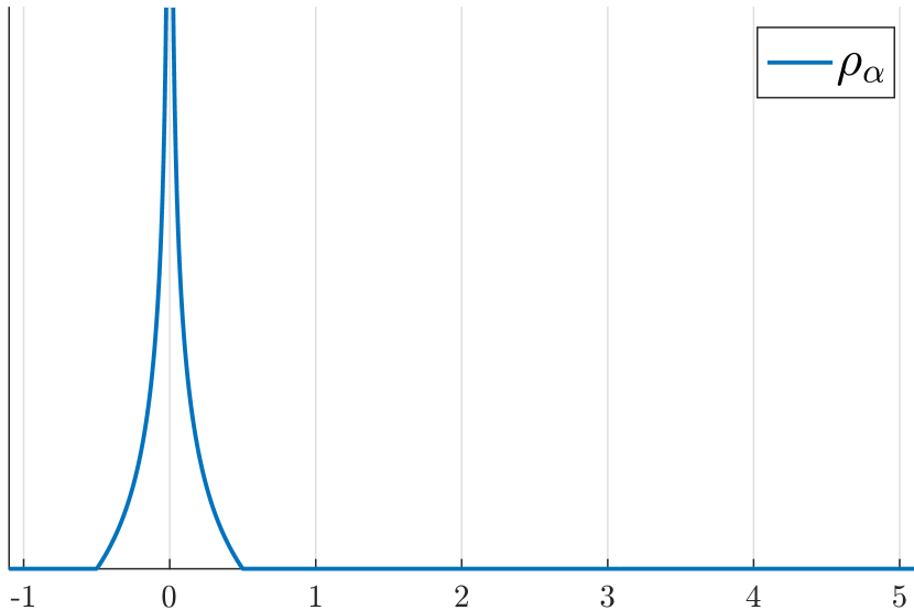
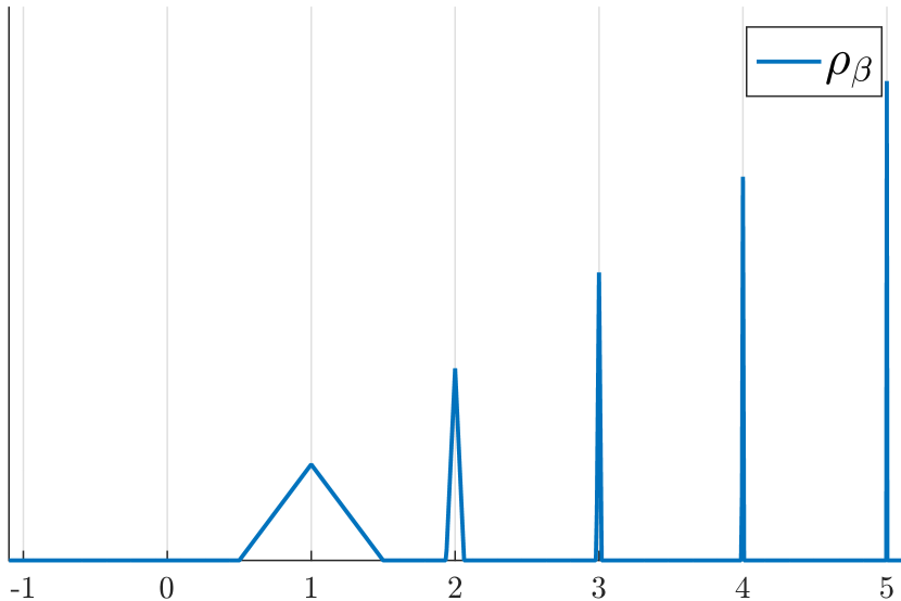
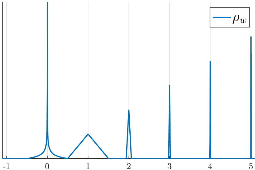
Figure 7.1: Choice of the probability densities $\rho_{\alpha}$, $\rho_{\beta}$ and $\rho_{w}$, $w=\nicefrac{{1}}{{10}}$, in Example 7.1. $u=0$ is an s:-mode of $\mu_{\alpha}$, while $\mu_{\beta}$ and $\mu_{w}$ have no (partial generalised) strong modes. However, $u=0$ is a w-mode of $\mu_{w}$ for any value of $w\in(0,1)$.

Example 7.1 (w-mode $\not\Rightarrow$ pgs-mode; gwa-mode $\not\Rightarrow$ pgs-mode; $[\forall\mathsf{cp}\forall\mathsf{cs}\exists\mathsf{as}\forall\mathsf{ns}]$-mode $\not\Rightarrow$ pgs-mode).

Consider the probability measures $\mu_{\alpha}$, $\mu_{\beta}$, $\mu_{w}\in\mathcal{P}(\mathbb{R})$ with PDFs given by

$$\rho_{\alpha}(x) \coloneqq 2\big{(}\left\lvert 2x\right\rvert^{-1/3}-1\big{)}\,\chi_{[-\nicefrac{{1}}{{2}},\nicefrac{{1}}{{2}}]}(x),$$

$$\rho_{\beta}(x) \coloneqq\frac{6}{\pi^{2}}\sum_{n\in\mathbb{N}}n\,t\big{(}n^{3}(x-n)\big{)}, t(x)\coloneqq(1+2x)\,\chi_{[-\nicefrac{{1}}{{2}},0]}(x)+(1-2x)\,\chi_{[0,\nicefrac{{1}}{{2}}]}(x),$$

$$\rho_{w}(x) \coloneqq w\,\rho_{\alpha}(x)+(1-w)\,\rho_{\beta}(x),$$

where $w\in(0,1)$ is a parameter. Figure 7.1 shows $\rho_{\alpha}$, $\rho_{\beta}$, and $\rho_{w}$ for $w=\nicefrac{{1}}{{10}}$. Since $\rho_{w}$ has its only singularity at $u=0$ and is continuous everywhere else, $u=0$ is the only w-mode of $\mu_{w}$:

$$\liminf_{r\to 0}\,\mathfrak{R}_{r}^{\mu_{w}}(u,v)\geqslant\liminf_{r\to 0}\frac{3(2r)^{2/3}}{4r\rho_{w}(v)}=\infty\geqslant 1\qquad\text{for any }v\neq u.$$

Similarly, $u=0$ is a gwa-mode and a $[\forall\mathsf{cp}\forall\mathsf{cs}\exists\mathsf{as}\forall\mathsf{ns}]$-mode of $\mu_{w}$. However, for $w=\nicefrac{{1}}{{10}}$, $u=0$ is not a pgs-mode of $\mu_{w}$: Defining $n(r)\coloneqq\lceil r^{-1/3}\rceil$, i.e. $n(r)^{-3}\leqslant r\leqslant(n(r)-1)^{-3}$, we have, for each $\mathsf{ns}\ (r_{n})_{n\in\mathbb{N}}$ and each $\mathsf{as}\ (u_{n})_{n\in\mathbb{N}}$ of $u=0$,

$$\liminf_{n\to\infty}\,\mathfrak{R}_{r_{n}}^{\mu_{w}}(u_{n},\sup) \leqslant\frac{w}{1-w}\limsup_{r\to 0}\frac{3(2r)^{2/3}-4r}{\mu_{\beta}(B_{n(r)^{-3}}(n(r)))}$$

$$\leqslant\frac{w}{1-w}\limsup_{r\to 0}\frac{3\cdot 2^{2/3}(n(r)-1)^{-2}}{\frac{6}{\pi^{2}}\,n(r)^{-2}}$$

$$=\frac{w}{1-w}\,\frac{\pi^{2}}{\sqrt[3]{2}}\approx 0.87<1.$$

In summary, for $w=\nicefrac{{1}}{{10}}$, $\mu_{w}$ has a w-mode that is a gwa-mode and a $[\forall\mathsf{cp}\forall\mathsf{cs}\exists\mathsf{as}\forall\mathsf{ns}]$-mode but not a pgs-mode.

The next example illustrates the difference between generalised and non-generalised modes:

Example 7.2 (gs-mode $\not\Rightarrow$ wp-mode; similar to Clason et al. 2019, Example 2.2).

Consider the probability measure $\mu\in\mathcal{P}(\mathbb{R})$ with pdf $\rho$ given by

$$\rho(x)\coloneqq\begin{cases}\lvert x\rvert&\text{for }x\in[-1,1],\\ 0&\text{otherwise.}\end{cases}$$

Clearly, the only points that could be wp-mode are $u=\pm 1$. However, for any $0<r<\nicefrac{{1}}{{3}}$,

$$\mu(B_{r}(\pm 1))<r<\tfrac{4}{3}r=\mu(B_{r}(\tfrac{2}{3}))$$

and hence $\mu$ has no wp-mode. On the other hand, for each $\mathsf{ns}\ (r_{n})_{n\in\mathbb{N}}$ (without loss of generality, we may assume $r_{n}<1$ for each $n\in\mathbb{N}$), we can choose the $\mathsf{as}\ u_{n}=1-r_{n}$ of $u=1$ to obtain

$$\mu(B_{r_{n}}(u_{n}))=2r_{n}(1-r_{n})=M_{r_{n}}^{\mu},$$

proving that $u=1$ is a gs-mode of $\mu$ (a similar computation can be performed for $u=-1$).

In the three examples below we will use the following terms and probability measures. Our construction is similar to the more general one of Lambley and Sullivan (2023).

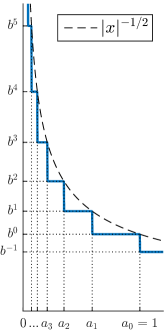
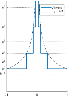
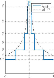
Figure 7.2: Quantities from Notation 7.3 for $b=\nicefrac{{13}}{{10}}$: left: choice of the values $a_{n}$, $n\in\mathbb{N}$; middle: density $\rho_{\textup{even}}$; right: density $\rho_{\textup{odd}}$.

Notation 7.3.

Let $b>1$ and, for $n\in\mathbb{Z}$, let $a_{n}\coloneqq b^{-2n}$, $r_{n}=a_{2n}=b^{-4n}$, $\tilde{r}_{n}=a_{2n+1}=b^{-4n-2}$ and $C=\frac{b^{2}+1}{2b}>1$. Further, define the finite measures (not probability measures) $\mu_{\textup{even}}$ and $\mu_{\textup{odd}}$ on $\mathbb{R}$ with Lebesgue densities

$$\rho_{\textup{even}}(x) \coloneqq\begin{cases}\sup\bigl{\{}b^{2n}\,\big{|}\,n\in\mathbb{Z},\,\lvert x\rvert^{1/2}\leqslant b^{-2n}\bigr{\}}&\text{for }x\in[-1,1],\\ 0&\text{otherwise},\end{cases}$$

$$\rho_{\textup{odd}}(x) \coloneqq\begin{cases}\sup\bigl{\{}b^{2n+1}\,\big{|}\,n\in\mathbb{Z},\,\lvert x\rvert^{1/2}\leqslant b^{-2n-1}\bigr{\}}&\text{for }x\in[-1,1],\\ 0&\text{otherwise},\end{cases}$$

illustrated in Figure 7.2. The measures $\mu_{\textup{even}}$ and $\mu_{\textup{odd}}$ are finite since $\rho_{\textup{even}}$ and $\rho_{\textup{odd}}$ are bounded by the function $f(x)=\lvert x\rvert^{-1/2}$ (with $f(0)\coloneqq\infty$) which is Lebesgue integrable on $[-1,1]$.

Proposition 7.4.

Using Notation 7.3, we have, for any $0<r<1$,

$$\frac{\mu_{\textup{even}}(B_{r_{n}}(0))}{\mu_{\textup{odd}}(B_{r_{n}}(0))}=C,\qquad\frac{\mu_{\textup{even}}(B_{\tilde{r}_{n}}(0))}{\mu_{\textup{odd}}(B_{\tilde{r}_{n}}(0))}=C^{-1},\qquad\frac{\mu_{\textup{even}}(B_{r}(0))}{\mu_{\textup{odd}}(B_{r}(0))}\in\left[C^{-1},C\right].$$

In particular, $\liminf_{r\to 0}\frac{\mu_{\textup{even}}(B_{r}(0))}{\mu_{\textup{odd}}(B_{r}(0))}=C^{-1}$ and $\limsup_{r\to 0}\frac{\mu_{\textup{even}}(B_{r}(0))}{\mu_{\textup{odd}}(B_{r}(0))}=C$.

Proof.

For any $n\in\mathbb{N}$ and $r\in[\tilde{r}_{n},r_{n}]$ we have:

$$\mu_{\textup{even}}(B_{r}(0)) =2rb^{2n}+\sum_{j\geqslant n+1}2a_{2j}(b^{2j}-b^{2j-2})=2rb^{2n}+2b^{-2n-2},$$

$$\mu_{\textup{odd}}(B_{r}(0)) =2rb^{2n-1}+\sum_{j\geqslant n}2a_{2j+1}(b^{2j+1}-b^{2j-1})=2rb^{2n-1}+b^{-2n-1}.$$

By Lemma A.4 the ratio $R(r)\coloneqq\frac{\mu_{\textup{even}}(B_{r}(0))}{\mu_{\textup{odd}}(B_{r}(0))}$ is strictly increasing in $r$ on each interval $[\tilde{r}_{n},r_{n}]$, $n\in\mathbb{N}$, and that its values on the boundary are $R(\tilde{r}_{n})=C^{-1}<1$ and $R(r_{n})=C>1$. A similar calculation shows that $R$ is strictly decreasing on every interval $[r_{n+1},\tilde{r}_{n}]$, $n\in\mathbb{N}$. ∎

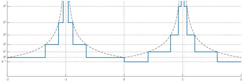
Figure 7.3: Choice of the density $\rho$ in Example 7.5 for $b=\nicefrac{{13}}{{10}}$ (before normalisation). As the radius decreases, $r\to 0$, the two points $u=+1$ and $v=-1$ ‘take turns’ in dominating the $r$-ball probability at the corresponding point; the ratio $\,\mathfrak{R}_{r}^{\mu}(-1,1)$ oscillates alternates between values either side of unity so that its limits superior and inferior are either side of unity. Hence, $u,v$ are neither gw-mode nor wag-modes of $\mu$, while they are ps-mode of $\mu$.

The following example illustrates the difference between partial and non-partial modes by considering the density $\rho(x)\propto\rho_{\textup{even}}(x+1)+\rho_{\textup{odd}}(x-1)$, illustrated in Figure 7.3. As $r\to 0$, the points $\pm 1$ take turns in being dominant in terms of their radius-$r$ ball probabilities. Therefore, the points $\pm 1$ cannot be non-partial modes (wg-modes), while, since partial modes allow for dominance only along a certain subsequence $r_{n}\to 0$, both are ps-mode. This example also illustrates how previous definitions of modes failed to satisfy the merging properties MP and rMP, while partial modes give hope for a remedy of this shortcoming. However, as Example 7.7 will show, partial modes also fail to fulfil MP and rMP.

Example 7.5 (ps-mode $\not\Rightarrow$ s-mode; ps-mode $\not\Rightarrow$ gw-mode; ps-mode $\not\Rightarrow$ wag-mode; certain non-partial modes satisfy neither MP nor rMP).

Using Notation 7.3, consider the probability measure $\mu\in\mathcal{P}(\mathbb{R})$ with pdf $\rho(x)\propto\rho_{\textup{even}}(x+1)+\rho_{\textup{odd}}(x-1)$, illustrated in Figure 7.3. By Proposition 7.4,

$$\,\mathfrak{R}_{r_{n}}^{\mu}(-1,+1)=C>1,\qquad\,\mathfrak{R}_{\tilde{r}_{n}}^{\mu}(-1,+1)=C^{-1}<1.$$

Hence, both $u_{A}=-1$ and $u_{B}=1$ are neither s-mode nor gw-mode nor wag-modes nor $[\forall\mathsf{cp}\exists\mathsf{as}\forall\mathsf{ns}]$-modes of $\mu$ (note that the constant $\mathsf{as}\ u_{n}=u_{A}$ of $u_{A}$ is optimal in terms of small ball probabilities, and similarly for $u_{B}$; and that it is sufficient to consider the two singularity points $u_{A}$ and $u_{B}$ since they clearly dominate every other point). However, both are ps:-modes of $\mu$, since, for the sequences $r_{n}$ (respectively $\tilde{r}_{n}$) we obtain

$$\lim_{n\to\infty}\,\mathfrak{R}_{r_{n}}^{\mu}(-1,\sup)=1,\qquad\lim_{n\to\infty}\,\mathfrak{R}_{\tilde{r}_{n}}^{\mu}(1,\sup)=1.$$

Further, if we choose $A=(-\infty,-\nicefrac{{1}}{{2}})$ and $B=(\nicefrac{{1}}{{2}},\infty)$, then $u_{A}$ and $u_{B}$ are $\textswab{s:}$-modes of $\mu|_{A}$ and $\mu|_{B}$, respectively, while, as we have just seen, $\mu|_{A\cup B}$ has no w-modes, gw-modes or wag-modes, which disproves both MP and rMP for all relevant non-partial modes; see Proposition 5.11.

Example 7.6 (counterexample to (Helin and Burger, 2015, Lemma 3); cf. Remark 3.5).

Using Notation 7.3, consider the probability measure $\mu$ on $\mathbb{R}$ with pdf $\rho(x)\propto\rho_{\textup{even}}(x+1)+C\rho_{\textup{odd}}(x-1)$. By Proposition 7.4,

$$\liminf_{r\to 0}\,\mathfrak{R}_{r}^{\mu}(-1,1)=C^{-2},\qquad\limsup_{r\to 0}\,\mathfrak{R}_{r}^{\mu}(-1,1)=1.$$

Hence, $u_{B}=1$ is a strong mode of $\mu$ (note again that it is sufficient to consider the two singularity points $u_{A}=-1$ and $u_{B}=1$), but not an $\mathbb{R}$-weak mode in the sense of Helin and Burger (2015, Definition 4), since the limit $\lim_{r\to 0}\,\mathfrak{R}_{r}^{\mu}(-1,1)$ fails to exist, providing a counterexample to Helin and Burger (2015, Lemma 3). It is, however, a (global) weak mode in the sense of our definition of weak modes (Definition 3.4), which ‘saves’ the implication that every s:-mode is a w-mode, cf. Remark 3.5.

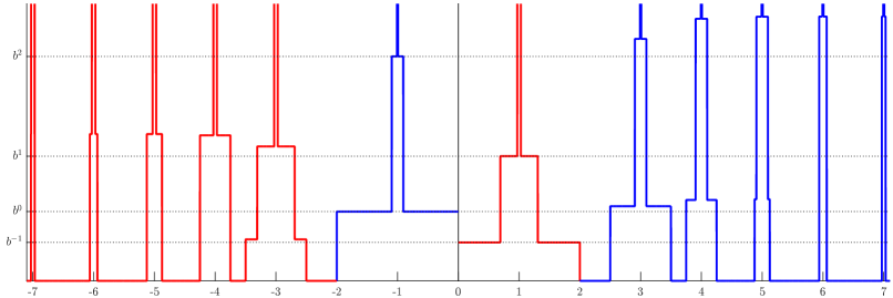
Figure 7.4: Choice of the density $\rho$ in Example 7.7 for $b=\nicefrac{{9}}{{5}}$ and $\beta=10$ (before normalisation). The parts in blue correspond to (restricted, scaled, shifted) versions of $\rho_{\textup{even}}$, while the parts in red correspond to (restricted, scaled, shifted) versions of $\rho_{\textup{odd}}$. While $u=-1$ dominates $u_{k}=-k-2$ for any $k\in\mathbb{N}$ with respect to the $\mathsf{ns}\ (r_{n})_{n\in\mathbb{N}}$ and is thereby a partial strong mode of $\mu|_{A}$ with $A=(-\infty,\nicefrac{{1}}{{2}})$, it is dominated by $v_{k}=k+2$ for each $k\in\mathbb{N}$ with respect to every $\mathsf{ns}\ (r_{n}^{\prime})$. It is therefore not a partial mode of $\mu$ for all definitions of partial modes in this paper (i.e. definitions listed in Table 6.1 that include the $\exists\mathsf{ns}$ quantifier). A similar argument works for $v=1$, $(\tilde{r}_{n})_{n\in\mathbb{N}}$ and $\mu|_{B}$ with $B=(-\nicefrac{{1}}{{2}},\infty)$. Note that no $u_{k}$ can be a partial mode of $\mu$, since it is strictly dominated by its neighbour $u_{k+1}$ with respect to every $\mathsf{ns}\ (r_{n}^{\prime})_{n\in\mathbb{N}}$, and similarly for $v_{k}$. Thus, $\mu$ has no partial modes, showing that all definitions of partial modes violate both MP and rMP.

As illustrated by Example 7.5, partial modes give hope to remedy the shortcoming of conventional definitions of modes to satisfy the merging properties MP and rMP. However, the following slightly more sophisticated example shows that this is not the case:

Example 7.7 (certain partial modes satisfy neither MP nor rMP).

Using Notation 7.3, let $\beta>1$ such that $C-\beta^{-1}>1$, let $I_{k}\coloneqq(-2^{-k},2^{-k})$, $u_{k}=-k-2$ and $v_{k}=k+2$ for $k\in\mathbb{N}$. Define the probability measure $\mu\in\mathcal{P}(\mathbb{R})$ by the pdf

$$\rho(x)\propto\rho_{\textup{even}}(x+1)+\rho_{\textup{odd}}(x-1)+\sum_{k=1}^{\infty}(C-\beta^{-k})\left(\rho_{\textup{even}}\big{|}_{I_{k}}(x-v_{k})+\rho_{\textup{odd}}\big{|}_{I_{k}}(x-u_{k})\right).$$

Note that, in the following, it is sufficient to consider only the singularity points of $\rho$ for generalised (partial) strong and generalised (partial) weak modes, since no other points have a chance of being modes. Further, it is sufficient to consider constant $\mathsf{as}\ x_{n}=x$ of $x$, since these are optimal in terms of small ball probabilities for all singularities of $\rho$.

Now let $A=(-\infty,-\nicefrac{{1}}{{2}})$ and $B=(\nicefrac{{1}}{{2}},\infty)$. Then $u_{A}=-1$ is a ps-mode of $\mu_{A}$ since, for any $k\in\mathbb{N}$ and sufficiently large $n\in\mathbb{N}$, Proposition 7.4 implies

$$\,\mathfrak{R}_{r_{n}}^{\mu|_{A}}(u_{A},\sup)=\min\left(1,\frac{\mu(B_{r_{n}}(u_{A}))}{\sup_{k\in\mathbb{N}}\mu(B_{r_{n}}(u_{k}))}\right)=\min\left(1,\frac{\mu_{\textup{even}}(B_{r_{n}}(0))}{\mu_{\textup{odd}}(B_{r_{n}}(0))\sup_{k\in\mathbb{N}}(C-\beta^{-k})}\right)=1.$$

However, each $u_{k}$ is strictly dominated by its neighbour $u_{k+1}$ in terms of small ball probabilities for each $\mathsf{ns}\ (r_{n}^{\prime})_{n\in\mathbb{N}}$, since, for sufficiently small $r>0$,

$$\,\mathfrak{R}_{r}^{\mu|_{A}}(u_{k+1},u_{k})=\frac{(C-\beta^{-k-1})\mu_{\textup{odd}}(B_{r}(0))}{(C-\beta^{-k})\mu_{\textup{odd}}(B_{r}(0))}=\frac{C-\beta^{-k-1}}{C-\beta^{-k}}>1.$$

Hence, for each $k\in\mathbb{N}$, $u_{k}$ is not even a wapg-mode of $\mu_{A}$ or $\mu|_{A\cup B}$ (and hence neither a wpag-mode nor a wgap-mode). Similar statements for $\mu_{B}$ and $u_{B}=1$ can be derived in the same way. Further, $u_{A}=-1$ is strictly dominated by each $v_{k}$, $k\in\mathbb{N}$, for each $\mathsf{ns}\ (r_{n}^{\prime})_{n\in\mathbb{N}}$, since, for any $0<r<\nicefrac{{1}}{{2}}$,

$$\,\mathfrak{R}_{r}^{\mu|_{A}}(v_{k},u)=\frac{(C-\beta^{-k})\mu_{\textup{even}}(B_{r}(0))}{\mu_{\textup{even}}(B_{r}(0))}=C-\beta^{-k}>1.$$

A similar argument holds for $u_{B}=1$. Hence, $u_{A}$ and $u_{B}$ are the only ps-mode of $\mu_{A}$ and $\mu_{B}$, respectively, while $\mu|_{A\cup B}$ has no wpag-mode or wgap-mode, violating MP and rMP for a large class of partial modes, cf. Proposition 5.11.

The following example is very similar to Example 7.5 — but with three singularities instead of just two, and a fourth that is a ‘mean’ of the others — and shows that the order of the quantifiers w and p is significant. Since the line of argument is hopefully becoming familiar, we do not spell out all the details.

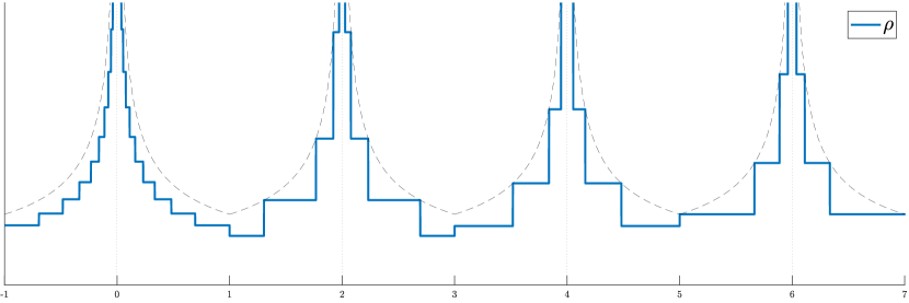
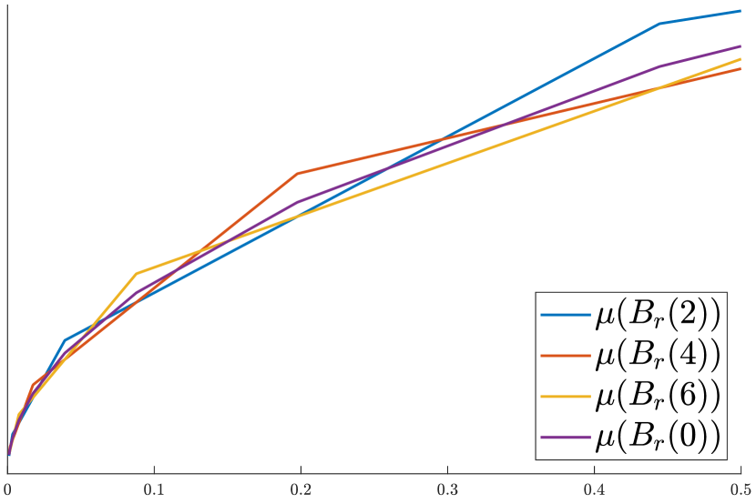
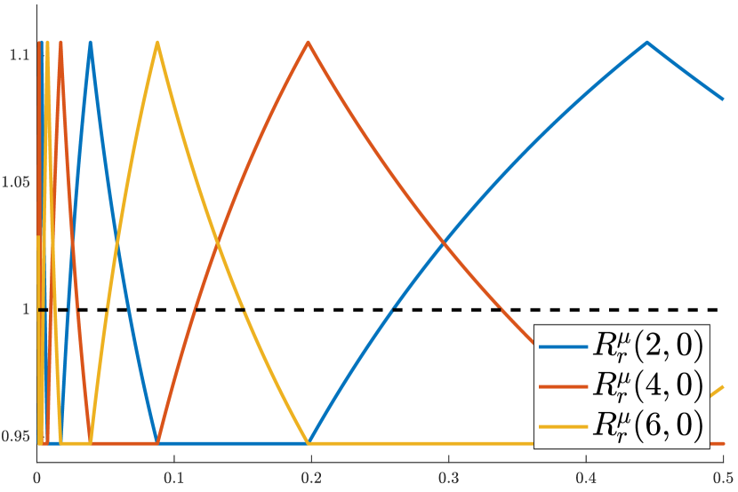
Figure 7.5: Illustration of Example 7.8. Top: The Lebesgue density $\rho$ of $\mu$ for $b=\nicefrac{{6}}{{5}}$. Bottom: The ‘radial cumulative distribution function’ $\mu(B_{r}(x))$ and ratios $\,\mathfrak{R}_{r}^{\mu}(x,0)$ as functions of $r$ for several critical values of $x$ and $b=\nicefrac{{3}}{{2}}$.
As $r\to 0$, the singularities at $x=2$, $4$, and $6$ take turns in dominating the other ones. As a result, the ‘mean’ singularity in $u=0$ dominates each of the other singularities for certain null sequences, but there is no $\mathsf{ns}$ for which it dominates the other points simultaneously.

Example 7.8 (wp-mode $\not\Rightarrow$ pw-mode; gwpa-mode $\not\Rightarrow$ pwag-mode).

Let $b>1$ and $\mu_{k}$, $k=1,2,3$, be finite measures on $\mathbb{R}$ given by their Lebesgue densities

$$\rho_{k}(x) \coloneqq\begin{cases}\sup\bigl{\{}b^{3n+k}\,\big{|}\,n\in\mathbb{Z},\,\lvert x\rvert^{1/2}\leqslant b^{-3n-k}\bigr{\}}&\text{for }x\in[-1,1],\\ 0&\text{otherwise}.\end{cases}$$

Consider the measure $$\mu$$ given by its Lebesgue density

$$\rho(x) \coloneqq\sum_{k=1}^{3}\tfrac{1}{3}\rho_{k}(x)+\rho_{k}(x-2k).$$

For simplicity, we will work with the unnormalised density $\rho$, illustrated in Figure 7.5, instead of the corresponding normalised pdf, which clearly has no influence on the small ball probability ratios. We will argue that $u=0$ is a wp-mode but not a pw-mode of $\mu$. The reason is that, for each $\mathsf{cp}\ v\in\mathbb{R}$, there exists a $\mathsf{ns}$ for which $u=0$ dominates $v$, but there is no $\mathsf{ns}$ that works for all $\mathsf{cp}$ simultaneously. For the same reason, $u=0$ is a gwpa-mode, but not a pwag-mode of $\mu$.

Analogously to the calculations in the proof of Proposition 7.4, we derive, for any $k=1,2,3$ and $b^{-3(n+1)-k}<r^{1/2}\leqslant b^{-3n-k}$,

$$\mu(B_{r}(2k))=2rb^{3n+k}+\sum_{j\geqslant n+1}2b^{-6j-2k}\big{(}b^{3j+k}-b^{3(j-1)+k}\big{)}=2rb^{3n+k}+2b^{-3n-3-k},$$

showing that $u=0$ dominates $u^{(k)}=2k$ for the $\mathsf{ns}\ r_{n}^{(k)}=b^{-3n-k-1}$, $k=1,2,3$, respectively, as illustrated in Figure 7.5 (bottom right). However, no $\mathsf{ns}$ works for all the three $u^{(k)}$ simultaneously. Consequently, $u=0$ is a wp-mode, a gwpa-mode and an $[\forall\mathsf{as}\forall\mathsf{cp}\exists\mathsf{ns}]$-mode (note that the constant $\mathsf{as}$ of all singularities are clearly ‘optimal’), but neither a pw-mode nor a pwag-mode nor a $[\forall\mathsf{as}\exists\mathsf{ns}\forall\mathsf{cp}]$-mode.

In order to show that the quantifiers w and g are not interchangeable, the next example modifies the previous one by making the singularities ‘one-sided’ (cf. Figure 7.6) such that approximating sequences other than $u_{n}=u$ and $v_{n}=v$ are actually significant. Again, since the line of argument is similar to previous ones, we do not spell out all the details.

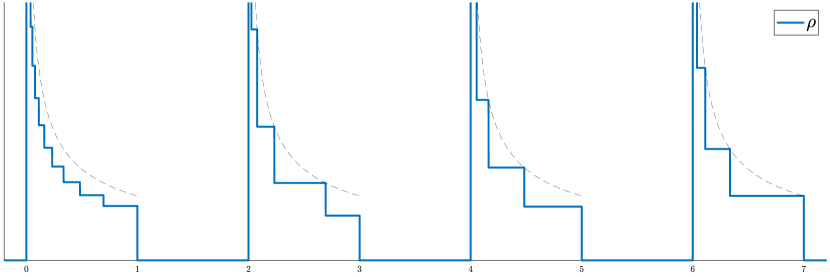
Figure 7.6: Illustration of the Lebesgue density $\rho$ in Example 7.9.

Example 7.9 (wpga-mode $\not\Rightarrow$ gwap-mode; wpga-mode $\not\Rightarrow$ pwag-mode).

Let $1<b\leqslant\nicefrac{{3}}{{2}}$. Further, define the finite measures $\mu_{k}$, $k=1,2,3$, on $\mathbb{R}$ by their Lebesgue densities

$$\rho_{k}(x) \coloneqq\begin{cases}\sup\bigl{\{}b^{3n+k}\,\big{|}\,n\in\mathbb{Z},\,\lvert x\rvert^{1/2}\leqslant b^{-3n-k}\bigr{\}}&\text{for }x\in[0,1],\\ 0&\text{otherwise},\end{cases}$$

as well as the measure $$\mu$$ by its density

$$\rho(x) \coloneqq\sum_{k=1}^{3}\tfrac{1}{3}\rho_{k}(x)+\rho_{k}(x-2k).$$

For simplicity, we will work with the unnormalised density $\rho$, illustrated in Figure 7.6, instead of the corresponding normalised pdf, which clearly has no influence on the small ball probability ratios. We argue that $u=0$ is a wpga-mode but neither a gwap-mode, nor a pwag-mode of $\mu$. The reason is that, for each $\mathsf{cp}\ v\in\mathbb{R}$, there exists a $\mathsf{ns}\ (r_{n})_{n\in\mathbb{N}}$ and an $\mathsf{as}\ (u_{n})_{n\in\mathbb{N}}$ of $u$, namely $u_{n}\coloneqq r_{n}$, such that $(u_{n})_{n\in\mathbb{N}}$ dominates each $\mathsf{cs}\ (v_{n})_{n\in\mathbb{N}}$ of $v$ (the critical one being $v+r_{n}$), but there is no $\mathsf{ns}$ of $u$ (with corresponding $\mathsf{as}$ $u_{n}\coloneqq r_{n}$) that works for all $\mathsf{cp}$ simultaneously. The calculations are similar to Example 7.8 and are therefore left to the reader.

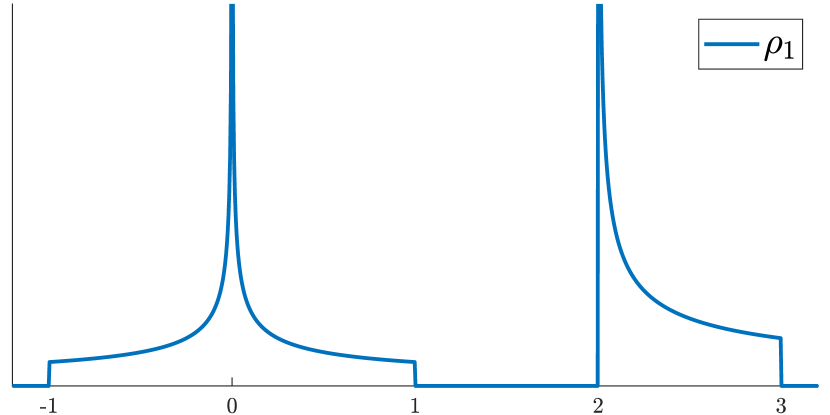
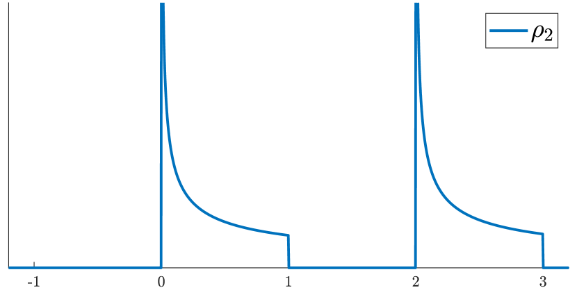
Figure 7.7: Illustration of the densities $\rho_{1}$ and $\rho_{2}$ in Example 7.10.

Example 7.10 (w $\not\Rightarrow$ wpag; violation of SP and CP).

Consider the probability measures $\mu_{0},\mu_{1},\mu_{2}\in\mathcal{P}(\mathbb{R})$ with probability densities

$$\rho_{0}(x) =\begin{cases}\tfrac{1}{2}\lvert x\rvert^{-1/2}&\text{if }x\in(0,1),\\ 0&\text{otherwise},\end{cases}$$

$$\rho_{1}(x) =\alpha\rho_{0}(x)+\alpha\rho_{0}(-x)+(1-2\alpha)\rho_{0}(x-2), 0\leqslant\alpha\leqslant\nicefrac{{1}}{{2}},$$

$$\rho_{2}(x) =\beta\rho_{0}(x)+(1-\beta)\rho_{0}(x-2), \beta=0.49,$$

respectively. $\rho_{1}$ and $\rho_{2}$ are illustrated in Figure 7.7. Note that, for $r<\nicefrac{{1}}{{2}}$ and $-r\leqslant t\leqslant r$, $\mu_{0}(B_{r}(t))=\sqrt{r+t}$, in particular,

$$\mu_{0}(B_{r}(0))=\sqrt{r},\qquad\mu_{0}(B_{r}(r))=\sqrt{2r},\qquad\mu_{0}(B_{r}(-r/2))=\sqrt{r/2}.$$ (7.1)

Hence it is crucial which of the points $u$ and $v$ in the definition of modes is/are allowed an approximating sequence:

1. For the measure $\mu_{1}$ with $\alpha=\nicefrac{{1}}{{4}}$ the points $u=0$ and $v=2$ clearly dominate every other point in terms of small ball probabilities (as they are the only singularities), so it is sufficient to compare these two points. Since $\,\mathfrak{R}_{r}^{\mu_{1}}(0,2)=1$ for each $r>0$, both are w-mode of $\mu_{1}$. However, for $v=2$ and for each $\mathsf{ns}\ (r_{n})_{n\in\mathbb{N}}$ (without loss of generality we assume $r_{n}<1$ for each $n\in\mathbb{N}$) and each $\mathsf{as}\ (u_{n})_{n\in\mathbb{N}}$ of $u=0$ (note that the constant $\mathsf{as}\ u_{n}=0$ of $u=0$ is always ‘optimal’), the $\mathsf{cs}\ v_{n}=2+r_{n}$ of $v=2$ satisfies $\,\mathfrak{R}_{r_{n}}^{\mu_{1}}(u_{n},v_{n})\leqslant\nicefrac{{1}}{{\sqrt{2}}}<1$. Hence, $u=0$ is a w-mode, but not a wpag-mode of $\mu_{1}$.

2. For the measure $\mu_{0}$ and certain mode types in Definition 4.2, $u=0$ dominates every other $\mathsf{cp}\ v\neq u$ but fails to dominate itself, excluding such definitions by SP, as listed in Proposition 5.3.

3. If CP holds and $u=0$ is a mode of $\mu_{0}$, then $u=2$ must be the only mode of $\mu_{2}$. This excludes a large number of mode definitions from Definition 4.2, listed in Proposition 5.4.

8 Conclusion

Defining a mode for a probability measure without a continuous Lebesgue PDF, e.g. in infinite-dimensional Hilbert and Banach spaces or other metric spaces, is neither trivial nor unambiguous, and still a topic of current research. This manuscript introduced a structured way of defining modes that incorporates all previous definitions as well as over 100 alternatives that are at least grammatically correct. In order to filter out those definitions that are actually meaningful, we introduced several common-sense axioms that modes ought to satisfy — such as the correct identification of modes for measures that possess atoms or a continuous Lebesgue PDF, as well as proper behaviour under copying, shifting and taking averages of probability measures on normed spaces. Excluding all definitions that violate these axioms for $X=\mathbb{R}$ — except for the challenging ‘merging property’ (MP) — leaves 17 distinct meaningful definitions for a mode, some rather exotic, but none objectively inferior to another at this point.

We established causal relations among these definitions and presented a large number of illuminating examples and counterexamples, which hopefully will shape the future development of the theory on modes and MAP estimators. In particular, we have realised a new ‘exotic’ mode, the $[\forall\mathsf{cp}\forall\mathsf{cs}\exists\mathsf{as}\forall\mathsf{ns}]$-mode, located strictly between the strong mode of Dashti et al. (2013) and the weak mode of Helin and Burger (2015) and Ayanbayev et al. (2022). Note that the probability measures in all our examples could be constructed on $X=\mathbb{R}$ and possess a (possibly discontinuous) PDF.

One of our proposed axioms, the MP, highlights a crucial shortcoming of all extant definitions of modes: for open sets $A,B\subseteq X$ it can happen that both $\mu|_{A}$ and $\mu|_{B}$ possess a mode while $\mu|_{A\cup B}$ has no modes, which runs counter to our intuition about modes. Our own attempt to fix this issue led to the definition of ‘partial modes’, which, unfortunately, also do not satisfy the MP. In fact, none of the 17 meaningful definitions that we identified satisfies the MP, leaving the fully satisfactory definition of modes and MAP estimators as an open problem that deserves further research.

Appendix A Supporting technical results

Lemma A.1.

Let $(X,d)$ be a separable metric space, $\mu\in\mathcal{P}(X)$, $u\in\operatorname{supp}(\mu)$ and let $(\Delta_{n})_{n\in\mathbb{N}}$ be any null sequence. Then there exist null sequences $(r_{n})_{n\in\mathbb{N}}$, $(\tilde{r}_{n})_{n\in\mathbb{N}}$ and $(\varepsilon_{n})_{n\in\mathbb{N}}$ such that

$$\mu(B_{r_{n}-\Delta_{n}}(u))\geqslant(1-\varepsilon_{n})\,\mu(B_{r_{n}}(u)),\qquad\mu(B_{\tilde{r}_{n}+\Delta_{n}}(u))\leqslant(1+\varepsilon_{n})\,\mu(B_{\tilde{r}_{n}}(u)).$$

Proof.

We will first show that there exist a null sequences $(s_{k})_{k\in\mathbb{N}}$ and $(\tilde{s}_{k})_{k\in\mathbb{N}}$ and a strictly increasing sequence $(n_{k})_{k\in\mathbb{N}}$ such that, for each $n\geqslant n_{k}$,

$$\mu\bigl{(}B_{s_{k}}(u)\setminus B_{s_{k}-\Delta_{n}}(u)\bigr{)}\leqslant k^{-1}\mu(B_{s_{k}}(u)),\quad\mu\bigl{(}B_{\tilde{s}_{k}+\Delta_{n}}(u)\setminus B_{\tilde{s}_{k}}(u)\bigr{)}\leqslant k^{-1}\mu(B_{\tilde{s}_{k}}(u)).$$ (A.1)

Since $\mu$ is a finite measure, this holds trivially for $k=1$ with $s_{1}=1$ and $n_{1}=1$ and sufficiently large $\tilde{s}_{1}>0$, while for $k\geqslant 2$ we can construct $s_{k}$ and $n_{k}$ recursively: Set $\hat{s}=s_{k-1}/2$, $\check{s}=s_{k-1}/4$, $Q=\mu(B_{\hat{s}}(u))/\mu(B_{\check{s}}(u))\geqslant 1$, $J=\lceil{Qk}\rceil$ and $\delta=(\hat{s}-\check{s})/J>0$. Since the rings $A_{j}\coloneqq B_{\check{s}+j\delta}(u)\setminus B_{\check{s}+(j-1)\delta}(u)\subseteq B_{\hat{s}}(u)$, $j=1,\dots,J$, are disjoint,

$$\sum_{j=1}^{J}\mu(A_{j})\leqslant\mu(B_{\hat{s}}(u))=Q\,\mu(B_{\check{s}}(u)).$$

Hence, there exists $j^{\ast}\in\{1,\dots,J\}$ such that $\mu(A_{j^{\ast}})\leqslant J^{-1}Q\,\mu(B_{\check{s}}(u))$. Choose $s_{k}\coloneqq\check{s}+j^{\ast}\delta$ and $\tilde{s}_{k}\coloneqq\check{s}+(j^{\ast}-1)\delta$. Further, since $u_{n}\to u$ as $n\to\infty$, there exists $n_{k}\geqslant n_{k-1}$ such that, for each $n\geqslant n_{k}$, $\Delta_{n}\leqslant\delta$. Since $J^{-1}Q\leqslant k^{-1}$ and $B_{s_{k}}(u)\setminus B_{s_{k}-\Delta_{n}}(u)\subseteq A_{j^{\ast}}$ as well as $B_{\tilde{s}_{k}+\Delta_{n}}(u)\setminus B_{\tilde{s}_{k}}(u)\subseteq A_{j^{\ast}}$ for $n\geqslant n_{k}$, this proves (A.1), (note that $(s_{k})_{k\in\mathbb{N}}$ and $(\tilde{s}_{k})_{k\in\mathbb{N}}$ are null sequences since $s_{k}\leqslant s_{k-1}/2$, $\tilde{s}_{k}\leqslant s_{k-1}/2$).

Now, choosing $r_{n}=s_{k}$, $\tilde{r}_{n}=\tilde{s}_{k}$ and $\varepsilon_{n}=k^{-1}$ whenever $n_{k}\leqslant n<n_{k+1}$ for some (unique) $k\in\mathbb{N}$, the above construction yields, for each $n\in\mathbb{N}$,

$$\mu\bigl{(}B_{r_{n}}(u)\setminus B_{r_{n}-\Delta_{n}}(u)\bigr{)} \leqslant\varepsilon_{n}\mu(B_{r_{n}}(u))\text{ and}$$

$$\mu\bigl{(}B_{\tilde{r}_{n}+\Delta_{n}}(u)\setminus B_{\tilde{r}_{n}}(u)\bigr{)} \leqslant\varepsilon_{n}\mu(B_{\tilde{r}_{n}}(u)).$$

Since

$$B_{r_{n}}(u) =B_{r_{n}-\Delta_{n}}(u)\uplus\bigl{(}B_{r_{n}}(u)\setminus B_{r_{n}-\Delta_{n}}(u)\bigr{)}\text{ and}$$

$$B_{\tilde{r}_{n}+\Delta_{n}}(u) =B_{\tilde{r}_{n}}(u)\uplus\bigl{(}B_{\tilde{r}_{n}+\Delta_{n}}(u)\setminus B_{\tilde{r}_{n}}(u)\bigr{)},$$

this proves the claim. ∎

Lemma A.2.

Let $\mu\in\mathcal{P}(X)$. Then, for each $x\in X$ and $s>0$,

$$\lim_{r\nearrow s}\mu(B_{r}(x))=\mu(B_{s}(x)),\qquad\lim_{r\nearrow s}M_{r}^{\mu}=M_{s}^{\mu}.$$

Proof.

Since $B_{r}(x)$ is monotonically increasing in $r$ with $B_{s}(x)=\bigcup_{r<s}B_{r}(x)$, the first identity follows directly from the continuity of measures. Now assume that the second identity does not hold, i.e. there exists $\varepsilon>0$ such that, for each $r<s$, $M_{r}^{\mu}\leqslant M_{s}^{\mu}-\varepsilon$. By definition of the supremum, there exists $x_{\ast}\in X$ such that $\mu(B_{s}(x_{\ast}))>M_{s}^{\mu}-\varepsilon$. Hence, using the first identity, we obtain the contradiction

$$M_{s}^{\mu}-\varepsilon\geqslant\limsup_{r\nearrow s}M_{r}^{\mu}\geqslant\lim_{r\nearrow s}\mu(B_{r}(x_{\ast}))=\mu(B_{s}(x_{\ast}))>M_{s}^{\mu}-\varepsilon.\qed$$

Lemma A.3.

Let $\mu\in\mathcal{P}(X)$. Then, for each $r>0$, the map $x\mapsto\mu(B_{r}(x))$ is lower semicontinuous on $X$, i.e. $\liminf_{k\to\infty}\mu(B_{r}(x_{k}))\geqslant\mu(B_{r}(x))$ for any convergent sequence $(x_{k})_{k\in\mathbb{N}}$ in $X$ with limit $x\in X$.

Proof.

See e.g. Lambley and Sullivan (2023, SM1.1). ∎

Lemma A.4.

Let $a,b,c,d>0$ and $f\colon(0,\infty)\to\mathbb{R}$ be given by $f(x)\coloneqq\frac{ax+b}{cx+d}$. Then $f$ is strictly monotonically increasing if and only if $ad>bc$.

Proof.

Note that $f$ is well defined, as its domain has been chosen to exclude the singularity at $x=-\tfrac{d}{c}<0$. The derivative of $f$,

$$f^{\prime}(x)=\frac{a(cx+d)-c(ax+b)}{(cx+d)^{2}}=\frac{ad-bc}{(cx+d)^{2}},$$

is strictly positive for arbitrary $x\in(0,\infty)$ if and only if $ad-bc>0$. ∎

Appendix B Further plausible axioms for modes

Here we briefly sketch out some additional axioms or properties that one might require a ‘meaningful’ definition of a mode to satisfy. The first two have a geometrical flavour, asking that modes behave well under simple linear transformations of the parameter space.

Definition B.1.

Let $X$ be a separable normed space. We say that a mode map $\mathfrak{M}\colon\mathcal{P}(X)\to 2^{X}$ satisfies

1. the homothety invariance property (HIP) if, for any $\mu\in\mathcal{P}(X)$, $b\in X$, and $s>0$,

   $$\mathfrak{M}(\mu(s^{-1}(\mathchoice{\mathbin{\vbox{\hbox{\scalebox{0.5}{$\;\displaystyle\bullet\;$}}}}}{\mathbin{\vbox{\hbox{\scalebox{0.5}{$\;\textstyle\bullet\;$}}}}}{\mathbin{\vbox{\hbox{\scalebox{0.5}{$\;\scriptstyle\bullet\;$}}}}}{\mathbin{\vbox{\hbox{\scalebox{0.5}{$\;\scriptscriptstyle\bullet\;$}}}}}-b)))=b+s\,\mathfrak{M}(\mu);$$

2. the affine invariance property (AIP) if $X=\mathbb{R}^{d}$ and, for any $\mu\in\mathcal{P}(X)$, $b\in X$, and invertible $A\in\mathbb{R}^{d\times d}$,

   $$\mathfrak{M}(\mu(A^{-1}(\mathchoice{\mathbin{\vbox{\hbox{\scalebox{0.5}{$\;\displaystyle\bullet\;$}}}}}{\mathbin{\vbox{\hbox{\scalebox{0.5}{$\;\textstyle\bullet\;$}}}}}{\mathbin{\vbox{\hbox{\scalebox{0.5}{$\;\scriptstyle\bullet\;$}}}}}{\mathbin{\vbox{\hbox{\scalebox{0.5}{$\;\scriptscriptstyle\bullet\;$}}}}}-b)))=b+A\,\mathfrak{M}(\mu);$$

HIP holds trivially for all definitions in Table 6.1, since they rely on small ball probabilities. Therefore, in order to avoid any distractions, we did not state these properties in Definition 5.1. AIP, on the other hand, cannot be expected to hold for modes defined via small ball probabilities, since these notions depend crucially on the chosen metric, which is modified non-trivially by scaling with an invertible matrix, in particular under rotation (Lie and Sullivan, 2018, Example 5.6). For this reason we did not study this property here.

Another attractive property arises naturally in the context of Bayesian inverse problems:

Definition B.2.

Let $X$ be a separable metric space. We say that a mode map $\mathfrak{M}\colon\mathcal{P}(X)\to 2^{X}$ satisfies the reweighting property (RP) if, for any $\mu,\nu\in\mathcal{P}(X)$ with $\nu\ll\mu$, the existence of a mode of $\mu$ implies the existence of a mode of $\nu$, i.e. $\mathfrak{M}(\mu)\neq\varnothing\implies\mathfrak{M}(\nu)\neq\varnothing$.

RP states that — for posteriors that are absolutely continuous with respect to the prior — the existence of a prior mode implies the existence of a posterior mode, i.e. of a MAP estimator; see e.g. Dashti et al. (2013), Klebanov and Wacker (2023), and Lambley (2023) for treatments of Gaussian priors. To make this an effective definition, one would also impose further restrictions on the Radon–Nikodym derivative of $\nu$ with respect to $\mu$ which are typical in the context of Bayesian inference; see e.g. (Stuart, 2010, Section 2, Assumption 2.6). A thorough study of mode maps satisfying RP is beyond the scope of this paper.

Finally, one could consider a formal restriction that $\mathfrak{M}(\mu)$ depends on $\mu$ only through small ball probabilities $\mu(B_{r}(x))$ in the limit as $r\to 0$:

Definition B.3.

Let $X$ be a separable metric space. We say that a mode map $\mathfrak{M}\colon\mathcal{P}(X)\to 2^{X}$ satisfies the small balls property (SBP) if, whenever $\mu,\nu\in\mathcal{P}(X)$ admit $R>0$ such that

$$\mu(B_{r}(x))=\nu(B_{r}(x))\quad\text{for all $x\in X$ and $0<r<R$,}$$

it follows that $\mathfrak{M}(\mu)=\mathfrak{M}(\nu)$.

Clearly, all mode definitions covered in this paper satisfy this property since they are directly defined through the probability masses of (infinitesimally) small balls, cf. Definition 4.2.

Note that the SBP is connected to the well-known question of whether each measure $\mu\in\mathcal{P}(X)$ is uniquely determined by its values on balls. While this is not the case for metric spaces (Davies, 1971), it has been shown for separable Banach spaces by Preiss and Tišer (1991). However, the determination of $\mu$ by its values on small balls is an open problem. As mentioned by Preiss and Tišer (1991, final remark), their proof can be generalised to large balls, but not to small balls.

Appendix C Definition of the ball mass ratio

The ratio $\,\mathfrak{R}_{r}^{\mu}(u,v)$ in (2.1) was defined to be $1$ whenever $\mu(B_{r}(u))=\mu(B_{r}(v))=0$. The reasoning behind this choice is that $u$ and $v$ are equally dominant in this case. However, one might also argue that a ball having zero mass should not dominate any other point and use the alternative definition $\nicefrac{{0}}{{0}}\coloneqq 0$.

It turns out that there are no major axiomatic reasons to insist upon $\nicefrac{{0}}{{0}}\coloneqq 0$ over $\nicefrac{{0}}{{0}}\coloneqq 1$, but a few points would change, and in the interests of objectivity we summarise the situation under the alternative definition $\nicefrac{{0}}{{0}}\coloneqq 0$.

• $[\forall\mathsf{cp}\exists\mathsf{cs}\forall\mathsf{as}\exists\mathsf{ns}]$-modes would no longer violate CP (and also satisfy LP, AP, and SP) and would therefore be added to Table 6.1. In this case, each $[\forall\mathsf{as}\forall\mathsf{cp}\exists\mathsf{ns}]$-mode would clearly be a $[\forall\mathsf{cp}\exists\mathsf{cs}\forall\mathsf{as}\exists\mathsf{ns}]$-mode, but the other direction would not hold. Indeed, for the measure $\mu_{1}$ in Example 7.10 with $\alpha=\nicefrac{{1}}{{8}}$ the point $u=0$ is not a $[\forall\mathsf{as}\forall\mathsf{cp}\exists\mathsf{ns}]$-mode, since it fails to dominate $v=2$ (for the $\mathsf{as}$ $u_{n}=u$ of $u$), but it is a $[\forall\mathsf{cp}\exists\mathsf{cs}\forall\mathsf{as}\exists\mathsf{ns}]$-mode — for the critical $\mathsf{cp}$ $v=2$, simply choose the $\mathsf{as}$ $v_{n}\coloneqq 2-n^{-1}$ of $v$ and the $\mathsf{ns}$ $r_{n}\coloneqq n^{-1}$, leading to $\,\mathfrak{R}_{r_{n}}^{\mu_{1}}(u_{n},v_{n})=\infty$ (for sufficiently large $n\in\mathbb{N}$), no matter how the $\mathsf{as}$ $(u_{n})_{n\in\mathbb{N}}$ of $u$ is chosen.

• The proof of Proposition 5.2 would be simpler, while the proof of Proposition 5.6 would be slightly harder. More precisely, the choice of the $\mathsf{as}$ in the proof of Proposition 5.6(b) as being identical to the $\mathsf{cs}$ would no longer work and would have to be replaced by the $\mathsf{as}$ $(u_{n})_{n\in\mathbb{N}}$ of $u$ given by $u_{n}=v_{n}$ whenever $\mu(B_{r_{n}}(v_{n}))\neq 0$ and $u_{n}=u$ otherwise (noting that $\mu(B_{r}(u))=0$ for any $r>0$ would contradict it being a mode); and this argument would be inapplicable for $[\forall\mathsf{cp}\forall\mathsf{cs}\exists\mathsf{as}\forall\mathsf{ns}]$-modes; despite our best efforts, we do not have a valid proof strategy for this case, resulting in an unresolved instance of SP in Table 6.1.

Appendix D Enumeration of all grammatically correct mode definitions

The following Appendix D enumerates all 282 possible definitions of a mode that are ‘grammatically correct’ in the sense of satisfying Definition 4.2. Appendix D aims to be obviously comprehensive more than to be readable per se, which is why this information has been relegated to an appendix. It is the role of Table 6.1 and Figure 6.1 in the main text to present the final list of 17 ‘meaningful’ mode definitions in aesthetically pleasing ways.

The first column of Appendix D gives the index $1\leqslant i\leqslant 282$ of each grammatically correct mode definition: the indexing results from using the standard Python 3.10.8 function itertools.permutations(A, K) on the basic alphabet A consisting of $\forall\mathsf{ns}$, $\exists\mathsf{ns}$, $\forall\mathsf{as}$, $\exists\mathsf{as}$, $\forall\mathsf{cp}$, $\exists\mathsf{cp}$, $\forall\mathsf{cs}$, $\exists\mathsf{cs}$ for K equal to 1, 2, 3, and then 4, and simply ignoring those strings that do not satisfy Definition 4.2. The resulting definition is then stated in the second column. The third column gives definition $i$’s canonical representative $r_{\textup{log}}(i)$, defined to be the least $j\leqslant i$ such that definitions $i$ and $j$ are logically equivalent, in the sense that adjacent universal/existential quantifiers over the same terms commute; ‘✓’ indicates that definition $i$ is the canonical one, in the sense that $r_{\textup{log}}(i)=i$, and further information is only reported in this case. The fourth column shows whether definition $i$ satisfies LP, AP, SP, and CP for $X=\mathbb{R}$: ‘✗’ shows that at least one fails, by the results of Section 5.1; ‘✓’ shows that they all hold, by the results of Section 5.2; and ‘?’ shows that they all hold under Conjecture 5.8; no further information is reported for ‘meaningless’ modes with a ‘✗’. Finally, the fifth column gives the representative $r_{\textup{an}}(i)$, defined to be the least $j\leqslant i$ such that definitions $i$ and $j$ are equivalent according to the analysis performed in Propositions 3.8 and 6.1; again, ‘✓’ indicates that $r_{\textup{an}}(i)=i$.

Thus, the 144 definitions with ‘✓’ in the third column are the canonical representatives of the ‘grammatically correct’ definitions. Those with ‘✓’ or ‘?’ in the fourth column are the 30 ‘meaningful’ definitions shown in Table 6.1 and Figure 6.1. The 17 definitions with ‘✓’ in the last column are the 17 equivalence classes shown in Figure 6.1.

Table D.1: All 282 ‘grammatically correct’ mode definitions satisfying Definition 4.2, along with their canonical representatives after factoring out logical and analytical equivalences, and their status vis-à-vis the desirable properties LP, AP, SP, and CP.

$i$	Definition $i$	$r_{\textup{log}}(i)$	LP, AP,	$r_{\textup{an}}(i)$	$i$	Definition $i$	$r_{\textup{log}}(i)$	LP, AP,	$r_{\textup{an}}(i)$
			SP, CP					SP, CP
1	$[\forall\mathsf{ns}]$	✓	✓	✓	2	$[\exists\mathsf{ns}]$	✓	✓	✓
3	$[\forall\mathsf{ns}\forall\mathsf{as}]$	✓	✗	—	4	$[\forall\mathsf{ns}\exists\mathsf{as}]$	✓	✓	✓
5	$[\forall\mathsf{ns}\forall\mathsf{cp}]$	✓	✓	✓	6	$[\forall\mathsf{ns}\exists\mathsf{cp}]$	✓	✗	—
7	$[\exists\mathsf{ns}\forall\mathsf{as}]$	✓	✗	—	8	$[\exists\mathsf{ns}\exists\mathsf{as}]$	✓	✓	✓
9	$[\exists\mathsf{ns}\forall\mathsf{cp}]$	✓	✓	✓	10	$[\exists\mathsf{ns}\exists\mathsf{cp}]$	✓	✗	—
11	$[\forall\mathsf{as}\forall\mathsf{ns}]$	3	—	—	12	$[\forall\mathsf{as}\exists\mathsf{ns}]$	✓	✓	2
13	$[\exists\mathsf{as}\forall\mathsf{ns}]$	✓	✓	1	14	$[\exists\mathsf{as}\exists\mathsf{ns}]$	8	—	—
15	$[\forall\mathsf{cp}\forall\mathsf{ns}]$	5	—	—	16	$[\forall\mathsf{cp}\exists\mathsf{ns}]$	✓	✓	✓
17	$[\exists\mathsf{cp}\forall\mathsf{ns}]$	✓	✗	—	18	$[\exists\mathsf{cp}\exists\mathsf{ns}]$	10	—	—
19	$[\forall\mathsf{ns}\forall\mathsf{as}\forall\mathsf{cp}]$	✓	✗	—	20	$[\forall\mathsf{ns}\forall\mathsf{as}\exists\mathsf{cp}]$	✓	✗	—
21	$[\forall\mathsf{ns}\exists\mathsf{as}\forall\mathsf{cp}]$	✓	✗	—	22	$[\forall\mathsf{ns}\exists\mathsf{as}\exists\mathsf{cp}]$	✓	✗	—
23	$[\forall\mathsf{ns}\forall\mathsf{cp}\forall\mathsf{as}]$	19	—	—	24	$[\forall\mathsf{ns}\forall\mathsf{cp}\exists\mathsf{as}]$	✓	✗	—
25	$[\forall\mathsf{ns}\forall\mathsf{cp}\forall\mathsf{cs}]$	✓	✗	—	26	$[\forall\mathsf{ns}\forall\mathsf{cp}\exists\mathsf{cs}]$	✓	✗	—
27	$[\forall\mathsf{ns}\exists\mathsf{cp}\forall\mathsf{as}]$	✓	✗	—	28	$[\forall\mathsf{ns}\exists\mathsf{cp}\exists\mathsf{as}]$	22	—	—
29	$[\forall\mathsf{ns}\exists\mathsf{cp}\forall\mathsf{cs}]$	✓	✗	—	30	$[\forall\mathsf{ns}\exists\mathsf{cp}\exists\mathsf{cs}]$	✓	✗	—
31	$[\exists\mathsf{ns}\forall\mathsf{as}\forall\mathsf{cp}]$	✓	✗	—	32	$[\exists\mathsf{ns}\forall\mathsf{as}\exists\mathsf{cp}]$	✓	✗	—
33	$[\exists\mathsf{ns}\exists\mathsf{as}\forall\mathsf{cp}]$	✓	✗	—	34	$[\exists\mathsf{ns}\exists\mathsf{as}\exists\mathsf{cp}]$	✓	✗	—
35	$[\exists\mathsf{ns}\forall\mathsf{cp}\forall\mathsf{as}]$	31	—	—	36	$[\exists\mathsf{ns}\forall\mathsf{cp}\exists\mathsf{as}]$	✓	✗	—
37	$[\exists\mathsf{ns}\forall\mathsf{cp}\forall\mathsf{cs}]$	✓	✗	—	38	$[\exists\mathsf{ns}\forall\mathsf{cp}\exists\mathsf{cs}]$	✓	✗	—
39	$[\exists\mathsf{ns}\exists\mathsf{cp}\forall\mathsf{as}]$	✓	✗	—	40	$[\exists\mathsf{ns}\exists\mathsf{cp}\exists\mathsf{as}]$	34	—	—
41	$[\exists\mathsf{ns}\exists\mathsf{cp}\forall\mathsf{cs}]$	✓	✗	—	42	$[\exists\mathsf{ns}\exists\mathsf{cp}\exists\mathsf{cs}]$	✓	✗	—
43	$[\forall\mathsf{as}\forall\mathsf{ns}\forall\mathsf{cp}]$	19	—	—	44	$[\forall\mathsf{as}\forall\mathsf{ns}\exists\mathsf{cp}]$	20	—	—
45	$[\forall\mathsf{as}\exists\mathsf{ns}\forall\mathsf{cp}]$	✓	✓	9	46	$[\forall\mathsf{as}\exists\mathsf{ns}\exists\mathsf{cp}]$	✓	✗	—
47	$[\forall\mathsf{as}\forall\mathsf{cp}\forall\mathsf{ns}]$	19	—	—	48	$[\forall\mathsf{as}\forall\mathsf{cp}\exists\mathsf{ns}]$	✓	✓	16
49	$[\forall\mathsf{as}\exists\mathsf{cp}\forall\mathsf{ns}]$	✓	✗	—	50	$[\forall\mathsf{as}\exists\mathsf{cp}\exists\mathsf{ns}]$	46	—	—
51	$[\exists\mathsf{as}\forall\mathsf{ns}\forall\mathsf{cp}]$	✓	✓	5	52	$[\exists\mathsf{as}\forall\mathsf{ns}\exists\mathsf{cp}]$	✓	✗	—
53	$[\exists\mathsf{as}\exists\mathsf{ns}\forall\mathsf{cp}]$	33	—	—	54	$[\exists\mathsf{as}\exists\mathsf{ns}\exists\mathsf{cp}]$	34	—	—
55	$[\exists\mathsf{as}\forall\mathsf{cp}\forall\mathsf{ns}]$	51	—	—	56	$[\exists\mathsf{as}\forall\mathsf{cp}\exists\mathsf{ns}]$	✓	✗	—
57	$[\exists\mathsf{as}\exists\mathsf{cp}\forall\mathsf{ns}]$	✓	✗	—	58	$[\exists\mathsf{as}\exists\mathsf{cp}\exists\mathsf{ns}]$	34	—	—
59	$[\forall\mathsf{cp}\forall\mathsf{ns}\forall\mathsf{as}]$	19	—	—	60	$[\forall\mathsf{cp}\forall\mathsf{ns}\exists\mathsf{as}]$	24	—	—
61	$[\forall\mathsf{cp}\forall\mathsf{ns}\forall\mathsf{cs}]$	25	—	—	62	$[\forall\mathsf{cp}\forall\mathsf{ns}\exists\mathsf{cs}]$	26	—	—
63	$[\forall\mathsf{cp}\exists\mathsf{ns}\forall\mathsf{as}]$	✓	✗	—	64	$[\forall\mathsf{cp}\exists\mathsf{ns}\exists\mathsf{as}]$	✓	✗	—
65	$[\forall\mathsf{cp}\exists\mathsf{ns}\forall\mathsf{cs}]$	✓	✗	—	66	$[\forall\mathsf{cp}\exists\mathsf{ns}\exists\mathsf{cs}]$	✓	✗	—
67	$[\forall\mathsf{cp}\forall\mathsf{as}\forall\mathsf{ns}]$	19	—	—	68	$[\forall\mathsf{cp}\forall\mathsf{as}\exists\mathsf{ns}]$	48	—	—
69	$[\forall\mathsf{cp}\exists\mathsf{as}\forall\mathsf{ns}]$	✓	✓	5	70	$[\forall\mathsf{cp}\exists\mathsf{as}\exists\mathsf{ns}]$	64	—	—
71	$[\forall\mathsf{cp}\forall\mathsf{cs}\forall\mathsf{ns}]$	25	—	—	72	$[\forall\mathsf{cp}\forall\mathsf{cs}\exists\mathsf{ns}]$	✓	✓	16
73	$[\forall\mathsf{cp}\exists\mathsf{cs}\forall\mathsf{ns}]$	✓	✓	5	74	$[\forall\mathsf{cp}\exists\mathsf{cs}\exists\mathsf{ns}]$	66	—	—
75	$[\exists\mathsf{cp}\forall\mathsf{ns}\forall\mathsf{as}]$	✓	✗	—	76	$[\exists\mathsf{cp}\forall\mathsf{ns}\exists\mathsf{as}]$	✓	✗	—
77	$[\exists\mathsf{cp}\forall\mathsf{ns}\forall\mathsf{cs}]$	✓	✗	—	78	$[\exists\mathsf{cp}\forall\mathsf{ns}\exists\mathsf{cs}]$	✓	✗	—
79	$[\exists\mathsf{cp}\exists\mathsf{ns}\forall\mathsf{as}]$	39	—	—	80	$[\exists\mathsf{cp}\exists\mathsf{ns}\exists\mathsf{as}]$	34	—	—
81	$[\exists\mathsf{cp}\exists\mathsf{ns}\forall\mathsf{cs}]$	41	—	—	82	$[\exists\mathsf{cp}\exists\mathsf{ns}\exists\mathsf{cs}]$	42	—	—
83	$[\exists\mathsf{cp}\forall\mathsf{as}\forall\mathsf{ns}]$	75	—	—	84	$[\exists\mathsf{cp}\forall\mathsf{as}\exists\mathsf{ns}]$	✓	✗	—
85	$[\exists\mathsf{cp}\exists\mathsf{as}\forall\mathsf{ns}]$	57	—	—	86	$[\exists\mathsf{cp}\exists\mathsf{as}\exists\mathsf{ns}]$	34	—	—
87	$[\exists\mathsf{cp}\forall\mathsf{cs}\forall\mathsf{ns}]$	77	—	—	88	$[\exists\mathsf{cp}\forall\mathsf{cs}\exists\mathsf{ns}]$	✓	✗	—
89	$[\exists\mathsf{cp}\exists\mathsf{cs}\forall\mathsf{ns}]$	✓	✗	—	90	$[\exists\mathsf{cp}\exists\mathsf{cs}\exists\mathsf{ns}]$	42	—	—
91	$[\forall\mathsf{ns}\forall\mathsf{as}\forall\mathsf{cp}\forall\mathsf{cs}]$	✓	✗	—	92	$[\forall\mathsf{ns}\forall\mathsf{as}\forall\mathsf{cp}\exists\mathsf{cs}]$	✓	✗	—
93	$[\forall\mathsf{ns}\forall\mathsf{as}\exists\mathsf{cp}\forall\mathsf{cs}]$	✓	✗	—	94	$[\forall\mathsf{ns}\forall\mathsf{as}\exists\mathsf{cp}\exists\mathsf{cs}]$	✓	✗	—
95	$[\forall\mathsf{ns}\exists\mathsf{as}\forall\mathsf{cp}\forall\mathsf{cs}]$	✓	?	✓	96	$[\forall\mathsf{ns}\exists\mathsf{as}\forall\mathsf{cp}\exists\mathsf{cs}]$	✓	✗	—
97	$[\forall\mathsf{ns}\exists\mathsf{as}\exists\mathsf{cp}\forall\mathsf{cs}]$	✓	✗	—	98	$[\forall\mathsf{ns}\exists\mathsf{as}\exists\mathsf{cp}\exists\mathsf{cs}]$	✓	✗	—
99	$[\forall\mathsf{ns}\forall\mathsf{cp}\forall\mathsf{as}\forall\mathsf{cs}]$	91	—	—	100	$[\forall\mathsf{ns}\forall\mathsf{cp}\forall\mathsf{as}\exists\mathsf{cs}]$	92	—	—
101	$[\forall\mathsf{ns}\forall\mathsf{cp}\exists\mathsf{as}\forall\mathsf{cs}]$	✓	?	95	102	$[\forall\mathsf{ns}\forall\mathsf{cp}\exists\mathsf{as}\exists\mathsf{cs}]$	✓	✗	—
103	$[\forall\mathsf{ns}\forall\mathsf{cp}\forall\mathsf{cs}\forall\mathsf{as}]$	91	—	—	104	$[\forall\mathsf{ns}\forall\mathsf{cp}\forall\mathsf{cs}\exists\mathsf{as}]$	✓	?	✓
105	$[\forall\mathsf{ns}\forall\mathsf{cp}\exists\mathsf{cs}\forall\mathsf{as}]$	✓	✗	—	106	$[\forall\mathsf{ns}\forall\mathsf{cp}\exists\mathsf{cs}\exists\mathsf{as}]$	102	—	—
107	$[\forall\mathsf{ns}\exists\mathsf{cp}\forall\mathsf{as}\forall\mathsf{cs}]$	✓	✗	—	108	$[\forall\mathsf{ns}\exists\mathsf{cp}\forall\mathsf{as}\exists\mathsf{cs}]$	✓	✗	—
109	$[\forall\mathsf{ns}\exists\mathsf{cp}\exists\mathsf{as}\forall\mathsf{cs}]$	97	—	—	110	$[\forall\mathsf{ns}\exists\mathsf{cp}\exists\mathsf{as}\exists\mathsf{cs}]$	98	—	—
111	$[\forall\mathsf{ns}\exists\mathsf{cp}\forall\mathsf{cs}\forall\mathsf{as}]$	107	—	—	112	$[\forall\mathsf{ns}\exists\mathsf{cp}\forall\mathsf{cs}\exists\mathsf{as}]$	✓	✗	—
113	$[\forall\mathsf{ns}\exists\mathsf{cp}\exists\mathsf{cs}\forall\mathsf{as}]$	✓	✗	—	114	$[\forall\mathsf{ns}\exists\mathsf{cp}\exists\mathsf{cs}\exists\mathsf{as}]$	98	—	—
115	$[\exists\mathsf{ns}\forall\mathsf{as}\forall\mathsf{cp}\forall\mathsf{cs}]$	✓	✗	—	116	$[\exists\mathsf{ns}\forall\mathsf{as}\forall\mathsf{cp}\exists\mathsf{cs}]$	✓	✗	—
117	$[\exists\mathsf{ns}\forall\mathsf{as}\exists\mathsf{cp}\forall\mathsf{cs}]$	✓	✗	—	118	$[\exists\mathsf{ns}\forall\mathsf{as}\exists\mathsf{cp}\exists\mathsf{cs}]$	✓	✗	—
119	$[\exists\mathsf{ns}\exists\mathsf{as}\forall\mathsf{cp}\forall\mathsf{cs}]$	✓	?	✓	120	$[\exists\mathsf{ns}\exists\mathsf{as}\forall\mathsf{cp}\exists\mathsf{cs}]$	✓	✗	—
121	$[\exists\mathsf{ns}\exists\mathsf{as}\exists\mathsf{cp}\forall\mathsf{cs}]$	✓	✗	—	122	$[\exists\mathsf{ns}\exists\mathsf{as}\exists\mathsf{cp}\exists\mathsf{cs}]$	✓	✗	—
123	$[\exists\mathsf{ns}\forall\mathsf{cp}\forall\mathsf{as}\forall\mathsf{cs}]$	115	—	—	124	$[\exists\mathsf{ns}\forall\mathsf{cp}\forall\mathsf{as}\exists\mathsf{cs}]$	116	—	—
125	$[\exists\mathsf{ns}\forall\mathsf{cp}\exists\mathsf{as}\forall\mathsf{cs}]$	✓	?	119	126	$[\exists\mathsf{ns}\forall\mathsf{cp}\exists\mathsf{as}\exists\mathsf{cs}]$	✓	✗	—
127	$[\exists\mathsf{ns}\forall\mathsf{cp}\forall\mathsf{cs}\forall\mathsf{as}]$	115	—	—	128	$[\exists\mathsf{ns}\forall\mathsf{cp}\forall\mathsf{cs}\exists\mathsf{as}]$	✓	?	✓
129	$[\exists\mathsf{ns}\forall\mathsf{cp}\exists\mathsf{cs}\forall\mathsf{as}]$	✓	✗	—	130	$[\exists\mathsf{ns}\forall\mathsf{cp}\exists\mathsf{cs}\exists\mathsf{as}]$	126	—	—
131	$[\exists\mathsf{ns}\exists\mathsf{cp}\forall\mathsf{as}\forall\mathsf{cs}]$	✓	✗	—	132	$[\exists\mathsf{ns}\exists\mathsf{cp}\forall\mathsf{as}\exists\mathsf{cs}]$	✓	✗	—
133	$[\exists\mathsf{ns}\exists\mathsf{cp}\exists\mathsf{as}\forall\mathsf{cs}]$	121	—	—	134	$[\exists\mathsf{ns}\exists\mathsf{cp}\exists\mathsf{as}\exists\mathsf{cs}]$	122	—	—
135	$[\exists\mathsf{ns}\exists\mathsf{cp}\forall\mathsf{cs}\forall\mathsf{as}]$	131	—	—	136	$[\exists\mathsf{ns}\exists\mathsf{cp}\forall\mathsf{cs}\exists\mathsf{as}]$	✓	✗	—
137	$[\exists\mathsf{ns}\exists\mathsf{cp}\exists\mathsf{cs}\forall\mathsf{as}]$	✓	✗	—	138	$[\exists\mathsf{ns}\exists\mathsf{cp}\exists\mathsf{cs}\exists\mathsf{as}]$	122	—	—
139	$[\forall\mathsf{as}\forall\mathsf{ns}\forall\mathsf{cp}\forall\mathsf{cs}]$	91	—	—	140	$[\forall\mathsf{as}\forall\mathsf{ns}\forall\mathsf{cp}\exists\mathsf{cs}]$	92	—	—
141	$[\forall\mathsf{as}\forall\mathsf{ns}\exists\mathsf{cp}\forall\mathsf{cs}]$	93	—	—	142	$[\forall\mathsf{as}\forall\mathsf{ns}\exists\mathsf{cp}\exists\mathsf{cs}]$	94	—	—
143	$[\forall\mathsf{as}\exists\mathsf{ns}\forall\mathsf{cp}\forall\mathsf{cs}]$	✓	✗	—	144	$[\forall\mathsf{as}\exists\mathsf{ns}\forall\mathsf{cp}\exists\mathsf{cs}]$	✓	✗	—
145	$[\forall\mathsf{as}\exists\mathsf{ns}\exists\mathsf{cp}\forall\mathsf{cs}]$	✓	✗	—	146	$[\forall\mathsf{as}\exists\mathsf{ns}\exists\mathsf{cp}\exists\mathsf{cs}]$	✓	✗	—
147	$[\forall\mathsf{as}\forall\mathsf{cp}\forall\mathsf{ns}\forall\mathsf{cs}]$	91	—	—	148	$[\forall\mathsf{as}\forall\mathsf{cp}\forall\mathsf{ns}\exists\mathsf{cs}]$	92	—	—
149	$[\forall\mathsf{as}\forall\mathsf{cp}\exists\mathsf{ns}\forall\mathsf{cs}]$	✓	✗	—	150	$[\forall\mathsf{as}\forall\mathsf{cp}\exists\mathsf{ns}\exists\mathsf{cs}]$	✓	✗	—
151	$[\forall\mathsf{as}\forall\mathsf{cp}\forall\mathsf{cs}\forall\mathsf{ns}]$	91	—	—	152	$[\forall\mathsf{as}\forall\mathsf{cp}\forall\mathsf{cs}\exists\mathsf{ns}]$	✓	✓	16
153	$[\forall\mathsf{as}\forall\mathsf{cp}\exists\mathsf{cs}\forall\mathsf{ns}]$	✓	✗	—	154	$[\forall\mathsf{as}\forall\mathsf{cp}\exists\mathsf{cs}\exists\mathsf{ns}]$	150	—	—
155	$[\forall\mathsf{as}\exists\mathsf{cp}\forall\mathsf{ns}\forall\mathsf{cs}]$	✓	✗	—	156	$[\forall\mathsf{as}\exists\mathsf{cp}\forall\mathsf{ns}\exists\mathsf{cs}]$	✓	✗	—
157	$[\forall\mathsf{as}\exists\mathsf{cp}\exists\mathsf{ns}\forall\mathsf{cs}]$	145	—	—	158	$[\forall\mathsf{as}\exists\mathsf{cp}\exists\mathsf{ns}\exists\mathsf{cs}]$	146	—	—
159	$[\forall\mathsf{as}\exists\mathsf{cp}\forall\mathsf{cs}\forall\mathsf{ns}]$	155	—	—	160	$[\forall\mathsf{as}\exists\mathsf{cp}\forall\mathsf{cs}\exists\mathsf{ns}]$	✓	✗	—
161	$[\forall\mathsf{as}\exists\mathsf{cp}\exists\mathsf{cs}\forall\mathsf{ns}]$	✓	✗	—	162	$[\forall\mathsf{as}\exists\mathsf{cp}\exists\mathsf{cs}\exists\mathsf{ns}]$	146	—	—
163	$[\exists\mathsf{as}\forall\mathsf{ns}\forall\mathsf{cp}\forall\mathsf{cs}]$	✓	✗	—	164	$[\exists\mathsf{as}\forall\mathsf{ns}\forall\mathsf{cp}\exists\mathsf{cs}]$	✓	✗	—
165	$[\exists\mathsf{as}\forall\mathsf{ns}\exists\mathsf{cp}\forall\mathsf{cs}]$	✓	✗	—	166	$[\exists\mathsf{as}\forall\mathsf{ns}\exists\mathsf{cp}\exists\mathsf{cs}]$	✓	✗	—
167	$[\exists\mathsf{as}\exists\mathsf{ns}\forall\mathsf{cp}\forall\mathsf{cs}]$	119	—	—	168	$[\exists\mathsf{as}\exists\mathsf{ns}\forall\mathsf{cp}\exists\mathsf{cs}]$	120	—	—
169	$[\exists\mathsf{as}\exists\mathsf{ns}\exists\mathsf{cp}\forall\mathsf{cs}]$	121	—	—	170	$[\exists\mathsf{as}\exists\mathsf{ns}\exists\mathsf{cp}\exists\mathsf{cs}]$	122	—	—
171	$[\exists\mathsf{as}\forall\mathsf{cp}\forall\mathsf{ns}\forall\mathsf{cs}]$	163	—	—	172	$[\exists\mathsf{as}\forall\mathsf{cp}\forall\mathsf{ns}\exists\mathsf{cs}]$	164	—	—
173	$[\exists\mathsf{as}\forall\mathsf{cp}\exists\mathsf{ns}\forall\mathsf{cs}]$	✓	?	✓	174	$[\exists\mathsf{as}\forall\mathsf{cp}\exists\mathsf{ns}\exists\mathsf{cs}]$	✓	✗	—
175	$[\exists\mathsf{as}\forall\mathsf{cp}\forall\mathsf{cs}\forall\mathsf{ns}]$	163	—	—	176	$[\exists\mathsf{as}\forall\mathsf{cp}\forall\mathsf{cs}\exists\mathsf{ns}]$	✓	✓	✓
177	$[\exists\mathsf{as}\forall\mathsf{cp}\exists\mathsf{cs}\forall\mathsf{ns}]$	✓	✓	5	178	$[\exists\mathsf{as}\forall\mathsf{cp}\exists\mathsf{cs}\exists\mathsf{ns}]$	174	—	—
179	$[\exists\mathsf{as}\exists\mathsf{cp}\forall\mathsf{ns}\forall\mathsf{cs}]$	✓	✗	—	180	$[\exists\mathsf{as}\exists\mathsf{cp}\forall\mathsf{ns}\exists\mathsf{cs}]$	✓	✗	—
181	$[\exists\mathsf{as}\exists\mathsf{cp}\exists\mathsf{ns}\forall\mathsf{cs}]$	121	—	—	182	$[\exists\mathsf{as}\exists\mathsf{cp}\exists\mathsf{ns}\exists\mathsf{cs}]$	122	—	—
183	$[\exists\mathsf{as}\exists\mathsf{cp}\forall\mathsf{cs}\forall\mathsf{ns}]$	179	—	—	184	$[\exists\mathsf{as}\exists\mathsf{cp}\forall\mathsf{cs}\exists\mathsf{ns}]$	✓	✗	—
185	$[\exists\mathsf{as}\exists\mathsf{cp}\exists\mathsf{cs}\forall\mathsf{ns}]$	✓	✗	—	186	$[\exists\mathsf{as}\exists\mathsf{cp}\exists\mathsf{cs}\exists\mathsf{ns}]$	122	—	—
187	$[\forall\mathsf{cp}\forall\mathsf{ns}\forall\mathsf{as}\forall\mathsf{cs}]$	91	—	—	188	$[\forall\mathsf{cp}\forall\mathsf{ns}\forall\mathsf{as}\exists\mathsf{cs}]$	92	—	—
189	$[\forall\mathsf{cp}\forall\mathsf{ns}\exists\mathsf{as}\forall\mathsf{cs}]$	101	—	—	190	$[\forall\mathsf{cp}\forall\mathsf{ns}\exists\mathsf{as}\exists\mathsf{cs}]$	102	—	—
191	$[\forall\mathsf{cp}\forall\mathsf{ns}\forall\mathsf{cs}\forall\mathsf{as}]$	91	—	—	192	$[\forall\mathsf{cp}\forall\mathsf{ns}\forall\mathsf{cs}\exists\mathsf{as}]$	104	—	—
193	$[\forall\mathsf{cp}\forall\mathsf{ns}\exists\mathsf{cs}\forall\mathsf{as}]$	105	—	—	194	$[\forall\mathsf{cp}\forall\mathsf{ns}\exists\mathsf{cs}\exists\mathsf{as}]$	102	—	—
195	$[\forall\mathsf{cp}\exists\mathsf{ns}\forall\mathsf{as}\forall\mathsf{cs}]$	✓	✗	—	196	$[\forall\mathsf{cp}\exists\mathsf{ns}\forall\mathsf{as}\exists\mathsf{cs}]$	✓	✗	—
197	$[\forall\mathsf{cp}\exists\mathsf{ns}\exists\mathsf{as}\forall\mathsf{cs}]$	✓	?	✓	198	$[\forall\mathsf{cp}\exists\mathsf{ns}\exists\mathsf{as}\exists\mathsf{cs}]$	✓	✗	—
199	$[\forall\mathsf{cp}\exists\mathsf{ns}\forall\mathsf{cs}\forall\mathsf{as}]$	195	—	—	200	$[\forall\mathsf{cp}\exists\mathsf{ns}\forall\mathsf{cs}\exists\mathsf{as}]$	✓	?	✓
201	$[\forall\mathsf{cp}\exists\mathsf{ns}\exists\mathsf{cs}\forall\mathsf{as}]$	✓	✗	—	202	$[\forall\mathsf{cp}\exists\mathsf{ns}\exists\mathsf{cs}\exists\mathsf{as}]$	198	—	—
203	$[\forall\mathsf{cp}\forall\mathsf{as}\forall\mathsf{ns}\forall\mathsf{cs}]$	91	—	—	204	$[\forall\mathsf{cp}\forall\mathsf{as}\forall\mathsf{ns}\exists\mathsf{cs}]$	92	—	—
205	$[\forall\mathsf{cp}\forall\mathsf{as}\exists\mathsf{ns}\forall\mathsf{cs}]$	149	—	—	206	$[\forall\mathsf{cp}\forall\mathsf{as}\exists\mathsf{ns}\exists\mathsf{cs}]$	150	—	—
207	$[\forall\mathsf{cp}\forall\mathsf{as}\forall\mathsf{cs}\forall\mathsf{ns}]$	91	—	—	208	$[\forall\mathsf{cp}\forall\mathsf{as}\forall\mathsf{cs}\exists\mathsf{ns}]$	152	—	—
209	$[\forall\mathsf{cp}\forall\mathsf{as}\exists\mathsf{cs}\forall\mathsf{ns}]$	153	—	—	210	$[\forall\mathsf{cp}\forall\mathsf{as}\exists\mathsf{cs}\exists\mathsf{ns}]$	150	—	—
211	$[\forall\mathsf{cp}\exists\mathsf{as}\forall\mathsf{ns}\forall\mathsf{cs}]$	✓	✗	—	212	$[\forall\mathsf{cp}\exists\mathsf{as}\forall\mathsf{ns}\exists\mathsf{cs}]$	✓	✗	—
213	$[\forall\mathsf{cp}\exists\mathsf{as}\exists\mathsf{ns}\forall\mathsf{cs}]$	197	—	—	214	$[\forall\mathsf{cp}\exists\mathsf{as}\exists\mathsf{ns}\exists\mathsf{cs}]$	198	—	—
215	$[\forall\mathsf{cp}\exists\mathsf{as}\forall\mathsf{cs}\forall\mathsf{ns}]$	211	—	—	216	$[\forall\mathsf{cp}\exists\mathsf{as}\forall\mathsf{cs}\exists\mathsf{ns}]$	✓	✓	✓
217	$[\forall\mathsf{cp}\exists\mathsf{as}\exists\mathsf{cs}\forall\mathsf{ns}]$	✓	✓	5	218	$[\forall\mathsf{cp}\exists\mathsf{as}\exists\mathsf{cs}\exists\mathsf{ns}]$	198	—	—
219	$[\forall\mathsf{cp}\forall\mathsf{cs}\forall\mathsf{ns}\forall\mathsf{as}]$	91	—	—	220	$[\forall\mathsf{cp}\forall\mathsf{cs}\forall\mathsf{ns}\exists\mathsf{as}]$	104	—	—
221	$[\forall\mathsf{cp}\forall\mathsf{cs}\exists\mathsf{ns}\forall\mathsf{as}]$	✓	✗	—	222	$[\forall\mathsf{cp}\forall\mathsf{cs}\exists\mathsf{ns}\exists\mathsf{as}]$	✓	✗	—
223	$[\forall\mathsf{cp}\forall\mathsf{cs}\forall\mathsf{as}\forall\mathsf{ns}]$	91	—	—	224	$[\forall\mathsf{cp}\forall\mathsf{cs}\forall\mathsf{as}\exists\mathsf{ns}]$	152	—	—
225	$[\forall\mathsf{cp}\forall\mathsf{cs}\exists\mathsf{as}\forall\mathsf{ns}]$	✓	✓	✓	226	$[\forall\mathsf{cp}\forall\mathsf{cs}\exists\mathsf{as}\exists\mathsf{ns}]$	222	—	—
227	$[\forall\mathsf{cp}\exists\mathsf{cs}\forall\mathsf{ns}\forall\mathsf{as}]$	✓	✗	—	228	$[\forall\mathsf{cp}\exists\mathsf{cs}\forall\mathsf{ns}\exists\mathsf{as}]$	✓	✗	—
229	$[\forall\mathsf{cp}\exists\mathsf{cs}\exists\mathsf{ns}\forall\mathsf{as}]$	201	—	—	230	$[\forall\mathsf{cp}\exists\mathsf{cs}\exists\mathsf{ns}\exists\mathsf{as}]$	198	—	—
231	$[\forall\mathsf{cp}\exists\mathsf{cs}\forall\mathsf{as}\forall\mathsf{ns}]$	227	—	—	232	$[\forall\mathsf{cp}\exists\mathsf{cs}\forall\mathsf{as}\exists\mathsf{ns}]$	✓	✗	—
233	$[\forall\mathsf{cp}\exists\mathsf{cs}\exists\mathsf{as}\forall\mathsf{ns}]$	217	—	—	234	$[\forall\mathsf{cp}\exists\mathsf{cs}\exists\mathsf{as}\exists\mathsf{ns}]$	198	—	—
235	$[\exists\mathsf{cp}\forall\mathsf{ns}\forall\mathsf{as}\forall\mathsf{cs}]$	✓	✗	—	236	$[\exists\mathsf{cp}\forall\mathsf{ns}\forall\mathsf{as}\exists\mathsf{cs}]$	✓	✗	—
237	$[\exists\mathsf{cp}\forall\mathsf{ns}\exists\mathsf{as}\forall\mathsf{cs}]$	✓	✗	—	238	$[\exists\mathsf{cp}\forall\mathsf{ns}\exists\mathsf{as}\exists\mathsf{cs}]$	✓	✗	—
239	$[\exists\mathsf{cp}\forall\mathsf{ns}\forall\mathsf{cs}\forall\mathsf{as}]$	235	—	—	240	$[\exists\mathsf{cp}\forall\mathsf{ns}\forall\mathsf{cs}\exists\mathsf{as}]$	✓	✗	—
241	$[\exists\mathsf{cp}\forall\mathsf{ns}\exists\mathsf{cs}\forall\mathsf{as}]$	✓	✗	—	242	$[\exists\mathsf{cp}\forall\mathsf{ns}\exists\mathsf{cs}\exists\mathsf{as}]$	238	—	—
243	$[\exists\mathsf{cp}\exists\mathsf{ns}\forall\mathsf{as}\forall\mathsf{cs}]$	131	—	—	244	$[\exists\mathsf{cp}\exists\mathsf{ns}\forall\mathsf{as}\exists\mathsf{cs}]$	132	—	—
245	$[\exists\mathsf{cp}\exists\mathsf{ns}\exists\mathsf{as}\forall\mathsf{cs}]$	121	—	—	246	$[\exists\mathsf{cp}\exists\mathsf{ns}\exists\mathsf{as}\exists\mathsf{cs}]$	122	—	—
247	$[\exists\mathsf{cp}\exists\mathsf{ns}\forall\mathsf{cs}\forall\mathsf{as}]$	131	—	—	248	$[\exists\mathsf{cp}\exists\mathsf{ns}\forall\mathsf{cs}\exists\mathsf{as}]$	136	—	—
249	$[\exists\mathsf{cp}\exists\mathsf{ns}\exists\mathsf{cs}\forall\mathsf{as}]$	137	—	—	250	$[\exists\mathsf{cp}\exists\mathsf{ns}\exists\mathsf{cs}\exists\mathsf{as}]$	122	—	—
251	$[\exists\mathsf{cp}\forall\mathsf{as}\forall\mathsf{ns}\forall\mathsf{cs}]$	235	—	—	252	$[\exists\mathsf{cp}\forall\mathsf{as}\forall\mathsf{ns}\exists\mathsf{cs}]$	236	—	—
253	$[\exists\mathsf{cp}\forall\mathsf{as}\exists\mathsf{ns}\forall\mathsf{cs}]$	✓	✗	—	254	$[\exists\mathsf{cp}\forall\mathsf{as}\exists\mathsf{ns}\exists\mathsf{cs}]$	✓	✗	—
255	$[\exists\mathsf{cp}\forall\mathsf{as}\forall\mathsf{cs}\forall\mathsf{ns}]$	235	—	—	256	$[\exists\mathsf{cp}\forall\mathsf{as}\forall\mathsf{cs}\exists\mathsf{ns}]$	✓	✗	—
257	$[\exists\mathsf{cp}\forall\mathsf{as}\exists\mathsf{cs}\forall\mathsf{ns}]$	✓	✗	—	258	$[\exists\mathsf{cp}\forall\mathsf{as}\exists\mathsf{cs}\exists\mathsf{ns}]$	254	—	—
259	$[\exists\mathsf{cp}\exists\mathsf{as}\forall\mathsf{ns}\forall\mathsf{cs}]$	179	—	—	260	$[\exists\mathsf{cp}\exists\mathsf{as}\forall\mathsf{ns}\exists\mathsf{cs}]$	180	—	—
261	$[\exists\mathsf{cp}\exists\mathsf{as}\exists\mathsf{ns}\forall\mathsf{cs}]$	121	—	—	262	$[\exists\mathsf{cp}\exists\mathsf{as}\exists\mathsf{ns}\exists\mathsf{cs}]$	122	—	—
263	$[\exists\mathsf{cp}\exists\mathsf{as}\forall\mathsf{cs}\forall\mathsf{ns}]$	179	—	—	264	$[\exists\mathsf{cp}\exists\mathsf{as}\forall\mathsf{cs}\exists\mathsf{ns}]$	184	—	—
265	$[\exists\mathsf{cp}\exists\mathsf{as}\exists\mathsf{cs}\forall\mathsf{ns}]$	185	—	—	266	$[\exists\mathsf{cp}\exists\mathsf{as}\exists\mathsf{cs}\exists\mathsf{ns}]$	122	—	—
267	$[\exists\mathsf{cp}\forall\mathsf{cs}\forall\mathsf{ns}\forall\mathsf{as}]$	235	—	—	268	$[\exists\mathsf{cp}\forall\mathsf{cs}\forall\mathsf{ns}\exists\mathsf{as}]$	240	—	—
269	$[\exists\mathsf{cp}\forall\mathsf{cs}\exists\mathsf{ns}\forall\mathsf{as}]$	✓	✗	—	270	$[\exists\mathsf{cp}\forall\mathsf{cs}\exists\mathsf{ns}\exists\mathsf{as}]$	✓	✗	—
271	$[\exists\mathsf{cp}\forall\mathsf{cs}\forall\mathsf{as}\forall\mathsf{ns}]$	235	—	—	272	$[\exists\mathsf{cp}\forall\mathsf{cs}\forall\mathsf{as}\exists\mathsf{ns}]$	256	—	—
273	$[\exists\mathsf{cp}\forall\mathsf{cs}\exists\mathsf{as}\forall\mathsf{ns}]$	✓	✗	—	274	$[\exists\mathsf{cp}\forall\mathsf{cs}\exists\mathsf{as}\exists\mathsf{ns}]$	270	—	—
275	$[\exists\mathsf{cp}\exists\mathsf{cs}\forall\mathsf{ns}\forall\mathsf{as}]$	✓	✗	—	276	$[\exists\mathsf{cp}\exists\mathsf{cs}\forall\mathsf{ns}\exists\mathsf{as}]$	✓	✗	—
277	$[\exists\mathsf{cp}\exists\mathsf{cs}\exists\mathsf{ns}\forall\mathsf{as}]$	137	—	—	278	$[\exists\mathsf{cp}\exists\mathsf{cs}\exists\mathsf{ns}\exists\mathsf{as}]$	122	—	—
279	$[\exists\mathsf{cp}\exists\mathsf{cs}\forall\mathsf{as}\forall\mathsf{ns}]$	275	—	—	280	$[\exists\mathsf{cp}\exists\mathsf{cs}\forall\mathsf{as}\exists\mathsf{ns}]$	✓	✗	—
281	$[\exists\mathsf{cp}\exists\mathsf{cs}\exists\mathsf{as}\forall\mathsf{ns}]$	185	—	—	282	$[\exists\mathsf{cp}\exists\mathsf{cs}\exists\mathsf{as}\exists\mathsf{ns}]$	122	—	—

References

- Aliprantis and Border (2006) C. D. Aliprantis and K. C. Border. Infinite Dimensional Analysis: A Hitchhiker’s Guide. Springer, Berlin, third edition, 2006. 10.1007/3-540-29587-9.
- Ayanbayev et al. (2022) B. Ayanbayev, I. Klebanov, H. C. Lie, and T. J. Sullivan. -convergence of Onsager–Machlup functionals: I. With applications to maximum a posteriori estimation in Bayesian inverse problems. Inverse Probl., 38(2):No. 025005, 32pp., 2022. 10.1088/1361-6420/ac3f81.
- Clason et al. (2019) C. Clason, T. Helin, R. Kretschmann, and P. Piiroinen. Generalized modes in Bayesian inverse problems. SIAM/ASA J. Uncertain. Quantification, 7(2):652–684, 2019. 10.1137/18M1191804.
- Dashti et al. (2013) M. Dashti, K. J. H. Law, A. M. Stuart, and J. Voss. MAP estimators and their consistency in Bayesian nonparametric inverse problems. Inverse Probl., 29(9):No. 095017, 27pp., 2013. 10.1088/0266-5611/29/9/095017.
- Davies (1971) R. O. Davies. Measures not approximable or not specifiable by means of balls. Mathematika, 18:157–160, 1971. 10.1112/S0025579300005386.
- Helin and Burger (2015) T. Helin and M. Burger. Maximum a posteriori probability estimates in infinite-dimensional Bayesian inverse problems. Inverse Probl., 31(8):No. 085009, 22pp., 2015. 10.1088/0266-5611/31/8/085009.
- Klebanov and Wacker (2023) I. Klebanov and P. Wacker. Maximum a posteriori estimators in are well-defined for diagonal Gaussian priors. Inverse Probl., 39(6):No. 065009, 27pp., 2023. 10.1088/1361-6420/acce60.
- Lambley (2023) H. Lambley. Strong maximum a posteriori estimation in Banach spaces with Gaussian priors, 2023. arXiv:2304.13622.
- Lambley and Sullivan (2023) H. Lambley and T. J. Sullivan. An order-theoretic perspective on modes and maximum a posteriori estimation in Bayesian inverse problems. SIAM/ASA J. Uncertain. Quantif., 2023. To appear. arXiv:2209.11517.
- Lie and Sullivan (2018) H. C. Lie and T. J. Sullivan. Equivalence of weak and strong modes of measures on topological vector spaces. Inverse Probl., 34(11):No. 115013, 22pp., 2018. 10.1088/1361-6420/aadef2.
- Preiss and Tišer (1991) D. Preiss and J. Tišer. Measures in Banach spaces are determined by their values on balls. Mathematika, 38(2):391–397 (1992), 1991. 10.1112/S0025579300006744.
- Stuart (2010) A. M. Stuart. Inverse problems: A Bayesian perspective. Acta Numer., 19:451–559, 2010. 10.1017/S0962492910000061.