11institutetext: Institute of Astrophysics, FORTH, N. Plastira 100, 70013, Heraklion, Greece22institutetext: Max-Planck-Institut für Radioastronomie, Auf dem Hügel 69, 53121 Bonn, Germany33institutetext: Department of Physics, Indian Institute of Technology Roorkee, Roorkee-247667, India44institutetext: Department of Electrical Engineering, IIT Hyderabad, Kandi, Telangana 502284, India 55institutetext: Université Paris Cité, CNRS, Astroparticule et Cosmologie, 75013 Paris, France66institutetext: The Institute of Mathematical Sciences, C. I. T. Campus, Taramani, Chennai 600113, India 77institutetext: Homi Bhabha National Institute, Training School Complex, Anushakti Nagar, Mumbai 400094, India 88institutetext: Fakultät für Physik, Universität Bielefeld, Postfach 100131, 33501 Bielefeld, Germany99institutetext: ASTRON, Netherlands Institute for Radio Astronomy, Oude Hoogeveensedijk 4, 7991 PD, Dwingeloo, The Netherlands1010institutetext: Department of Physical Sciences, Indian Institute of Science Education and Research, Mohali, Punjab 140306, India 1111institutetext: Laboratoire de Physique et Chimie de l’Environnement et de l’Espace, Université d’Orléans / CNRS, 45071 Orléans Cedex 02, France 1212institutetext: Observatoire Radioastronomique de Nançay, Observatoire de Paris, Université PSL, Université d’Orléans, CNRS, 18330 Nançay, France1313institutetext: Dipartimento di Fisica “G. Occhialini”, Universitá degli Studi di Milano-Bicocca, Piazza della Scienza 3, I-20126 Milano, Italy1414institutetext: INFN, Sezione di Milano-Bicocca, Piazza della Scienza 3, I-20126 Milano, Italy1515institutetext: INAF - Osservatorio Astronomico di Brera, via Brera 20, I-20121 Milano, Italy1616institutetext: Institute for Gravitational Wave Astronomy and School of Physics and Astronomy, University of Birmingham, Edgbaston, Birmingham B15 2TT, UK1717institutetext: INAF - Osservatorio Astronomico di Cagliari, via della Scienza 5, 09047 Selargius (CA), Italy1818institutetext: Hellenic Open University, School of Science and Technology, 26335 Patras, Greece1919institutetext: Kavli Institute for Astronomy and Astrophysics, Peking University, Beijing 100871, P. R. China2020institutetext: Department of Astronomy and Astrophysics, Tata Institute of Fundamental Research, Homi Bhabha Road, Navy Nagar, Colaba, Mumbai 400005, India 2121institutetext: Department of Physics, IIT Hyderabad, Kandi, Telangana 502284, India 2222institutetext: Department of Physics and Astrophysics, University of Delhi, Delhi 110007, India 2323institutetext: Department of Earth and Space Sciences, Indian Institute of Space Science and Technology, Valiamala, Thiruvananthapuram, Kerala 695547,India 2424institutetext: School of Physics, Faculty of Science, University of East Anglia, Norwich NR4 7TJ, UK2525institutetext: Max Planck Institute for Gravitational Physics (Albert Einstein Institute), Am Mühlenberg 1, 14476 Potsdam, Germany2626institutetext: Gran Sasso Science Institute (GSSI), I-67100 L’Aquila, Italy 2727institutetext: INFN, Laboratori Nazionali del Gran Sasso, I-67100 Assergi, Italy 2828institutetext: National Centre for Radio Astrophysics, Pune University Campus, Pune 411007, India 2929institutetext: Kumamoto University, Graduate School of Science and Technology, Kumamoto, 860-8555, Japan 3030institutetext: Universitá di Cagliari, Dipartimento di Fisica, S.P. Monserrato-Sestu Km 0,700 - 09042 Monserrato (CA), Italy3131institutetext: Department of Astrophysics/IMAPP, Radboud University Nijmegen, P.O. Box 9010, 6500 GL Nijmegen, The Netherlands3232institutetext: Department of Physical Sciences,Indian Institute of Science Education and Research Kolkata, Mohanpur, 741246, India 3333institutetext: Center of Excellence in Space Sciences India, Indian Institute of Science Education and Research Kolkata, 741246, India 3434institutetext: School of Physics, Trinity College Dublin, College Green, Dublin 2, D02 PN40, Ireland3535institutetext: Jodrell Bank Centre for Astrophysics, Department of Physics and Astronomy, University of Manchester, Manchester M13 9PL, UK3636institutetext: Department of Physics, St. Xavier’s College (Autonomous), Mumbai 400001, India 3737institutetext: Department of Astronomy,School of Physics, Peking University, Beijing 100871, P. R. China3838institutetext: National Astronomical Observatories, Chinese Academy of Sciences, Beijing 100101, P. R. China3939institutetext: E.A. Milne Centre for Astrophysics, University of Hull, Cottingham Road, Kingston-upon-Hull, HU6 7RX, UK4040institutetext: Centre of Excellence for Data Science, Artificial Intelligence and Modelling (DAIM), University of Hull, Cottingham Road, Kingston-upon-Hull, HU6 7RX, UK4141institutetext: Department of Physics, BITS Pilani Hyderabad Campus, Hyderabad 500078, Telangana, India 4242institutetext: Joint Astronomy Programme, Indian Institute of Science, Bengaluru, Karnataka, 560012, India 4343institutetext: Arecibo Observatory, HC3 Box 53995, Arecibo, PR 00612, USA4444institutetext: IRFU, CEA, Université Paris-Saclay, F-91191 Gif-sur-Yvette, France 4545institutetext: Raman Research Institute India, Bengaluru, Karnataka, 560080, India 4646institutetext: Institut für Physik und Astronomie, Universität Potsdam, Haus 28, Karl-Liebknecht-Str. 24/25, 14476, Potsdam, Germany4747institutetext: Department of Physics, IISER Bhopal, Bhopal Bypass Road, Bhauri, Bhopal 462066, Madhya Pradesh, India 4848institutetext: Ollscoil na Gaillimhe — University of Galway, University Road, Galway, H91 TK33, Ireland4949institutetext: Center for Gravitation, Cosmology, and Astrophysics, University of Wisconsin-Milwaukee, Milwaukee, WI 53211, USA 5050institutetext: Division of Natural Science, Faculty of Advanced Science and Technology, Kumamoto University, 2-39-1 Kurokami, Kumamoto 860-8555, Japan 5151institutetext: International Research Organization for Advanced Science and Technology, Kumamoto University, 2-39-1 Kurokami, Kumamoto 860-8555, Japan 5252institutetext: Laboratoire Univers et Théories LUTh, Observatoire de Paris, Université PSL, CNRS, Université de Paris, 92190 Meudon, France5353institutetext: Florida Space Institute, University of Central Florida, 12354 Research Parkway, Partnership 1 Building, Suite 214, Orlando, 32826-0650, FL, USA5454institutetext: Ruhr University Bochum, Faculty of Physics and Astronomy, Astronomical Institute (AIRUB), 44780 Bochum, Germany 5555institutetext: Advanced Institute of Natural Sciences, Beijing Normal University, Zhuhai 519087, China

I : The European Pulsar Timing Array
II : The Indian Pulsar Timing Array

The second data release from the European Pulsar Timing Array

IV. Search for continuous gravitational wave signals
J. Antoniadis 0000-0003-4453-776 The second data release from the European Pulsar Timing ArrayThe second data release from the European Pulsar Timing ArrayThe second data release from the European Pulsar Timing ArrayThe second data release from the European Pulsar Timing ArrayThe second data release from the European Pulsar Timing ArrayThe second data release from the European Pulsar Timing Array    P. Arumugam 0000-0001-9264-8024 The second data release from the European Pulsar Timing ArrayThe second data release from the European Pulsar Timing ArrayThe second data release from the European Pulsar Timing ArrayThe second data release from the European Pulsar Timing Array    S. Arumugam 0009-0001-3587-6622 The second data release from the European Pulsar Timing ArrayThe second data release from the European Pulsar Timing ArrayThe second data release from the European Pulsar Timing ArrayThe second data release from the European Pulsar Timing Array       S. Babak 0000-0001-7469-4250 The second data release from the European Pulsar Timing ArrayThe second data release from the European Pulsar Timing ArrayThe second data release from the European Pulsar Timing ArrayThe second data release from the European Pulsar Timing Array    M. Bagchi 0000-0001-8640-8186 The second data release from the European Pulsar Timing ArrayThe second data release from the European Pulsar Timing ArrayThe second data release from the European Pulsar Timing ArrayThe second data release from the European Pulsar Timing ArrayThe second data release from the European Pulsar Timing ArrayThe second data release from the European Pulsar Timing Array    A.-S. Bak Nielsen 0000-0002-1298-9392 The second data release from the European Pulsar Timing ArrayThe second data release from the European Pulsar Timing ArrayThe second data release from the European Pulsar Timing ArrayThe second data release from the European Pulsar Timing ArrayThe second data release from the European Pulsar Timing ArrayThe second data release from the European Pulsar Timing Array       C. G. Bassa 0000-0002-1429-9010 The second data release from the European Pulsar Timing ArrayThe second data release from the European Pulsar Timing ArrayThe second data release from the European Pulsar Timing ArrayThe second data release from the European Pulsar Timing Array    A. Bathula 0000-0001-7947-6703 The second data release from the European Pulsar Timing ArrayThe second data release from the European Pulsar Timing ArrayThe second data release from the European Pulsar Timing ArrayThe second data release from the European Pulsar Timing Array    A. Berthereau The second data release from the European Pulsar Timing ArrayThe second data release from the European Pulsar Timing ArrayThe second data release from the European Pulsar Timing ArrayThe second data release from the European Pulsar Timing ArrayThe second data release from the European Pulsar Timing ArrayThe second data release from the European Pulsar Timing Array    M. Bonetti 0000-0001-7889-6810 The second data release from the European Pulsar Timing ArrayThe second data release from the European Pulsar Timing ArrayThe second data release from the European Pulsar Timing ArrayThe second data release from the European Pulsar Timing ArrayThe second data release from the European Pulsar Timing ArrayThe second data release from the European Pulsar Timing ArrayThe second data release from the European Pulsar Timing ArrayThe second data release from the European Pulsar Timing Array    E. Bortolas The second data release from the European Pulsar Timing ArrayThe second data release from the European Pulsar Timing ArrayThe second data release from the European Pulsar Timing ArrayThe second data release from the European Pulsar Timing ArrayThe second data release from the European Pulsar Timing ArrayThe second data release from the European Pulsar Timing ArrayThe second data release from the European Pulsar Timing ArrayThe second data release from the European Pulsar Timing Array    P. R. Brook 0000-0003-3053-6538 The second data release from the European Pulsar Timing ArrayThe second data release from the European Pulsar Timing ArrayThe second data release from the European Pulsar Timing ArrayThe second data release from the European Pulsar Timing Array    M. Burgay 0000-0002-8265-4344 The second data release from the European Pulsar Timing ArrayThe second data release from the European Pulsar Timing ArrayThe second data release from the European Pulsar Timing ArrayThe second data release from the European Pulsar Timing Array    R. N. Caballero 0000-0001-9084-9427 The second data release from the European Pulsar Timing ArrayThe second data release from the European Pulsar Timing ArrayThe second data release from the European Pulsar Timing ArrayThe second data release from the European Pulsar Timing Array       A. Chalumeau 0000-0003-2111-1001 The second data release from the European Pulsar Timing ArrayThe second data release from the European Pulsar Timing ArrayThe second data release from the European Pulsar Timing ArrayThe second data release from the European Pulsar Timing Array    D. J. Champion 0000-0003-1361-7723 The second data release from the European Pulsar Timing ArrayThe second data release from the European Pulsar Timing ArrayThe second data release from the European Pulsar Timing ArrayThe second data release from the European Pulsar Timing Array    S. Chanlaridis 0000-0002-9323-9728 The second data release from the European Pulsar Timing ArrayThe second data release from the European Pulsar Timing ArrayThe second data release from the European Pulsar Timing ArrayThe second data release from the European Pulsar Timing Array    S. Chen 0000-0002-3118-5963 The second data release from the European Pulsar Timing ArrayThe second data release from the European Pulsar Timing ArrayThe second data release from the European Pulsar Timing ArrayThe second data release from the European Pulsar Timing Array    I. Cognard 0000-0002-1775-9692 The second data release from the European Pulsar Timing ArrayThe second data release from the European Pulsar Timing ArrayThe second data release from the European Pulsar Timing ArrayThe second data release from the European Pulsar Timing ArrayThe second data release from the European Pulsar Timing ArrayThe second data release from the European Pulsar Timing Array       S. Dandapat 0000-0003-4965-9220 The second data release from the European Pulsar Timing ArrayThe second data release from the European Pulsar Timing ArrayThe second data release from the European Pulsar Timing ArrayThe second data release from the European Pulsar Timing Array    D. Deb 0000-0003-4067-5283 The second data release from the European Pulsar Timing ArrayThe second data release from the European Pulsar Timing ArrayThe second data release from the European Pulsar Timing ArrayThe second data release from the European Pulsar Timing Array    S. Desai 0000-0002-0466-3288 The second data release from the European Pulsar Timing ArrayThe second data release from the European Pulsar Timing ArrayThe second data release from the European Pulsar Timing ArrayThe second data release from the European Pulsar Timing Array    G. Desvignes 0000-0003-3922-4055 The second data release from the European Pulsar Timing ArrayThe second data release from the European Pulsar Timing ArrayThe second data release from the European Pulsar Timing ArrayThe second data release from the European Pulsar Timing Array    N. Dhanda-Batra The second data release from the European Pulsar Timing ArrayThe second data release from the European Pulsar Timing ArrayThe second data release from the European Pulsar Timing ArrayThe second data release from the European Pulsar Timing Array    C. Dwivedi 0000-0002-8804-650X The second data release from the European Pulsar Timing ArrayThe second data release from the European Pulsar Timing ArrayThe second data release from the European Pulsar Timing ArrayThe second data release from the European Pulsar Timing Array    M. Falxa falxa@apc.in2p3.frThe second data release from the European Pulsar Timing ArrayThe second data release from the European Pulsar Timing ArrayThe second data release from the European Pulsar Timing ArrayThe second data release from the European Pulsar Timing ArrayThe second data release from the European Pulsar Timing ArrayThe second data release from the European Pulsar Timing Array       I. Ferranti 0009-0000-1575-2051 The second data release from the European Pulsar Timing ArrayThe second data release from the European Pulsar Timing ArrayThe second data release from the European Pulsar Timing ArrayThe second data release from the European Pulsar Timing ArrayThe second data release from the European Pulsar Timing ArrayThe second data release from the European Pulsar Timing Array    R. D. Ferdman The second data release from the European Pulsar Timing ArrayThe second data release from the European Pulsar Timing ArrayThe second data release from the European Pulsar Timing ArrayThe second data release from the European Pulsar Timing Array    A. Franchini 0000-0002-8400-0969 The second data release from the European Pulsar Timing ArrayThe second data release from the European Pulsar Timing ArrayThe second data release from the European Pulsar Timing ArrayThe second data release from the European Pulsar Timing ArrayThe second data release from the European Pulsar Timing ArrayThe second data release from the European Pulsar Timing Array    J. R. Gair 0000-0002-1671-3668 The second data release from the European Pulsar Timing ArrayThe second data release from the European Pulsar Timing ArrayThe second data release from the European Pulsar Timing ArrayThe second data release from the European Pulsar Timing Array    B. Goncharov A. Gopakumar 0000-0003-3189-5807 The second data release from the European Pulsar Timing ArrayThe second data release from the European Pulsar Timing ArrayThe second data release from the European Pulsar Timing ArrayThe second data release from the European Pulsar Timing ArrayThe second data release from the European Pulsar Timing ArrayThe second data release from the European Pulsar Timing Array 0000-0003-4274-4369 The second data release from the European Pulsar Timing ArrayThe second data release from the European Pulsar Timing ArrayThe second data release from the European Pulsar Timing ArrayThe second data release from the European Pulsar Timing Array    E. Graikou The second data release from the European Pulsar Timing ArrayThe second data release from the European Pulsar Timing ArrayThe second data release from the European Pulsar Timing ArrayThe second data release from the European Pulsar Timing Array    J.-M. Grießmeier 0000-0003-3362-7996 The second data release from the European Pulsar Timing ArrayThe second data release from the European Pulsar Timing ArrayThe second data release from the European Pulsar Timing ArrayThe second data release from the European Pulsar Timing ArrayThe second data release from the European Pulsar Timing ArrayThe second data release from the European Pulsar Timing Array       L. Guillemot 0000-0002-9049-8716 The second data release from the European Pulsar Timing ArrayThe second data release from the European Pulsar Timing ArrayThe second data release from the European Pulsar Timing ArrayThe second data release from the European Pulsar Timing ArrayThe second data release from the European Pulsar Timing ArrayThe second data release from the European Pulsar Timing Array    Y. J. Guo The second data release from the European Pulsar Timing ArrayThe second data release from the European Pulsar Timing ArrayThe second data release from the European Pulsar Timing ArrayThe second data release from the European Pulsar Timing Array    Y. Gupta 0000-0001-5765-0619 The second data release from the European Pulsar Timing ArrayThe second data release from the European Pulsar Timing ArrayThe second data release from the European Pulsar Timing ArrayThe second data release from the European Pulsar Timing Array    S. Hisano 0000-0002-7700-3379 The second data release from the European Pulsar Timing ArrayThe second data release from the European Pulsar Timing ArrayThe second data release from the European Pulsar Timing ArrayThe second data release from the European Pulsar Timing Array    H. Hu 0000-0002-3407-8071 The second data release from the European Pulsar Timing ArrayThe second data release from the European Pulsar Timing ArrayThe second data release from the European Pulsar Timing ArrayThe second data release from the European Pulsar Timing Array    F. Iraci The second data release from the European Pulsar Timing ArrayThe second data release from the European Pulsar Timing ArrayThe second data release from the European Pulsar Timing ArrayThe second data release from the European Pulsar Timing ArrayThe second data release from the European Pulsar Timing ArrayThe second data release from the European Pulsar Timing Array    D. Izquierdo-Villalba 0000-0002-6143-1491 The second data release from the European Pulsar Timing ArrayThe second data release from the European Pulsar Timing ArrayThe second data release from the European Pulsar Timing ArrayThe second data release from the European Pulsar Timing ArrayThe second data release from the European Pulsar Timing ArrayThe second data release from the European Pulsar Timing Array    J. Jang 0000-0003-4454-0204 The second data release from the European Pulsar Timing ArrayThe second data release from the European Pulsar Timing ArrayThe second data release from the European Pulsar Timing ArrayThe second data release from the European Pulsar Timing Array    J. Jawor 0000-0003-3391-0011 The second data release from the European Pulsar Timing ArrayThe second data release from the European Pulsar Timing ArrayThe second data release from the European Pulsar Timing ArrayThe second data release from the European Pulsar Timing Array    G. H. Janssen 0000-0003-3068-3677 The second data release from the European Pulsar Timing ArrayThe second data release from the European Pulsar Timing ArrayThe second data release from the European Pulsar Timing ArrayThe second data release from the European Pulsar Timing ArrayThe second data release from the European Pulsar Timing ArrayThe second data release from the European Pulsar Timing Array    A. Jessner 0000-0001-6152-9504 The second data release from the European Pulsar Timing ArrayThe second data release from the European Pulsar Timing ArrayThe second data release from the European Pulsar Timing ArrayThe second data release from the European Pulsar Timing Array    B. C. Joshi 0000-0002-0863-7781 The second data release from the European Pulsar Timing ArrayThe second data release from the European Pulsar Timing ArrayThe second data release from the European Pulsar Timing ArrayThe second data release from the European Pulsar Timing ArrayThe second data release from the European Pulsar Timing ArrayThe second data release from the European Pulsar Timing Array    F. Kareem 0000-0003-2444-838X The second data release from the European Pulsar Timing ArrayThe second data release from the European Pulsar Timing ArrayThe second data release from the European Pulsar Timing ArrayThe second data release from the European Pulsar Timing ArrayThe second data release from the European Pulsar Timing ArrayThe second data release from the European Pulsar Timing Array    R. Karuppusamy 0000-0002-5307-2919 The second data release from the European Pulsar Timing ArrayThe second data release from the European Pulsar Timing ArrayThe second data release from the European Pulsar Timing ArrayThe second data release from the European Pulsar Timing Array    E. F. Keane 0000-0002-4553-655X The second data release from the European Pulsar Timing ArrayThe second data release from the European Pulsar Timing ArrayThe second data release from the European Pulsar Timing ArrayThe second data release from the European Pulsar Timing Array    M. J. Keith 0000-0001-5567-5492 The second data release from the European Pulsar Timing ArrayThe second data release from the European Pulsar Timing ArrayThe second data release from the European Pulsar Timing ArrayThe second data release from the European Pulsar Timing Array    D. Kharbanda 0000-0001-8863-4152 The second data release from the European Pulsar Timing ArrayThe second data release from the European Pulsar Timing ArrayThe second data release from the European Pulsar Timing ArrayThe second data release from the European Pulsar Timing Array       LABEL:SAILABEL:SAI    T. Kikunaga 0000-0002-5016-3567 The second data release from the European Pulsar Timing ArrayThe second data release from the European Pulsar Timing ArrayThe second data release from the European Pulsar Timing ArrayThe second data release from the European Pulsar Timing Array    N. Kolhe 0000-0003-3528-9863 The second data release from the European Pulsar Timing ArrayThe second data release from the European Pulsar Timing ArrayThe second data release from the European Pulsar Timing ArrayThe second data release from the European Pulsar Timing Array    M. Kramer The second data release from the European Pulsar Timing ArrayThe second data release from the European Pulsar Timing ArrayThe second data release from the European Pulsar Timing ArrayThe second data release from the European Pulsar Timing ArrayThe second data release from the European Pulsar Timing ArrayThe second data release from the European Pulsar Timing Array    M. A. Krishnakumar 0000-0003-4528-2745 The second data release from the European Pulsar Timing ArrayThe second data release from the European Pulsar Timing ArrayThe second data release from the European Pulsar Timing ArrayThe second data release from the European Pulsar Timing ArrayThe second data release from the European Pulsar Timing ArrayThe second data release from the European Pulsar Timing ArrayThe second data release from the European Pulsar Timing ArrayThe second data release from the European Pulsar Timing Array    K. Lackeos 0000-0002-6554-3722 The second data release from the European Pulsar Timing ArrayThe second data release from the European Pulsar Timing ArrayThe second data release from the European Pulsar Timing ArrayThe second data release from the European Pulsar Timing Array    K. J. Lee The second data release from the European Pulsar Timing ArrayThe second data release from the European Pulsar Timing ArrayThe second data release from the European Pulsar Timing ArrayThe second data release from the European Pulsar Timing ArrayThe second data release from the European Pulsar Timing ArrayThe second data release from the European Pulsar Timing Array    K. Liu The second data release from the European Pulsar Timing ArrayThe second data release from the European Pulsar Timing ArrayThe second data release from the European Pulsar Timing ArrayThe second data release from the European Pulsar Timing Array    Y. Liu 0000-0001-9986-9360 The second data release from the European Pulsar Timing ArrayThe second data release from the European Pulsar Timing ArrayThe second data release from the European Pulsar Timing ArrayThe second data release from the European Pulsar Timing ArrayThe second data release from the European Pulsar Timing ArrayThe second data release from the European Pulsar Timing Array    A. G. Lyne The second data release from the European Pulsar Timing ArrayThe second data release from the European Pulsar Timing ArrayThe second data release from the European Pulsar Timing ArrayThe second data release from the European Pulsar Timing Array    J. W. McKee 0000-0002-2885-8485 The second data release from the European Pulsar Timing ArrayThe second data release from the European Pulsar Timing ArrayThe second data release from the European Pulsar Timing ArrayThe second data release from the European Pulsar Timing ArrayThe second data release from the European Pulsar Timing ArrayThe second data release from the European Pulsar Timing Array    Y. Maan The second data release from the European Pulsar Timing ArrayThe second data release from the European Pulsar Timing ArrayThe second data release from the European Pulsar Timing ArrayThe second data release from the European Pulsar Timing Array    R. A. Main The second data release from the European Pulsar Timing ArrayThe second data release from the European Pulsar Timing ArrayThe second data release from the European Pulsar Timing ArrayThe second data release from the European Pulsar Timing Array    S. Manzini 0009-0005-1149-5330 The second data release from the European Pulsar Timing ArrayThe second data release from the European Pulsar Timing ArrayThe second data release from the European Pulsar Timing ArrayThe second data release from the European Pulsar Timing ArrayThe second data release from the European Pulsar Timing ArrayThe second data release from the European Pulsar Timing Array    M. B. Mickaliger 0000-0001-6798-5682 The second data release from the European Pulsar Timing ArrayThe second data release from the European Pulsar Timing ArrayThe second data release from the European Pulsar Timing ArrayThe second data release from the European Pulsar Timing Array          I. C. Niţu 0000-0003-3611-3464 The second data release from the European Pulsar Timing ArrayThe second data release from the European Pulsar Timing ArrayThe second data release from the European Pulsar Timing ArrayThe second data release from the European Pulsar Timing Array    K. Nobleson 0000-0003-2715-4504 The second data release from the European Pulsar Timing ArrayThe second data release from the European Pulsar Timing ArrayThe second data release from the European Pulsar Timing ArrayThe second data release from the European Pulsar Timing Array    A. K. Paladi 0000-0002-8651-9510 The second data release from the European Pulsar Timing ArrayThe second data release from the European Pulsar Timing ArrayThe second data release from the European Pulsar Timing ArrayThe second data release from the European Pulsar Timing Array    A. Parthasarathy 0000-0002-4140-5616 The second data release from the European Pulsar Timing ArrayThe second data release from the European Pulsar Timing ArrayThe second data release from the European Pulsar Timing ArrayThe second data release from the European Pulsar Timing Array    B. B. P. Perera 0000-0002-8509-5947 The second data release from the European Pulsar Timing ArrayThe second data release from the European Pulsar Timing ArrayThe second data release from the European Pulsar Timing ArrayThe second data release from the European Pulsar Timing Array    D. Perrodin 0000-0002-1806-2483 The second data release from the European Pulsar Timing ArrayThe second data release from the European Pulsar Timing ArrayThe second data release from the European Pulsar Timing ArrayThe second data release from the European Pulsar Timing Array    A. Petiteau 0000-0002-7371-9695 The second data release from the European Pulsar Timing ArrayThe second data release from the European Pulsar Timing ArrayThe second data release from the European Pulsar Timing ArrayeeThe second data release from the European Pulsar Timing ArrayeeThe second data release from the European Pulsar Timing ArrayThe second data release from the European Pulsar Timing Array    N. K. Porayko The second data release from the European Pulsar Timing ArrayThe second data release from the European Pulsar Timing ArrayThe second data release from the European Pulsar Timing ArrayThe second data release from the European Pulsar Timing ArrayThe second data release from the European Pulsar Timing ArrayThe second data release from the European Pulsar Timing Array    A. Possenti The second data release from the European Pulsar Timing ArrayThe second data release from the European Pulsar Timing ArrayThe second data release from the European Pulsar Timing ArrayThe second data release from the European Pulsar Timing Array    T. Prabu The second data release from the European Pulsar Timing ArrayThe second data release from the European Pulsar Timing ArrayThe second data release from the European Pulsar Timing ArrayThe second data release from the European Pulsar Timing Array       H. Quelquejay Leclere The second data release from the European Pulsar Timing ArrayThe second data release from the European Pulsar Timing ArrayThe second data release from the European Pulsar Timing ArrayThe second data release from the European Pulsar Timing Array    P. Rana 0000-0001-6184-5195 The second data release from the European Pulsar Timing ArrayThe second data release from the European Pulsar Timing ArrayThe second data release from the European Pulsar Timing ArrayThe second data release from the European Pulsar Timing Array       A. Samajdar 0000-0002-0857-6018 The second data release from the European Pulsar Timing ArrayThe second data release from the European Pulsar Timing ArrayThe second data release from the European Pulsar Timing ArrayThe second data release from the European Pulsar Timing Array    S. A. Sanidas The second data release from the European Pulsar Timing ArrayThe second data release from the European Pulsar Timing ArrayThe second data release from the European Pulsar Timing ArrayThe second data release from the European Pulsar Timing Array       A. Sesana The second data release from the European Pulsar Timing ArrayThe second data release from the European Pulsar Timing ArrayThe second data release from the European Pulsar Timing ArrayThe second data release from the European Pulsar Timing ArrayThe second data release from the European Pulsar Timing ArrayThe second data release from the European Pulsar Timing ArrayThe second data release from the European Pulsar Timing ArrayThe second data release from the European Pulsar Timing Array    G. Shaifullah 0000-0002-8452-4834 The second data release from the European Pulsar Timing ArrayThe second data release from the European Pulsar Timing ArrayThe second data release from the European Pulsar Timing ArrayThe second data release from the European Pulsar Timing ArrayThe second data release from the European Pulsar Timing ArrayThe second data release from the European Pulsar Timing ArrayThe second data release from the European Pulsar Timing ArrayThe second data release from the European Pulsar Timing Array    J. Singha 0000-0002-1636-9414 The second data release from the European Pulsar Timing ArrayThe second data release from the European Pulsar Timing ArrayThe second data release from the European Pulsar Timing ArrayThe second data release from the European Pulsar Timing Array       L. Speri lorenzo.speri@aei.mpg.de 0000-0002-5442-7267 The second data release from the European Pulsar Timing ArrayThe second data release from the European Pulsar Timing ArrayThe second data release from the European Pulsar Timing ArrayThe second data release from the European Pulsar Timing Array    R. Spiewak The second data release from the European Pulsar Timing ArrayThe second data release from the European Pulsar Timing ArrayThe second data release from the European Pulsar Timing ArrayThe second data release from the European Pulsar Timing Array    A. Srivastava 0000-0003-3531-7887 The second data release from the European Pulsar Timing ArrayThe second data release from the European Pulsar Timing ArrayThe second data release from the European Pulsar Timing ArrayThe second data release from the European Pulsar Timing Array    B. W. Stappers The second data release from the European Pulsar Timing ArrayThe second data release from the European Pulsar Timing ArrayThe second data release from the European Pulsar Timing ArrayThe second data release from the European Pulsar Timing Array    M. Surnis 0000-0002-9507-6985 The second data release from the European Pulsar Timing ArrayThe second data release from the European Pulsar Timing ArrayThe second data release from the European Pulsar Timing ArrayThe second data release from the European Pulsar Timing Array    S. C. Susarla 0000-0003-4332-8201 The second data release from the European Pulsar Timing ArrayThe second data release from the European Pulsar Timing ArrayThe second data release from the European Pulsar Timing ArrayThe second data release from the European Pulsar Timing Array    A. Susobhanan 0000-0002-2820-0931 The second data release from the European Pulsar Timing ArrayThe second data release from the European Pulsar Timing ArrayThe second data release from the European Pulsar Timing ArrayThe second data release from the European Pulsar Timing Array    K. Takahashi P. TarafdarG. Theureau 0000-0002-3034-5769 The second data release from the European Pulsar Timing ArrayThe second data release from the European Pulsar Timing ArrayThe second data release from the European Pulsar Timing ArrayThe second data release from the European Pulsar Timing ArrayThe second data release from the European Pulsar Timing ArrayThe second data release from the European Pulsar Timing Array 0000-0001-6921-4195 The second data release from the European Pulsar Timing ArrayThe second data release from the European Pulsar Timing ArrayThe second data release from the European Pulsar Timing ArrayThe second data release from the European Pulsar Timing Array 0000-0002-3649-276X The second data release from the European Pulsar Timing ArrayThe second data release from the European Pulsar Timing ArrayThe second data release from the European Pulsar Timing ArrayThe second data release from the European Pulsar Timing ArrayThe second data release from the European Pulsar Timing ArrayThe second data release from the European Pulsar Timing ArrayThe second data release from the European Pulsar Timing ArrayThe second data release from the European Pulsar Timing Array    C. Tiburzi The second data release from the European Pulsar Timing ArrayThe second data release from the European Pulsar Timing ArrayThe second data release from the European Pulsar Timing ArrayThe second data release from the European Pulsar Timing Array       E. van der Wateren 0000-0003-0382-8463 The second data release from the European Pulsar Timing ArrayThe second data release from the European Pulsar Timing ArrayThe second data release from the European Pulsar Timing ArrayThe second data release from the European Pulsar Timing ArrayThe second data release from the European Pulsar Timing ArrayThe second data release from the European Pulsar Timing Array       A. Vecchio 0000-0002-6254-1617 The second data release from the European Pulsar Timing ArrayThe second data release from the European Pulsar Timing ArrayThe second data release from the European Pulsar Timing ArrayThe second data release from the European Pulsar Timing Array    V. Venkatraman Krishnan 0000-0001-9518-9819 The second data release from the European Pulsar Timing ArrayThe second data release from the European Pulsar Timing ArrayThe second data release from the European Pulsar Timing ArrayThe second data release from the European Pulsar Timing Array    J. P. W. Verbiest 0000-0002-4088-896X The second data release from the European Pulsar Timing ArrayThe second data release from the European Pulsar Timing ArrayThe second data release from the European Pulsar Timing ArrayThe second data release from the European Pulsar Timing ArrayThe second data release from the European Pulsar Timing ArrayThe second data release from the European Pulsar Timing ArrayThe second data release from the European Pulsar Timing ArrayThe second data release from the European Pulsar Timing Array    J. Wang 0000-0003-1933-6498 The second data release from the European Pulsar Timing ArrayThe second data release from the European Pulsar Timing ArrayThe second data release from the European Pulsar Timing ArrayThe second data release from the European Pulsar Timing ArrayThe second data release from the European Pulsar Timing ArrayThe second data release from the European Pulsar Timing ArrayThe second data release from the European Pulsar Timing ArrayThe second data release from the European Pulsar Timing Array    L. Wang and Z. Wu The second data release from the European Pulsar Timing ArrayThe second data release from the European Pulsar Timing ArrayThe second data release from the European Pulsar Timing ArrayThe second data release from the European Pulsar Timing Array 0000-0002-1381-7859 The second data release from the European Pulsar Timing ArrayThe second data release from the European Pulsar Timing ArrayThe second data release from the European Pulsar Timing ArrayThe second data release from the European Pulsar Timing ArrayThe second data release from the European Pulsar Timing ArrayThe second data release from the European Pulsar Timing Array
(Received May 8, 2023; accepted )

We present the results of a search for continuous gravitational wave signals (CGWs) in the second data release (DR2) of the European Pulsar Timing Array (EPTA) collaboration. The most significant candidate event from this search has a gravitational wave frequency of 4-5 nHz. Such a signal could be generated by a supermassive black hole binary (SMBHB) in the local Universe. We present the results of a follow-up analysis of this candidate using both Bayesian and frequentist methods. The Bayesian analysis gives a Bayes factor of 4 in favor of the presence of the CGW over a common uncorrelated noise process, while the frequentist analysis estimates the p-value of the candidate to be $<1\%$, also assuming the presence of common uncorrelated red noise. However, comparing a model that includes both a CGW and a gravitational wave background (GWB) to a GWB only, the Bayes factor in favour of the CGW model is only $0.7$. Therefore, we cannot conclusively determine the origin of the observed feature, but we cannot rule it out as a CGW source. We present results of simulations that demonstrate that data containing a weak gravitational wave background can be misinterpreted as data including a CGW and vice versa, providing two plausible explanations of the EPTA DR2 data. Further investigations combining data from all PTA collaborations will be needed to reveal the true origin of this feature.

Key Words.:
gravitational waves – methods:data analysis – pulsars:general

1 Introduction

The population of SMBHBs in the relatively local Universe is the most promising astrophysical source of gravitational waves (GWs) at nanohertz frequencies, which are probed by pulsar timing array (PTA) observations. The signal is generated by binaries in wide orbits with periods of months to years. Each binary is far from merger and evolving slowly, so the emitted GWs are almost monochromatic. However, the incoherent superposition of GWs from many binaries creates a stochastic GW background (SGWB) signal with a characteristic broad red-noise type spectrum. A search of the second data release (DR2) of the European Pulsar Timing Array (EPTA) for an SGWB was reported in (the EPTA and InPTA Collaborations, 2023b). This analysis reported increasing evidence for an SGWB, based on seeing a red noise process with a common spectral shape in all pulsars and seeing evidence that the correlation of the signal between pairs of pulsars was consistent with the forecasted Hellings-Downs (HD) correlation curve that is expected from an SGWB. The statistical significance reported in (the EPTA and InPTA Collaborations, 2023b) is not yet high enough to claim a detection, but the data is starting to show some evidence for an SGWB.

The EPTA DR2 includes 25 pulsars selected to optimize for detection of the HD correlations, based on the methods described in Speri et al. (2023). The analyzed data were collected with six EPTA telescopes: the Effelsberg Radio Telescope in Germany, the Lovell Telescope in the UK, the Nançay Radio Telescope in France, the Westerbork Synthesis Radio Telescope in the Netherlands, the Sardinia Telescope in Italy and the Large European Array for Pulsars. In this paper, we have used the DR2new subset of the full data the EPTA and InPTA Collaborations (2023b). It includes only the last 10.3 years of data, which was collected with new-generation wide-band backends.

As discussed in detail in (Allen, 2023), the characteristic HD correlations can be generated either by fixing the positions of a pair of pulsars and then considering the effect of averaging the response to a single GW source over all sky locations for that source, or by fixing the location of a single source and then averaging over the possible positions on the celestial sphere of the pulsar pair with a fixed angular separation. For this reason, it is possible that some of the evidence for the HD correlations is coming from one or a small number of bright continuous gravitational wave (CGW) sources in the data. In this paper we report the results of a search of EPTA DR2 for individual CGW sources. We use DR2new, because a hint of the presence of a CGW was reported in that data in the EPTA and InPTA Collaborations (2023b).

This paper uses frequentist and Bayesian approaches to search for a CGW source. We adopt the model of a single binary system in a circular orbit. We analyze the data using both Earth-term only and a full signal (Earth + pulsar terms) model. For each pulsar, we assume the custom-made noise model reported in (the EPTA and InPTA Collaborations, 2023a). We also allow for the presence of a common red noise (CRN) component in the data. Evidence for a CRN was reported in the analysis of the reduced EPTA DR2 dataset comprising the 6 pulsars with the best timing accuracy Chen et al. (2021). The 6-pulsar dataset was not informative on the nature of this CRN signal, but the more recent 25 pulsar analysis reported in (the EPTA and InPTA Collaborations, 2023b) favours an SGWB origin for this noise. In this analysis we consider models that include a deterministic CGW signal and one of three different noise models: individual pulsar noises only (PSRN), PSRN plus a common uncorrelated red noise (CURN) process, or PSRN plus an SGWB with Hellings-Downs (GWB) correlations between the pulsars. All common noises will be represented by simple power-law power spectral densities.

We have conducted a Bayesian search for CGWs across a wide frequency band by splitting the dataset into sub-bands of width $\Delta\log_{10}f_{gw}=0.05$. We follow up the most significant candidate from this search with a detailed analysis. In addition, we have performed an analysis on simulated datasets generated with noise properties consistent with the posterior distribution inferred from the actual data. Based on these results, we cannot reliably confirm the presence of a CGW signal in the data, but we can also not rule it out. Moreover, some tests suggest that what we observe as a CURN could be explained by a CGW in the data. While the evaluated Bayes factors for an SGWB model versus a CGW are close to unity, the CGW model is represented by a larger set of parameters with associated dimensionality penalties.

The paper is organised as follows. In Section 2, we describe the model used to describe the data, and the frequentist and Bayesian methods that we employ in our analysis. In Section 3 we present the results of the analysis of the EPTA DR2 dataset. In Section 4 we describe and present the results from the simulation study that we undertook to understand the results of the EPTA DR2 analysis. Finally, in Section 5 we summarise our results and current conclusions.

2 Methods

2.1 Noise model

We adopt the model for the noise in a single pulsar described in (the EPTA and InPTA Collaborations, 2023a), in which timing residuals are written as

$$\delta t=\underbrace{\textrm{M}\epsilon+n_{\rm{WN}}+n_{\rm{RN}}+n_{\rm{DM}}+n_{\rm{Sv}}}_{\rm PSRN}+\,\underbrace{n_{\rm{CRN}}}_{\rm Common\,Red\,Noise}+\underbrace{s}_{\rm CGW}.$$ (1)

The timing model error, $\textrm{M}\epsilon$, is represented by a linear model based on the design matrix M and an offset from the nominal timing model parameters, $\epsilon$. The white noise component $n_{\rm{WN}}$ is described by two parameters for each backend, which apply multiplicative (EFAC) and additive (EQUAD) corrections to the estimated timing uncertainty. The pulsar red noise, $n_{\rm{RN}}$, dispersion measure variations, $n_{\rm{DM}}$, and scattering variations, $n_{\rm{Sv}}$, are each represented by an incomplete Fourier basis defined at $i/T_{\rm{obs}}$ frequency bins ($i$ is integer). The amplitudes are assumed to be generated by a stationary Gaussian process (van Haasteren & Vallisneri, 2014), with PSD described by a power-law, characterized by spectral index, $\gamma$, and the amplitude, $A$, at reference frequency $f_{\rm{ref}}$=1/year. The noise models, including the number of frequencies included in the Fourier basis, are customised for each pulsar, as described in the EPTA and InPTA Collaborations (2023a). We call the model that includes all of the aforementioned noise components the PulSaR Noise (PSRN) model.

We also allow for the presence of a common red noise (CRN), $n_{\rm CRN}$, affecting all the pulsars, that can take the form of an uncorrelated noise among pulsars (CURN) or a gravitational wave background (GWB) with a correlation described by the HD curve. We model the properties of the CRN in a similar way to the individual pulsar red noises, using an incomplete Fourier basis, with amplitudes described by a Gaussian process with a power-law PSD. In the Bayesian analysis below we have used either three or nine Fourier bins for describing the CRN and we have adopted the same priors for the pulsar noise components as presented in the EPTA and InPTA Collaborations (2023b). We refer the reader to the EPTA and InPTA Collaborations (2023a); Chalumeau et al. (2022) for a more complete description of the noise models.

The final component of the model for the timing residuals is the presence a continuous gravitational wave (CGW) signal, $s$. This will be described in the next section.

2.2 Continuous gravitational wave model

A supermassive black hole binary (SMBHB) system in a circular orbit produces monochromatic and quasi-non-evolving GWs (Arzoumanian et al., 2023; Falxa et al., 2023). Such signals induce pulsar timing residuals $s_{a}(t,\hat{\Omega})$ of the form :

$$s_{a}(t,\hat{\Omega})=\sum_{A=+,\times}F^{A}(\hat{\Omega})[s_{A}(t)-s_{A}(t-\tau_{a})],$$ (2)

where $s_{A}(t)$ and $s_{A}(t-\tau_{a})$ are referred to as the Earth term (ET) and the Pulsar term (PT), $F^{A}(\hat{\Omega})$ are the antenna pattern functions that characterise how each GW polarisation, $+,\times$, affects the residuals as a function of the sky location of the source, $\hat{\Omega}$ is the direction of propagation of the GW and $\tau_{a}$ is a delay time between the source and pulsar $a$. The full expressions for $s_{A}(t)$ are:

$\displaystyle s_{+}(t)=\frac{\mathcal{M}^{5/3}}{d_{L}\omega(t)^{1/3}}$ $\displaystyle\left\{-\sin\left[2\Phi(t)\right](1+\cos^{2}\iota)\cos 2\psi\right.$ (3)
$\displaystyle\left.-2\cos\left[2\Phi(t)\right]\cos\iota\sin 2\psi\vphantom{(\cos^{2}\iota)}\right\},$
$\displaystyle s_{\times}(t)=\frac{\mathcal{M}^{5/3}}{d_{L}\omega(t)^{1/3}}$ $\displaystyle\left\{-\sin\left[2\Phi(t)\right](1+\cos^{2}\iota)\cos 2\psi\right.$ (4)
$\displaystyle\left.+2\cos\left[2\Phi(t)\right]\cos\iota\sin 2\psi\vphantom{(\cos^{2}\iota)}\right\},$

with $\mathcal{M}$ the chirp mass, $d_{L}$ the luminosity distance to the source, $\omega(t)=\pi f_{gw}(t)$ the time dependent frequency of the GW, $\iota$ the inclination, $\psi$ the polarisation angle and $\Phi(t)$ the time dependent phase of the GW. The amplitude of the GW is given by:

$$h=2\frac{\mathcal{M}^{5/3}}{d_{L}}(\pi f_{gw})^{2/3}\,.$$ (5)

For a slowly evolving binary, $\omega(t)$ is considered constant ($\omega(t)=\omega_{0}$) over the duration of PTA observations of $\sim$10 years, giving for the Earth and Pulsar phases:

$\displaystyle\Phi(t)$ $\displaystyle=$ $\displaystyle\Phi_{0}+\omega_{0}t,$ (6)
$\displaystyle\Phi(t-\tau_{a})$ $\displaystyle=$ $\displaystyle\Phi_{0}+\Phi_{a}+\omega(t-\tau_{a})t.$ (7)

Nonetheless, the difference in frequency between Earth and Pulsar terms can be significant. The frequency of the pulsar term can be computed using the leading order radiation reaction evolution:

$$\omega(t)=\omega_{0}\bigg{[}1-\frac{256}{5}\mathcal{M}^{5/3}\omega_{0}^{8/3}(t-t_{0})\bigg{]}^{-3/8}.$$ (8)

This difference in $\omega(t)$ is determined by the time delay $\tau_{a}$ given by:

$$\tau_{a}=L_{a}(1+\hat{\Omega}\cdot\hat{p}_{a}),$$ (9)

where $L_{a}$ the distance between the Earth and pulsar $a$ and $\hat{p}_{a}$ is a unit vector pointing to pulsar $a$. If the SMBHB has significantly evolved during the time $\tau_{a}$, the Earth term will have a higher frequency than the Pulsar term. This will usually be the case for frequencies above $\sim$10 nHz. For binaries at lower frequencies, binary evolution is typically negligible and both terms will have the same frequency (within the resolution of the PTA), but different phases. The characterisation of the pulsar term can be difficult because the distance $L_{a}$ is known with poor accuracy. As a consequence, the pulsar distance $L_{a}$ and phase $\Phi_{a}$ must be treated as free parameters that are fitted while searching for the signal (Corbin & Cornish, 2010). In our analysis, we use a Gaussian prior on the distances $L_{a}$ with the measured mean, $\mu_{a}$, and uncertainty, $\sigma_{a}$, from Verbiest et al. (2012)111https://www.atnf.csiro.au/research/pulsar/psrcat/. For the pulsars not included in that paper, we use a mean of 1 kpc and error of 20%.

CGW parameter Prior Range
$\log_{10}h$ Uniform [-18, -11]
$\log_{10}f_{gw}$ Uniform [-9, -7.85]
$\log_{10}\mathcal{M}$ Uniform [7, 11]
$\Phi_{0}$ Uniform [0, $\pi$]
$\cos\iota$ Uniform [-1, 1]
$\psi$ Uniform [0, $\pi$]
$\cos\theta$ Uniform [-1, 1]
$\phi$ Uniform [0, $2\pi$]
$\Phi_{a}$ Uniform [0, $\pi$]
$L_{a}$ Normal, $\mathcal{N}(\mu_{a},\sigma_{a})$ [-$\infty$, $\infty$]
Table 1: List of parameters of the continuous gravitational wave model with their respective priors and ranges.

2.3 Frequentist analysis

We analyse the data using a frequentist approach based on the Earth term-only $\mathcal{F}_{e}$-statistic (Babak & Sesana (2012); Ellis et al. (2012)). The $\mathcal{F}_{e}$ detection statistic is the log-likelihood maximized over the “extrinsic” CGW parameters ($h$, $\iota$, $\psi$, $\phi_{0}$) for a fixed set of intrinsic parameters ($\theta$, $\phi$, $f_{gw}$). If the residuals are Gaussian, the null distribution is expected to be a $\chi^{2}$ distribution with 4 degrees of freedom. In the presence of a signal, $\mathcal{F}_{e}$ is distributed as a non-central $\chi^{2}$-distribution with non-centrality parameter related to the square of the signal-to-noise-ratio $(s(t)|s(t))$222$(s|s)$ denotes the noise weighted inner product, $(s|s)=sC^{-1}s^{\intercal}$, with $C$ the covariance matrix of the noise model. (see Ellis et al. (2012) for further details). However, to calculate $\mathcal{F}_{e}$ we need to make assumptions about the noise properties. We take two different approaches: $(i)$ we use the posterior distributions obtained from fitting the noise parameters to obtain a distribution of $\mathcal{F}_{e}$ for each set of intrinsic parameters; $(ii)$ we fix the noise parameters to their maximum likelihood estimates, as is often done for the EFAC and EQUAD parameters. The second approach is standard within frequentist analysis, but we also use (i) for the red noise components to emphasize that the inferred parameters have rather large uncertainties. Varying the noise parameters generates a distribution of the optimal statistic for each choice of intrinsic parameters and thus brings an element of Bayesian approaches into this frequentist analysis.

We want to evaluate the significance of the highest $\mathcal{F}_{e}$ measured on the observed data by computing the p-value, which is a statement about how improbable it would be to draw the observed data if no signal was present. To compute the true p-value requires the true distribution of $\mathcal{F}_{e}$ in the absence of signal (the null distribution), which we do not have access to. There are two ways of obtaining an approximate null distribution: (i) using the theoretical null distribution of 2$\mathcal{F}_{e}$ which behaves as a $\chi^{2}$ with 4 degrees of freedom when the noise is Gaussian; or (ii) by artificially shuffling (scrambling) the sky positions of the pulsars to destroy the spatial correlation patterns that are the signature of a GW signal. The second approach has the advantage that it makes no distributional assumptions about the noise properties of the pulsars, but as the scrambled signal is still present in the dataset it still cannot provide the true null distribution. The procedure to obtain the scrambled distribution is as follows :

  • i) We produce 3000 scrambles with a match statistic $M<0.2$ according to the definition of match statistic given in Taylor et al. (2017). This set of distributions of pulsars will have a match $<0.2$ with the unscrambled distribution and with each other and thus represent a (pseudo-)orthogonal333The match $M<0.2$ defines the (pseudo)-orthogonality condition. set.

  • ii) For each of the 3000 scrambles, we evaluate $\mathcal{F}_{e}$ for 1000 noise parameters drawn from the posterior distributions obtained in (the EPTA and InPTA Collaborations, 2023a) and take the median value.

  • iii) We produce a histogram of the 3000 median $\mathcal{F}_{e}$ statistic values, representing the null distribution.

  • iv) We repeat (i-iii) 20 times obtaining a slightly different histogram each time due to differences in the 3000 scrambles and in the noise realizations. This allows us to estimate the uncertainty in the null distribution and, therefore, in the computed p-value.

We will apply this procedure to the CGW candidate in Section 3.

2.4 Bayesian analysis

We also carried out a Bayesian analysis to obtain posterior probability distributions for the noise and signal parameters in the model described in Section 2. We make use of MCMC samplers PTMCMC (Ellis & van Haasteren, 2017)), QuickCW (Bécsy et al., 2022) and Eryn (Karnesis et al., 2023) to explore the parameter space. The Bayesian analysis allows us to perform parameter inference and model selection. The latter is quantified through the evaluation of the Bayes factor: the ratio of the marginal posterior distributions (or evidences) for two different models. The marginal posterior is a quantity difficult to compute and can be estimated numerically using parallel tempering or nested sampling (Skilling (2004)).

In this paper, we use ENTERPRISE (Ellis et al., 2020; Taylor et al., 2021) to evaluate the posterior probability for a given model. We compute the Bayes factors using the product-space method (Hee et al. (2016)) implemented in ENTERPRISE and through Reversible Jump Markov Chain Monte Carlo (RJMCMC), as implemented in Eryn. In both approaches, at each step of the Markov Chain either the parameters within the current model can be updated, or a switch to a different model can be proposed. The acceptance rule for the model switch is defined in order to ensure that detailed balance is maintained, thus ensuring that the stationary distribution of the Markov Chain is the desired posterior distribution over models. The sampler will spend more time exploring the model with the highest marginal posterior probability. The Bayes factor $\mathcal{B}^{A/B}$ between models $A$ and $B$ can then be calculated as the ratio between the final number of chain samples corresponding to each model.

In the product-space method, the chain samples in a hypermodel space, which is a union of all the parameters of all the models being considered. An additional parameter determines which model is active within each sample, while inactive parameters undergo a random walk during the within-model steps. The effect is that the product space method retains some memory of where it had been exploring the other models, which can increase the probability that a proposed switch back to the other model is accepted. In RJMCMC, the chain typically only samples in the parameters of the currently active model and does not retain any memory. This can lead to lower model-switch acceptance rates, but guarantees a more complete exploration of the parameter spaces of the different models.

3 Results of data analysis

3.1 Frequentist analysis

Within the frequentist approach we want to maximize the detection statistic ($\mathcal{F}_{e}$ in our case) over all intrinsic parameters of the model. We perform the search using the noise models described in Section 2 for 100 logarithmically spaced frequencies from 1 to 100 nHz dividing the sky into 3072 different pixels using healpix (Zonca et al. (2019); Górski et al. (2005).

To account for the fact that the noise model has broad posteriors, we use the posterior samples of the noise parameters obtained in (the EPTA and InPTA Collaborations, 2023a) to calculate $\mathcal{F}_{e}$ for fixed CGW parameters and average $\mathcal{F}_{e}$ over 1000 randomly drawn samples of the PSRN model. The maximum of $\mathcal{F}_{e}$ is found at 4.64 nHz consistent with the results of the Bayesian analyses described in subsection 3.2.
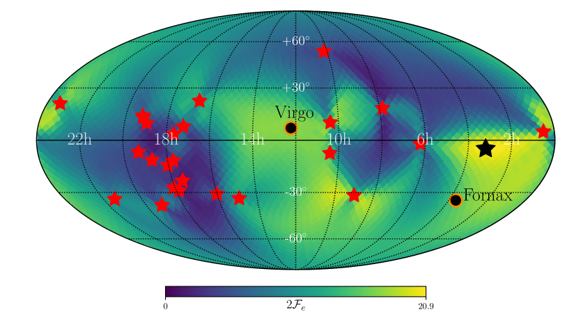
The sky distribution of $\mathcal{F}_{e}$ at this frequency is given in Figure 1. The region of high statistic value (bright yellow) is quite sparse and inconclusive with regards to the localisation of the CGW candidate. The maximum $\mathcal{F}_{e}$ is depicted by a black star and corresponds to a region of the sky where we are lacking pulsars and hence where the array is expected to be less sensitive.

The analysis was repeated by including the CURN component in the noise model and results are presented in Figure 2. We show two distributions of $\mathcal{F}_{e}$. These are both evaluated at the optimal sky position and at the GW frequency 4.64 nHz and are obtained by varying the noise parameters (random draw) with (orange histogram) and without (blue histogram) the CURN component. Inclusion of the CURN slightly reduces the significance of the CGW candidate.

To evaluate the p-value, we compute the null distribution according to the steps outlined in subsection 2.3 at the CGW candidate parameter values (maximising the noise averaged $\mathcal{F}_{e}$). These results are indicated by the grey shaded distribution in Figure 2. The theoretical $\chi^{2}$ null distribution is shown as a black curve. The scrambled distribution of $2\mathcal{F}_{e}$ is close to the theoretical $\chi^{2}_{4}$ distribution, but not completely overlapping. This could be due to (i) non-gaussian noise present in the array; (ii) the choice of the orthogonality condition ($M<0.2$) allowing the signal to leak into the distribution; or (iii) the definition of the match function which doesn’t take into account different sensitivity of pulsars in the array (Marco et al., 2023).

Refer to caption
Figure 1: $\mathcal{F}_{e}$-statistic of the candidate source at $f_{gw}=4.64$ nHz averaged over the noise uncertainties for the custom PSRN model. The black star shows the position of highest $\mathcal{F}_{e}$, whereas the red stars show the positions of the pulsars. The Fornax and Virgo clusters are shown as black dots.
Table 2: Statistical significance of the candidate source at 4.64 nHz. The p-values for the $\chi^{2}_{4}$ are obtained using the maximum likelihood noise parameters and the sky scrambled p-value from the median of the $2\mathcal{F}_{e}$ distribution. We show the p-values for the custom pulsar noise PSRN, $p(\mathcal{F}_{e})$, or also including a common uncorrelated red noise CURN+PSRN, $p(\mathcal{F}_{e,\rm{CURN}})$.
$p(\mathcal{F}_{e})$ $p(\mathcal{F}_{e,\rm{CURN}})$
$\chi^{2}_{4}$ $5\times 10^{-4}$ $1\times 10^{-3}$
Sky scrambles $(7\pm 4)\times 10^{-4}$ $(6\pm 1)\times 10^{-3}$
Refer to caption
Figure 2: Distribution of $\mathcal{F}_{e}$-statistic over the noise uncertainties without CURN (blue) and with CURN (orange) at 4.64 nHz. The null distributions of the $\mathcal{F}_{e}$ are obtained from the analysis of the EPTA DR2new data with scrambled sky positions (grey shaded region) and from the theoretical formula of a $\chi^{2}_{4}$-distribution (black solid line).

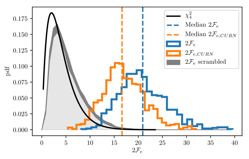
We compute p-values using the obtained null distributions and the measured median values of the orange and blue $\mathcal{F}_{e}$ distributions. The results are summarized in Table 2, the top row is for the theoretical distribution and the second row is for the scrambled null distribution (with uncertainty). The obtained p-value for $\mathcal{F}_{e}$ corresponds to about $3\sigma$ while $\mathcal{F}_{e,CURN}$ corresponds to about $2.5\sigma$.

3.2 Bayesian analysis

Refer to caption
Figure 3: Bayes factor for the model comparison PSRN+CURN+CGW (Earth term) vs PSRN+CURN for 50 logarithmically spaced frequency sub-bands in the region $f_{gw}\in[1.5,320]$ nHz.
Refer to caption
Figure 4: Posterior distributions of the CGW search in the second data release of the EPTA DR2new. The posteriors are obtained using a CGW model with Earth and pulsar term, the custom PSRN model and a CRN with either CURN or HD (GWB) correlations represented by 9 frequency bins. We show the posterior distribution for the gravitational wave frequency and amplitude $f_{gw}$, $h$ of the CGW, and the common noise spectral index and amplitude $\gamma$ and $A$. The contours indicate the 1,2,3-$\sigma$ Gaussian contours.

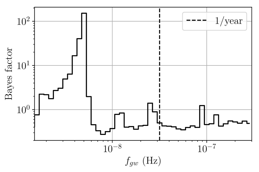
We perform a Bayesian CGW search by splitting the frequency range $10^{-9}-10^{-6.5}$ Hz into 50 logarithmically spaced subsegments and assuming Earth term only. We have computed the Bayes factor in each sub-band using PTMCMC and the product-space method. The results are presented in Figure 3 for the noise model described in Section 2. We find a Bayes factor above 100 around 4-5 nHz and we perform a detailed analysis around the small frequency range using the priors shown in Table 1.

Table 3: Bayes factors obtained for different model comparisons indicate how much the data favor the inclusion of a continuous gravitational wave (CGW) with Earth and pulsar term. The first comparison considers adding a continuous gravitational wave to the pulsar custom noise (PSRN). The second and third model comparisons include an additional common uncorrelated red noise CURN modeled with a power-law with 3 or 9 frequency bins. The fourth and fifth model comparisons include a gravitational wave background GWB modeled with a power-law with 3 or 9 frequency bins.
Model comparison Bayes factor
CGW+PSRN vs PSRN 4000
CGW+PSRN+CURN vs PSRN+CURN, 3 bins 12
CGW+PSRN+CURN vs PSRN+CURN, 9 bins 4
CGW+PSRN+GWB vs PSRN+GWB, 3 bins 1
CGW+PSRN+GWB vs PSRN+GWB, 9 bins 0.7
Refer to caption
Figure 5: Posterior distribution of the sky localization obtained by searching for a CGW in the second data release of the EPTA DR2new. The posteriors are obtained using a CGW model with Earth and pulsar term, the inclusion of the custom pulsar noise (PSRN) and a common uncorrelated red noise (CURN) represented by 9 frequency bins. For reference, we show the position of the analyzed pulsars and the Virgo and Fornax clusters.

We have compared several models describing the data using Bayes factors as the decision maker. We use Eryn (Karnesis et al., 2023) as our fiducial sampler and we crosscheck the results using PTMCMC sampler (Ellis & van Haasteren, 2017)) and QuickCW (Bécsy et al., 2022). The computation of the Bayes factors is performed using RJMCMC and confirmed with product-space method. Our findings are summarized in Table 3 and here we give a detailed description of each row. For all models with CGW described below and quoted in the table, we have assumed a circular binary described in  subsection 2.2 with Earth and pulsar term, using the priors given in Table 1 unless otherwise stated.

The simplest considered data model includes only the custom pulsar noise (PSRN), therefore, no CRN is included. The PSRN model is used as a null hypothesis, and alternative is given by the pulsar noise plus CGW (PSRN+CGW) considering Earth and pulsar terms. The Bayes factor for the model comparison PSRN+CGW vs PSRN is 4000. This indicates strong evidence for the inclusion of the CGW.

Next, we include to the custom noise PSRN a CRN: either a CURN, or a GWB correlated according to the HD pattern. These become the new null hypotheses (CURN+PSRN) and (GWB+PSRN). We also consider two descriptions for the CRN: one using the three lowest Fourier harmonics (3 bins), and one using the nine lowest Fourier harmonics (9 bins) as done in (the EPTA and InPTA Collaborations, 2023b). Since the CGW candidate is located close to the second Fourier bin, showing the results for 3 bins can help singling out the red noise components of the spectrum that might be potentially afffected by the other high frequency noises. The presence of a CGW in this model is not very prominent but definitively non-negligible. The Bayes factors of PSRN+CURN+CGW vs PSRN+CURN are 4 and 12, for 9 and 3 bins respectively. The choice of the number of bins affects the spectral properties of the CRN and, consequently, also the Bayes factors. In fact, the slope of the CURN model becomes steeper when using 3 bins, allowing the CGW, whose frequency is close to the 2nd bin, to emerge more easily than when using 9 bins. However, when including the HD correlations, the Bayes factors of PSRN+GWB+CGW vs PSRN+GWB drop to 0.7 and 1, for 9 and 3 bins, respectively.

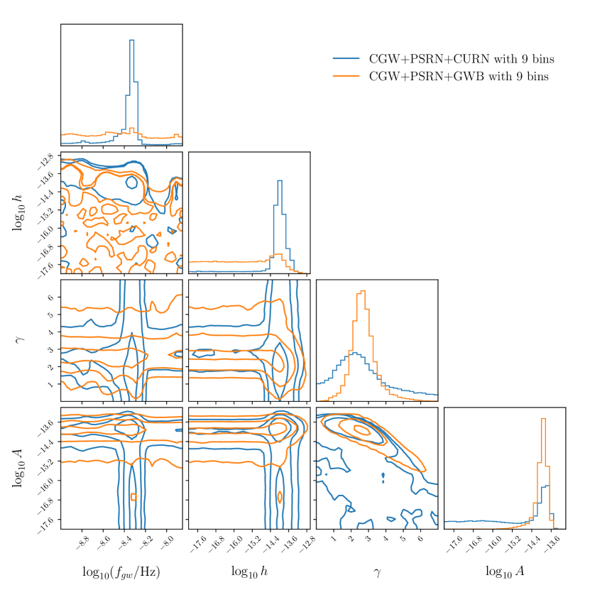
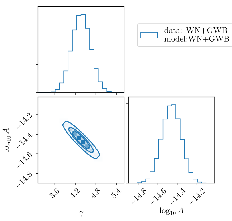
As already was pointed out in (the EPTA and InPTA Collaborations, 2023b), the HD component of the noise absorbs most of CGW signal and this can be clearly seen in the drop of the Bayes factor and in the posterior distributions shown in Figure 4. When the CRN is a CURN, the CGW model absorbs the power of the background around $\log_{10}f_{gw}\in[-8.5,-8.2]$ and yields an amplitude $\log_{10}A$ posterior distribution with tails extending up to the lowest end of the prior range (see correlation in Figure 4 for parameters $\log_{10}f_{gw},\log_{10}A$).

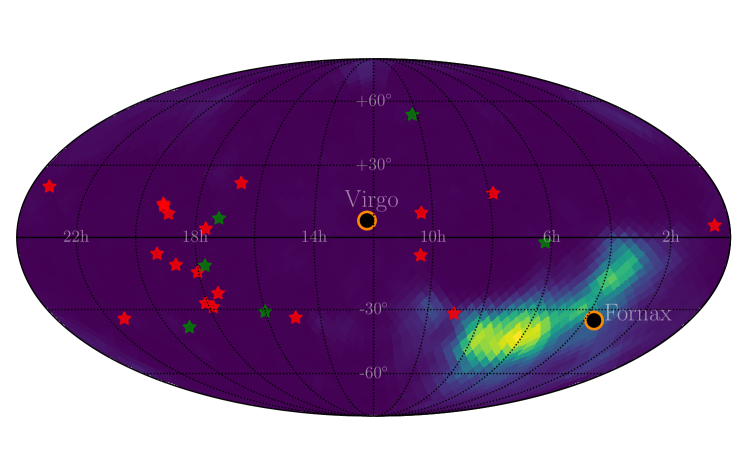
For the model CURN+PSRN+CGW with 9 bins, the log-frequency $f_{gw}$ is measured to be $4.61^{+1.11}_{-2.98}$ nHz and the log-amplitude $\log_{10}h$ is measured to be $-14.0^{+0.5}_{-2.6}$ (median and symmetric 90% credible interval). The chirp-mass posterior is uninformative and the sky localization posterior is shown in Figure 5 where we also show the Virgo and Fornax clusters which are $16.5$ Mpc and $19.3$ Mpc from the Earth Jordan et al. (2007), respectively. If we use the median values of the amplitude and frequency to estimate the luminosity distance, we obtain $d_{L}\approx 16.6\,({\mathcal{M}}/{10^{9}{\rm M}_{\odot}})^{5/3}\,{\rm Mpc},$ using Equation 5.

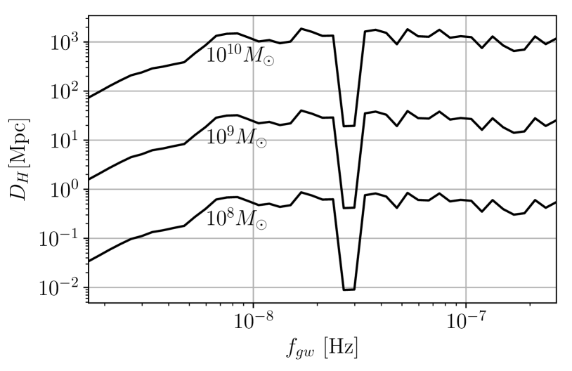
We compute the sky marginalized 95% upper limit on strain amplitude, $h_{95}(f_{gw})$, across the studied frequency range for the model PSRN+CURN+CGW with 9 bins. For this analysis, we used a uniform prior on $h$ in the range $[10^{-18},10^{-11}]$ instead of the uniform prior on $\log_{10}h$ used for the search (see Arzoumanian et al. (2023); Falxa et al. (2023)). The strain upper limit was converted into a horizon distance, $D_{H}$, (i.e., the distance up to which SMBHB systems should produce detectable CGW signals) using Equation 5:

$$D_{H}=2\frac{\mathcal{M}^{5/3}}{h_{95}}(\pi f_{gw})^{2/3}.$$ (10)

We plot $D_{H}$ as a function of $f_{gw}$ in Figure 6 for three values of chirp mass $\mathcal{M}=[10^{8}M_{\odot},10^{9}M_{\odot},10^{10}M_{\odot}]$. The highest $D_{H}$ is recovered around 20 nHz. The closest galaxy-cluster candidates (Fornax and Virgo) that could host a SMBHB lie at distances larger than 10 Mpc, meaning that we need binary systems with chirp masses larger than $10^{9}M_{\odot}$ in order for them to be detectable.

Refer to caption
Figure 6: Horizon luminosity distance, $D_{H}$, obtained from the sky averaged 95% upper limit on strain amplitude $h$ using the PSRN+CURN+CGW (Earth term + pulsar term) model. The horizon distance is calculated with Equation 10 for three chirp masses: $10^{8}M_{\odot}$, $10^{9}M_{\odot}$ and $10^{10}M_{\odot}$.
Refer to caption
Figure 7: Inference of the amplitude $h$ and frequency $f_{gw}$ of CGW using the PSRN+CURN+CGW model. The results obtained with Eryn are shown as green and blue histograms, for a Earth term only, and full CGW model, respectively. The blue contours are to be compared with the orange posterior obtained with QuickCW. The shown contours are the 90% normal credible regions.

We have also used this model (CURN+PSRN+CGW) to investigate the effect of the pulsar term and to cross-check the samplers. The narrow green posterior contours in Figure 7 correspond to using Eryn to sample the model with the Earth-term only and the broad blue posterior is inferred with the model including the pulsar term. We have overplotted in orange similar results (including the pulsar term) obtained with the QuickCW sampler. To check if the circular CGW model is appropriate, we carried out a separate analysis including orbital eccentricity in the model following Taylor et al. (2016), but using only Earth term in the analysis. This analysis inferred a low eccentricity ($e<0.2$) for the CGW candidate, indicating that the analysis performed with the circular binary model is adequate.

Refer to caption
Figure 8: Posterior distributions of the CGW search in the second data release of the EPTA DR2new. The posteriors are obtained using a CGW model with Earth and pulsar term, the custom PSRN model and an HD correlated background (GWB) represented by 9 and 3 frequency bins. We show the posterior distribution for the gravitational wave frequency and amplitude $f_{gw},h$ of the CGW, and the common noise spectral index and amplitude $\gamma$ and $A$. The contours indicate the 1,2,3-$\sigma$ Gaussian contours.

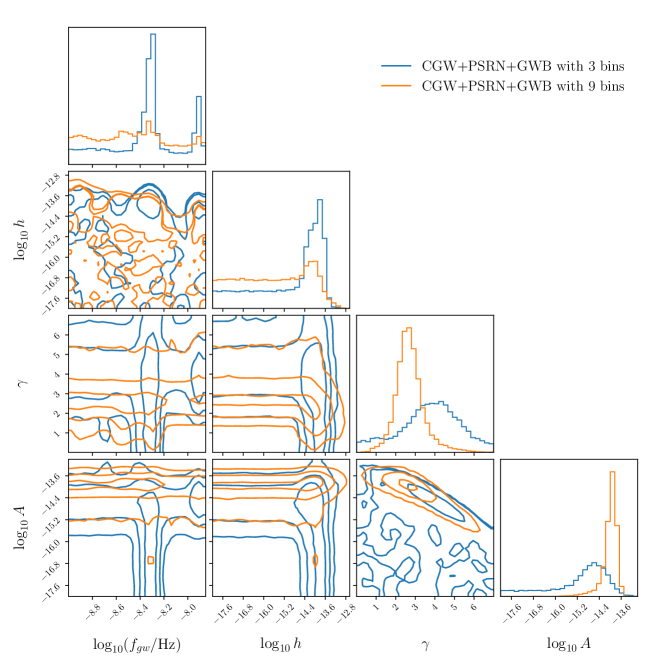
For the model GWB+PSRN+CGW with 9 bins, we cannot constrain the CGW parameters, so we set a 95% upper limit on $\log_{10}h_{95\%}=-13.75$. We constrain the spectral properties of the GWB background to be $2.66_{-1.02}^{+1.43}$ and $-13.95_{-0.62}^{+0.25}$, respectively for $\gamma$ and $\log_{10}A)$ (median and symmetric 90% credible interval). The picture changes if we use a different number of frequency bins. We show in Figure 8 the posteriors for the same model GWB+PSRN+CGW, but this time with 9 and 3 bins. It is clear that the spectral properties ($\gamma$ and $A$) of the background are affected by the number of bins. The median log-amplitude decreases from -13.95 to -14.34 and the median slope from 2.66 to 3.832, following the typical $\gamma-\log_{10}A$ correlation. The steeper slope allows the CGW to emerge from the noise and its posteriors show two clear peaks, one at 4.64 nHz and one at 12.6 nHz.

3.3 Optimal Statistics

The Bayesian analysis presented in the previous subsection indicates that the results are inconclusive about the nature of the observed signal. This subsection starts a long investigation process attempting to answer the question: “what is it that we see?” and provides a transition to the next section which describes analysis of the simulated data.

We compute the signal-to-noise ratio (SNR) of the CRN using the optimal statistic approach (Chamberlin et al., 2015; Vigeland et al., 2018) implemented within enterprise_extensions software package (Taylor et al., 2021). We estimate the SNR assuming quadrupolar correlation (HD). Following the procedure outlined in (the EPTA and InPTA Collaborations, 2023b; Vigeland et al., 2018), we vary the noise parameters (using the results of (the EPTA and InPTA Collaborations, 2023a)) and get as a result a distribution of SNR. The solid orange line in Figure 9 reproduces the findings reported in (the EPTA and InPTA Collaborations, 2023b).

Next we include CGW in the model: we use the posterior samples obtained in the Bayesian analysis which preserve the correlation between the noise parameters and CGW (instead of only the noise parameters), and re-evaluate the optimal statistic. The resulting SNR distribution of HD correlations is given in Figure 9 as dashed orange line. This result implies that the data (minus CGW) does not show any sign of quadrupolar (GWB) correlation, in other words, a CGW alone can explain the HD feature observed in the data.

We corroborate our results obtained on the EPTA DR2new by repeating the same analysis on a simulated dataset. We produce a fake PTA based on the real (EPTA DR2new) pulsars and the noise estimation in which we inject only one CGW and no GWB (see Section 4 for a detailed description of the simulation). The blue solid line in Figure 9 indeed resembles the result obtained on the DR2new (orange line). As we will discuss in details in the next section, a single CGW signal could be interpreted as GWB (see Allen (2023)). The subtraction of the CGW from the timing residuals, as expected, removes the quadrupolar correlation (blue dashed line) and well reproduces the previously obtained results on the EPTA data.

Refer to caption
Figure 9: Distributions of the signal-to-noise-ratio (SNR) for the HD correlations for a common red process with $\gamma=13/3$, with (dashed) or without (solid) adding CGW to the data model. The orange lines correspond to the results obtained on DR2new and blue are on the simulated data with only CGW (no CRN).

4 Simulation

We perform a simulation campaign to try to reproduce the features observed in the analysis of DR2new. We generate a fake array with the same time of arrivals (TOA)s and pulsar positions as in the real dataset. We inject noises using the maximum a posteriori of the noise parameter posterior obtained in the EPTA and InPTA Collaborations (2023a). We use a Gaussian process to simulate the noise components and consider different realizations in order to reproduce the observed results (see Appendix A). Using the simulated array as a basis, we propose two cases to study:

  • PSRN+CGW: A simulated analogue of DR2new with only one circular CGW injected at 4.8 nHz with sky location at (3h38, -3527) as if it was in the Fornax cluster with a chirp mass of $10^{9.2}M_{\odot}$ and amplitude $h=10^{-13.6}$, without any CRN.

  • PSRN+GWB: A simulated analogue of DR2new with a gaussian and isotropic GWB as CRN with a powerlaw spectrum corresponding to $A=10^{-14.5}$ and spectral index $\gamma=13/3$ (without any CGW).

Each simulation is analysed with the custom PSRN model and either with CGW (using the Earth term only) or GWB with a powerlaw spectrum.

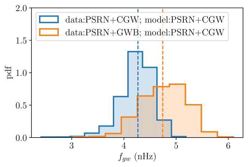
We have considered the PSRN+GWB simulated data and analysed it with a single CGW source (no GWB). In Figure 10 we show that we can recover the CGW even if we have injected an isotropic GWB. We have repeated the analysis on 10 simulated datasets, in most cases the recovered “CGW” was centered at the lowest Fourier bin ($1/T_{obs}\sim 3$ nHz) and located in the close vicinity of pulsars, in many cases around J1713+0747.

However, in 2 GWB injections out of 10, we recover a CGW frequency around 4-5 nHz (similar to what we observe in DR2new) with a Bayes factor PSRN+CGW over PSRN only of about 5000. We present the posterior frequency of that particular case as a orange histogram in Figure 10. We have also analysed this data using GWB model and the inferred posterior is given in orange in Figure 11.

Next we consider the PSRN+CGW simulated data and analyse it with the model of isotropic GWB with a power-law spectrum. As expected, this model gives a very constrained posteriors and high Bayes factor of 2600. Indeed, the excess of power at low frequency gives support to a power-law spectrum (though not the best description) and HD correlations are reproduced by averaging over the pulsar pairs (see Allen (2023); Cornish & Sesana (2013) for details). The analysis of this dataset with a CGW model is shown in Figure 10 as a blue histogram. Analysis of the same data with GWB is given in Figure 11 as a blue posterior. One can see that posterior has a lower amplitude and is shallower.

It is important to note that the recovered GWB parameters on Figure 11 are different from their injected values for the PSRN+GWB simulation. This is due to strong correlations between the signal and the individual pulsar red noise models. We made a simulation where only white noise is injected (contrary to the realistic simulation where we inject the full PSRN noise model) with a GWB and no CGW, revealing that in that case we correctly recover the injected values of signal parameters (see Figure 12).

The analysis of the simulated data confirms that it is hard to reliably identify the nature of the CRN: whether it is a CGW or a GWB. The point source also produces HD correlations, as previously shown in (Cornish & Sesana, 2013; Bécsy et al., 2022; Allen, 2023). Moreover, the anisotropic configuration of the current PTA (pulsars not uniformly distributed in the sky and having very different noise properties) produces an uneven response across the sky and the studied frequency range. The resulting discrepancies between the injected and recovered parameter values due to the interactions between the PSRN and signal models are still not fully understood and need to be investigated more thoroughly in future analyses. We need to invent further consistency checks (like anisotropy, for example) or wait for longer datasets. Hopefully the inclusion of pulsars from the southern hemisphere (PPTA) could help us to break this parity.

Refer to caption
Figure 10: Posterior distribution of the gravitational wave frequency $f_{gw}$ of a CGW fitted to two simulated PTAs: one with a single injected CGW (PSRN+CGW blue histogram), and one with an injected GWB (PSRN+GWB orange histogram). The posterior distribution is obtained with a MCMC analysis for a PSRN+CGW (Earth term) model. The dashed lines are the medians of the distributions.
Refer to caption
Figure 11: Posterior distribution of amplitude $\log_{10}A$ and spectral index $\gamma$ of the GWB for two simulated PTAs : 1 realistic PTA with only 1 CGW injected (PSRN+CGW) and 1 realistic PTA with a GWB injected (PSRN+GWB). The posterior distribution is obtained with a MCMC analysis for a PSRN+GWB model. The recovered GWB parameters are different from the injected ones for the PSRN+GWB simulation due to strong correlations between the injected PSRN and GWB models.
Refer to caption
Figure 12: Posterior distribution of amplitude $\log_{10}A$ and spectral index $\gamma$ of the GWB for a simulated PTA with only white noise (WN) and an injected GWB with a powerlaw spectrum corresponding to $A=10^{-14.5}$ and spectral index $\gamma=13/3$. We see that the recovered values correctly match the injected ones when only white noise is added to the array.

5 Summary

This paper presents an analysis of the EPTA DR2new dataset searching for continuous GW signals from super-massive black hole binaries in quasi-circular orbits. We perform a frequentist (based on $\mathcal{F}_{e}$-statistic) and Bayesian (using Bayes factor) analysis of the data, and, in both cases, find a significant CGW candidate at 4-5.6 nHz. The frequentist analysis gives a p-value of ($5\times 10^{-4}$ $6\times 10^{-3}$), equivalent to a 2.5-3$\sigma$ significance level, depending on the evaluation procedure and whether or not a CURN is included in the noise model. Within the Bayesian analysis of the CGW candidate, we computed the Bayes factor between models containing CGW and noise-only. We see strong evidence (Bayes factor $\sim 4000$) of CGW if we consider only PSRN (individual pulsar noise) in the alternative hypothesis, weak evidence (Bayes factors $\sim 4-12$) if we include a CURN process in the alternative hypothesis, and completely inconclusive if the CRN is assumed to have the correlation of a GWB (Bayes factors $\sim 0.7-1$). In other words, the data is equally well described by a model including both a GWB and CGW and a model including GWB only. We note that the CGW model depends on 58 parameters and therefore comes with a large dimensionality penalty. Despite this, the Bayes factor is close to unity. In addition, we have shown that removing the CGW candidate from the data destroys HD correlations, as seen from the computation of the optimal statistic.

In an attempt to understand if the observed signal is due to a GWB or a CGW, we perform a simulation campaign. We simulate data based on the noise parameters inferred in the EPTA and InPTA Collaborations (2023a) and inject a GW signal. Our main finding is that simulated data with only an isotropic GWB injected can be fitted with a CGW model, and vice versa; a GWB model can explain simulated data containing only a single injected CGW. Therefore, we cannot conclusively distinguish between the presence of a single continuous gravitational wave or a gravitational wave background. In the EPTA and InPTA Collaborations (2023c), considering models that produce a GW signal consistent with the one present in DR2new, the probability of detecting a single source with SNR larger than 3 is estimated to be 50%.

We hope that an analysis of the combined IPTA data (Data Release 3) will help to confirm the presence or not of a CGW signal and shed light on its nature.

Acknowledgements.
The European Pulsar Timing Array (EPTA) is a collaboration between European and partner institutes, namely ASTRON (NL), INAF/Osservatorio di Cagliari (IT), Max-Planck-Institut für Radioastronomie (GER), Nançay/Paris Observatory (FRA), the University of Manchester (UK), the University of Birmingham (UK), the University of East Anglia (UK), the University of Bielefeld (GER), the University of Paris (FRA), the University of Milan-Bicocca (IT), the Foundation for Research and Technology, Hellas (GR), and Peking University (CHN), with the aim to provide high-precision pulsar timing to work towards the direct detection of low-frequency gravitational waves. An Advanced Grant of the European Research Council allowed to implement the Large European Array for Pulsars (LEAP) under Grant Agreement Number 227947 (PI M. Kramer). The EPTA is part of the International Pulsar Timing Array (IPTA); we thank our IPTA colleagues for their support and help with this paper and the external Detection Committee members for their work on the Detection Checklist. Part of this work is based on observations with the 100-m telescope of the Max-Planck-Institut für Radioastronomie (MPIfR) at Effelsberg in Germany. Pulsar research at the Jodrell Bank Centre for Astrophysics and the observations using the Lovell Telescope are supported by a Consolidated Grant (ST/T000414/1) from the UK’s Science and Technology Facilities Council (STFC). ICN is also supported by the STFC doctoral training grant ST/T506291/1. The Nançay radio Observatory is operated by the Paris Observatory, associated with the French Centre National de la Recherche Scientifique (CNRS), and partially supported by the Region Centre in France. We acknowledge financial support from “Programme National de Cosmologie and Galaxies” (PNCG), and “Programme National Hautes Energies” (PNHE) funded by CNRS/INSU-IN2P3-INP, CEA and CNES, France. We acknowledge financial support from Agence Nationale de la Recherche (ANR-18-CE31-0015), France. The Westerbork Synthesis Radio Telescope is operated by the Netherlands Institute for Radio Astronomy (ASTRON) with support from the Netherlands Foundation for Scientific Research (NWO). The Sardinia Radio Telescope (SRT) is funded by the Department of University and Research (MIUR), the Italian Space Agency (ASI), and the Autonomous Region of Sardinia (RAS) and is operated as a National Facility by the National Institute for Astrophysics (INAF). The work is supported by the National SKA programme of China (2020SKA0120100), Max-Planck Partner Group, NSFC 11690024, CAS Cultivation Project for FAST Scientific. This work is also supported as part of the “LEGACY” MPG-CAS collaboration on low-frequency gravitational wave astronomy. JA acknowledges support from the European Commission (Grant Agreement number: 101094354). JA and SCha were partially supported by the Stavros Niarchos Foundation (SNF) and the Hellenic Foundation for Research and Innovation (H.F.R.I.) under the 2nd Call of the “Science and Society – Action Always strive for excellence – Theodoros Papazoglou” (Project Number: 01431). AC acknowledges support from the Paris Île-de-France Region. AC, AF, ASe, ASa, EB, DI, GMS, MBo acknowledge financial support provided under the European Union’s H2020 ERC Consolidator Grant “Binary Massive Black Hole Astrophysics” (B Massive, Grant Agreement: 818691). GD, KLi, RK and MK acknowledge support from European Research Council (ERC) Synergy Grant “BlackHoleCam”, Grant Agreement Number 610058. This work is supported by the ERC Advanced Grant “LEAP”, Grant Agreement Number 227947 (PI M. Kramer). AV and PRB are supported by the UK’s Science and Technology Facilities Council (STFC; grant ST/W000946/1). AV also acknowledges the support of the Royal Society and Wolfson Foundation. JPWV acknowledges support by the Deutsche Forschungsgemeinschaft (DFG) through thew Heisenberg programme (Project No. 433075039) and by the NSF through AccelNet award #2114721. NKP is funded by the Deutsche Forschungsgemeinschaft (DFG, German Research Foundation) – Projektnummer PO 2758/1–1, through the Walter–Benjamin programme. ASa thanks the Alexander von Humboldt foundation in Germany for a Humboldt fellowship for postdoctoral researchers. APo, DP and MBu acknowledge support from the research grant “iPeska” (P.I. Andrea Possenti) funded under the INAF national call Prin-SKA/CTA approved with the Presidential Decree 70/2016 (Italy). RNC acknowledges financial support from the Special Account for Research Funds of the Hellenic Open University (ELKE-HOU) under the research programme “GRAVPUL” (grant agreement 319/10-10-2022). EvdW, CGB and GHJ acknowledge support from the Dutch National Science Agenda, NWA Startimpuls – 400.17.608. BG is supported by the Italian Ministry of Education, University and Research within the PRIN 2017 Research Program Framework, n. 2017SYRTCN. LS acknowledges the use of the HPC system Cobra at the Max Planck Computing and Data Facility. The Indian Pulsar Timing Array (InPTA) is an Indo-Japanese collaboration that routinely employs TIFR’s upgraded Giant Metrewave Radio Telescope for monitoring a set of IPTA pulsars. BCJ, YG, YM, SD, AG and PR acknowledge the support of the Department of Atomic Energy, Government of India, under Project Identification # RTI 4002. BCJ, YG and YM acknowledge support of the Department of Atomic Energy, Government of India, under project No. 12-R&D-TFR-5.02-0700 while SD, AG and PR acknowledge support of the Department of Atomic Energy, Government of India, under project no. 12-R&D-TFR-5.02-0200. KT is partially supported by JSPS KAKENHI Grant Numbers 20H00180, 21H01130, and 21H04467, Bilateral Joint Research Projects of JSPS, and the ISM Cooperative Research Program (2021-ISMCRP-2017). AS is supported by the NANOGrav NSF Physics Frontiers Center (awards #1430284 and 2020265). AKP is supported by CSIR fellowship Grant number 09/0079(15784)/2022-EMR-I. SH is supported by JSPS KAKENHI Grant Number 20J20509. KN is supported by the Birla Institute of Technology & Science Institute fellowship. AmS is supported by CSIR fellowship Grant number 09/1001(12656)/2021-EMR-I and T-641 (DST-ICPS). TK is partially supported by the JSPS Overseas Challenge Program for Young Researchers. We acknowledge the National Supercomputing Mission (NSM) for providing computing resources of ‘PARAM Ganga’ at the Indian Institute of Technology Roorkee as well as ‘PARAM Seva’ at IIT Hyderabad, which is implemented by C-DAC and supported by the Ministry of Electronics and Information Technology (MeitY) and Department of Science and Technology (DST), Government of India. DD acknowledges the support from the Department of Atomic Energy, Government of India through Apex Project - Advance Research and Education in Mathematical Sciences at IMSc. The work presented here is a culmination of many years of data analysis as well as software and instrument development. In particular, we thank Drs. N. D’Amico, P. C. C. Freire, R. van Haasteren, C. Jordan, K. Lazaridis, P. Lazarus, L. Lentati, O. Löhmer and R. Smits for their past contributions. We also thank Dr. N. Wex for supporting the calculations of the galactic acceleration as well as the related discussions. The EPTA is also grateful to staff at its observatories and telescopes who have made the continued observations possible. Author contributions. The EPTA is a multi-decade effort and all authors have contributed through conceptualisation, funding acquisition, data-curation, methodology, software and hardware developments as well as (aspects of) the continued running of the observational campaigns, which includes writing and proofreading observing proposals, evaluating observations and observing systems, mentoring students, developing science cases. All authors also helped in (aspects of) verification of the data, analysis and results as well as in finalising the paper draft. Specific contributions from individual EPTA members are listed in the CRediT444https://credit.niso.org/ format below. InPTA members contributed in uGMRT observations and data reduction to create the InPTA data set which is employed while assembling the DR2full+ and DR2new+ data sets.

References

  • Allen (2023) Allen, B. 2023, Physical Review D, 107
  • Arzoumanian et al. (2023) Arzoumanian, Z., Baker, P. T., Blecha, L., et al. 2023, The NANOGrav 12.5-year Data Set: Bayesian Limits on Gravitational Waves from Individual Supermassive Black Hole Binaries
  • Babak & Sesana (2012) Babak, S. & Sesana, A. 2012, Phys. Rev. D, 85, 044034
  • Bécsy et al. (2022) Bécsy, B., Cornish, N. J., & Digman, M. C. 2022, Phys. Rev. D, 105, 122003
  • Bécsy et al. (2022) Bécsy, B., Cornish, N. J., & Kelley, L. Z. 2022, The Astrophysical Journal, 941, 119
  • Chalumeau et al. (2022) Chalumeau, A., Babak, S., Petiteau, A., et al. 2022, MNRAS, 509, 5538
  • Chamberlin et al. (2015) Chamberlin, S. J., Creighton, J. D. E., Siemens, X., et al. 2015, Phys. Rev. D, 91, 044048
  • Chen et al. (2021) Chen, S., Caballero, R. N., Guo, Y. J., et al. 2021, MNRAS, 508, 4970
  • Corbin & Cornish (2010) Corbin, V. & Cornish, N. J. 2010, Pulsar Timing Array Observations of Massive Black Hole Binaries
  • Cornish & Sesana (2013) Cornish, N. J. & Sesana, A. 2013, Classical and Quantum Gravity, 30, 224005
  • Ellis & van Haasteren (2017) Ellis, J. & van Haasteren, R. 2017, jellis18/PTMCMCSampler: Official Release
  • Ellis et al. (2012) Ellis, J. A., Siemens, X., & Creighton, J. D. E. 2012, Astrophys. J., 756, 175
  • Ellis et al. (2020) Ellis, J. A., Vallisneri, M., Taylor, S. R., & Baker, P. T. 2020, ENTERPRISE: Enhanced Numerical Toolbox Enabling a Robust PulsaR Inference SuitE, Zenodo
  • Falxa et al. (2023) Falxa, M., Babak, S., Baker, P. T., et al. 2023, Monthly Notices of the Royal Astronomical Society, 521, 5077
  • Górski et al. (2005) Górski, K. M., Hivon, E., Banday, A. J., et al. 2005, ApJ, 622, 759
  • Hee et al. (2016) Hee, S., Handley, W. J., Hobson, M. P., & Lasenby, A. N. 2016, MNRAS, 455, 2461
  • Jordan et al. (2007) Jordan, A., Blakeslee, J. P., Cote, P., et al. 2007, Astrophys. J. Suppl., 169, 213
  • Karnesis et al. (2023) Karnesis, N., Katz, M. L., Korsakova, N., Gair, J. R., & Stergioulas, N. 2023 [arXiv:2303.02164]
  • Marco et al. (2023) Marco, V. D., Zic, A., Miles, M. T., et al. 2023, Toward robust detections of nanohertz gravitational waves
  • Skilling (2004) Skilling, J. 2004, in American Institute of Physics Conference Series, Vol. 735, Bayesian inference and maximum entropy methods in science and engineering, ed. R. Fischer, R. Preuss, & U. von Toussaint, 395–405
  • Speri et al. (2023) Speri, L., Porayko, N. K., Falxa, M., et al. 2023, MNRAS, 518, 1802
  • Taylor et al. (2021) Taylor, S. R., Baker, P. T., Hazboun, J. S., Simon, J., & Vigeland, S. J. 2021, enterprise_extensions
  • Taylor et al. (2016) Taylor, S. R., Huerta, E. A., Gair, J. R., & McWilliams, S. T. 2016, Astrophys. J., 817, 70
  • Taylor et al. (2017) Taylor, S. R., Lentati, L., Babak, S., et al. 2017, Phys. Rev. D, 95, 042002
  • the EPTA and InPTA Collaborations (2023a) the EPTA and InPTA Collaborations. 2023a, å, this Volume
  • the EPTA and InPTA Collaborations (2023b) the EPTA and InPTA Collaborations. 2023b, å, this Volume
  • the EPTA and InPTA Collaborations (2023c) the EPTA and InPTA Collaborations. 2023c, å, this Volume
  • van Haasteren & Vallisneri (2014) van Haasteren, R. & Vallisneri, M. 2014, Phys. Rev. D, 90, 104012
  • Verbiest et al. (2012) Verbiest, J. P. W., Weisberg, J. M., Chael, A. A., Lee, K. J., & Lorimer, D. R. 2012, The Astrophysical Journal, 755, 39
  • Vigeland et al. (2018) Vigeland, S. J., Islo, K., Taylor, S. R., & Ellis, J. A. 2018, Phys. Rev. D, 98, 044003
  • Zonca et al. (2019) Zonca, A., Singer, L., Lenz, D., et al. 2019, Journal of Open Source Software, 4, 1298

Appendix A Simulation

The simulations were performed using the fakepta package (https://github.com/mfalxa/fakepta). The injected noises are assumed to be stationary gaussian processes with a power spectral density $S_{n}(f,{\alpha})$ function of frequency $f$ and hyper-parameters ${\alpha}$ according to the EPTA and InPTA Collaborations (2023a). In time domain, such noises $n({t})$ can be decomposed on a Fourier basis of size $N$:

$$n({t})=\sum_{k=1}^{N}X_{k}\sin(2\pi k{t}/T_{obs})+Y_{k}\cos(2\pi k{t}/T_{obs})=\textbf{F}{a},$$ (11)

where we rewrote the sum as a matrix-vector multiplication with ${a}$ a vector of $(X_{k},Y_{k})$ and F the design matrix of size $N_{\rm TOAs}\times N$ containing the sine and cosine terms $\sin(2\pi k{t}/T_{obs}),\cos(2\pi k{t}/T_{obs})$ per each TOA.

The covariance matrix $\textbf{C}_{n}({t},{t^{\prime}})$ of the gaussian process $n(t)$ is given by the expectation value $\langle\rangle$ of the noise at two times:

$$\textbf{C}_{n}({t},{t^{\prime}})=\langle n({t}),n({t^{\prime}})\rangle=\textbf{F}^{\intercal}\langle{a}^{2}\rangle\textbf{F}=\textbf{F}^{\intercal}{\Phi}\textbf{F}$$ (12)

with ${\Phi}=\textrm{diag}\big{\{}S_{n}(k/T_{obs})/T_{obs}\big{\}}$.

Considering that the stochastic process $n({t})$ follows a multivariate gaussian distributions $\mathcal{N}({0},\textbf{C}_{n})$, a random realisation of $n({t})$ corresponds to a random draw from the distribution $\mathcal{N}({0},\textbf{C}_{n})$. The noises are injected by summing the obtained $n({t})$ to the simulated pulsar residuals for the maximum a posteriori set of noise hyper-parameters ${\alpha}$ (entering in the $S_{n}$) inferred from the real data.