The NANOGrav 15-year Data Set: Observations and Timing of 68 Millisecond Pulsars

Abstract

We present observations and timing analyses of 68 millisecond pulsars (MSPs) comprising the 15-year data set of the North American Nanohertz Observatory for Gravitational Waves (NANOGrav). NANOGrav is a pulsar timing array (PTA) experiment that is sensitive to low-frequency gravitational waves. This is NANOGrav’s fifth public data release, including both “narrowband” and “wideband” time-of-arrival (TOA) measurements and corresponding pulsar timing models. We have added 21 MSPs and extended our timing baselines by three years, now spanning nearly 16 years for some of our sources. The data were collected using the Arecibo Observatory, the Green Bank Telescope, and the Very Large Array between frequencies of 327 MHz and 3 GHz, with most sources observed approximately monthly. A number of notable methodological and procedural changes were made compared to our previous data sets. These improve the overall quality of the TOA data set and are part of the transition to new pulsar timing and PTA analysis software packages. For the first time, our data products are accompanied by a full suite of software to reproduce data reduction, analysis, and results. Our timing models include a variety of newly detected astrometric and binary pulsar parameters, including several significant improvements to pulsar mass constraints. We find that the time series of 23 pulsars contain detectable levels of red noise, 10 of which are new measurements. In this data set, we find evidence for a stochastic gravitational-wave background.

1 Introduction

Pulsar timing arrays (PTAs) use high-precision timing of pulsars to attempt to directly detect and study nHz-frequency gravitational waves (GWs). The idea was first proposed in the 1970s (Sazhin, 1978; Detweiler, 1979), but it was not until the discovery of millisecond pulsars (MSPs; Backer et al., 1982; Alpar et al., 1982), and the possibility of long-term microsecond-level timing with many MSPs that the idea became practical (e.g., Foster & Backer, 1990). For recent reviews on the technique and the science that can result, see Hobbs & Dai (2017); Tiburzi (2018); Taylor (2021); Verbiest et al. (2021).

PTA data are meticulously acquired for dozens of MSPs on cadences of days to months using the world’s largest radio telescopes. Sophisticated digital hardware synchronously averages the faint pulsar signals at multiple radio frequencies from a few hundred MHz to several GHz. After calculation of times of arrival (TOAs), PTAs regularly analyze these data and release them to the public.

The North American Nanohertz Observatory for Gravitational Waves (NANOGrav; Ransom et al., 2019) was formed in 2007 and has previously published four data releases (see below). Other PTA collaborations include the European PTA (EPTA; Chen et al., 2021), the Parkes PTA (PPTA; Reardon et al., 2021), and the Indian PTA (InPTA; Tarafdar et al., 2022). All four collaborations comprise the International PTA (IPTA) and earlier versions of NANOGrav, EPTA, and PPTA data sets have been combined into IPTA data releases known as IPTA DR1 (Hobbs et al., 2010) and IPTA DR2 (Perera et al., 2019). The IPTA continues to grow, and soon the InPTA and MeerKAT PTA project will begin to contribute data to IPTA data sets (Tarafdar et al., 2022; Miles et al., 2023).

This paper describes the latest release of NANOGrav data, the “15-year Data Set,” which we have collected over more than 15 years using the Arecibo Observatory, the Green Bank Telescope (GBT), and the Very Large Array (VLA). The data and analysis procedures we describe are based on and extend those from our earlier releases, which are known as our 5-year (Demorest et al., 2013, herein NG5), 9-year (Arzoumanian et al., 2015, herein NG9), 11-year (Arzoumanian et al., 2018, herein NG11), and 12.5-year “narrowband” (Alam et al., 2021a, herein NG12) and 12.5-year “wideband” data sets (Alam et al., 2021b, herein NG12WB). We will similarly refer to the present 15-year data set as NG15.

The data release reported on in this paper is an improvement upon previous NG12 and NG12WB data sets in several ways. It includes 21 additional MSPs (for a total of 68 MSPs) and an additional $\sim$2.9 years of timing baseline for the 47 continuing MSPs. We have used a new Python-based timing pipeline, utilizing Jupyter notebooks, that relies on PINT as the primary timing software (Luo et al., 2021). We are concurrently releasing both the traditional “narrowband” TOAs derived from many subbands of our radio observing bands, and “wideband” TOAs derived using the methodology of Pennucci et al. (2014) and Pennucci (2019). We have added VLA data on six pulsars, one of which is a new addition to the PTA, and have included all of the Arecibo data available up until we were no longer able to use the telescope in 2020 August, four months before its tragic collapse in 2020 December. The data included in this release will also be included in the third data release (DR3) of the IPTA.

This work is presented alongside a GW analysis searching for a GWB in the 15-yr data set (Agazie et al., 2023b, hereafter NG15gwb), detailed noise analysis of our PTA detector (Agazie et al., 2023c, NG15detchar), and astrophysical interpretation of the GWB results (Agazie et al., 2023a; Afzal et al., 2023). NANOGrav’s most recent GW results for the NG12 data set can be found in Arzoumanian et al. (2020) for the stochastic gravitational wave background (GWB), Arzoumanian et al. (2021a) for non-Einsteinian polarization modes in the GWB, Arzoumanian et al. (2021b) for constraints on cosmological phase transitions, and Arzoumanian et al. (2023) for GWs from continuous wave sources.

The plan for this paper is as follows. In Sections 2 and 3, we describe the observations and data reduction, respectively. In Section 4, we describe timing models fit to the TOAs for each pulsar, including both deterministic astrophysical phenomena and stochastic noise terms. In Section 5, we compare timing models from this data set with those from NG12 and report on any newly-significant astrometric, binary, and noise parameters. In Section 6, we acknowledge pulsar surveys that have discovered new MSPs included in this data set and we present flux density measurements for these new pulsars at two or more radio frequencies. In Section 7, we summarize the work.

The NANOGrav 15-year data set files include narrowband and wideband TOAs developed in the present paper, parameterized timing models for all pulsars for each of the TOA sets, configuration files used to run our timing analysis notebooks, and support files such as telescope clock offset measurements. The data set presented here is preserved on Zenodo at doi:10.5281/zenodo.7967585. Raw telescope data products are also available from the same website, as is code used to do all of the analysis described here. A living repository of PINT-based timing analysis software born out of this work can be found at https://github.com/nanograv/pint_pal.

2 Observations

The NANOGrav 15-year data set contains data from the 100-m GBT, the 305-m telescope at the Arecibo Observatory (Arecibo) prior to its cable failure and eventual collapse, and the 27 25-m antennae of the VLA. The procedures we used are nearly identical to those in NG9, NG11, and NG12. As in NG12, we have generated and analyzed both narrowband and wideband TOAs; we present both narrowband (NB) and wideband (WB) versions of the data set in this work. While the fundamental data reduction and timing procedures have not changed significantly from our previous releases, for this data set substantial effort was put into software development, with a major goal of improving versioning and reproducibility of results. Our new timing pipeline streamlines the iterative nature of our analyses and allows documentation of changes made to the software version, TOAs, timing solution, or noise model. The pipeline will be discussed further in Section 4. Here we describe the observations and data reduction used to generate the TOAs in this data set.

2.1 Data Collection

The present data set contains timing data and solutions for 68 MSPs, 21 more than were included in NG12. A summary of the pulsars and their timing baselines for this data set is given in Figure 1. This large increase in the number of MSPs in this data set results from two factors: first, NANOGrav tested the suitability of many newly discovered MSPs and included high-impact PTA sources; second, NANOGrav revisited testing previously unsuitable (known) MSPs with new instrumentation for inclusion in the PTA. The MSPs with suitable timing precision ($\lesssim 1$ $\mu$s scatter in the daily-averaged residuals over 2–3 test observations) were incorporated into the regular NANOGrav observing schedule prior to 2018 August, such that they have $>$ 2-yr timing baselines in this data set. Pulsars with shorter data spans are not included here as it is difficult to reliably model red noise over a shorter timing baseline, and they do not contribute significantly to the goal of low-frequency GW detection.

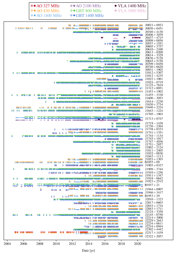
Figure 1: Epochs of all TOAs in the data set. The observatory and observing frequency are indicated by color: Arecibo observations are red (327 MHz), orange (430 MHz), light blue (1.4 GHz), and purple (2.1 GHz); GBT observations are green (800 MHz) and dark blue (1.4 GHz); and VLA observations are brown (1.4 GHz) and pink (3 GHz). The Arecibo and GBT data acquisition systems are indicated by symbols: open circles are ASP or GASP, and closed circles are PUPPI or GUPPI. Only a single backend (YUPPI) was used at the VLA.

Data were collected using the GBT, Arecibo, and the VLA. A summary of the observing systems can be found in Table 1. The maximum timing baseline for an individual pulsar in this data release is 16 years. GBT and VLA data through 2020 April 4 are included in this data set, corresponding to the last date when the GUPPI backend on the GBT was used. Arecibo data are included through 2020 August 10, the date of the first cable breaking at Arecibo and the end of regular observations using the telescope. Of the 68 MSPs in NG15, 30 MSPs with declinations $0^{\circ}<\delta<+39^{\circ}$ were solely observed with Arecibo, and 31 MSPs with $\delta>-45^{\circ}$ (and outside the declination range accessible to Arecibo) with the GBT. Two pulsars, PSRs J1713+0747 and B1937+21, were observed with the GBT, Arecibo, and the VLA; PSRs J1600$-$3053, J1643$-$1224, and J1909$-$3744 were observed at both the GBT and the VLA; PSR J1903+0327 was observed with Arecibo and the VLA; and PSR J0437$-$4715 was observed only at the VLA.

We adhered to a roughly monthly cadence in our observations: every $\sim$ three weeks at Arecibo and four weeks at the GBT and VLA. As described in NG12, with the GBT and Arecibo we additionally performed high-cadence observations (every $\sim$ five days) of six of the highest timing precision pulsars for increased sensitivity to single sources emitting continuous GWs. There were some interruptions in data-taking, in particular: telescope painting at Arecibo and azimuth track refurbishment at the GBT in 2007, earthquake damage at Arecibo in 2014, and a brief pause in observing at Arecibo following Hurricane Maria in 2017. The transition from test observations to incorporating new MSPs into our regular observing campaign at the GBT looks like a gap in data collection for those pulsars in early 2017. The lack of Arecibo data in 2018 is due to an instrumental issue described further in Section A.2.

Each MSP was observed with at least two widely-separated frequencies at each epoch (with a few exceptions), with the observing frequencies for a given pulsar chosen to maximize its timing precision. At Arecibo, MSPs were observed at 430 MHz and 1.4 GHz or at 1.4 GHz and 2.1 GHz. Several Arecibo pulsars were observed at all three frequencies (Table 5) and PSR J2317+1439 was originally observed at 327 and 430 MHz, but was migrated to 430 MHz and 1.4 GHz at roughly the midpoint in its timing baseline. At the GBT, all MSPs were observed at 820 MHz and 1.4 GHz. The VLA is expected to provide improved sensitivity and frequency coverage in the 2–4 GHz range, so it was used for 3-GHz observations of five MSPs predicted to give optimal timing precision at these frequencies (Lam et al., 2018a): PSRs J1713+0747, J1600$-$3053, J1643+1224, J1903+0327, and J1909$-$3744. The VLA was additionally used for dual-frequency (1.4 and 3 GHz) observations of PSR J0437$-$4715, a very bright MSP that lies just below the declination range accessible to the GBT, and for PSR J1713$+$0747. The latter is observed at 1.4 GHz with all three telescopes in order to provide a cross-check for possible instrumental systematics. The exceptions to dual-frequency observations were the high-cadence observations at the GBT, which were carried out at only 1.4 GHz but with a large bandwidth.

At Arecibo and the GBT, over the course of our experiment we have used two generations of data acquisition instrumentation (i.e., pulsar “backends”). For the first approximately six years, the ASP and GASP instruments with 64 MHz bandwidth (Demorest, 2007) were used to acquire data from Arecibo and the GBT respectively, after which we transitioned to PUPPI (Puerto Rican Ultimate Pulsar Processing Instrument; at Arecibo, in 2012) and GUPPI (Green Bank Ultimate Pulsar Processing Instrument; at the GBT, in 2010). The PUPPI and GUPPI backends processed bandwidths of up to 800 MHz (DuPlain et al., 2008) and provided significantly improved timing compared to ASP and GASP. Simultaneous observations using both generations of instruments were used to measure offsets between the old and new backends (Appendix A of NG9), and we continue to include these offsets in our timing models as we have in previous data releases. The YUPPI backend was used to acquire all VLA data in this data release. The resulting raw data consist of folded, full-Stokes pulse profiles, with 2048 pulse phase bins, radio frequency resolution of 4 MHz (ASP/GASP), $\sim$ 1.5 MHz (GUPPI/PUPPI) or 1 MHz (YUPPI), and sub-integrations of 1 s (with PUPPI at 1.4 and 2.1 GHz) or 10 s (with all other receiver/back-end pairings). Hereafter, if a description applies to all three of the GUPPI, PUPPI, and YUPPI backends, we will refer to them in shorthand as the “UPPI backends.”

VLA observations employed the “phased array” mode of telescope operation. In this mode, the voltage data streams of the individual antennae are coherently added, resulting in a single data stream with properties roughly equivalent to those of a single dish of equal total collecting area. This summed signal is then subdivided into frequency channels, coherently dedispersed, and folded in the same manner as typical single-dish pulsar data. The final results are data products (folded profiles) that in subsequent processing can be treated identically as single-dish data. In order to maximize sensitivity of the array sum, radio-wave phase fluctuations due to atmospheric variations across the array must be corrected in real time. During observations, phase corrections were measured using a bright continuum calibrator, typically within $\sim$5 deg of the target pulsar, and applied to the data. This re-phasing process was repeated every 10 minutes.

For all telescopes/backends, at the start of each pulsar observation, a pulsed noise-diode signal was injected in order to later calibrate the pulsar signal amplitude during the data reduction steps. For GUPPI and PUPPI data, the noise signal amplitude was calibrated into equivalent flux density units (i.e., Janskys) approximately monthly using on/off observations of an unpolarized continuum radio source of known flux density. Details about the continuum sources can be found in Section 8 of NG12. For the VLA with YUPPI, this second flux-calibration step was not done, and the resulting data are scaled in units relative to the noise diode power.

Table 1: Observing Frequencies and Bandwidths

	Backends
	ASP/GASP					PUPPI/GUPPI/YUPPI
Telescope		Frequency	Usable	$\Delta$DM			Frequency	Usable	$\Delta$DM
Receiver	Data Span	Range	Bandwidth	Delay		Data Span	Range	Bandwidth	Delay
		[MHz]	[MHz]	[$\mu$s]			[MHz]	[MHz]	[$\mu$s]
Arecibo
327	$2005.0-2012.0$	$315-339$	34	2.86		$2012.2-2020.6$	$302-352$	50	6.00
430	$2005.0-2012.3$	$422-442$	20	1.03		$2012.2-2020.6$	$421-445$	24	1.23
L-wide	$2004.9-2012.3$	$1380-1444$	64	0.09		$2012.2-2020.6$	$1147-1765$	600	0.91
S-wide	$2004.9-2012.6$	$2316-2380$	64	0.02		$2012.2-2020.6$	$1700-2404$	460	0.36
GBT
Rcvr_800	$2004.6-2011.0$	$822-866$	64	0.30		$2010.2-2020.3$	$722-919$	180	1.52
Rcvr1_2	$2004.6-2010.8$	$1386-1434$	64	0.07		$2010.2-2020.3$	$1151-1885$	640	0.98
VLA
1.5GHz	$\cdots$	$\cdots$	$\cdots$	$\cdots$		$2015.2-2020.3$	$1026-2014$	800	1.46
3GHz	$\cdots$	$\cdots$	$\cdots$	$\cdots$		$2015.3-2020.0$	$2012-3988$	1700	0.38

3 Data Reduction and Times-of-Arrival Generation

3.1 Data Reduction and Procedure

We followed a standardized process to use the raw data files to calculate calibrated profiles and TOAs. Some steps can be iterative in nature; for example, initial timing must be done before an analysis identifying outlying TOAs. With this caveat in mind, we list the steps that we took to produce science-ready pulse profiles and to generate TOAs from those profiles:

1. Exclusion of known bad/corrupted files or time ranges. From previous data sets, we were already aware of a number of data files that were not suitable for inclusion in the data set due to various instrumental issues. In addition, in newer data contributing only to NG15, there is a $\sim 10$-month time range with unusable Arecibo data (see Section A.2). We excluded all of these files from NG15.

2. Artifact removal. This step removes artifacts from the interleaved analog-to-digital converter (ADC) scheme used by the UPPI receivers to achieve their wide bandwidths. The artifacts appear as negatively dispersed pulses and impact TOA generation if not removed. Details about these artifacts and their removal are given in Section 2.3.1 and Figure 2 of NG12.

3. Radio frequency interference excision and calibration. We performed the standard radio frequency interference (RFI) excision and calibration procedures detailed in NG11, with the additional step of excising RFI from the calibration files along with the data files as described in Section 2.3.2 of NG12.

4. Time- and frequency-averaging. Details for Arecibo and GBT data are given in Section 3.1 of NG9. The UPPI data were frequency-averaged (“scrunched”) into 1.6 to 32 MHz-bandwidth channels, depending on the receiver. ASP/GASP data were not averaged, and remained at the native 4 MHz resolution. The cleaned, calibrated profiles were time-averaged into sub-integrations of up to 30 minutes. For the few pulsars with very short binary periods, we time-averaged into sub-integrations no longer than 2.5% of the orbital period.

5. TOA generation. This process is described in Section 3.2, with further details in NG9 and NG11; details for wideband-specific TOA generation can be found in NG12WB and references therein.

6. Outlier analysis of TOA residuals. The automated process by which we identified and removed outlier TOA residuals is described in Section A.4.

7. Further, often iterative, data cleaning. Further data quality checks and cleaning are described in Section 3.3.

Steps 2–5 were performed using the nanopipe data processing pipeline (Demorest, 2018). This in turn uses the PSRCHIVE pulsar data analysis software package (Hotan et al., 2004) to perform most of the processing steps outlined here, plus PulsePortraiture for wideband template generation and TOA measurement (Pennucci et al., 2016). All software package versions and specific data processing settings used in this analysis, along with the resulting TOA data (step 5), were tracked in a git-based version control repository (“toagen”). A version tag and corresponding git hash linking the TOA to a specific git commit are included in the final TOA lines, allowing a complete description of the TOA provenance to be reconstructed as needed.

3.2 Time-of-Arrival Generation

TOAs are derived from folded pulse-profile data by measuring the time shift of the observed profile relative to a model pulse shape for each pulsar, known as a template; this basic approach has been standard in pulsar timing analyses for decades (e.g., Taylor, 1992). This data release includes both narrowband and wideband TOAs, as did NG12. In the narrowband approach, a separate TOA is measured for each frequency channel, at the final time and frequency resolution described in Section 3.1, step 4; dispersion measure (DM) is fit to these TOAs along with other timing parameters. In the wideband approach, a single TOA and DM value are measured for the full receiver band, using a frequency-dependent template (also called a portrait) that accounts for pulse shape evolution (for details, see Pennucci et al., 2014).

All narrowband template profiles used in this data set were regenerated from the UPPI data, using the procedures described in NG5. All profiles for a given pulsar and receiver band are aligned, weighted by signal-to-noise ratio, and summed to create a final average. This average profile is then “denoised” using wavelet decomposition and thresholding. The process is iterated several times to converge on the final template. All narrowband TOAs, including those from ASP and GASP data, were then generated using this set of templates using procedures described in more detail in NG9 and NG11. As in NG12, we used an improved algorithm to calculate TOA uncertainties, in which we numerically integrate the TOA probability distribution (Equation 12 in Appendix B of NG9) to mitigate underestimation of uncertainties for low S/N TOAs.

Wideband template portaits were created following NG12WB. Again, all data for a given pulsar and receiver are aligned and summed, while in this case preserving (rather than averaging over) frequency channels. The final average portrait is then modeled and denoised as described in Pennucci (2019) to create a template that preserves profile evolution with frequency. For the 47 MSPs in NG12, we re-used the previous GUPPI and PUPPI wideband templates from that analysis. New templates were generated for the YUPPI data and the 21 pulsars new to the present data set. New wideband TOAs for all data were then generated as described in NG12WB.

3.3 Cleaning the Data Set for Improved Data Quality

In Section 2.5 of NG12, we detailed a number of steps taken to improve the quality of our data set. Many of the same steps were taken in this data set as well, in particular the following data cuts (and corresponding NG12 sections): S/N cut (2.5.1), bad DM range cut (2.5.2), outlier residual TOA cut (2.5.3, except a different method was used in the present work, as described in Appendix A.4 below), epoch $F$-test cut (2.5.7), and orphan data cut (2.5.9). The corrupt calibration cut (NG12 Section 2.5.5) was not explicitly repeated in this data set, but the files that were cut from the NG12 were also cut from NG15. Manual removal of individual TOAs or data files was done similarly as in NG12 Sections 2.5.4 and 2.5.8, with some differences, so these cuts are described below in Appendix A.5.

Table 2 summarizes each of the cuts used in NG15, including the order in which they were applied, and the number of TOAs affected by each cut in the narrowband and wideband data sets respectively. After all TOA cutting was complete, the final narrowband data set had 676,465 TOAs (34.6% cut) and the wideband data set had 20,290 TOAs (21.6% cut).

Table 2: TOA Removal Flags

Flag	Reason for TOA Removal	$N_{\rm nb}$	$N_{\rm wb}$
Initial Cuts (Loading TOAs)
-cut simul	ASP/GASP TOA taken at the same time as a PUPPI/GUPPI TOA	6,883	648
-cut orphaned	Insignificant data volume ($\leq 3$ epochs for a given receiver band; usually test observations)	2,837	13
-cut badrange	Arecibo data affected by malfunctioning local oscilator (MJDs 57984–58447)	56,658	2,036
-cut snr	Profile data used to generate TOA does not meet signal-to-noise ratio threshold ($\mathrm{S/N}_{\rm nb}<8$ and $\mathrm{S/N}_{\rm wb}<25$)	255,118	1,324
-cut poorfebe	Poor quality data from given frontend/backend combination	512	5
-cut eclipsing	For pulsars showing signs of eclipses, TOAs near superior conjunction (within $10-15\%$ of an orbital phase) were automatically excised	4,551	109
-cut dmx	Ratio of maximum to minimum frequency in an observing epoch (in a single DMX bin) $f_{\rm{max}}/f_{\rm{min}}<1.1$	13,006	1,086
Initial Totals		339,565	5,221
Automated Outlier Analysis
-cut outlier10	TOA has outlier probability $p_{i,{\rm out}}>0.1$	5,374	–
-cut maxout	Entire file removed if a significant percentage ($>8\%$) of TOAs flagged as outliers	5,072	–
-cut epochdrop	Entire epoch removed with epochalyptica(), based on an $F$-test $p$-value $<10^{-6}$	6,027	188
Auto Totals		16,473	188
Manual Cuts (Human Inspection)
-cut badtoa	Remaining TOAs identified by human inspection and removed	249	1
-cut badfile	Remaining files identified by human inspection and removed	1,163	170
Manual Totals		1,412	171
Removed TOAs		357,450	5,580
Remaining TOAs		676,465	20,290

Note. — The flags are listed here in the order in which they were applied in our final pipeline run. A single cut flag is assigned to each TOA that is removed. Narrowband and wideband data sets were analyzed independently.

4 Timing Analysis

From the outset, our goal was to produce a self-consistent data set consisting of human-readable configuration (yaml) files, which produced standard timing model parameter (.par) files for each pulsar. Aside from the parameter values themselves, configuration files contain all necessary information to reproduce timing results and the files are organized to facilitate using version control to track any changes made along the way. All timing fits used the JPL DE440 solar system ephemeris (Park et al., 2021) and the TT(BIPM2019) timescale.

As in NG12, we used standardized Jupyter notebooks (Kluyver et al., 2016) to automate our timing procedures and we built new software tools to improve transparency, code readability, and reproducibility of our results. Our analysis pipeline is now entirely PINT-based (Luo et al., 2021) — previous releases used TEMPO (Nice et al., 2015) — and flexible enough to accommodate working with both narrowband and wideband TOAs. A frozen version of code used to produce NG15 results as well as intermediate data products can be found at data.nanograv.org (see Section 4.5 for more details). An open source version of our timing analysis package, PINT_Pal, is also available.

4.1 Timing Models and Parameters

Pulsar timing requires determination of the TOAs and comparison to a model composed of many different physical effects. Our timing parameter sets fall into six categories, with the numbers of parameters in each category fit per pulsar shown in Table 6.

1. Spin: We fit three parameters describing the rotational phase, frequency, and frequency derivative of each pulsar. In one case (long-period binary PSR J1024$-$0719), we also fit the second frequency derivative.

2. Astrometry: For each pulsar we fit five parameters describing the two-dimensional position on the sky in ecliptic coordinates, the two-dimensional proper motion, and parallax. As in our previous works, we fit all five of these regardless of the measurement significance.

3. Binary: For 50 of our observed systems we fit binary parameters describing the orbit with a companion star. With the exception of the long-period binary PSR J1024$-$0719, we fit, at a minimum, the five Keplerian parameters fully characterizing the orbit. Several different models were used depending on the orbital characteristics, see Section 4.1.1.

4. Dispersion Measure: Time-variations in the DM require that we fit the TOAs with a dispersive delay proportional to $\nu^{-2}$ and the unknown DM at that epoch. This is discussed in greater depth in Section 4.2.

5. Frequency dependence: Additional time-independent but frequency-dependent delays are fit for on a per-pulsar basis (“FD” parameters; see NG9), with the number included determined via our $F$-test procedure discussed below in Section 4.1.2. In the narrowband data, we take these to describe time offsets due to differences in the observed pulse shape at a given frequency compared to the template shape used in timing. In the wideband data, we expect the pulse portrait to encapsulate the changing frequency-dependence of the profiles. However, we still find several significant FD parameters. We fit for these values in the same manner regardless, and the significance of these will be explored more in future work. Though the physical mechanism has not been definitively determined, other time-varying chromatic processes could be picked up as time-independent FD parameters.

6. Jump: We fit for “jumps” to account for unknown phase offsets between data observed by different receivers and/or telescopes.

4.1.1 Binary Models

We used one of five binary models, depending on the orbital characteristics of the pulsar in question. Low-eccentricity orbits (see Section 5.1.3) were fit using the ELL1 (Lange et al., 2001) or ELL1H (Freire & Wex, 2010) model, depending on whether or not Shapiro delay was marginally detected; orbits with higher eccentricity were modeled with the BT (Blandford & Teukolsky, 1976) or DD (Damour & Deruelle, 1985, 1986; Damour & Taylor, 1992) model; and for PSR J1713+0747, in which we measure the physical orientation of the orbit, we used the DDK model (Kopeikin, 1996). Pedagogical descriptions of these binary models can be found in Lorimer & Kramer (2012). In all cases, at a minimum we included and fit five Keplerian parameters in the binary model: the orbital period $P_{b}$ or orbital frequency $f_{b}$; the projected semimajor axis $x$; and either the eccentricity $e$, longitude of periastron $\omega$, and epoch of periastron passage $T_{0}$ in the DD or DDK models, or two Laplace-Lagrange parameters ($\epsilon_{1},\epsilon_{2}$) and the epoch of the ascending node $T_{\mathrm{asc}}$ in the ELL1 or ELL1H models.

The ELL1 model describes the orbit with the Laplace-Lagrange eccentricity parameterization, with $\epsilon_{1}=e\sin{\omega}$ and $\epsilon_{2}=e\cos{\omega}$ (for a more complete description of this parameterization, see Lange et al., 2001). This parameterization is needed because for a nearly circular orbit, one cannot reliably define the time and location of the periastron. If the Shapiro delay was marginally detected via the $F$-statistic as described below, we instead modeled low-eccentricity orbits with the ELL1H model, which is simply the ELL1 model with the addition of the $h_{3}$ and $h_{4}$ parameters from the orthometric Shapiro delay parameterization of Freire & Wex (2010). For a significant detection of Shapiro delay, the companion mass $m_{c}$ and orbital inclination $\sin{i}$ parameters were instead included in the ELL1 model.

The BT and DD models directly measure $e$, $x$, and $T_{0}$, and are more accurate than the ELL1 model for orbits with a large enough eccentricity to measure the longitude and epoch of periastron. The BT model is Newtonian, while the DD model is a theory-independent relativistic model that allows for the inclusion of Shapiro delay parameters, companion mass $m_{c}$ and inclination angle via $\sin{i}$. In our data set, the use of ELL1 and DD is split nearly evenly between pulsars. For one of our most precisely-timed pulsars, PSR J1713+0747, we found in NG12 that we were sensitive to the annual-orbital parallax (Kopeikin, 1995), which allows the true orientation of the orbit to be measured. Thus we transitioned from the DD to DDK model for this pulsar. The DDK model incorporates the orbital inclination and the longitude of the ascending node of the orbit, $\Omega_{\mathrm{asc}}$ (Kopeikin, 1996). Appendix B describes our use of the DDK model in detail.

For the majority of orbital models, we used the orbital period $P_{b}$, but for four short orbital period ($P_{b}<0.5$ d) pulsars we instead included the orbital frequency $f_{b}$ in the model. Using the orbital frequency instead of period allows us to include multiple orbital frequency derivatives to better describe the orbit, rather than being restricted to only the first period derivative if using $P_{b}$; it also allows us to easily test for additional derivatives using the $F$-statistic. All four of these pulsars are in “black widow” systems (Swihart et al., 2022). Three of them are non-eclipsing (PSRs J0023+0923, J0636+5128, and J2214+3000), while PSR J1705$-$1903 eclipses for $\approx$ 30% of each 4.4-hr orbit.

All four of these pulsars’ orbits are low-eccentricity and were modeled with the ELL1 model. For PSR J2214+3000, only $f_{b}$ (“FB0” in the timing model) was needed, with no derivatives; J0636+5128 required three derivatives (FB0 through FB3); and J0023+0923 and J1705$-$1903 required five derivatives (FB0 through FB5).

In all cases, we tested for the presence of the Shapiro delay using the $F$-statistic, as described in Section 4.1.2 below. If $m_{\mathrm{c}}$ and $\sin{i}$ were significantly detected, we added these parameters to the timing model and re-fit.

4.1.2 Parameter Inclusion and Significance Testing Criteria

As in NG12 and our prior data releases, an $F$-statistic was used to determine what additional parameters should be included in the timing model beyond those describing pulsar spin, astrometry, red and white noise, and Keplerian binary motion. This test is valid in the case that one model is a subset of another; therefore, these tests were performed by fitting a nominal model, recording the resulting $\chi^{2}$, then adding or subtracting the parameter of interest and re-fitting. The $F$-statistic is:

$$F=\frac{(\chi^{2}_{0}-\chi^{2})/(n_{0}-n)}{\chi^{2}/n}$$ (1)

where $\chi^{2}_{0}$ and $n_{0}$ are the best-fit chi-squared value and number of degrees of freedom, respectively, for the nominal (superset) model. Parameters were included if they induced a $p<0.0027$ ($\sim$3$\sigma$) change in the fit. As described in NG12, this test was applied to secularly-evolving binary parameters ($\dot{P}_{\text{b}}$, $\dot{\omega}$, and $\dot{x}$), Shapiro delay parameters, frequency-dependent (FD; see NG9) parameters, and higher-order orbital frequency derivatives (FB$n$, where $n=0$ corresponds to the orbital frequency and $n=\{1,2,...\}$ correspond to frequency derivatives) where applicable. For parameters with components of increasing complexity (like FD1-5, where a model cannot include non-contiguous combinations of parameters), the test was applied iteratively. All FB and FD terms below the highest-order term that induced a significant change in the fit were included, even if a subset of the lower-order parameters did not produce a significant change; for example, if FD3 is significant but FD2 is not, then FD1, FD2, and FD3 are included in the model. The summary plots generated with PINT_Pal provide the user with suggestions for parameters to add or exclude in the model.

4.2 Dispersion Measure Variations

Changes in the Earth-pulsar line of sight require that we account for variations in the DM on short (i.e., per-epoch) timescales (Jones et al., 2017). We measure the pulsar signals over a wide range of radio frequencies to estimate the time-varying DM for both narrowband and wideband data sets (see Figure 1). We used the DMX model, a piecewise constant function, to describe these variations, with each DMX parameter describing the offset from a nominal fixed value. Modeling of these variations requires up to hundreds of additional parameters (see Table 6), and for most of our pulsars the expected variations from interstellar turbulence alone are significant enough between epochs that we cannot reduce the number of parameters (Jones et al., 2017).

At Arecibo and the VLA, observations with different receivers were consecutive whereas with the GBT one or more days passed between observations for scheduling efficiencies. We assumed a constant value for the DM over a window of time 0.5 days long for any pulsars with Arecibo observations and longer windows for pulsars solely observed with the GBT, with a 15-day range for GASP data and 6.5-day range for GUPPI/YUPPI data. If the maximum-to-minimum frequency ratio of the TOAs did not satisfy $\nu_{\rm max}/\nu_{\rm min}>1.1$, we excised the data as described above and did not fit a DMX parameter.

Besides DM variations due to the turbulent interstellar medium, another visually-apparent contribution is from the Earth-pulsar line of sight intersecting different sections of the solar wind. For a few specific pulsars close to the ecliptic plane, the change in DM can be significant even within the time range of a single window. We use the following criterion to find such windows. As in NG11 and NG12, for this purpose, we used a toy model of a spherically-symmetric and static solar wind electron density given by $n_{e}(r)=n_{0}(r/r_{0})^{-2}$ where $r$ is the distance from the Sun and $n_{0}=5~{}\mathrm{cm}^{-3}$ is the fiducial electron density at a distance $r_{0}=1$ au (e.g., Splaver et al., 2005). If the projected DM variation due to the change in the line of sight through the solar wind would have induced a timing variation of greater than 100 ns, the DMX time ranges were divided into 0.5-day windows, with data still subject to the frequency cut described above. Note that this toy solar wind model is used only for this test while setting DMX window sizes; it is not included in the pulsar timing models themselves. Thus reported DMX values in the timing models incorporate dispersion by both the solar wind and the interstellar medium.

In addition to being our most-observed pulsar, PSR J1713+0747 experienced rapid chromatic variations over a period of several months in 2016 (e.g. Lam et al., 2018b; Chen et al., 2021; Goncharov et al., 2021) such that it was necessary to split the DMX windows to avoid additional excess timing noise from the event as in NG12. Following the conclusion of the current data set, PSR J1713+0747 experienced a profile change, first reported in Xu et al. (2021), confirmed by Meyers & Chime/Pulsar Collaboration (2021), and further discussed by Singha et al. (2021) and Jennings et al. (2022). As this event occurred outside of the range of data reported here, we do not need to correct for it in this release.

4.3 Noise Modeling

Pulsar timing uses a phenomenological noise model for the data that is separated into two broad components distinguished by the time scale of the correlations between the TOAs. The white noise (WN) model, i.e., noise that is uncorrelated in time and hence spectrally flat, inflates the values of the TOA uncertainties, $\sigma_{\rm S/N}$, derived from the pulse template matching process (Taylor, 1992). The template matching process assumes that the data are a scaled and shifted version of the pulse profile, however other sources of noise can be best modeled as WN, but do not come from the template matching process (Lommen & Demorest, 2013).

Our noise modeling paradigm is discussed in detail in NG15detchar, and briefly summarized here. Three WN parameters – EFAC ($\mathcal{F}$), EQUAD ($\mathcal{Q}$) and ECORR ($\mathcal{J}$) – are used to adjust TOA uncertainties in order to accurately represent the WN present in the data. EFAC scales TOAs linearly, accounting for uncertainty induced by template matching errors or template mismatches. For well-characterized systems, EFAC tends to 1.0. EQUAD adds an additional WN in quadrature, ensuring a minimum error size. ECORR also adds in quadrature and accounts for uncertainty that is correlated among frequencies within an observation, most importantly pulse jitter, though other mechanisms can add as well (Lam et al., 2017).

Various differences between pulsar timing backends and radio observatory receivers (e.g., the frequency ranges covered) make it necessary to give different values of these WN parameters to each receiver/backend combination. These WN terms come together with receiver/backend combination, $re/be$, dependence as

$$C_{ij}=\mathcal{F}^{2}(re/be)[\sigma_{{\rm S/N},i}^{2}+\mathcal{Q}^{2}(re/be)]\;\delta_{ij}+\mathcal{J}^{2}(re/be)\;\mathcal{U}_{ij}$$ (2)

where the $i,j$ denote TOA indices across all observing epochs, $\delta_{ij}$ is the Kronecker delta and we omit the dependence on receiver and backend, $re/be$, from here on for simplicity. While EFAC and EQUAD only add to the diagonal of $C$, where $C_{ij}$ are the elements of the covariance matrix, the ECORR terms are block diagonal for single observing epochs. ECORR is modeled using a block diagonal matrix, $\mathcal{U}$, with values of $1$ for TOAs from the same epoch and zeros for all other entries.

Pulsar timing data often show evidence of correlations across longer timescales than can easily be modeled with ECORR terms. These correlations are instead modeled as a single stationary Gaussian process with a power-law spectrum

$$P(f)=A_{\rm red}^{2}\left(\frac{f}{1~{}\mathrm{yr}^{-1}}\right)^{\gamma_{\rm red}},$$ (3)

where $f$ is the Fourier frequency, $\gamma_{\rm red}$ is the spectral index, and $A_{\rm red}$ is the noise amplitude at a reference frequency of 1 yr^-1. Long-timescale correlated data are characterized as red noise (RN) in which $\gamma_{\rm red}<0$. ECORR is not separately modeled in the wideband data set, as it is completely covariant with EQUAD.

The timing model and noise analysis are performed iteratively over each pulsar data set, first fitting a preliminary pulsar ephemeris and then doing a Bayesian noise analysis with ENTERPRISE using a linearized timing model (see Section 4.4 below for details about the linearized version of the timing model). We then refit the timing model with the noise parameters obtained from ENTERPRISE. This process is repeated until the timing and noise parameters stabilize and noise posteriors look nearly identical from one run to the next. Slight changes from NG12 in the implementation of the Bayesian noise analysis include increasing the number of samples obtained and matching the prior for the spectral index to those used in the GW detection pipeline.

The WN parameters EFAC, EQUAD, and ECORR are measured for each pulsar-backend-receiver combination. A small fraction of these WN parameters changed by $>$ 3 $\sigma$ between NG12 and NG15 (28/159, 17/159, and 5/159 for EFAC, EQUAD, and ECORR, respectively). Even so, these changes are not unexpected as the length of the data set increases, especially for pulsars that were newly added to NG12.

Twenty-three pulsars in NG15 were found to have significant levels of RN. Ten of these measurements are newly significant in NG15, while 13 of the 14 sources with significant RN in NG12 continued to favor its inclusion in their timing models. Only PSR J2317+1439, which favored an $A_{\rm red}$ an order of magnitude lower than the next-lowest $A_{\rm red}$ in NG12, as well as a steep $\gamma_{\rm red}$ comparable to that of PSR J0030+0451, had RN parameters removed from its timing model in NG15. No $\gamma_{\rm red}$ or $A_{\rm red}$ values differed between the data sets by more than a factor of $\sim$ 3 $\sigma$ for pulsars with significant RN in both NG12 and NG15.

4.4 Linearity Testing for Pulsar Timing Models

A pulsar timing model is a deterministic function $t^{\rm det}$ that takes parameter values $\mathbf{p}$ and predicts observed pulse phases at the time of each TOA $t^{\rm obs}$ (in time units) such that the observed TOAs are the deterministic values plus noise $n$, i.e., $t^{\rm obs}=t^{\rm det}(\mathbf{p}_{\rm true})+n$. We are able to simplify our GW detection calculations by using a linear approximation to this function (Ellis et al., 2013):

$$r(\mathbf{p}_{\rm best})\equiv t^{\rm obs}-t^{\rm det}(\mathbf{p}_{\rm best})\approx\left.\frac{\partial t^{\rm det}(\mathbf{p}_{\rm true})}{\partial\delta\mathbf{p}}\right|_{\delta\mathbf{p}=0}\delta\mathbf{p}+n,$$ (4)

where $\mathbf{p}_{\rm best}$ is our vector of best-fit parameters from our generalized least-squares fit which form our residuals $r$, and $\delta\mathbf{p}\approx\mathbf{p}_{\rm true}-\mathbf{p}_{\rm best}$ is therefore small. The term with the partial derivative on the right-hand side is the design matrix. One generally expects this approximation to be good when the data constrain the parameters tightly, relative to the level of non-linearity intrinsic to each parameter; for example, some are entirely linear. Since this level varies significantly between different parameters in the model, we developed tests to verify that the approximation of linearity is adequate.

In our reported models, the parameter uncertainties and the parameter correlations define an ellipsoid. If the linear model is adequate, then the plausible pulsar parameter values are constrained by the data to lie within or near this ellipsoid. Thus this ellipsoid is the region where we require the timing model to be well approximated by the linearized model. While we generally use analytical marginalization with flat priors to remove the (linearized) timing model parameters from the GW detection process, we expect that most samples from preliminary detection Markov chains will fall within or near this error ellipsoid (Kaiser et al. in prep). Thus we try to test the degree to which the full timing model differs from its linearized approximation over this error ellipsoid.

One direct approach is simply to shift the value of each parameter, one at a time, by one sigma from the best-fit $\mathbf{p}_{\rm best}$. For each parameter, this produces a trial parameter set $\mathbf{p}_{\rm trial}$, from which we then compute the difference in residuals $r(\mathbf{p}_{\rm trial})-t^{\rm det}(\mathbf{p}_{\rm trial})$ (in time units). This provides a measurement of the deviation from linearity for this parameter at the time of each TOA. In the case of highly covariant parameters this approach may result in $\mathbf{p}_{\rm trial}$ falling outside the full (multi-dimensional) error ellipse. Therefore, this test can be considered a conservative upper limit on the level of non-linearity; the true level may be lower. For each pulsar and parameter we checked whether the root-mean-squared amplitude of this deviation was less than 100 ns. We found only a few parameters on a few pulsars that exceeded this threshold. The most common example was the time ($T_{0}$) and longitude ($\omega$) of periastron. These two parameters form part of an essentially polar representation of the orbital shape, and when the orbit is nearly circular this coordinate system introduces nonlinearities; for the pulsars where this was a problem the nonlinearity was typically on the scale of a few microseconds. A second cause for nonlinearity is the parameter $\sin i$, which is constrained by the Shapiro delay. The shape of the Shapiro delay as a function of orbital phase is quite nonlinear in the parameter $\sin i$, and so for pulsars where the Shapiro delay is poorly constrained this nonlinearity introduces a few-microsecond discrepancy.

For the pulsars and parameters where nonlinearities appear in the above test, we carried out a more stringent test. Since the detection tools analytically marginalize the timing parameters, any discrepancy that can be modeled as a linear combination of the timing model derivatives disappears. We therefore evaluated each of the problem cases, removing all such components. The discrepancy that remains is not absorbed during Bayesian fitting. This process resolved nearly all of the above nonlinearities, with the following exceptions: the parameter $\sin i$ for the pulsars J1630+3734, J1811$-$2405, J1946+3417, J2017+0603, and J2302+4442, and the parameters $\sin i$, $P_{b}$, $\dot{\omega}$, $\omega$, and $T_{0}$ for the pulsar J1630+3734. For the parameter $\sin i$, in each case the three-sigma confidence interval extends above the physical limit of 1, so nonlinearities must be expected. They take the form of a sharp peak around superior conjunction, and are mostly about 1 microsecond. PSR J1630+3734 is a pulsar with only three years of data, and because of the orbital coordinate system, its $P_{b}$ is highly correlated with $\dot{\omega}$, along with the nonlinearities we observe in other pulsars with nearly-circular orbits. The discrepancies in this case are of the order 10 microseconds.

The conclusion of this analysis is that the vast majority of pulsar parameters in our data set can be very well approximated by a linearized model, therefore applying this approximation when marginalizing over the timing model as part of GW analyses is not a significant source of error. For the small number of parameters that may show significant nonlinearity, the effect occurs at the pulsar’s orbital period. These are generally days to weeks so are unlikely to interfere with the GW signals of interest on timescales of years. The main result of nonlinearity is that parameter uncertainties estimated from the linearized model are potentially unreliable. For these parameters additional analysis is required to determine posterior probability distributions; refer to Sec. 5.1.4 for discussion of Shapiro delay measurements and pulsar masses in our results.

4.5 Data Products

Our complete catalog of observations for 68 millisecond pulsars is available alongside this publication at https://data.nanograv.org. We also provide metadata and other useful intermediate files generated from pipeline runs there, including:

• Configuration (*.yaml) files,

• Standardized pulsar parameter (*.par) files,

• Initial TOA (*.tim) files,

• TOA files with cut flags applied (*excise.tim),

• Noise modeling chains and parameter files,

• DMX timeseries (*dmxparse*.out).

For ease of use, timing models will be made available in both Tempo2 (Hobbs & Edwards, 2012) and PINT formats. In addition, the correlation matrices for fit parameters of all pulsars are provided in the following formats:

• Human-readable list of pairwise correlations (*.txt),

• Machine-readable NumPy compressed correlation matrices (*.npz),

• Standardized HDF5 compressed correlation matrices (*.hdf5).

Finally, we have containerized the production environments utilized in the production of NG15. The following options will be released alongside the NG15 data set:

• An interactive Docker (Merkel, 2014) container, which is built off of the Official Jupyter images to ensure compatibility with the JupyterHub software stack (Granger & Pérez, 2021).

• A Singularity (Kurtzer et al., 2017) container, which is optimized for HPC workloads.

• An Anaconda Environment, consisting of Conda-Forge (conda-forge Community, 2015) packages tested against Python 3.10.

5 Timing Model Comparisons & Newly Measured Parameters

5.1 Comparison of NG12 and NG15 Timing Models

The careful analysis of changes to timing model parameters can provide a wealth of secondary science results and provide a measure of confidence in additions to the data set. Here, we present a basic summary of changes between the 12.5 and 15-year data releases, focusing specifically on improvements in astrometric and binary parameter measurements, changes in WN and RN parameters, and discrepancies between timing solutions obtained with Tempo2 and PINT.

5.1.1 Astrometric Parameter Comparison

Figure 2: Measurements and uncertainties of parallax from the 12.5-yr and the current 15-yr data sets, showing the parallax values to be consistent across data sets. Orange Xs denote the NG12 measurement, while blue circles denote the NG15 measurement. Horizontal lines of the corresponding color mark the extent of the 1-$\sigma$ measurement uncertainty. The timing algorithm allows both positive and negative parallaxes, even though only positive values are physically meaningful. As expected, none of the negative parallax values are significant within their uncertainties.

We begin by comparing the astrometric parameters, specifically the parallax and proper motion values.

We are particularly interested in NG15 parameters that have changed by $>3\sigma_{12.5}$ relative to NG12, where $\sigma_{12.5}$ is the $1-\sigma$ uncertainty on the NG12 parameter (i.e. a conservative estimate of a 3$\sigma_{12.5}$ discrepancy). We find three pulsars with $>3\sigma_{12.5}$ changes in the ecliptic longitude component of proper motion $\mu_{\lambda}$ (PSRs J0636+5128, $3.5\sigma_{12.5}$; J1909$-$3744, $3.7\sigma_{12.5}$; and J1946+3417, $7.0\sigma_{12.5}$), and one pulsar with a $>3\sigma_{12.5}$ change in parallax (PSR J0023+0923, $3.4\sigma_{12.5}$). It is known that variations in the red noise parameters, orbital parameters, and other parameters that require long timescales for measurement have covariances with astrometric parameters, such that a few pulsars will have $\gtrsim 3\sigma$ changes in some of these parameters. Such covariances can therefore explain the changes in astrometric parameters between NG12 and NG15. For example, PSR J1946+3417 has red noise in NG15, but not in NG12, explaining the change in proper motion; and the measured parallax of PSR J0023+0923 changes significantly with the addition or removal of orbital frequency derivatives in its timing model.

In all cases, the uncertainty on the 15-yr parameter is smaller than that of the 12.5-yr, as is expected for a parameter measured with a longer data set. Figure 2 shows the 12.5- and 15-yr parallax values for all pulsars that were included in both data sets.

5.1.2 Comparison of Narrowband & Wideband Timing Models

As in NG12 and NG12WB, we have generated both a narrowband and a wideband data set as part of the NG15 process. However, it is critical to note that the wideband data set is not being used to derive any GW background or astrophysical interpretation-related results. Its primary purpose is to aid in refining the techniques used in wideband TOA generation and in the curation of wideband timing solutions in order to prepare for the eventual inclusion of data from wide-bandwidth receivers and cope with prohibitively large narrowband data volumes in future releases. In this work, the wideband data set is only used to derive preliminary pulsar masses for sources with significantly measured Shapiro delay parameters (see 5.1.3).

A thorough comparison of all measured parameters common between the narrowband and wideband timing solutions for each source was conducted, as in NG12WB. In that work, few discrepancies larger than 2 $\sigma_{12.5}$ were found. However, the longer NG15 wideband data set has shown a handful of discrepancies that are currently under investigation. In several cases, either the length of the wideband or the narrowband data set is sufficiently long (due to automatic outlier excision in the other data set) to significantly measure RN. In others, either the data set length or presence of RN caused a parameter (usually orbital) to be included in one of the data sets, but not both. Covariances between (usually orbital) parameters as discussed in Section 4.4 may also worsen these discrepancies. For example, a barely-significant measurement of the relativistic Shapiro delay would require the addition of the two post-Keplerian parameters that describe the effect. However, if the constraint is not strong, nonlinearities in binary orbital parameters may exacerbate discrepancies in these parameter measurements. In general, these covariances might lead to larger possible discrepancies in narrowband and wideband parameter constraints. The overall impact of these discrepancies is minimal, as the only analysis referencing the wideband data set is the preliminary measurement of pulsar masses. Further refinement of this procedure will proceed the publication of the next NANOGrav data release.

5.1.3 Binary Model Comparison

The high cadence and long timing baseline of NANOGrav’s data set enables the detailed study of a large number of MSP binary systems. NG9 and its accompanying publication Fonseca et al. (2016), as well as NG11 and NG12, have included analyses of binary sources timed as part of the NANOGrav PTA. In this work, we present a basic overview of newly measured binary parameters, changes to timing models, and new constraints on pulsar masses from the measurement of post-Keplerian Shapiro delay orbital parameters. A manuscript describing our more in-depth analysis of the 15-year binary sources is in preparation.

Of the 68 MSPs included in the current data set, 50 are in binary systems. Because these sources are selected for their high timing precision and stability, the vast majority are in near-circular orbits with white-dwarf companions. Of the 21 new MSPs added since NG12, 18 are binaries. As more observations are added to the data set, sensitivity to secular binary parameters (i.e., $\dot{x}$, $\dot{\omega}$, and $\dot{P_{\text{b}}}$) improves. Additionally, parameters such as the relativistic Shapiro delay can be more precisely measured with better orbital phase coverage. We see a number of improvements and changes to binary parameter measurements resulting from the addition of $\sim$3 years of NANOGrav observations.

Consistency between the narrowband and wideband data sets is discussed in 5.1.1. Any discussion regarding the addition and removal of parameters, as well as their values, are based on the narrowband NG12 and 15-year data sets. However, because the wideband data set consists of significantly fewer TOAs (the NG12WB data volume is $\sim$33 times smaller than that of NG12), mass determinations based on post-Keplerian parameter measurements are based on the wideband data set to reduce computational burden.

Discrepant binary parameters: Several NANOGrav MSPs have shown significant changes ($>3\sigma$) in measured Keplerian orbital parameters since NG12, as determined by the absolute value of the difference in parameter value between NG12 and now, divided by the NG12 uncertainty. However, these $>3\sigma$ discrepancies can generally be explained by changes to the pulsar’s orbital or RN model.

For example, the significance of $P_{b}$ for PSR J1600$-$3053 decreased since NG12  primarily due to the addition of RN, a new measurement of $\dot{\omega}$, and an added frequency-dependent parameter (FD3). Relative to the recent, larger uncertainty, the value of $P_{b}$ increased by 4.3 $\sigma$. Newly measured RN in PSR J1614$-$2230 (one of the highest-mass neutron stars known; see Demorest et al., 2010) was accompanied by a 3.8 $\sigma$ increase in $P_{b}$.

Such changes are plausible as the PTA timing baseline increases and sensitivity to long-term orbital variations improves. Because secular evolution of parameters can happen on timescales similar to those of intrinsic RN, these two measurements can be covariant (see NG12).

Ten of the 50 binary sources show newly measured values for either $\dot{P_{\text{b}}}$, $\dot{x}$, or $\dot{e}$ (see Table 3). In the case of PSR J0613$-$0200, $\dot{x}$ was removed and $\dot{P_{\text{b}}}$ was added.

Changes to binary models: Because the ELL1 binary model is only valid for sufficiently circular orbits, a test ($a\,\text{sin}(i)\,e^{2}/c\ll\sigma_{\mathrm{S/N}}/N_{\mathrm{TOA}}^{1/2}$; see Appendix A1 of Lange et al. 2001) was imposed on all ELL1 binaries to ensure its validity. ELL1 is no longer valid for PSR J1918$-$0642, so this source is now parameterized by the DD binary model.

The sources PSR J1853+1303 and PSR J1918$-$0642 required changes to their binary models as a result of the increased length of the data set; specifically, we have chosen to use the DD binary model instead of ELL1H and ELL1 for PSRs J1853+1303 and J1918$-$0642, respectively (see Table 3). PSR J1853+1303 was discussed in detail in NG12 because the orthometric Shapiro delay parameters $h_{\text{3}}$ and $h_{\text{4}}$ were newly constrained. We now significantly measure the traditional Shapiro delay parameters $m_{\text{c}}$ and $\sin i$ as determined by an $F$-test comparison; therefore, the DD parameterization is merited. Although these parameters are significantly measured, we do not yet meaningfully constrain the pulsar mass ($m_{\text{p}}=3.3^{+12.3}_{-2.6}$ $M_{\odot}$; see Section 5.1.4). Continued observations will result in improved orbital coverage, potentially enabling a more precise $m_{\text{p}}$ measurement in future data releases.

5.1.4 Pulsar Masses from the Relativistic Shapiro Delay

Because an extensive analysis of each of the 50 binary MSPs included here is beyond the scope of this data release, a more in-depth manuscript detailing our binary analysis similar to NG9 and Fonseca et al. (2016) is in preparation. Here, we present pulsar mass ($m_{\text{p}}$) measurements obtained from measurement of the relativistic Shapiro delay in cases where the companion mass ($m_{\text{c}}$) and orbital inclination angle ($i$) are significantly constrained. When these two parameters are combined with the Keplerian mass function and the extremely well-determined $x$ and $P_{b}$ orbital parameters, the pulsar’s mass and companion mass can be measured independently. In the rare case that other post-Keplerian parameters can also be constrained, one’s ability to precisely measure $m_{\text{p}}$ is improved; however, our basic analysis does not take this additional information into account.

Posterior probability distribution functions (PDFs) for pulsar masses (see Figure 3) were derived from grid-based iteration over $m_{\text{c}}$ and sin($i$) using PINT. For each combination of $m_{\text{c}}$ and $\sin i$, a $\chi^{2}$ fit was performed without holding other model parameters (except the measured WN and RN values) fixed. Equations 4 and 5 and associated text in Fonseca et al. (2016) explain the Bayesian translation (with uniform priors) from this $\chi^{2}$ grid to marginalized posterior PDFs in $m_{\text{c}}$ and $\sin i$ in greater detail. While Fonseca et al. (2016) and Fonseca et al. (2021) (hereafter, FCP21) perform the $\chi^{2}$ model fits using Tempo2, the PINT-based results presented here were cross-checked with Tempo2-derived results. For assumed white-dwarf companions with poorly-constrained masses, grids spanned the 0–2 $M_{\odot}$ range. All inclination angles (sampled uniformly in $\cos i$ rather than $\sin i$ to represent a random distribution of orbital orientations) were searched if that parameter was not already well constrained. Unless otherwise noted, reported uncertainties correspond to 68.3% confidence intervals, and grids were 200 by 200 samples in size.

Two of the 18 binary MSPs added to the NANOGrav data set since NG12, PSRs J1630+3734 and J1811$-$2405, show (according to the $F$-test) significantly — if not precisely — measured Shapiro delay (see Table 4). We measure the mass of PSR J1630+3734 to be $6.7^{+5.0}_{-2.9}$ $M_{\odot}$. While this mass is intriguingly high, this source has only three years of timing data and suffers from nonlinearities in multiple of its measured binary parameters (see Section 4.4). PSR J1811$-$2405 suffers from the same limitations and nonlinear tendencies as PSR J1630+3734. A lengthened timing baseline will help resolve some of these covariances and improve our constraint of $m_{\text{p}}$.

A number of factors determine the precision of Shapiro delay measurements. Among these are the density of observational coverage around superior conjunction, a pulsar’s timing precision and noise characteristics, and its orbital geometry. A number of $m_{\text{p}}$ measurements have improved between NG12 and the current data release, due in part to a longer timing baseline and improved orbital coverage (see Figure 3 and Table 4). The 68.3% $m_{\text{p}}$ confidence intervals for PSRs J0740+6620, J1600$-$3053, and J1741+1351, improved by a factor of $>2.5$ between NG12 and the present work.

PSR J0740+6620 is of particular interest to those wishing to constrain the poorly understood dense matter equation of state (EoS), as the measurement of unprecedentedly high-mass neutron stars provides support for a subset of “stiff” EoS. Timed by NANOGrav since 2014, this source is one of the most massive neutron stars known. Cromartie et al. (2020) reported its mass to be $2.14^{+0.10}_{-0.09}$ $M_{\odot}$ after a series of follow-up campaigns around superior conjunction with the GBT. FCP21 provided an updated measurement of its mass, $2.08^{+0.07}_{-0.07}$ $M_{\odot}$, after combining the aforementioned follow-up observations with a preliminary NG15 and daily-cadence Canadian Hydrogen Intensity Mapping Experiment pulsar observing system (CHIME/Pulsar; CHIME/Pulsar Collaboration et al., 2021) observations. Radio-derived neutron star mass constraints can be employed as priors in mass-to-radius measurements from X-ray lightcurve modeling (e.g., Riley et al., 2021 and Miller et al., 2021).

This work demonstrates that based on NANOGrav observations alone, the mass of PSR J0740+6620 is constrained $>$7 times better by NG15 compared to NG12, an improvement that can be attributed to the orbital-phase-targeted campaigns first presented in Cromartie et al. (2020) and the additional $\sim$3 years of regular NANOGrav observations. However, this analysis does not incorporate the high-cadence CHIME data, nor does it take into account the newly measured $\dot{P}_{\text{b}}$ (which is dependent on $m_{\text{c}}$, $m_{\text{p}}$, and the distance $d$ to the source), or optimized dispersion measure modeling as FCP21 does. We therefore do not regard the present measurement, which is consistent with the FCP21 to within 1$\sigma$, as superseding that result.

PSR J1614$-$2230, the first directly observed 2-$M_{\odot}$ neutron star (Demorest et al., 2010), is timed as part of the NANOGrav PTA. In this data release, the addition of newly measured RN to its timing model coincides with a $\sim$1-$\sigma$ increase in $m_{\text{p}}$.

Conducting orbital-phase-specific observing campaigns around superior conjunction results in demonstrated improvements in $m_{\text{p}}$ constraints for sufficiently highly-inclined systems. For this reason, five MSPs currently timed by NANOGrav that show borderline $m_{\text{p}}$ constraints (including PSRs J1630+3734, J1811$-$2405, and J1853+1303) were subject to such a targeted GBT campaign in spring 2022, the results of which will be included in a future manuscript.

Table 3: Binary Models & Binary Model Changes for MSPs common to NG12 and NG15

Source	Binary Model	New Parameters	Removed Parameters
J0023+0923	ELL1	FB5	-
J0613-0200	ELL1	$\dot{P_{\text{b}}}$	$\dot{x}$
J0636+5128	ELL1	FB2, FB3	-
J0740+6620	ELL1	$\dot{P_{\text{b}}}$	-
J1012+5307	ELL1	$\dot{x}$	-
J1125+7819	ELL1	$\dot{x}$	-
J1455-3330	DD	-	-
J1600-3053	DD	$\dot{\omega}$	-
J1614-2230	ELL1	-	-
J1640+2224	DD	$\dot{e}$	-
J1643-1224	DD	$\dot{e}$	-
J1713+0747	DDK	-	-
J1738+0333	ELL1	-	-
J1741+1351	ELL1	$\dot{P_{\text{b}}}$	-
J1853+1303	ELL1H to DD	-	-
B1855+09	ELL1	-	-
J1903+0327	DD	-	-
J1909-3744	ELL1	-	-
J1910+1256	DD	-	-
J1918-0642	ELL1 to DD	$\dot{x}$	-
J1946+3417	DD	-	-
B1953+29	DD	-	-
J2017+0603	ELL1	-	-
J2033+1734	DD	-	-
J2043+1711	ELL1	$\dot{P_{\text{b}}}$	-
J2145-0750	ELL1H	-	-
J2214+3000	ELL1	-	-
J2229+2643	DD	-	-
J2234+0611	DD	$\dot{P_{\text{b}}}$	-
J2234+0944	ELL1	-	-
J2302+4442	DD	-	-
J2317+1439	ELL1H	-	-

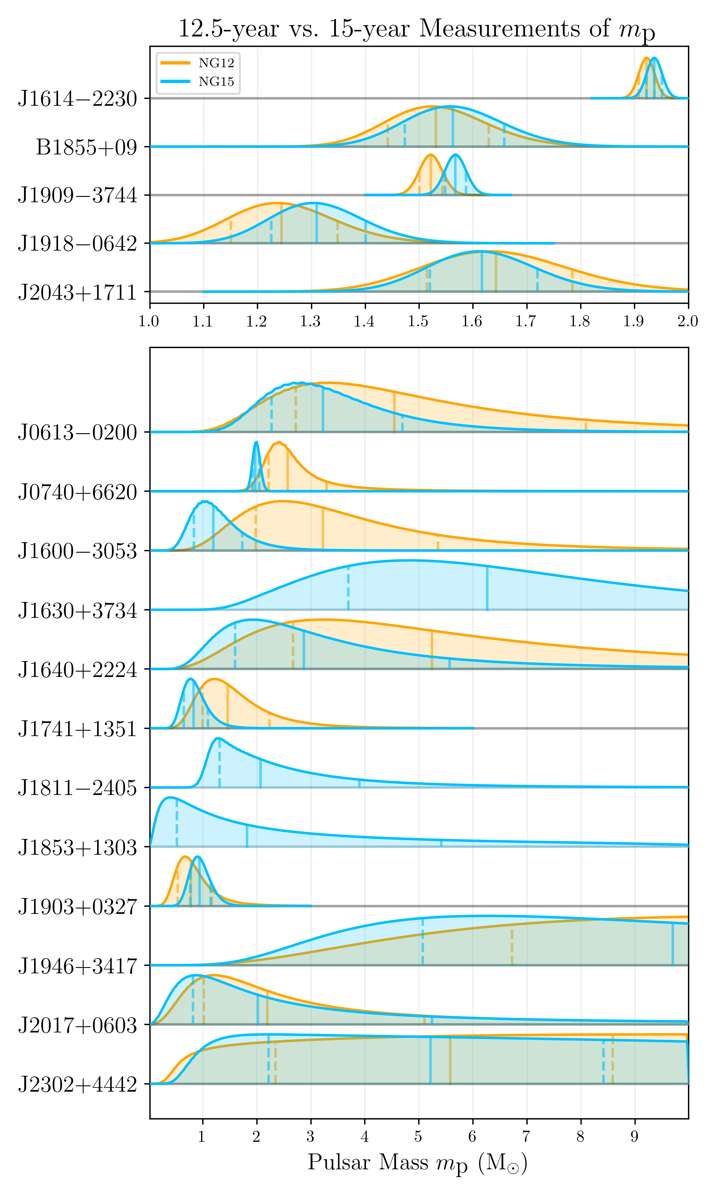
Figure 3: Posterior probability distributions for pulsar mass $m_{\text{p}}$ for each NG15 binary with well-constrained traditional Shapiro delay parameters. Solid lines within the PDF curves indicate the median mass value, while the two dotted lines represent the 68.3% confidence interval. Orange curves were derived using NG12 measurements; blue curves are from the updated NG15 data set. Of the 14 Shapiro delay measurements common to NG12 and NG15, seven of the mean masses decreased, while seven either increased or did not appreciably change.

Table 4: Shapiro delay-derived Mass Measurements

Source	NG12 $m_{\text{p}}$ ($M_{\odot}$)	NG15 $m_{\text{p}}$ ($M_{\odot}$)	$\sigma$ change
J0613$-$0200	$4.5^{+3.5}_{-1.8}$	$3.2^{+1.4}_{-0.9}$	$-0.5\,\sigma$
J0740+6620	$2.57^{+0.73}_{-0.35}$	$1.99^{+0.07}_{-0.07}$	$-1.1\,\sigma$
J1600$-$3053	$3.2^{+2.1}_{-1.2}$	$1.20^{+0.54}_{-0.36}$	$-1.2\sigma$
J1614$-$2230	$1.922^{+0.015}_{-0.015}$	$1.937^{+0.014}_{-0.014}$	$+1.0\sigma$
J1630+3734	-	$6.3^{+4.2}_{-2.6}$	-
J1640+2224	$5.2^{+5.0}_{-2.6}$	$2.8^{+2.3}_{-1.2}$	$-0.6\sigma$
J1741+1351	$1.5^{+0.77}_{-0.46}$	$0.83^{+0.26}_{-0.19}$	$-1.0\sigma$
J1811$-$2405	-	$2.1^{+1.8}_{-0.76}$	-
J1853+1303	-	$1.8^{+3.6}_{-1.3}$	-
B1855+09	$1.531^{+0.098}_{-0.089}$	$1.563^{+0.095}_{-0.089}$	$+0.3\sigma$
J1903+0327	$0.78^{+0.39}_{-0.24}$	$0.94^{+0.21}_{-0.17}$	$+0.5\sigma$
J1909$-$3744	$1.52^{+0.022}_{-0.021}$	$1.57^{+0.020}_{-0.019}$	$+2.2\sigma$
J1918$-$0642	$1.24^{+0.10}_{-0.09}$	$1.31^{+0.09}_{-0.08}$	$+0.7\sigma$
J1946+3417	$3.9^{+0.8}_{-1.1}$	$3.9^{+0.8}_{-1.1}$	$0\sigma$
J2017+0603	$2.2^{+2.9}_{-1.2}$	$2.0^{+3.2}_{-1.2}$	$0\sigma$
J2043+1711	$1.64^{+0.14}_{-0.13}$	$1.62^{+0.10}_{-0.10}$	$-0.2\sigma$
J2302+4442	$5.6^{+3.0}_{-3.2}$	$5.2^{+3.2}_{-3.0}$	$-0.1\sigma$

5.1.5 Changes in Noise Parameters Since the 12.5-Year Data Set

Section 4.3 and the detector characterization paper (NG15detchar) describe the WN and RN modeling conducted for each pulsar in the data set. A small fraction of WN parameters (28/159, 17/159, and 5/159 for EFAC, EQUAD, and ECORR, respectively) changed by $>3\sigma$ between NG12 and NG15. Even so, these changes are not unexpected as the length of the data set increases, especially for pulsars that were newly added to NG12.

Twenty-three pulsars in NG15 were found to have significant levels of RN (see solid points in Figure 4). Ten of these measurements are newly significant in NG15, while 13 of the 14 sources with significant RN in NG12 continued to favor inclusion of RN in their timing models. Only PSR J2317+1439, which favored RN amplitude an order of magnitude lower than the next-flattest spectral index in NG12, as well as a steep spectral index comparable to that of PSR J0030+0451, had RN parameters removed from its timing model in NG15. RN parameter values for pulsars with RN in both NG12 and NG15 were checked for consistency. No spectral index or amplitude values differed between the data sets by more than a factor of just over $\sim$3$\sigma$. Not only are these inconsistencies small, but they are also expected to accompany a growing data set.

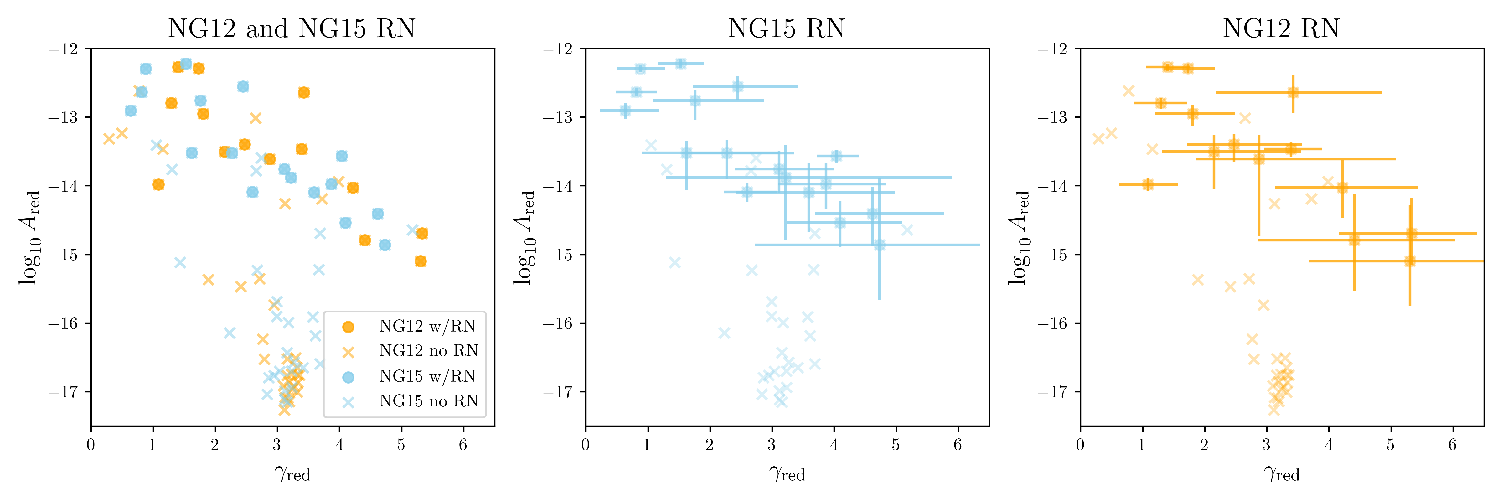
Figure 4: Comparisons of the two RN parameters (the spectral index $\gamma_{\rm red}$ and $\log_{10}$ amplitude, $\log_{10}A_{\rm red}$) between NG15 and NG12. Left: $\log_{10}A_{\rm red}$ vs. $\gamma_{\rm red}$ for NG15 (blue) and NG12 (orange) without error bars. Solid square points are values for pulsars whose RN was found to be significant and is included in the timing model. Crosses are the measured RN parameters for pulsars without significant RN. Middle, right: The same plot, split into the NG15 values (middle) and NG12 values (right), including the 1-$\sigma$ confidence interval error bars. For crosses (insignificant RN) appearing in the “high-$A_{\rm red}$” group of points, the RN priors are the only information constraining those measurements; that is, the data provide no information about the RN content of those MSPs.

5.1.6 Kopeikin Parameter Analysis for PSR J1713+0747

Unlike the majority of the binary systems analyzed here, for PSR J1713+0747 we need to use the DDK model that incorporates the effects of proper motion and parallax on the binary orbit (Kopeikin, 1995, 1996, and see Appendix B). However, in addition to the convention ambiguity discussed in Appendix B, the nature of the analysis in Kopeikin (1996) also leads to further ambiguity with nearly similar solutions possible for different choices of inclination $i$ and longitude of the ascending node $\Omega$. These are locations where the change in projected semi-major axis $\delta x$ is equal to the best-fit value, but where $\delta\dot{x}$ is different. The locations of these points can be found by first determining where $\delta\dot{x}$ is 0, which is where:

$$\Omega=\Omega_{0}\equiv\tan^{-1}\left(\frac{\mu_{\beta}}{\mu_{\lambda}}\right)$$ (5)

(defined in ecliptic coordinates). With an initial best-fit pair $(i,\Omega)$ the other points can then be identified as:

$$i,\Omega=\left\{\begin{array}[]{cc}i&\Omega\\ i&2\Omega_{0}-\Omega-180{\arcdeg}\\ 180{\arcdeg}-i&\Omega+180{\arcdeg}\\ 180{\arcdeg}-i&2\Omega_{0}-\Omega\end{array}\right.$$ (6)

We wished to verify that the solution we had settled on was in fact a global and not just a local minimum. To do this we computed a grid of $\chi^{2}$ over values of $(i,\Omega)$ with PINT, with all other parameters freely fit at each grid point. We used a preliminary version of the narrow-band TOAs for this purpose, but subsequent changes and comparison with wide-band TOAs did not indicate any difference.

We stepped through all values of $\Omega$ from $-180\arcdeg$ to $+180\arcdeg$ in $1\arcdeg$ increments, and similarly stepped through values of $i$ from $0\arcdeg$ to $180\arcdeg$ in $1\arcdeg$ increments. As mentioned in Appendix B our final fit with PINT used ecliptic coordinates, but we wished to compare to results from the literature that were done in equatorial coordinates. The value of $i$ will not change, but the value of $\Omega$ will change. However, at this location in the sky the equatorial (ICRS) and ecliptic coordinate systems are almost aligned, with $\Omega_{\rm ICRS}=\Omega_{\rm Ecliptic}-5.3\arcdeg$.

The results of this fit are shown in Figure 5. The four local minima given by Equation 6 are clearly visible, and we actually found that our initial fit had ended up in the wrong local minimum. However we have now verified that the minimum identified by our non-linear fitter is the global minimum, with $\chi^{2}$ differences of 261 to 904 for the alternatives (with approximately 59000 degrees of freedom).

This also agrees with the solutions from Splaver et al. (2005) and Alam et al. (2021a), once they have been corrected to use the Damour & Taylor (1992, hereafter DT92) convention for defining $\Omega$ (Appendix B) and ecliptic coordinates, again verifying that we have found the global minimum. We note that the Alam et al. (2021a) result was derived using the T2 timing model, and that the resulting values of $\Omega$ and $i$ may be shifted from the values found by the other models by roughly $0.1\sigma$, due to the use of unadjusted Keplerian parameters in computing binary delays (see Appendix B).

Finally, we also get the same result if we fit using Tempo and convert from the IAU to DT92 convention for defining $\Omega$ (Appendix B).

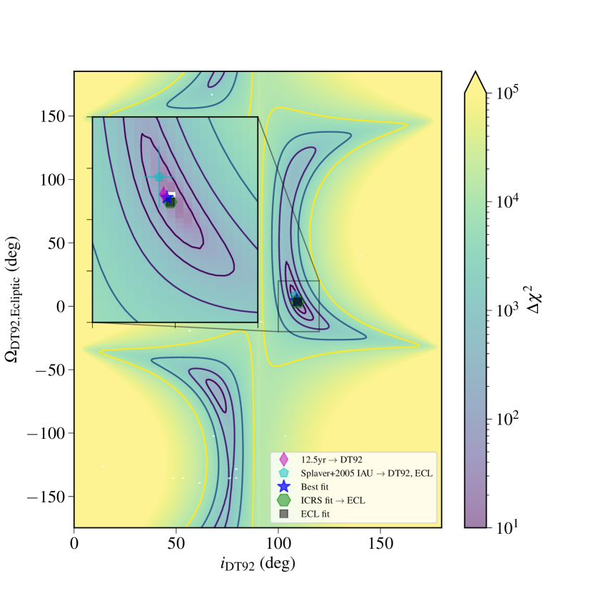
Figure 5: Grid of $\chi^{2}$ as a function of inclination $i$ and longitude of the ascending node $\Omega$ for PSR J1713+0747, computed with PINT. All other parameters were fit at each grid point. The values are in the Damour & Taylor (DT92; 1992) convention (see Appendix B). The color scale and contours are the logarithm of difference of $\chi^{2}$ compared to the best-fit value, with an inset zooming in to the best-fit region. The magenta diamond is the value from the 12.5 yr data release (Alam et al., 2021a) converted from the IAU convention to DT92; these parameters will be slightly shifted due to the choice of timing model. The cyan pentagon shows the value from Splaver et al. (2005) converted from the IAU convention to DT92, and additionally converted from equatorial to ecliptic coordinates. The green hexagon is the best-fit when using equatorial coordinates, converted to ecliptic. The black square is the best-fit when using ecliptic coordinates directly. Finally the blue star is the minimum point in the $\chi^{2}$ grid.

5.2 Comparison of Split-Telescope Data Sets

Most pulsars in the data set are observed by only one observatory, either GBT or Arecibo. However, two pulsars are observed by both GBT and Arecibo (PSR B1937+21 and PSR J1713+0747) and several are observed with the VLA in addition to GBT or Arecibo.

For pulsars observed with GBT and Arecibo, we create timing solutions using TOAs from each telescope separately, in addition to the combined data set, and compare respective parameters. These data sets enable separate GBT and Arecibo “split-telescope” gravitational wave background searches, as in NG15gwb. Equally important, we use these separate data sets to check consistency between observatories. As both telescopes have extensive data sets for PSR B1937+21 and PSR J1713+0747, we expect the solutions to be statistically consistent with each other and with the combined solution. Comparisons of these solutions have confirmed that this is the case.

Additionally, for pulsars observed with the VLA and Arecibo (J1903+0327) or the VLA and GBT (J1600-3053, J1643-1224, and J1909-3744), we create separate Arecibo or GBT-only data sets. Due to the small number of TOAs, we do not create VLA-only data sets for these sources. We again compare the Arecibo or GBT only solution to the complete solution. In all cases, we find parameters are consistent within $3-\sigma$, except where differences in the systems used, data spans, frequency ranges, or RN parameters would make changes expected.

6 New Pulsars

Since the 12.5-year data set, many new MSPs are now being observed and results for 21 new pulsars are included in NG15. Historically, NANOGrav has had a close relationship with pulsar survey groups using the Arecibo and Green Bank Observatories and in NG15, new sources came from three un-targeted surveys at these telescopes, the Arecibo 327 MHz Drift-Scan Pulsar Survey (PSRs J0509+0856 and J0709+0458; Martinez et al., 2019), the Pulsar Arecibo L-band Feed Array survey (PSR J0557+1551; Scholz et al., 2015), and the Green Bank North Celestial Cap survey (PSR J0406+3039). Four more came from targeted surveys at Arecibo/Green Bank, guided by Fermi Large Area Telescope (LAT) unassociated $\gamma$-ray sources (PSRs J0605+3757, J1312+0051, J1630+3734, and J0614$-$3329; Sanpa-Arsa, 2016; Ransom et al., 2011). We also draw on discoveries from similar targeted surveys carried out with the Parkes Telescope (PSR J1012$-$4235; Camilo et al., 2015) and the Effelsberg Telescope (PSR J1745+1017; Barr et al., 2013) and additional blind surveys like the High Time Resolution Universe Survey (PSRs J1705$-$1903, J1719$-$1438, and J1811$-$2405; Morello et al., 2019; Ng et al., 2014) and the Parkes Multibeam Pulsar Survey (PSR J1802$-$2124; Faulkner et al., 2004), which both use the Parkes Telescope. Some sources added here are also monitored by the EPTA (PSRs J1751$-$2857 and J1843$-$1113; Desvignes et al., 2016) and the PPTA (PSR J0437$-$4715; Reardon et al., 2021). PSRs J0610$-$2100, J1022+1001, J1730$-$2304, and J2124$-$3358 are also monitored by both EPTA and PPTA. While seemingly redundant, overlap in observing programs among regional PTAs like this is useful for International Pulsar Timing Array (IPTA) data combination and for diagnosing related issues (e.g., see Hobbs et al., 2010; Perera et al., 2019). Overlap in observing programs can enhance our frequency coverage and cadence for these pulsars as well.

7 Summary and Conclusions

In this paper we have presented the 15-year data set from the NANOGrav collaboration, using data from the Green Bank, Arecibo, and VLA telescopes. Our longest timing baselines have increased by $\sim$3 yr over our previous data set. Even more impactful is the increase in the number of pulsars, from 47 MSPs in the 12.5-year data set to 68 MSPs in the present data set; this is the largest fractional increase ($\sim$50%) in the number of pulsars since the size of the array doubled between NG5 and NG9. This large increase was made possible by NANOGrav’s push to evaluate many new MSPs discovered in large-area sky surveys and targeted gamma-ray-guided surveys; it is notable because a PTA’s sensitivity to a GWB increases linearly with the number of pulsars in the array and as the square root of the overall timing baseline (Siemens et al., 2013).

Another high-impact addition in this data set is the novel pipeline, PINT_Pal   that automates the timing process. The user interfaces with a configuration file to set up the run by specifying which TOA files, noise chains, etc. to use, and the pipeline runs the timing analysis and outputs a series of diagnostic plots and tables with which the user determines whether or not the full timing model is sufficient. The timing analysis can easily be re-run by editing the configuration file, e.g. to conduct iterative noise analyses when parameters are added or removed from a given pulsar’s timing model. This pipeline lowers the bar of entry for students and others who are relatively new to pulsar timing, and it will be of great use in future data sets, especially as the number of pulsars continues to grow. The intent is for this pipeline to also be adapted and used by other PTA collaborations and for more general pulsar timing analysis and IPTA data combination. The publicly available PINT_Pal can be found at https://github.com/nanograv/pint_pal.

In NG12, we included a comparison between the Tempo and PINT timing results. A thorough comparison between timing software was also included in Luo et al. (2019). In the 15-yr data set, we have shifted to using PINT as the primary timing software. PINT is a modular, python-based software, and this transition decreases barriers to entry in understanding our pipeline and results. In NG12, we conducted systematic comparisons between Tempo and PINT, demonstrating the consistency of our prior and current timing software.

In Section 5, we performed a number of comparisons: we compared the astrometric, binary, and RN parameters measured in the 12.5-yr and 15-yr data sets, and the timing and RN parameter results between individual-telescope data sets for those pulsars observed with both Arecibo and GBT. Overall, the parameters are consistent between the various data sets. A small number of parallax, proper motion, and mass measurements have changed significantly between the 12.5-yr and 15-yr data releases, as detailed in Sections 5.1.1 and 5.1.3. In NG12, we reported detectable levels of RN for 14 pulsars; in the 15-yr data set we measure RN for 23 pulsars, 13 of which were also found to show RN in NG12. Aside from the one source for which we detected RN in NG12 but not in the 15-yr, RN parameters were consistent between the data sets.

NANOGrav continues to be committed to public data releases for GW detection, as well as for individual pulsar studies. In addition, we are committed to data-sharing and collaborative analysis within the IPTA, of which the EPTA, InPTA, and PPTA are also members. NG15, along with the most recent EPTA, InPTA, and PPTA data sets, have already been shared with the IPTA in order to create a combined data set, which will be more sensitive to GW signals than any individual PTA data set. IPTA data combination analyses have begun.

We are also committed to continuing to increase the size of the NANOGrav PTA. The loss of Arecibo was significant, as new faint pulsars that fall in its declination range can no longer be added to the array, and we have been unable to continue observing a small number of faint pulsars previously observed at Arecibo. Despite this, NANOGrav will continue to evaluate new MSPs for inclusion in our GBT, VLA, and CHIME timing campaigns. With the proposed DSA-2000 telescope (Hallinan et al., 2019), NANOGrav will further expand its timing campaign, increasing the number of MSPs observed and thus our sensitivity to GWs.

Author contributions.

The alphabetical-order author list reflects the broad variety of contributions of authors to the NANOGrav project. Some specific contributions to this paper, particularly incremental work between NG12 and the present work, are as follows.

JKS and MED coordinated Arecibo observations. PBD, JKS, and KSt coordinated GBT observations. PBD and KSt coordinated VLA observations. ZA, PRB, PTB, HTC, MED, PBD, TD, ECF, EF, WF, DCG, PAG, MLJ, JL, MTL, DRL, RSL, AMc, MAM, NM, CN, NSP, TTP, SMR, ASc, BJS, IHS, JKS, and KSt each ran at least 10 sessions and/or 20 hours of observations for this project. MFA, VB, CC, CJ, AK, YL, KM, EP, LS, and SK led observing programs run by undergraduate teams. AMA, BSA, AB, HTC, PBD, DCG, JG, NG, RJJ, MTL, DJN, NSP, TTP, and JKS developed and refined procedures and computational tools for the timing pipeline. AMA, HTC, RJJ, DLK, MK, JL, AMc, PSR, SMR, ASu, BJS, and JKS coordinated and implemented PINT development to facilitate NG15 analysis. JKS coordinated development of the data set. AA, GA, AMA, PRB, HTC, KC, MED, PBD, EF, WF, DCG, JG, NG, MLJ, RJJ, MK, JL, MTL, MAM, AMc, BWM, DJN, BBPP, NSP, TTP, HAR, PSR, SMR, BJS, CS, IHS, JKS, and HMW generated and checked timing solutions for individual pulsars. JKS coordinated the writing of this paper. HTC and TTP also aided in coordination of data analyses and paper writing. PBD wrote observing proposals and performed calibration and TOA generation. PBD and TTP developed wideband portraits to generate corresponding TOAs. HTC, JG, NSP, and JKS implemented and performed outlier analyses and data quality checks described in Section 3.3. GEF, AJ, SRT, and QW assisted in implementing the outlier analysis code into the timing pipeline. NSP and JSH assisted in interpreting the noise modeling results. NSP undertook comparisons between PINT, Tempo, and Tempo2 results. DLK and IHS aided in comparisons specifically related to Kopeikin parameters, as described in Section 5.1.6. MED performed the comparison of astrometric parameters between data sets. HTC, KC, and JKS performed comparisons between the narrowband and wideband data sets. HTC and EF undertook analysis of binary systems. DCG compared split telescope results for the subset of pulsars observed with multiple telescopes. Significant contributors to the text, tables, and figures in this paper include HTC, MED, PBD, DCG, JG, JSH, DLK, MTL, MAM, DJN, SMR, IHS, and JKS. HTC produced the timing residual plots. JG and NG oversaw and maintained much of the computational infrastructure related and essential to this work and contributed to the design and public release of the PINT_Pal code repository. We dedicate this paper to our wonderful colleague Jing Luo, whom we lost this past year.

The NANOGrav collaboration receives support from National Science Foundation (NSF) Physics Frontiers Center award numbers 1430284 and 2020265, the Gordon and Betty Moore Foundation, NSF AccelNet award number 2114721, an NSERC Discovery Grant, and CIFAR. The Arecibo Observatory is a facility of the NSF operated under cooperative agreement (AST-1744119) by the University of Central Florida (UCF) in alliance with Universidad Ana G. Méndez (UAGM) and Yang Enterprises (YEI), Inc. The Green Bank Observatory is a facility of the NSF operated under cooperative agreement by Associated Universities, Inc. The National Radio Astronomy Observatory is a facility of the NSF operated under cooperative agreement by Associated Universities, Inc. This work was conducted using the Thorny Flat HPC Cluster at West Virginia University (WVU), which is funded in part by National Science Foundation (NSF) Major Research Instrumentation Program (MRI) Award number 1726534, and West Virginia University. This work was also conducted in part using the resources of the Advanced Computing Center for Research and Education (ACCRE) at Vanderbilt University, Nashville, TN. NANOGrav is part of the International Pulsar Timing Array (IPTA); we would like to thank our IPTA colleagues for their help with this paper.

L.B. acknowledges support from the National Science Foundation under award AST-1909933 and from the Research Corporation for Science Advancement under Cottrell Scholar Award No. 27553. P.R.B. is supported by the Science and Technology Facilities Council, grant number ST/W000946/1. S.B. gratefully acknowledges the support of a Sloan Fellowship, and the support of NSF under award #1815664. M.C. and S.R.T. acknowledge support from NSF AST-2007993. M.C. and N.S.P. were supported by the Vanderbilt Initiative in Data Intensive Astrophysics (VIDA) Fellowship. Support for this work was provided by the NSF through the Grote Reber Fellowship Program administered by Associated Universities, Inc./National Radio Astronomy Observatory. Support for H.T.C. is provided by NASA through the NASA Hubble Fellowship Program grant #HST-HF2-51453.001 awarded by the Space Telescope Science Institute, which is operated by the Association of Universities for Research in Astronomy, Inc., for NASA, under contract NAS5-26555. K.C. is supported by a UBC Four Year Fellowship (6456). M.E.D. acknowledges support from the Naval Research Laboratory by NASA under contract S-15633Y. T.D. and M.T.L. are supported by an NSF Astronomy and Astrophysics Grant (AAG) award number 2009468. E.C.F. is supported by NASA under award number 80GSFC21M0002. G.E.F., S.C.S., and S.J.V. are supported by NSF award PHY-2011772. The Flatiron Institute is supported by the Simons Foundation. A.D.J. and M.V. acknowledge support from the Caltech and Jet Propulsion Laboratory President’s and Director’s Research and Development Fund. A.D.J. acknowledges support from the Sloan Foundation. The work of N.La. and X.S. is partly supported by the George and Hannah Bolinger Memorial Fund in the College of Science at Oregon State University. N.La. acknowledges the support from Larry W. Martin and Joyce B. O’Neill Endowed Fellowship in the College of Science at Oregon State University. Part of this research was carried out at the Jet Propulsion Laboratory, California Institute of Technology, under a contract with the National Aeronautics and Space Administration (80NM0018D0004). D.R.L. and M.A.M. are supported by NSF #1458952. M.A.M. is supported by NSF #2009425. C.M.F.M. was supported in part by the National Science Foundation under Grants No. NSF PHY-1748958 and AST-2106552. A.Mi. is supported by the Deutsche Forschungsgemeinschaft under Germany’s Excellence Strategy - EXC 2121 Quantum Universe - 390833306. The Dunlap Institute is funded by an endowment established by the David Dunlap family and the University of Toronto. K.D.O. was supported in part by NSF Grant No. 2207267. T.T.P. acknowledges support from the Extragalactic Astrophysics Research Group at Eötvös Loránd University, funded by the Eötvös Loránd Research Network (ELKH), which was used during the development of this research. S.M.R. and I.H.S. are CIFAR Fellows. Portions of this work performed at NRL were supported by ONR 6.1 basic research funding. J.D.R. also acknowledges support from start-up funds from Texas Tech University. J.S. is supported by an NSF Astronomy and Astrophysics Postdoctoral Fellowship under award AST-2202388, and acknowledges previous support by the NSF under award 1847938. S.R.T. acknowledges support from an NSF CAREER award #2146016. C.U. acknowledges support from BGU (Kreitman fellowship), and the Council for Higher Education and Israel Academy of Sciences and Humanities (Excellence fellowship). C.A.W. acknowledges support from CIERA, the Adler Planetarium, and the Brinson Foundation through a CIERA-Adler postdoctoral fellowship. O.Y. is supported by the National Science Foundation Graduate Research Fellowship under Grant No. DGE-2139292.

Commonly used reference tags for previous data set papers and others in the NANOGrav 15-year Data Set (NG15) series:

• NG5 (Demorest et al., 2013): The NANOGrav 5-year Data Set

• NG9 (Arzoumanian et al., 2015): The NANOGrav 9-year Data Set

• NG11 (Arzoumanian et al., 2018): The NANOGrav 11-year Data Set

• NG12 (Alam et al., 2021a): The NANOGrav 12.5-year Narrowband Data Set

• NG12WB (Alam et al., 2021b): The NANOGrav 12.5-year Wideband Data Set

• NG15detchar (Agazie et al., 2023c): The NANOGrav 15-year Detector Characterization

• NG15gwb (Agazie et al., 2023b): The NANOGrav 15-year Gravitational Wave Background Analysis

Table 5: Basic Pulsar Parameters and Narrowband TOA Statistics

Source	$P$	$dP/dt$	DM	$P_{b}$	Median scaled TOA uncertainty ($\mu$s) / Number of epochs												Span
	(ms)	($10^{-20}$)	(pc cm-3)	(d)	327 MHz		430 MHz		820 MHz		1.4 GHz		2.1 GHz		3.0 GHz		(yr)
J0023$+$0923	3.05	1.14	14.4	0.1	$\cdots$		0.067	/81	$\cdots$		0.585	/91	$\cdots$		$\cdots$		9.0
J0030$+$0451	4.87	1.02	4.4	$\cdots$	$\cdots$		0.188	/257	$\cdots$		0.491	/285	1.171	/94	$\cdots$		15.5
J0340$+$4130	3.30	0.70	49.6	$\cdots$	$\cdots$		$\cdots$		0.888	/102	2.240	/101	$\cdots$		$\cdots$		8.1
J0406$+$3039	2.61	0.83	49.4	7.0	$\cdots$		$\cdots$		$\cdots$		0.416	/38	0.918	/30	$\cdots$		3.6
J0437$-$4715	5.76	5.73	2.6	5.7	$\cdots$		$\cdots$		$\cdots$		0.081	/20	$\cdots$		0.080	/28	4.8
J0509$+$0856	4.06	0.44	38.3	4.9	$\cdots$		$\cdots$		$\cdots$		1.319	/33	4.766	/31	$\cdots$		3.6
J0557$+$1551	2.56	0.72	102.6	4.8	$\cdots$		$\cdots$		$\cdots$		1.402	/40	1.464	/14	$\cdots$		4.6
J0605$+$3757	2.73	0.47	20.9	55.7	$\cdots$		$\cdots$		1.205	/20	1.778	/23	$\cdots$		$\cdots$		3.4
J0610$-$2100	3.86	1.23	61.3	0.3	$\cdots$		$\cdots$		0.894	/37	1.319	/36	$\cdots$		$\cdots$		3.4
J0613$-$0200	3.06	0.96	38.8	1.2	$\cdots$		$\cdots$		0.111	/165	0.654	/165	$\cdots$		$\cdots$		15.0
J0614$-$3329	3.15	1.74	37.1	53.6	$\cdots$		$\cdots$		0.554	/29	1.044	/26	$\cdots$		$\cdots$		2.4
J0636$+$5128	2.87	0.34	11.1	0.1	$\cdots$		$\cdots$		0.269	/72	0.596	/73	$\cdots$		$\cdots$		6.3
J0645$+$5158	8.85	0.49	18.2	$\cdots$	$\cdots$		$\cdots$		0.299	/98	0.823	/100	$\cdots$		$\cdots$		8.9
J0709$+$0458	34.43	38.02	44.3	4.4	$\cdots$		$\cdots$		$\cdots$		3.105	/50	7.486	/40	$\cdots$		4.6
J0740$+$6620	2.89	1.22	15.0	4.8	$\cdots$		$\cdots$		0.489	/127	0.792	/165	$\cdots$		$\cdots$		6.3
J0931$-$1902	4.64	0.36	41.5	$\cdots$	$\cdots$		$\cdots$		1.020	/84	1.840	/83	$\cdots$		$\cdots$		7.1
J1012$+$5307	5.26	1.71	8.9	0.6	$\cdots$		$\cdots$		0.406	/169	0.781	/175	$\cdots$		$\cdots$		15.5
J1012$-$4235	3.10	0.66	71.7	38.0	$\cdots$		$\cdots$		1.129	/18	2.081	/27	$\cdots$		$\cdots$		3.4
J1022$+$1001	16.45	4.33	9.4	7.8	$\cdots$		0.140	/15	$\cdots$		0.428	/50	0.605	/35	$\cdots$		5.6
J1024$-$0719	5.16	1.86	8.4	$\cdots$	$\cdots$		$\cdots$		0.644	/120	1.132	/124	$\cdots$		$\cdots$		10.5
J1125$+$7819	4.20	0.69	11.2	15.4	$\cdots$		$\cdots$		1.118	/75	2.175	/73	$\cdots$		$\cdots$		6.3
J1312$+$0051	4.23	1.75	15.3	38.5	$\cdots$		$\cdots$		$\cdots$		2.012	/45	2.319	/32	$\cdots$		4.6
J1453$+$1902	5.79	1.17	14.1	$\cdots$	$\cdots$		1.211	/54	$\cdots$		2.426	/68	7.343	/1	$\cdots$		7.0
J1455$-$3330	7.99	2.43	13.6	76.2	$\cdots$		$\cdots$		1.224	/149	2.100	/145	$\cdots$		$\cdots$		15.7
J1600$-$3053	3.60	0.95	52.3	14.3	$\cdots$		$\cdots$		0.285	/144	0.253	/148	$\cdots$		0.966	/23	12.5
J1614$-$2230	3.15	0.96	34.5	8.7	$\cdots$		$\cdots$		0.397	/127	0.677	/142	$\cdots$		$\cdots$		11.5
J1630$+$3734	3.32	1.07	14.1	12.5	$\cdots$		$\cdots$		0.586	/29	1.080	/33	$\cdots$		$\cdots$		3.5
J1640$+$2224	3.16	0.28	18.5	175.5	$\cdots$		0.057	/264	$\cdots$		0.428	/283	$\cdots$		$\cdots$		15.5
J1643$-$1224	4.62	1.85	62.3	147.0	$\cdots$		$\cdots$		0.306	/161	0.567	/164	$\cdots$		2.012	/23	15.7
J1705$-$1903	2.48	2.15	57.5	0.2	$\cdots$		$\cdots$		0.288	/32	0.192	/31	$\cdots$		$\cdots$		3.7
J1713$+$0747	4.57	0.85	16.0	67.8	$\cdots$		$\cdots$		0.195	/161	0.089	/676	0.080	/263	0.364	/27	15.5
J1719$-$1438	5.79	0.80	36.8	0.1	$\cdots$		$\cdots$		0.958	/35	1.474	/37	$\cdots$		$\cdots$		3.4
J1730$-$2304	8.12	2.02	9.6	$\cdots$	$\cdots$		$\cdots$		0.561	/37	1.187	/36	$\cdots$		$\cdots$		3.4
J1738$+$0333	5.85	2.41	33.8	0.4	$\cdots$		$\cdots$		$\cdots$		0.563	/99	0.776	/77	$\cdots$		10.7
J1741$+$1351	3.75	3.02	24.2	16.3	$\cdots$		0.154	/90	$\cdots$		0.338	/112	0.139	/10	$\cdots$		11.0
J1744$-$1134	4.07	0.89	3.1	$\cdots$	$\cdots$		$\cdots$		0.161	/158	0.258	/159	$\cdots$		$\cdots$		15.7
J1745$+$1017	2.65	0.26	24.0	0.7	$\cdots$		$\cdots$		$\cdots$		0.703	/47	1.498	/43	$\cdots$		4.5
J1747$-$4036	1.65	1.31	153.0	$\cdots$	$\cdots$		$\cdots$		1.092	/94	1.285	/93	$\cdots$		$\cdots$		8.1
J1751$-$2857	3.91	1.12	42.8	110.7	$\cdots$		$\cdots$		1.825	/25	1.824	/38	$\cdots$		$\cdots$		3.5
J1802$-$2124	12.65	7.29	149.6	0.7	$\cdots$		$\cdots$		0.955	/35	0.978	/33	$\cdots$		$\cdots$		3.5
J1811$-$2405	2.66	1.34	60.6	6.3	$\cdots$		$\cdots$		0.375	/38	0.657	/37	$\cdots$		$\cdots$		3.5
J1832$-$0836	2.72	0.83	28.2	$\cdots$	$\cdots$		$\cdots$		0.605	/85	0.585	/88	$\cdots$		$\cdots$		7.1
J1843$-$1113	1.85	0.96	60.0	$\cdots$	$\cdots$		$\cdots$		0.578	/38	0.580	/39	$\cdots$		$\cdots$		3.5
J1853$+$1303	4.09	0.87	30.6	115.7	$\cdots$		0.369	/90	$\cdots$		0.691	/97	$\cdots$		$\cdots$		9.1
B1855$+$09….	5.36	1.78	13.3	12.3	$\cdots$		0.227	/136	$\cdots$		0.241	/146	$\cdots$		$\cdots$		15.6
J1903$+$0327	2.15	1.88	297.6	95.2	$\cdots$		$\cdots$		$\cdots$		0.561	/98	0.591	/96	2.004	/12	10.7
J1909$-$3744	2.95	1.40	10.4	1.5	$\cdots$		$\cdots$		0.072	/154	0.131	/390	$\cdots$		0.226	/31	15.5
J1910$+$1256	4.98	0.97	38.1	58.5	$\cdots$		$\cdots$		$\cdots$		0.406	/105	0.791	/96	$\cdots$		11.4
J1911$+$1347	4.63	1.69	31.0	$\cdots$	$\cdots$		0.635	/60	$\cdots$		0.192	/68	$\cdots$		$\cdots$		7.0
J1918$-$0642	7.65	2.57	26.6	10.9	$\cdots$		$\cdots$		0.533	/155	1.000	/162	$\cdots$		$\cdots$		15.5
J1923$+$2515	3.79	0.96	18.9	$\cdots$	$\cdots$		0.282	/73	$\cdots$		1.055	/92	$\cdots$		$\cdots$		9.0
B1937$+$21….	1.56	10.51	71.1	$\cdots$	$\cdots$		$\cdots$		0.008	/161	0.015	/279	0.022	/98	$\cdots$		15.9
J1944$+$0907	5.19	1.73	24.4	$\cdots$	$\cdots$		0.307	/80	$\cdots$		0.991	/103	1.568	/12	$\cdots$		12.5
J1946$+$3417	3.17	0.31	110.2	27.0	$\cdots$		$\cdots$		$\cdots$		0.507	/67	0.730	/60	$\cdots$		5.7
B1953$+$29….	6.13	2.97	104.5	117.3	$\cdots$		0.321	/78	$\cdots$		0.948	/97	2.076	/5	$\cdots$		11.1
J2010$-$1323	5.22	0.48	22.2	$\cdots$	$\cdots$		$\cdots$		0.430	/125	1.069	/123	$\cdots$		$\cdots$		10.5
J2017$+$0603	2.90	0.80	23.9	2.2	$\cdots$		0.218	/6	$\cdots$		0.464	/85	0.595	/60	$\cdots$		8.3
J2033$+$1734	5.95	1.12	25.1	56.3	$\cdots$		0.233	/59	$\cdots$		1.377	/67	$\cdots$		$\cdots$		7.0
J2043$+$1711	2.38	0.52	20.7	1.5	$\cdots$		0.096	/205	$\cdots$		0.299	/227	$\cdots$		$\cdots$		9.1
J2124$-$3358	4.93	2.06	4.6	$\cdots$	$\cdots$		$\cdots$		0.809	/35	1.656	/40	$\cdots$		$\cdots$		3.5
J2145$-$0750	16.05	2.98	8.9	6.8	$\cdots$		$\cdots$		0.322	/145	0.688	/145	$\cdots$		$\cdots$		15.5
J2214$+$3000	3.12	1.47	22.5	0.4	$\cdots$		$\cdots$		$\cdots$		0.844	/91	1.203	/61	$\cdots$		8.8
J2229$+$2643	2.98	0.15	22.7	93.0	$\cdots$		0.280	/69	$\cdots$		1.273	/76	$\cdots$		$\cdots$		7.0
J2234$+$0611	3.58	1.20	10.8	32.0	$\cdots$		0.449	/55	$\cdots$		0.271	/65	$\cdots$		$\cdots$		6.5
J2234$+$0944	3.63	2.01	17.8	0.4	$\cdots$		$\cdots$		$\cdots$		0.444	/62	0.840	/60	$\cdots$		7.1
J2302$+$4442	5.19	1.39	13.8	125.9	$\cdots$		$\cdots$		1.200	/101	2.569	/97	$\cdots$		$\cdots$		8.1
J2317$+$1439	3.45	0.24	21.9	2.5	0.084	/71	0.079	/274	$\cdots$		0.714	/241	$\cdots$		$\cdots$		15.6
J2322$+$2057	4.81	0.97	13.4	$\cdots$	$\cdots$		0.356	/56	$\cdots$		1.148	/58	1.481	/8	$\cdots$		5.4
Nominal scaling factors for ASP/GASP:					0.58		0.45		0.80		0.80		0.80		$\cdots$
GUPPI/PUPPI:					0.71		0.49		1.34		2.49		2.14		$\cdots$
YUPPI:					$\cdots$		$\cdots$		$\cdots$		2.83		$\cdots$		4.12

Table 6: Summary of Timing Model Fits

XXSourceXX	XNumberX	XXNumber of Fit ParametersXX						XXrms ($\mu$s)XX		XXRed NoiseXX			XXFigureXX
	of TOAs	SX	AX	BX	DM	FD	JX	Full	White	$A_{\mathrm{red}}$	$\gamma_{\mathrm{red}}$	log${}_{10}B$	Number
J0023$+$0923	15896	3	5	10	92	4	1	0.326	$\cdots$	$\cdots$	$\cdots$	0.24	7
	824	3	5	10	89	0	1/2	0.320	$\cdots$	$\cdots$	$\cdots$	-0.11
J0030$+$0451	19579	3	5	0	289	4	2	0.856	0.251	0.003	-4.7	$>$2	8
	727	3	5	0	289	0	2/3	0.794	0.263	0.003	-4.9	$>$2
J0340$+$4130	11093	3	5	0	108	2	1	0.597	$\cdots$	$\cdots$	$\cdots$	-0.22	9
	228	3	5	0	108	0	1/2	0.591	$\cdots$	$\cdots$	$\cdots$	-0.12
J0406$+$3039	2446	3	5	5	39	1	1	0.176	$\cdots$	$\cdots$	$\cdots$	-0.09	10
	71	3	5	5	39	0	1/2	0.300	$\cdots$	$\cdots$	$\cdots$	-0.21
J0437$-$4715	5830	3	5	7	30	3	1	0.186	0.110	0.027	-0.1	$>$2	11
	117	3	5	6	31	1	1/2	0.123	$\cdots$	$\cdots$	$\cdots$	0.27
J0509$+$0856	2169	3	5	5	38	0	1	0.695	$\cdots$	$\cdots$	$\cdots$	0.73	12
	66	3	5	5	37	0	1/2	0.760	$\cdots$	$\cdots$	$\cdots$	0.17
J0557$+$1551	525	3	5	5	41	0	1	0.353	$\cdots$	$\cdots$	$\cdots$	0.01	13
	47	3	5	5	43	0	1/2	0.233	$\cdots$	$\cdots$	$\cdots$	-0.13
J0605$+$3757	554	3	5	5	26	0	1	1.153	$\cdots$	$\cdots$	$\cdots$	-0.11	14
	47	3	5	5	29	0	1/2	1.125	$\cdots$	$\cdots$	$\cdots$	-0.08
J0610$-$2100	4885	3	5	5	38	4	1	1.703	1.059	0.229	-2.6	$>$2	15
	214	3	5	5	38	2	1/2	2.162	1.025	0.105	-4.5	$>$2
J0613$-$0200	17124	3	5	8	174	2	1	0.749	0.168	0.022	-2.9	$>$2	16
	423	3	5	8	174	0	1/2	0.704	0.151	0.013	-3.2	$>$2
J0614$-$3329	1714	3	5	5	30	1	1	0.276	$\cdots$	$\cdots$	$\cdots$	-0.08	17
	56	3	5	5	30	0	1/2	0.350	$\cdots$	$\cdots$	$\cdots$	-0.06
J0636$+$5128	32222	3	5	8	77	1	1	0.664	$\cdots$	$\cdots$	$\cdots$	-0.14	18
	1221	3	5	8	79	0	1/2	0.645	$\cdots$	$\cdots$	$\cdots$	0.24
J0645$+$5158	17670	3	5	0	113	2	1	1.592	$\cdots$	$\cdots$	$\cdots$	0.49	19
	289	3	5	0	114	0	1/2	0.164	$\cdots$	$\cdots$	$\cdots$	1.55
J0709$+$0458	3030	3	5	5	51	1	1	1.165	$\cdots$	$\cdots$	$\cdots$	0.01	20
	91	3	5	5	52	0	1/2	1.151	$\cdots$	$\cdots$	$\cdots$	0.00
J0740$+$6620	13401	3	5	8	109	3	1	0.286	$\cdots$	$\cdots$	$\cdots$	-0.18	21
	360	3	5	8	109	0	1/2	0.296	$\cdots$	$\cdots$	$\cdots$	-0.22
J0931$-$1902	5473	3	5	0	91	0	1	0.415	$\cdots$	$\cdots$	$\cdots$	-0.29	22
	190	3	5	0	91	0	1/2	0.382	$\cdots$	$\cdots$	$\cdots$	-0.11
J1012$+$5307	25837	3	5	7	177	4	1	0.925	0.289	0.219	-0.9	$>$2	23
	628	3	5	7	171	3	1/2	0.967	0.224	0.241	-0.8	$>$2
J1012$-$4235	797	3	5	5	28	0	1	0.708	$\cdots$	$\cdots$	$\cdots$	-0.09	24
	65	3	5	7	35	0	1/2	0.623	$\cdots$	$\cdots$	$\cdots$	-0.11
J1022$+$1001	3978	3	5	6	55	5	2	2.835	$\cdots$	$\cdots$	$\cdots$	0.15	25
	116	3	5	6	56	0	2/3	3.050	$\cdots$	$\cdots$	$\cdots$	0.09
J1024$-$0719	12635	3	5	1	134	5	1	0.239	$\cdots$	$\cdots$	$\cdots$	-0.16	26
	288	3	5	1	134	0	1/2	0.245	$\cdots$	$\cdots$	$\cdots$	-0.22
J1125$+$7819	8723	3	5	6	78	2	1	0.688	$\cdots$	$\cdots$	$\cdots$	0.10	27
	206	3	5	6	79	0	1/2	0.619	$\cdots$	$\cdots$	$\cdots$	-0.11
J1312$+$0051	1705	3	5	5	48	0	1	0.731	$\cdots$	$\cdots$	$\cdots$	-0.14	28
	76	3	5	5	49	0	1/2	0.632	$\cdots$	$\cdots$	$\cdots$	-0.11
J1453$+$1902	2551	3	5	0	69	0	1	0.783	$\cdots$	$\cdots$	$\cdots$	-0.18	29
	122	3	5	0	71	0	1/2	0.895	$\cdots$	$\cdots$	$\cdots$	-0.09
J1455$-$3330	10818	3	5	6	157	1	1	0.735	$\cdots$	$\cdots$	$\cdots$	-0.14	30
	357	3	5	6	156	0	1/2	0.663	$\cdots$	$\cdots$	$\cdots$	-0.17
J1600$-$3053	22955	3	5	9	181	3	2	0.271	0.202	0.037	-0.9	$>$2	31
	481	3	5	8	182	1	2/3	0.338	0.145	0.052	-1.3	$>$2
J1614$-$2230	18445	3	5	8	150	0	1	0.354	0.211	0.010	-3.0	$>$2	32
	367	3	5	8	151	0	1/2	0.311	0.202	0.010	-2.6	$>$2
J1630$+$3734	1815	3	5	8	34	1	1	0.271	$\cdots$	$\cdots$	$\cdots$	-0.09	33
	71	3	5	7	38	0	1/2	0.473	$\cdots$	$\cdots$	$\cdots$	-0.04
J1640$+$2224	14066	3	5	9	284	4	1	0.200	$\cdots$	$\cdots$	$\cdots$	-0.06	34
	609	3	5	8	283	0	1/2	0.181	$\cdots$	$\cdots$	$\cdots$	-0.16
J1643$-$1224	22144	3	5	7	193	5	2	2.335	0.898	0.543	-0.7	$>$2	35
	478	3	5	6	186	1	2/3	2.598	0.675	0.538	-1.2	$>$2
J1705$-$1903	9871	3	5	10	43	2	1	1.124	0.226	0.217	-0.4	$>$2	36
	253	3	5	10	45	0	1/2	1.231	0.252	0.296	-0.8	$>$2
J1713$+$0747	59389	3	5	8	398	4	5	0.201	0.095	0.011	-2.2	$>$2	37
	1495	3	5	8	398	5	5/6	0.199	0.093	0.009	-2.8	$>$2
J1719$-$1438	6356	3	5	5	42	1	1	2.471	$\cdots$	$\cdots$	$\cdots$	-0.10	38
	463	3	5	6	41	0	1/2	2.703	$\cdots$	$\cdots$	$\cdots$	-0.08
J1730$-$2304	4870	3	5	0	44	2	1	0.277	$\cdots$	$\cdots$	$\cdots$	0.61	39
	93	3	5	0	43	1	1/2	0.310	$\cdots$	$\cdots$	$\cdots$	-0.01
J1738$+$0333	8790	3	5	5	104	1	1	0.262	$\cdots$	$\cdots$	$\cdots$	1.57	40
	336	3	5	5	102	0	1/2	1.022	0.259	0.000	-6.9	$>$2
J1741$+$1351	5582	3	5	9	113	2	2	0.182	$\cdots$	$\cdots$	$\cdots$	0.13	41
	208	3	5	9	104	0	1/2	0.169	$\cdots$	$\cdots$	$\cdots$	0.13
J1744$-$1134	17745	3	5	0	169	4	1	0.505	0.287	0.022	-2.5	$>$2	42
	433	3	5	0	169	0	1/2	1.042	0.271	0.006	-4.7	$>$2
J1745$+$1017	3017	3	5	5	49	1	1	12.519	0.850	1.167	-2.5	$>$2	43
	91	3	5	5	49	0	1/2	9.907	0.379	1.095	-2.4	$>$2
J1747$-$4036	11055	3	5	0	106	1	1	3.214	1.480	0.268	-2.4	$>$2	44
	222	3	5	0	105	0	1/2	2.802	0.756	0.364	-2.0	$>$2
J1751$-$2857	2025	3	5	5	44	1	1	0.560	$\cdots$	$\cdots$	$\cdots$	-0.11	45
	89	3	5	5	45	0	1/2	0.530	$\cdots$	$\cdots$	$\cdots$	-0.06
J1802$-$2124	6796	3	5	5	45	1	1	2.247	0.878	0.544	-1.5	$>$2	46
	126	3	5	7	45	5	1/2	0.974	$\cdots$	$\cdots$	$\cdots$	1.09
J1811$-$2405	5266	3	5	7	46	1	1	0.220	$\cdots$	$\cdots$	$\cdots$	-0.09	47
	103	3	5	7	46	0	1/2	0.223	$\cdots$	$\cdots$	$\cdots$	-0.10
J1832$-$0836	7739	3	5	0	93	1	1	0.214	$\cdots$	$\cdots$	$\cdots$	0.07	48
	207	3	5	0	93	1	1/2	0.208	$\cdots$	$\cdots$	$\cdots$	-0.07
J1843$-$1113	4595	3	5	0	40	1	1	0.220	$\cdots$	$\cdots$	$\cdots$	-0.09	49
	103	3	5	0	40	0	1/2	0.235	$\cdots$	$\cdots$	$\cdots$	0.12
J1853$+$1303	4570	3	5	8	98	0	1	0.337	0.163	0.034	-2.0	$>$2	50
	184	3	5	8	96	0	1/2	0.354	0.171	0.088	-5.4	$>$2
B1855$+$09	7758	3	5	7	147	3	1	0.829	0.330	0.011	-3.7	$>$2	51
	364	3	5	7	149	0	1/2	0.845	0.352	0.016	-3.4	$>$2
J1903$+$0327	6856	3	5	8	114	3	2	3.737	0.711	0.627	-1.4	$>$2	52
	226	3	5	8	114	0	2/3	1.670	0.207	0.318	-1.1	$>$2
J1909$-$3744	35037	3	5	9	325	1	2	0.303	0.066	0.002	-4.4	$>$2	53
	833	3	5	9	327	0	2/3	0.287	0.062	0.003	-4.2	$>$2
J1910$+$1256	6486	3	5	6	114	2	1	0.413	$\cdots$	$\cdots$	$\cdots$	0.06	54
	216	3	5	6	114	0	1/2	0.438	$\cdots$	$\cdots$	$\cdots$	-0.16
J1911$+$1347	3786	3	5	0	69	2	1	0.074	$\cdots$	$\cdots$	$\cdots$	-0.19	55
	126	3	5	0	69	0	1/2	0.088	$\cdots$	$\cdots$	$\cdots$	-0.26
J1918$-$0642	18875	3	5	8	166	1	1	0.338	$\cdots$	$\cdots$	$\cdots$	1.67	56
	487	3	5	7	168	0	1/2	0.398	0.296	0.032	-2.0	$>$2
J1923$+$2515	4001	3	5	0	90	1	1	0.280	$\cdots$	$\cdots$	$\cdots$	0.07	57
	170	3	5	0	92	0	1/2	0.214	$\cdots$	$\cdots$	$\cdots$	-0.25
B1937$+$21	23023	3	5	0	262	5	3	5.774	5.774	0.026	-4.2	$>$2	58
	660	3	5	0	267	2	3/4	5.958	0.057	0.037	-3.6	$>$2
J1944$+$0907	5328	3	5	0	104	2	2	0.461	$\cdots$	$\cdots$	$\cdots$	0.47	59
	180	3	5	0	95	0	1/2	0.411	$\cdots$	$\cdots$	$\cdots$	-0.03
J1946$+$3417	4743	3	5	8	72	1	1	1.387	0.305	0.286	-1.4	$>$2	60
	129	3	5	8	71	0	1/2	0.740	0.162	0.154	-1.8	$>$2
B1953$+$29	5126	3	5	6	98	2	2	1.158	0.378	0.216	-1.4	$>$2	61
	173	3	5	6	94	0	1/2	1.450	0.279	0.195	-2.2	$>$2
J2010$-$1323	17077	3	5	0	142	1	1	0.274	$\cdots$	$\cdots$	$\cdots$	0.01	62
	350	3	5	0	143	0	1/2	0.271	$\cdots$	$\cdots$	$\cdots$	-0.07
J2017$+$0603	3512	3	5	7	92	0	2	0.109	$\cdots$	$\cdots$	$\cdots$	-0.17	63
	154	3	5	7	93	0	2/3	0.126	$\cdots$	$\cdots$	$\cdots$	-0.22
J2033$+$1734	3847	3	5	5	68	2	1	0.468	$\cdots$	$\cdots$	$\cdots$	-0.09	64
	133	3	5	5	70	0	1/2	0.399	$\cdots$	$\cdots$	$\cdots$	-0.22
J2043$+$1711	7398	3	5	8	228	2	1	0.115	$\cdots$	$\cdots$	$\cdots$	0.59	65
	459	3	5	8	223	0	1/2	0.103	$\cdots$	$\cdots$	$\cdots$	0.75
J2124$-$3358	4982	3	5	0	40	1	1	0.338	$\cdots$	$\cdots$	$\cdots$	-0.12	66
	104	3	5	0	39	0	1/2	0.531	$\cdots$	$\cdots$	$\cdots$	-0.17
J2145$-$0750	18675	3	5	7	161	4	1	0.799	0.644	0.111	-0.5	$>$2	67
	400	3	5	7	161	0	1/2	1.045	0.358	0.068	-2.4	$>$2
J2214$+$3000	7425	3	5	5	96	2	1	0.407	$\cdots$	$\cdots$	$\cdots$	-0.13	68
	293	3	5	8	102	4	1/2	0.456	$\cdots$	$\cdots$	$\cdots$	1.48
J2229$+$2643	3716	3	5	6	76	2	1	0.280	$\cdots$	$\cdots$	$\cdots$	0.02	69
	151	3	5	6	77	5	1/2	0.231	$\cdots$	$\cdots$	$\cdots$	-0.07
J2234$+$0611	3566	3	5	8	66	2	1	0.200	0.071	0.038	-1.2	$>$2	70
	133	3	5	8	66	0	1/2	0.061	$\cdots$	$\cdots$	$\cdots$	1.90
J2234$+$0944	7535	3	5	5	72	2	1	0.197	$\cdots$	$\cdots$	$\cdots$	-0.17	71
	245	3	5	5	74	0	1/2	0.796	0.209	0.176	-0.1	$>$2
J2302$+$4442	10211	3	5	7	108	3	1	0.764	$\cdots$	$\cdots$	$\cdots$	-0.05	72
	236	3	5	7	108	0	1/2	0.710	$\cdots$	$\cdots$	$\cdots$	-0.03
J2317$+$1439	13942	3	5	6	303	3	2	0.345	$\cdots$	$\cdots$	$\cdots$	-0.09	73
	711	3	5	6	309	0	2/3	0.690	$\cdots$	$\cdots$	$\cdots$	0.01
J2322$+$2057	3088	3	5	0	59	1	2	0.255	$\cdots$	$\cdots$	$\cdots$	-0.25	74
	130	3	5	0	59	0	2/3	0.262	$\cdots$	$\cdots$	$\cdots$	-0.13

Appendix A Further Details on TOA Removal

A.1 Poor Frontend/Backend Cut (poorfebe)

In most cases, the poorfebe cut was applied in cases where the vast majority of, or all, TOAs from a given frontend/backend combination were being cut by other means. It was only used for six MSPs and mostly to indicate poor performance at higher observing frequencies (e.g., 3/6 GHz with the VLA and 2 GHz with Arecibo). In one case, a pulsar had been observed more than three times with a non-standard frontend due to RFI issues at Arecibo Observatory and ad hoc scheduling changes. These TOAs were not caught by our orphan data cut, and for consistency, we removed them with poorfebe.

A.2 Bad Range Cut (badrange)

In preliminary stages of our analysis, we discovered that a significant portion of data collected at Arecibo exclusively between 2017 August and 2018 November were corrupted and the issue was traced back to a malfunctioning local oscillator (LO). During this time period, the LO’s reference frequency exhibited sudden shifts by 5–10 MHz, and sometimes erratic wandering across this range on sub-millisecond timescales. This sort of behavior manifests itself as what looks like improperly dedispersed archives in the NANOGrav data set, and causes often unpredictable amounts of smearing and phase variations within individual observations. To determine the scope of the problem, we inspected phase versus frequency residuals, after subtracting the pulse portrait from the corresponding band. Corrupted scans were easily detectable by eye for our brightest pulsars (i.e., PSR J1713+0747), but due to some concern about low-level effects on high-precision timing for all of our pulsars monitored at Arecibo, we took a conservative approach and excised all scans within the time range MJD 57984–58447, where corruption was apparent. TOAs from this MJD range were assigned the cut flag badrange. After identifying this issue in NG15, we have implemented additional quality assurance measures to ensure that we catch similar issues more quickly in the future.

A.3 Orbital Phase Range Cut (eclipsing)

Several black-widow pulsars included in NANOGrav’s regular observing schedule appear in NG15 and two of these, PSRs J1705$-$1903 and J1802$-$2124, exhibit eclipses. By examining timing residuals as a function of orbital phase and looking at individual scans, we imposed an eclipsing cut so that TOAs generated within 10–15% of an orbit from superior conjunction (when the pulsar’s signal is eclipsed by its companion) are automatically removed.

A.4 Gibbs Outlier Cut (outlier10, maxout, epochdrop)

While NG12 employed the Vallisneri & van Haasteren (2017) outlier identification algorithm, the growing TOA volume of our narrowband data set, as well as the desire to iteratively perform outlier analyses in response to timing model modifications, necessitated a more computationally efficient approach. In this work, we use a Gibbs sampler to determine TOA outliers in a fully Bayesian manner that is more computationally efficient than acceptance/rejection-based samplers. Wang & Taylor (2022) provides a thorough overview of this technique, including a demonstration of its efficacy when applied to the NANOGrav data set. Both outlier methods (Vallisneri & van Haasteren, 2017; Wang & Taylor, 2022) are available in enterprise_outliers, which is a dependency for our timing analysis pipeline (see Section 4 for more details). As in NG12, any narrowband TOAs with outlier probability $p>0.1$ were removed and assigned the cut flag outlier10. Through experimentation, we found that in situations where more than five narrowband TOAs were flagged as outliers, all TOAs from that file were often corrupted. Therefore, if more than 8% of TOAs (usually 5/64, but there are fewer total TOAs generated for some bands) from a single observing epoch were flagged for removal by the Gibbs algorithm, the remaining TOAs were also cut using the maxout flag. Neither of these steps were used for our wideband data set, but since there are 1-2 wideband TOAs generated per file, the epoch $F$-test cut (see NG12, Section 2.5.8) provides a similar per-TOA outlier assessment in that case (epochdrop). This final stage of our automated outlier analysis is also applied to narrowband TOAs.

A.5 Bad TOA/File Cut (badtoa, badfile)

After the aforementioned outlier removal techniques were applied and the timing model was fully fit, a comparatively small number of TOAs/files were removed manually with badtoa and badfile cut flags, respectively. For every TOA/file removed this way, corresponding data cubes were inspected and the exact TOA/file and reason for removal were recorded in timing configuration files for transparency and posterity. Reasons for manual TOA/file cuts include: snr/non-detection when TOAs barely exceeded the S/N threshold and/or where no signal was visible by eye; rfi when RFI was still clearly present; few_chans when only one or several channels remained post-zapping, suggesting almost the entire band had been affected by RFI; smeared when archives had been folded improperly or significant pulse broadening was apparent for other reasons; and isolated when one or several observations were separated from the rest by a long timespan (e.g. test observations for PSR J1730$-$2304 were separated from the regular monitoring by 12 years). A total of 14 narrowband and 22 wideband TOAs were removed despite there being no obvious reason for removal (unknown), but these have also been explicitly recorded in the configuration files.

Appendix B Kopeikin Parameter Implementations

For PSR J1713+0747, which is one of the most precisely timed pulsars, we use parameters which ultimately relate to the orientation of the binary orbit on the sky. These are often called the “Kopeikin parameters” after two papers (Kopeikin, 1995, 1996) which laid out the relevant expressions.

We begin with a recap of parameters used in pulsar timing codes:

• $x$ – projected semi-major axis of the pulsar’s orbit

• $\omega$ – longitude of periastron

• $d$ – distance to the pulsar (derived from the parallax parameter)

• $\mu_{\alpha}$ – proper motion in Right Ascension, $\dot{\alpha}\cos\delta$

• $\mu_{\delta}$ – proper motion in Declination, $\dot{\delta}$

• $i$ – orbital inclination angle (generally has a quadrant ambiguity as often only $\sin i$ is accessible through timing; has different definitions)

• $\Omega$ – longitude of the ascending node (angle between the orbital plane and a reference line on the sky; this has different definitions as discussed below)

Kopeikin (1995) defines the annual-orbital parallax (AOP) term as follows (eq. 17):

$$\Delta_{\pi M} = \frac{x}{d}\left[(\Delta_{I_{0}}\sin\Omega-\Delta_{J_{0}}\cos\Omega)R(u)\cot i-(\Delta_{I_{0}}\cos\Omega+\Delta_{J_{0}}\sin\Omega)Q(u)\csc i\right]$$ (B1)

where $Q(u)$ is an orbital “cosine” term often designated as $C$ in timing codes, $R(u)$ is an orbital “sine” term often designated as $S$ in timing codes, $u$ is the eccentric anomaly, and $\Delta_{I_{0}}$ and $\Delta_{J_{0}}$ are dot products of the Earth’s position with unit vectors pointing East and North, respectively, on the sky at the position of the pulsar system. Kopeikin (1995) points out that this term can be broken into effects on $x$ and $\omega$:

$$x^{\rm obs} = x^{\rm intrinsic}\left[1+\frac{\cot i}{d}(\Delta_{I_{0}}\sin\Omega-\Delta_{J_{0}}\cos\Omega)\right]$$ (B2)

$$\omega^{\rm obs} = \omega^{\rm intrinsic}-\frac{\csc i}{d}(\Delta_{I_{0}}\cos\Omega+\Delta_{J_{0}}\sin\Omega)$$ (B3)

Kopeikin (1996) (see also Arzoumanian et al. (1996)) presents the excess Romer delay due to the effects of changing projected orbit due to proper motion:

$$\frac{(t-t_{0})}{c}(\mu\cdot\bf{r}_{p}) = x(t-t_{0})\csc i(\mu_{\alpha}\cos\Omega+\mu_{\delta}\sin\Omega)(1-e\cos u)\cos(\omega+A_{e}(u))+$$ (B4)

$$x(t-t_{0})\cot i(-\mu_{\alpha}\sin\Omega+\mu_{\delta}\cos\Omega)(1-e\cos u)\sin(\omega+A_{e}(u)),$$

where $\bf{r}_{p}$ is the changing radius vector of the pulsar’s orbit about the binary center of mass and $A_{e}(u)$ is the corresponding true anomaly. The resulting equations for the changes in observables are:

$$\delta i = (-\mu_{\alpha}\sin\Omega+\mu_{\delta}\cos\Omega)(t-t_{0})$$ (B5)

$$\frac{\delta x}{x} = \cot i(-\mu_{\alpha}\sin\Omega+\mu_{\delta}\cos\Omega)(t-t_{0})$$ (B6)

$$\delta\omega = \csc i(\mu_{\alpha}\cos\Omega+\mu_{\delta}\sin\Omega)(t-t_{0})$$ (B7)

where $t-t_{0}$ is the time elapsed since the reference epoch.

Between one and four of these effects can be observed in many systems, and all can be parameterized using $i$ and $\Omega$. Typically $\chi^{2}$ values are computed for a grid of $i$ and $\Omega$ values; only strong “Kopeikin effects” will break the natural four-fold degeneracy in the parameters and narrow down the possible values of $i$ and $\Omega$.

Unfortunately there are two different sign conventions in use to describe $i$ and $\Omega$, with literature and software packages (Tempo, Tempo2, and PINT) using both. Use of the incorrect sign convention when updating pulsar parameters will result in poor fits, and possible settling in a local rather than global minimum in the $i$–$\Omega$ space.

To forestall such errors, we summarize the two conventions in use:

1. IAU convention

   • $i=0^{\circ}$ means the orbital angular momentum vector points toward the Earth, and $i=180^{\circ}$ means the orbital angular momentum vector points away from the Earth.

   • $\Omega$ is $0^{\circ}$ toward the North and increases counter-clockwise on the sky; it is measured “North through East.”

2. Damour & Taylor (1992) (DT92) convention

   • $i=180^{\circ}$ means the orbital angular momentum vector points toward the Earth, and $i=0^{\circ}$ means the orbital angular momentum vector points away from the Earth.

   • $\Omega$ is $0^{\circ}$ toward the East and increases clockwise on the sky; it is measured “East through North.”

These conventions are related by:

1. $i_{\rm DT92}=180^{\circ}-i_{\rm IAU}$; $\sin i_{\rm DT92}=\sin i_{\rm IAU}$; $\cos i_{\rm DT92}=-\cos i_{\rm IAU}$

2. $\Omega_{\rm DT92}=90^{\circ}-\Omega_{\rm IAU}$; $\sin\Omega_{\rm DT92}=\cos\Omega_{\rm IAU}$ ; $\cos\Omega_{\rm DT92}=\sin\Omega_{\rm IAU}$

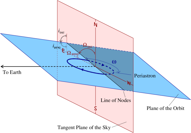
Figure 6: Geometry of the binary system, showing the position angle of ascending node in the IAU and DT92 conventions, $\Omega_{\rm IAU}$ and $\Omega_{\rm DT92}$; the inclination angle in the IAU and DT92 conventions, $i_{\rm IAU}$ and $i_{\rm DT92}$; and the angle of periastron, $\omega$, which is the same in both conventions. The cardinal directions—N, S, E and W for north, south, east, and west— are relative to whichever astrometric coordinate system is used for the pulsar position fit (equatorial or ecliptic). Red portions of the figure are in the plane of the sky; blue portions are in the orbital plane. This figure is adapted from Splaver et al. (2005).

The IAU convention has been used in Splaver et al. (2005) and NANOGrav Tempo-derived papers such as Fonseca et al. (2016) and the 12.5 yr data release (Alam et al., 2021a). The DT92 convention was used to derive the equations in Kopeikin (1995) and Kopeikin (1996) and has been used for measurements in van Straten et al. (2001) and Stairs et al. (2004). We include a diagram illustrating both conventions in Figure 6, which is adapted from Splaver et al. (2005).

The conventions used in the various pulsar timing codes are as follows:

• Tempo DDK Model (van Straten, 2003): The code used to read and write parfiles uses the IAU convention. Internally to the code, the input $i$ (“KIN”) and $\Omega$ (“KOM”) values are immediately transformed to the DT92 convention, and the Kopeikin equations are used directly in that convention. For each TOA, this code first computes the locally adjusted $x$ and $\omega$ based on equations B6 and B7, followed by the annual-orbital parallax corrections to $x$ and $\omega$ based on equations B2 and B3. It then proceeds through the standard computation of orbital delays, including Shapiro delay based on $i$, calculation of all relevant derivatives, and parameter adjustment. The fit results are transformed back to the IAU convention before ouput. Note that Tempo requires a parfile line "K96 1" to ensure that the proper-motion corrections are done.

• Tempo2 DDK model: The code used to read and write parfiles uses the DT92 convention for KIN and KOM. The delay/derivative code closely follows the logic of the Tempo DDK code, including the use of the DT92 convention in the Kopeikin equations. We have recently debugged this routine and confirmed that it returns equivalent results to the tempo DDK model.

• Tempo2 T2 model: The code used to read and write parfiles uses the IAU convention for KIN and KOM. This model provides a superset of multiple binary models, and uses equation B1 directly rather than breaking it down. The fitting code uses an IAU-convention implementation of the Kopeikin equations. We note that only the base values of $i$, $x$ and $\omega$, not values adjusted via equations B5 –B7, are used in determining the annual-orbital parallax terms and also the Romer delay. This introduces small discrepancies between its results and those of DDK, with the T2 model parameters being incorrect by up to roughly 0.2 sigma, according to our simulations.

• PINT DDK model: The code used to read and write parfiles uses the DT92 convention for KIN and KOM. Internally the code uses the equations from Kopeikin (1995) and Kopeikin (1996) directly. The PINT code does apply corrections based on equations B5 –B7 before computing the annual-orbital parallax terms.

In this paper, we present astrometric results in ecliptic coordinates rather than equatorial. Tempo and PINT are written to fit for $\Omega$ relative to ecliptic North (Tempo) or East (PINT) rather than equatorial North/East in this case, and use the proper motions in ecliptic coordinates ($\mu_{\lambda},\mu_{\beta}$) to calculate the relevant parameters.

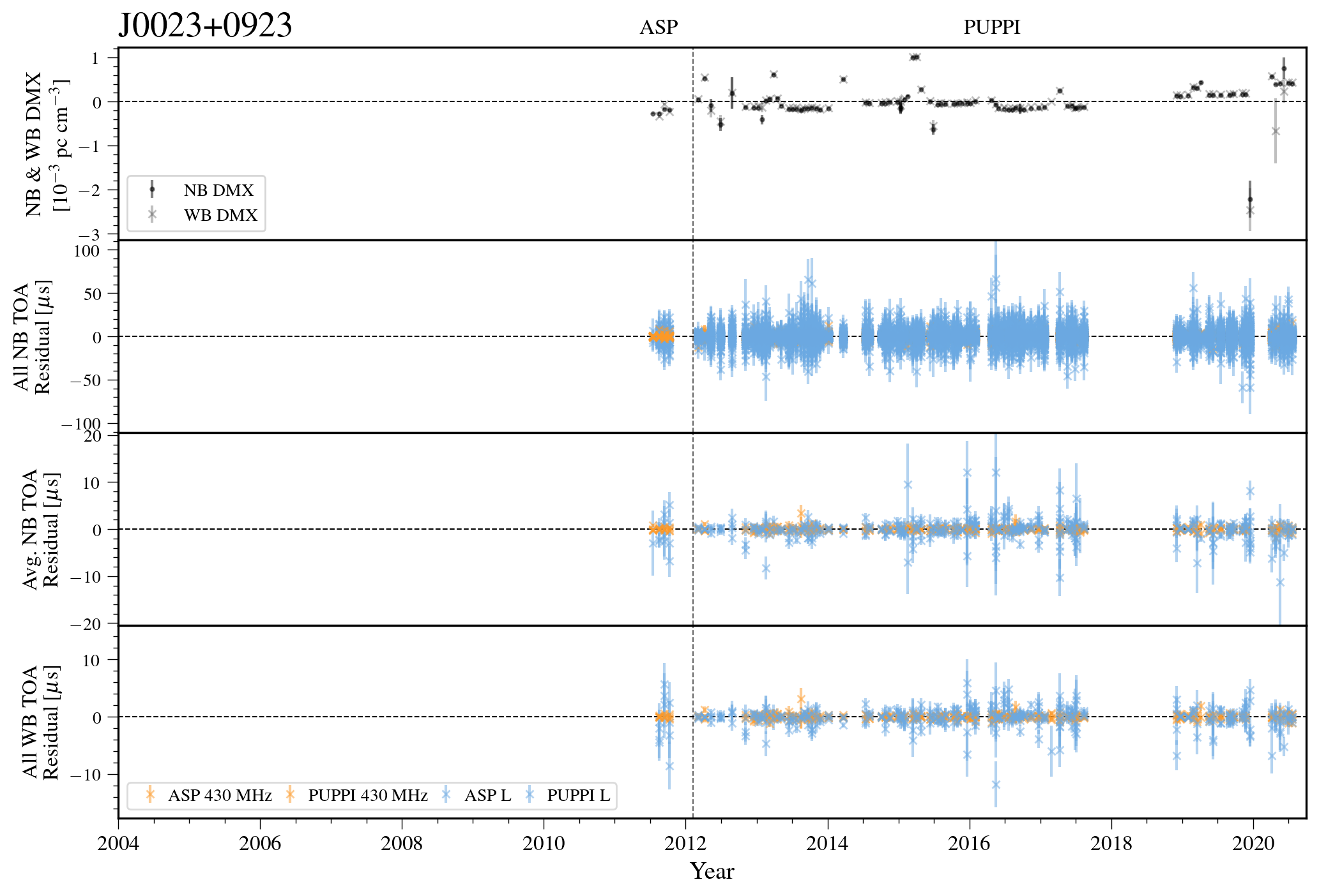
Figure 7: Narrowband and wideband timing residuals and DMX timeseries for J0023+0923. The wideband data set (and therefore, the wideband residuals and DMX timeseries presented here) are only used for pipeline development and the mass determinations presented in Section 5.1.3. Panel 1: Narrowband and wideband DMX variations. Panel 2: Residual arrival times for all TOAs. Points are semi-transparent; dark regions arise from the overlap of many points. Panel 3: Average residual arrival times. Panel 4 (in 4-panel plots): All wideband TOA residuals. Receivers and backends corresponding to each TOA are shown in the bottom panel’s legend. Dashed vertical line(s) denote the divide between backend systems.

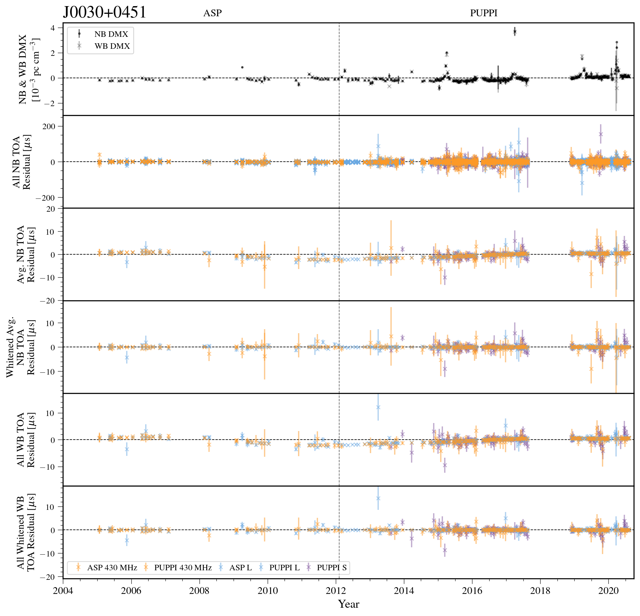
Figure 8: Narrowband and wideband timing residuals and DMX timeseries for J0030+0451. The wideband data set (and therefore, the wideband residuals and DMX timeseries presented here) are only used for pipeline development and the mass determinations presented in Section 5.1.3. Panel 1: Narrowband and wideband DMX variations. Panel 2: Residual arrival times for all TOAs. Points are semi-transparent; dark regions arise from the overlap of many points. Panel 3: Average residual arrival times. Panel 4 (in 6-panel plots): Whitened average narrowband TOA residuals. Panel 5: All wideband TOA residuals. Panel 6: All whitened wideband TOA residuals. Receivers and backends corresponding to each TOA are shown in the bottom panel’s legend. Dashed vertical line(s) denote the divide between backend systems.

Figure 9: Narrowband and wideband timing residuals and DMX timeseries for J0340+4130. See Figure 7 for details.

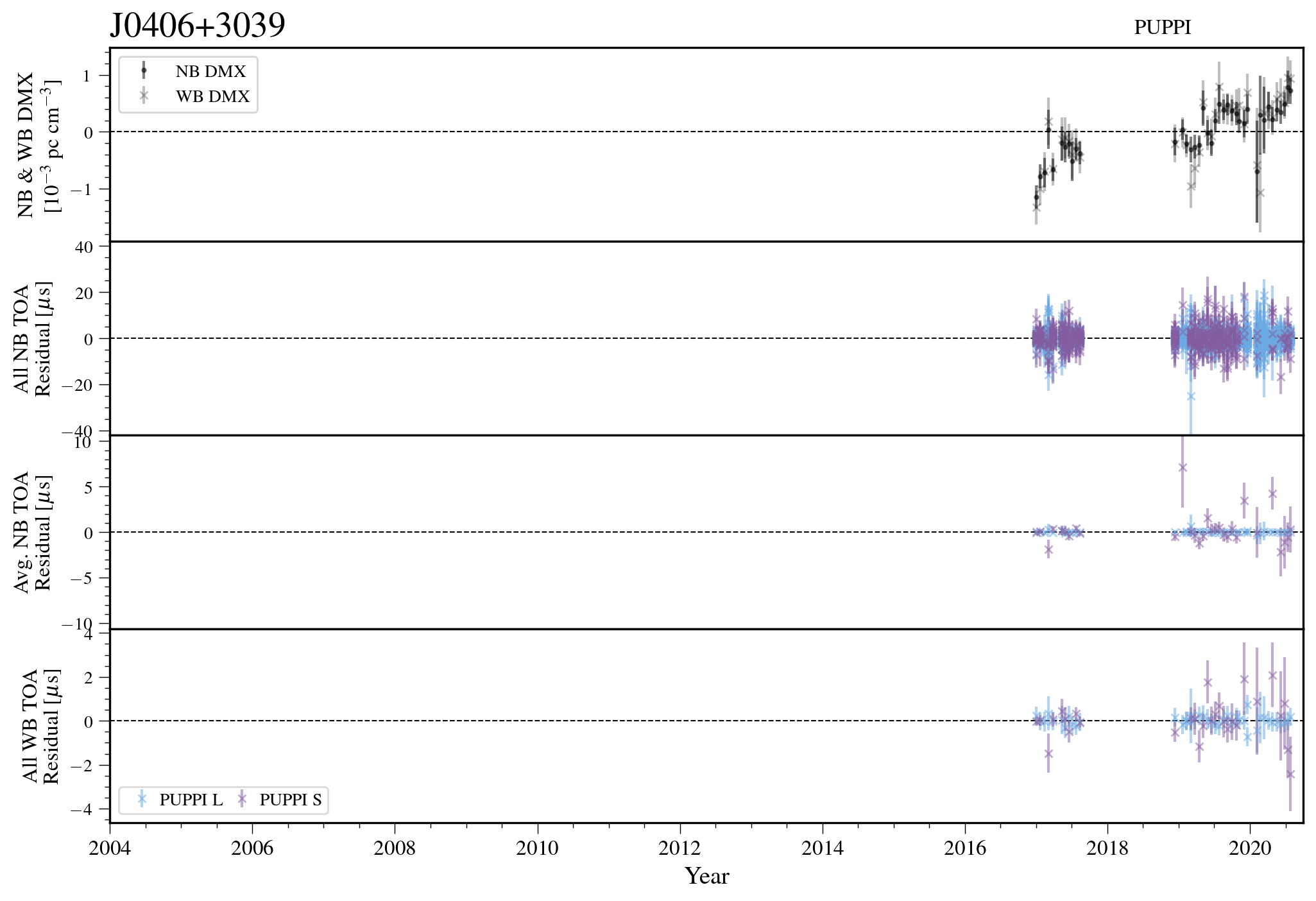
Figure 10: Narrowband and wideband timing residuals and DMX timeseries for J0406+3039. See Figure 7 for details.

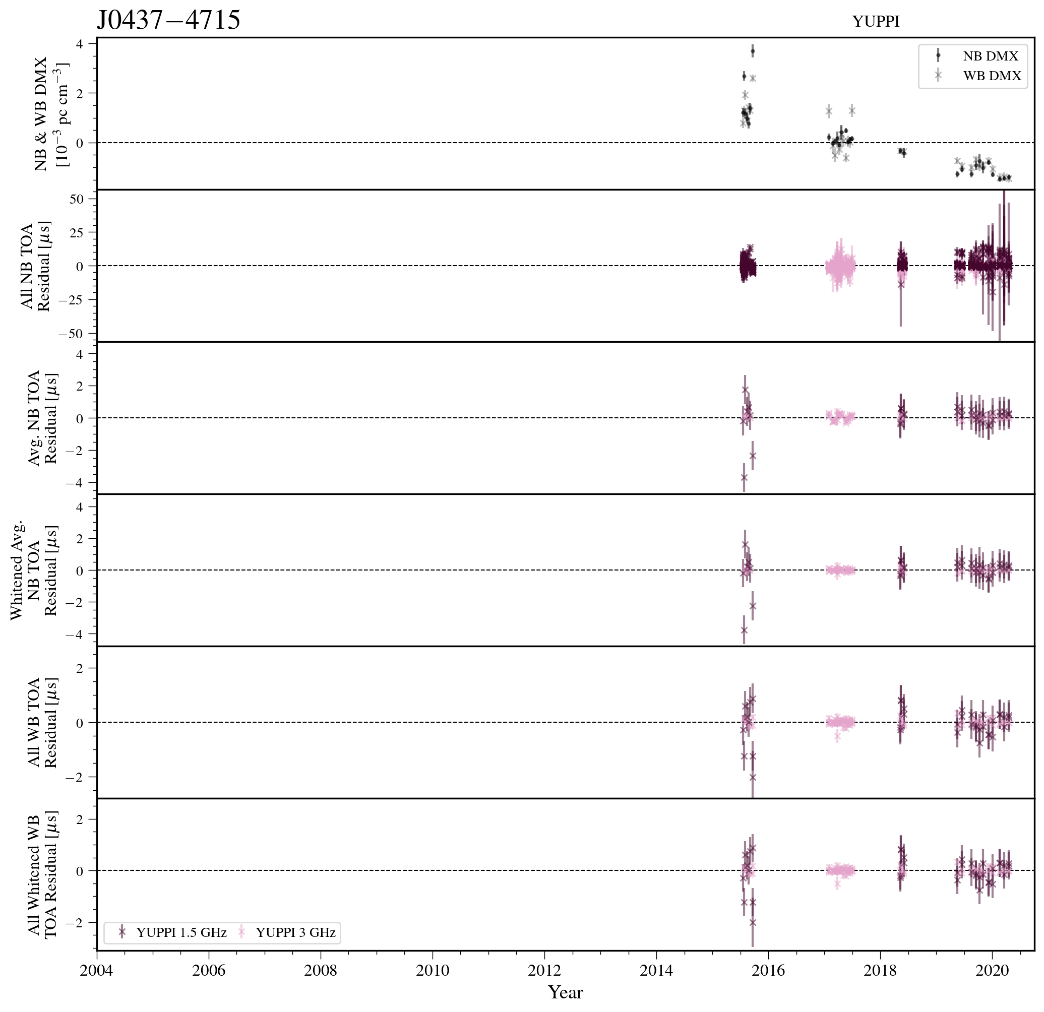
Figure 11: Narrowband and wideband timing residuals and DMX timeseries for J0437-4715. See Figure 8 for details.

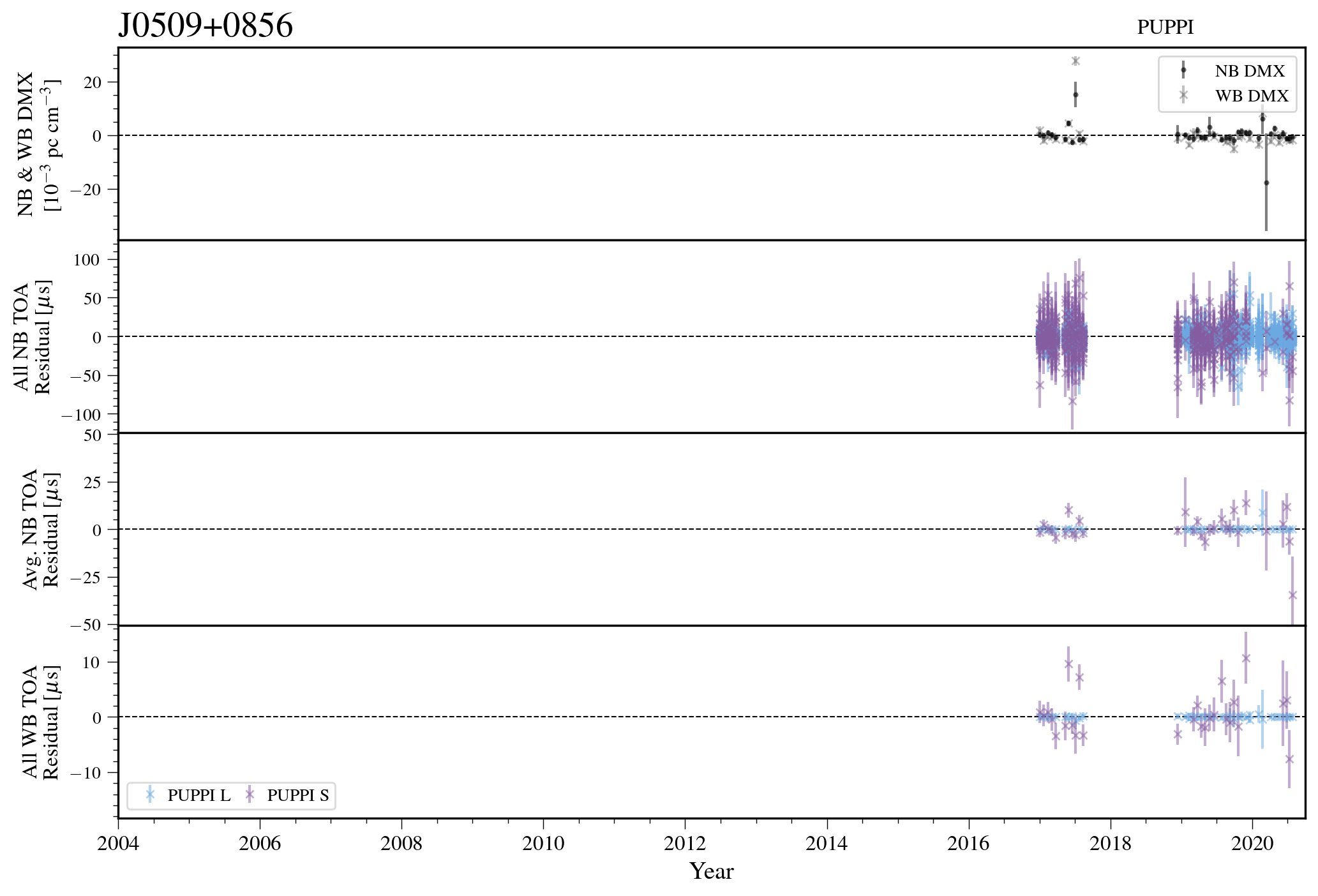
Figure 12: Narrowband and wideband timing residuals and DMX timeseries for J0509+0856. See Figure 7 for details.

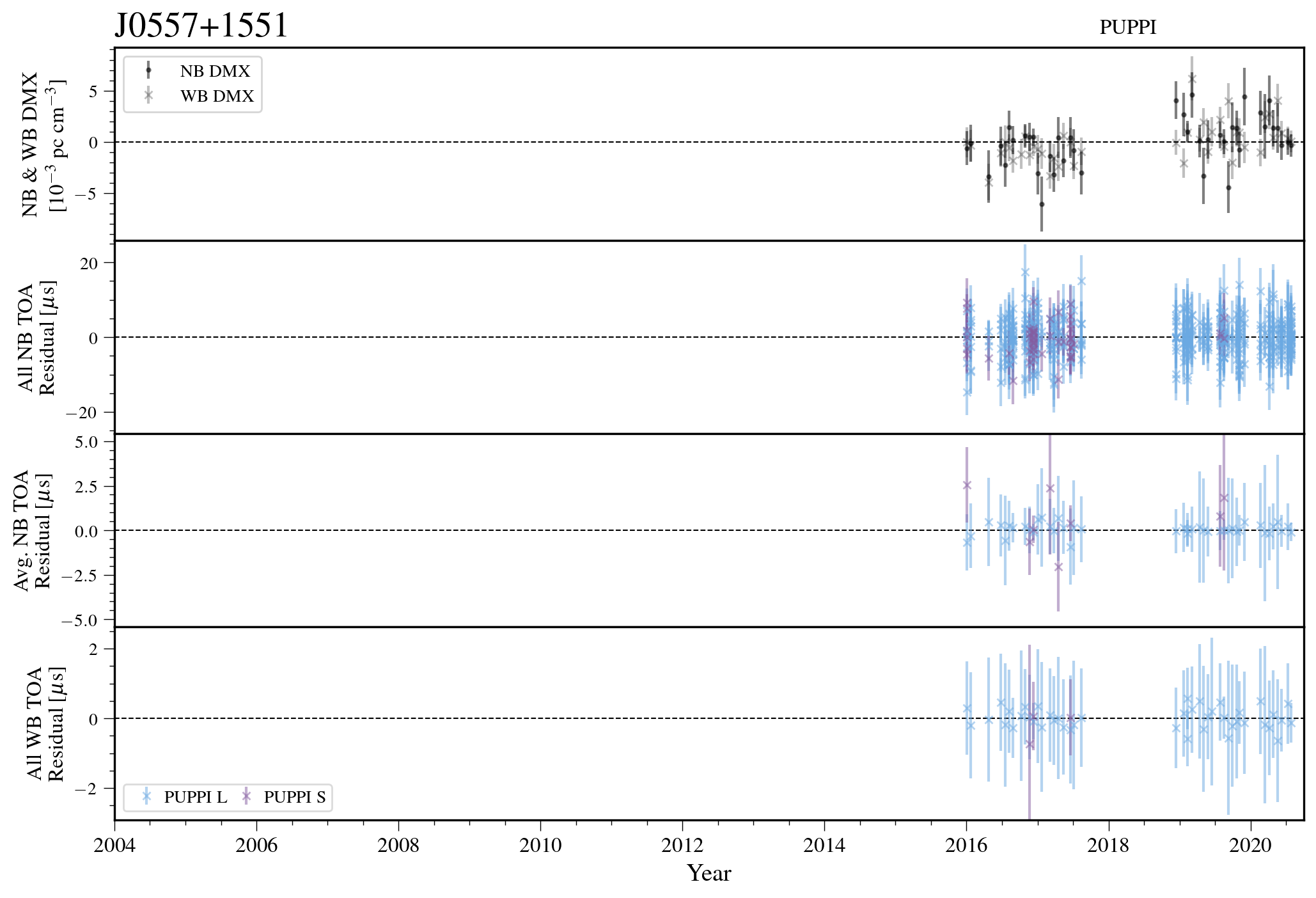
Figure 13: Narrowband and wideband timing residuals and DMX timeseries for J0557+1551. See Figure 7 for details.

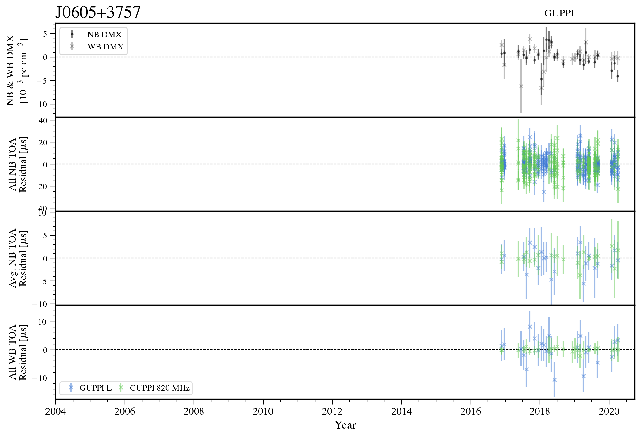
Figure 14: Narrowband and wideband timing residuals and DMX timeseries for J0605+3757. See Figure 7 for details.

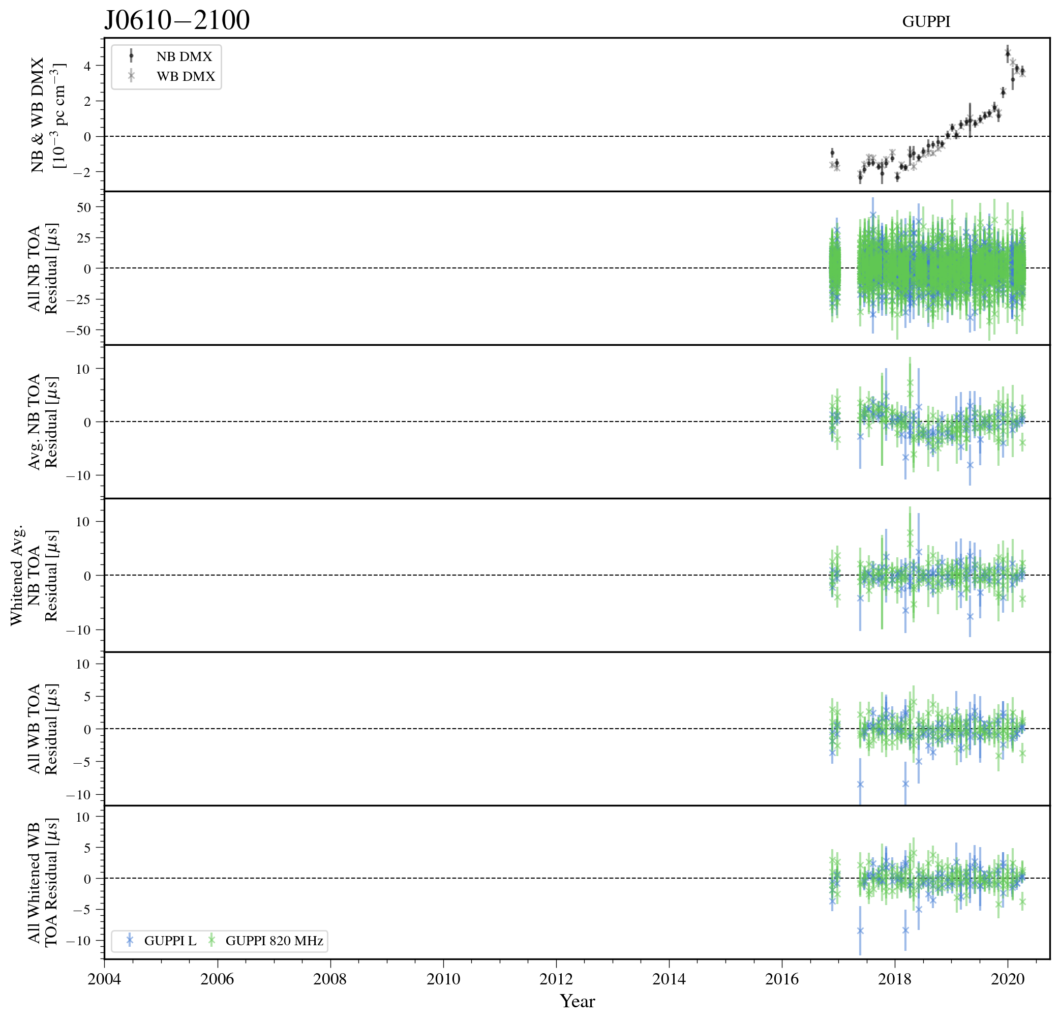
Figure 15: Narrowband and wideband timing residuals and DMX timeseries for J0610-2100. See Figure 8 for details.

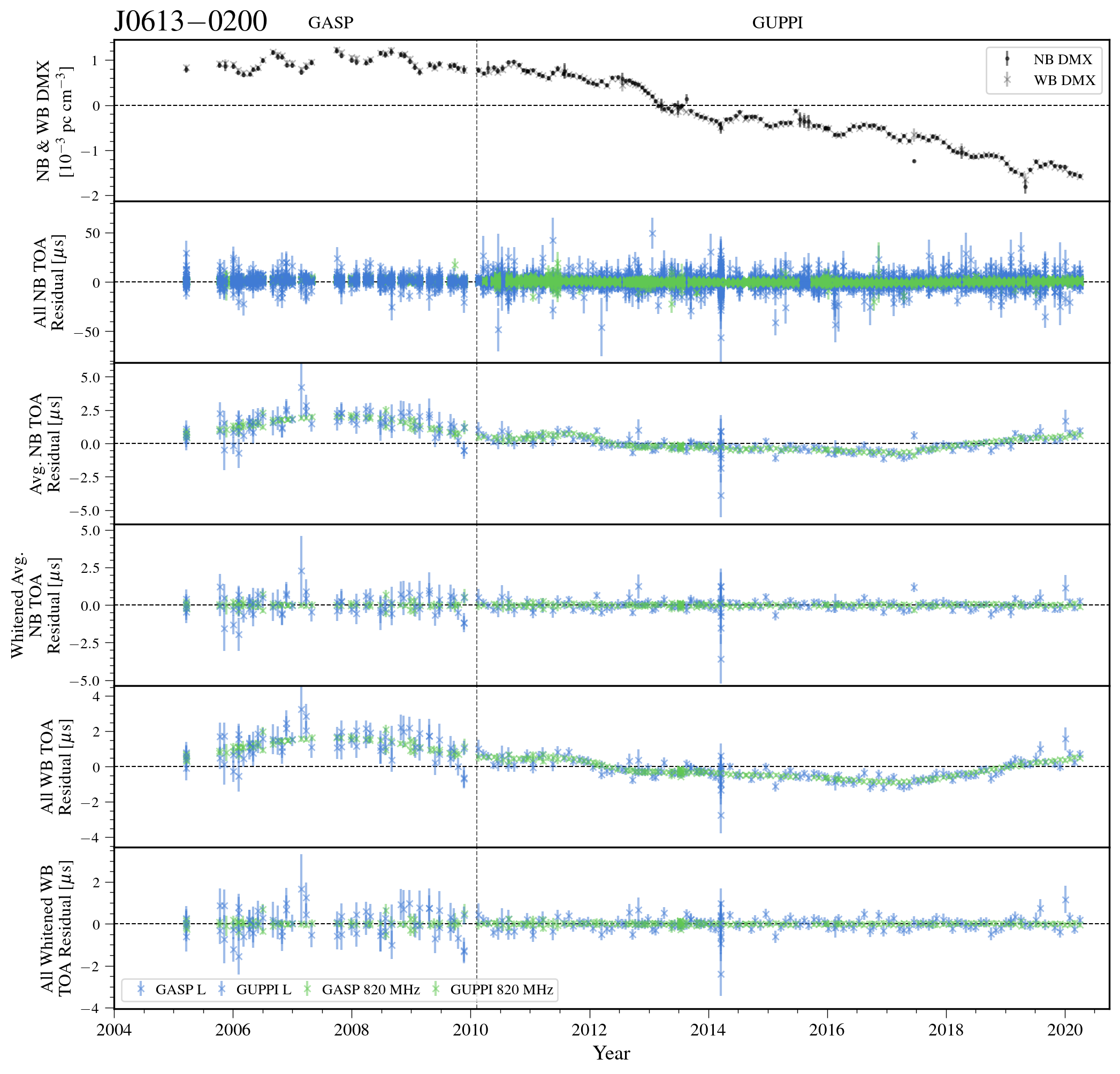
Figure 16: Narrowband and wideband timing residuals and DMX timeseries for J0613-0200. See Figure 8 for details.

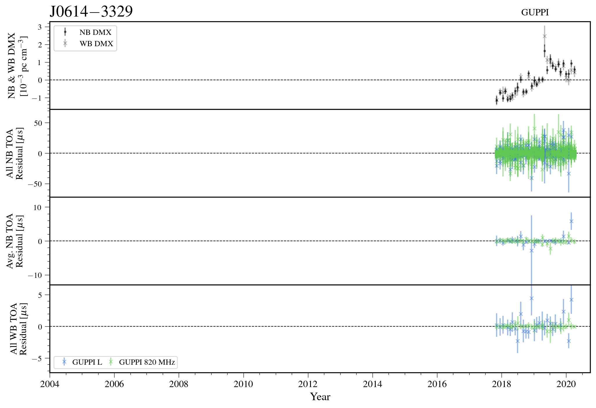
Figure 17: Narrowband and wideband timing residuals and DMX timeseries for J0614-3329. See Figure 7 for details.

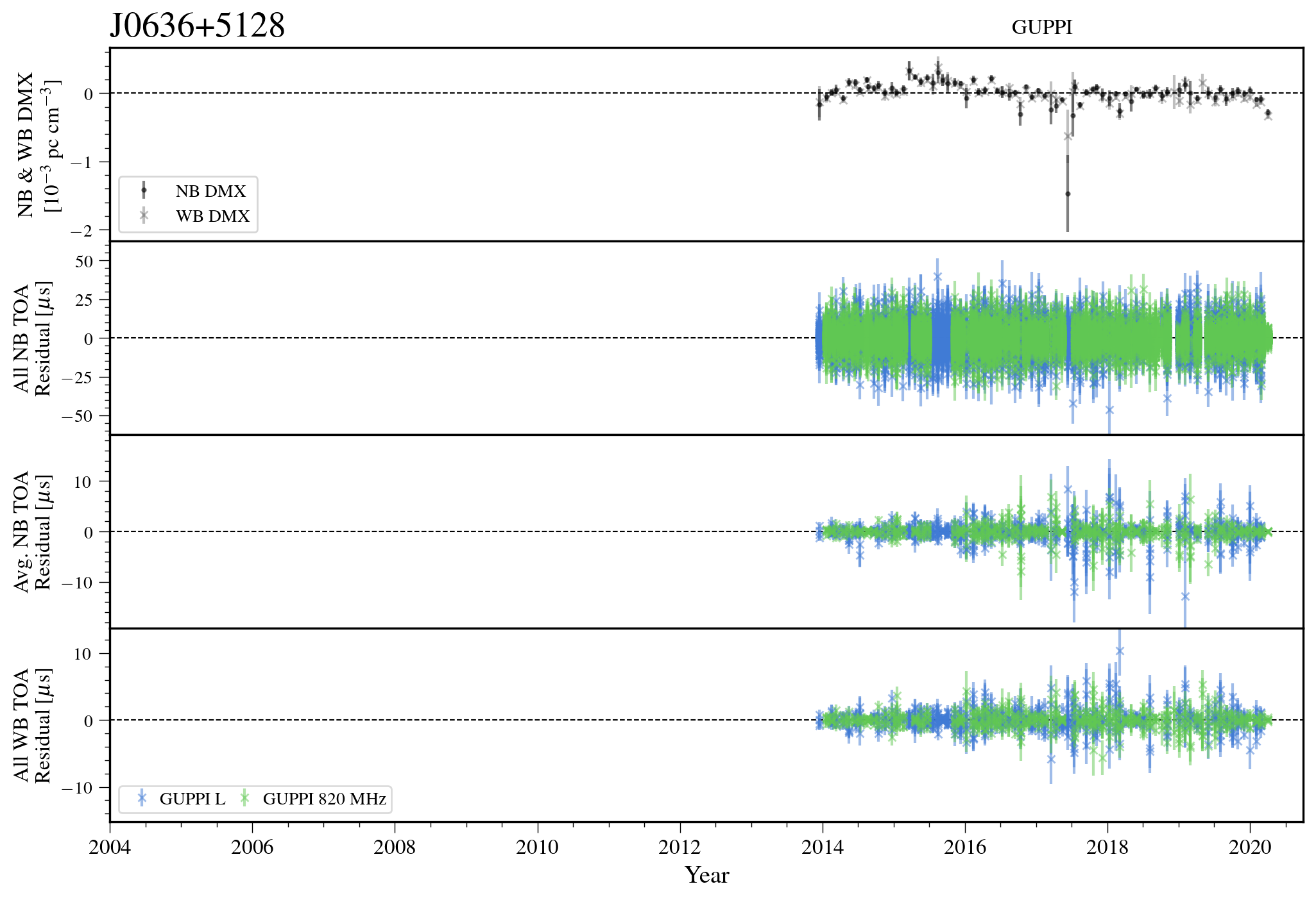
Figure 18: Narrowband and wideband timing residuals and DMX timeseries for J0636+5128. See Figure 7 for details.

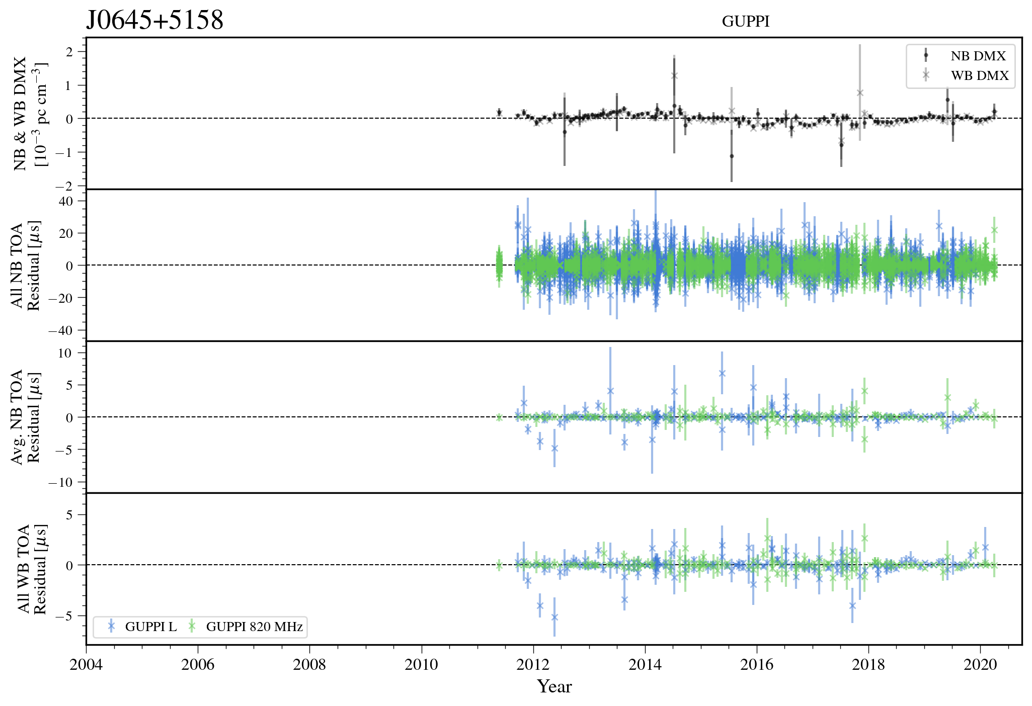
Figure 19: Narrowband and wideband timing residuals and DMX timeseries for J0645+5158. See Figure 7 for details.

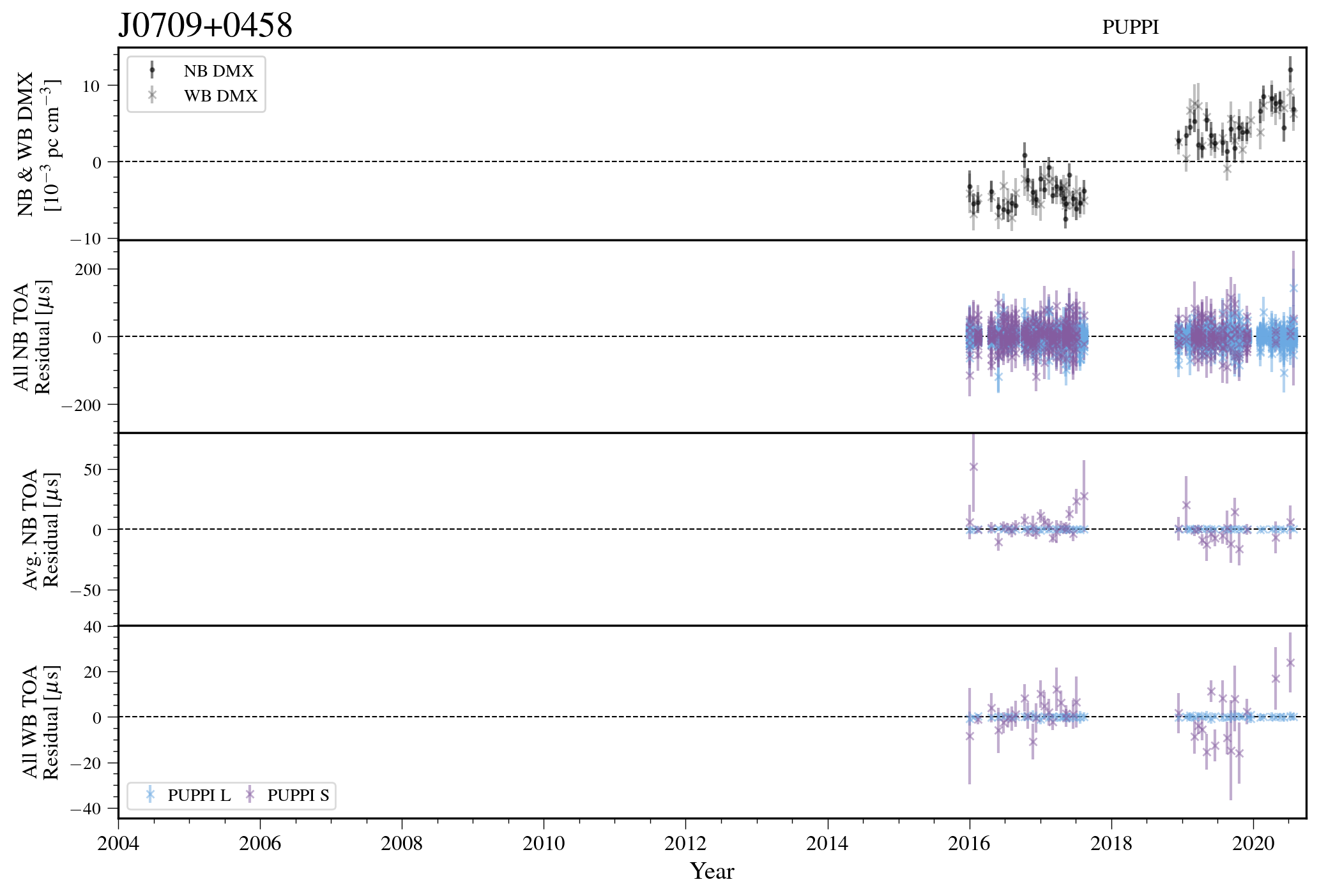
Figure 20: Narrowband and wideband timing residuals and DMX timeseries for J0709+0458. See Figure 7 for details.

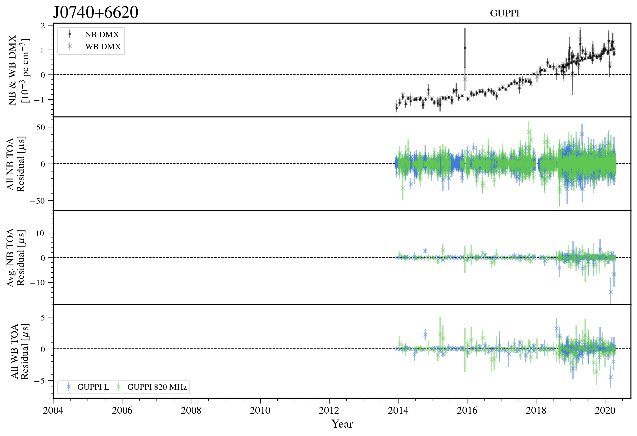
Figure 21: Narrowband and wideband timing residuals and DMX timeseries for J0740+6620. See Figure 7 for details.

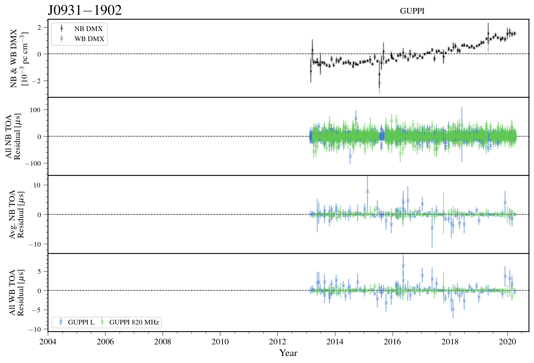
Figure 22: Narrowband and wideband timing residuals and DMX timeseries for J0931-1902. See Figure 7 for details.

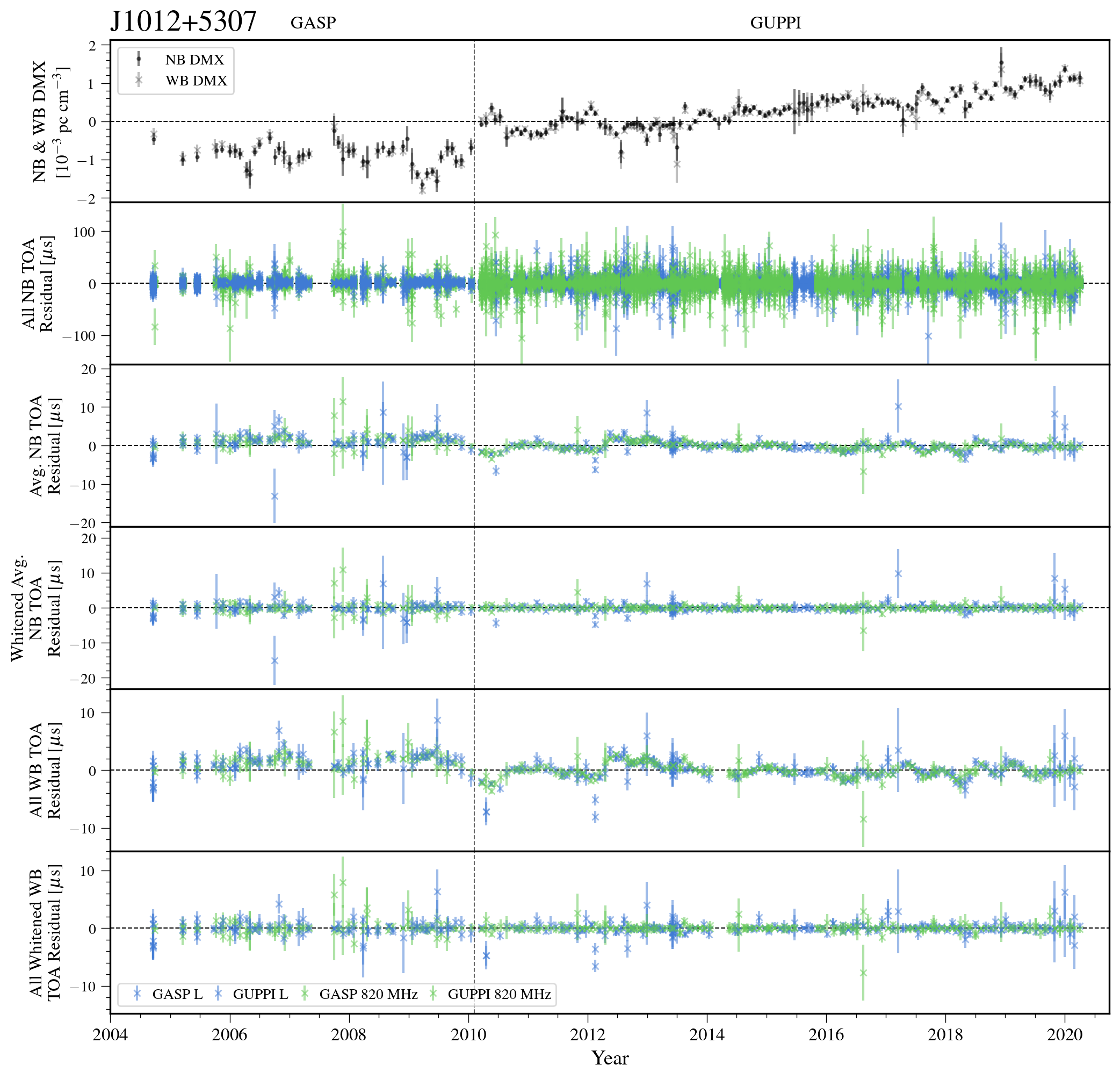
Figure 23: Narrowband and wideband timing residuals and DMX timeseries for J1012+5307. See Figure 8 for details.

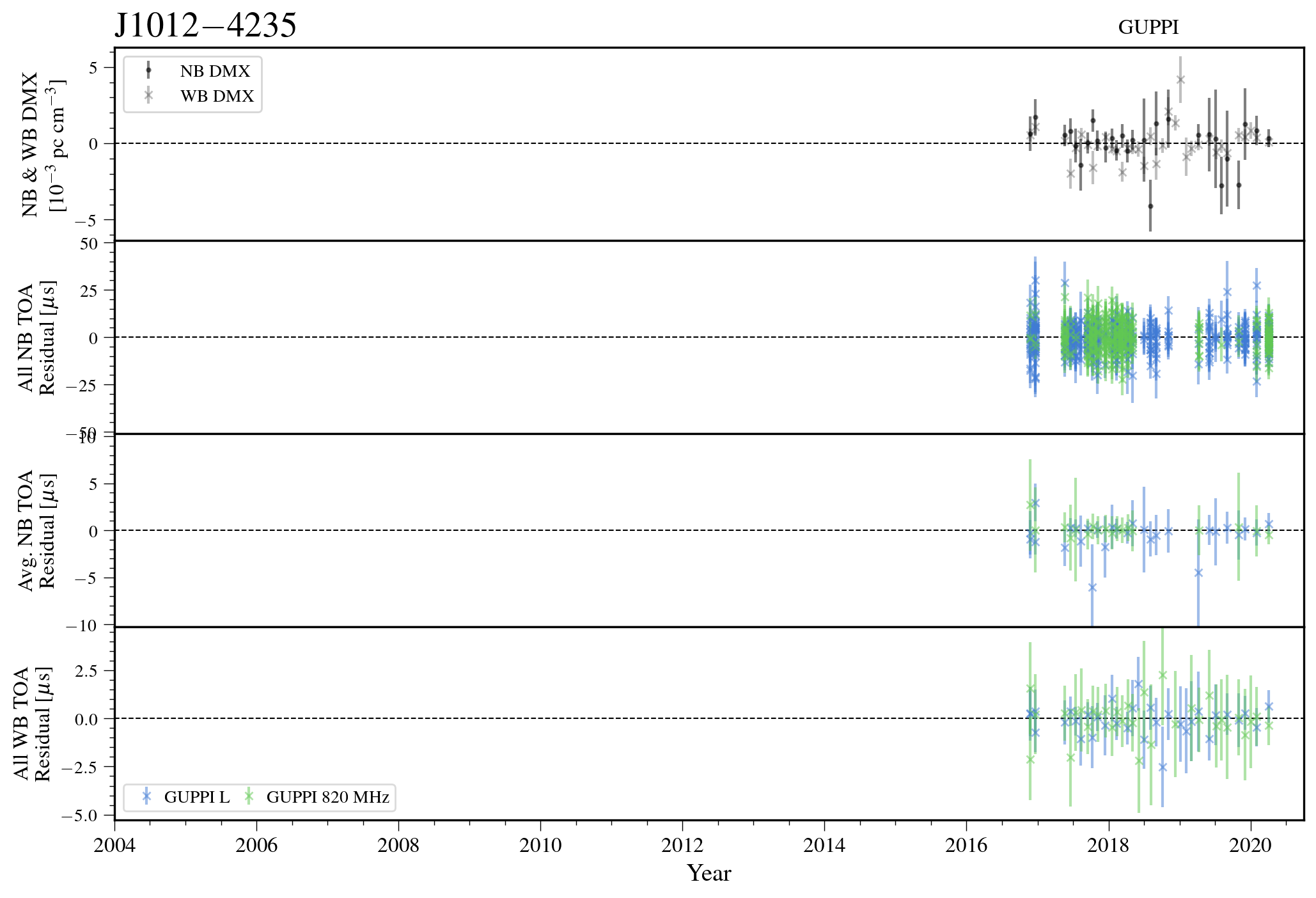
Figure 24: Narrowband and wideband timing residuals and DMX timeseries for J1012-4235. See Figure 7 for details.

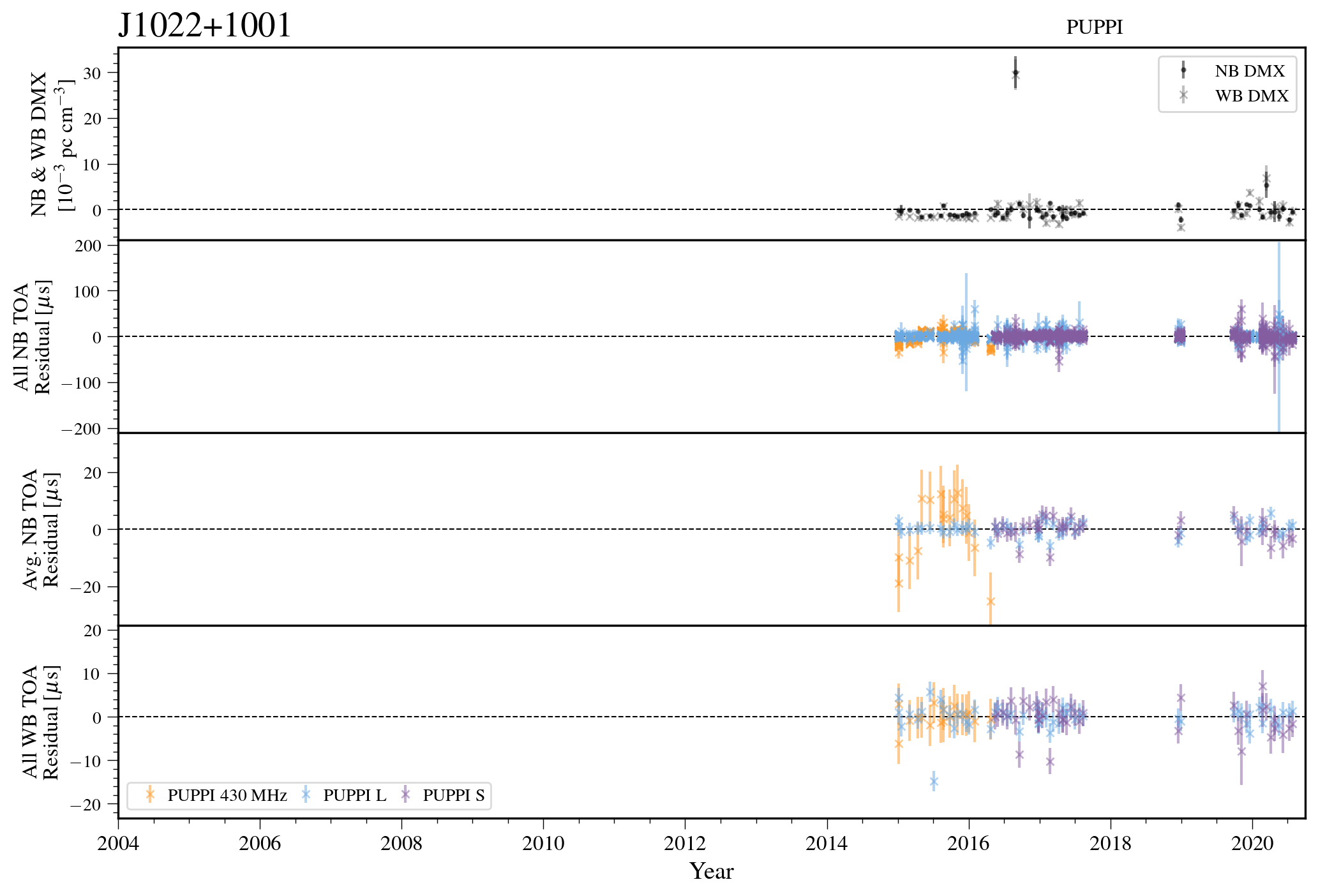
Figure 25: Narrowband and wideband timing residuals and DMX timeseries for J1022+1001. See Figure 7 for details.

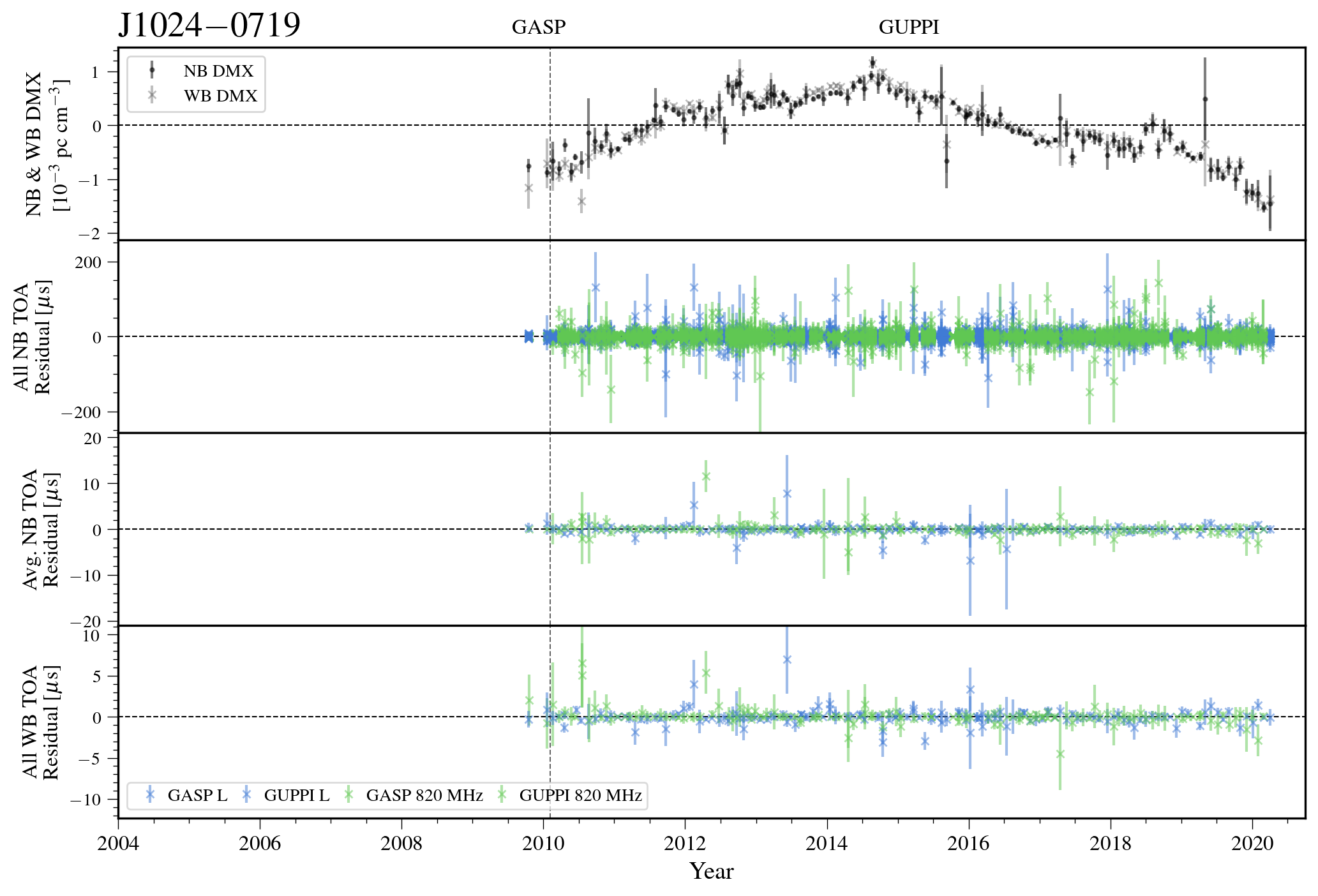
Figure 26: Narrowband and wideband timing residuals and DMX timeseries for J1024-0719. See Figure 7 for details.

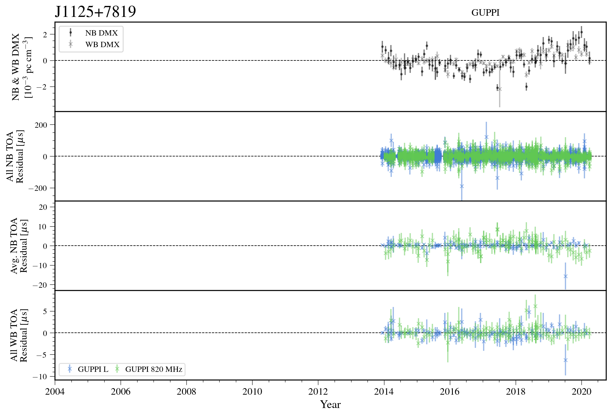
Figure 27: Narrowband and wideband timing residuals and DMX timeseries for J1125+7819. See Figure 7 for details.

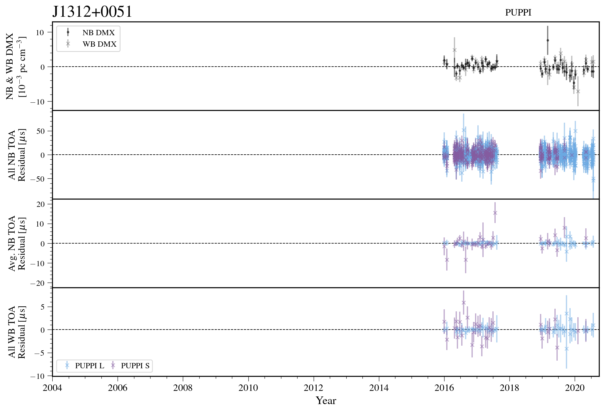
Figure 28: Narrowband and wideband timing residuals and DMX timeseries for J1312+0051. See Figure 7 for details.

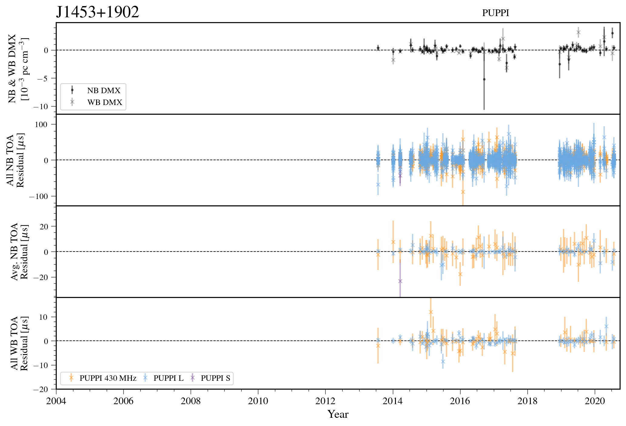
Figure 29: Narrowband and wideband timing residuals and DMX timeseries for J1453+1902. See Figure 7 for details.

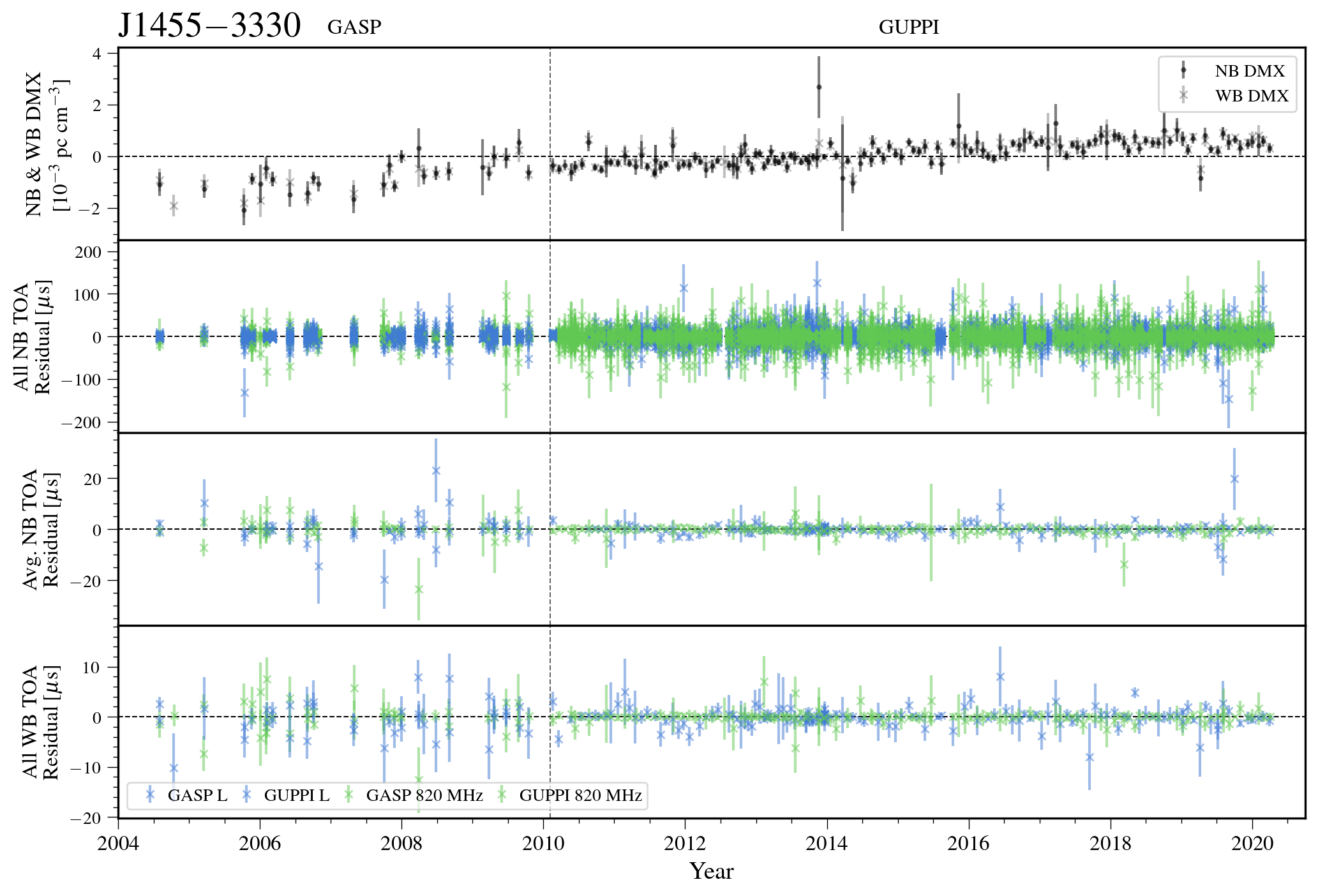
Figure 30: Narrowband and wideband timing residuals and DMX timeseries for J1455-3330. See Figure 7 for details.

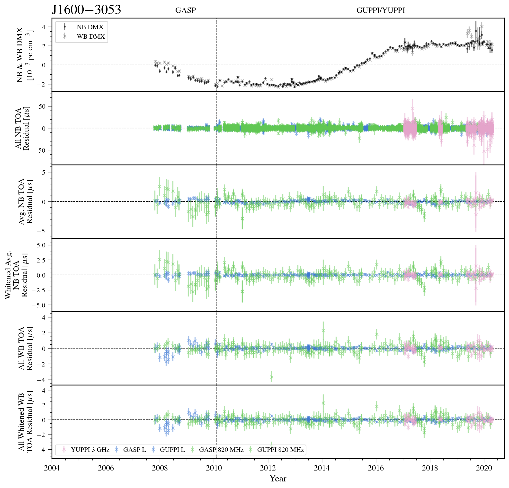
Figure 31: Narrowband and wideband timing residuals and DMX timeseries for J1600-3053. See Figure 8 for details.

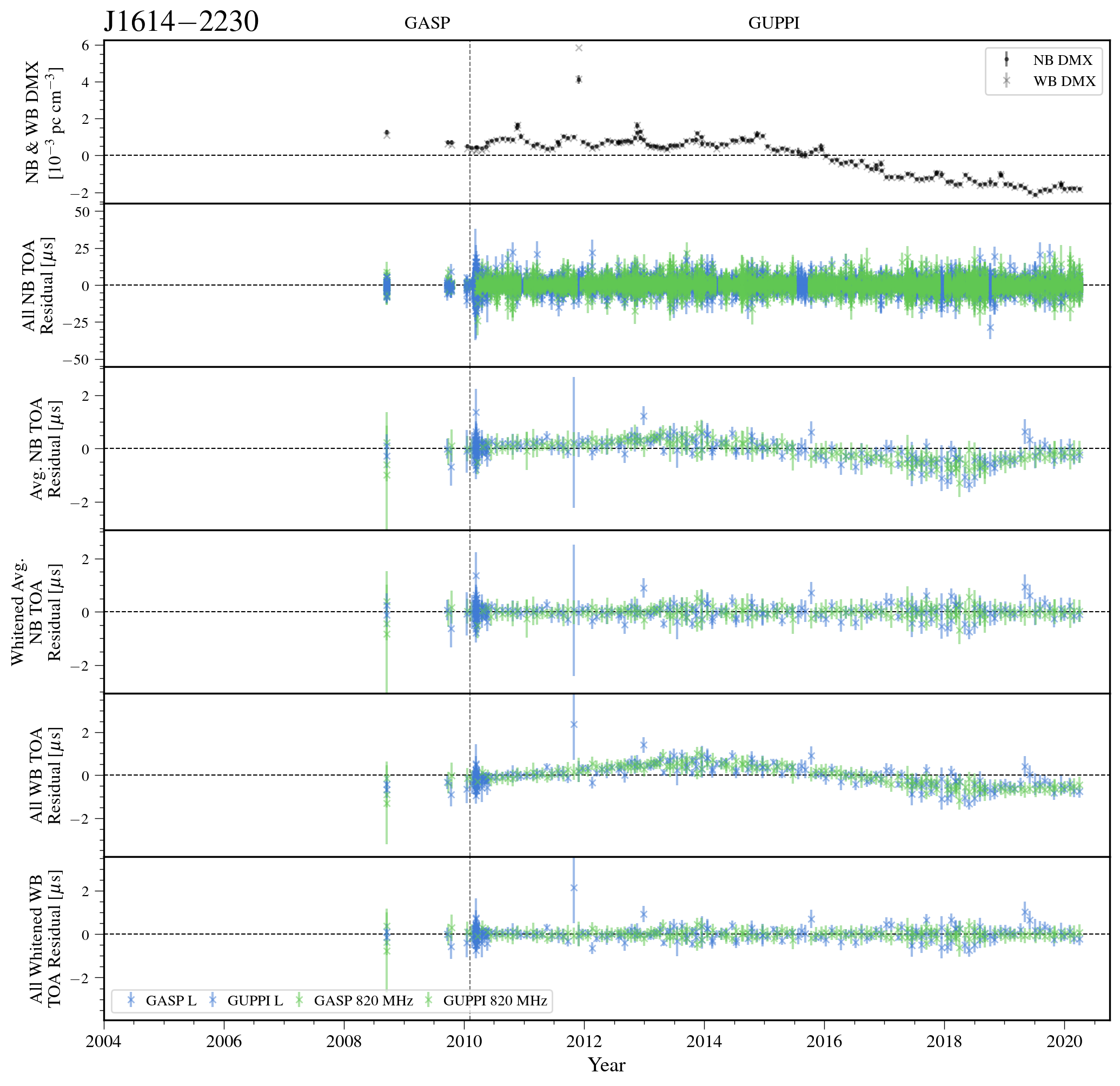
Figure 32: Narrowband and wideband timing residuals and DMX timeseries for J1614-2230. See Figure 8 for details.

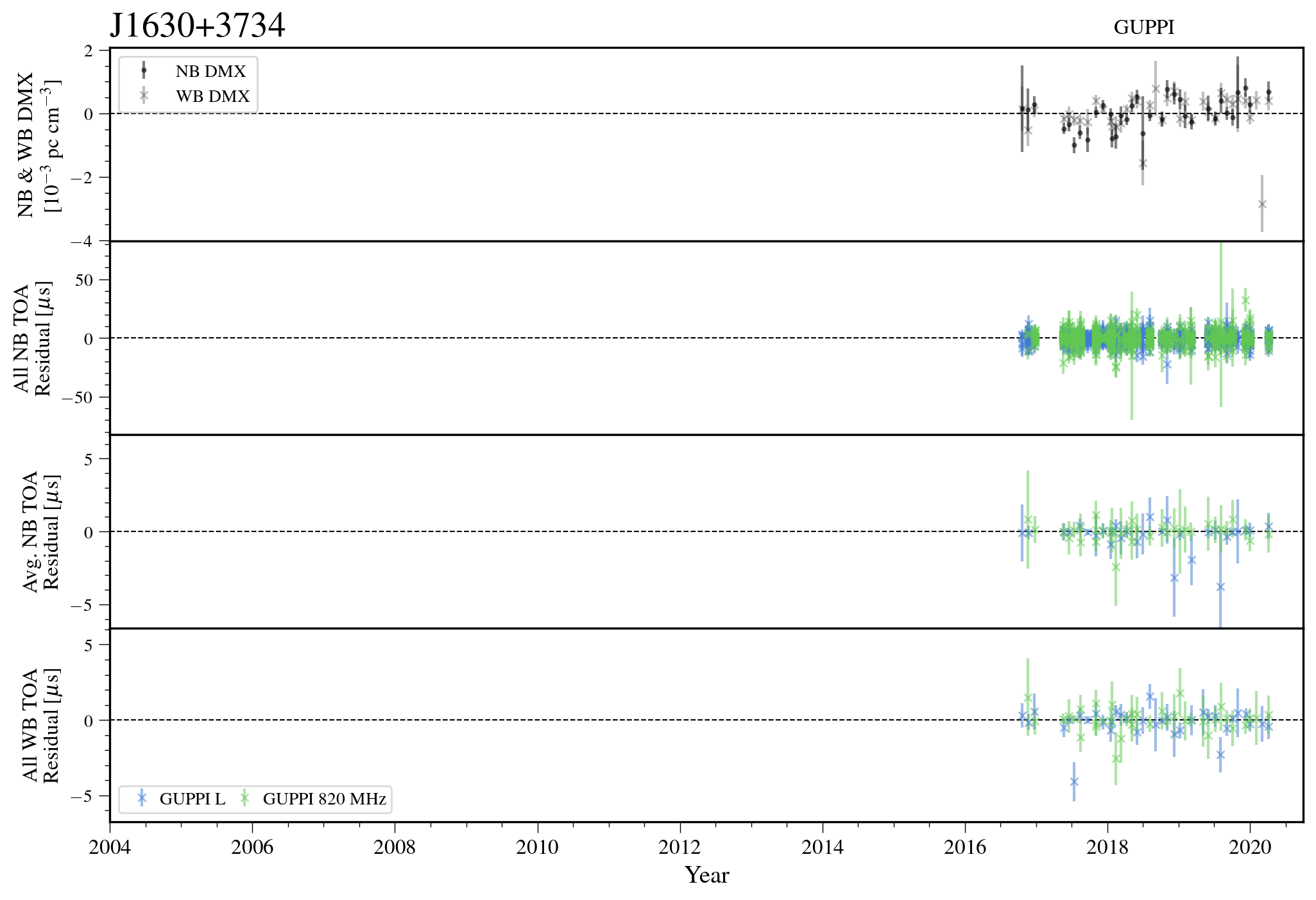
Figure 33: Narrowband and wideband timing residuals and DMX timeseries for J1630+3734. See Figure 7 for details.

Figure 34: Narrowband and wideband timing residuals and DMX timeseries for J1640+2224. See Figure 7 for details.

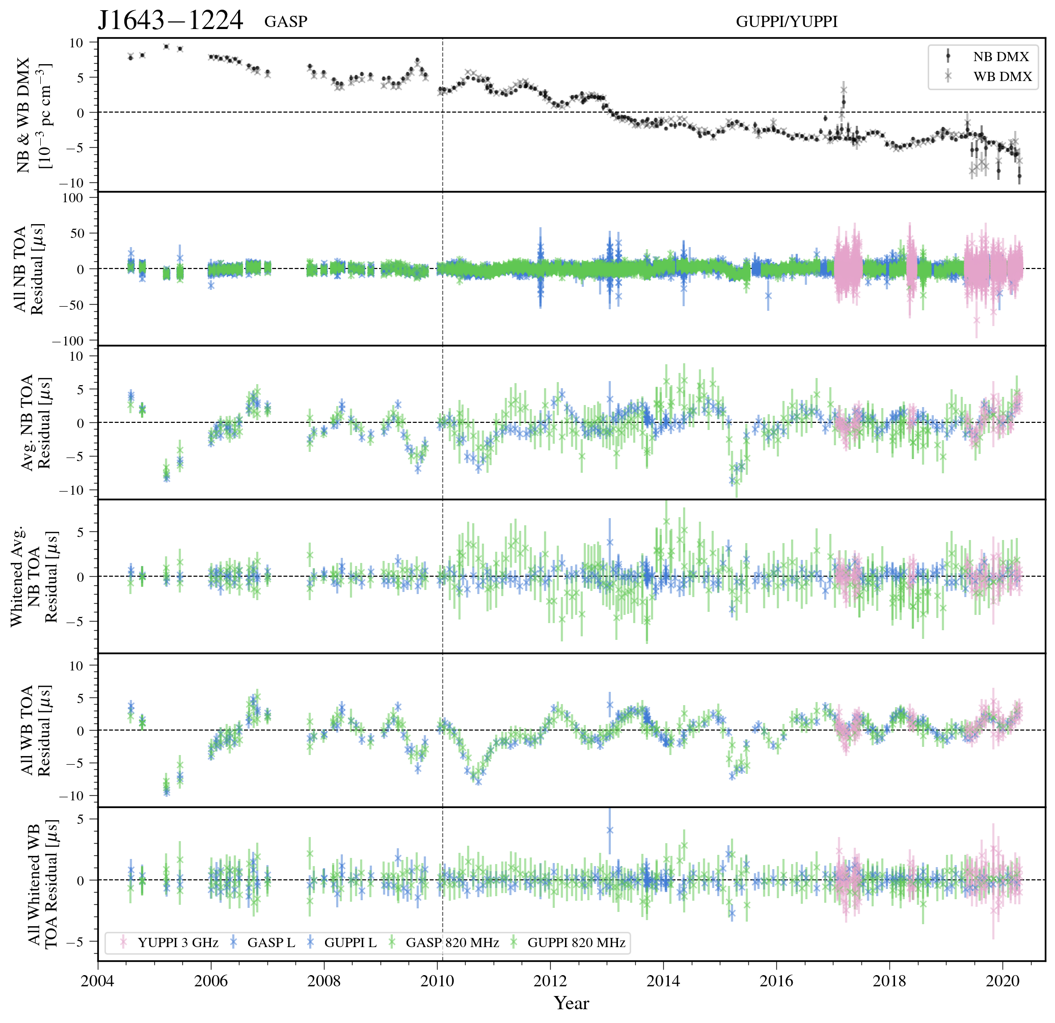
Figure 35: Narrowband and wideband timing residuals and DMX timeseries for J1643-1224. See Figure 8 for details.

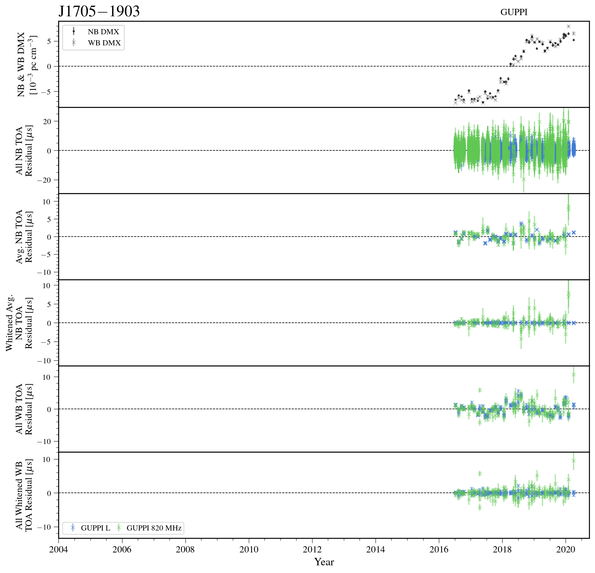
Figure 36: Narrowband and wideband timing residuals and DMX timeseries for J1705-1903. See Figure 8 for details.

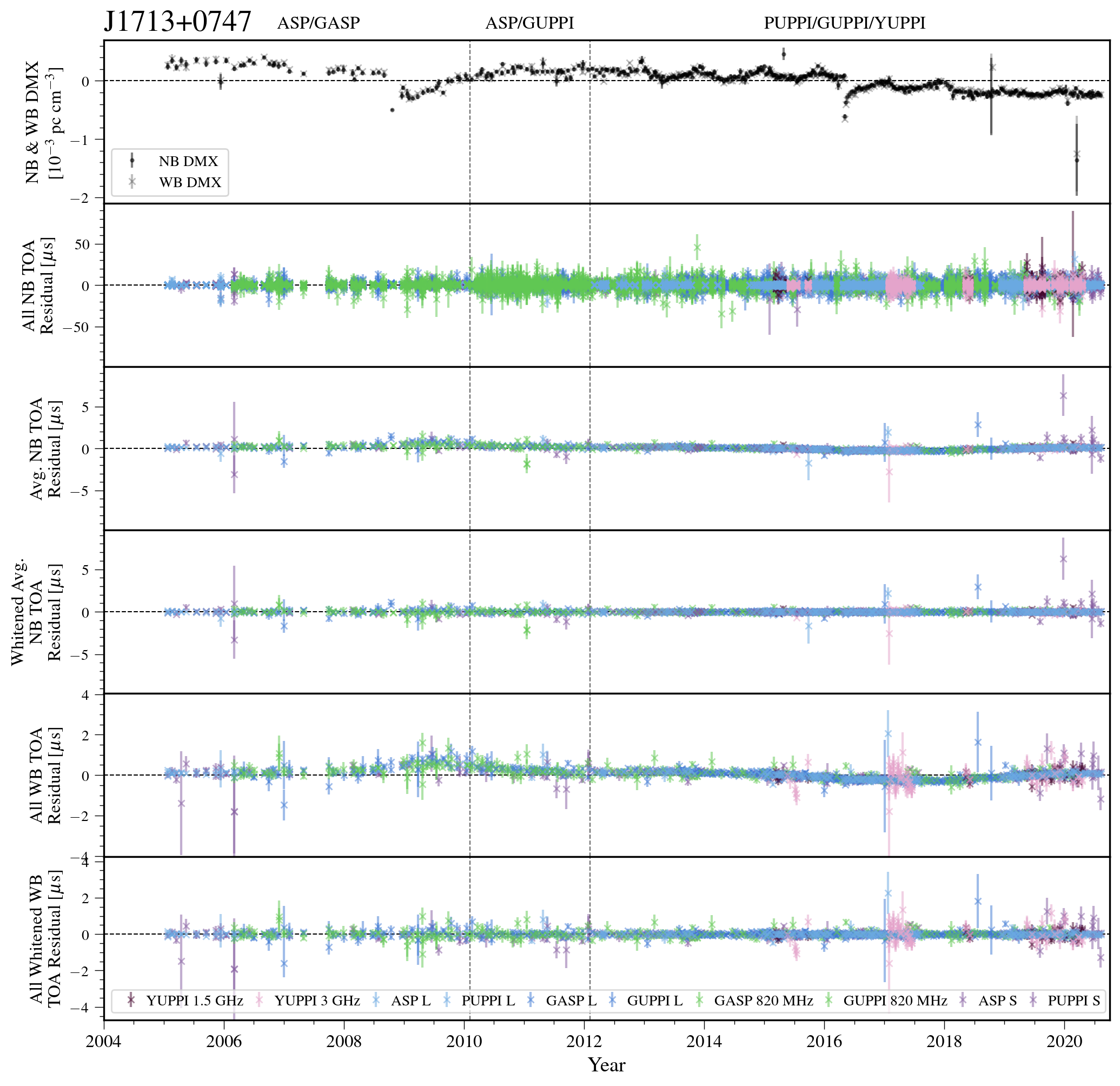
Figure 37: Narrowband and wideband timing residuals and DMX timeseries for J1713+0747. See Figure 8 for details.

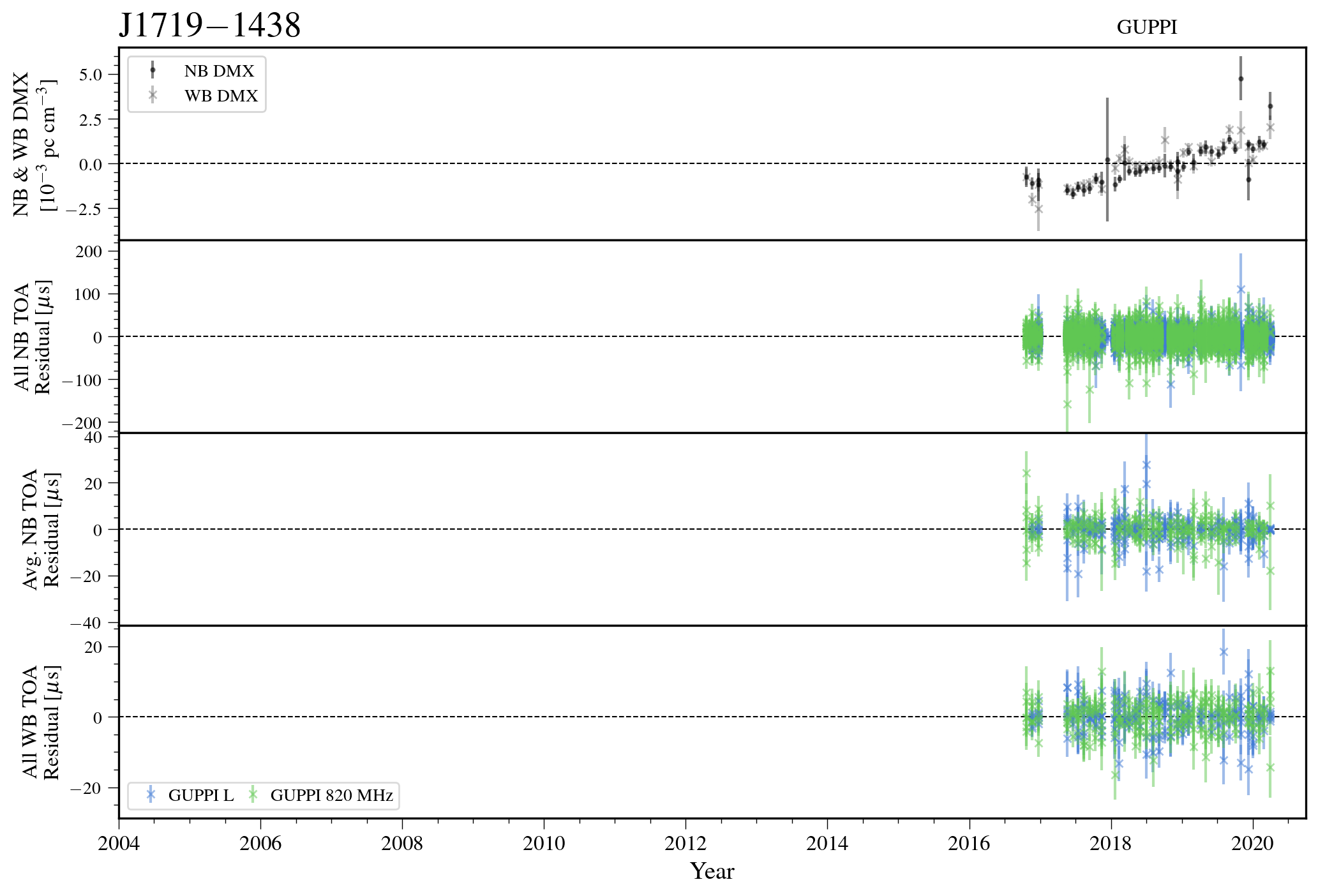
Figure 38: Narrowband and wideband timing residuals and DMX timeseries for J1719-1438. See Figure 7 for details.

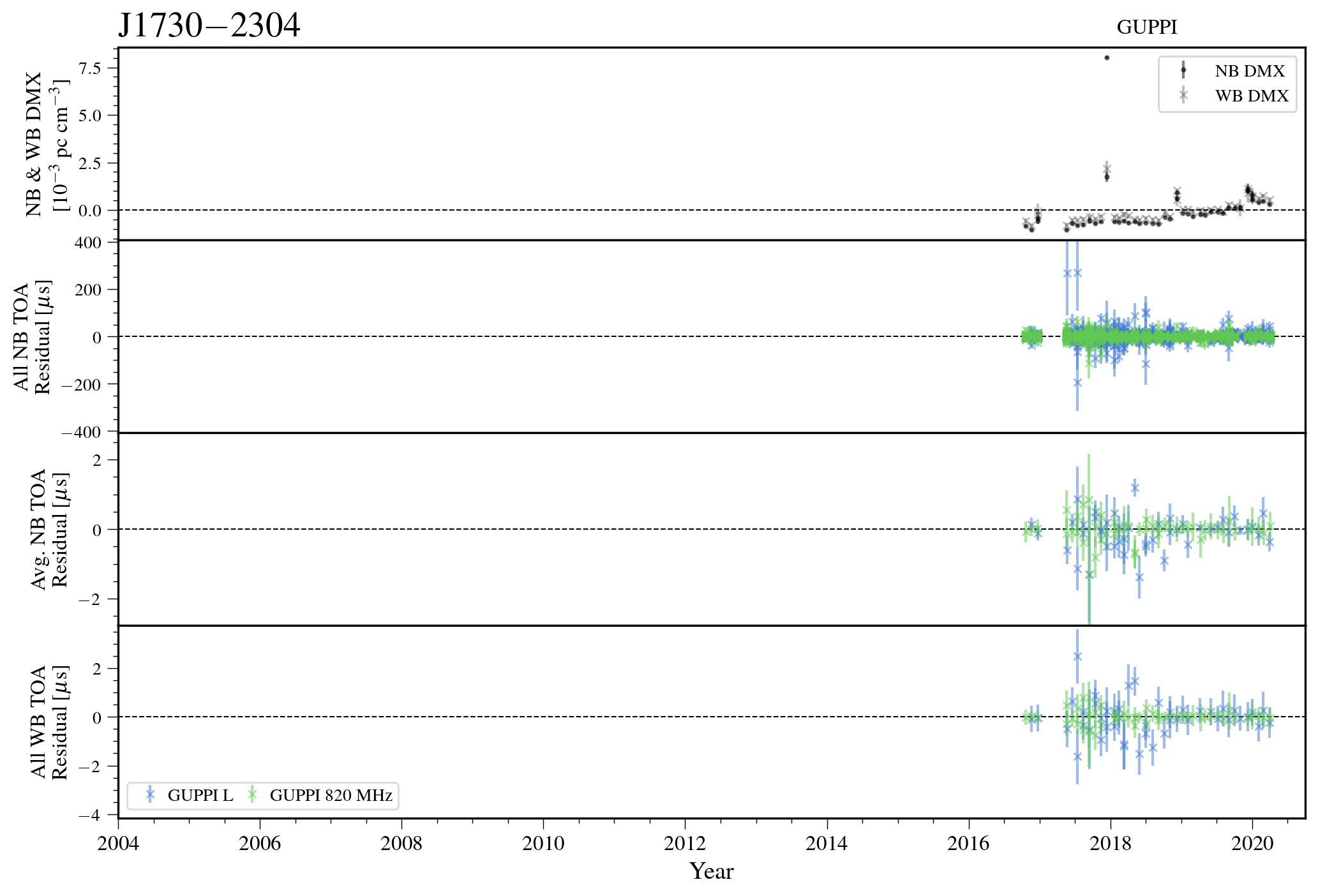
Figure 39: Narrowband and wideband timing residuals and DMX timeseries for J1730-2304. See Figure 7 for details.

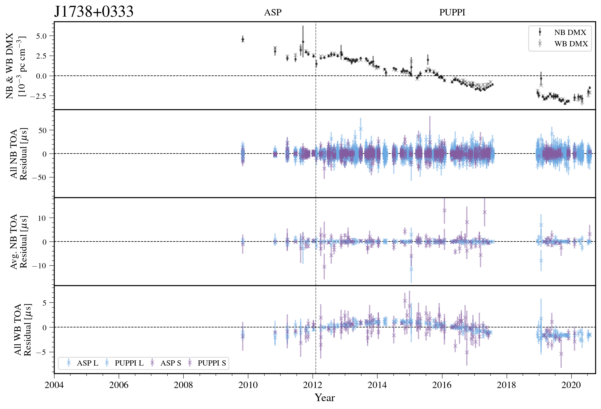
Figure 40: Narrowband and wideband timing residuals and DMX timeseries for J1738+0333. See Figure 7 for details.

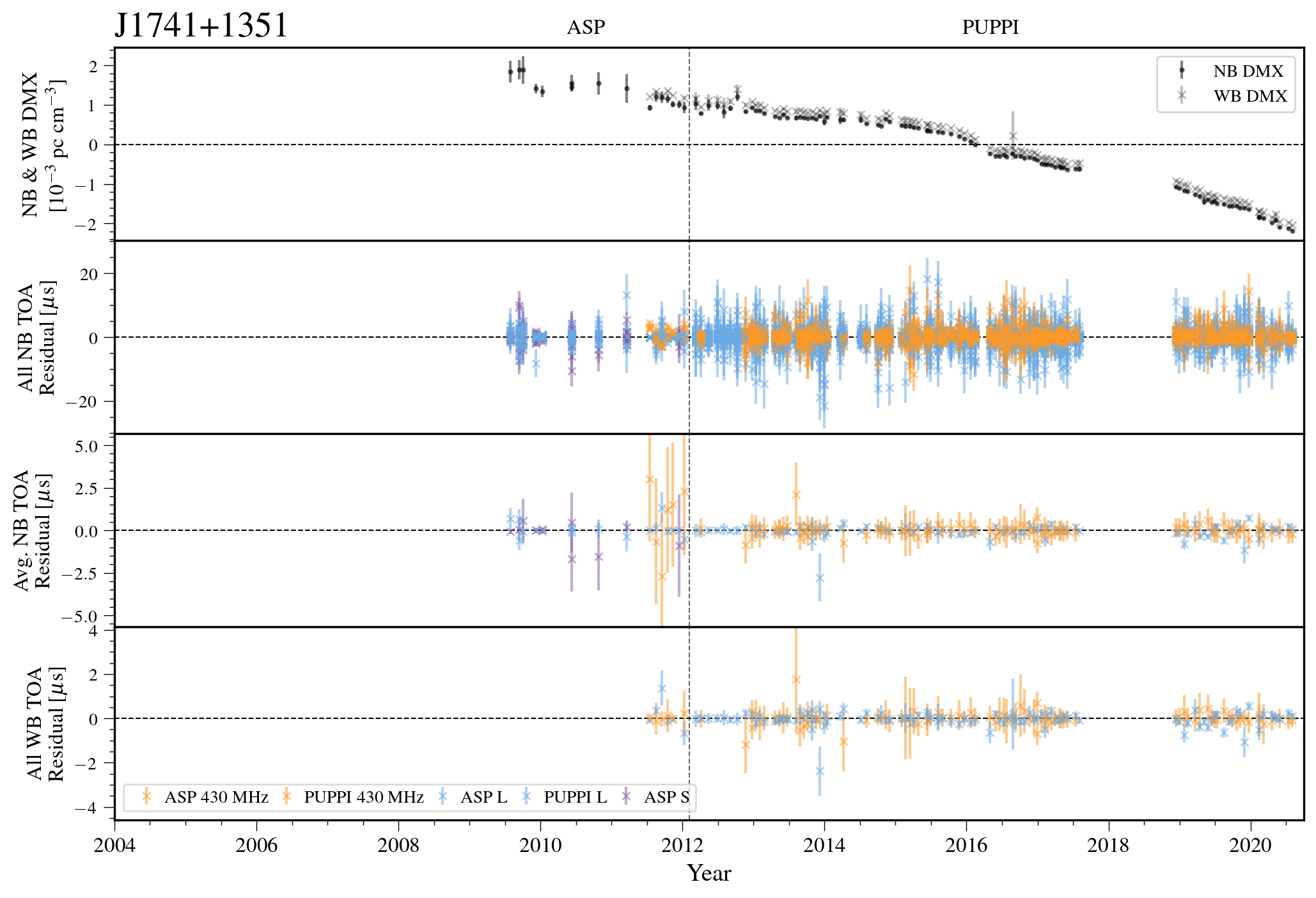
Figure 41: Narrowband and wideband timing residuals and DMX timeseries for J1741+1351. See Figure 7 for details.

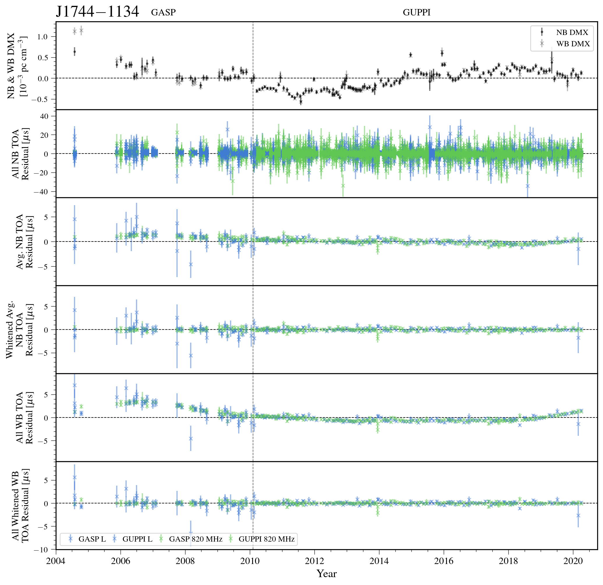
Figure 42: Narrowband and wideband timing residuals and DMX timeseries for J1744-1134. See Figure 8 for details.

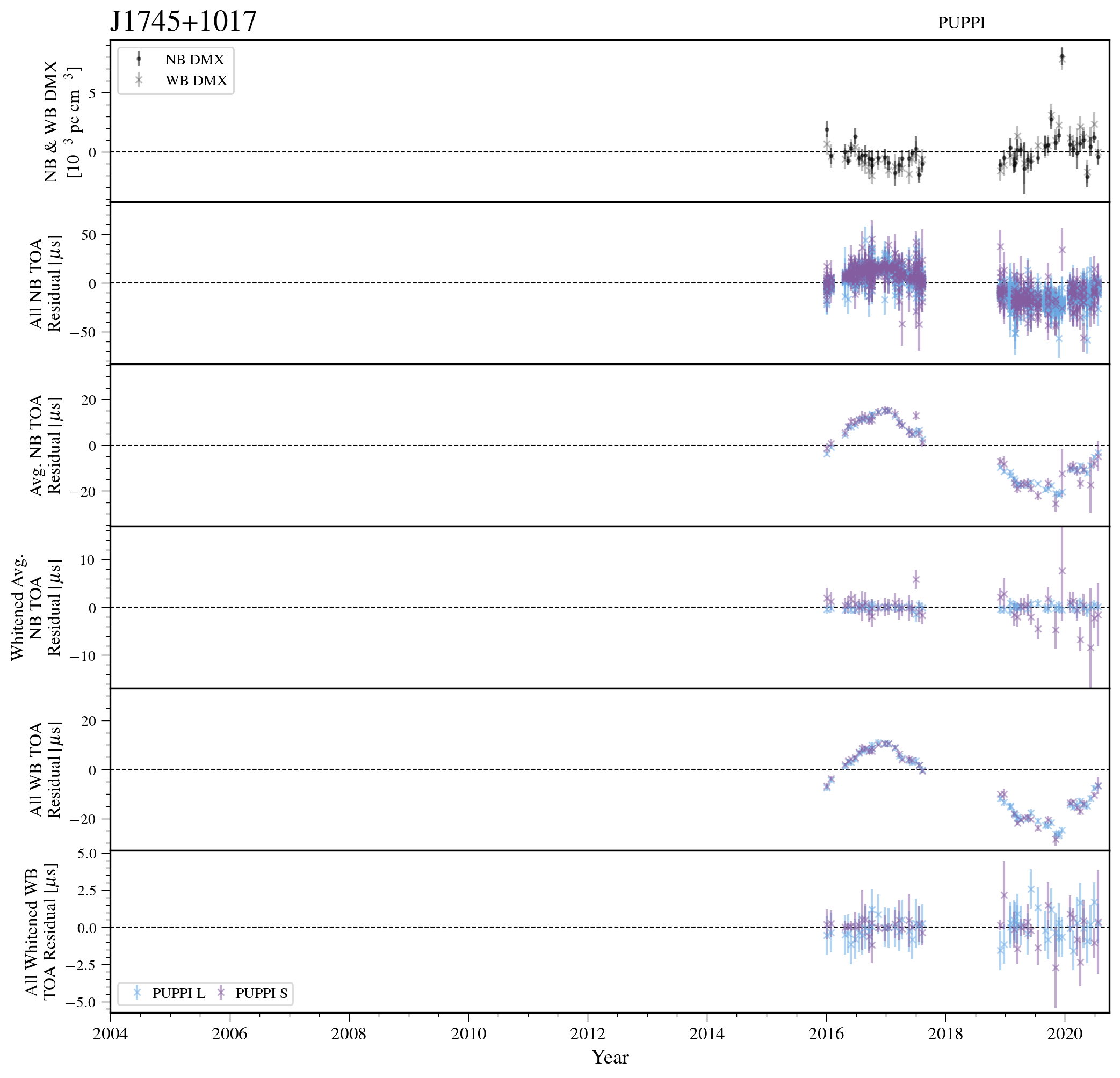
Figure 43: Narrowband and wideband timing residuals and DMX timeseries for J1745+1017. See Figure 8 for details.

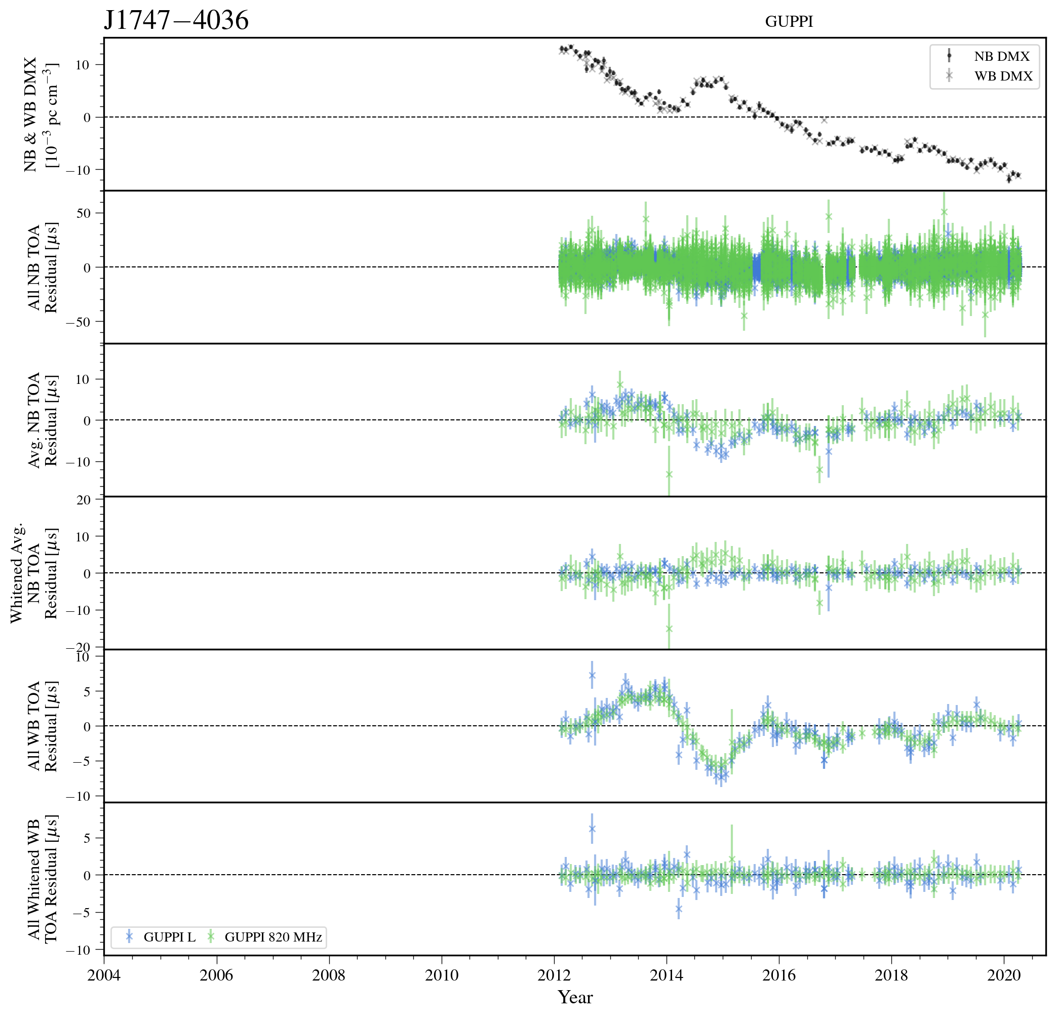
Figure 44: Narrowband and wideband timing residuals and DMX timeseries for J1747-4036. See Figure 8 for details.

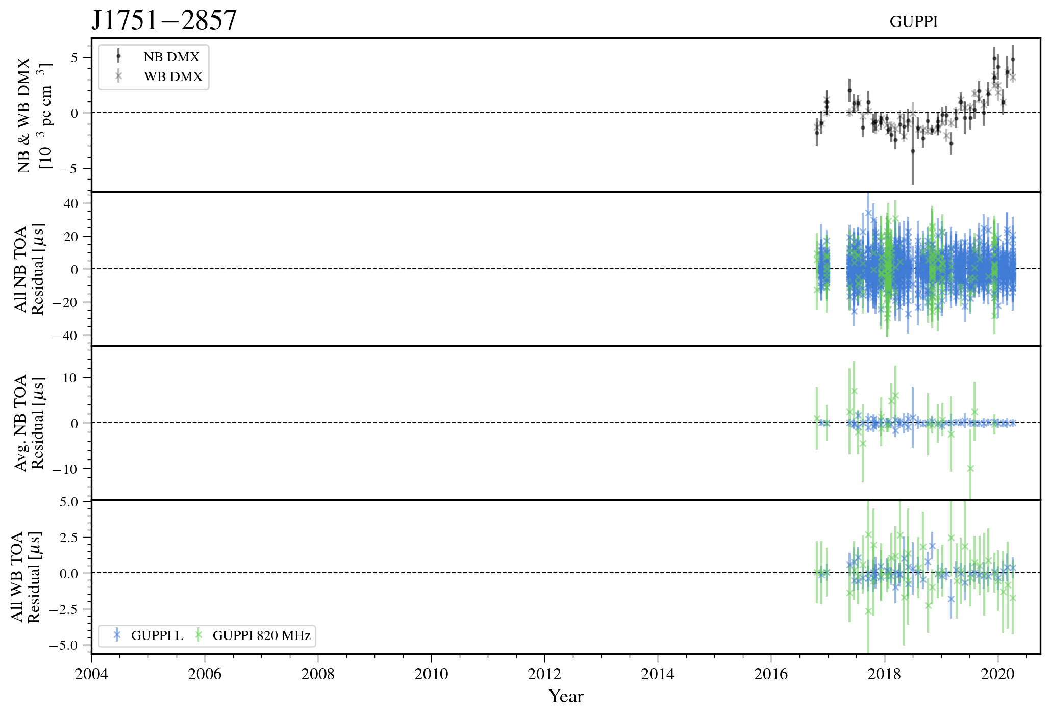
Figure 45: Narrowband and wideband timing residuals and DMX timeseries for J1751-2857. See Figure 7 for details.

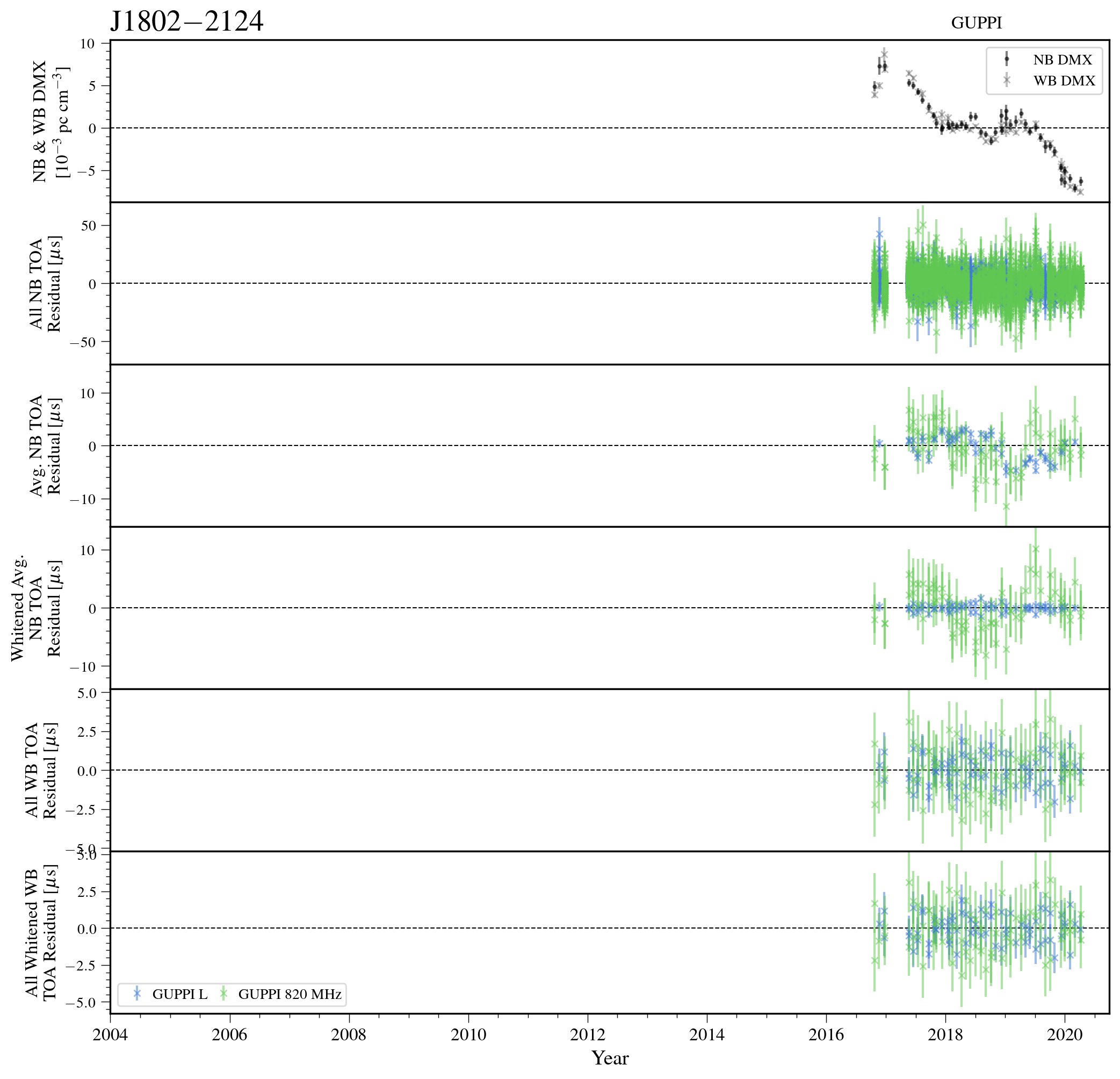
Figure 46: Narrowband and wideband timing residuals and DMX timeseries for J1802-2124. See Figure 8 for details.

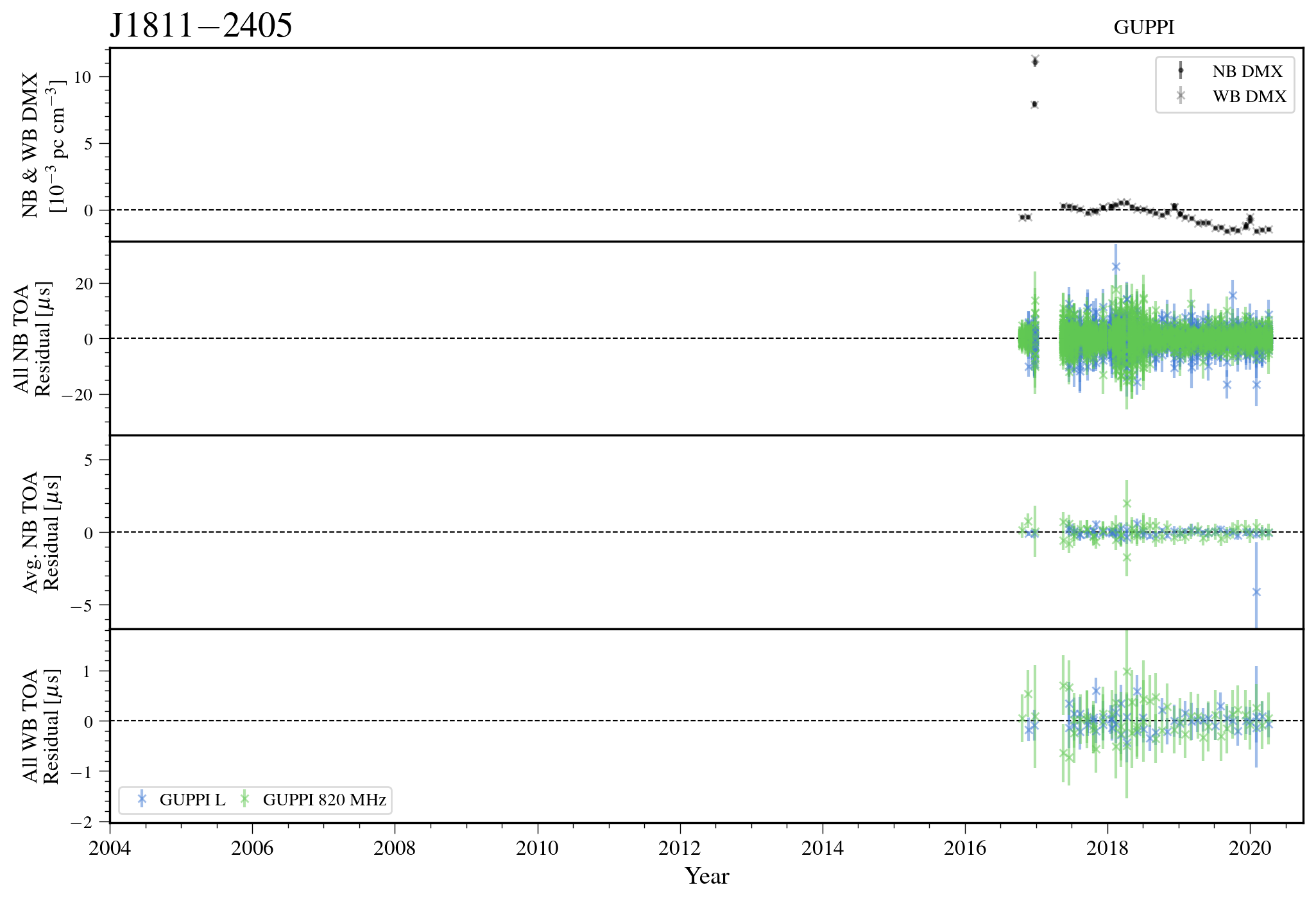
Figure 47: Narrowband and wideband timing residuals and DMX timeseries for J1811-2405. See Figure 7 for details.

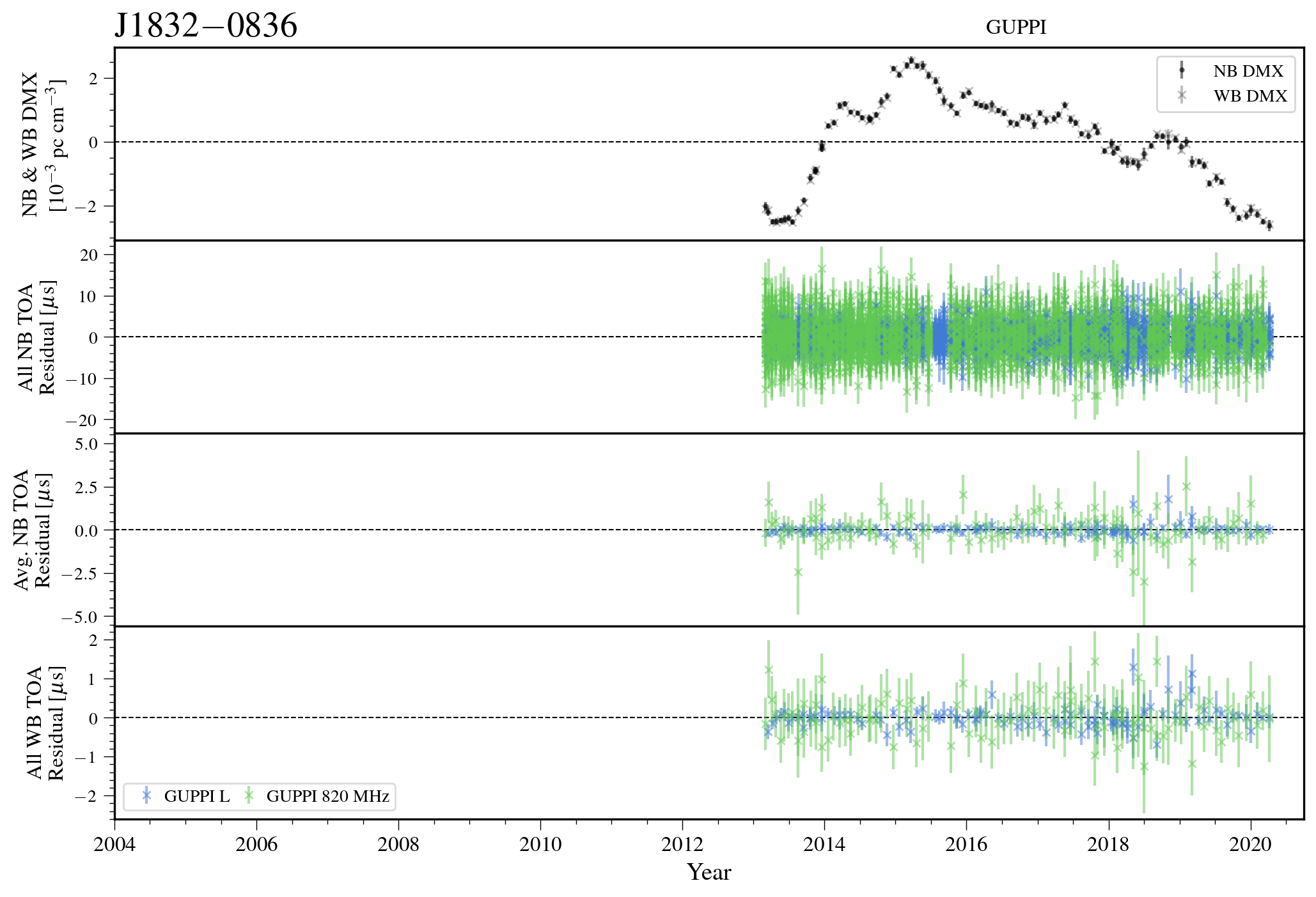
Figure 48: Narrowband and wideband timing residuals and DMX timeseries for J1832-0836. See Figure 7 for details.

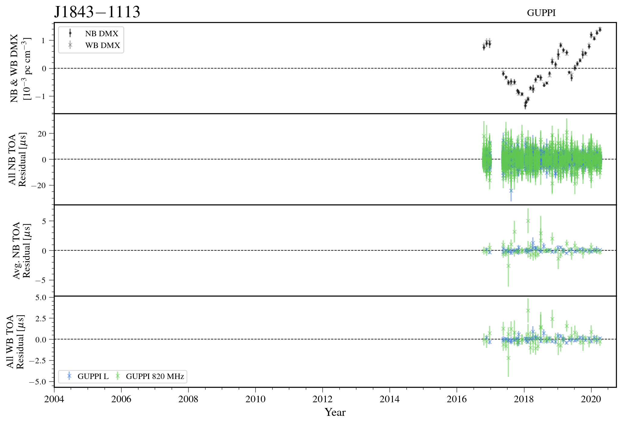
Figure 49: Narrowband and wideband timing residuals and DMX timeseries for J1843-1113. See Figure 7 for details.

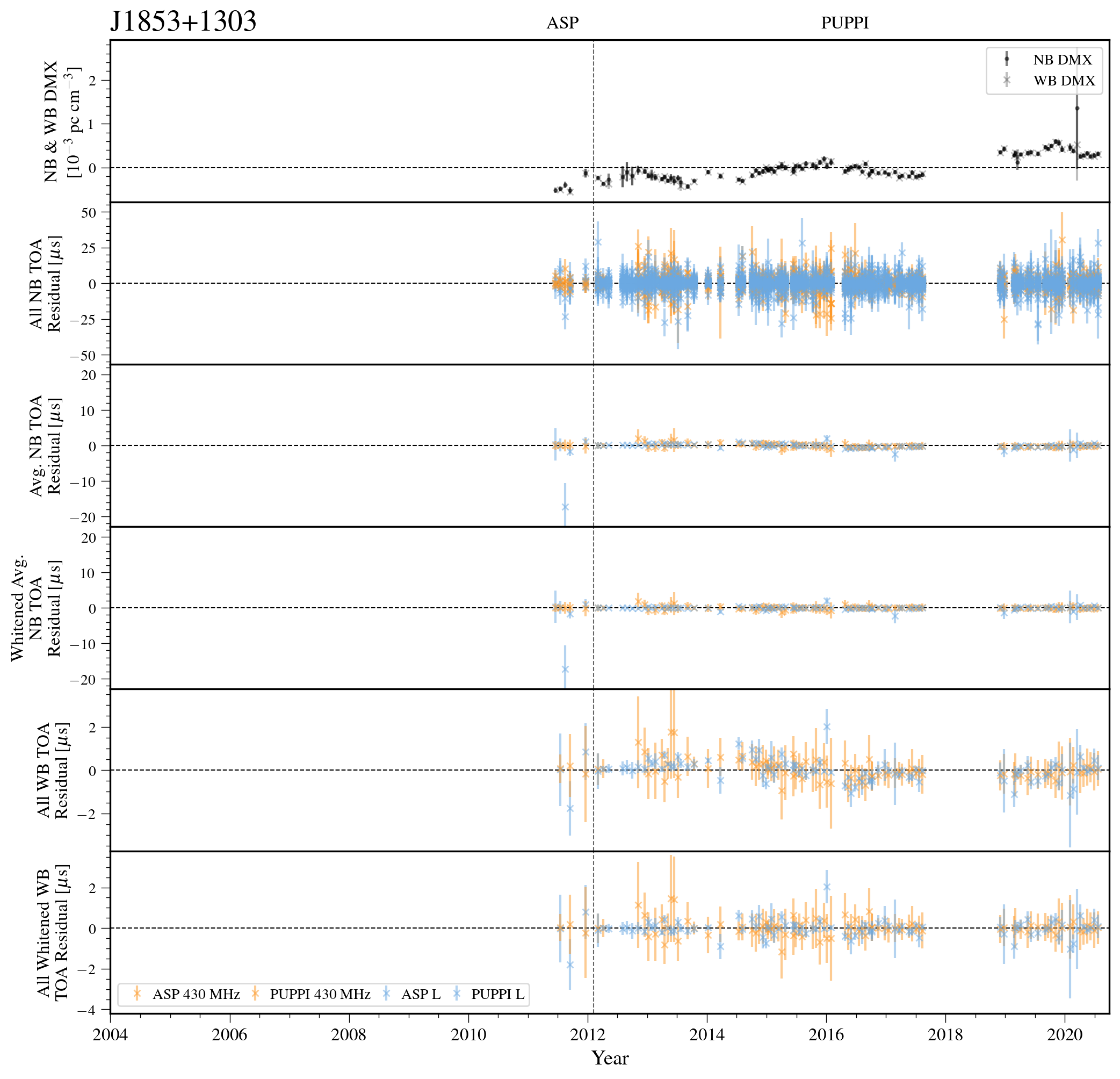
Figure 50: Narrowband and wideband timing residuals and DMX timeseries for J1853+1303. See Figure 8 for details.

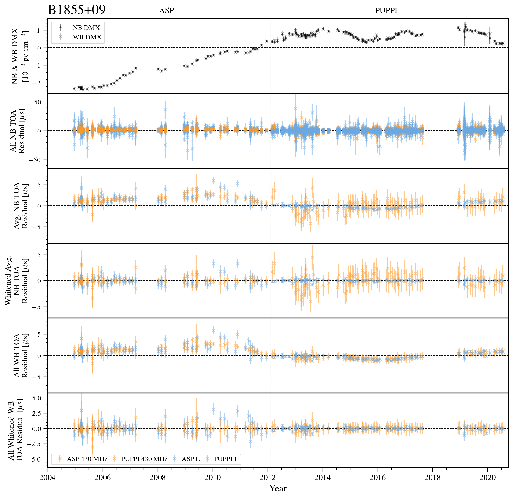
Figure 51: Narrowband and wideband timing residuals and DMX timeseries for B1855+09. See Figure 8 for details.

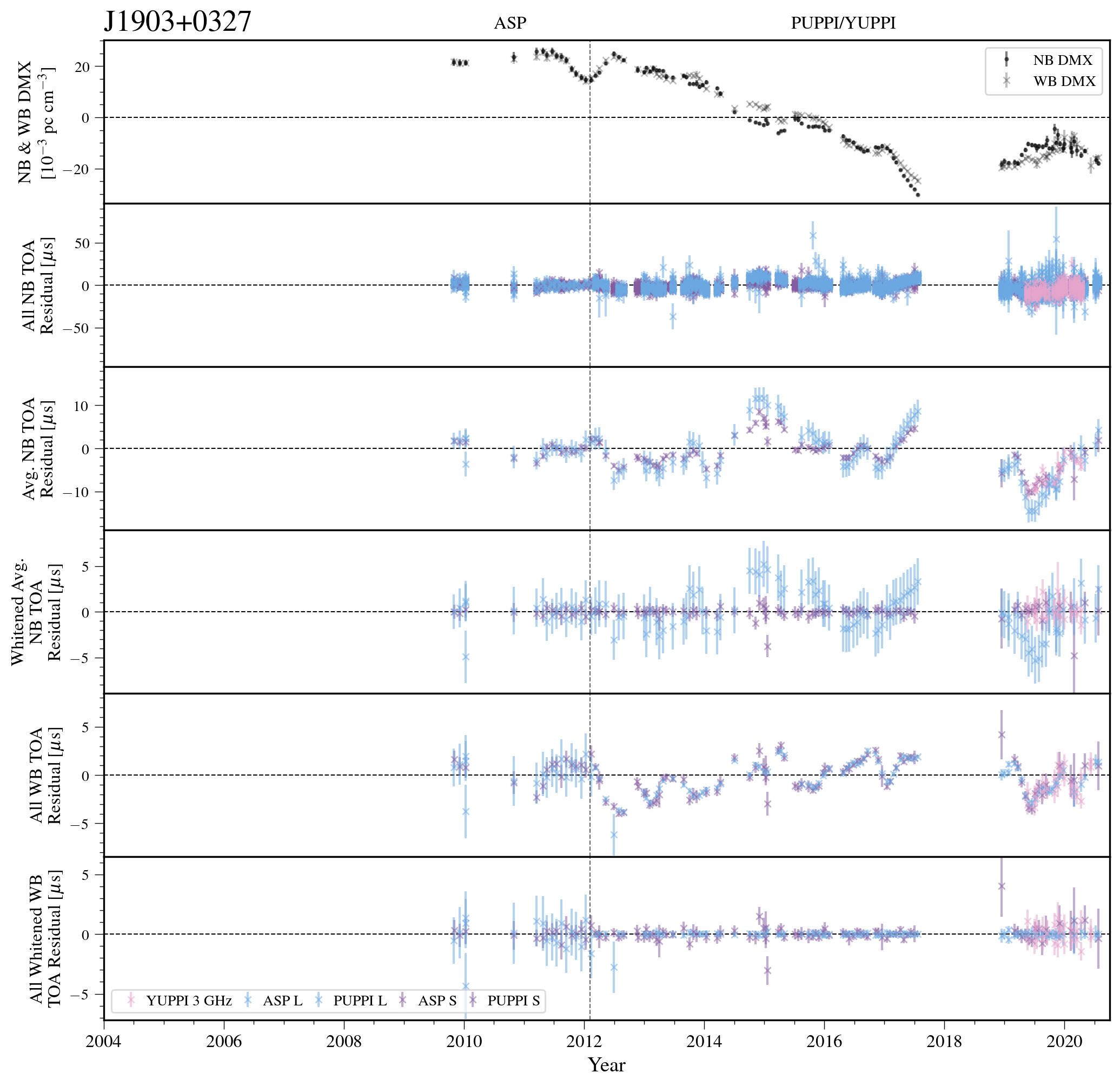
Figure 52: Narrowband and wideband timing residuals and DMX timeseries for J1903+0327. See Figure 8 for details.

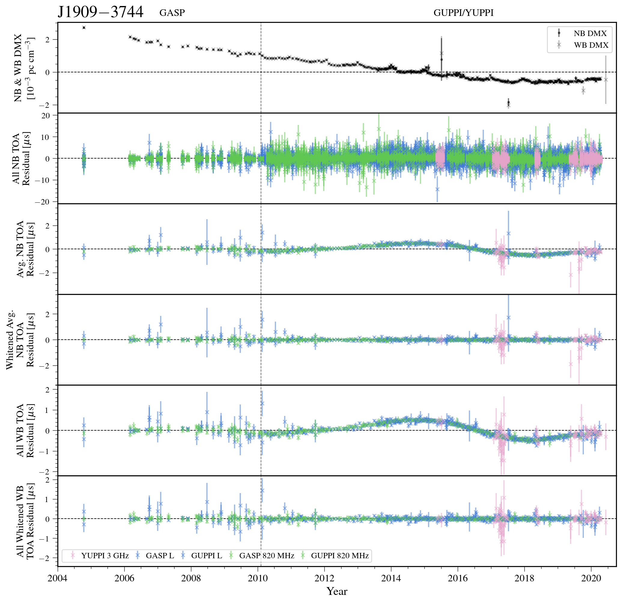
Figure 53: Narrowband and wideband timing residuals and DMX timeseries for J1909-3744. See Figure 8 for details.

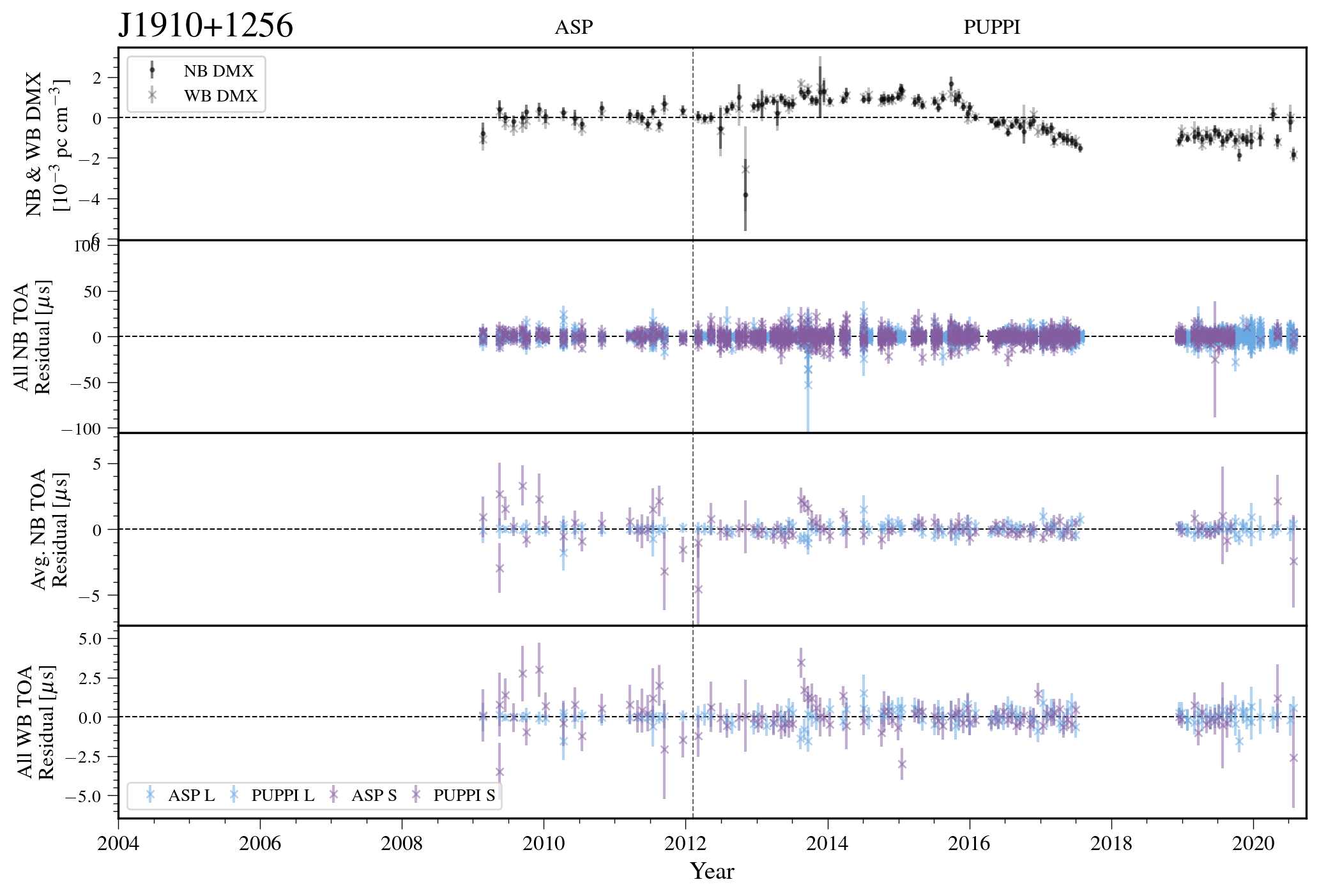
Figure 54: Narrowband and wideband timing residuals and DMX timeseries for J1910+1256. See Figure 7 for details.

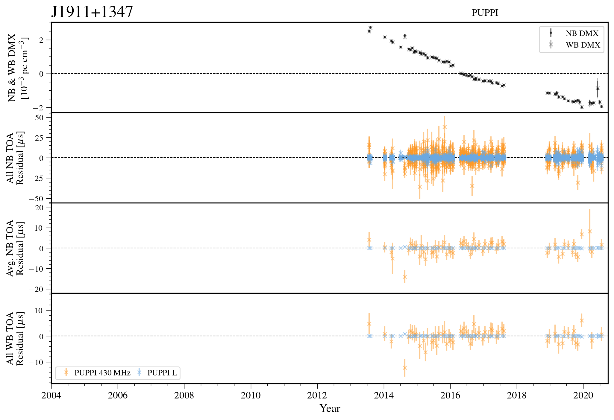
Figure 55: Narrowband and wideband timing residuals and DMX timeseries for J1911+1347. See Figure 7 for details.

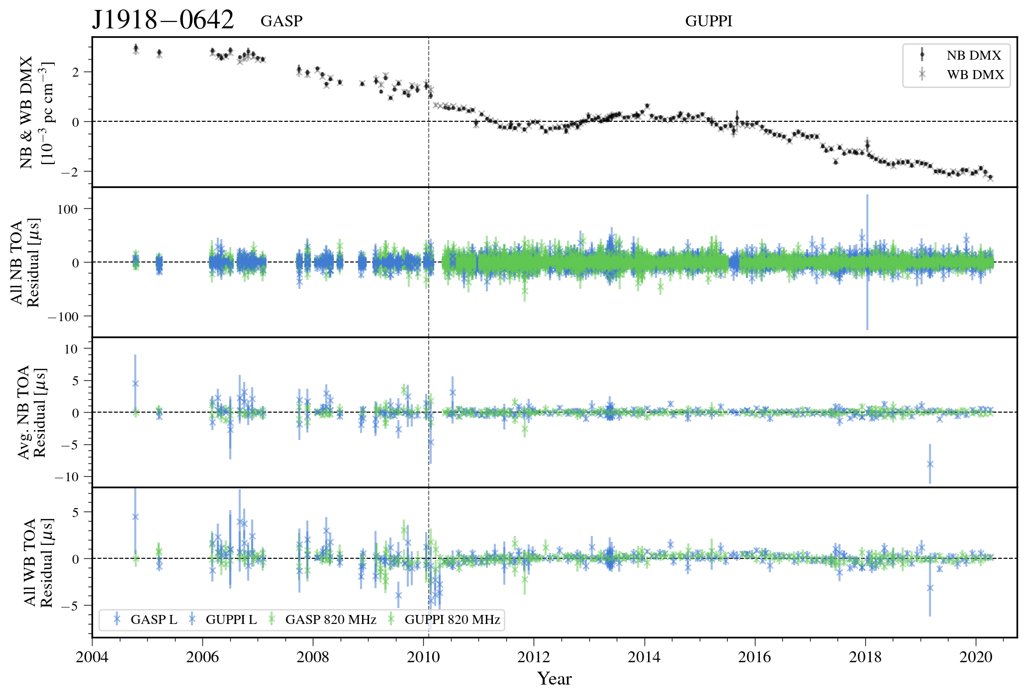
Figure 56: Narrowband and wideband timing residuals and DMX timeseries for J1918-0642. See Figure 7 for details.

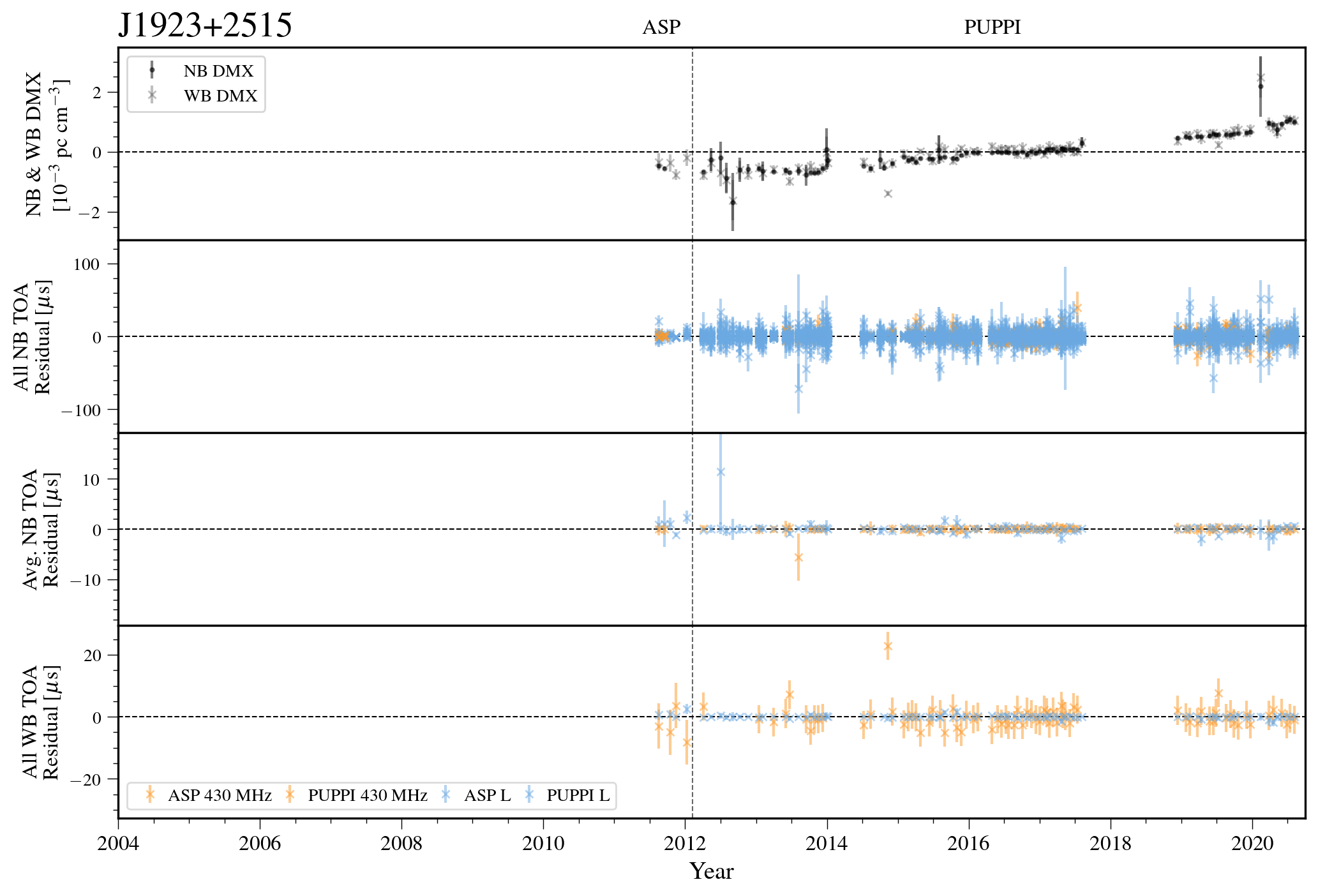
Figure 57: Narrowband and wideband timing residuals and DMX timeseries for J1923+2515. See Figure 7 for details.

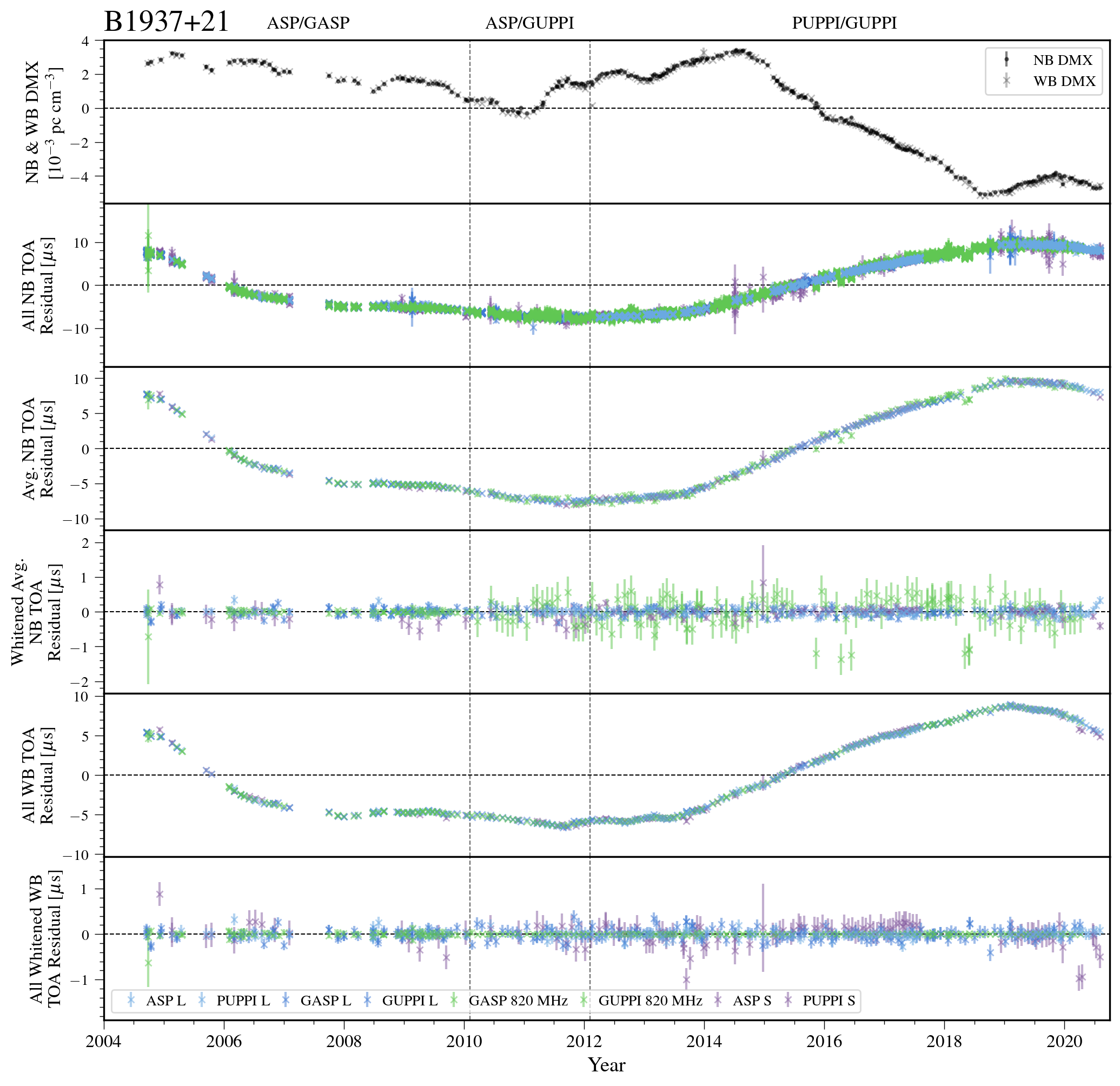
Figure 58: Narrowband and wideband timing residuals and DMX timeseries for B1937+21. See Figure 8 for details.

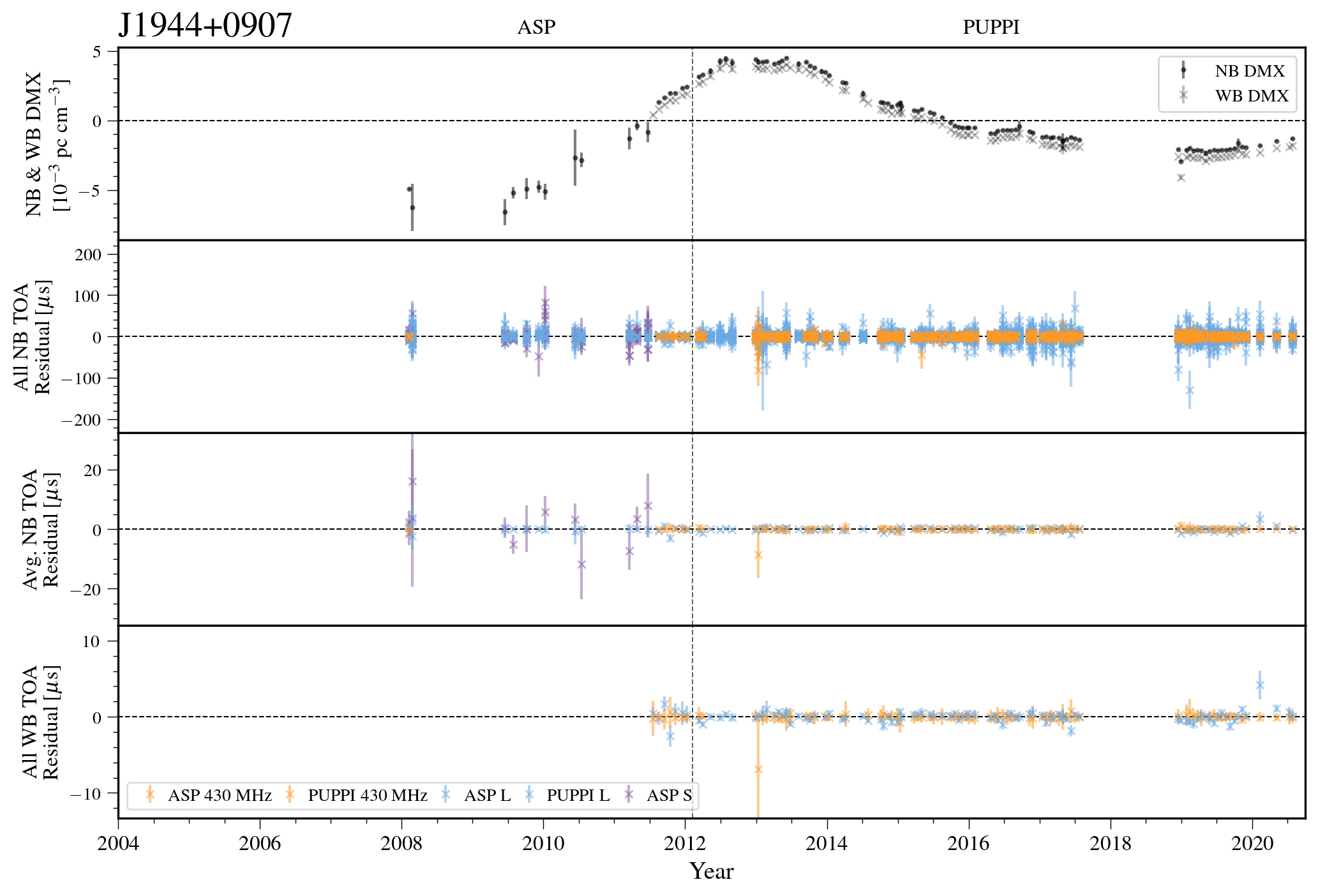
Figure 59: Narrowband and wideband timing residuals and DMX timeseries for J1944+0907. See Figure 7 for details.

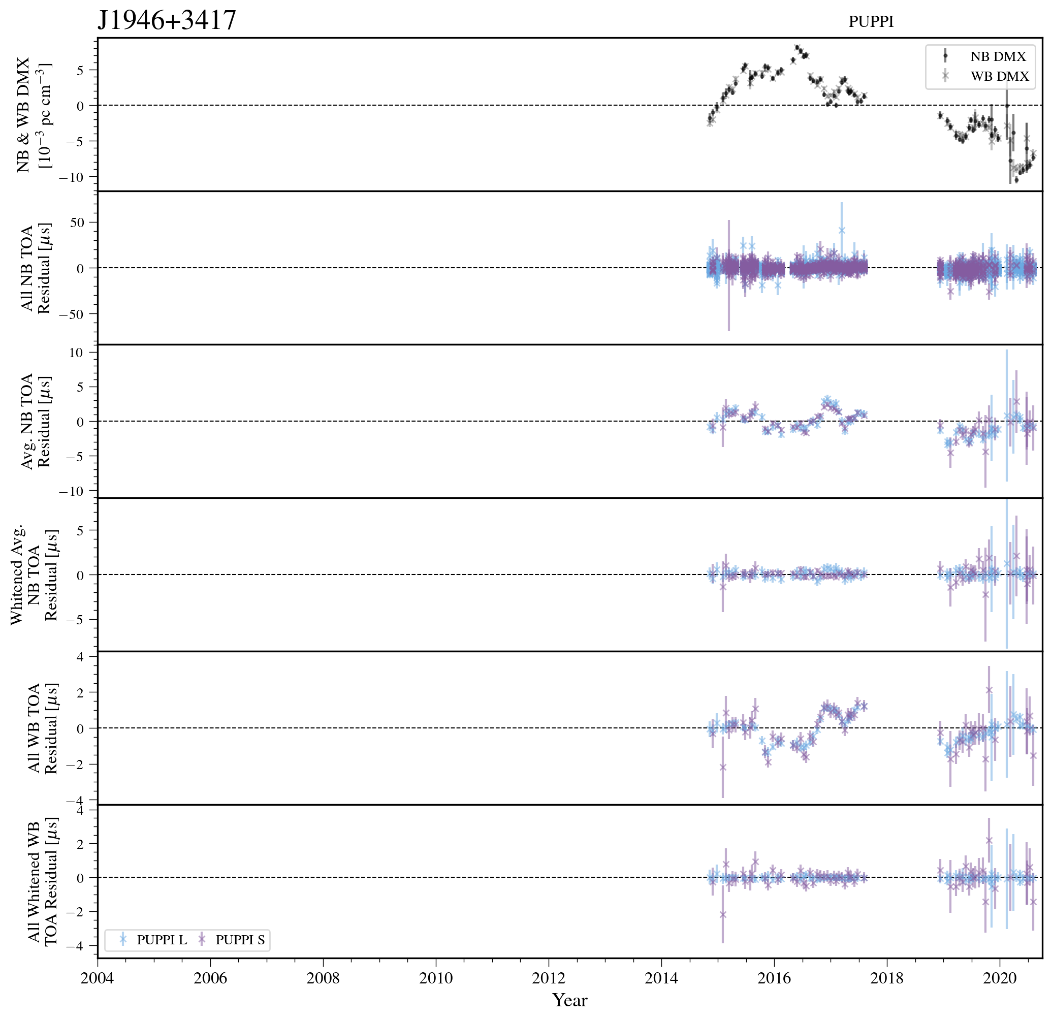
Figure 60: Narrowband and wideband timing residuals and DMX timeseries for J1946+3417. See Figure 8 for details.

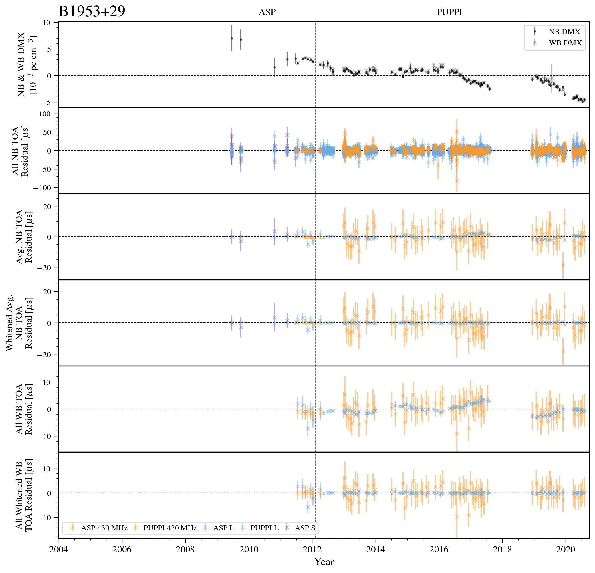
Figure 61: Narrowband and wideband timing residuals and DMX timeseries for B1953+29. See Figure 8 for details.

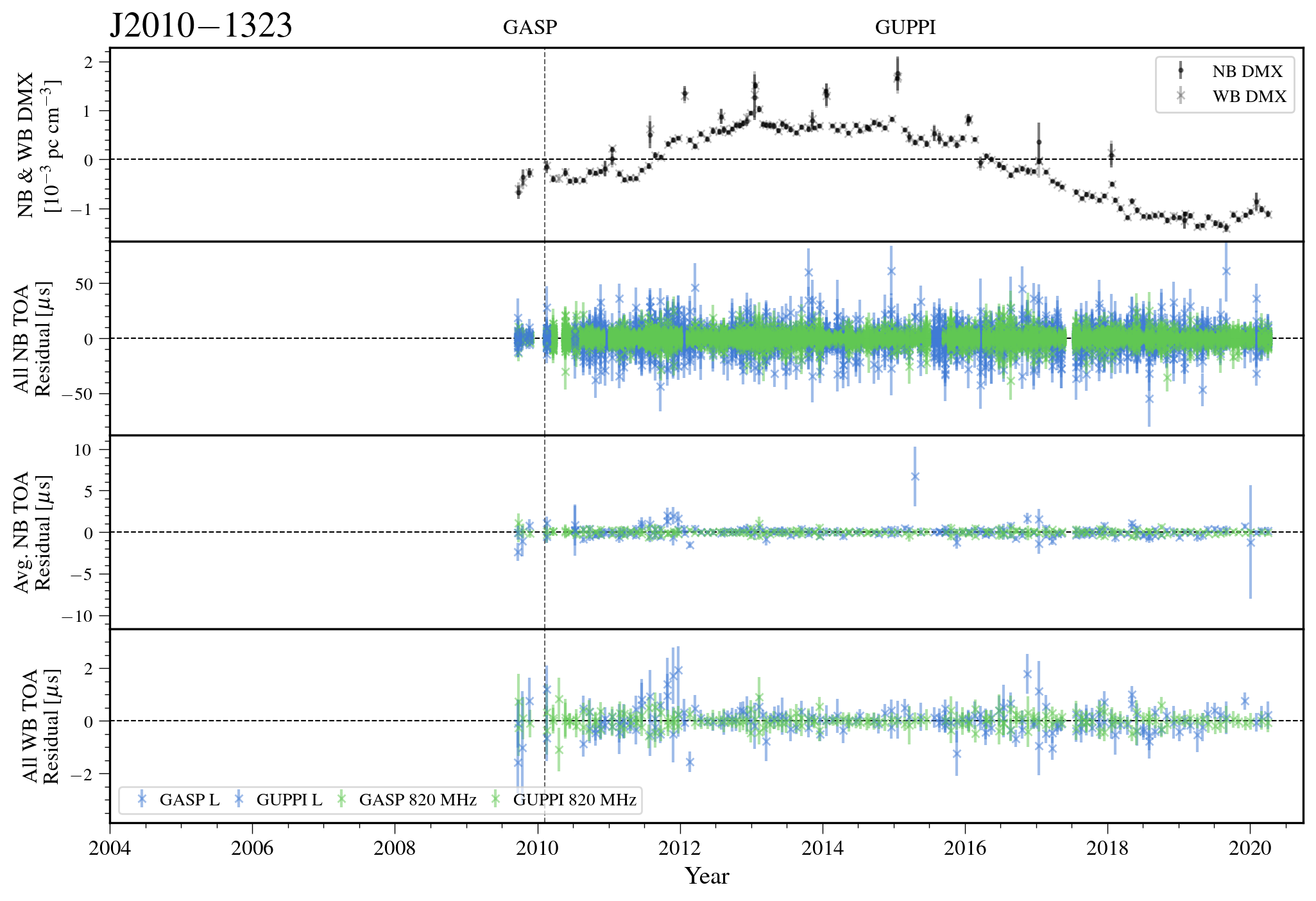
Figure 62: Narrowband and wideband timing residuals and DMX timeseries for J2010-1323. See Figure 7 for details.

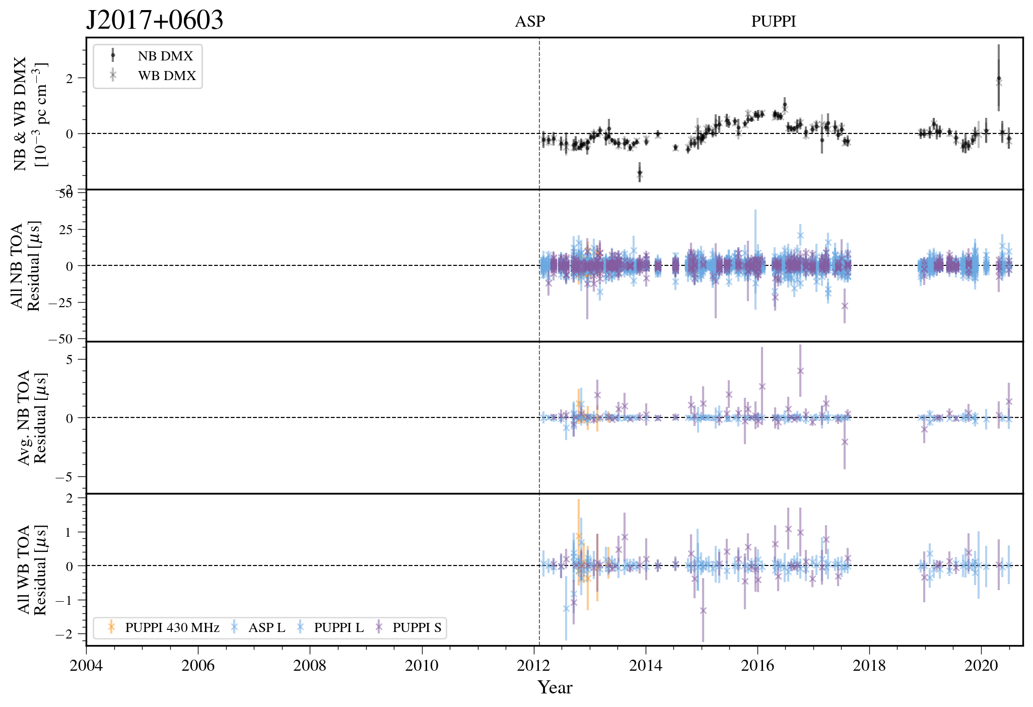
Figure 63: Narrowband and wideband timing residuals and DMX timeseries for J2017+0603. See Figure 7 for details.

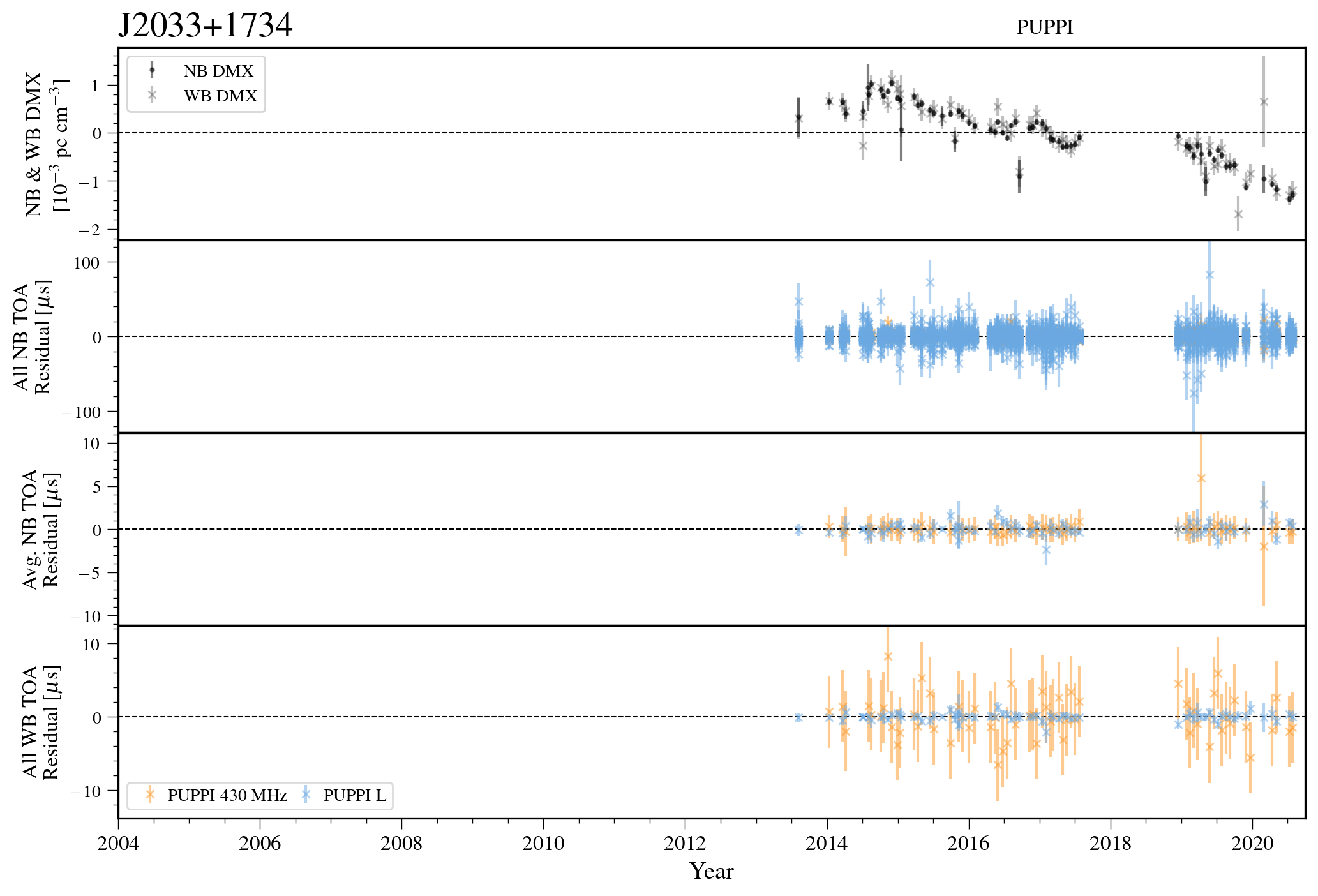
Figure 64: Narrowband and wideband timing residuals and DMX timeseries for J2033+1734. See Figure 7 for details.

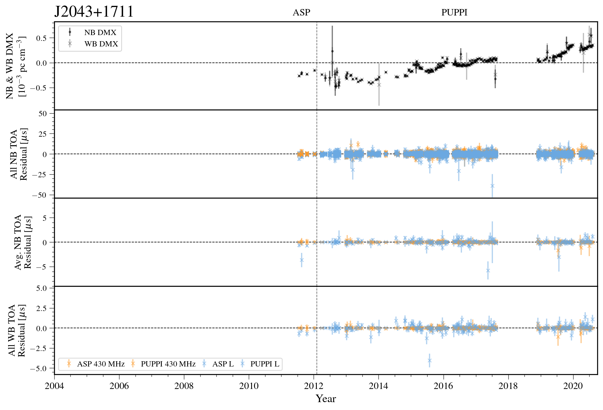
Figure 65: Narrowband and wideband timing residuals and DMX timeseries for J2043+1711. See Figure 7 for details.

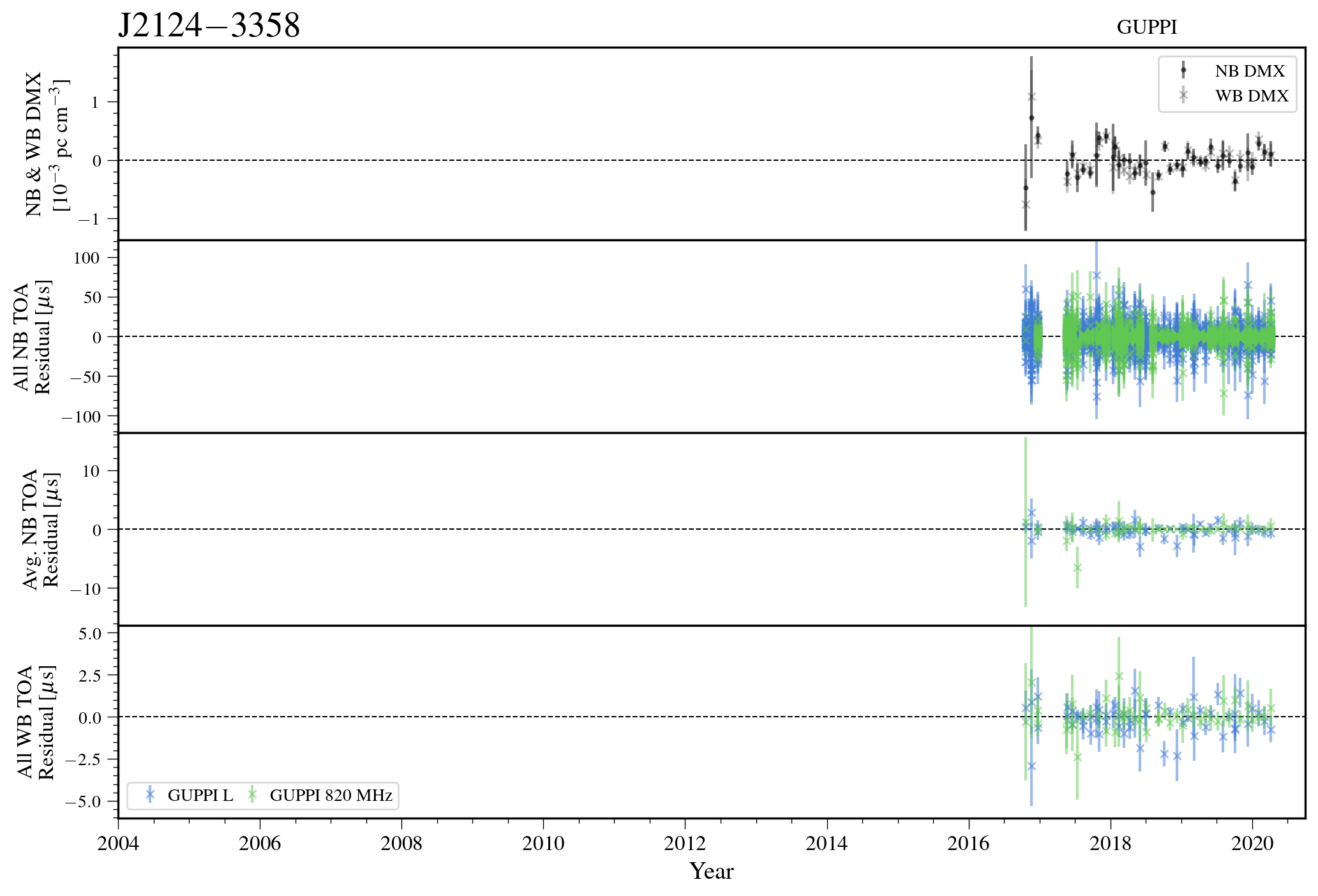
Figure 66: Narrowband and wideband timing residuals and DMX timeseries for J2124-3358. See Figure 7 for details.

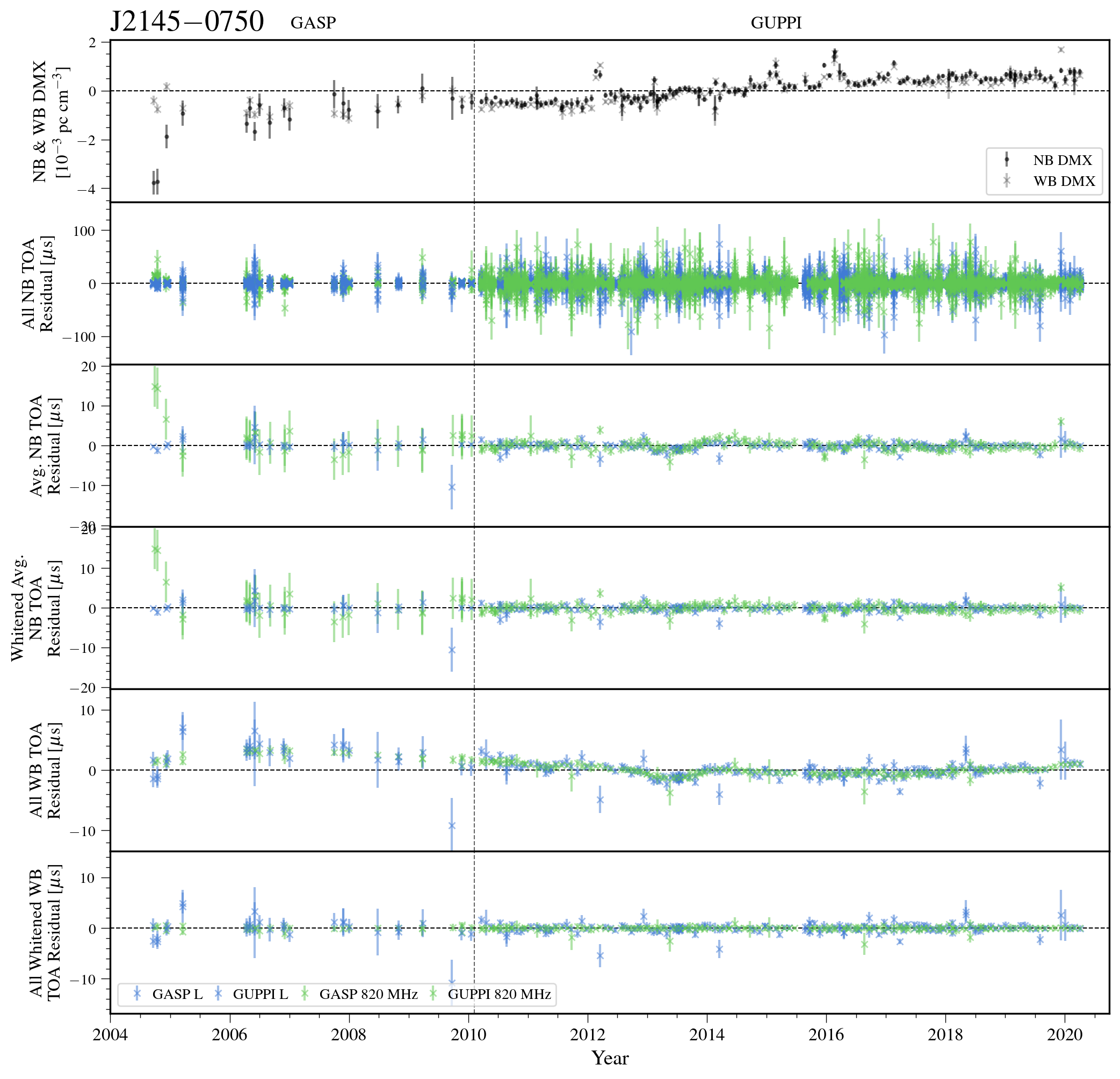
Figure 67: Narrowband and wideband timing residuals and DMX timeseries for J2145-0750. See Figure 8 for details.

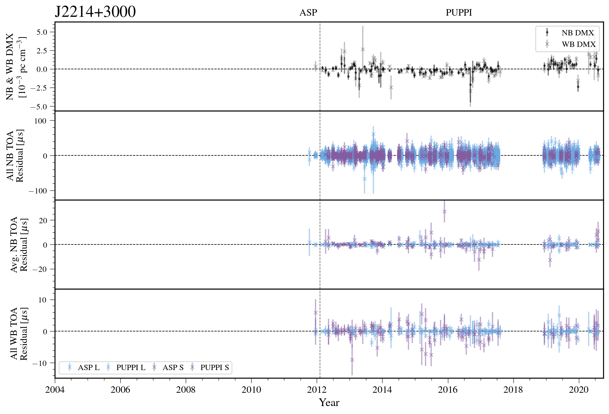
Figure 68: Narrowband and wideband timing residuals and DMX timeseries for J2214+3000. See Figure 7 for details.

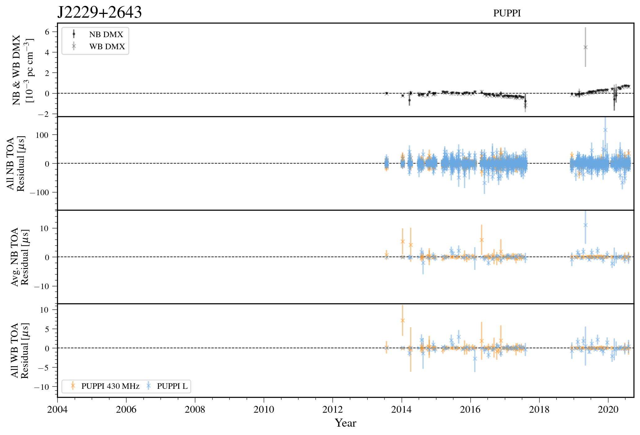
Figure 69: Narrowband and wideband timing residuals and DMX timeseries for J2229+2643. See Figure 7 for details.

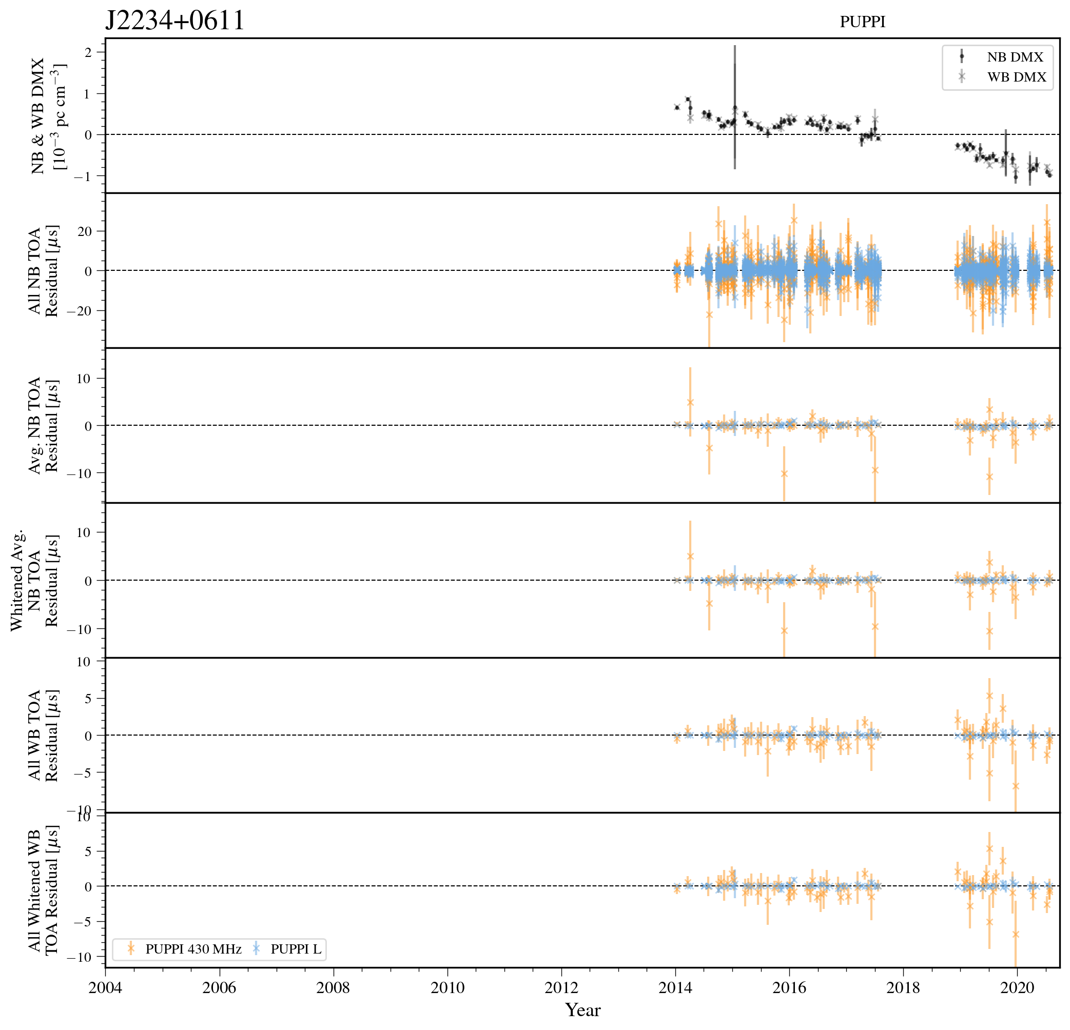
Figure 70: Narrowband and wideband timing residuals and DMX timeseries for J2234+0611. See Figure 8 for details.

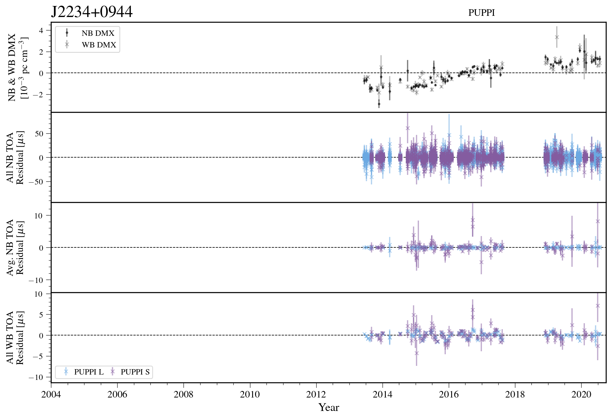
Figure 71: Narrowband and wideband timing residuals and DMX timeseries for J2234+0944. See Figure 7 for details.

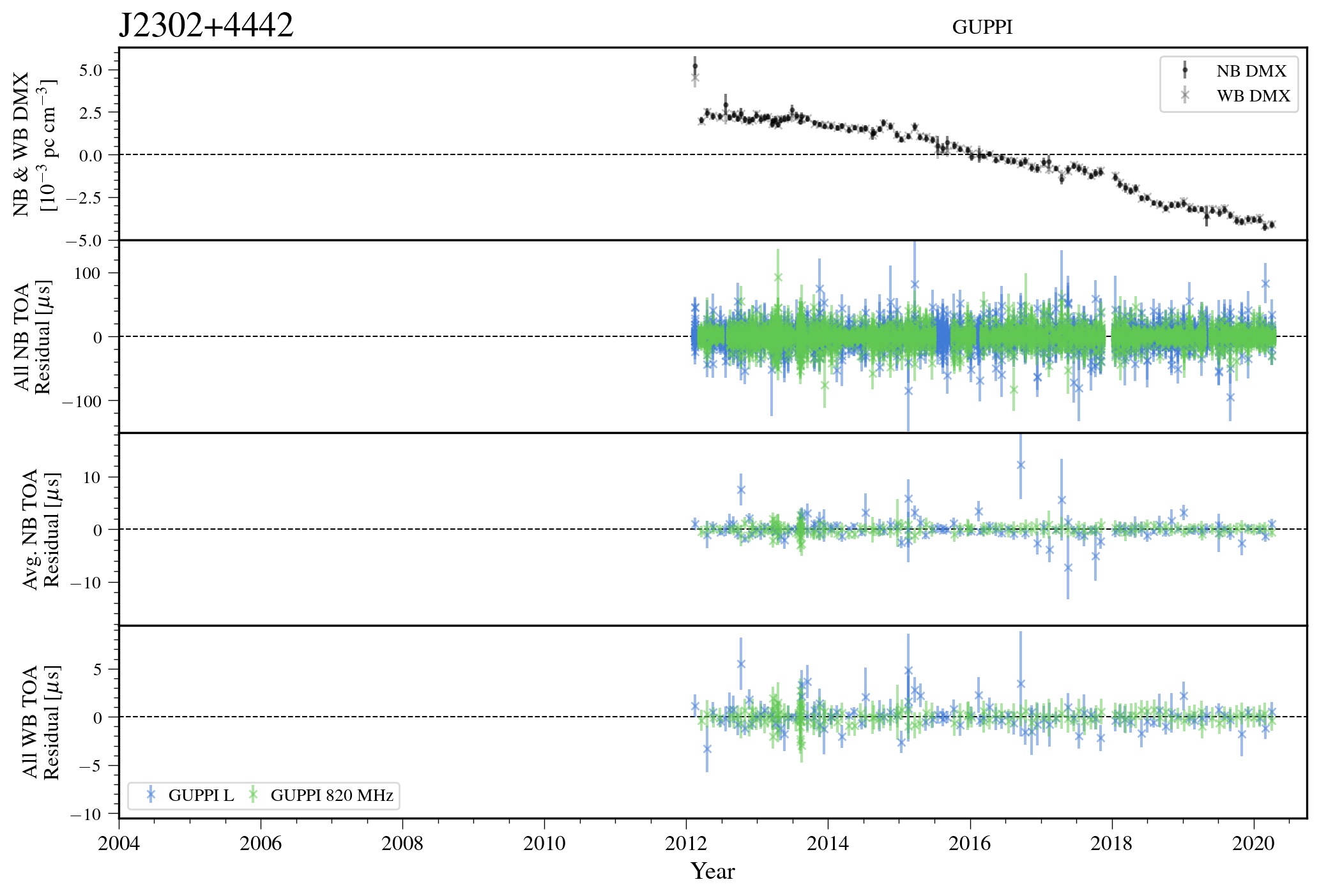
Figure 72: Narrowband and wideband timing residuals and DMX timeseries for J2302+4442. See Figure 7 for details.

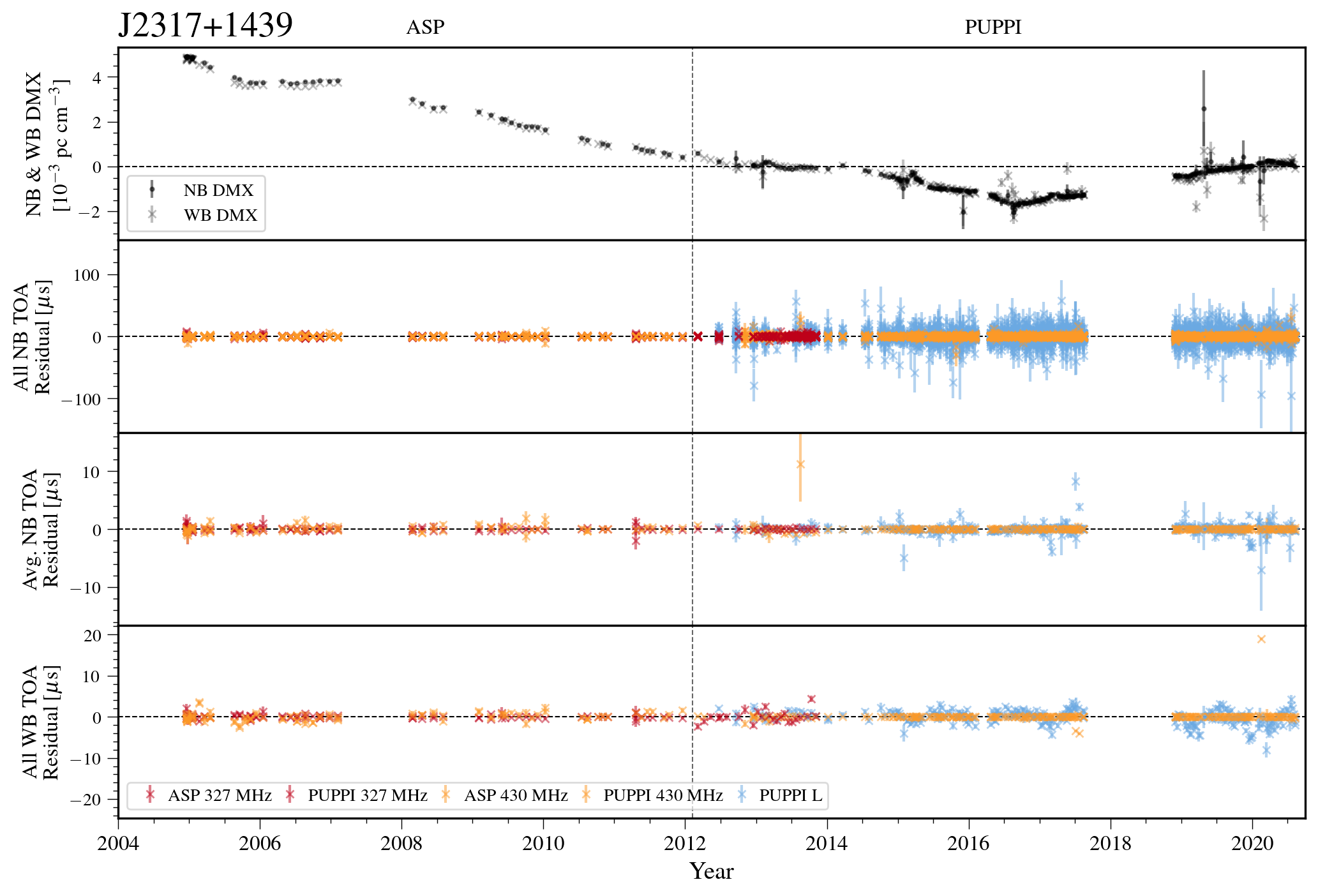
Figure 73: Narrowband and wideband timing residuals and DMX timeseries for J2317+1439. See Figure 7 for details.

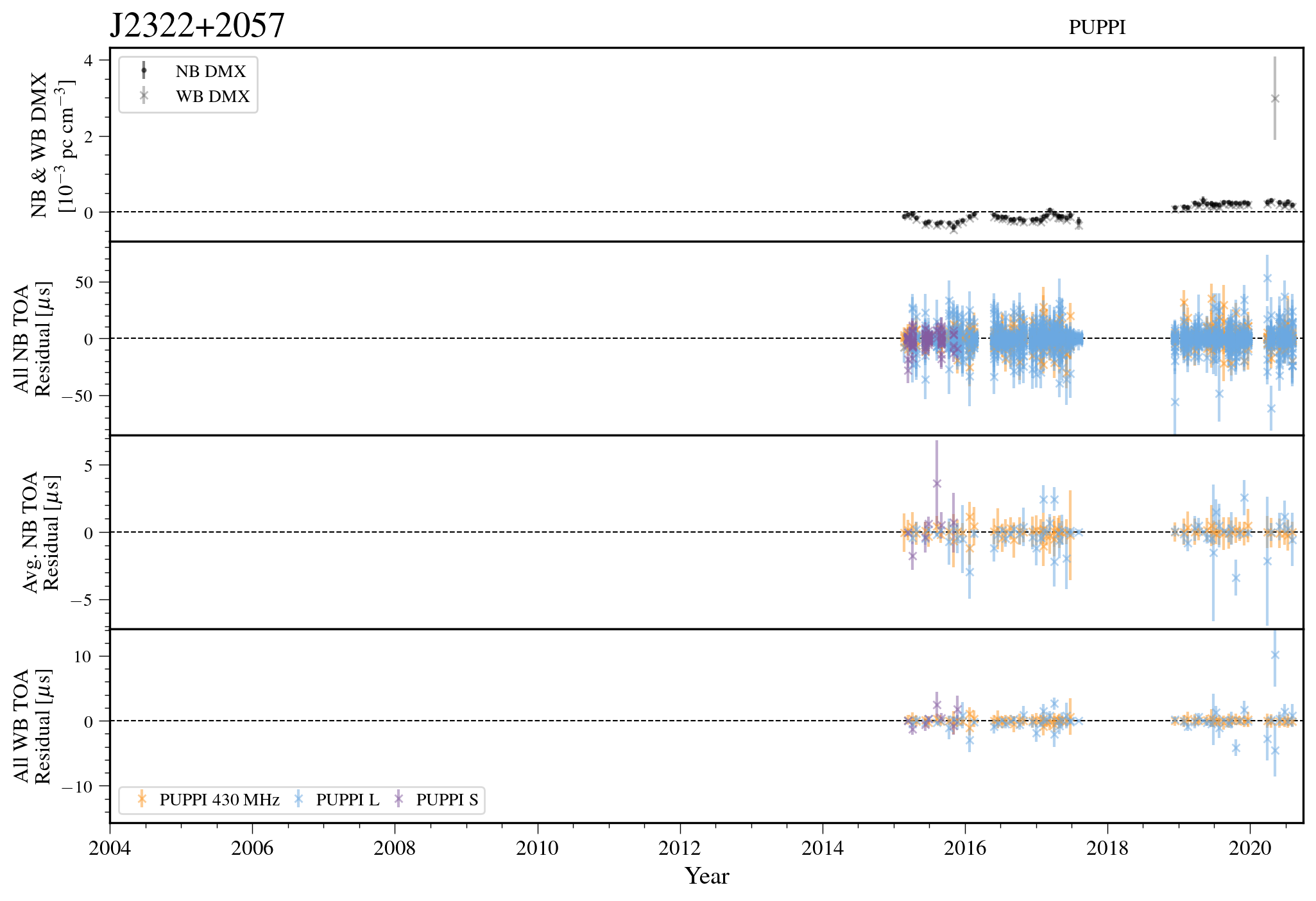
Figure 74: Narrowband and wideband timing residuals and DMX timeseries for J2322+2057. See Figure 7 for details.

References

- Afzal et al. (2023) Afzal, A., Agazie, G., Alam, M. F., et al. 2023
- Agazie et al. (2023a) Agazie, G., Alam, M. F., Anumarlapudi, A., et al. 2023a
- Agazie et al. (2023b) Agazie, G., Anumarlapudi, A., Archibald, A. M., Arzoumanian, Z., & Others. 2023b, doi: 10.3847/2041-8213/acdac6
- Agazie et al. (2023c) Agazie, G., Anumarlapudi, A., Archibald, A. M., & Others. 2023c, doi: 10.3847/2041-8213/acda88
- Alam et al. (2021a) Alam, M. F., Arzoumanian, Z., Baker, P. T., et al. 2021a, ApJS, 252, 4, doi: 10.3847/1538-4365/abc6a0
- Alam et al. (2021b) —. 2021b, ApJS, 252, 5, doi: 10.3847/1538-4365/abc6a1
- Alpar et al. (1982) Alpar, M. A., Cheng, A. F., Ruderman, M. A., & Shaham, J. 1982, Nature, 300, 728, doi: 10.1038/300728a0
- Arzoumanian et al. (1996) Arzoumanian, Z., Joshi, K., Rasio, F. A., & Thorsett, S. E. 1996, in Astronomical Society of the Pacific Conference Series, Vol. 105, IAU Colloq. 160: Pulsars: Problems and Progress, ed. S. Johnston, M. A. Walker, & M. Bailes, 525–530, doi: 10.48550/arXiv.astro-ph/9605141
- Arzoumanian et al. (2015) Arzoumanian, Z., Brazier, A., Burke-Spolaor, S., et al. 2015, ApJ, 813, 65, doi: 10.1088/0004-637X/813/1/65
- Arzoumanian et al. (2018) —. 2018, ArXiv e-prints. https://arxiv.org/abs/1801.01837
- Arzoumanian et al. (2020) Arzoumanian, Z., Baker, P. T., Blumer, H., et al. 2020, ApJ, 905, L34, doi: 10.3847/2041-8213/abd401
- Arzoumanian et al. (2021a) —. 2021a, ApJ, 923, L22, doi: 10.3847/2041-8213/ac401c
- Arzoumanian et al. (2021b) —. 2021b, Phys. Rev. Lett., 127, 251302, doi: 10.1103/PhysRevLett.127.251302
- Arzoumanian et al. (2023) Arzoumanian, Z., Baker, P. T., Blecha, L., et al. 2023, arXiv e-prints, arXiv:2301.03608, doi: 10.48550/arXiv.2301.03608
- Astropy Collaboration et al. (2022) Astropy Collaboration, Price-Whelan, A. M., Lim, P. L., et al. 2022, apj, 935, 167, doi: 10.3847/1538-4357/ac7c74
- Backer et al. (1982) Backer, D. C., Kulkarni, S. R., Heiles, C., Davis, M. M., & Goss, W. M. 1982, Nature, 300, 615, doi: 10.1038/300615a0
- Barr et al. (2013) Barr, E. D., Guillemot, L., Champion, D. J., et al. 2013, MNRAS, 429, 1633, doi: 10.1093/mnras/sts449
- Blandford & Teukolsky (1976) Blandford, R., & Teukolsky, S. A. 1976, ApJ, 205, 580, doi: 10.1086/154315
- Camilo et al. (2015) Camilo, F., Kerr, M., Ray, P. S., et al. 2015, ApJ, 810, 85, doi: 10.1088/0004-637X/810/2/85
- Chen et al. (2021) Chen, S., Caballero, R. N., Guo, Y. J., et al. 2021, MNRAS, 508, 4970, doi: 10.1093/mnras/stab2833
- CHIME/Pulsar Collaboration et al. (2021) CHIME/Pulsar Collaboration, Amiri, M., Bandura, K. M., et al. 2021, ApJS, 255, 5, doi: 10.3847/1538-4365/abfdcb
- conda-forge Community (2015) conda-forge Community. 2015, The conda-forge Project: Community-based Software Distribution Built on the conda Package Format and Ecosystem, Zenodo, doi: 10.5281/zenodo.4774216
- Cromartie et al. (2020) Cromartie, H. T., Fonseca, E., Ransom, S. M., et al. 2020, Nature Astronomy, 4, 72, doi: 10.1038/s41550-019-0880-2
- Damour & Deruelle (1985) Damour, T., & Deruelle, N. 1985, Ann. Inst. Henri Poincaré Phys. Théor., Vol. 43, No. 1, p. 107 - 132, 43, 107
- Damour & Deruelle (1986) —. 1986, Ann. Inst. Henri Poincaré Phys. Théor., Vol. 44, No. 3, p. 263 - 292, 44, 263
- Damour & Taylor (1992) Damour, T., & Taylor, J. H. 1992, Phys. Rev. D, 45, 1840, doi: 10.1103/PhysRevD.45.1840
- Demorest (2007) Demorest, P. B. 2007, PhD thesis, University of California, Berkeley
- Demorest (2018) —. 2018, nanopipe: Calibration and data reduction pipeline for pulsar timing, Astrophysics Source Code Library. http://ascl.net/1803.004
- Demorest et al. (2010) Demorest, P. B., Pennucci, T., Ransom, S. M., Roberts, M. S. E., & Hessels, J. W. T. 2010, Nature, 467, 1081, doi: 10.1038/nature09466
- Demorest et al. (2013) Demorest, P. B., Ferdman, R. D., Gonzalez, M. E., et al. 2013, ApJ, 762, 94, doi: 10.1088/0004-637X/762/2/94
- Desvignes et al. (2016) Desvignes, G., Caballero, R. N., Lentati, L., et al. 2016, MNRAS, 458, 3341, doi: 10.1093/mnras/stw483
- Detweiler (1979) Detweiler, S. 1979, ApJ, 234, 1100, doi: 10.1086/157593
- DuPlain et al. (2008) DuPlain, R., Ransom, S., Demorest, P., et al. 2008, in Proc. SPIE, Vol. 7019, Advanced Software and Control for Astronomy II, 70191D, doi: 10.1117/12.790003
- Ellis & van Haasteren (2017) Ellis, J., & van Haasteren, R. 2017, jellis18/PTMCMCSampler: Official Release, doi: 10.5281/zenodo.1037579
- Ellis et al. (2013) Ellis, J. A., Siemens, X., & van Haasteren, R. 2013, ApJ, 769, 63, doi: 10.1088/0004-637X/769/1/63
- Ellis et al. (2019) Ellis, J. A., Vallisneri, M., Taylor, S. R., & Baker, P. T. 2019, ENTERPRISE: Enhanced Numerical Toolbox Enabling a Robust PulsaR Inference SuitE. http://ascl.net/1912.015
- Faulkner et al. (2004) Faulkner, A. J., Stairs, I. H., Kramer, M., et al. 2004, MNRAS, 355, 147, doi: 10.1111/j.1365-2966.2004.08310.x
- Fonseca et al. (2016) Fonseca, E., Pennucci, T. T., Ellis, J. A., et al. 2016, ApJ, 832, 167, doi: 10.3847/0004-637X/832/2/167
- Fonseca et al. (2021) Fonseca, E., Cromartie, H. T., Pennucci, T. T., et al. 2021, ApJ, 915, L12, doi: 10.3847/2041-8213/ac03b8
- Foster & Backer (1990) Foster, R. S., & Backer, D. C. 1990, ApJ, 361, 300, doi: 10.1086/169195
- Freedman et al. (2021) Freedman, G., Johnson, A. D., & Glaser, J. P. 2021, enterprise_outliers. https://github.com/nanograv/enterprise_outliers
- Freire & Wex (2010) Freire, P. C. C., & Wex, N. 2010, MNRAS, 409, 199, doi: 10.1111/j.1365-2966.2010.17319.x
- Goncharov et al. (2021) Goncharov, B., Reardon, D. J., Shannon, R. M., et al. 2021, MNRAS, 502, 478, doi: 10.1093/mnras/staa3411
- Granger & Pérez (2021) Granger, B. E., & Pérez, F. 2021, Computing in Science & Engineering, 23, 7, doi: 10.1109/MCSE.2021.3059263
- Hallinan et al. (2019) Hallinan, G., Ravi, V., Weinreb, S., et al. 2019, in Bulletin of the American Astronomical Society, Vol. 51, 255, doi: 10.48550/arXiv.1907.07648
- Harris et al. (2020) Harris, C. R., Millman, K. J., van der Walt, S. J., et al. 2020, Nature, 585, 357, doi: 10.1038/s41586-020-2649-2
- Hobbs & Dai (2017) Hobbs, G., & Dai, S. 2017, National Science Review, 4, 707, doi: 10.1093/nsr/nwx126
- Hobbs & Edwards (2012) Hobbs, G., & Edwards, R. 2012, Tempo2: Pulsar Timing Package. http://ascl.net/1210.015
- Hobbs et al. (2010) Hobbs, G., Archibald, A., Arzoumanian, Z., et al. 2010, Classical and Quantum Gravity, 27, 084013, doi: 10.1088/0264-9381/27/8/084013
- Hotan et al. (2004) Hotan, A. W., van Straten, W., & Manchester, R. N. 2004, Proc. Astron. Soc. Aust., 21, 302, doi: 10.1071/AS04022
- Hunter (2007) Hunter, J. D. 2007, Computing In Science & Engineering, 9, 90, doi: 10.1109/MCSE.2007.55
- Jennings et al. (2022) Jennings, R. J., Cordes, J. M., Chatterjee, S., et al. 2022, arXiv e-prints, arXiv:2210.12266, doi: 10.48550/arXiv.2210.12266
- Jones et al. (2017) Jones, M. L., McLaughlin, M. A., Lam, M. T., et al. 2017, ApJ, 841, 125, doi: 10.3847/1538-4357/aa73df
- Kluyver et al. (2016) Kluyver, T., Ragan-Kelley, B., Pérez, F., et al. 2016, in Positioning and Power in Academic Publishing: Players, Agents and Agendas, ed. F. Loizides & B. Schmidt, IOS Press, 87 – 90
- Kopeikin (1995) Kopeikin, S. M. 1995, ApJ, 439, L5, doi: 10.1086/187731
- Kopeikin (1996) —. 1996, ApJ, 467, L93, doi: 10.1086/310201
- Kurtzer et al. (2021) Kurtzer, G. M., cclerget, Bauer, M., et al. 2021, hpcng/singularity: Singularity 3.7.3, v3.7.3, Zenodo, doi: 10.5281/zenodo.4667718
- Kurtzer et al. (2017) Kurtzer, G. M., Sochat, V., & Bauer, M. W. 2017, PLOS ONE, 12, 1, doi: 10.1371/journal.pone.0177459
- Lam (2017) Lam, M. T. 2017, PyPulse: PSRFITS handler. http://ascl.net/1706.011
- Lam et al. (2018a) Lam, M. T., McLaughlin, M. A., Cordes, J. M., Chatterjee, S., & Lazio, T. J. W. 2018a, ApJ, 861, 12, doi: 10.3847/1538-4357/aac48d
- Lam et al. (2017) Lam, M. T., Cordes, J. M., Chatterjee, S., et al. 2017, ApJ, 834, 35, doi: 10.3847/1538-4357/834/1/35
- Lam et al. (2018b) Lam, M. T., Ellis, J. A., Grillo, G., et al. 2018b, ApJ, 861, 132, doi: 10.3847/1538-4357/aac770
- Lange et al. (2001) Lange, C., Camilo, F., Wex, N., et al. 2001, MNRAS, 326, 274, doi: 10.1046/j.1365-8711.2001.04606.x
- Lommen & Demorest (2013) Lommen, A. N., & Demorest, P. 2013, Classical and Quantum Gravity, 30, 224001, doi: 10.1088/0264-9381/30/22/224001
- Lorimer & Kramer (2012) Lorimer, D. R., & Kramer, M. 2012, Handbook of Pulsar Astronomy (Cambridge University Press)
- Luo et al. (2019) Luo, J., Ransom, S., Demorest, P., et al. 2019, PINT: High-precision pulsar timing analysis package. http://ascl.net/1902.007
- Luo et al. (2021) —. 2021, ApJ, 911, 45, doi: 10.3847/1538-4357/abe62f
- Martinez et al. (2019) Martinez, J. G., Gentile, P., Freire, P. C. C., et al. 2019, ApJ, 881, 166, doi: 10.3847/1538-4357/ab2877
- Merkel (2014) Merkel, D. 2014, Linux journal, 2014, 2
- Meyers & Chime/Pulsar Collaboration (2021) Meyers, B., & Chime/Pulsar Collaboration. 2021, The Astronomer’s Telegram, 14652, 1
- Miles et al. (2023) Miles, M. T., Shannon, R. M., Bailes, M., et al. 2023, MNRAS, 519, 3976, doi: 10.1093/mnras/stac3644
- Miller et al. (2021) Miller, M. C., Lamb, F. K., Dittmann, A. J., et al. 2021, ApJ, 918, L28, doi: 10.3847/2041-8213/ac089b
- Morello et al. (2019) Morello, V., Barr, E. D., Cooper, S., et al. 2019, MNRAS, 483, 3673, doi: 10.1093/mnras/sty3328
- Ng et al. (2014) Ng, C., Bailes, M., Bates, S. D., et al. 2014, MNRAS, 439, 1865, doi: 10.1093/mnras/stu067
- Nice et al. (2015) Nice, D., Demorest, P., Stairs, I., et al. 2015, Tempo: Pulsar timing data analysis. http://ascl.net/1509.002
- Park et al. (2021) Park, R. S., Folkner, W. M., Williams, J. G., & Boggs, D. H. 2021, The Astronomical Journal, 161, 105, doi: 10.3847/1538-3881/abd414
- Pennucci (2019) Pennucci, T. T. 2019, ApJ, 871, 34, doi: 10.3847/1538-4357/aaf6ef
- Pennucci et al. (2014) Pennucci, T. T., Demorest, P. B., & Ransom, S. M. 2014, ApJ, 790, 93, doi: 10.1088/0004-637X/790/2/93
- Pennucci et al. (2016) —. 2016, Pulse Portraiture: Pulsar Timing, Astrophysics Source Code Library. http://ascl.net/1606.013
- Perera et al. (2019) Perera, B. B. P., DeCesar, M. E., Demorest, P. B., et al. 2019, MNRAS, 490, 4666, doi: 10.1093/mnras/stz2857
- Ransom et al. (2019) Ransom, S., Brazier, A., Chatterjee, S., et al. 2019, in BAAS, Vol. 51, 195. https://arxiv.org/abs/1908.05356
- Ransom et al. (2011) Ransom, S. M., Ray, P. S., Camilo, F., et al. 2011, ApJ, 727, L16, doi: 10.1088/2041-8205/727/1/L16
- Reardon et al. (2021) Reardon, D. J., Shannon, R. M., Cameron, A. D., et al. 2021, MNRAS, 507, 2137, doi: 10.1093/mnras/stab1990
- Riley et al. (2021) Riley, T. E., Watts, A. L., Ray, P. S., et al. 2021, ApJ, 918, L27, doi: 10.3847/2041-8213/ac0a81
- Sanpa-Arsa (2016) Sanpa-Arsa, S. 2016, PhD thesis, University of Virginia
- Sazhin (1978) Sazhin, M. V. 1978, Soviet Ast., 22, 36
- Scholz et al. (2015) Scholz, P., Kaspi, V. M., Lyne, A. G., et al. 2015, ApJ, 800, 123, doi: 10.1088/0004-637X/800/2/123
- Siemens et al. (2013) Siemens, X., Ellis, J., Jenet, F., & Romano, J. D. 2013, Classical and Quantum Gravity, 30, 224015, doi: 10.1088/0264-9381/30/22/224015
- Singha et al. (2021) Singha, J., Surnis, M. P., Joshi, B. C., et al. 2021, MNRAS, 507, L57, doi: 10.1093/mnrasl/slab098
- Splaver et al. (2005) Splaver, E. M., Nice, D. J., Stairs, I. H., Lommen, A. N., & Backer, D. C. 2005, ApJ, 620, 405, doi: 10.1086/426804
- Stairs et al. (2004) Stairs, I. H., Thorsett, S. E., & Arzoumanian, Z. 2004, Phys. Rev. Lett., 93, 141101, doi: 10.1103/PhysRevLett.93.141101
- Swihart et al. (2022) Swihart, S. J., Strader, J., Chomiuk, L., et al. 2022, ApJ, 941, 199, doi: 10.3847/1538-4357/aca2ac
- Tarafdar et al. (2022) Tarafdar, P., Nobleson, K., Rana, P., et al. 2022, PASA, 39, e053, doi: 10.1017/pasa.2022.46
- Taylor (1992) Taylor, J. H. 1992, Royal Society of London Philosophical Transactions Series A, 341, 117, doi: 10.1098/rsta.1992.0088
- Taylor (2021) Taylor, S. R. 2021, Nanohertz Gravitational Wave Astronomy (CRC Press), doi: 10.48550/arXiv.2105.13270
- Taylor et al. (2021) Taylor, S. R., Baker, P. T., Hazboun, J. S., Simon, J., & Vigeland, S. J. 2021, enterprise_extensions. https://github.com/nanograv/enterprise_extensions
- Tiburzi (2018) Tiburzi, C. 2018, PASA, 35, e013, doi: 10.1017/pasa.2018.7
- Vallisneri (2020) Vallisneri, M. 2020, libstempo: Python wrapper for Tempo2. http://ascl.net/2002.017
- Vallisneri & van Haasteren (2017) Vallisneri, M., & van Haasteren, R. 2017, MNRAS, 466, 4954, doi: 10.1093/mnras/stx069
- van Straten (2003) van Straten, W. 2003, PhD thesis, Swinburne University of Technology, Australia
- van Straten et al. (2001) van Straten, W., Bailes, M., Britton, M., et al. 2001, Nature, 412, 158, doi: 10.1038/35084015
- Verbiest et al. (2021) Verbiest, J. P. W., Osłowski, S., & Burke-Spolaor, S. 2021, in Handbook of Gravitational Wave Astronomy (Springer), 4, doi: 10.1007/978-981-15-4702-7_4-1
- Virtanen et al. (2020) Virtanen, P., Gommers, R., Oliphant, T. E., et al. 2020, Nature Methods, 17, 261, doi: 10.1038/s41592-019-0686-2
- Wang & Taylor (2022) Wang, Q., & Taylor, S. R. 2022, MNRAS, 516, 5874, doi: 10.1093/mnras/stac2679
- Xu et al. (2021) Xu, H., Huang, Y. X., Burgay, M., et al. 2021, The Astronomer’s Telegram, 14642, 1