Continuous Time q-learning for McKean-Vlasov
Control Problems

Abstract

This paper studies the q-learning, recently coined as the continuous time counterpart of Q-learning by Jia and Zhou (2022c), for continuous time Mckean-Vlasov control problems in the setting of entropy-regularized reinforcement learning. In contrast to the single agent’s control problem in Jia and Zhou (2022c), the mean-field interaction of agents renders the definition of the q-function more subtle, for which we reveal that two distinct q-functions naturally arise: (i) the integrated q-function (denoted by $q$) as the first-order approximation of the integrated Q-function introduced in Gu et al. (2023), which can be learnt by a weak martingale condition involving test policies; and (ii) the essential q-function (denoted by $q_{e}$) that is employed in the policy improvement iterations. We show that two q-functions are related via an integral representation under all test policies. Based on the weak martingale condition and our proposed searching method of test policies, some model-free learning algorithms are devised. In two examples, one in LQ control framework and one beyond LQ control framework, we can obtain the exact parameterization of the optimal value function and q-functions and illustrate our algorithms with simulation experiments.
 
Keywords: continuous time reinforcement learning, q-function, Mckean-Vlasov control, weak martingale characterization, test policies

1 Introduction

McKean-Vlasov control problems, also known as mean-field control problems, concern stochastic systems of large population where the agents interact through the distribution of their states and actions and the optimal decision is made by a social planner to attain the Pareto optimality. It has been seen rapid progress in both theories and applications in the study of McKean-Vlasov control problems in the past two decades. The comprehensive survey of this topic and related studies can be found in Carmona and Delarue (2018a) and Carmona and Delarue (2018b).

By nature, the model parameters in the stochastic system with a large population of agents are generally difficult to observe or estimate, and it is a desirable research direction to design efficient learning algorithms for solving the mean-field control problems under the unknown environment. Reinforcement learning (RL) provides many well-suited learning algorithms for this purpose that enables the agent to learn the optimal control through the trial-and-error procedure. Through the exploration and exploitation in RL, the agent takes an action and observes a reward outcome that signals the influence of the agent’s action such that the agent can learn to select actions based on past experiences and by making new choices. Recently, many exploration-exploitation RL algorithms for single agent’s control problems were quickly adopted and generalized in many multi-agent and mean-field reinforcement learning applications.

Despite its substantial success in wide applications, the theoretical study of reinforcement learning has been predominantly limited to discrete time models, especially in the mean-field control and mean-field game problems. Angiuli et al. (2022) studied a RL algorithm to solve infinite horizon asymptotic mean-field control and mean-field game problems based on a two-timescale mean-field Q-learning. Gu et al. (2023) discussed the correct form of Q function in an integral form in Q-learning and established the dynamic programming principle (DPP) for learning McKean-Vlasov control problems. On the other hand, for continuous time stochastic control problems by a single agent, Wang et al. (2020), Jia and Zhou (2022a), Jia and Zhou (2022b), Jia and Zhou (2022c) have laid the overarching theoretical foundation for reinforcement learning in continuous time with continuous state space and possibly continuous action space. In particular, Jia and Zhou (2022c) developed a continuous time q-learning theory by considering the first order approximation of the conventional Q-function. Given a stochastic policy, the value function and the associated q-function can be characterized by martingale conditions of some stochastic processes in Jia and Zhou (2022c) in both on-policy and off-policy settings. Several actor-critic algorithms are devised therein for solving underlying RL problem. For continuous time mean-field LQ games, Guo et al. (2022) examined the theoretical justification that entropy regularization helps stabilizing and accelerating the convergence to the Nash equilibrium. Li et al. (2023) concerned the model-based policy iteration reinforcement learning method for continuous time infinite horizon mean-field LQ control problems. Recently, Frikha et al. (2023) generalized the policy gradient algorithm in Jia and Zhou (2022b) to continuous time mean-field control problems and devised actor-critic algorithms based on a gradient expectation representation of the value function, where the value function and the policy are learnt alternatively via the observed samples of the state and a model-free estimation of the population distribution.

As demonstrated in Jia and Zhou (2022c), one important advantage of continuous time framework lies in its robustness with respect to the time discretization in the algorithm design and implementations. Inspired by Jia and Zhou (2022c), we are particularly interested in whether, and if yes, how the continuous time q-learning can be applied in learning McKean-Vlasov control problems in the mean-field model with infinitely many interacting agents. Contrary to Jia and Zhou (2022c), our first contribution is to reveal that two distinct q-functions are generically needed to learn continuous time McKean-Vlasov control problems. In fact, due to the feature of mean-field interactions with the population, it has been shown in Gu et al. (2023) in the discrete time setting that the time consistency and DPP only hold for the so-called integrated Q-function (or IQ) for learning mean-field control problems, where the IQ function depends on the distribution of both the state and the control, i.e., the state space of the state variable and the action variable needs to be appropriately enlarged to the Wasserstein space of probability measures so that the time-consistency can be guaranteed. Similar to the counterpart in Gu et al. (2023), we also show that the correct definition of the continuous time q-function, as the first order approximation of the IQ function, needs to be defined on the distribution of the state and the control as an integral form of the Hamiltonian operator. This integral form of the q-function is called the integrated q-function in the present paper, which is crucial in establishing a weak martingale characterization of the value function and the q-function using all test policies in a neighbourhood of the target policy. However, on the other hand, from the relaxed control formulation with the entropy regularizer and its associated exploratory HJB equation, the optimal policy can be obtained as a Gibbs measure related to the Hamiltonian operator directly. Therefore, the integrated q-function actually can not be utilized directly to learn the optimal policy. Instead, a proper way is to introduce another q-function that is defined as the Hamiltonian (without the integral form) plus the temporal dispersion, which can be employed in the policy improvement iterations. To distinguish two different q-functions in our setting, we shall call the first order approximation of the IQ-function as the continuous time integrated q-function, denoted by $q$ (see Definition 3.1); and we shall name the second q-function related to the policy improvement as the essential q-function, denoted by $q_{e}$ (see Definition 3.3).

One key finding of the present paper is the integral representation between $q$ and $q_{e}$ involving all test policies, see the relationship in (3.13). As a result, we can employ the weak martingale characterization of the integrated q-function (see Theorems 4.2 and 4.3) to devise the learning algorithm in the following order: $(i)$ We first parameterize the value function $J^{\theta}(t,\mu)$ and the essential q-function $q_{e}^{\psi}$, and then obtain the parameterized q-function $q^{\psi}$ from the integral relationship that shares the same parameter $\psi$ of $q_{e}^{\psi}$. $(ii)$ By minimizing the martingale loss under all test policies, we devise updating rules for the parameters in the integrated $q$-function $q^{\psi}$. Here, a new challenge we encounter is to decide the searching rule of test policies in the weak martingale characterization. To address this issue, we consider the minimization of the martingale loss robust with respect to all test policies, i.e., the updating rule is determined by a minmax problem. We propose a method based on the average of some test policies close to the target policy, which does not create new parameters. In addition, it is worth noting that the test policy instead of the target policy will be used to generate samples and observations due to the dependence of the distribution of the action in the integrated q-function, therefore making our learning algorithms similar to the off-policy learning in the conventional Q-learning, see Remark 4.4. $(iii)$ After the updating of the parameter $\psi$ in $q$ from step $(ii)$, the parameter of $q_{e}$ is also updated that gives the updating rule of the associated policy.

On the other hand, it is shown in Gu et al. (2023) that the IQ function in the discrete time framework is generally nonlinear in the distribution of control, and hence it is difficult to characterize the distribution of the optimal policy. By contrast, it is interesting to see that our integrated q-function, as the first order derivative of the IQ function with respect to time, admits a linear integral form of the distribution in (3.13), which is more suitable for the name of “integrated function” of the distribution of the population and allows the explicit connection between the optimal policy and the essential q-function, see Remark 3.4.

To illustrate our model-free q-learning algorithms, we study two concrete examples in financial applications, namely the optimal mean-variance portfolio problem in the LQ control framework and the mean-field optimal R$\&$D investment and consumption problem beyond the LQ control framework. In both examples, we can derive the explicit expressions of the optimal value function and two q-functions from the exploratory HJB equation and hence obtain their exact parameterized forms. From simulation experiments, we illustrate the satisfactory performance of our q-learning algorithm and the proposed searching method of test policies.

The remainder of this paper is organized as follows. Section 2 introduces the exploratory learning formulation for continuous time McKean-Vlasov control problems. In Section 3, the definitions of the continuous time integrated q-function and the essential q-function are given and their relationship is established. The weak martingale characterization of the value function and two q-functions using test policies are established in Section 4. Some offline and online q-learning algorithms using the average-based test policies are presented in Section 5. Section 6 examines two concrete financial applications and numerically illustrates our q-learning algorithms in some simulation experiments. Section 7 concludes the contributions of the paper and discusses some directions for future research.

2 Problem Formulation

2.1 Strong Control Formulation

Let $(\Omega,{\cal F},\mathbb{P})$ be the probability space that supports a $n$-dimensional Brownian motion $W=(W_{s})_{s\in[0,T]}$. We denote by $\mathbb{F}^{W}=({\cal F}_{s}^{W})_{s\in[0,T]}$ the $\mathbb{P}$-completion filtration of $W$. We assume that there is a sub-algebra ${\cal G}$ of ${\cal F}$ such that ${\cal G}$ is independent of $\mathbb{F}^{W}$ and is “rich enough” in the sense that for any $\mu\in{\cal P}_{2}(\mathbb{R}^{d})$, there exists a ${\cal G}$-measurable random variable $\xi$ such that $\mathbb{P}_{\xi}=\mu$. Indeed, such ${\cal G}$ exists if and only if there exists a ${\cal G}$-measurable random variable $U$ with the uniform distribution ${\cal U}([0,1])$ that is independent of $W=(W_{s})_{s\geq 0}$. We denote by $\mathbb{F}=({\cal F}_{s})_{s\geq 0}$ the filtration defined by ${\cal F}_{s}={\cal F}_{s}^{W}\vee{\cal G}$, see Cosso et al. (2020) for more details.

The state dynamics of the controlled McKean-Vlasov SDE is given by

$$dX_{s}=b(s,X_{s},\mathbb{P}_{X_{s}},a_{s})ds+\sigma(s,X_{s},\mathbb{P}_{X_{s}},a_{s})dW_{s},\;\;\;X_{t}=\xi\sim\mu,$$ (2.1)

where $\mathbb{P}_{X_{s}}$ denotes the probability distribution of $X_{s}$. In the present paper, we only consider the model without common noise, leaving the case with common noise as future research.

The goal of the McKean-Vlasov control problem, i.e. the McKean-Vlasov control problem, is to find the optimal $\mathbb{F}$-progressively measurable sequence of actions $\{a_{s}\}_{t\leq s\leq T}$ valued in the space ${\cal A}\subset\mathbb{R}^{m}$ that maximizes the expected discounted total reward

$$V^{*}(t,\mu):=\sup_{\{a_{s}\}_{t\leq s\leq T}}\mathbb{E}\left[\int_{t}^{T}e^{-\beta(s-t)}r(s,X_{s},\mathbb{P}_{X_{s}},a_{s})ds+e^{-\beta(T-t)}g(X_{T},\mathbb{P}_{X_{T}})\Big{|}\mathbb{P}_{X_{t}}=\mu\right].$$ (2.2)

One can show that the optimal value function is law-invariant and $V^{*}:[0,T]\times{\cal P}_{2}(\mathbb{R}^{d})\to\mathbb{R}$ satisfies dynamic programming principle

$$V^{*}(t,\mu)=\sup_{\{a_{s}\}_{t\leq s\leq T}}\mathbb{E}\left[\int_{t}^{t+h}e^{-\beta(s-t)}r(s,X_{s},\mathbb{P}_{X_{s}},a_{s})ds+e^{-\beta h}V^{*}(t+h,\mathbb{P}_{X_{t+h}})\right].$$

Furthermore, when $b$, $\sigma$, $r$ and $g$ are known, the optimal value function satisfies the following dynamic programming equation

$$\frac{\partial V^{*}}{\partial t}(t,\mu)-\beta V^{*}(t,\mu)+\int_{\mathbb{R}^{d}}\sup_{a\in{\cal A}}H\big{(}t,x,\mu,a,\partial_{\mu}V^{*}(t,\mu)(x),\partial_{x}\partial_{\mu}V^{*}(t,\mu)(x)\big{)}\mu(dx)=0,$$

with the terminal condition $V^{*}(T,\mu)=\int_{\mathbb{R}^{d}}g(x,\mu)\mu(dx):=\hat{g}(\mu)$, where $\partial_{\mu}V^{*}(t,\mu)(x)$ and $\partial_{x}\partial_{\mu}V^{*}(t,\mu)(x)$ denote the first and second order derivatives of $V^{*}(t,\mu)$ with respect to the measure $\mu$ (see, for instance, Lions (2006) and Carmona and Delarue (2018a)), and the Hamiltonian operator $H$ is defined by

$$H(t,x,\mu,a,p,q) =b(t,x,\mu,a)\circ p+\frac{1}{2}\sigma\sigma^{\scriptscriptstyle{\intercal}}(t,x,\mu,a)\circ q+r(t,x,\mu,a).$$ (2.3)

2.2 Exploratory Formulation

Let us now assume that model is unknown, i.e., we do not have the exact information of the model parameters $b$ and $\sigma$ in state dynamics (2.1) and the reward function $r$ in (2.2). To determine the optimal control in face of the unknown model, we choose to apply the reinforcement learning based on the trial-and-error procedure. That is, what the representative agent (social planner) can do is to try a sequence of actions $(a_{s})_{s\in[0,T]}$ and observe the corresponding state process $(X_{s}^{a})_{s\in[0,T]}$ and the distribution $(\mathbb{P}_{X^{a}_{s}})_{s\in[0,T]}$ along with a stream of discounted running rewards $r(s,X^{a}_{s},\mathbb{P}_{X^{a}_{s}},a_{s})_{s\in[0,T]}$ and continuously update and improve her actions based on these observations.

To describe the exploration step in reinforcement learning, we can randomize the actions and consider its distribution as a relaxed control. To this end, let us assume that there exists a uniform random variable $Z$, which is ${\cal G}$-measurable and independent of $U$. One can utilize $Z$ to generate $\{Z_{t}\}_{0\leq t\leq T}$, a process of mutually independent copies of $Z$. See Motte and Pham (2022) for more details. Let ${\bm{\pi}}$ be a stochastic control that maps $(t,x,\mu)\in[0,T]\times\mathbb{R}^{d}\times{\cal P}_{2}(\mathbb{R}^{d})\to{\cal P}({\cal A})$. At each time $s\in[0,T]$, an action $a_{s}$ is sampled from ${\bm{\pi}}(\cdot|s,X_{s},\mathbb{P}_{X_{s}})$. A stochastic policy ${\bm{\pi}}$ is called admissible if ${\bm{\pi}}$ is jointly measurable with respect to $(t,x,\mu,a)\in[0,T]\times\mathbb{R}^{d}\times{\cal P}_{2}(\mathbb{R}^{d})\times{\cal A}$ and supp(${\bm{\pi}})={\cal A}$. We denote by $\Pi$ the set of admissible (stochastic) policies ${\bm{\pi}}$. Throughout thr paper, we assume that ${\bm{\pi}}\in\Pi$ admits a density denoted as ${\bm{\pi}}$ with abuse of notation.

Fix a stochastic policy ${\bm{\pi}}\in\Pi$ and an initial pair $(t,\mu)\in[0,T]\times{\cal P}_{2}(\mathbb{R}^{d})$, we consider the controlled McKean-Vlasov SDE

$$dX_{s}^{{\bm{\pi}}}=b(s,X_{s}^{{\bm{\pi}}},\mathbb{P}_{X_{s}^{\bm{\pi}}},a_{s}^{{\bm{\pi}}})ds+\sigma(s,X_{s}^{{\bm{\pi}}},\mathbb{P}_{X_{s}^{\bm{\pi}}},a_{s}^{{\bm{\pi}}})dW_{s},\;X_{t}^{{\bm{\pi}}}\sim\mu,\;a_{s}^{\bm{\pi}}\sim{\bm{\pi}}(\cdot|s,X_{s}^{{\bm{\pi}}},\mathbb{P}_{X_{s}^{\bm{\pi}}}).$$ (2.4)

The solution to (2.4) is denoted as $X^{t,\mu,\bm{\pi}}=\{X_{s}^{t,\mu,\bm{\pi}},t\leq s\leq T\}$.

The average of the sample trajectories $X^{\bm{\pi}}$ in (2.4) over randomization converges to the solution to (2.5) denoted by $\tilde{X}^{\bm{\pi}}=\{\tilde{X}_{s}^{\bm{\pi}},t\leq s\leq T\}$.

$$dX_{s}=b_{{\bm{\pi}}}(s,X_{s},\mathbb{P}_{X_{s}},{\bm{\pi}}(\cdot|s,X_{s},\mathbb{P}_{X_{s}}))ds+\sigma_{{\bm{\pi}}}(s,X_{s},\mathbb{P}_{X_{s}},{\bm{\pi}}(\cdot|s,X_{s},\mathbb{P}_{X_{s}}))dW_{s},$$ (2.5)

where

$$b_{{\bm{\pi}}}(s,x,\mu):=\int_{{\cal A}}b(s,x,\mu,a){\bm{\pi}}(a|s,x,\mu)da,\;\;\sigma_{{\bm{\pi}}}(s,x,\mu):=\sqrt{\int_{{\cal A}}\sigma\sigma^{\scriptscriptstyle{\intercal}}(s,x,\mu,a){\bm{\pi}}(a|s,x,\mu)da}.$$

The formulation (2.5) and the formulation (2.4) correspond to the same martingale problem, see Proposition 2.5 in Lacker (2017). It then follows from the uniqueness of the martingale problem that (2.5) and (2.4) admit the same solution in law that $\mathbb{P}_{X_{s}^{{\bm{\pi}}}}=\mathbb{P}_{\tilde{X}_{s}^{\bm{\pi}}}$. Therefore, we will not distinguish these two formulations in the rest of the paper.

To encourage the exploration in continuous time, we adopt the entropy regularizer suggested by Wang et al. (2020), and the value function of the exploration formulation is given by

$$J(t,\mu;{\bm{\pi}}) =\mathbb{E}\biggl{[}\int_{t}^{T}e^{-\beta(s-t)}\big{[}r(s,X_{s}^{{\bm{\pi}}},\mathbb{P}_{X_{s}^{\bm{\pi}}},a_{s}^{\bm{\pi}})-\gamma\log{\bm{\pi}}(a_{s}^{\bm{\pi}}|s,X_{s}^{\bm{\pi}},\mathbb{P}_{X_{s}^{\bm{\pi}}})\big{]}ds$$

$$\;\;\;\;\;\;+e^{-\beta(T-t)}g(X_{T}^{\bm{\pi}},\mathbb{P}_{X_{T}^{\bm{\pi}}})\Big{|}{X_{t}^{\bm{\pi}}}\sim\mu\biggl{]}.$$ (2.6)

Then the value function associated with the admissible policy ${\bm{\pi}}$ satisfies the dynamic programming equation:

$$\frac{\partial J}{\partial t}(t,\mu;{\bm{\pi}})-\beta J(t,\mu;{\bm{\pi}})+\mathbb{E}_{\xi\sim\mu}\Big{[}\int_{{\cal A}}\Big{[}H\big{(}t,\xi,\mu,a,\partial_{\mu}J(t,\mu;{\bm{\pi}})(\xi),\partial_{v}\partial_{\mu}J(t,\mu;{\bm{\pi}})(\xi)\big{)}$$ (2.7)

$$\;\;\;-\gamma\log{\bm{\pi}}(a|t,\xi,\mu)\Big{]}{\bm{\pi}}(a|t,\xi,\mu)da\Big{]}=0,$$

with the terminal condition $J(T,\mu;{\bm{\pi}})=\hat{g}(\mu):=\int_{\mathbb{R}^{d}}g(x,\mu)\mu(dx)$.

In addition, let us denote

$$r_{{\bm{\pi}}}(t,x,\mu): =\int_{\cal A}r(t,x,\mu,a){\bm{\pi}}(a|t,x,\mu)da,\quad M_{2}(\mu):=\int_{\mathbb{R}^{d}}|x|^{2}\mu(dx),$$

$$\mathcal{E}_{\bm{\pi}}(t,x,\mu): =-\int_{\cal A}\log{\bm{\pi}}(a|t,x,\mu){\bm{\pi}}(a|t,x,\mu)da.$$

We shall make the following regularity assumptions on coefficients and reward functions throughout the paper (see Assumption 2.1 and Remark 2.1 in Frikha et al. (2023))

Assumption 2.1

• For $f\in\{b_{\bm{\pi}},\sigma_{\bm{\pi}}\}$, the derivatives $\partial_{x}f(t,x,\mu)$, $\partial_{x}^{2}f(t,x,\mu)$, $\partial_{\mu}f(t,x,\mu)(v)$ and $\partial_{v}\partial_{\mu}f(t,x,\mu)(v)$ exist for any $(t,x,v,\mu)\in[0,T]\times\mathbb{R}^{d}\times\mathbb{R}^{d}\times\mathcal{P}_{2}(\mathbb{R}^{d})$, are bounded and locally Lipschitz continuous with respect to $x,\mu,v$ uniformly in $t\in[0,T]$. For all $(t,x,\mu)\in[0,T]\times\mathbb{R}^{d}\times\mathcal{P}_{2}(\mathbb{R}^{d})$, we have $|f(t,x,\mu)|\leq C(1+|x|+M_{2}(\mu))$.

• For any $t\in[0,T]$, $r_{\bm{\pi}}(t,\cdot)$, $\mathcal{E}_{\bm{\pi}}(t,\cdot)$ and $g(\cdot)\in\mathcal{C}^{2,2}(\mathbb{R}^{d}\times\mathcal{P}_{2}(\mathbb{R}^{d}))$.

• There exists some constant $C<\infty$, such that for any $(t,x,v,\mu)\in[0,T]\times\mathbb{R}^{d}\times\mathbb{R}^{d}\times\mathcal{P}_{2}(\mathbb{R}^{d})$, we have

  $$|r_{\bm{\pi}}(t,x,\mu)|+|\mathcal{E}_{{\bm{\pi}}}(t,x,\mu)|+|g(x,\mu)|\leq C(1+|x|^{2}+M_{2}(\mu)),$$

  $$|\partial_{x}r_{\bm{\pi}}(t,x,\mu)|+|\partial_{x}\mathcal{E}_{{\bm{\pi}}}(t,x,\mu)|+|\partial_{x}g(x,\mu)|\leq C(1+|x|+M_{2}(\mu)),$$

  $$|\partial_{\mu}r_{\bm{\pi}}(t,x,\mu)(v)|+|\partial_{\mu}\mathcal{E}_{{\bm{\pi}}}(t,x,\mu)(v)|+|\partial_{\mu}g(x,\mu)(v)|\leq C(1+|x|+|v|+M_{2}(\mu)),$$

  $$|\partial_{v}\partial_{\mu}r_{\bm{\pi}}(t,x,\mu)(v)|+|\partial_{x}^{2}r_{\bm{\pi}}(t,x,\mu)|+|\partial_{v}\partial_{\mu}\mathcal{E}_{{\bm{\pi}}}(t,x,\mu)(v)|$$

  $$\quad\quad+|\partial_{x}^{2}\mathcal{E}_{{\bm{\pi}}}(t,x,\mu)|+|\partial_{v}\partial_{\mu}g(x,\mu)(v)|+|\partial_{x}^{2}g(x,\mu)|\leq C(1+M_{2}(\mu)).$$

Under Assumption 2.1, Proposition $2.1$ of Frikha et al. (2023) guarantees that the function $J(t,\mu;{\bm{\pi}})$ defined in (2.2) is of $C^{1,2}([0,T]\times\mathcal{P}_{2}(\mathbb{R}^{d}))$.

The objective of the social planner is to maximize $J(t,\mu;{\bm{\pi}})$ over all admissible policies

$$J^{*}(t,\mu)=\sup_{{\bm{\pi}}\in\Pi}J(t,\mu;{\bm{\pi}}).$$ (2.8)

We can derive the exploratory HJB equation for the optimal value function $J^{*}(t,\mu)$ by

$$\frac{\partial J^{*}}{\partial t}(t,\mu)+\int_{\mathbb{R}^{d}}\sup_{{\bm{\pi}}\in{\cal P}({\cal A})}\biggl{[}\int_{{\cal A}}\Big{(}H\big{(}t,v,\mu,a,\partial_{\mu}J^{*}(t,\mu)(v),\partial_{v}\partial_{\mu}J^{*}(t,\mu)(v)\big{)}$$ (2.9)

$$\;\;\;-\;\gamma\log{\bm{\pi}}(a)\Big{)}{\bm{\pi}}(a)da\biggl{]}\mu(dv)-\beta J^{*}(t,\mu)=0.$$

The optimal policy ${\bm{\pi}}$ satisfies a Gibbs measure or widely-used Boltzmann policy in RL after normalization that

$${\bm{\pi}}^{*}(a|t,v,\mu)=\frac{\exp\Big{\{}\frac{1}{\gamma}H\big{(}t,v,\mu,a,\partial_{\mu}J^{*}(t,\mu)(v),\partial_{v}\partial_{\mu}J^{*}(t,\mu)(v)\big{)}\Big{\}}}{\int_{{\cal A}}\exp\Big{\{}\frac{1}{\gamma}H\big{(}t,v,\mu,a,\partial_{\mu}J^{*}(t,\mu)(v),\partial_{x}\partial_{\mu}J^{*}(t,\mu)(v)\big{)}\Big{\}}da}.$$ (2.10)

Plugging (2.10) into (2.9), we get that

$$\frac{\partial J^{*}}{\partial t}(t,\mu)+\gamma\int_{\mathbb{R}^{d}}\log\int_{{\cal A}}\exp\Big{\{}\frac{1}{\gamma}H\big{(}t,v,\mu,a,\partial_{\mu}J^{*}(t,\mu)(v),\partial_{v}\partial_{\mu}J^{*}(t,\mu)(v)\big{)}\Big{\}}da\mu(dv)$$ (2.11)

$$\;\;\;-\;\beta J^{*}(t,\mu)=0,$$

with the terminal condition $J^{*}(T,\mu)=\hat{g}(\mu)$.

Recall that the goal of MFC is to find the optimal policy that maximize $J(t,\mu;{\bm{\pi}})$. Let us consider the operator $\mathcal{I}:\Pi\to\Pi$ that

$$\mathcal{I}({\bm{\pi}}) =\frac{\exp\Big{\{}\frac{1}{\gamma}H\big{(}t,x,\mu,a,\partial_{\mu}J(t,\mu;{\bm{\pi}})(x),\partial_{v}\partial_{\mu}J(t,\mu;{\bm{\pi}})(x)\big{)}\Big{\}}}{\int_{{\cal A}}\exp\Big{\{}\frac{1}{\gamma}H\big{(}t,x,\mu,a,\partial_{\mu}J(t,\mu;{\bm{\pi}})(x),\partial_{v}\partial_{\mu}J(t,\mu;{\bm{\pi}})(x)\big{)}\Big{\}}da}.$$ (2.12)

Theorem 2.2 (Policy improvement result)

For any given ${\bm{\pi}}\in\Pi$, define ${\bm{\pi}}^{\prime}=\mathcal{I}({\bm{\pi}})$, with $\mathcal{I}$ given in (2.12). Then

$$J(t,\mu;{\bm{\pi}}^{\prime})\geq J(t,\mu;{\bm{\pi}}).$$

Moreover, if the map $\mathcal{I}$ in (2.12) has a fixed point ${\bm{\pi}}^{*}\in\Pi$, then ${\bm{\pi}}^{*}$ is the optimal policy of (2.8).

Proof. For two given admissible policies ${\bm{\pi}},{\bm{\pi}}^{\prime}\in\Pi$, and any $0\leq t\leq T$, by applying Itô’s formula to the value function $J(s,\mathbb{P}_{X_{s}^{{\bm{\pi}}^{\prime}}};{\bm{\pi}})$ between $t$ and $T$, we get that

$$e^{-\beta T}J(T,\mathbb{P}_{X_{T}^{{\bm{\pi}}^{\prime}}};{\bm{\pi}})-e^{-\beta t}J(t,\mathbb{P}_{X_{t}^{{\bm{\pi}}^{\prime}}};{\bm{\pi}})$$

$$\;+\mathbb{E}\biggl{[}\int_{t}^{T}\int_{{\cal A}}e^{-\beta s}\Big{[}r(s,X_{s}^{{\bm{\pi}}^{\prime}},\mathbb{P}_{X_{s}^{{\bm{\pi}}^{\prime}}},a)-\gamma\log{\bm{\pi}}^{\prime}(a|s,X_{s}^{{\bm{\pi}}^{\prime}},\mathbb{P}_{X_{s}^{{\bm{\pi}}^{\prime}}})\Big{]}{\bm{\pi}}^{\prime}(a|s,X_{s}^{{\bm{\pi}}^{\prime}},\mathbb{P}_{X_{s}^{{\bm{\pi}}^{\prime}}})dads\biggl{]}$$

$$= \int_{t}^{T}e^{-\beta s}\Big{[}\frac{\partial J}{\partial t}(s,\mathbb{P}_{X_{s}^{{\bm{\pi}}^{\prime}}};{\bm{\pi}})-\beta J(s,\mathbb{P}_{X_{s}^{{\bm{\pi}}^{\prime}}};{\bm{\pi}})\Big{]}ds$$

$$\;+\mathbb{E}\biggl{[}\int_{t}^{T}\int_{{\cal A}}\Big{[}H\big{(}s,X_{s}^{{\bm{\pi}}^{\prime}},\mathbb{P}_{X_{s}^{{\bm{\pi}}^{\prime}}},a,\partial_{\mu}J(s,\mathbb{P}_{X_{s}^{{\bm{\pi}}^{\prime}}};{\bm{\pi}})(X_{s}^{{\bm{\pi}}^{\prime}}),\partial_{v}\partial_{\mu}J(s,\mathbb{P}_{X_{s}^{{\bm{\pi}}^{\prime}}};{\bm{\pi}})(X_{s}^{{\bm{\pi}}^{\prime}})\big{)}$$

$$\;\;\;-\gamma\log{\bm{\pi}}^{\prime}(a|s,\mathbb{P}_{X_{s}^{{\bm{\pi}}^{\prime}}},X_{s}^{{\bm{\pi}}^{\prime}})\Big{]}{\bm{\pi}}^{\prime}(a|s,\mathbb{P}_{X_{s}^{{\bm{\pi}}^{\prime}}},X_{s}^{{\bm{\pi}}^{\prime}})dads\biggl{]}.$$ (2.13)

From Lemma 9 in Jia and Zhou (2022c), it follows that for any $(s,y,\mu)\in[0,T]\times\mathbb{R}^{d}\times{\cal P}_{2}(\mathbb{R}^{d})$,

$$\int_{{\cal A}}\Big{[}H(s,y,\mu,a,\partial_{\mu}J(s,\mu;{\bm{\pi}})(y),\partial_{v}\partial_{\mu}J(s,\mu;{\bm{\pi}})(y))-\gamma\log{\bm{\pi}}^{\prime}(a|s,y,\mu)\Big{]}{\bm{\pi}}^{\prime}(a|s,y,\mu)da$$

$$\geq \int_{{\cal A}}\Big{[}H(s,y,\mu,a,\partial_{\mu}J(s,\mu;{\bm{\pi}})(y),\partial_{v}\partial_{\mu}J(s,\mu;{\bm{\pi}})(y))-\gamma\log{\bm{\pi}}(a|s,y,\mu)\Big{]}{\bm{\pi}}(a|s,y,\mu)da.$$

Therefore, it holds that

$$e^{-\beta T}J(T,\mathbb{P}_{X_{T}^{{\bm{\pi}}^{\prime}}};{\bm{\pi}})-e^{-\beta t}J(t,\mathbb{P}_{X_{t}^{{\bm{\pi}}^{\prime}}};{\bm{\pi}})$$ (2.14)

$$\;+\mathbb{E}\biggl{[}\int_{t}^{T}\int_{{\cal A}}e^{-\beta s}\Big{[}r(s,X_{s}^{{\bm{\pi}}^{\prime}},\mathbb{P}_{X_{s}^{{\bm{\pi}}^{\prime}}},a)-\gamma\log{\bm{\pi}}^{\prime}(a|s,X_{s}^{{\bm{\pi}}^{\prime}},\mathbb{P}_{X_{s}^{{\bm{\pi}}^{\prime}}})\Big{]}{\bm{\pi}}^{\prime}(a|s,X_{s}^{{\bm{\pi}}^{\prime}},\mathbb{P}_{X_{s}^{{\bm{\pi}}^{\prime}}})dads\biggl{]}\geq 0.$$

Letting $\mathbb{P}_{X_{t}^{{\bm{\pi}}^{\prime}}}=\mu$ and rearranging terms in (2.14) yield the desired result that

$$J(t,\mu;{\bm{\pi}})\leq e^{-\beta(T-t)}J(T,\mathbb{P}_{X_{T}^{{\bm{\pi}}^{\prime}}};{\bm{\pi}})$$

$$\;+\mathbb{E}\biggl{[}\int_{t}^{T}\int_{{\cal A}}e^{-\beta s}\Big{[}r(s,X_{s}^{{\bm{\pi}}^{\prime}},\mathbb{P}_{X_{s}^{{\bm{\pi}}^{\prime}}},a)-\gamma\log{\bm{\pi}}^{\prime}(a|s,X_{s}^{{\bm{\pi}}^{\prime}},\mathbb{P}_{X_{s}^{{\bm{\pi}}^{\prime}}})\Big{]}{\bm{\pi}}^{\prime}(a|s,X_{s}^{{\bm{\pi}}^{\prime}},\mathbb{P}_{X_{s}^{{\bm{\pi}}^{\prime}}})dads\biggl{]}$$

$$= e^{-\beta(T-t)}\hat{g}(\mathbb{P}_{X_{T}^{{\bm{\pi}}^{\prime}}})$$

$$\;+\mathbb{E}\biggl{[}\int_{t}^{T}\int_{{\cal A}}e^{-\beta s}\Big{[}r(s,X_{s}^{{\bm{\pi}}^{\prime}},\mathbb{P}_{X_{s}^{{\bm{\pi}}^{\prime}}},a)-\gamma\log{\bm{\pi}}^{\prime}(a|s,X_{s}^{{\bm{\pi}}^{\prime}},\mathbb{P}_{X_{s}^{{\bm{\pi}}^{\prime}}})\Big{]}{\bm{\pi}}^{\prime}(a|s,X_{s}^{{\bm{\pi}}^{\prime}},\mathbb{P}_{X_{s}^{{\bm{\pi}}^{\prime}}})dads\biggl{]}$$

$$= J(t,\mu;{\bm{\pi}}^{\prime}).$$

The learning procedure in Theorem 2.2 starts with some policy ${\bm{\pi}}$ and produces a new policy ${\bm{\pi}}^{\prime}$ by setting ${\bm{\pi}}^{\prime}=\mathcal{I}({\bm{\pi}})$. We next estimate the distance between ${\bm{\pi}}$ and ${\bm{\pi}}^{\prime}$.

Lemma 2.3

Under Assumption 2.1, define ${\bm{\pi}}^{\prime}=\mathcal{I}({\bm{\pi}})$ with $\mathcal{I}$ given in (2.12) for any given ${\bm{\pi}}\in\Pi$, then we have

$$0\leq D_{KL}^{\rm average}({\bm{\pi}}\|{\bm{\pi}}^{\prime}):=\int_{\mathbb{R}^{d}}D_{KL}({\bm{\pi}}(\cdot|t,x,\mu)\|{\bm{\pi}}^{\prime}(\cdot|t,x,\mu))\mu(dx)\leq\delta(\mu):=C(1+M_{2}(\mu)),$$ (2.15)

where $C$ is a generic constant. Furthermore, if ${\bm{\pi}}$ is a fixed point of $\mathcal{I}$, then $D_{KL}^{\rm average}({\bm{\pi}}\|{\bm{\pi}}^{\prime})=0$.

Proof. By the definition of $D_{KL}$, we have that

$$D_{KL}({\bm{\pi}}(\cdot|t,x,\mu)\|{\bm{\pi}}^{\prime}(\cdot|t,x,\mu))=\int_{{\cal A}}\log\frac{{\bm{\pi}}(a|t,x,\mu)}{{\bm{\pi}}^{\prime}(a|t,x,\mu)}{\bm{\pi}}(a|t,x,\mu)da$$

$$= -\frac{1}{\gamma}\int_{{\cal A}}H(t,x,\mu,\partial_{\mu}J(t,\mu;{\bm{\pi}})(x),\partial_{v}\partial_{\mu}J(t,\mu;{\bm{\pi}})(x)){\bm{\pi}}(a|t,x,\mu)da$$

$$+\log\int_{{\cal A}}\exp\Big{\{}\frac{1}{\gamma}H\big{(}t,x,\mu,a,\partial_{\mu}J(t,\mu;{\bm{\pi}})(x),\partial_{x}\partial_{\mu}J(t,\mu;{\bm{\pi}})(x)\big{)}\Big{\}}da$$

$$+\int_{{\cal A}}\log{\bm{\pi}}(a|t,x,\mu){\bm{\pi}}(a|t,x,\mu)da.$$

It then follows from (2.7) that

$$D_{KL}^{\rm average}({\bm{\pi}}\|{\bm{\pi}}^{\prime})=\int_{\mathbb{R}^{d}}D_{KL}({\bm{\pi}}(\cdot|t,x,\mu)\|{\bm{\pi}}^{\prime}(\cdot|t,x,\mu))\mu(dx)$$

$$= \frac{\partial J}{\partial t}(t,\mu;{\bm{\pi}})-\beta J(t,\mu;{\bm{\pi}})$$

$$\;+\int_{\mathbb{R}^{d}}\log\int_{{\cal A}}\exp\Big{\{}\frac{1}{\gamma}H\big{(}t,x,\mu,a,\partial_{\mu}J(t,\mu;{\bm{\pi}})(x),\partial_{v}\partial_{\mu}J(t,\mu;{\bm{\pi}})(x)\big{)}\Big{\}}da\mu(dx).$$

We then estimate $D_{KL}^{\rm average}({\bm{\pi}}\|{\bm{\pi}}^{\prime})$. Under Assumption 2.1, the proof of Proposition 2.1 in Frikha et al. (2023) implies that

$$\sup_{t\in[0,T]}\Big{\{}|\frac{\partial J}{\partial t}(t,\mu;{\bm{\pi}})|+|J(t,\mu;{\bm{\pi}})|+|\partial_{\mu}J(t,\mu;{\bm{\pi}})(v)|+|\partial_{v}\partial_{\mu}J(t,\mu;{\bm{\pi}})(v)|\Big{\}} \leq C(1+M_{2}(\mu)).$$

Consequently, the desired result holds that $D_{KL}^{\rm average}({\bm{\pi}}\|{\bm{\pi}}^{\prime})\leq C(1+M_{2}(\mu))$.

3 q-Functions for Continuous Time McKean-Vlasov Control

The aim of this section is to examine the continuous time analogue of the discrete time IQ function and Q-learning for McKean-Vlasov control problems (see Gu et al. (2023)). In particular, in the framework of continuous time McKean-Vlasov control, it is an interesting open problem that what is the correct definition of the integrated q-function comparing with the q-function for a single agent’s control problem in Jia and Zhou (2022c) and the IQ-function in the discrete time framework in Gu et al. (2023)? In addition, it is important to explore how can one utilize the learnt integrated q-function to learn the optimal policy?

3.1 Soft Q-learning for McKean-Vlasov Control

To better elaborate our definitions of continuous time q-functions for McKean-Vlasov control problems, let us first detour in this subsection to discuss the correct definition and results of Q-learning with entropy regularizer (soft Q-learning) in the discrete time framework.

We consider a mean-field Markov Decision Process (MDP) $X=\{X_{t},t=0,1,\ldots,T\}$ with a finite state space ${\cal X}$ and a finite action space ${\cal A}$, and a transition probability of mean-field type $\mathbb{P}(X_{t+1}=x^{\prime}|X_{t}=x,\mathbb{P}_{X_{t}}=\mu,a_{t}=a)=:p(x^{\prime}|x,\mu,a)$. At each time step $t$, an action is sampled from a stochastic policy ${\bm{\pi}}$. The social planner’s expected total reward is $\mathbb{E}[\sum_{t=0}^{T-1}\beta^{t}r(X_{t},\mathbb{P}_{X_{t}},a_{t})+g(X_{T},\mathbb{P}_{X_{T}})]$, with $\beta:=\exp(-\alpha)\in(0,1)$.

The value function at each time $t$ associated with a given policy ${\bm{\pi}}$ is defined as

$$J(t,\mu;\{{\bm{\pi}}_{s}\}_{s\geq t})=\mathbb{E}\Big{[}\sum_{s=t}^{T-1}\beta^{(s-t)}[r(X_{s}^{\bm{\pi}},\mathbb{P}_{X_{s}^{\bm{\pi}}},a_{s}^{\bm{\pi}})-\gamma\log{\bm{\pi}}(a_{s}^{\bm{\pi}}|s,X_{s}^{\bm{\pi}},\mathbb{P}_{X_{s}^{\bm{\pi}}})]+\beta^{(T-t)}g(X_{T}^{\bm{\pi}},\mathbb{P}_{X_{T}^{\bm{\pi}}})\Big{]},$$

with $\mathbb{P}_{X_{t}^{\bm{\pi}}}=\mu$. The Bellman equation for $J$ is given by

$$J(t,\mu;\{{\bm{\pi}}_{s}\}_{s\geq t})=\mathbb{E}\big{[}r(X_{t}^{\bm{\pi}},\mu,a_{t}^{\bm{\pi}})-\gamma\log{\bm{\pi}}(a_{t}^{\bm{\pi}}|s,X_{t}^{\bm{\pi}},\mu)\big{]}+\beta J(t+1,\mathbb{P}_{X_{t+1}^{\bm{\pi}}};\{{\bm{\pi}}_{s}\}_{s\geq t+1}).$$ (3.1)

When the social planner takes the policy ${\bm{h}}$ at time $t$, and then the policy $\{\bm{\pi}_{s}\}_{s\geq t+1}$ afterwards, the integrated Q-function (see Gu et al. (2023) without the entropy regularizer) is defined by

$$Q(t,\mu,{\bm{h}};\{{\bm{\pi}}_{s}\}_{s\geq t+1})$$

$$= \mathbb{E}\big{[}r(X_{t}^{\bm{h}},\mathbb{P}_{X_{t}^{\bm{h}}},a_{t}^{\bm{h}})-\gamma\log{\bm{h}}(a_{t}^{\bm{h}}|t,X_{t}^{\bm{h}},\mathbb{P}_{X_{t}^{\bm{h}}})\big{]}$$

$$+\beta\mathbb{E}\biggl{[}\sum_{s=t+1}^{T-1}\beta^{s-(t+1)}\big{[}r(X_{s}^{\bar{\bm{\pi}}},\mathbb{P}_{X_{s}^{\bar{\bm{\pi}}}},a_{s}^{\bar{\bm{\pi}}})-\gamma\log{\bm{\pi}}(a_{s}^{\bar{\bm{\pi}}}|s,X_{s}^{\bar{\bm{\pi}}},\mathbb{P}_{X_{s}^{\bar{\bm{\pi}}}})\big{]}\Big{|}X_{t+1}^{\bar{\bm{\pi}}}\sim\mathbb{P}_{X_{t+1}^{\bm{h}}}\biggl{]}$$

$$= \mathbb{E}\big{[}r(X_{t}^{\bm{h}},\mathbb{P}_{X_{t}^{\bm{h}}},a_{t}^{\bm{h}})-\gamma\log{\bm{h}}(a_{t}^{\bm{h}}|t,X_{t}^{\bm{h}},\mathbb{P}_{X_{t}^{\bm{h}}})\big{]}+\beta J(t+1,\mathbb{P}_{X_{t+1}^{\bm{h}}};\{{\bm{\pi}}_{s}\}_{s\geq t+1}),$$ (3.2)

with the terminal condition $Q(T,\mu;{\bm{h}})=\mathbb{E}_{\xi\sim\mu}[g(\xi,\mu)]$.

Next, we consider the optimal value function $J^{*}(t,\mu):=\sup_{\{{\bm{\pi}}_{s}\}_{s\geq t+1}}J(t,\mu;\{{\bm{\pi}}_{s}\}_{s\geq t+1})$ and the optimal Q function and $Q^{*}(t,\mu,{\bm{h}})=\sup_{\{{\bm{\pi}}_{s}\}_{s\geq t+1}}Q(t,\mu;{\bm{h}};\{{\bm{\pi}}_{s}\}_{s\geq t+1})$ associated with the optimal policy ${\bm{\pi}}^{*}$. First, the DPP or the Bellman equation for $J^{*}$ is

$$J^{*}(t,\mu)=\sup_{{\bm{\pi}}}\Big{\{}\mathbb{E}_{\mu,{\bm{\pi}}}\big{[}r(\xi,\mu,a_{t}^{\bm{\pi}})-\gamma\log{\bm{\pi}}(a_{t}^{\bm{\pi}}|t,\xi,\mu)\big{]}+\beta J^{*}(t+1,\mathbb{P}_{X_{t+1}^{t,\mu,\bm{\pi}}})\Big{\}},$$ (3.3)

where for any measurable function $f$, $\mu\in{\cal P}_{2}(\mathbb{R}^{d})$ and ${\bm{h}}\in\Pi$, we denote

$$\mathbb{E}_{\mu,{\bm{h}}}[f(\xi,a^{\bm{h}})]:=\mathbb{E}_{\xi\sim\mu,a^{\bm{h}}\sim{\bm{h}}(\cdot|t,\xi,\mu)}[f(\xi,a^{\bm{h}})]=\int_{\mathbb{R}^{d}}\int_{{\cal A}}f(x,a){\bm{h}}(a|t,x,\mu)da\mu(dx).$$ (3.4)

From (3.2) and (3.3), we have the relation between the optimal value function and the optimal Q function

$$J^{*}(t,\mu)=\sup_{{\bm{h}}}Q^{*}(t,\mu,{\bm{h}}).$$ (3.5)

Substituting (3.5) to the Bellman equation for $J^{*}$, we obtain that

$$J^{*}(t,\mu) =\sup_{{\bm{\pi}}}\Big{\{}\mathbb{E}_{\mu,{\bm{\pi}}}\big{[}r(\xi,\mu,a_{t}^{\bm{\pi}})-\gamma\log{\bm{\pi}}(a_{t}^{\bm{\pi}}|t,\xi,\mu)\big{]}+\beta\sup_{{\bm{h}}^{\prime}}Q^{*}(t+1,\mathbb{P}_{X_{t+1}^{t,\mu,\bm{\pi}}};{\bm{h}}^{\prime})\Big{\}}$$

$$=\sup_{{\bm{\pi}}}\Big{\{}\sum_{x\in{\cal X}}\sum_{a\in{\cal A}}\big{(}r(x,\mu,a)-\gamma\log{\bm{\pi}}(a|t,x,\mu)\big{)}{\bm{\pi}}(a|t,x,\mu)\mu(x)$$

$$+\beta\sup_{{\bm{h}}^{\prime}}Q^{*}(t+1,\Phi(t,\mu,{\bm{\pi}}),{\bm{h}}^{\prime})\Big{\}},$$ (3.6)

where $\Phi$, which characterizes the evolution of $\mathbb{P}_{X_{t}^{\bm{\pi}}}$ over time, is defined by $\Phi(t,\mu,{\bm{h}})(x^{\prime})=\sum_{x\in{\cal X}}\sum_{a\in{\cal A}}p(x^{\prime}|x,\mu,a){\bm{h}}(a|t,x,\mu)\mu(x)$.

To derive the optimal policy, we need to find the candidate policy that achieves $\sup_{{\bm{h}}}Q^{*}(t,\mu,{\bm{h}})$ for any $\mu\in{\cal P}_{2}({\cal X})$ and $t\in{0,1,\ldots,T-1}$, or equivalently we can search for the optimal policy by solving the optimization problem on the right hand side of (3.6). However, due to the nonlinear dependence of $\sup_{{\bm{h}}^{\prime}}Q^{*}(t+1,\Phi(t,\mathbb{P}_{X_{t}^{\bm{\pi}}},{\bm{\pi}}),{\bm{h}}^{\prime})$ in ${\bm{\pi}}$, it is impossible to obtain an explicit expression of ${\bm{\pi}}^{*}$. Therefore, for McKean-Vlasov control problems in the mean-field model, we reveal that the introduction of the entropy regularizer actually does not provide any help to derive the distribution of the optimal policy ${\bm{\pi}}^{*}$, which differs significantly from the soft Q-learning for the single agent’s stochastic control problem, see Jia and Zhou (2022c).

Moreover, taking the supremum over all $\{{\bm{\pi}}_{s}\}_{s\geq t+1}$ in (3.2), and substituting (3.5) to (3.2), we can heuristically obtain the DPP or the Bellman equation for the optimal IQ-function that

$$Q^{*}(t,\mu,{\bm{h}})=\mathbb{E}_{\mu,{\bm{h}}}\big{[}r(\xi,\mu,a_{t}^{\bm{h}})-\gamma\log{\bm{h}}(a_{t}^{\bm{h}}|t,\xi,\mu)\big{]}+\beta\sup_{{\bm{h}}^{\prime}}Q^{*}(t+1,\mathbb{P}_{X_{t+1}^{t,\mu,\bm{h}}},{\bm{h}}^{\prime}),$$ (3.7)

with the terminal condition $Q^{*}(T,\mu,{\bm{h}})=\mathbb{E}_{\xi\sim\mu}[g(\xi,\mu)]$.

Note that when $\gamma=0$, (3.7) coincides with the Bellman equation for the optimal IQ function established in Gu et al. (2023), in which the correct definition of the IQ-function $Q(t,\mu,{\bm{h}})$ defined on the distribution of both the population and the action is proposed for mean-field control such that the time consistency and DPP hold. In (3.7) for the learning mean-field control problem with the entropy regularizer, it is straightforward to modify arguments in Gu et al. (2023) and similarly prove the correct DPP for the optimal IQ-function with an additional entropy term associated with ${\bm{h}}$.

On the other hand, when there is no mean-field interaction, i.e., there is no population distribution in the transition probability $p$ or in the reward $r$, the terminal payoff $g$ and the stochastic policy ${\bm{\pi}}$, the problem degenerates to the single-agent Q learning. We can use either the single-agent Q-function denoted by $Q^{*}_{\rm single}$ or the IQ function to learn the optimal policy. In fact, these two Q functions are related by the equation

$$Q^{*}(t,\mu,{\bm{h}})=\sum_{x\in{\cal X}}\sum_{a\in{\cal A}}\big{(}Q_{\rm single}^{*}(t,x,a)-\gamma\log{\bm{h}}(a|t,x)\big{)}{\bm{h}}(a|t,x)\mu(x),$$ (3.8)

which implies that the optimal policy that attains $\sup_{{\bm{h}}}Q^{*}(t,\mu,{\bm{h}})$ can be explicitly written by

$${\bm{\pi}}^{*}(a|t,x)=\frac{\exp\{\frac{1}{\gamma}Q^{*}_{\rm single}(t,x,a)\}}{\sum_{a\in{\cal A}}\exp\{\frac{1}{\gamma}Q^{*}_{\rm single}(t,x,a)\}},$$ (3.9)

which has been shown in Jia and Zhou (2022c).

According to (3.8), we see that (3.7) can be reformulated in terms of $Q_{\rm single}^{*}$ that

$$Q^{*}_{\rm single}(t,x,a) =r(t,x,a)+\beta\sum_{x^{\prime}\in{\cal X}}\gamma\log\sum_{a\in{\cal A}}\exp\big{\{}\frac{1}{\gamma}Q^{*}_{\rm single}(t+1,x^{\prime},a)\big{\}}p(x^{\prime}|t,x,a)$$

$$=r(t,x,a)+\beta\mathbb{E}\big{[}\gamma\log\sum_{a\in{\cal A}}\exp\big{\{}\frac{1}{\gamma}Q^{*}_{\rm single}(t+1,X_{t+1}^{t,x,a},a)\big{\}}\big{|}X_{t}=x,a_{t}=a\big{]},$$ (3.10)

and that (3.5) can be expressed in terms of $Q_{\rm single}^{*}$ and $J^{*}_{\rm single}$ that

$$J^{*}_{{\rm single}}(t,x)=\sup_{{\bm{\pi}}}\big{\{}\sum_{a\in{\cal A}}\big{(}Q_{\rm single}^{*}(t,x,a)-\gamma\log{\bm{\pi}}(a|t,x)\big{)}{\bm{\pi}}(a|t,x)\big{\}}.$$ (3.11)

Equations (3.9)-(3.11) are consistent with results for the single-agent soft Q-learning, see e.g. Sutton and Barto (2018) and Jia and Zhou (2022c).

3.2 Two Continuous Time q-functions

Due to the large population of interacting agents, we need to consider the randomized action ${\bm{h}}\in\Pi$ on the interval $[t,t+\Delta t)$ in the IQ-function in the McKean-Vlasov control framework (see Gu et al. (2023)), which differs significantly from the perturbed policy with a constant action in Jia and Zhou (2022c) for a single agent. Therefore, let us consider a “perturbed policy” $\bar{\bm{\pi}}\in\Pi$, which takes ${\bm{h}}\in\Pi$ on $[t,t+\Delta t)$, and then ${\bm{\pi}}\in\Pi$ on $[t+\Delta t,T)$.By Lemma 2.3, it is sufficient to restrict ${\bm{h}}$ within the ball $B_{\delta}({\bm{\pi}})=\{{\bm{h}}\in\Pi:D_{KL}^{average}({\bm{\pi}}||{\bm{h}})\leq\delta(\mu)\}$ centered at ${\bm{\pi}}$ that significantly reduces the searching space of policies ${\bm{h}}$.

Denote $\rho_{s}^{t,\mu,{\bm{\pi}}}:=\mathbb{P}_{X_{s}^{t,\mu,{\bm{\pi}}}}$ for any ${\bm{\pi}}\in\Pi$ for notational simplicity. The state process $X_{s}^{t,\mu,\bar{\bm{\pi}}}$ on $[t,T)$ is governed by

$$dX_{s}^{t,\mu,\bar{\bm{\pi}}} =b(s,X_{s}^{t,\mu,\bar{\bm{\pi}}},\rho_{s}^{t,\mu,\bar{\bm{\pi}}},{a}_{s}^{\bm{h}})ds+\sigma(s,X_{s}^{t,\mu,\bar{\bm{\pi}}},\rho_{s}^{t,\mu,\bar{\bm{\pi}}},{a}_{s}^{\bm{h}})dW_{s},\;s\in[t,t+\Delta t),\;{X_{t}^{t,\mu,\bar{\bm{\pi}}}}\sim\mu,$$

$$dX_{s}^{t,\mu,\bar{\bm{\pi}}} =b(s,X_{s}^{t,\mu,\bar{\bm{\pi}}},\rho_{s}^{t,\mu,\bar{\bm{\pi}}},{a}_{s}^{\bm{\pi}})ds+\sigma(s,X_{s}^{t,\mu,\bar{\bm{\pi}}},\rho_{s}^{t,\mu,\bar{\bm{\pi}}},{a}_{s}^{\bm{\pi}})dW_{s},\;s\in[t+\Delta t,T),\;{X_{t+\Delta t}^{t,\mu,\bar{\bm{\pi}}}}\sim\rho_{t+\Delta t}^{t,\mu,{\bm{h}}}.$$

Based on the definition in (3.2), we can first consider the discrete time integrated $Q$-function defined on $[0,T]\times{\cal P}_{2}(\mathbb{R}^{d})\times{B_{\delta(\mu)}({\bm{\pi}})}\times\Pi$ with the time interval $\Delta t$ and the entropy regularizer that

$$Q_{\Delta t}(t,\mu,{\bm{h}};{\bm{\pi}})$$

$$= \mathbb{E}\biggl{[}\int_{t}^{t+\Delta t}\int_{{\cal A}}e^{-\beta(s-t)}\Big{[}r(s,X_{s}^{t,\mu,\bar{\bm{\pi}}},\rho_{s}^{t,\mu,\bar{\bm{\pi}}},a)-\gamma\log{\bm{h}}(a|s,X_{s}^{t,\mu,\bar{\bm{\pi}}},\rho_{s}^{t,\mu,\bar{\bm{\pi}}})\Big{]}{\bm{h}}(a|s,X_{s}^{t,\mu,\bar{\bm{\pi}}},\rho_{s}^{t,\mu,\bar{\bm{\pi}}})dads$$

$$\;+\int_{t+\Delta t}^{T}\int_{{\cal A}}e^{-\beta(s-t)}\Big{[}r(s,X_{s}^{t,\mu,\bar{\bm{\pi}}},\rho_{s}^{t,\mu,\bar{\bm{\pi}}},a)-\gamma\log{\bm{\pi}}(a|s,X_{s}^{t,\mu,\bar{\bm{\pi}}},\rho_{s}^{t,\mu,\bar{\bm{\pi}}})\Big{]}{\bm{\pi}}(a|s,X_{s}^{t,\mu,\bar{\bm{\pi}}},\rho_{s}^{t,\mu,\bar{\bm{\pi}}})dads$$

$$\;+e^{-\beta(T-t)}g(X_{T}^{t,\mu,\bar{\bm{\pi}}},\rho_{T}^{t,\mu,\bar{\bm{\pi}}})\Big{|}{X_{t}^{t,\mu,\bar{\bm{\pi}}}}\sim\mu\biggl{]}$$

$$= \mathbb{E}\biggl{[}\int_{t}^{t+\Delta t}\int_{{\cal A}}e^{-\beta(s-t)}\Big{[}r(s,X_{s}^{t,\mu,\bar{\bm{\pi}}},\rho_{s}^{t,\mu,\bar{\bm{\pi}}},a)-\gamma\log{\bm{h}}(a|s,X_{s}^{t,\mu,\bar{\bm{\pi}}},\rho_{s}^{t,\mu,\bar{\bm{\pi}}})\Big{]}{\bm{h}}(a|s,X_{s}^{t,\mu,\bar{\bm{\pi}}},\rho_{s}^{t,\mu,\bar{\bm{\pi}}})da\biggl{]}$$

$$\;+e^{-\beta\Delta t}J(t+\Delta t,\rho_{t+\Delta t}^{t,\mu,\bar{\bm{\pi}}};{\bm{\pi}})-J(t,\mu;{\bm{\pi}})+J(t,\mu;{\bm{\pi}})$$

$$= \mathbb{E}\biggl{[}\int_{t}^{t+\Delta t}\int_{{\cal A}}e^{-\beta(s-t)}\Big{[}H\big{(}s,X_{s}^{t,\mu,{\bm{h}}},\rho_{s}^{t,\mu,{\bm{h}}},a,\partial_{\mu}J(s,\rho_{s}^{t,\mu,{\bm{h}}};{\bm{\pi}})(X_{s}^{t,\mu,{\bm{h}}}),\partial_{x}\partial_{\mu}J(s,\rho_{s}^{t,\mu,{\bm{h}}};{\bm{\pi}})(X_{s}^{t,\mu,{\bm{h}}})\big{)}$$

$$-\gamma\log{\bm{h}}(a|s,X_{s}^{t,\mu,\bar{\bm{\pi}}},\rho_{s}^{t,\mu,\bar{\bm{\pi}}})\Big{]}{\bm{h}}(a|s,X_{s}^{t,\mu,\bar{\bm{\pi}}},\rho_{s}^{t,\mu,\bar{\bm{\pi}}})dads\biggl{]}$$

$$+\int_{t}^{t+\Delta t}\Big{[}\frac{\partial J}{\partial t}(s,\rho_{s}^{t,\mu,{\bm{h}}};{\bm{\pi}})-\beta J(s,\rho_{s}^{t,\mu,{\bm{h}}};{\bm{\pi}})\Big{]}ds+J(t,\mu;{\bm{\pi}})$$

$$= J(t,\mu;{\bm{\pi}})+\Delta t\biggl{[}\frac{\partial J}{\partial t}(t,\mu;{\bm{\pi}})-\beta J(t,\mu;{\bm{\pi}})+\mathbb{E}_{\xi\sim\mu}\Big{[}\int_{{\cal A}}\Big{(}H\big{(}t,\xi,\mu,a,\partial_{\mu}J(t,\mu;{\bm{\pi}})(\xi),\partial_{x}\partial_{\mu}J(t,\mu;{\bm{\pi}})(\xi)\big{)}$$

$$\;-\gamma\log{\bm{h}}(a|t,\xi,\mu)\Big{)}{\bm{h}}(a|t,\xi,\mu)da\Big{]}\biggl{]}+o(\Delta t),$$ (3.12)

where we have applied Itô’s formula to $e^{-\beta\Delta t}J(t+\Delta t,\rho_{t+\Delta t}^{t,\mu,\bar{\bm{\pi}}};{\bm{\pi}})-J(t,\mu;{\bm{\pi}})$ in the third equality.

Definition 3.1

Fix a stochastic policy ${\bm{\pi}}\in\Pi$. For any $(t,\mu,{\bm{h}})\in[0,T]\times{\cal P}_{2}(\mathbb{R}^{d})\times B_{\delta(\mu)}({\bm{\pi}})$, we define the continuous time integrated q-function by

$$q(t,\mu,{\bm{h}};{\bm{\pi}}) :=\frac{\partial J}{\partial t}(t,\mu;{\bm{\pi}})-\beta J(t,\mu;{\bm{\pi}})+\mathbb{E}_{\mu,{\bm{h}}}\Big{[}H\big{(}t,\xi,\mu,a^{\bm{h}},\partial_{\mu}J(t,\mu;{\bm{\pi}})(\xi),\partial_{x}\partial_{\mu}J(t,\mu;{\bm{\pi}})(\xi)\big{)}\Big{]}$$

$${-\gamma\mathbb{E}_{\xi\sim\mu}[\mathcal{E}_{\bm{h}}(t,\xi,\mu)]}.$$

We also call the integrated q-function associated with the optimal policy ${\bm{\pi}}^{*}$ in (2.10) as the optimal integrated q-function, which is defined by

$$q^{*}(t,\mu,{\bm{h}}) :=\frac{\partial J^{*}}{\partial t}(t,\mu)-\beta J^{*}(t,\mu)+\mathbb{E}_{\mu,{\bm{h}}}\Big{[}H\big{(}t,\xi,\mu,a^{\bm{h}},\partial_{\mu}J^{*}(t,\mu)(\xi),\partial_{x}\partial_{\mu}J^{*}(t,\mu)(\xi)\big{)}\Big{]}$$

$${-\gamma\mathbb{E}_{\xi\sim\mu}[\mathcal{E}_{\bm{h}}(t,\xi,\mu)]}.$$

Remark 3.2

In the framework of learning mean-field control, with a fixed small time step size $\Delta t$, the integrated Q-function $Q_{\Delta t}(t,\mu,{\bm{h}};{\bm{\pi}})$ is related to our integrated q-function in the following sense:

$$Q_{\Delta t}(t,\mu,{\bm{h}};{\bm{\pi}})\approx J(t,\mu;{\bm{\pi}})+q(t,\mu,{\bm{h}};{\bm{\pi}})\Delta t.$$

That is, $q(t,\mu,{\bm{h}};{\bm{\pi}})$ is the first-order derivative of the integrated Q-function $Q_{\Delta t}(t,\mu,{\bm{h}};{\bm{\pi}})$ with respect to $\Delta t$.

Contrary to the discrete time Q-learning algorithm that learns $Q_{\Delta t}$, the q-learning algorithm learns zeroth-order and first-order terms of $Q_{\Delta t}$ simultaneously. These two terms are independent of $\Delta t$ and therefore robust to the choice of the time discretization in implementations (see the discussion and numerical comparison results in Jia and Zhou (2022c) for the single agent’s control problem).

Definition 3.3

If there exists a function $q_{e}:[0,T]\times\mathbb{R}^{d}\times{\cal P}_{2}(\mathbb{R}^{d})\times{\cal A}\to\mathbb{R}$ such that

$$q(t,\mu,{\bm{h}};{\bm{\pi}})+{\gamma\mathbb{E}_{\xi\sim\mu}[\mathcal{E}_{\bm{h}}(t,\xi,\mu)]} =\mathbb{E}_{\mu,{\bm{h}}}[q_{e}(t,\xi,\mu,a^{\bm{h}};{\bm{\pi}})],$$ (3.13)

it is called the essential q-function, which plays the essential role in the policy improvement and the characterization of the optimal policy.

Contrary to the integrated $q$-function, the function $q_{e}$ is defined on $[0,T]\times\mathbb{R}^{d}\times{\cal P}_{2}(\mathbb{R}^{d})\times{\cal A}$, independent of ${\bm{h}}$. An essential q-function $q_{e}$ always exists as we can always define

$$q_{e}(t,x,\mu,a;{\bm{\pi}}):=\frac{\partial J}{\partial t}(t,\mu;{\bm{\pi}})-\beta J(t,\mu;{\bm{\pi}})+H\big{(}t,x,\mu,a,\partial_{\mu}J(t,\mu;{\bm{\pi}})(x),\partial_{x}\partial_{\mu}J(t,\mu;{\bm{\pi}})(x)\big{)}.$$

Then $\mathcal{I}$ defined in (2.12) can be written in terms of the essential q-function $q_{e}$ that

$$\mathcal{I}({\bm{\pi}})=\frac{\exp(q_{e}(t,x,\mu,a;{\bm{\pi}}))}{\int_{{\cal A}}\exp(q_{e}(t,x,\mu,a;{\bm{\pi}}))da}.$$

Remark 3.4

As a function on the distribution of both the state and the control, the integrated q-function $q(t,\mu,{\bm{h}};{\bm{\pi}})$ will be learnt in a centralized manner, while the essential q-function $q_{e}(t,x,\mu,a;{\bm{\pi}})$, independent of ${\bm{h}}$, can be learnt by exhausting all test policies ${\bm{h}}$, which can be regarded as an analogue to the q-function in Jia and Zhou (2022c) to execute the learnt policy.

Moreover, it is worth noting that the integrated Q-function $Q_{\Delta t}(t,\mu,{\bm{h}};{\bm{\pi}})$ in the discrete time mean-field control framework has the nonlinear dependence on ${\bm{h}}$ in general, which has two direct consequences: (i) the optimal policy ${\bm{\pi}}^{*}$ in the discrete time Q-learning does not admit any explicit distribution form; (ii) the relationship in (3.8) does not hold in general even when there is no entropy that $\gamma=0$. By contrast, as the first order derivative of $Q_{\Delta t}(t,\mu,{\bm{h}};{\bm{\pi}})$ with respect to time $\Delta t$, the integrated q-function $q(t,\mu,{\bm{h}};{\bm{\pi}})$ modified by the entropy term ${\gamma\mathbb{E}_{\xi\sim\mu}[\mathcal{E}_{\bm{h}}(t,\xi,\mu)]}$ has the nice linear dependence on the control policy ${\bm{h}}$ in view of the integral relationship (3.13). As a consequence, solving the optimization problem $\sup_{{\bm{h}}}\{J(t,\mu;{\bm{\pi}})+q(t,\mu,{\bm{h}};{\bm{\pi}}^{*})\Delta t\}$ leads to an explicit form of ${\bm{\pi}}^{*}$ in (2.10). This illustrates another advantage of working in continuous time framework for the McKean-Vlasov control as it is more convenient to characterize the distribution of the optimal policy ${\bm{\pi}}^{*}$ and establish the relationship between the optimal policy ${\bm{\pi}}^{*}$ and the q-function to devise algorithms for policy improvement. We also note that the integrated q-function $q(t,\mu,{\bm{h}};{\bm{\pi}})$ is more natural for the name “integrated function” as it (modified by the entropy) can be expressed as a linear double-integral in (3.13) that explicitly integrates the distribution of the state and the action of the population, while the discrete time integrated Q-function $Q_{\Delta t}(t,\mu,{\bm{h}};{\bm{\pi}})$ aggregates the distribution in an implicit and nonlinear manner.

4 Weak Martingale Characterizations

The first result below gives a characterization of the integrated q-function associated with a given policy ${\bm{\pi}}\in\Pi$ under the assumption that the value function $J$ is known.

Theorem 4.1 (Characterization of the integrated q-function)

Let ${\bm{\pi}}\in\Pi$, its value function $J$ and a continuous function $\hat{q}:[0,T]\times{\cal P}_{2}(\mathbb{R}^{d})\times B_{\delta(\mu)}({\bm{\pi}})\to\mathbb{R}$ be given. Then $\hat{q}$ is the integrated q-function if and only if $\hat{q}$ satisfies

$$\hat{q}(t,\mu,{\bm{\pi}})=0,$$ (4.1)

and for any $(t,\mu,{\bm{h}})\in[0,T]\times{\cal P}_{2}(\mathbb{R}^{d})\times B_{\delta(\mu)}({\bm{\pi}})$, the value of

$$e^{-\beta s}J(s,\mathbb{P}_{X_{s}^{t,\mu,\bm{h}}};{\bm{\pi}})-e^{-\beta t}J(t,\mu;{\bm{\pi}})+\int_{t}^{s}e^{-\beta t^{\prime}}\Big{[}\hat{r}(t^{\prime},\mathbb{P}_{X_{t^{\prime}}^{\bm{h}}},{\bm{h}})-\hat{q}(t^{\prime},\mathbb{P}_{X_{t^{\prime}}^{\bm{h}}},{\bm{h}})-{\gamma\mathbb{E}_{\xi\sim\mathbb{P}_{X_{t^{\prime}}^{\bm{h}}}}[\mathcal{E}_{\bm{h}}(t,\xi,\mathbb{P}_{X_{t^{\prime}}^{\bm{h}}})]}\Big{]}dt^{\prime}$$

is $0$, where $\{X_{s}^{\bm{h}},t\leq s\leq T\}$ is the solution to (2.4) under the policy ${\bm{h}}$ with $\mathbb{P}_{X_{t}^{\bm{h}}}=\mu$, and $\hat{r}:[0,T]\times{\cal P}_{2}(\mathbb{R}^{d})\times B_{\delta(\mu)}({\bm{\pi}})\to\mathbb{R}$ is the aggregated reward defined by $\hat{r}(t,\mu,{\bm{h}})=\mathbb{E}_{\mu,{\bm{h}}}\big{[}r(t,\xi,\mu,a^{\bm{h}})\big{]}$.

Proof. By (2.7) and Definition 3.1, it is a direct consequence that (4.1) holds.

Applying Itô’s formula to $J(t^{\prime},\mathbb{P}_{X_{t^{\prime}}^{\bm{h}}};{\bm{\pi}})$ between $t$ and $s$, $0\leq t<s\leq T$, we get that

$$e^{-\beta s}J(s,\mathbb{P}_{X_{s}^{\bm{h}}};{\bm{\pi}})-e^{-\beta t}J(t,\mu;{\bm{\pi}})+\int_{t}^{s}e^{-\beta t^{\prime}}\Big{[}\hat{r}(t^{\prime},\mathbb{P}_{X_{t^{\prime}}^{\bm{h}}},{\bm{h}})-\hat{q}(t^{\prime},\mathbb{P}_{X_{t^{\prime}}^{\bm{h}}},{\bm{h}})-{\gamma\mathbb{E}_{\xi\sim\mathbb{P}_{X_{t^{\prime}}^{\bm{h}}}}[\mathcal{E}_{\bm{h}}(t,\xi,\mu)]}\Big{]}dt^{\prime}$$

$$= \int_{t}^{s}e^{-\beta t^{\prime}}\biggl{\{}\frac{\partial}{\partial t}J(t^{\prime},\mathbb{P}_{X_{t^{\prime}}^{\bm{h}}};{\bm{\pi}})-\beta J(t^{\prime},\mathbb{P}_{X_{t^{\prime}}^{\bm{h}}};{\bm{\pi}})$$

$$\;+\mathbb{E}\Big{[}\int_{{\cal A}}H\big{(}t^{\prime},X_{t^{\prime}}^{\bm{h}},\mathbb{P}_{X_{t^{\prime}}^{\bm{h}}},a,\partial_{\mu}J(t^{\prime},\mathbb{P}_{X_{t^{\prime}}^{\bm{h}}};{\bm{\pi}})(X_{t^{\prime}}^{\bm{h}}),\partial_{v}\partial_{\mu}J(t^{\prime},\mathbb{P}_{X_{t^{\prime}}^{\bm{h}}};{\bm{\pi}})(X_{t^{\prime}}^{\bm{h}})\big{)}{\bm{h}}(a|t^{\prime},X_{t^{\prime}}^{\bm{h}},\mathbb{P}_{X_{t^{\prime}}^{\bm{h}}})da\Big{]}$$

$$\;-{\gamma\mathbb{E}_{\xi\sim\mathbb{P}_{X_{t^{\prime}}^{\bm{h}}}}[\mathcal{E}_{\bm{h}}(t,\xi,\mathbb{P}_{X_{t^{\prime}}^{\bm{h}}})]}-\hat{q}(t^{\prime},\mathbb{P}_{X_{t^{\prime}}^{\bm{h}}},{\bm{h}})\biggl{\}}dt^{\prime}$$

$$= \int_{t}^{s}e^{-\beta t^{\prime}}\Big{[}q(t^{\prime},\mathbb{P}_{X_{t^{\prime}}^{\bm{h}}},{\bm{h}};{\bm{\pi}})-\hat{q}(t^{\prime},\mathbb{P}_{X_{t^{\prime}}^{\bm{h}}},{\bm{h}})\Big{]}dt^{\prime}=0.$$

Conversely, we need to show

$$\int_{t}^{s}e^{-\beta t^{\prime}}\Big{[}q(t^{\prime},\mathbb{P}_{X_{t^{\prime}}^{\bm{h}}},{\bm{h}};{\bm{\pi}})-\hat{q}(t^{\prime},\mathbb{P}_{X_{t^{\prime}}^{\bm{h}}},{\bm{h}})\Big{]}dt^{\prime}=0$$ (4.2)

implies that $q(t,\mu,{\bm{h}};{\bm{\pi}})\equiv\hat{q}(t,\mu,{\bm{h}})$, which will be proved by contradiction. Denote $f(t,\mu,{\bm{h}})=q(t,\mu,{\bm{h}};{\bm{\pi}})-\hat{q}(t,\mu,{\bm{h}})$. Then $f$ is a continuous function that maps $[0,T]\times{\cal P}_{2}(\mathbb{R}^{d})\times B_{\delta(\mu)}({\bm{\pi}})$ to $\mathbb{R}$. Suppose that the claim does not hold. Then there exists $(t^{*},\mu^{*},{\bm{h}}^{*})\in[0,T]\times{\cal P}_{2}(\mathbb{R}^{d})\times B_{\delta(\mu)}({\bm{\pi}})$ and $\epsilon>0$ such that $f(t^{*},\mu^{*},{\bm{h}}^{*})>\epsilon$. As $f$ is continuous, there exists $\delta>0$ such that when $\max\{|t-t^{*}|,{\cal W}_{2}(\mu,\mu^{*})\}<\delta$, $f(t,\mu,{\bm{h}}^{*})>\frac{\epsilon}{2}$. Now let us consider the process $X_{s}^{{\bm{h}}^{*}}$ starting from $(t^{*},\mu^{*})$, i.e., $X_{s}^{{\bm{h}}^{*}},t^{*}\leq s\leq T\}$ with $X_{t^{*}}^{\bm{h}^{*}}\sim\mu^{*}$. Define

$$\tau:=\inf\{t>t^{*}:{\cal W}_{2}(\mathbb{P}_{X_{t}^{{\bm{h}}^{*}}},\mu^{*})>\delta\}\wedge(t^{*}+\delta).$$

Then it holds that $\int_{t^{*}}^{\tau}e^{-\beta t^{\prime}}f(t^{\prime},\mathbb{P}_{X_{t^{\prime}}^{{\bm{h}}^{*}}},{\bm{h}}^{*})dt^{\prime}>0$, which contradicts with (4.2), and our conclusion holds.

The following result characterizes both q-function and the value function $J$ associated with a given policy ${\bm{\pi}}$.

Theorem 4.2 (Characterization of the value function and the integrated q-function)

Let ${\bm{\pi}}\in\Pi$, a continuous function $\hat{J}:[0,T]\times{\cal P}_{2}(\mathbb{R}^{d})\to\mathbb{R}$ and a continuous function $\hat{q}:[0,T]\times{\cal P}_{2}(\mathbb{R}^{d})\times B_{\delta(\mu)}({\bm{\pi}})\to\mathbb{R}$ be given. Then $\hat{J}$ and $\hat{q}$ are respectively the value function and the integrated q-function associated with ${\bm{\pi}}$ if and only if $\hat{J}$ and $\hat{q}$ satisfy

$$\hat{J}(T,\mu)=\hat{g}(\mu),\;\hat{q}(t,\mu,{\bm{\pi}})=0,$$ (4.3)

and for any $(t,\mu,{\bm{h}})\in[0,T]\times{\cal P}_{2}(\mathbb{R}^{d})\times B_{\delta(\mu)}({\bm{\pi}})$, the value of

$$e^{-\beta s}\hat{J}(s,\mathbb{P}_{X_{s}^{\bm{h}}})-e^{-\beta t}\hat{J}(t,\mu)+\int_{t}^{s}e^{-\beta t^{\prime}}\big{[}\hat{r}(t^{\prime},\mathbb{P}_{X_{t^{\prime}}^{\bm{h}}},{\bm{h}})-\hat{q}(t^{\prime},\mathbb{P}_{X_{t^{\prime}}^{\bm{h}}},{\bm{h}})-{\gamma\mathbb{E}_{\xi\sim\mathbb{P}_{X_{t^{\prime}}^{\bm{h}}}}[\mathcal{E}_{\bm{h}}(t,\xi,\mathbb{P}_{X_{t^{\prime}}^{\bm{h}}})]}\big{]}dt^{\prime}$$ (4.4)

is $0$, where $\{X_{s}^{\bm{h}},t\leq s\leq T\}$ is the solution to (2.4) under the stochastic policy ${\bm{h}}$ with $\mathbb{P}_{X_{t}^{\bm{h}}}=\mu$. Furthermore, suppose that there exists a function $\hat{q}_{e}:[0,T]\times\mathbb{R}^{d}\times{\cal P}_{2}(\mathbb{R}^{d})\times{\cal A}\to\mathbb{R}$ such that $\hat{q}(t,\mu,{\bm{h}})+{\gamma\mathbb{E}_{\xi\sim\mu}[\mathcal{E}_{\bm{h}}(t,\xi,\mu)]}=\mathbb{E}_{\mu,{\bm{h}}}[\hat{q}_{e}(t,\xi,\mu,a^{\bm{h}})]$ for any ${\bm{h}}\in B_{\delta(\mu)}({\bm{\pi}})$, and it holds further that ${\bm{\pi}}(a|t,x,\mu)=\frac{\exp\{\frac{1}{\gamma}\hat{q}_{e}(t,x,\mu,a)\}}{\int_{{\cal A}}\exp\{\frac{1}{\gamma}\hat{q}_{e}(t,x,\mu,a)\}da}$, then ${\bm{\pi}}$ is an optimal policy and $\hat{J}$ is the optimal value function, i.e. $\hat{J}=J^{*}$.

Proof. The “if” part is a direct consequence by following the same argument as in the proof of Theorem 4.1. We therefore only prove the “only if” direction. Note that

$$e^{-\beta s}\hat{J}(s,\mathbb{P}_{X_{s}^{\bm{h}}})-e^{-\beta t}\hat{J}(t,\mu)+\int_{t}^{s}\Big{[}\hat{r}(t^{\prime},\mathbb{P}_{X_{t^{\prime}}^{\bm{h}}},{\bm{h}})-\hat{q}(t^{\prime},\mathbb{P}_{X_{t^{\prime}}^{\bm{h}}},{\bm{h}})-{\gamma\mathbb{E}_{\xi\sim\mathbb{P}_{X_{t^{\prime}}^{\bm{h}}}}[\mathcal{E}_{\bm{h}}(t,\xi,\mathbb{P}_{X_{t^{\prime}}^{\bm{h}}})]}\Big{]}dt^{\prime}=0,$$

from the proof of Theorem 4.1,

$$\frac{\partial}{\partial t}\hat{J}(t,\mu)-\beta\hat{J}(t,\mu)+\mathbb{E}\Big{[}\int_{{\cal A}}H\big{(}t,\xi,\mu,a,\partial_{\mu}\hat{J}(t,\mu)(\xi),\partial_{v}\partial_{\mu}\hat{J}(t,\mu)(\xi)\big{)}{\bm{h}}(a|t,\xi,\mu)da\Big{]}$$

$${-\gamma\mathbb{E}_{\xi\sim\mu}[\mathcal{E}_{\bm{h}}(t,\xi,\mu)]}-\hat{q}(t,\mu,{\bm{h}})=0.$$

Letting ${\bm{h}}={\bm{\pi}}$ and combining with $\hat{q}(t,\mu,{\bm{\pi}})=0$ yields that

$$\frac{\partial}{\partial t}\hat{J}(t,\mu)-\beta\hat{J}(t,\mu)+\mathbb{E}\Big{[}\int_{{\cal A}}\big{\{}H\big{(}t,\xi,\mu,a,\partial_{\mu}\hat{J}(t,\mu)(\xi),\partial_{v}\partial_{\mu}\hat{J}(t,\mu)(\xi)\big{)}$$

$$\;\;\;-\gamma{\bm{\pi}}(a|t,\xi,\mu)\big{\}}{\bm{\pi}}(a|t,\xi,\mu)da\Big{]}=0.$$

This, together with the terminal condition $\hat{J}(t,\mu)=\hat{g}(\mu)$, yields that $\hat{J}(t,\mu)=J(t,\mu;{\bm{\pi}})$ by virtue of Feynman-Kac formula (2.7). Furthermore, based on Theorem 4.1, one has $\hat{q}(t,\mu,{\bm{h}})=q(t,\mu,{\bm{h}};{\bm{\pi}})$.

Finally, if ${\bm{\pi}}(a|t,\mu,x)=\frac{\exp\{\frac{1}{\gamma}\hat{q}_{e}(t,x,\mu,a)\}}{\int_{{\cal A}}\exp\{\frac{1}{\gamma}\hat{q}_{e}(t,x,\mu,a)\}da}$, then ${\bm{\pi}}=\mathcal{I}{\bm{\pi}}$. This implies that ${\bm{\pi}}$ is an optimal policy and $\hat{J}$ is the optimal value function $J^{*}$.

We end this subsection with the characterization of the optimal value function and optimal essential q-function $q_{e}$.

Theorem 4.3 (Characterization of the optimal value function and essential q-function)

Let $\hat{J}^{*}:[0,T]\times{\cal P}_{2}(\mathbb{R}^{d})\to\mathbb{R}$ and $\hat{q}_{e}^{*}:[0,T]\times\mathbb{R}^{d}\times{\cal P}_{2}(\mathbb{R}^{d})\times{\cal A}\to\mathbb{R}$ be continuous functions. Then $\hat{J}^{*}$, $\hat{q}^{*}(t,\mu,{\bm{h}})=\mathbb{E}_{\mu,{\bm{h}}}[\hat{q}_{e}^{*}(t,\xi,\mu,a^{\bm{h}})]-\gamma\mathbb{E}_{\xi\sim\mu}[\mathcal{E}_{\bm{h}}(t,\xi,\mu)]$ and $\hat{\bm{\pi}}^{*}(a|t,x,\mu):=\frac{\exp\{\frac{1}{\gamma}\hat{q}_{e}^{*}(t,x,\mu,a)\}}{\int_{{\cal A}}\exp\{\frac{1}{\gamma}\hat{q}_{e}^{*}(t,x,\mu,a)\}da}$ are respectively the optimal value function $J^{*}$, the optimal integrated q-function $q^{*}$ and the associated optimal policy ${\bm{\pi}}^{*}$ if and only if

$$\hat{J}^{*}(T,\mu)=\hat{g}(\mu),\;\int_{\mathbb{R}^{d}}\log\int_{{\cal A}}\exp\big{\{}\frac{1}{\gamma}\hat{q}_{e}^{*}(t,x,\mu,a)\big{\}}da\mu(dx)=0,$$ (4.5)

and for any $(t,\mu,{\bm{h}})\in[0,T]\times{\cal P}_{2}(\mathbb{R}^{d})\times B_{\delta(\mu)}(\hat{\bm{\pi}}^{*})$,

$$e^{-\beta s}\hat{J}^{*}(s,\mathbb{P}_{X_{s}^{\bm{h}}})-e^{-\beta t}\hat{J}^{*}(t,\mu)+\int_{t}^{s}e^{-\beta t^{\prime}}\Big{\{}\hat{r}(t^{\prime},\mathbb{P}_{X_{t^{\prime}}^{\bm{h}}},{\bm{h}})$$ (4.6)

$$-\mathbb{E}\Big{[}\int_{{\cal A}}\hat{q}_{e}^{*}(t^{\prime},X_{t^{\prime}}^{\bm{h}},\mathbb{P}_{X_{t^{\prime}}^{\bm{h}}},a){\bm{h}}(a|t^{\prime},X_{t^{\prime}}^{\bm{h}},\mathbb{P}_{X_{t^{\prime}}^{\bm{h}}})da\Big{]}\Big{\}}dt^{\prime}=0.$$

Remark 4.4

Theorem 4.3 characterizes the optimal value function and the optimal q-function in terms of a weak martingale condition (4.6) using all test policies and the consistency condition (4.5), which will the foundation for designing learning algorithms from the social planner’s perspective. On one hand, utilizing the martingale condition in (4.6) requires us to employ the test policy ${\bm{h}}$ to generate samples and observations instead of the target policy ${\bm{\pi}}$, which has a similar flavor of the off-policy q-learning for stochastic control by a single agent in Jia and Zhou (2022c) that is based on observations of the given behavior policy. On the other hand, we highlight that the feature of mean-field interactions requires us to test all policies ${\bm{h}}$ in the neighbourhood of the target policy ${\bm{\pi}}$ to fully characterize the optimal value function and the optimal q-function. The necessity of searching all test policies differs significantly from the standard off-policy q-learning in Jia and Zhou (2022c) where any given behavior policy together with the consistency condition is sufficient to fully characterize the optimal value function and the optimal q-function. The search of test policies in learning the q-function in the present paper is also fundamentally different from the policy gradient actor-critic algorithm for mean-field control in Frikha et al. (2023), in which only the value function associated with the target policy ${\bm{\pi}}$ is learned and thus the test policy ${\bm{h}}$ is not involved.

5 Algorithms under Continuous Time q-Learning

In this subsection, we assume that the social planner has a simulator for the state distribution and we learn directly the optimal value function and the optimal q-function according to Theorem 4.3. First, the parametrized function approximators $J^{\theta}$ and $q_{e}^{\psi}$ should satisfy the consistency condition (4.5). That is,

$$J^{\theta}(T,\mu)=\hat{g}(\mu)\;\mbox{and}\;\int_{\mathbb{R}^{d}}\log\int_{{\cal A}}\exp\big{\{}\frac{1}{\gamma}q_{e}^{\psi}(t,x,\mu,a)\big{\}}da\mu(dx)=0.$$ (5.1)

and we have the parameterized policy

$${\bm{\pi}}^{\psi}(a|t,x,\mu)=\frac{\exp\{\frac{1}{\gamma}q_{e}^{\psi}(t,x,\mu,a)\}}{\int_{{\cal A}}\exp\{\frac{1}{\gamma}q_{e}^{\psi}(t,x,\mu,a)da\}}.$$

In what follows, it is assumed that the constant $\int_{{\cal A}}\exp\{\frac{1}{\gamma}q_{e}^{\psi}(t,x,\mu,a)da\}$ is known. We first devise the q-learning algorithm in an offline setting. We can utilize the weak martingale condition (4.4) in Theorem 4.3 to devise the updating rules for parameters by minimizing the loss function robust with respect to all test policies in an offline setting. That is, the parameters will be updated by solving the following minmax problem that

$$\frac{1}{2}\inf_{\theta,\psi}\sup_{{\bm{h}}\in B_{\delta(\mu)}({\bm{\pi}}^{\psi})}\biggl{|}e^{-\beta(T-t)}\hat{g}(\mathbb{P}_{X_{T}^{{\bm{h}}}})+\int_{t}^{T}e^{-\beta(t^{\prime}-t)}\Big{\{}\hat{r}(t^{\prime},\mathbb{P}_{X_{t^{\prime}}^{{\bm{h}}}},{\bm{h}})$$

$$\;-\int_{\mathbb{R}^{d}}\int_{{\cal A}}q_{e}^{\psi}(t^{\prime},x,\mu,a){\bm{h}}(a|t^{\prime},x,\mathbb{P}_{X_{t^{\prime}}^{\bm{h}}})\mathbb{P}_{X_{t^{\prime}}^{{\bm{h}}}}(dx)\Big{\}}dt^{\prime}-J^{\theta}(t,\mathbb{P}_{X_{t}^{{\bm{h}}}})\biggl{|}^{2}dt.$$

where $\mathbb{P}_{X_{t}^{{\bm{h}}}}:=\mathbb{P}_{X_{t^{\prime}}^{0,\mu,{\bm{h}}}}$ is the population state distribution associated with ${\bm{h}}$ starting from $0$. The key issue is the choice of test policy ${\bm{h}}$, which is used for generating sample trajectories to achieve the purpose of learning. In this paper, we propose a method that is based on the fact the any test policy stays in a neighbourhood of the target policy ${\bm{\pi}}^{\psi}$, and it is sufficient to explore test policies adaptively by randomizing the parameter $\psi$ and consider the average of the martingale loss as the approximation of the minmax martingale loss under all test policies. This method does not introduce new parameters for updating the policy and the minimization of the martingale loss can be attained by optimizing the existing parameters $\theta$ and $\psi$.

Average-based test policies: We choose a sequence of test policies $\bm{h}^{\tilde{\psi}^{1}}$, $\bm{h}^{\tilde{\psi}^{2}}$, $\ldots,$ $\bm{h}^{\tilde{\psi}^{M}}$ with the same parametrized form as yet different parameters from ${\bm{\pi}}^{\psi}$. More precisely, at the beginning of each episode $j$, we use $\psi$ to randomly generate $M$ parameters $\tilde{\psi}^{1},\ldots,\tilde{\psi}^{M}$, which corresponds to $M$ test policies ${\bm{h}}^{\tilde{\psi}^{1}},\ldots,{\bm{h}}^{\tilde{\psi}^{M}}$. For example, $\tilde{\psi}^{1},\ldots,\tilde{\psi}^{M}$ are i.i.d. drawn from $\psi\cdot\mathcal{U}([p(j),q(j)])$, where $\mathcal{U}([p(j),q(j)])$ is uniform distribution on $[p(j),q(j)]$.

In this case, the weak martingale loss function is averaged over all test policies

$$\frac{1}{2M}\sum_{m=1}^{M}\int_{0}^{T}\biggl{|}e^{-\beta(T-t)}\hat{g}(\mathbb{P}_{X_{T}^{{\bm{h}}^{\tilde{\psi}^{m}}}})+\int_{t}^{T}e^{-\beta(t^{\prime}-t)}\Big{\{}\hat{r}(t^{\prime},\mathbb{P}_{X_{t^{\prime}}^{{\bm{h}}^{\tilde{\psi}^{m}}}},{\bm{h}}^{\tilde{\psi}^{m}})$$

$$\;-\int_{\mathbb{R}^{d}}\int_{{\cal A}}q_{e}^{\psi}(t^{\prime},x,\mathbb{P}_{X_{t^{\prime}}^{{\bm{h}}^{\tilde{\psi}^{m}}}},a){\bm{h}}^{\tilde{\psi}^{m}}(a|t^{\prime},x,\mathbb{P}_{X_{t^{\prime}}^{{\bm{h}}^{\tilde{\psi}^{m}}}})\mathbb{P}_{X_{t^{\prime}}^{{\bm{h}}^{\tilde{\psi}^{m}}}}(dx)\Big{\}}dt^{\prime}-J^{\theta}(t,\mathbb{P}_{X_{t}^{{\bm{h}}^{\tilde{\psi}^{m}}}})\biggl{|}^{2}dt,$$

where $\mathbb{P}_{X_{t}^{{\bm{h}}^{\tilde{\psi}^{m}}}}:=\mathbb{P}_{X_{t}^{{0,\mu,{\bm{h}}^{\tilde{\psi}^{m}}}}}$ is the population state distribution associated with ${\bm{h}}^{\tilde{\psi}^{m}}$, $1\leq m\leq M$ starting from $0$.

We discretize $[0,T]$ on the grid $\{t_{k}=k\Delta t,k=0,1,\ldots,K\}$ and then apply the vanilla gradient descent to update $\theta$ and $\psi$:

$$\theta\leftarrow\theta-\alpha_{\theta}\frac{1}{M}\sum_{m=1}^{M}\Delta^{m}\theta,\;\psi\leftarrow\psi-\alpha_{\psi}\frac{1}{M}\sum_{m=1}^{M}\Delta^{m}\psi,$$

where $\mu_{t_{k}}^{m}$ and $\hat{r}_{t_{k}}^{m}$, $0\leq k\leq K-1$ are observed state distribution and observed aggregated reward associated with the test policy ${\bm{h}}^{\tilde{\psi}^{m}}$ , and $\alpha_{\theta}$ and $\alpha_{\psi}$ are learning rates and

$$G_{t_{k}:T}^{m} =e^{-\beta(T-t_{k})}\hat{g}(\mu_{T}^{m})-J^{\theta}(t_{k},\mu_{t_{k}}^{m})+\sum_{i=k}^{K-1}e^{-\beta(t_{i}-t_{k})}\Big{(}\hat{r}_{t_{i}}^{m}$$ (5.2)

$$\;-\int_{\mathbb{R}^{d}}\int_{{\cal A}}q_{e}^{\psi}(t_{i},x,\mu_{t_{i}}^{m},a){\bm{h}}^{\tilde{\psi}^{m}}(a|t_{i},x,\mu_{t_{i}}^{m})\mu_{t_{i}}^{m}(dx)\Big{)}\Delta t,$$

$$\Delta^{m}\theta =-\sum_{k=0}^{K-1}G_{t_{k}:T}^{m}\frac{\partial J^{\theta}}{\partial\theta}(t_{k},\mu_{t_{k}}^{m})\Delta t,$$ (5.3)

$$\Delta^{m}\psi =-\sum_{k=0}^{K-1}\sum_{i=k}^{K-1}e^{-\beta(t_{i}-t)}G_{t_{k}:T}^{m}\int_{\mathbb{R}^{d}}\int_{{\cal A}}\frac{\partial q_{e}^{\psi}}{\partial\psi}(t_{i},x,\mu_{t_{i}}^{m},a){\bm{h}}^{\tilde{\psi}}(a|t_{i},x,\mu_{t_{i}}^{m})\mu_{t_{i}}^{m}(dx)(\Delta t)^{2}.$$ (5.4)

The pseudo-code is described in Algorithm 1.

As the social planner has access to the full information of the population distribution, the population distribution is generated by a simulator $(\mu^{\prime},\hat{r})=\textit{Environment}_{\Delta t}(t,\mu,{\bm{h}})$ in Algorithms 1-2 that is based on the time discretized version of Fokker-Planck equation. More precisely, consider the time discretized SDE

$$X_{t_{k+1}} \approx X_{t_{k}}+b(t_{k},X_{t_{k}},\mu_{t_{k}},a^{{\bm{h}}})\Delta t+\sigma(t_{k},X_{t_{k}},\mu_{t_{k}},a_{t}^{{\bm{h}}})(W_{t_{k+1}}-W_{t_{k}}),\;a^{{\bm{h}}}\sim{\bm{h}}(\cdot|t_{k},X_{t_{k}},\mu_{t_{k}}).$$

Denote the probability transition function of by $p(dx^{\prime}|t,X_{t_{k}},\mu_{t_{k}},a^{{\bm{h}}}):=\mathbb{P}(X_{t_{k+1}}\in dx^{\prime}|X_{t_{k}})$, then $p$ is a normal distribution ${\cal N}\big{(}X_{t_{k}}+b(t_{k},X_{t_{k}},\mu_{t_{k}},a^{{\bm{h}}})\Delta t,\sigma\sigma^{\scriptscriptstyle{\intercal}}(t_{k},X_{t_{k}},\mu_{t_{k}},a^{{\bm{h}}})\Delta t\big{)}$. By the law of total probability

$$\mu_{t_{k+1}}(dx^{\prime})=\int_{\mathbb{R}^{d}}\int_{{\cal A}}p(dx^{\prime}|t,x,\mu_{t_{k}},a){\bm{h}}(a|t,x,\mu_{t_{k}})da\mu_{t_{k}}(dx).$$ (5.5)

(5.5) implies the evolution of population state distribution ${\mu_{t_{k}}}$ over the time. In practice, the social planner has limited information of the population distribution, such as moments. For example, moments of up to second order are sufficient for the linear quadratic framework.

We can also similarly devise the q-learning algorithm in an online-setting where the parameters are updated in real-time. Similar to the previous algorithm, we can minimize the loss function over all average-based test policies $\{{\bm{h}}^{\tilde{\psi}^{1}},\ldots,{\bm{h}}^{\tilde{\psi}^{M}}\}$ between $t_{k}$ and $t_{k+1}$ that

$$\frac{1}{2M}\sum_{m=1}^{M}\Big{|}J^{\theta}(t_{k+1},\mathbb{P}_{X_{t_{k+1}}^{{\bm{h}}^{\tilde{\psi}^{m}}}})-J^{\theta}(t_{k},\mathbb{P}_{X_{t_{k}}^{{\bm{h}}^{\tilde{\psi}^{m}}}})+\Big{(}\hat{r}(t_{k},\mathbb{P}_{X_{t_{k}}^{{\bm{h}}^{\tilde{\psi}^{m}}}},{\bm{h}}^{\tilde{\psi}^{m}})$$

$$\;\;-\int_{\mathbb{R}^{d}}\int_{{\cal A}}q_{e}^{\psi}(t_{k},x,\mathbb{P}_{X_{t_{k}}^{{\bm{h}}^{\tilde{\psi}^{m}}}},a){\bm{h}}^{\tilde{\psi}^{m}}(a|t_{k},x,\mathbb{P}_{X_{t_{k}}^{{\bm{h}}^{\tilde{\psi}^{m}}}})\mathbb{P}_{X_{t_{k}}^{{\bm{h}}^{\tilde{\psi}^{m}}}}(dx)-\beta J^{\theta}(t_{k},\mathbb{P}_{X_{t_{k}}^{{\bm{h}}^{\tilde{\psi}^{m}}}})\Big{)}\Delta t\Big{|}^{2}.$$

We can then apply GD to the above loss function after the time discretization of $[0,T]$ on the grids $\{t_{k}=k\Delta t,k=0,\ldots,K-1\}$ and obtain the updating rules for $\theta$ and $\psi$ that

$$\theta\leftarrow\theta-\alpha_{\theta}\frac{1}{M}\sum_{m=1}^{M}\Delta^{m}\theta,\;\psi\leftarrow\psi-\alpha_{\psi}\frac{1}{M}\sum_{m=1}^{M}\Delta^{m}\psi,$$

where $\mu_{t_{k}}^{m},0\leq k\leq K-1$ and $\hat{r}_{t_{k}}^{m},0\leq k\leq K-1$ are observed state distribution and reward associated to the test policy ${\bm{h}}^{\tilde{\psi}^{m}}$ , and $\alpha_{\theta}$ and $\alpha_{\psi}$ are learning rates and

$$\delta_{k}^{m} =J^{\theta}(t_{k+1},\mu_{t_{k+1}}^{m})-J^{\theta}(t_{k},\mu_{t_{k}}^{m})+\Big{(}\hat{r}_{t_{k}}-\beta J^{\theta}(t_{k},\mu_{t_{k}}^{m})$$ (5.6)

$$-\int_{\mathbb{R}^{d}}\int_{{\cal A}}q_{e}^{\psi}(t_{k},x,\mu_{t_{k}}^{m},a){\bm{h}}^{\tilde{\psi}^{m}}(a|t_{k},x,\mu_{t_{k}}^{m})\mu_{t_{k}}^{m}(dx)\Big{)}\Delta t,$$

$$\Delta^{m}\theta =\delta_{k}^{m}\big{(}\frac{\partial J^{\theta}}{\partial\theta}(t_{k+1},\mu_{k+1}^{m})-\frac{\partial J^{\theta}}{\partial\theta}(t_{k},\mu_{t_{k}}^{m})-\beta J^{\theta}(t_{k},\mu_{t_{k}}^{m})\Delta t\big{)},$$ (5.7)

$$\Delta^{m}\psi =-\delta_{k}^{m}\int_{\mathbb{R}^{d}}\int_{{\cal A}}\frac{\partial q_{e}^{\psi}}{\partial\psi}(t_{k},x,\mu_{t_{k}}^{m},a){\bm{h}}^{\tilde{\psi}^{m}}(a|t,x,\mu_{t_{k}}^{m})\mu_{t_{k}}^{m}(dx)\Delta t.$$ (5.8)

The pseudo-code is described in Algorithm 2. We remark that the dynamic is deterministic from the perspective of the social planner and thus the updating rule has a similar spirit as Doya’s Temporal Difference (TD) algorithm for deterministic dynamics Doya (2020).

Remark 5.1

For Algorithms 1 and 2, we again emphasize that the test policy ${\bm{h}}$ is used to the environment simulator instead of the target policy $\bm{\pi}$, which makes our algorithms similar to the so-called off-policy in conventional Q-learning. However, the feature of mean-field interactions requires us to explore all test policies to meet the weak martingale condition, and hence makes our algorithms different from the standard off-policy learning. The parameters in the policy (or q-function) are used and updated in the learning procedure but the resulting policy ${\bm{\pi}}$ does not participate in the procedure directly. All samples and observations are based on our chosen test policy ${\bm{h}}$, which can be adaptively updated by our proposed two different methods.

Algorithm 1 Offline q-Learning Algorithm

Inputs: initial state distribution $\mu_{0}$, horizon $T$, time step $\Delta t$, number of mesh grids $K$, number of test policies $M$, initial learning rates $\alpha_{\theta}$ and $\alpha_{\psi}$, functional forms of parameterized value function $J^{\theta}(\cdot,\cdot)$ and $q_{e}^{\psi}(\cdot,\cdot,\cdot,\cdot)$ satisfying (4.5) and temperature parameter $\gamma$.

Required program: Moments simulator or environment simulator $(\mu^{\prime},\hat{r})=\textit{Environment}_{\Delta t}(t,\mu,{\bm{h}}^{\tilde{\psi}})$ that takes current time–state distribution pair $(t,\mu)$ and the test policy ${\bm{h}}^{\tilde{\psi}}$ as inputs and generates state distribution $\mu^{\prime}$ at time $t+\Delta t$ and the aggregated reward $\hat{r}$ at time $t$ as outputs.

Learning procedure:

  Initialize $\theta$ and $\psi$.

  for episode $j=1$ to $N$ do

     Observe the initial state distribution $\mu_{0}$ and store $\mu_{t_{k}}^{m}\leftarrow\mu_{0}$.

     for $m=1$ to $M$ do

        Draw $\tilde{\psi}^{m}$ from $\psi\cdot\mathcal{U}([p(j),q(j)])$ and set the test policy ${\bm{h}}^{\tilde{\psi}^{m}}$.

        Initialize $k=0$.

        while $k<K$ do

            Apply the test policy ${{\bm{h}}}^{\tilde{\psi}^{m}}$ to the environment simulator $(\mu,\hat{r})=Environment_{\Delta t}(t_{k},\mu_{t_{k}}^{m},{\bm{h}}^{\tilde{\psi}^{m}})$, and observe the new state distribution $\mu$ and the aggregated reward $\hat{r}$ as output. Store $\mu_{t_{k+1}}^{m}\leftarrow\mu$ and $\hat{r}_{t_{k}}^{m}\leftarrow\hat{r}$. Update $k\leftarrow k+1$.

        end whileFor every $k=0,1,\cdots,K-1$, compute $G_{t_{k}:T}^{m}$, $\Delta^{m}\theta$ and $\Delta^{m}\psi$ according to (5.2)-(5.4).

     end forUpdate $\theta$ and $\psi$ by $\theta\leftarrow\theta-\alpha_{\theta}\frac{1}{M}\sum_{m=1}^{M}\Delta^{m}\theta,\psi\leftarrow\psi-\alpha_{\psi}\frac{1}{M}\sum_{m=1}^{M}\Delta^{m}\psi$.

  end for

Algorithm 2 Online q-Learning Algorithm

Inputs: initial state distribution $\mu_{0}$, horizon $T$, time step $\Delta t$, number of mesh grids $K$, number of behavior policies $M$, initial learning rates $\alpha_{\theta}$ and $\alpha_{\psi}$, functional forms of parameterized value function $J^{\theta}(\cdot,\cdot)$ and $q_{e}^{\psi}(\cdot,\cdot,\cdot,\cdot)$ satisfying (4.5) and temperature parameter $\gamma$.

Required program: Moments simulator or environment simulator $(\mu^{\prime},\hat{r})=\textit{Environment}_{\Delta t}(t,\mu,{\bm{h}}^{\tilde{\psi}})$ that takes current time–state distribution pair $(t,\mu)$ and the test policy ${\bm{h}}^{\tilde{\psi}}$ as inputs and generates the state distribution $\mu^{\prime}$ at time $t+\Delta t$ and the aggregated reward $\hat{r}$ at time $t$ as outputs.

Learning procedure:

  Initialize $\theta$ and $\psi$.

  for episode $j=1$ to $N$ do

     Initialize $k=0$. Observe the initial state distribution $\mu_{0}$ and store $\mu_{t_{k}}^{m}\leftarrow\mu_{0}$, $m=1,\ldots,M$.

     while $k<K$ do

        for $m=1$ to $M$ do

           Draw $\tilde{\psi}^{m}$ from $\psi\cdot\mathcal{U}([p(j),q(j)])$ and set the test policy ${\bm{h}}^{\tilde{\psi}^{m}}$. Apply the test policy ${{\bm{h}}}^{\tilde{\psi}^{m}}$ to environment simulator $(\mu,\hat{r})=Environment_{\Delta t}(t_{k},\mu_{t_{k}}^{m},{\bm{h}}^{\tilde{\psi}^{m}})$, and observe new state distribution $\mu$ and the aggregated reward $\hat{r}$ as output. Store $\mu_{t_{k+1}}^{m}\leftarrow\mu$ and $\hat{r}_{t_{k}}^{m}\leftarrow\hat{r}$. Compute $\delta_{k}^{m},\Delta^{m}\theta$ and $\Delta^{m}\psi$ according to (5.6)-(5.8).

        end forUpdate $\theta$ and $\psi$ by $\theta\leftarrow\theta-\alpha_{\theta}\frac{1}{M}\sum_{m=1}^{M}\Delta^{m}\theta,\psi\leftarrow\psi-\alpha_{\psi}\frac{1}{M}\sum_{m=1}^{M}\Delta^{m}\psi$. Update $k\leftarrow k+1$.

     end while

  end for

6 Financial Applications

6.1 Mean-Variance Portfolio Optimization

Let us consider the wealth process that satisfies the SDE that

$$dX_{s}^{\bm{\pi}}=a_{s}\big{(}bds+\sigma dW_{s}\big{)},a_{s}\sim{\bm{\pi}}(\cdot|s,X_{s}^{\bm{\pi}},\mathbb{P}_{X_{s}^{\bm{\pi}}}),\;s\geq t,\;X_{0}=x,$$ (6.1)

where $a_{s}$ is the wealth amount invested in the risky asset at time $s$, $b$ is the excess return and $\sigma$ is the volatility. The learning mean-variance portfolio optimization problem with entropy regularizer is defined by

$$J(t,\mu;{\bm{\pi}})=\mathbb{E}[X_{T}^{\bm{\pi}}]-\lambda{\rm Var}(X_{T}^{\bm{\pi}})-\gamma\mathbb{E}\biggl{[}\int_{t}^{T}\int_{\mathbb{R}}\log{\bm{\pi}}(a|s,X_{s}^{\bm{\pi}},\mathbb{P}_{X_{s}^{\bm{\pi}}}){\bm{\pi}}(a|s,X_{s}^{\bm{\pi}},\mathbb{P}_{X_{s}^{\bm{\pi}}})da\biggl{]}.$$

The Hamiltonian operator is given by $H(t,x,\mu,a,p,q)=bap+\frac{1}{2}\sigma^{2}a^{2}q$. It then follows that

$$\int_{\mathbb{R}}\exp\Big{\{}\frac{1}{\gamma}H(t,x,\mu,a,p,q)\Big{\}}da =\exp\big{(}-\frac{b^{2}p^{2}}{2\sigma^{2}q\gamma}\big{)}\int_{\mathbb{R}}\exp\Big{(}\frac{1}{2\gamma}q\sigma^{2}(a+\frac{bp}{q\sigma^{2}})^{2}\Big{)}da$$

$$=\exp\big{(}-\frac{b^{2}p^{2}}{2\gamma\sigma^{2}q}\big{)}\sqrt{-\frac{2\pi\gamma}{q\sigma^{2}}}.$$

As $J^{*}(t,\mu)$ satisfies (2.9), we have $J^{*}(T,\mu)=-\lambda{\rm Var}(\mu)+\bar{\mu}$ and the exploratory HJB equation is given by

$$\frac{\partial J^{*}}{\partial t}(t,\mu)+\gamma\int_{\mathbb{R}}\log\int_{\mathbb{R}}\exp\Big{\{}\frac{ba}{\gamma}\partial_{\mu}J^{*}(t,\mu)(v)+\frac{\sigma^{2}a^{2}}{2\gamma}\partial_{v}\partial_{\mu}J^{*}(t,\mu)(v)\Big{\}}da\mu(dv)$$ (6.2)

$$= \frac{\partial J^{*}}{\partial t}(t,\mu)-\frac{b^{2}}{\sigma^{2}}\int_{\mathbb{R}}\frac{\Big{|}\partial_{\mu}J^{*}(t,\mu)(v)\Big{|}^{2}}{2\partial_{v}\partial_{\mu}J^{*}(t,\mu)(v)}\mu(dv)+\frac{\gamma}{2}\int_{\mathbb{R}}\log\frac{2\pi\gamma}{-\sigma^{2}\partial_{v}\partial_{\mu}J^{*}(t,\mu)(v)}\mu(dv)=0.$$

Denote ${\rm Var}(\mu):=\int_{\mathbb{R}}(x-\bar{\mu})^{2}\mu(dx),\;\bar{\mu}:=\int_{\mathbb{R}}x\mu(dx)$. We conjecture that $J^{*}(t,\mu)$ satisfies the quadratic form

$$J^{*}(t,\mu)=A(t){\rm Var}(\mu)+C(t)\bar{\mu}+D(t).$$ (6.3)

It then holds that

$$\frac{\partial J^{*}}{\partial t}(t,\mu) =\dot{A}(t){\rm Var}(\mu)+\dot{C}(t)\bar{\mu}+\dot{D}(t),$$

$$\partial_{\mu}J^{*}(t,\mu)(v) =2A(t)(v-\bar{\mu})+C(t),\quad\quad\partial_{v}\partial_{\mu}J^{*}(t,\mu)(v)=2A(t).$$

Plugging these into the exploratory HJB equation (6.2), we get that

$$\Big{[}\dot{A}(t)-\frac{b^{2}}{\sigma^{2}}A(t)\Big{]}{\rm Var}(\mu)+\dot{C}(t)\bar{\mu}+\Big{[}\dot{D}(t)-\frac{b^{2}}{\sigma^{2}}\frac{C(t)^{2}}{4A(t)}+\frac{\gamma}{2}\log\frac{\pi\gamma}{-\sigma^{2}A(t)}\Big{]}=0.$$

By the terminal conditions $A(T)=-\lambda$, $C(T)=1$ and $D(T)=0$, we can obtain the explicit solution of the ODEs that

$$A(t)=-\lambda\exp\big{(}\frac{b^{2}}{\sigma^{2}}(t-T)\big{)},\;C(t)=1,$$

$$D(t)=\frac{\gamma b^{2}}{4\sigma^{2}}(t-T)^{2}-(t-T)\frac{\gamma}{2}\log\frac{\pi\gamma}{\sigma^{2}\lambda}+\frac{1}{4\lambda}\exp\big{(}-\frac{b^{2}}{\sigma^{2}}(t-T)\big{)}-\frac{1}{4\lambda}.$$

By definition, we can take $q_{e}^{*}$ as

$$q_{e}^{*}(t,x,\mu,a) =-\lambda\sigma^{2}\exp\big{(}\frac{b^{2}}{\sigma^{2}}(t-T)\big{)}\Big{(}a+\frac{b}{\sigma^{2}}(x-\bar{\mu})-\frac{b}{2\lambda\sigma^{2}}\exp(-\frac{b^{2}}{\sigma^{2}}(t-T))\Big{)}^{2}$$

$$\;\;\;-\frac{b^{2}\lambda}{\sigma^{2}}\exp(\frac{b^{2}}{\sigma^{2}}(t-T))\big{[}(x-\bar{\mu})^{2}-{\rm Var}(\mu)\big{]}-\frac{b^{2}}{\sigma^{2}}(x-\bar{\mu})-\frac{\gamma}{2}\log\frac{\pi\gamma}{\sigma^{2}\lambda}+\frac{\gamma b^{2}}{2\sigma^{2}}(t-T).$$

It then follows that the optimal policy ${\bm{\pi}}^{*}$ is

$${\bm{\pi}}^{*}(\cdot|t,x,\mu)={\cal N}\Big{(}-\frac{b}{\sigma^{2}}\big{(}x-\bar{\mu}-\frac{1}{2\lambda}\exp(-\frac{b^{2}}{\sigma^{2}}(t-T))\big{)},\frac{\gamma}{2\lambda\sigma^{2}}\exp(-\frac{b^{2}}{\sigma^{2}}(t-T))\Big{)}.$$ (6.4)

When model parameters $b$, $\sigma$ and $\lambda$ are unknown, we can derive the parameterized functions $J^{\theta}$ and $q_{e}^{\psi}$ by

$$J^{\theta}(t,\mu) =-\frac{1}{4\theta_{3}}\exp(\theta_{1}(t-T)){\rm Var}(\mu)+\bar{\mu}+\frac{\gamma\theta_{1}}{4}(t-T)^{2}+\theta_{2}(t-T)$$

$$\;+\theta_{3}\exp(-\theta_{1}(t-T))-\theta_{3},$$

$$q_{e}^{\psi}(t,x,\mu,a) =-\frac{\exp(\psi_{1}+\psi_{2}(t-T))}{2}\big{(}a+\psi_{3}(x-\bar{\mu})+\psi_{4}\exp(-\psi_{2}(t-T))\big{)}^{2}-\frac{\gamma}{2}\log(2\pi\gamma)+\frac{\gamma}{2}{\psi_{1}}$$

$$\;+\frac{\psi_{2}\gamma}{2}(t-T)-\psi_{2}(x-\bar{\mu})+\psi_{5}\exp(\psi_{2}(t-T)))\big{(}(x-\bar{\mu})^{2}-{\rm Var}(\mu)\big{)},$$

where $\theta=(\theta_{1},\theta_{2},\theta_{3})^{\scriptscriptstyle{\intercal}}\in\mathbb{R}^{3}$, $\psi=(\psi_{1},\ldots,\psi_{5})\in\mathbb{R}^{5}$. Note that the above approximators satisfy the constraints (5.1). It then follows that ${\bm{\pi}}^{\psi}(\cdot|t,x,\mu)={\cal N}(-\psi_{3}(x-\bar{\mu})-\psi_{4}\exp(-\psi_{2}(t-T))\big{)},\gamma\exp(-\psi_{1}-\psi_{2}(t-T)))$. Note that $\psi_{5}$ does not make any contribution to learn ${\bm{\pi}}^{\psi}$ and is redundant to be learnt by the q-learning algorithm.

The following simulator will be used in Algorithms 1-2 to generate sample trajectories.

Simulator Under the policy ${\bm{h}}^{\tilde{\psi}}$, the equation (6.1) becomes

$$d\tilde{X}_{t} =b\int_{\mathbb{R}}a{\bm{h}}^{\tilde{\psi}}(a|t,\tilde{X}_{t},\mathbb{P}_{{\tilde{X}}_{t}})dadt+\sigma\sqrt{a^{2}{\bm{h}}^{\tilde{\psi}}(a|t,\tilde{X}_{t},\mathbb{P}_{\tilde{X}_{t}})da}dW_{t}$$

$$=-b\Big{(}\tilde{\psi}_{3}\big{(}\tilde{X}_{t}-\mathbb{E}[\tilde{X}_{t}]\big{)}+\tilde{\psi}_{4}\exp(-\tilde{\psi}_{2}(t-T)\Big{)}dt$$

$$\;\;\;+\sigma\sqrt{\Big{(}\tilde{\psi}_{3}(\tilde{X}_{t}-\mathbb{E}[\tilde{X}_{t}])+\tilde{\psi}_{4}\exp(-\tilde{\psi}_{2}(t-T))\Big{)}^{2}+\gamma\exp(-\tilde{\psi}_{1}-\tilde{\psi}_{2}(t-T))}dW_{t}.$$

First we calculate the mean of $\tilde{X}_{t}$: $\bar{\mu}_{t}=\bar{\mathbb{P}}_{\tilde{X}_{t}^{{\bm{h}}^{\psi}}}$ by taking the expectation on both sides of the above SDE, which yields that $d\mathbb{E}[\tilde{X}_{t}]=-b\tilde{\psi}_{4}\exp(-\tilde{\psi}_{2}(t-T))dt$, from which, we deduce that $\bar{\mu}_{t_{k+1}}\simeq\bar{\mu}_{t_{k}}-b\tilde{\psi}_{4}\exp(-\tilde{\psi}_{2}(t_{k}-T))\Delta t$.

We next compute the variance of $\tilde{X}_{t}$: ${\rm Var}({\mathbb{P}}_{\tilde{X}_{t}})={\rm Var}(\tilde{X}_{t})$ by applying Itô’s formula to $\big{(}\tilde{X}_{t}-\mathbb{E}[\tilde{X}_{t}]\big{)}^{2}$ and then taking expectation that

$$d{\rm Var}(\tilde{X}_{t})=\Big{(}(\sigma^{2}\tilde{\psi}_{3}^{2}-2b\tilde{\psi}_{3}){\rm Var}(\tilde{X}_{t})+\sigma^{2}\tilde{\psi}_{4}^{2}\exp(-2\tilde{\psi}_{2}(t-T))+\gamma\exp(-\tilde{\psi}_{1}-\tilde{\psi}_{2}(t-T))\Big{)}dt.$$

The Euler approximation of ${\rm Var}(\tilde{X}_{t})$ is given by

$${\rm Var}(\tilde{X}_{t_{k+1}}) ={\rm Var}(\tilde{X}_{t_{k}})+\Big{(}(\sigma^{2}\tilde{\psi}_{3}^{2}-2b\tilde{\psi}_{3}){\rm Var}(\tilde{X}_{t_{k}})+\sigma^{2}\tilde{\psi}_{4}^{2}\exp(-2\tilde{\psi}_{2}(t_{k}-T))$$

$$\;\;+\gamma\sigma^{2}\exp(-\tilde{\psi}_{1}-\tilde{\psi}_{2}(t_{k}-T))\Big{)}\Delta t.$$

Note that the simulator in terms of $(\mathbb{E}[\tilde{X}_{t_{k}}^{{\bm{h}}^{\tilde{\psi}}}],{\rm Var}(\tilde{X}_{t_{k}}^{{\bm{h}}^{\tilde{\psi}}}))$ is deterministic. The aggregate reward is simulated according to $\hat{r}_{t_{k}}=0$ and $\hat{r}_{t_{K}}=\mathbb{E}[\tilde{X}_{T}]-\lambda{\rm Var}(\tilde{X}_{T})$.

We first set the coefficients of the simulator to $T=1,b=0.25,\sigma=0.5,\lambda=2,\;\beta=0$. Nest, we set the known model parameters as: $\gamma=0.5$, $\beta=0$, the time step $\Delta t=0.04$, the number of episodes $N=15000$, the number of test policies $M=5$, the lower bound of uniform distribution $p_{1}(j)=p_{2}(j)=p_{3}(j)=p_{4}(j)=0$, the upper bound of uniform distribution $q_{1}(j)=\frac{2}{j^{0.05}}$, $q_{2}(j)=q_{4}(j)=\frac{5}{j^{0.005}}$, $q_{3}(j)=\frac{2}{j^{0.005}}$, the mean $\mu_{0}^{m},1\leq m\leq M$ and the variance ${\rm Var}(\mu)_{0}^{m}$ that are initialed to be 0 and 1 respectively, and the learning rates $(\alpha_{\theta},\alpha_{\psi})$ are given by

$$\alpha_{\theta}(j)=\left\{\begin{array}[]{lll}(0,0,0.001),&\mbox{if}\;1\leq j<50,\\ (0.5,0.5,0.001),&\mbox{if}\;50\leq j\leq 100,\\ (0.4,0.4,0.001),&\mbox{if}\;100<j\leq 300,\\ (0.1,0.3,0.001),&\mbox{if}\;300<j\leq 15000,\\ \end{array}\right.$$

and

$$\alpha_{\psi}(j)=\left\{\begin{array}[]{lll}(0,0,0,0),&\mbox{if}\;1\leq j<50,\\ (0.001,0.001,0.001,0.05),&\mbox{if}\;50\leq j\leq 100,\\ (0.001,0.001,0.001,0.05),&\mbox{if}\;100<j\leq 300,\\ (0.2,0.3,0.2,0.5),&\mbox{if}\;300<j\leq 15000.\end{array}\right.$$

Based on the offline q-learning Algorithm 1, we plot in Figure 1 the numerical results on the convergence of parameters $\theta$ and $\psi$ for the optimal value function and the optimal essential q-function $q_{e}$, and summarize the learnt parameters for the optimal value function and the optimal essential q-function $q_{e}$ in Table 1.

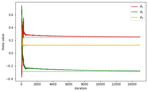
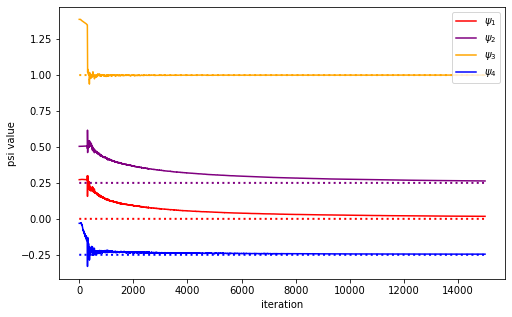
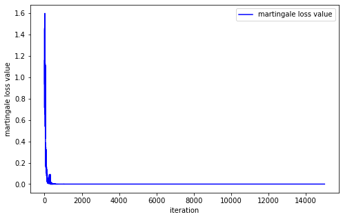
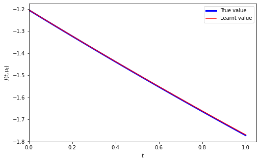
Figure 1: Convergence of value function and q function for Algorithm 1. Paths of learnt parameters for value function (top left) and paths of learnt parameters for q function (top right) vs optimal parameters shown in the dashed line. The change of the martingale loss value over iterations (bottom left) and the learnt value vs the optimal one (bottom right) along a trajectory $(\bar{\mu}_{t_{k}},{\rm Var}(\mu)_{t_{k}})_{k}$ with $\bar{\mu}_{0}=0$ and ${\rm Var}(\mu)_{0}=1$ controlled by the learnt policy and by the optimal policy.

Table 1:

	$\theta_{1}$	$\theta_{2}$	$\theta_{3}$	$\psi_{1}$	$\psi_{2}$	$\psi_{3}$	$\psi_{4}$
true value	0.25	-0.286	0.125	0	0.25	1	-0.25
learnt by Algorithm 1	0.2551	-0.278	0.125	0.0175	0.263	0.9999	-0.246

6.2 Mean-Field Optimal Consumption Problem

We consider the mean-field R$\&$D project process that is governed by the McKean-Vlasov SDE

$$dX_{s}^{\bm{\pi}}=a_{s}b\mathbb{E}[X_{s}^{\bm{\pi}}]ds+\sigma\mathbb{E}[X_{s}^{\bm{\pi}}]dW_{s}-c_{s}ds,(a_{s},c_{s})\sim{\bm{\pi}}(\cdot|s,X_{s}^{\bm{\pi}},\mathbb{P}_{X^{\bm{\pi}}_{s}}),\;X_{t}=x>0,$$ (6.5)

with $b>0$ and $\sigma>0$. Here, $a_{s}$ is the drift control of the R$\&$D investment and $c_{s}>0$ is the consumption rate. Let us consider the problem of expected utility on consumption subjecting to the quadratic cost of control in the following form that

$$J(t,\mu;\{a_{s}\}_{s\geq t},\{c_{s}\}_{s\geq t})=\mathbb{E}\biggl{[}\int_{t}^{T}e^{-\beta(s-t)}U(c_{s})ds-\int_{t}^{T}e^{-\beta(s-t)}a_{s}^{2}ds\biggl{]}$$

with the logrithmic utility function $U(x)=\log x$. The exploratory control-consumption performance after the entropy regularizer is defined by

$$J(t,\mu;{\bm{\pi}}) =\mathbb{E}\biggl{[}\int_{t}^{T}\int_{\mathbb{R}\times\mathbb{R}_{+}}\biggl{\{}e^{-\beta(s-t)}\Big{(}U(c)-e^{-\beta(s-t)}a^{2}-\gamma\log{\bm{\pi}}(a,c|s,X_{s}^{\bm{\pi}},\mathbb{P}_{X^{\bm{\pi}}_{s}})\Big{)}\biggl{\}}{\bm{\pi}}(a,c|s,X_{s}^{\bm{\pi}},\mathbb{P}_{X^{\bm{\pi}}_{s}})dadcds\biggl{]}.$$

The Hamiltonian operator is given by

$$H(t,x,\mu,a,c,p,q) =(b\bar{\mu}a-c)p+\frac{1}{2}\bar{\mu}^{2}\sigma^{2}q+\log(c)-a^{2}.$$

It then follows that

$$\int_{\mathbb{R}\times\mathbb{R}_{+}}\exp\Big{(}\frac{1}{\gamma}H(t,x,\mu,a,c,p,q)\Big{)}dadc$$

$$= \exp\Big{(}\frac{1}{2\gamma}\bar{\mu}^{2}\sigma^{2}q\Big{)}\int_{\mathbb{R}}\exp\Big{(}\frac{1}{\gamma}abp\bar{\mu}-\frac{1}{\gamma}a^{2}\Big{)}da\int_{\mathbb{R}_{+}}\exp\Big{(}\frac{1}{\gamma}\log(c)-\frac{p}{\gamma}c\Big{)}dc$$

$$= \sqrt{\gamma\pi}\exp\Big{(}\frac{1}{2\gamma}\bar{\mu}^{2}\sigma^{2}q\Big{)}\exp\left(\frac{b^{2}p^{2}\bar{\mu}^{2}}{4\gamma}\right)\frac{\Gamma(1+1/\gamma)}{(\frac{p}{\gamma})^{1+1/\gamma}}$$

With the terminal condition $J^{*}(T,\mu)=0$, we can write the exploratory HJB equation by

$$\frac{\partial J^{*}}{\partial t}(t,\mu)-\beta J^{*}(t,\mu)+\gamma\int_{\mathbb{R}_{+}}\log\int_{\mathbb{R}\times\mathbb{R}_{+}}\exp\Big{(}\frac{1}{\gamma}H(t,v,\mu,a,c,\partial_{\mu}J^{*}(t,\mu)(v),\partial_{v}\partial_{\mu}J^{*}(t,\mu)(v)\Big{)}dadc\mu(dv)$$

$$= \frac{\partial J^{*}}{\partial t}(t,\mu)-\beta J^{*}(t,\mu)+\frac{1}{2}\bar{\mu}^{2}\sigma^{2}\int_{\mathbb{R}_{+}}\partial_{v}\partial_{\mu}J^{*}(t,\mu)(v)\mu(dv)+\frac{1}{4}b^{2}\bar{\mu}^{2}\int_{\mathbb{R}_{+}}(\partial_{\mu}J^{*}(t,\mu)(v))^{2}\mu(dv)$$

$$\;+\frac{\gamma}{2}\log(\gamma\pi)+\gamma\log\Gamma(1+\frac{1}{\gamma})-(1+\gamma)\int_{\mathbb{R}_{+}}\log\Big{(}\frac{\partial_{\mu}J^{*}(t,\mu)(v)}{\gamma}\Big{)}\mu(dv).$$ (6.6)

Suppose that $J^{*}(t,\mu)$ satisfies the following form

$$J^{*}(t,\mu)=B(t)\log\bar{\mu}+D(t),$$

with the terminal conditions $B(T)=D(T)=0$. It holds that

$$\frac{\partial J^{*}(t,\mu)}{\partial t}=\dot{B}(t)\log\bar{\mu}+\dot{D}(t),\quad\partial_{\mu}J^{*}(t,\mu)(v)=B(t)\frac{1}{\bar{\mu}},\quad\partial_{v}\partial_{\mu}J^{*}(t,\mu)(v)=0.$$

Plugging these derivatives back into the exploratory HJB equation, we get that

$$\left({\dot{B}(t)}-\beta B(t)+1+\gamma\right)\log\bar{\mu}+{\dot{D}(t)}-\beta D(t)+\frac{1}{4}b^{2}B^{2}(t)+\frac{\gamma}{2}\log(\gamma\pi)+\gamma\log\Gamma(1+1/\gamma)$$

$$-(1+\gamma)\log\left(\frac{B(t)}{\gamma}\right)=0.$$

Together with $B(T)=0$, we first get that $B(t)=\frac{1+\gamma}{\beta}(1-e^{-\beta(T-t)})$ and

$${\dot{D}(t)}-\beta D(t)+\frac{1}{4}b^{2}\frac{(1+\gamma)^{2}}{\beta^{2}}(e^{-2\beta(T-t)}-2e^{-\beta(T-t)}+1)+K-(1+\gamma)\log(1-e^{-\beta(T-t)})=0,$$ (6.7)

where the constant $K:=\frac{\gamma}{2}\log(\gamma\pi)+\gamma\log\Gamma(1+1/\gamma)-(1+\gamma)\log\left(\frac{1+\gamma}{\beta\gamma}\right)$.

We can then obtain the explicit solution $D(t)$ of the ODE (6.7) with $D(T)=0$ as

$$D(t)= A_{1}e^{-2\beta(T-t)}+A_{2}e^{-\beta(T-t)}+A_{3}(1-e^{-\beta(T-t)})\log(1-e^{-\beta(T-t)})+A_{4}te^{-\beta(T-t)}+A_{5},$$

where

$$A_{1}:=-\frac{b^{2}(1+\gamma)^{2}}{4\beta^{3}},\quad A_{2}:=(1+\gamma)T-\frac{b^{2}(1+\gamma)^{2}}{2\beta^{2}}T-\frac{K}{\beta},$$

$$A_{3}:=-\frac{1+\gamma}{\beta},\quad A_{4}:=-(1+\gamma)+\frac{b^{2}(1+\gamma)^{2}}{2\beta^{2}},\quad A_{5}:=\frac{b^{2}(1+\gamma)^{2}}{4\beta^{3}}+\frac{K}{\beta}.$$

As a result, $q_{e}^{*}$ can be obtained explicitly

$$q_{e}^{*}(t,x,\mu,a,c)= \frac{\partial J^{*}(t,\mu)}{\partial t}-\beta J^{*}(t,\mu)+H(t,x,\mu,a,c,\partial_{\mu}J^{*}(t,\mu)(x),\partial_{v}\partial_{\mu}J^{*}(t,\mu)(x))$$

$$= -a^{2}+\frac{1+\gamma}{\beta}b(1-e^{-\beta(T-t)})a-\frac{1+\gamma}{\beta\bar{\mu}}(1-e^{-\beta(T-t)})c+\log c-(1+\gamma)\log\bar{\mu}$$

$$-\frac{b^{2}(1+\gamma)^{2}}{4\beta^{2}}(e^{-\beta(T-t)}-1)^{2}-K+(1+\gamma)\log(1-e^{-\beta(T-t)}).$$

Moreover, the separation form holds that ${\bm{\pi}}^{*}(a,c|t,x,\mu)={\bm{\pi}}_{1}^{*}(a|t,x,\mu){\bm{\pi}}_{2}^{*}(c|t,x,\mu)$, where ${\bm{\pi}}^{*}_{1}(a|t,x,\mu):=\mathcal{N}\Big{(}\frac{b(1+\gamma)}{2\beta}(1-e^{-\beta(T-t)}),\frac{\gamma}{2}\Big{)}$ and ${\bm{\pi}}_{2}^{*}(c|t,x,\mu):=\text{Gamma}(1+\frac{1}{\gamma},\frac{1+\gamma}{\gamma\beta\bar{\mu}}(1-e^{-\beta(T-t)}))$.

Therefore, when the model parameters are unknown, we can parameterize the optimal value function $J$, the optimal essential q-function $q_{e}$ and the optimal policy ${\bm{\pi}}^{*}$ respectively that

$$J^{\theta}(t,\mu)=\frac{1+\gamma}{\beta}(1-e^{-\beta(T-t)})\log\bar{\mu}+\theta_{1}e^{-2\beta(T-t)}+\theta_{2}e^{-\beta(T-t)}$$

$$-\frac{1+\gamma}{\beta}(1-e^{-\beta(T-t)})\log(1-e^{-\beta(T-t)})+\theta_{3}te^{-\beta(T-t)}+\theta_{4},$$

$$q_{e}^{\psi}(t,x,\mu,a,c)=-(1+\gamma)\log\bar{\mu}+\psi_{1}(1-e^{-\beta(T-t)})a-a^{2}+\psi_{2}(e^{-\beta(T-t)}-1)^{2}$$

$$-\frac{1+\gamma}{\beta\bar{\mu}}(1-e^{-\beta(T-t)})c+\log c-K+(1+\gamma)\log(1-e^{-\beta(T-t)})$$

$${\bm{\pi}}_{1}^{\psi}(a|t,x,\mu)=\mathcal{N}\Big{(}\frac{\psi_{1}}{2}(1-e^{-\beta(T-t)}),\frac{\gamma}{2}\Big{)},\ {\bm{\pi}}_{2}^{\psi}(c|t,x,\mu)=\text{Gamma}(1+\frac{1}{\gamma},\frac{1+\gamma}{\gamma\beta\bar{\mu}}(1-e^{-\beta(T-t)})).$$

The parameters are $\theta_{i}$, $i=1,\ldots,4$ and $\psi_{j}$, $j=1,2$. We also require $q_{2}^{\psi}$ to satisfy (5.1). In this case, $\psi_{2}=-\frac{\psi_{1}^{2}}{4}$.

The following simulator will be used in Algorithms 1-2 to generate sample trajectories.

Simulator  Under the stochastic policy ${\bm{h}}^{\tilde{\psi}}={\bm{h}}_{1}^{\tilde{\psi}}{\bm{h}}_{2}^{\tilde{\psi}}$, the dynamics (6.5) becomes

$$d\tilde{X}_{s}= b\mathbb{E}[\tilde{X}_{s}]\int_{\mathbb{R}}a{\bm{h}}_{1}^{\tilde{\psi}}(a|s,\tilde{X}_{s},\mathbb{P}_{\tilde{X}_{s}})dads-\int_{\mathbb{R}_{+}}c{\bm{h}}_{2}^{\tilde{\psi}}(c|s,\tilde{X}_{s},\mathbb{P}_{\tilde{X}_{s}})dcds+\sigma\mathbb{E}[X_{s}^{\bm{\pi}}]dW_{s}$$

$$= \frac{\tilde{\psi}_{1}b}{2}(1-e^{-\beta(T-s)})\mathbb{E}[\tilde{X}_{s}]ds-\frac{\beta}{1-e^{-\beta(T-s)}}\mathbb{E}[\tilde{X}_{s}]ds+\sigma\mathbb{E}[X_{s}^{\bm{\pi}}]dW_{s}.$$

By taking the expectation on both sides of the above SDE, we obtain that

$$d\mathbb{E}[\tilde{X}_{s}]=\frac{\tilde{\psi}_{1}b}{2}(1-e^{-\beta(T-s)})\mathbb{E}[\tilde{X}_{s}]ds-\frac{\beta}{1-e^{-\beta(T-s)}}\mathbb{E}[\tilde{X}_{s}]ds.$$

The Euler approximation of $\bar{\mu}_{t}=d\mathbb{E}[\tilde{X}_{s}]$ is

$$\log\bar{\mu}_{t_{k+1}}=\log\bar{\mu}_{t_{k}}+\Big{(}\frac{\tilde{\psi}_{1}b}{2}(1-e^{-\beta(T-s)})-\frac{\beta}{1-e^{-\beta(T-s)}}\Big{)}\Delta t.$$

The simulated reward is given by

$$\hat{r}_{t_{k}} =\int_{\mathbb{R}}\int_{\mathbb{R}_{+}}\log c{\bm{h}}_{2}^{\tilde{\psi}}(c|t_{k},x,\mathbb{P}_{\tilde{X}_{t_{k}}})dc\mathbb{P}_{\tilde{X}_{t_{k}}}(dx)-\int_{\mathbb{R}}\int_{\mathbb{R}}a^{2}{\bm{h}}_{1}^{\tilde{\psi}}(a|t_{k},x,\mathbb{P}_{\tilde{X}_{t_{k}}})da\mathbb{P}_{\tilde{X}_{t_{k}}}(dx)$$

$$=\frac{\Gamma^{\prime}(1+\frac{1}{\gamma})}{\Gamma(1+\frac{1}{\gamma})}-\log\big{(}\frac{1+\gamma}{\gamma\beta}(1-e^{-\beta(T-t)})\big{)}+\log\bar{\mu}+\frac{\tilde{\psi}_{1}^{2}}{4}(1-e^{-\beta(T-t)})^{2}+\frac{\gamma^{2}}{4}.$$

We first set coefficients of the simulator to $T=1,b=0.5,\sigma=0.5$. We next set the known parameters as: $\gamma=0.25$, $\beta=10$, the time step $\Delta t=0.05$, the number of episodes $N=15000$, the number of test policies $M=10$, the lower bound of uniform distribution $p(j)=0$, the upper bound of uniform distribution $q(j)=\frac{0.4}{j^{0.6}}$, the log mean $\log\mu_{0}^{m},1\leq m\leq M$ that is initialed to be 0, and the learning rates $(\alpha_{\theta},\alpha_{\psi})$ are given by

$$\alpha_{\theta}(j)=\left\{\begin{array}[]{lll}(0.005,0.003,0.003,0.001),&\mbox{if}\;j\leq 30,\\ (0.05,0.03,0.03,0.01),&\mbox{if}\;30<j\leq 900,\\ (0.01,0.01,0.01,0.001),&\mbox{if}\;900<j\leq 2000,\\ (0.002,0.002,0.001,0.001),&\mbox{if}\;2000<j<15000,\end{array}\right.$$

and

$$\alpha_{\psi}(j)=\left\{\begin{array}[]{lll}0.01,&\mbox{if}\;j\leq 30,\\ 0.005,&\mbox{if}\;30<j\leq 900,\\ 0.001,&\mbox{if}\;900<j\leq 15000.\end{array}\right.$$

Based on the offline q-learning Algorithm 1, we plot in Figure 2 the numerical results on the convergence of parameters $\theta$ and $\psi$ for the value function and q function, and also summarize the learnt parameters for the optimal value function and the optimal essential q-function $q_{e}$ in Table 2.

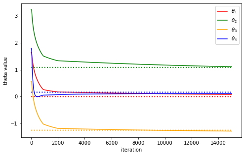
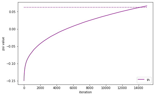
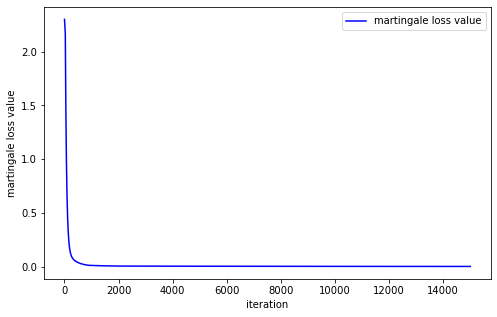
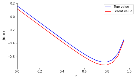
Figure 2: Convergence of value function and q function for Algorithm 1. Paths of learnt parameters for value function (top left) and path of learnt parameters for q function (top right) vs optimal parameters shown in the dashed line. The change of the martingale loss value over iterations (bottom left) and the learnt value vs the optimal one (bottom right) along a trajectory $(\log(\bar{\mu}_{t_{k}}))_{k}$ with $\log(\bar{\mu}_{0})=0$ controlled by the learnt policy and by the optimal policy.

Table 2:

	$\theta_{1}$	$\theta_{2}$	$\theta_{3}$	$\theta_{4}$	$\psi_{1}$
true value	-9.765 $\times 10^{-5}$	1.085	-1.248	0.163	0.0625
learnt by Algorithm 1	0.0796	1.107	-1.281	0.119	0.0667

7 Conclusion

This paper aims to lay the theoretical foundation of the continuous time q-learning for Mckean-Vlasov control problems, which can be viewed as the bridge between the discrete time Q-learning with the integrated Q-function for mean-field control problems studied in Gu et al. (2023) and the continuous time q-learning with the q-function for single agent’s control problems studied in Jia and Zhou (2022c). In our framework, two different q-functions are introduced for the purpose of learning, namely the integrated q-function $q$ that is defined as the first order derivative of the integrated Q-function with respect to time and the essential q-function $q_{e}$ that is used for policy improvement iterations. Comparing with two counterparts in Gu et al. (2023) and Jia and Zhou (2022c), we establish the weak martingale characterization of the value function and the integrated q-function through test polices in the neighbourhood of the target policy in a similar flavor of off-policy learning. To learn the essential q-function from the double integral representation, we propose the average-based loss function by searching test policies in the same form of the parameterized target policy but with randomized parameters. In two examples, one in the LQ control framework and one beyond the LQ control framework, we can illustrate the effectiveness of our q-learning algorithm.

Several interesting future extensions can be considered. Firstly, we may consider the controlled common noise in the McKean-Vlasov control problem, where the optimal policy no longer admits the explicit form as a Gibbs measure. Instead, we can provide the first order condition of the optimal policy using the linear derivative with respect to probability measures. It is an interesting open problem to investigate the correct form of the continuous time integrated q-function and the associated q-learning. Secondly, it will also be appealing to generalize the q-learning for continuous time graphon mean-field control problems for heterogenous interacting agents described by the graphon theory. It will be fascinating for both theories and algorithms if the proper martingale condition of the integrated q-function can be established for each type of agents. At last, we are also interested in extending our current results on q-learning to other mean-field systems such as learning mean-field games and mean-field games of controls.

Acknowledgement: X. Wei is supported by National Natural Science Foundation of China grant under no.12201343. X. Yu is supported by the Hong Kong Polytechnic University research grant under no. P0045654.

References

- Angiuli et al. (2022) A. Angiuli, J. P. Fouque and M. Laurière. (2022). Unified reinforcement Q-learning for mean field game and control problems. Mathematics of Control, Signals, and Systems, 34(2), 217-271.
- Carmona and Delarue (2018a) R. Carmona and F. Delarue (2018a): Probabilistic Theory of Mean Field Games with Applications, Vol I. Springer.
- Carmona and Delarue (2018b) R. Carmona and F. Delarue (2018b): Probabilistic Theory of Mean Field Games with Applications, Vol II. Springer.
- Carmona et al. (2015) R. Carmona, J. P. Fouque and L. H. Sun (2015): Mean field games and systemic risk. Communications in Mathematical Sciences, 13(4):911-933.
- Cosso et al. (2020) A. Cosso, F Gozzi, I. Kharroubi, H. Pham and M. Rosestolato (2020): Optimal control of path-dependent McKean-Vlasov SDEs in infinite dimension. Preprint, arXiv:2012.14772.
- Doya (2020) K. Doya (2020). Reinforcement learning in continuous time and space. Neural Computation, 12(1):219–245.
- Gu et al. (2023) H. Gu, X. Guo, X. Wei and R. Xu (2023): Dynamic programming principles for mean-field controls with learning. Operations Research, forthcoming, DOI:10.1287/opre.2022.2395.
- Guo et al. (2022) X. Guo, R. Xu and T. Zariphopoulou (2022): Entropy regularization for mean field games with learning. Mathematics of Operations Research, 47(4), 3239-3260.
- Frikha et al. (2023) N. Frikha, M. Germain, M. Laurière, H. Pham. and X. Song (2023). Actor-Critic learning for mean-field control in continuous time. arXiv preprint arXiv:2303.06993.
- Jia and Zhou (2022a) Y. Jia and X. Y. Zhou (2022a): Policy gradient and actor-critic learning in continuous time and space: Theory and algorithms. Journal of Machine Learning Research. 23, 1-50.
- Jia and Zhou (2022b) Y. Jia and X. Y. Zhou (2022b): Policy evaluation and temporal-difference learning in continuous time and space: A martingale approach. Journal of Machine Learning Research. 23, 1-55.
- Jia and Zhou (2022c) Y. Jia and X. Y. Zhou (2022c): q-learning in continuous time. Forthcoming in Journal of Machine Learning Research.
- Lacker (2017) D. Lacker (2017): Limit theory for controlled McKean-Vlasov dynamics. SIAM Journal on Control and Optimization, 55(3):1641-1672.
- Li et al. (2023) N. Li, X. Li and Z. Xu (2023): Policy iteration reinforcement learning method for continuous time mean field linear-quadratic optimal problem. Preprint, arXiv:2305.00424.
- Lions (2006) P.-L. Lions (2006): Cours au collège de france: Théorie des jeux à champ moyens. Audio Conference.
- Motte and Pham (2022) M. Motte and H. Pham (2022): Mean-field Markov decision processes with common noise and open-loop controls. The Annals of Applied Probability, 32(2):1421-1458.
- Schulman et al. (2017) J. Schulman, X. Chen and P. Abbeel (2017): Equivalence between policy gradients and soft Q-learning. Preprint arXiv:1704.06440.
- Sutton and Barto (2018) R. S. Sutton and A. G. Barto (2018): Reinforcement learning: An introduction. MIT press.
- Wang et al. (2020) H. Wang, T. Zariphopoulou and X. Y. Zhou (2020): Reinforcement learning in continuous time and space: A stochastic control approach. Journal of Machine Learning Research, 21(1):8145-8178.