Neural directional distance field object representation for uni-directional path-traced rendering

Abstract

Faster rendering of synthetic images is a core problem in the field of computer graphics. Rendering algorithms, such as path-tracing is dependent on parameters like size of the image, number of light bounces, number of samples per pixel, all of which, are fixed if one wants to obtain a image of a desired quality. It is also dependent on the size and complexity of the scene being rendered. One of the largest bottleneck in rendering, particularly when the scene is very large, is querying for objects in the path of a given ray in the scene. By changing the data type that represents the objects in the scene, one may reduce render time, however, a different representation of a scene requires the modification of the rendering algorithm. In this paper, (a) we introduce directed distance field, as a functional representation of a object; (b) how the directed distance functions, when stored as a neural network, be optimized and; (c) how such an object can be rendered with a modified path-tracing algorithm.

I Introduction

Path tracing is used for faithfully reproducing photo-realistic images from a mathematical description of a 3D scene. However, path tracing algorithm has very high resource requirements and it takes a long time to render a image. As the demand for real time rendering increases, the field has seen a lot of interest in recent years, and many techniques have been proposed for making the rendering faster, by adding hardware resources like more powerful GPUs, vectorizing computation on hardware[1] and using learning algorithms like the deep learning supersampling[2].

Nevertheless, the core path tracing algorithm has seen little change towards faster rendering. One bottleneck in path tracing algorithm occurs when the algorithm computes ray-triangle intersection against every triangle in the scene. A linear search for the nearest triangle in the scene becomes extremely slow. Use of data structures like bounding volume hierarchies (BVH), Octrees and Kd-trees [3] has helped in reducing it to log-linear time. In this paper, we propose a data structure that we call the directed distance function that theoretically takes a constant time to compute the nearest ray-triangle intersection, albeit with a preprocessing time for building the data structure.

The directed distance field can be used to represent individual objects as well as entire scene. Directed distance fields are dense fields on five-dimensional space and hence representing them is also not trivial since a discretization will consume $O(n^{5})$ space. The field can be stored as a pure function, which although extremely fast, it hard to build (for artists). In this paper, we explore neural networks as a universal function estimator to represent the field.

To estimate the field with neural networks, we need training data. The field around the object is complex which necessitates a systematic sampling technique for building the dataset to train on. Otherwise the network fails to learn the distance field of the object. We introduce sampling technique to build the dataset and observe that it performs better than sampling techniques used in similar works.

Rendering algorithms are generally tied to the underlying scene representations. For example, sphere tracing for signed distance fields and ray-triangle intersections for polyhedral mesh. Hence, we propose a modification to the path tracing algorithm to render a directed distance field. We modify the path tracing algorithm to use this data structure.

In this paper, our contribution are as follows.

1. We analyze directed distance function as a alternative representation of object for path-trace rendering.

2. We provide modification of the path-tracing rendering algorithm to be able to render DDFs, which are represented as neural networks.

3. We provide a informative sampling techniques to build datasets to optimize the above given neural network.

II Related Works

The rendering algorithm depends largely on the the underlying data structure that represents the scene. Therefore, we discuss different representations in this section.

Explicit representation. In explicit scene representation, the geometry is defined in terms of the explicit location of the objects and its properties in the scene. Such explicit representation include point clouds, meshes, voxels which include the position of the vertices and their color. The rendering algorithm makes direct queries about these properties in the scene, while rendering. Since the explicit representation is compact, easy to represent and reason with while also providing easier ways to model the scene (for artists.) However, their topology is not easily handled, for example, performing boolean operation like union, intersection in constructive solid geometry, or in computer vision, for learning algorithms that reconstruct geometry from images becomes hard and, sometimes impossible.

Implicit representation. The geometry can be defined without explicitly defining the location and color of objects in the scene, and using the functions instead. The most popular of such implicit representation is the signed distance function. Signed distance functions (sometimes, just distance field or SDFs), is a field over the 3D space $\mathbb{R}^{3}$, where every point in the field is defined as the distance to the nearest surface. The sphere tracing algorithm[4] is used to render SDF. However, storing SDFs as discretized values comes with a huge space cost and hence have seen very limited use or are manually crafted by artists with mathematical functions. It’s resurgence in recent years is due to learning algorithms that can represent arbitrary functions and can be learned. The zero level set of a signed distance function represents the surface.

Other implicit function representations that are popular in learning algorithms are radiance fields[5], that are like SDF but instead of distances, the field values stores the color and density (or opacity) of the point. They are particularly suited for volumetric rendering. If, instead the points only represent whether it is inside or outside a surface, the field is occupancy function. These functions are learned with universal function approximators like neural networks[6] and can be converted into explicit representation by marching cubes[7] algorithm.

Directional distance function. Signed distance functions with directional component has been used in prior works[8, 9, 10, 11, 12] for shape representation and reconstruction using learning algorithms. Truncated Signed Directional Distance function[10] have been used for pose estimation. The geometric properties of DDFs, and differentiable rendering of DDFs by using a probabilistic directional distance field with $C^{1}$ consistency for are discussed in [8]. However, they are ray-traced rendered instead of path-traced. Although this technique is suitable for reconstruction, it cannot be used for multiple bounce path-traced physically based rendering. Directional distance function are used for representation and reconstruction of shapes that are to be optimized for rendering with learning algorithms like neural networks with single images[8, 11], with ground truth meshes[8, 9] and with multiple images and their depth fields[11].

III Background

In this section, we introduce the directed distance function, it’s mathematical properties and the rendering pipeline, as required in the later sections.

III-A Directional signed distance functions

Let $S$ be the surface of a 3D object which lies entirely within the bounded box $B\subset\mathbb{R}^{3}$. A directional distance field (DDF) $\phi:B\times\mathbb{R}^{2}\to\mathbb{R}^{+}$ takes point, $x\in B$ and direction, $\theta\in\mathbb{R}^{2}$ (henceforth viewing direction) and returns the minimum distance $d$, from the point $x$, to the surface $S$, in the direction $\theta$. A binary visibility function $\xi(x,\theta)=\mathbbm{1}_{S}(x,\theta)$ returns 1 if the ray $x$ in direction $\theta$ intersects the surface $S$. The oriented point $(x,\theta)$ is said to be visible if $\mathbbm{1}_{S}(x,\theta)$ returns 1. In the following paragraphs, we present some geometric properties of DDF (proof of which maybe found at [8, 12]).

For a given point, $x$, any viewing angle, $\theta$ can be represented in two degree of freedom, with azimuthal $\theta_{0}$, and polar $\theta_{1}$ angles, for example. When specified with those angles, moving $t$ distance from $x$ in $\theta$ direction is,

$$x^{\prime}=x+t\begin{bmatrix}\cos(\theta_{0})\sin(\theta_{1})&\sin(\theta_{0})\sin(\theta_{1})&\cos(\theta_{1})\end{bmatrix}^{T}$$ (1)

We abuse the notation and write $x+t\theta$ to refer to the point at $t$ distance from $x$ in the viewing direction, $\theta$, as this way is popularly used in ray marching computations. The actual computation is implementation-specific.

Directed Eikonal Equation. For any visible oriented point $(p,\theta)$, the following holds,

$$\partial_{x}\phi(x,\theta)\cdot\theta=-1$$ (2)

In the viewing direction, for every marching step the DDF value decreases by the step size, i.e, the DDF, $\phi(x,\theta)-\phi(x+t\theta,\theta)=t$, which follows that the maximum rate of change in $\phi$ occurs in the direction opposite to the viewing direction.

Surface normal. The point on the surface $S$ is given as, $q(x,\theta)=\phi(x,\theta)\theta+x\in S$. The normal at the given surface is given by,

$$n(x,\theta)=\frac{\kappa\partial_{x}\phi(x,\theta)^{T}}{\lVert\partial_{x}\phi(x,\theta)\rVert_{2}}$$ (3)

where $\kappa$ is chosen from $\{-1,1\}$ such that $n^{T}\theta<0$.

Gradient consistency. From any visible oriented point $(x,\theta)$, a infinitesimal change in the viewing direction, $\delta\theta$ effectively pushes the position $x$ in the direction, $\theta$, i.e,

$$\partial_{\theta}\phi(x,\theta)=\phi(x,\theta)\partial_{x}\phi(x,\theta)\delta\theta$$ (4)

where $\partial\theta=\omega\times\theta$. This relates the gradient of $\phi$ with a rotational perturbation $\partial\theta$ with respect to both position and direction.

Unsigned distance field. The distance field (like signed distance function, except that the field is not negative inside the surface), can be recovered from the DDF by computing the minimum of DDF against all the direction for any given point $x$,

$$\text{UDF}(x)=\min_{\theta}\phi(x,\theta)$$ (5)

The UDF (unlike DDF) has no discontinuities.

Locally differentiable For any visible oriented point $(x,\theta)$, the geometry of 2D manifold $S$ near $q$ is completely characterized by $\phi(x,\theta)$ and it’s derivatives. This allows us to recover the surface properties like normals and curvature from the DDF only.

The above mentioned properties will be used to modify the path tracing algorithm to use DDF to render images. The reader may refer to [8, 12] for a more general and detailed treatment of DDF.

IV Methodology

Figure 1: The 2D cross-section of a scene: With respect to the rendering equation demonstrates the path the light takes at multiple after bounces in the and the radiance computation over the hemisphere, $\Omega$.

IV-A Object representation

Neural network. When the DDF is stored as a neural network, the DDF is learned either from a set of multiple images[13] or ground truth scene. We will only discuss ground truth mesh in this work. Consider a neural network, $\text{MLP}_{w}:(\mathbb{R}^{3},\mathbb{R}^{2})\to\mathbb{R}$ that takes a oriented point $(x,\theta)$ and returns the DDF field value. Given a triangle mesh scene, the training dataset consists of sampling points from bounding box. After the weights $w$ are optimized, the $\text{MLP}_{w}$ can be used for rendering the scene.

For invisible oriented points, the field value $\phi(x,\theta)$ is set to $\infty$, however this causes problem in optimizing the network for the object. Therefore a squishing function maybe used for learning the field value, with the loss function,

$$L_{w}=\sigma(y)-\sigma(\tilde{y})$$ (6)

where, $y=\phi_{\text{gt}}(x,\theta)$ is the ground truth DDF value, $\tilde{y}=\text{MLP}_{w}(x,\theta)$ is the network representation of the object and the squish function[12] $\sigma(x)$ is a strictly increasing function that approaches a finite value as input $x$, approaches $\infty$, like tanh$(x)$ or erf$(x)$.

IV-B Surface normal computation

The normal is required at each intersection of the ray with the scene for shading. The normal of a directed distance field can be computed using Eq. 3 by exploiting the fact that the distance function is locally differentiable. As the DDF is stored as neural network, the normals are trivial to compute with automatic differentiation,

$$\partial_{x}\phi(x,\theta)=\partial_{x}\text{MLP}_{w}(x,\theta)$$ (7)

taking care to find the derivative with respect to the input point $x$, rather than the weights $w$ as done in general backward pass. In PyTorch, the relevant code will be,

⬇

ddf = MLP(position, direction)

ddf.backward()

normal = position.grad

The $\kappa$ is assigned to make the normal point outward, using the dot product, between the normal and viewing direction such that, $n^{T}\theta<0$.

V Dataset, network architecture, and renderer

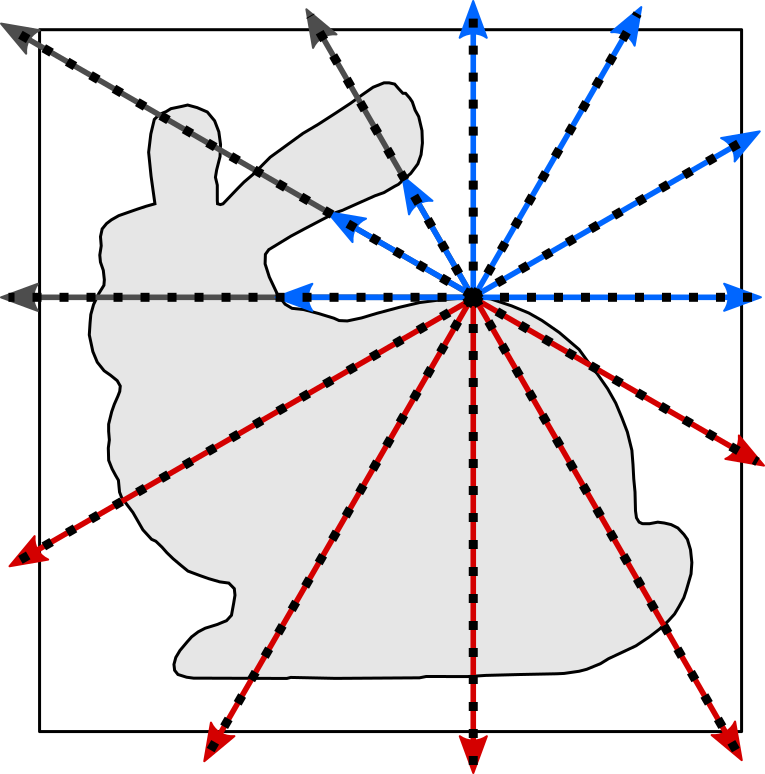
(a)

(b)

Figure 2: (a) Sampling strategy: the object, bunny rabbit is shown in gray in the bounding box. The points sampled from the ray shown in red and gray are rejected, while the points on ray in blue is accepted into the training data. (b) collecting data-points on rays from the surface: at point, $q=p+\theta{}t$, the distance to the surface in the direction $-\theta$ is $t$, and in the direction $\theta$, if it doesn’t hit any other face, the field value is infinite.

V-A Neural network architecture and training

The neural network is written in Pytorch. The network is a fully connected network with 8 weight-normalized hidden layers of width 512 followed by ReLU activation and dropout (with probability, $p=0.5$). The network was optimized with Adam optimizer, with learning rate $10^{-7}$ over the clamp error loss defined as,

$$L =\lvert\text{clamp}(y,\delta)-\text{clamp}(\tilde{y},\delta)\rvert$$ (8)

where $\text{clamp}(x,\delta):=\min(\delta,\max(-\delta,x))$ is the squishing function with hyperparameter $\delta$ to control the distance from the surface over which we optimize the network over. Larger values of $\delta$ helps in ray tracing the object from larger distances, while the smaller values helps concentrate the network capacity on surface details. This is a trade-off between surface details and draw distance for ray-tracing.

For training the network, we generate the training data by sampling points from the bounding box, $B$. Uniform random sampling the points and viewing directions trains the network poorly because many oriented points have infinite values and hence, do not contribute to the shape estimation. Therefore, we have used a more informative sampling over the surface to learn from, as described in the next section.

V-B Dataset preparation

The directed distance field changes rapidly around the object it represents, while also being in five-dimension. Therefore without a dense sampling of the field values around the point, the neural network cannot optimize the object shape. We start from the ground truth triangle mesh containing vertices and faces. We use three hyperparameters for sampling the training data points, face samples $s_{\text{fc}}$, direction samples $s_{\text{dr}},$ and marching samples $s_{\text{p}}$.

To sample a point $q$, from a face with vertices $\{p_{0},p_{1},p_{2}\}$, we first sample two real values from the uniform distribution $U$, and use the barycentric co-ordinates to get points on the face.

$$\begin{split}S_{\text{fc}}=\{&(1-a-b)p_{0}+ap_{1}+bp_{2}:\\ &a,b\sim U[0,1]\},\;|S_{\text{fc}}|=s_{\text{fc}}\end{split}$$ (9)

And for sampling directions, we sample from a uniform distribution and convert it to polar angle $\theta_{0}$, and azimuthal angle $\theta_{1}$.

$$\begin{split}S_{\text{dr}}=\{&\theta_{0}=a\pi,\;\theta_{1}=2b\pi:\\ &a,b\sim U[0,1]\},\;|S_{\text{dr}}|=s_{\text{dr}}\end{split}$$ (10)

For each points on the face $p\in S_{\text{fc}}$, and direction $\theta\in S_{\text{dr}}$, we march the ray in steps of $t$ and collect the field values into the training dataset $D$ (Figure 2),

$$D\leftarrow(p+t\theta,-\theta;t)\cup D,\quad\text{for}\;t>0$$ (11)

except for two conditions: (a) if the ray marches into the mesh, where by definition the field value is not defined (red rays) or, (b) the ray hits another part of the mesh, (gray rays, in Fig.2). In either case, we have used odd-even rule to determine whether the direction we are sampling is inside or outside the mesh, using the fact that when is outside the bounding box of the mesh, the ray is always also outside the mesh. In case, the ray never enters the mesh, we also collect the following values too,

$$D\leftarrow(p+t\theta,\theta;\infty)\cup D,\quad\text{for}\;t>0$$ (12)

$$D\leftarrow(p+t\theta,\theta\pm\pi/2;\infty)\cup D,\quad\text{for}\;t>0$$ (13)

We sample according to Eq. (13) only when the angles perpendicular to $\theta$ do not hit any face. We ignore when it hits the face because, in that case, the rays sampled from the face it hits will cover field value at the point.

VI Result and evaluation

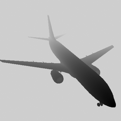
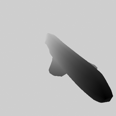
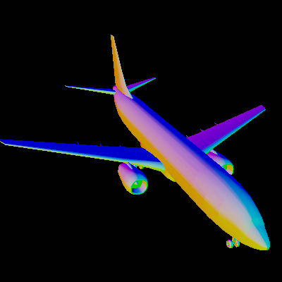
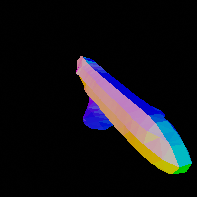
(airplane)

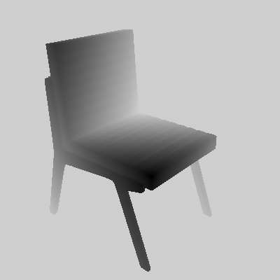
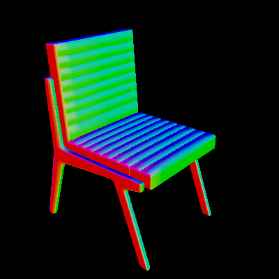
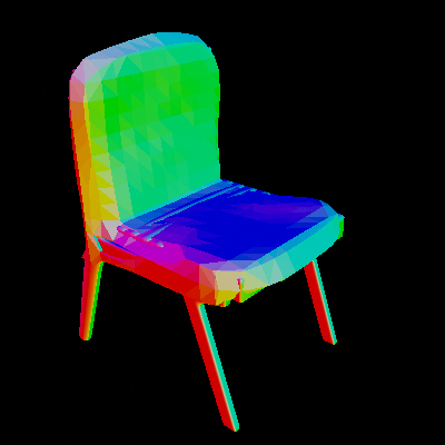
(chair)

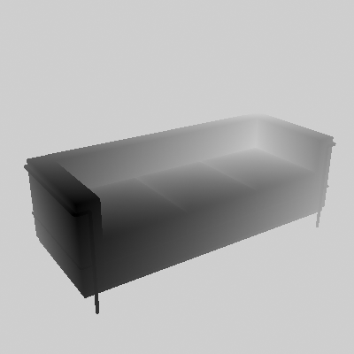
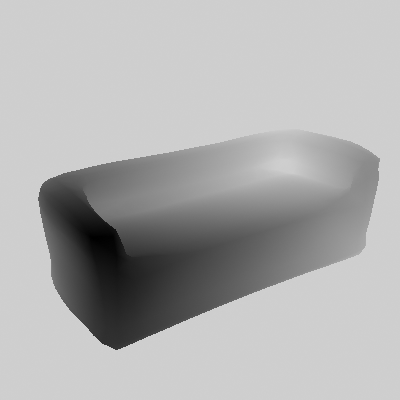
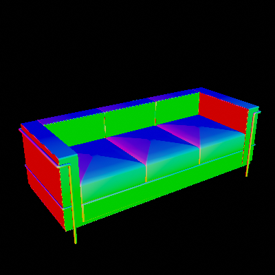
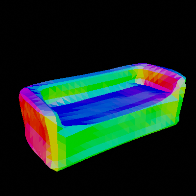
(couch)

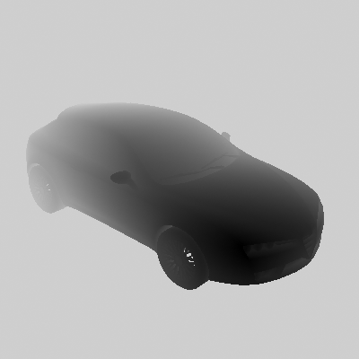
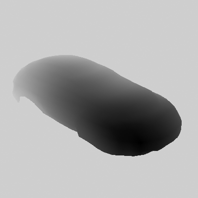
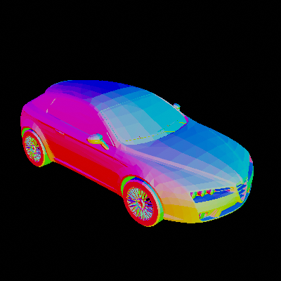
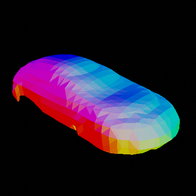
(car)

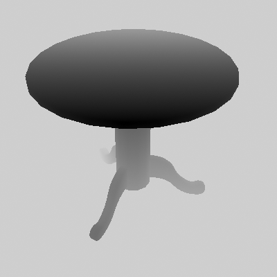
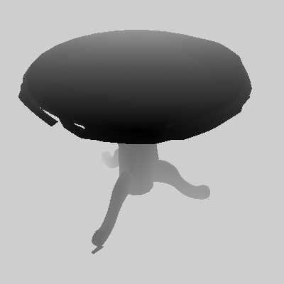
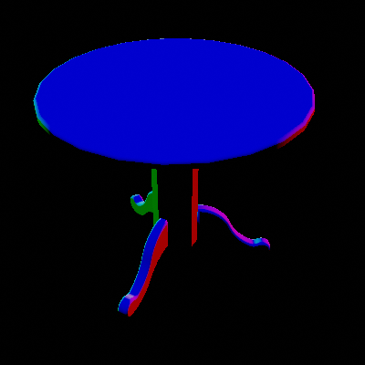
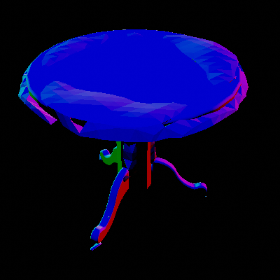
(table)

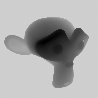
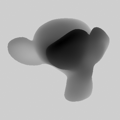
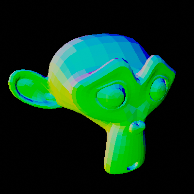
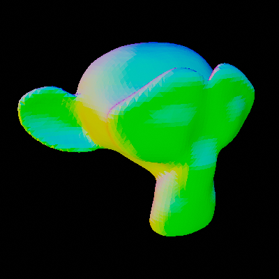
(suzanne)

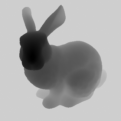
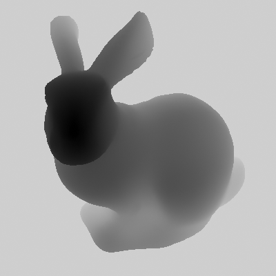
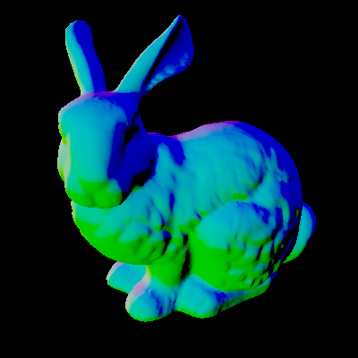
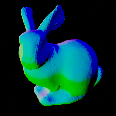
(bunny)

Figure 3: Comparison of the predicted in different categories from top to bottom: ground truth field values, predicted field values, ground truth normal and predicted normal for different categories: airplane, chair, couch, car, table, suzanne and bunny. (Note, that this is in Z-up co-ordinate system)

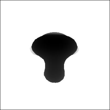
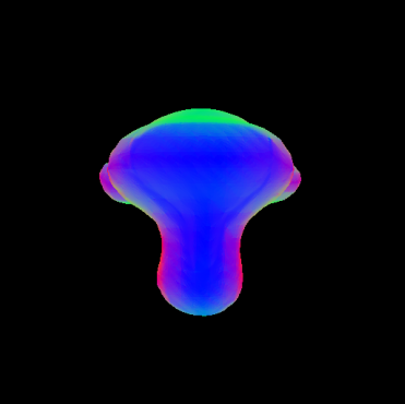
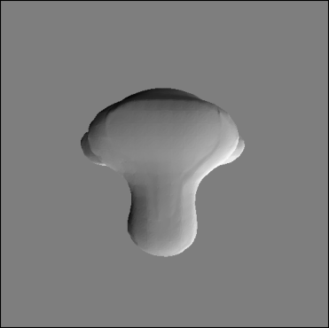
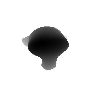
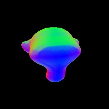
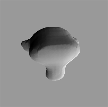
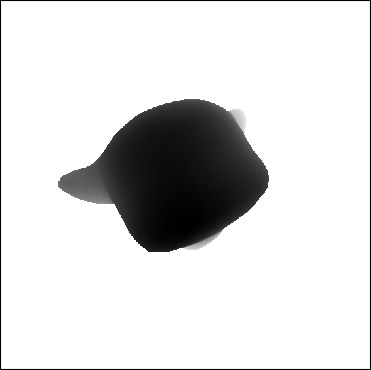
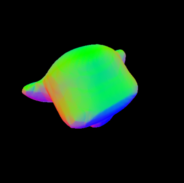
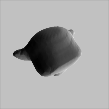
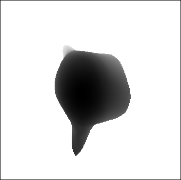
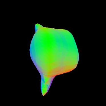
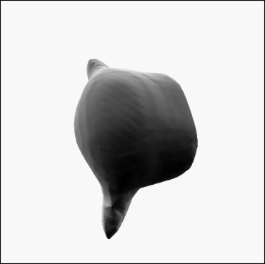
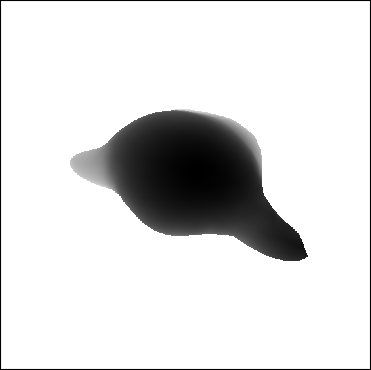
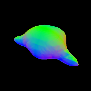
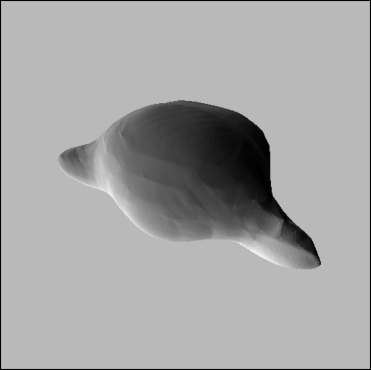
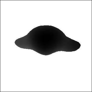
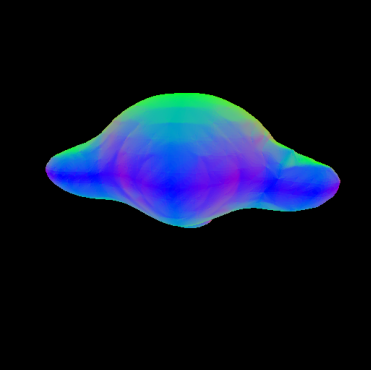
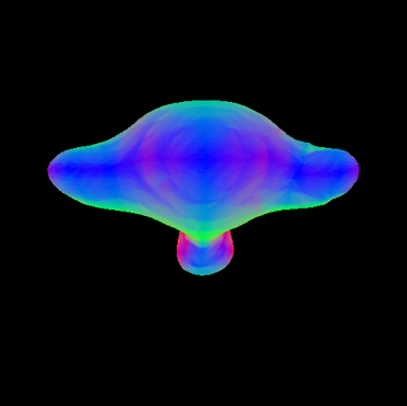
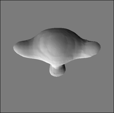
Figure 4: The output of our renderer for $t$-values (top), normal map (middle) and ray-traced (bottom) rendering from a sample different azimuthal and polar angles.

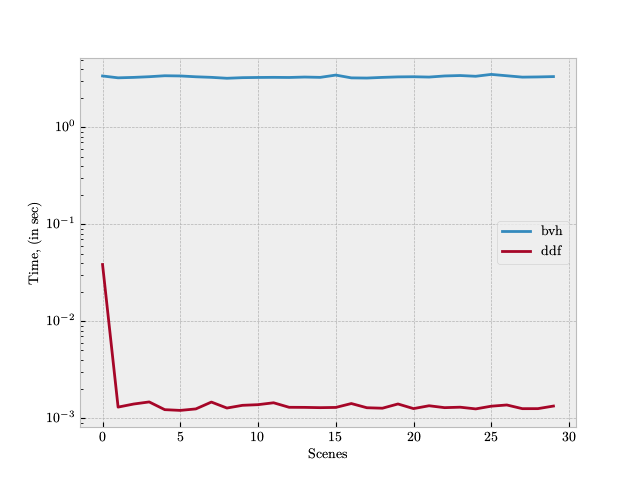
Figure 5: The time taken to render images, by DDF and by BVH. Rendering took more time the first time around because, the data need to be copied to the GPU and cached. After that, the neural network is cached on the GPU, the subsequent render time decreases. Note that the y-axes is in log-scale.

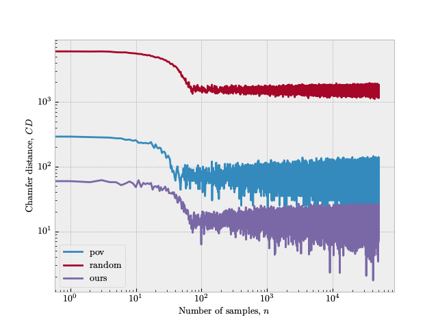
Figure 6: The chamfer distance $CD$ of the learned DDF field, against the number of samples. Note that this is a log-log plot of different sampling techniques: random, pov and ours.

TABLE I: Experimental comparison of shape reconstruction of DeepSDF, DeepDDF and ours with chamfer distance (in multiple of $10^{3}$) against the ground truth (lower is better).

Object	DIST[14]	DeepSDF[15]	DeepDDF[13]	Ours
Chair	0.560	0.512	0.533	0.519
Car	0.521	0.475	0.430	0.681
Table	0.738	0.655	0.611	0.701
Couch	0.731	0.692	0.693	0.665
Airplane	0.831	0.792	0.735	0.951
Bunny	–	–	–	0.589
Suzanne	–	–	–	0.603

VI-A Ablation study

We evaluate our methodology against different hyperparameter by the following metrics between the reconstructed mesh and the ground truth values: (a) chamfer distance,

$$\begin{split}\text{CD}(P_{1},P_{2})=&\dfrac{w_{1}}{|P_{1}|}\sum\limits_{p_{1i}\in P_{1}}\min\limits_{p_{2j}\in P_{2}}(||p_{1i}-p_{2j}||_{2}^{2})+\\ &\dfrac{w_{2}}{|P_{2}|}\sum\limits_{p_{2j}\in P_{2}}\min\limits_{p_{1i}\in P_{1}}(||p_{2j}-p_{1i}||_{2}^{2})\end{split}$$ (14)

(b) the f-score, and (c) the sided distance,

$$\text{SD}(p_{1i},P_{2})=\min\limits_{p_{2j}\in{P_{2}}}(||p_{1i}-p_{2j}||_{2}^{2})$$ (15)

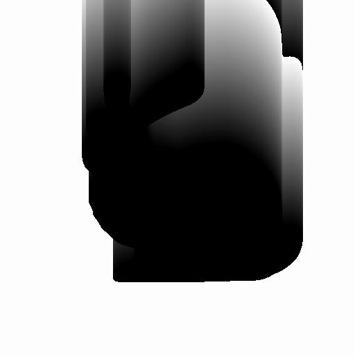
0^∘

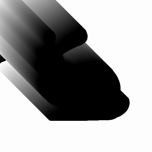
45^∘

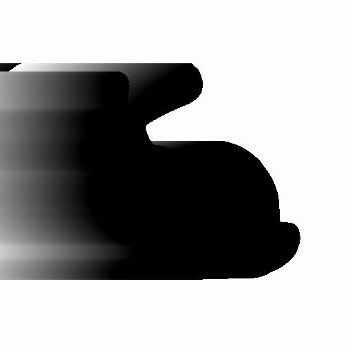
90^∘

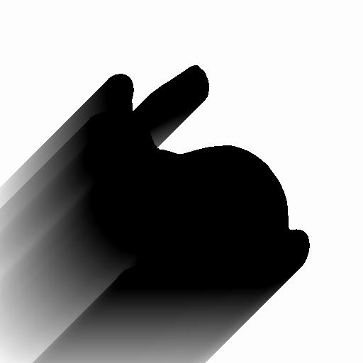
135^∘

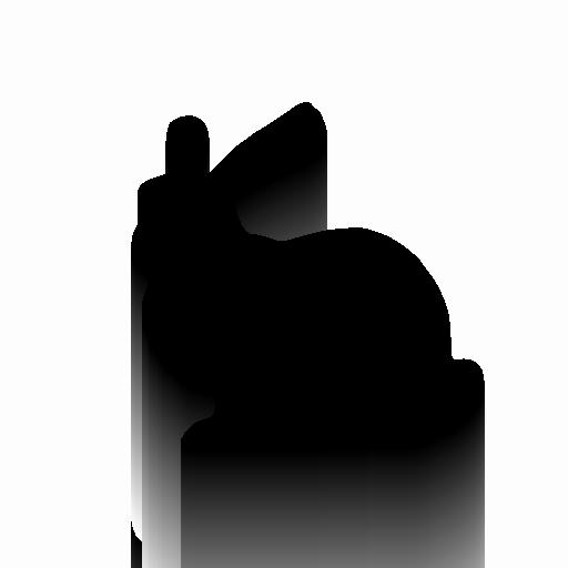
180^∘

225^∘

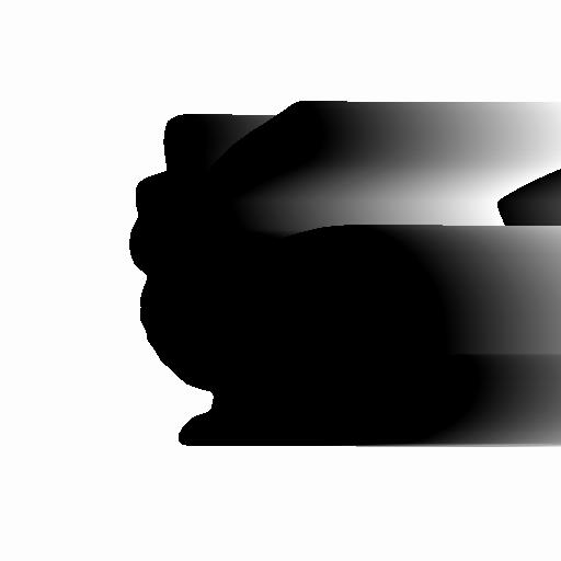
270^∘

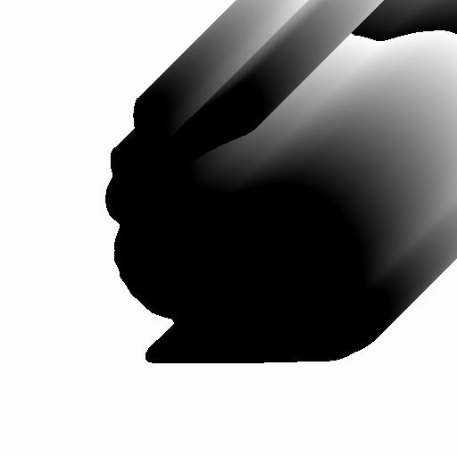
315^∘

Figure 7: Shows the field values for a given cross-section of bunny rabbit for for different polar angles. The grayscale intensity denotes the $t$-value with black as zero.

All of these metrics are computed on sets of points (or point cloud). The DDF was converted into UDF (Eq. 5), which in turn was converted into a triangle mesh using the marching cubes algorithm from (Sci-kit image library[16]) and computed using the Kaolin library[17]. Table. II show the hyperparameters $s_{\text{fc}}$, $s_{\text{dr}},$ and $s_{\text{p}}$ against the above metrics where we observer that increasing the samples per face $s_{\text{fc}}$ has less effect, than increasing the $s_{\text{p}}$ and lesser still for $s_{\text{dr}}$.

TABLE II: Hyperparameter sensitivity: $s_{\text{fc}}$, $s_{\text{dr}},$ and $s_{\text{p}}$ against CD (in multiple $10^{3}$, lower is better).

n	$s_{\text{fc}}$	$s_{\text{dr}}$	$s_{\text{p}}$
10	0.714	0.944	0.832
20	0.829	0.723	0.019
30	0.694	0.564	0.005

VI-B Results

For code and instruction on how to reproduce the results of this paper, one may visit the following URL, www.github.com/smlab-niser/23ddf. We evaluate the above theories on a set of following triangle mesh from the ShapeNet[18] dataset: airplane, car, chair, couch and table. We have also tested the result on two standard test meshes: Standford bunny and Blender Suzanne monkey. All the training and experimentation was done on a Ryzen Threadripper 3970X CPU with RTX 3090 GPU. Building the dataset took 5 hours for each mesh, while the training the neural network took 20 hours for 10,000 iteration. The reconstructed mesh is given in Fig. 3. We have compared the chamfer distance against the similar work in Table. I. Although, our methodology performs closer to similar works, it performs as good with much less number of iterations and while also allowing for faster rendering.

Fig. 6 shows the chamfer distance, distance between the ground truth ShapeNet and the reconstructed mesh for different sampling techniques. For random, points and directions were picked from the bounding box at random, a ray was shot in the direction and the $t$-value was stored. For pov (point-of-view) sampling, we set up cameras pointed at the mesh center around the mesh, by uniformly spacing 10 cameras around azimuthal and 5 cameras around polar angles, for a total of 50 cameras. For every pixel in the camera film, we shot rays and calculated the $t$ values. We observe that out sampling works better than the other techniques.

We demonstrate ray-tracing with our renderer for depth ($t$-value) and normal values using DDF and without DDF that uses BVH to search for hit point and compare the time taken Fig. (5) and sample renders Fig. (4) for bunny. We observe that our renderer works very much faster with DDF than without.

VII Conclusion

Due to pervasiveness of neural networks as universal function estimators and learning algorithms estimate signed distance functions, unit gradient functions, radiance fields are getting increasing popular for representing objects. In this paper, we have tested the use of directed distance functions as a way to represent objects. We have tested DDF against SDFs and conclude that with similar network training cost with respect to both computation time and parameter complexity, the DDF produce shapes as accurate as SDFs. But for render times, DDFs are very fast when compared to SDFs or other explicit representations like triangle meshes. While we have explored only object representations with DDF, we plan to use DDFs to represent entire scenes so that we can do faster path traced rendering.

In games, movies and virtual/augmented reality applications, where the scene is mostly static with a few moving parts, such as a player moving through a room in a game, directed distance fields can be used as a baking technique to speed up the rendering of the scene. The irradiance need to be computed only for the rays hitting dynamic objects. For scenes like this, the rendering time can reduced considerably by using DDF. This work focuses on representing single objects and in the future, we want to test feasibility of DDFs as representation of entire scenes. Precomputed radiance fields like NeRF[5] also store field values of a scene, however they require volumetric ray marching, while DDFs can do accurate surface rendering.

References

- [1] Y. Zhou, L. Wu, R. Ramamoorthi, and L.-Q. Yan, “Vectorization for fast, analytic, and differentiable visibility,” ACM Transactions on Graphics (TOG), vol. 40, no. 3, pp. 1–21, 2021.
- [2] L. Xiao, S. Nouri, M. Chapman, A. Fix, D. Lanman, and A. Kaplanyan, “Neural supersampling for real-time rendering,” ACM Transactions on Graphics (TOG), vol. 39, no. 4, pp. 142–1, 2020.
- [3] T. Karras, “Maximizing parallelism in the construction of bvhs, octrees, and k-d trees,” in Proceedings of the Fourth ACM SIGGRAPH/Eurographics conference on High-Performance Graphics, 2012, pp. 33–37.
- [4] J. C. Hart, “Sphere tracing: A geometric method for the antialiased ray tracing of implicit surfaces,” The Visual Computer, vol. 12, no. 10, pp. 527–545, 1996.
- [5] B. Mildenhall, P. P. Srinivasan, M. Tancik, J. T. Barron, R. Ramamoorthi, and R. Ng, “Nerf: Representing scenes as neural radiance fields for view synthesis,” Communications of the ACM, vol. 65, no. 1, pp. 99–106, 2021.
- [6] K. Hornik, M. Stinchcombe, and H. White, “Multilayer feedforward networks are universal approximators,” Neural networks, vol. 2, no. 5, pp. 359–366, 1989.
- [7] E. Chernyaev, “Marching cubes 33: Construction of topologically correct isosurfaces,” Tech. Rep., 1995.
- [8] T. Aumentado-Armstrong, S. Tsogkas, S. Dickinson, and A. D. Jepson, “Representing 3d shapes with probabilistic directed distance fields,” in Proceedings of the IEEE/CVF Conference on Computer Vision and Pattern Recognition, 2022, pp. 19 343–19 354.
- [9] T. Yenamandra, A. Tewari, N. Yang, F. Bernard, C. Theobalt, and D. Cremers, “Hdsdf: Hybrid directional and signed distance functions for fast inverse rendering,” arXiv preprint arXiv:2203.16284, 2022.
- [10] H. Liu, Y. Cong, S. Wang, H. Fan, D. Tian, and Y. Tang, “Deep learning of directional truncated signed distance function for robust 3d object recognition,” in 2017 IEEE/RSJ International Conference on Intelligent Robots and Systems (IROS). IEEE, 2017, pp. 5934–5940.
- [11] P. Zins, Y. Xu, E. Boyer, S. Wuhrer, and T. Tung, “Multi-view reconstruction using signed ray distance functions (srdf),” arXiv preprint arXiv:2209.00082, 2022.
- [12] E. Zobeidi and N. Atanasov, “A deep signed directional distance function for object shape representation,” arXiv preprint arXiv:2107.11024, 2021.
- [13] Y. Yoshitake, M. Nishimura, S. Nobuhara, and K. Nishino, “TransPoser: Transformer as an Optimizer for Joint Object Shape and Pose Estimation,” Mar. 2023.
- [14] S. Liu, Y. Zhang, S. Peng, B. Shi, M. Pollefeys, and Z. Cui, “Dist: Rendering deep implicit signed distance function with differentiable sphere tracing,” in Proceedings of the IEEE/CVF Conference on Computer Vision and Pattern Recognition, 2020, pp. 2019–2028.
- [15] J. J. Park, P. Florence, J. Straub, R. Newcombe, and S. Lovegrove, “Deepsdf: Learning continuous signed distance functions for shape representation,” in Proceedings of the IEEE/CVF conference on computer vision and pattern recognition, 2019, pp. 165–174.
- [16] S. Van der Walt, J. L. Schönberger, J. Nunez-Iglesias, F. Boulogne, J. D. Warner, N. Yager, E. Gouillart, and T. Yu, “scikit-image: image processing in python,” PeerJ, vol. 2, p. e453, 2014.
- [17] C. Fuji Tsang, M. Shugrina, J. F. Lafleche, T. Takikawa, J. Wang, C. Loop, W. Chen, K. M. Jatavallabhula, E. Smith, A. Rozantsev, O. Perel, T. Shen, J. Gao, S. Fidler, G. State, J. Gorski, T. Xiang, J. Li, M. Li, and R. Lebaredian, “Kaolin: A pytorch library for accelerating 3d deep learning research,” https://github.com/NVIDIAGameWorks/kaolin, 2022.
- [18] A. X. Chang, T. Funkhouser, L. Guibas, P. Hanrahan, Q. Huang, Z. Li, S. Savarese, M. Savva, S. Song, H. Su et al., “Shapenet: An information-rich 3d model repository,” arXiv preprint arXiv:1512.03012, 2015.