Localization and the landscape function for regular Sturm-Liouville operators

Abstract.

We consider the localization in the eigenfunctions of regular Sturm-Liouville operators. After deriving non-asymptotic and asymptotic lower and upper bounds on the localization coefficient of the eigenfunctions, we characterize the landscape function in terms of the first eigenfunction. Several numerical experiments are provided to illustrate the obtained theoretical results.

1. Introduction and main results

Let $L>0$, assume $p,w\in C^{2}([0,L])$ are positive-valued functions satisfying $p^{-1},w^{-1}\in L^{\infty}(]0,L[)$, and let $q\in C([0,L])$ be nonnegative-valued. Define the unbounded operator $T$ by

$$Tu=-\frac{1}{w}(pu^{\prime})^{\prime}+\frac{q}{w}u,$$

with domain

$$D(T)=\left\{u\in L^{2}(]0,L[,w(x)dx):\;Tu\in L^{2}(]0,L[,w(x)dx),\;u(0)=u(L)=0\right\},$$

and recall that $T$ is self-adjoint in $L^{2}(]0,L[,w(x)dx)$ with a compact resolvent. We here investigate the ”localization” in the solution $\phi_{\lambda}\in D(T)$ of the regular Sturm-Liouville problem

(1) $$\begin{array}[]{rcl}T\phi_{\lambda}&=&\lambda\phi_{\lambda},\end{array}$$

for positive $\lambda$. In particular, writing $\|\cdot\|_{t}$ for $\|\cdot\|_{L^{t}(]0,L[)}$, we find non-asymptotic as well as asymptotic lower and upper bounds for the ’existence surface’ [2, 3], also called the ’localization coefficient’,

$$\alpha(\phi_{\lambda})=\|\phi_{\lambda}\|^{4}_{2}/\|\phi_{\lambda}\|^{4}_{4}.$$

The quantity $\alpha(\phi_{\lambda})$ is independent of any normalization of $\phi_{\lambda}$ by a scalar factor, and it is a standard measure of the localization of $\phi_{\lambda}$, with low $\alpha(\phi_{\lambda})$ indicating high localization. ’High localization’ means that the amplitude of the solution function is relatively high over a small connected sub-interval $I\subset]0,L[$, and relatively low in $]0,L[\setminus I$. Figure 1 helps illustrate the concept of localization. Here, we let $L=1$, $q\equiv 0$, $w\equiv 1$, and

(2) $$p(x)=\tanh(40x/L-10)+1.1,\quad x\in[0,L],$$

making the operator $T$ in (1) the Dirichlet Laplacian on $[0,1]$ with a non-trivial metric, $Tu=-(pu^{\prime})^{\prime}$.

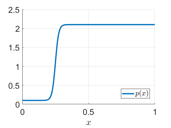
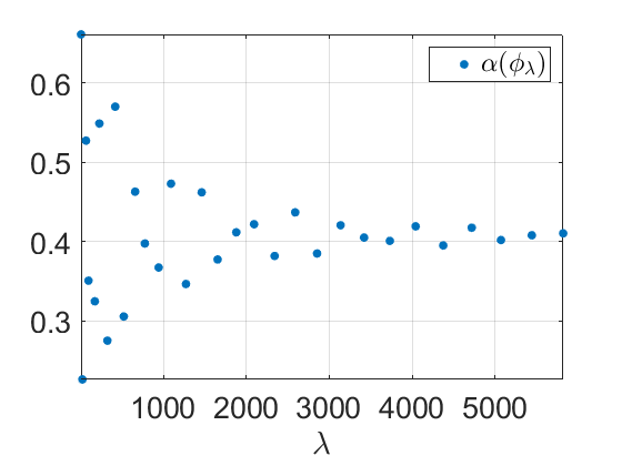
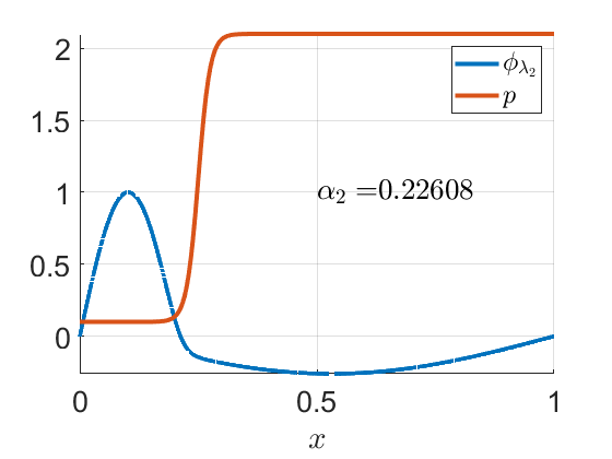
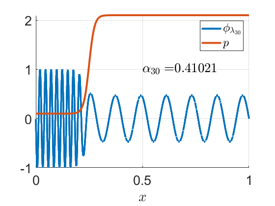
Figure 1. Localization of eigenfunctions of the Dirichlet Laplacian on $[0,1]$ with metric $p$.

Note that the most localized eigenfunctions correspond to relatively small eigenvalues, and that the localization coefficient seems to approach a constant with increasing eigenvalues. Our results, valid well beyond this single example case, predict both these empirical observations on localization.

We first derive lower and upper bounds for $\alpha(\phi_{\lambda})$ in the non-asymptotic regime, specifically showing that $\alpha(\phi_{\lambda})$ can attain relatively low values only at relatively low frequencies (small $\lambda$). Then, to complete the picture, we prove the lower and upper bounds for $\alpha(\phi_{\lambda})$ in the asymptotic regime as $\lambda\to\infty$.

The treatment of the Sturm-Liouville problem (1) when the coefficients are smooth usually starts with the Liouville transformation to the eigenvalue problem for the Schrödinger operator [1]. We work with this transformation in Section 2, but to state our second and third main results we already here define some of the involved quantities. Thus let

$$y(x)=\int_{0}^{x}\sqrt{w(s)/p(s)}ds,\quad x\in[0,L],$$

and

$$B=\int_{s=0}^{L}\sqrt{w(s)/p(s)}ds.$$

The function $y:]0,L[\to]0,B[$ is strictly increasing, and has an inverse denoted by $x(y)$. Let

$$f(y)=(w(y))p(x(y)))^{1/4},\quad y\in[0,B],$$

and

(3) $$Q(y)=f^{\prime\prime}(y)/f(y)+q(x(y))/w(x(y)),\quad y\in[0,B].$$

Write also

(4) $$a(B,\lambda)=\frac{B\|Q\|_{\infty}}{2\sqrt{\lambda}},$$

and

(5) $$b(B,\lambda)=\left(\frac{B^{3}}{12}+\frac{5B}{32\lambda}+\frac{5}{32\lambda^{3/2}}\right)^{1/4}\|Q\|_{4}/\sqrt{\lambda}.$$

Finally, for any real $\lambda$, let

$$\Phi_{\lambda}(y)=\sin(\sqrt{\lambda}y),\quad y\in[0,B].$$

Our first main result gives non-asymptotic bounds on $\alpha(\phi_{\lambda})$. Let

$$\beta(p,w)=\|w\|_{\infty}^{-2}\|p^{-1/2}w^{-3/2}\|_{\infty}^{-1}\quad{\rm and}\quad\gamma(p,w)=\|w^{-1}\|_{\infty}^{2}\|p^{1/2}w^{3/2}\|_{\infty}.$$

Theorem 1.

If

(6) $$a(B,\lambda)<1$$

and

(7) $$b(B,\lambda)<1$$

then

$$\beta(p,w)\left(\frac{1-b(B,\lambda)}{1+a(B,\lambda)}\right)^{4}\leq\frac{\alpha(\phi_{\lambda})}{\alpha(\Phi_{\lambda})}\leq\gamma(p,w)\left(\frac{1+b(B,\lambda)}{1-a(B,\lambda)}\right)^{4}.$$

Figure 2 illustrates the bounds on the localization coefficient from Theorem 1.

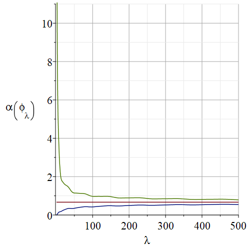
Figure 2. Lower and upper bounds on $\alpha(\phi_{\lambda})$ from Theorem 1 for the eigenvalue problem (1) after Liouville transformation, with $\beta(p,w)=1$, $\gamma(p,w)=1$, $B=1$, $\|Q\|_{\infty}=1$, and $\|Q\|_{4}=1$. The constant value is the asymptotic $2B/3$. For the chosen parameter values, the assumptions (6)–(7) are satisfied for $\lambda\gtrapprox 0.74$.

Let ${\rm BV}([0,B])$ and ${\rm AC}([0,B])$ be respectively the space of bounded variation functions, and the space of absolutely continuous functions.

Our final main result concerns the asymptotic behavior of $\alpha(\phi_{\lambda})$:

Theorem 2.

As $\lambda\rightarrow\infty$, we have

$$\beta(p,w)\frac{2B}{3}+O(\lambda^{-1/2})\leq\alpha(\phi_{\lambda})\leq\gamma(p,w)\frac{2B}{3}+O(\lambda^{-1/2})$$

when $Q\in C([0,B])$,

$$\beta(p,w)\frac{\frac{B^{2}}{4}-B(\frac{1}{4}+\|Q\|_{1}B)\lambda^{-1/2}}{\frac{3B}{8}+(\frac{9}{32}+2\|Q\|_{1}B)\lambda^{-1/2}} +O(\lambda^{-1})\leq\alpha(\phi_{\lambda})$$

$$\leq\gamma(p,w)\frac{\frac{B^{2}}{4}+B(\frac{1}{4}+\|Q\|_{1}B)\lambda^{-1/2}}{\frac{3B}{8}-(\frac{9}{32}+2\|Q\|_{1}B)\lambda^{-1/2}}+O(\lambda^{-1})$$

when $Q\in{\rm BV}([0,B])$, and

$$\beta(p,w)\frac{2B}{3}+O(\lambda^{-3/2})\leq\alpha(\phi_{\lambda})\leq\gamma(p,w)\frac{2B}{3}+O(\lambda^{-3/2})$$

when $Q\in C^{4}([0,B])\cap{\rm AC}([0,B])$ and $Q^{\prime}\in{\rm BV}([0,B])$.

Remark 1.

A straightforward calculation shows that the localization coefficient of the function $\Phi_{\lambda}$ is for any positive $\lambda$ given by

(8) $$\alpha(\Phi_{\lambda})=\frac{B^{2}/4+\cos(\sqrt{\lambda}B)^{2}/4\lambda-B\cos(\sqrt{\lambda}B)\sin(\sqrt{\lambda}B)/2\sqrt{\lambda}-\cos(\sqrt{\lambda}B)^{4}/4\lambda}{3B/8+\cos(\sqrt{\lambda}B)^{3}\sin(\sqrt{\lambda}B)/4\sqrt{\lambda}-5\cos(\sqrt{\lambda}B)\sin(\sqrt{\lambda}B)/8\sqrt{\lambda}}.$$

The eigenvalues and eigenfunctions of the Dirichlet Laplacian $-d^{2}/dy^{2}$ on $(0,B)$ are given by $\lambda_{n}=n^{2}\pi^{2}/B^{2}$ and $\Phi_{\lambda_{n}}(y)=\sin(n\pi y/B)$, respectively, with $n\in\bm{N}_{0}:=\bm{N}\setminus\{0\}=\{1,2,\dots\}$. In particular, $\alpha(\Phi_{\lambda_{n}})=2B/3$ for $n\in\bm{N}_{0}$, that is, all eigenfunctions of the Dirichlet Laplacian on $(0,B)$ have the same localization coefficient. We furthermore readily see that

(9) $$\lim_{\lambda\rightarrow\infty}\alpha(\Phi_{\lambda})=\frac{2B}{3},$$

and more precisely that, for large $\lambda$,

$$\alpha(\Phi_{\lambda}) =\frac{B^{2}/4+O(\lambda^{-1/2})}{3B/8+O(\lambda^{-1/2})}=\frac{2B}{3}\frac{1}{1+O(\lambda^{-1/2})}+O(\lambda^{-1/2})$$

(10) $$=\frac{2B}{3}+O(\lambda^{-1/2}).$$

Figure 3 shows $\alpha(\Phi_{\lambda})$ as function of $\lambda$ for the choice $B=1$.

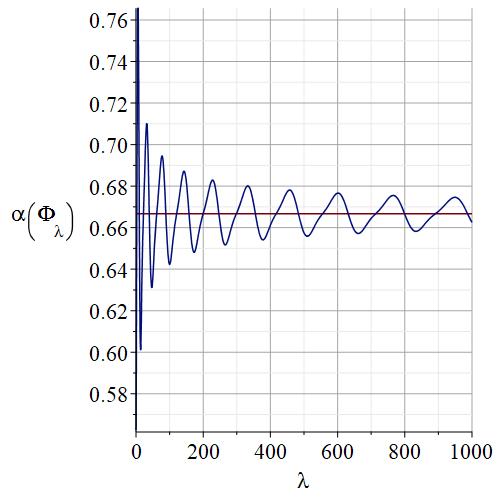
Figure 3. The localization coefficient $\alpha(\Phi_{\lambda})$ of the function $\Phi_{\lambda}(y)=\sin\sqrt{\lambda}y$, $y\in[0,B]$, for $B=1$. The constant value shown is $\alpha(\Phi_{\lambda_{n}})=2/3$, $n\in\bm{N}_{0}$, where the $\Phi_{\lambda_{n}}$ are the eigenfunctions of the Dirichlet Laplacian on the interval $[0,1]$.

Remark 2.

If $p\equiv 1$ and $w\equiv 1$ then $T$ is the Schrödinger operator $-d^{2}/dx^{2}+q(x)$. For this case, in the high-frequency limit ($\lambda\rightarrow\infty$) the localization coefficient of $\phi_{\lambda}$ approaches that of $\Phi_{\lambda}$ (so it approaches the value $2B/3$), that is, the presence of the potential $q$ becomes insignificant.

Remark 3.

It is readily seen that the lower bound on $\alpha(\phi_{\lambda})/\alpha(\Phi_{\lambda})$ in Theorem 1 is a monotonically increasing function of $\lambda$, for any fixed positive $B$. In view of this, and of the behavior of $\alpha(\Phi_{\lambda})$ discussed above, we conclude that if a solution of (1) is to exhibit high localization (relatively small value of $\alpha(\phi_{\lambda})$) then $\lambda$ must be relatively small, that is, localization is a low-frequency phenomenon.

We next focus on the localization in the eigenfunctions associated to low frequencies (small $\lambda$). In [4] the authors have given a simple but efficient way to predict the behavior of first eigenfunctions. Precisely they used the landscape function $\ell\in D(T)$, solving

(11) $$T\ell=1,\quad\ell\in D(T),$$

to identify the regions where the solution of (1) localizes. This can be observed through the following pointwise key inequality [8]

$$\phi(x)\leq\lambda\ell(x)\|\phi\|_{\infty},\quad x\in\Omega.$$

Indeed $\lambda\|\ell\|_{\infty}\geq 1$ and $\phi$ can then localize only in the region $\{x\in\Omega;\lambda\ell(x)\geq 1\}$.

Our first main result in this part of the paper thus characterizes the landscape function in terms of the first eigenfunction of the operator $T$.

Proposition 1.

Assume that $w\equiv 1$, and let $k\in\bm{N}_{0}$. If

$$T^{k}\widetilde{\ell}_{k}=1,\quad\widetilde{\ell}_{k}\in D(T^{k}),\quad\ell_{k}=\widetilde{\ell}_{k}/\|\widetilde{\ell}_{k}\|_{2},$$

as well as

$$T\phi_{1}=\lambda_{1}\phi_{1},\quad\phi_{1}\in D(T),\quad\|\phi_{1}\|_{2}=1,\quad\phi_{1}>0,\quad\lambda_{1}<\lambda_{j}\,\,\,{\rm for}\,\,\,j=2,3,\dots,$$

where $\lambda_{j},j\in\bm{N}_{0}$ is the non-decreasing sequence of eigenvalues of $T$. Then

(12) $$\|\ell_{k}-\phi_{1}\|_{\infty}\leq 2\lambda_{1}^{1/2}L\|P_{1}1\|_{2}^{-1}\left(\frac{\lambda_{1}}{\lambda_{2}}\right)^{k-1/2},$$

where $P_{1}$ is the spectral projection onto the eigenspace associated with $\lambda_{1}$.

Remark 4.

The asymptotic result in (12) shows that the convergence is exponentially fast if the fundamental gap $\lambda_{2}-\lambda_{1}$ is large enough. When $p=1$, and $q$ is a weakly convex potential it is known that [7]

$$\lambda_{2}-\lambda_{1}\geq\frac{3\pi^{2}}{L^{2}}.$$

The inequality conjectured by Yau [9] is still an open problem in higher dimensions. It turns out that this spectral gap also determines the rate at which positive solutions of the heat equation tend to their projections onto the first eigenspace.

Proposition 2.

Assume that $w\equiv 1$, and let $\lambda_{j}$, $j\in\bm{N}_{0}$, be the non-decreasing sequence of eigenvalues of $T$. Let $P_{j}$ be the spectral projection onto the eigenspace associated with $\lambda_{j}$. Let $k$, $n_{0}\in\bm{N}_{0}$, and $t\in]\lambda_{n_{0}+1}^{-1},\lambda_{n_{0}}^{-1}[$. If

$$(tT)^{k}\ell_{k,t}=1,\quad\ell_{k,t}\in D(T^{k}),$$

then

(13) $$\|\ell_{k,t}-\sum_{j=1}^{n_{0}}\frac{1}{(t\lambda_{j})^{k}}P_{j}1\|_{\infty}\leq\frac{L}{t^{1/2}}\frac{1}{(t\lambda_{n_{0}+1})^{k-1/2}}.$$

Remark 5.

The value of $t$ fix the number of the eigenfunctions covered by the generalized landscape function $\ell_{t,k}$. Notice that $t\in]\lambda_{n_{0}+1}^{-1},\lambda_{n_{0}}^{-1}[$ is equivalent to

$$\frac{1}{t\lambda_{n_{0}+1}}<1<\frac{1}{t\lambda_{n_{0}}},$$

which implies that the contribution of the eigenfunctions $P_{j}1,\;j>n_{0}$ in the localization of $\ell_{k,t}$ is exponentially small for large $k$ while the contribution of $P_{j}1$ for $1\leq j\leq n_{0}$ can be exponentially large if in addition $P_{j}1$ is not zero. These observations are confirmed in Section 6 by several numerical tests. Finally the results of Propositions 1 and 2 are still valid for $w$ non-constant and sufficiently smooth ($\|\cdot\|_{2}$ should be substituted by $\|\cdot\|_{L^{2}(]0,L[;wdx)})$).

Theorem 1 is proved in Section 2 using a Volterra integral equation representation of solutions of (1) given by Fulton [5], while Theorem 2 is proved in Section 3 via the asymptotic expansions of $\phi_{\lambda}$, as $\lambda\rightarrow\infty$, given in Fulton and Pruess [6]. Finally, we prove Propositions 1 and 2 in respectively Sections 4 and 5 using the power method.

2. Proof of Theorem 1 (non-asymptotic bounds on $\alpha(\phi_{\lambda})$)

Using the Liouville transformation

$$y(x)=\int_{0}^{x}\sqrt{w(s)/p(s)}ds\,\,\,\text{for}\,\,x\in[0,L];\quad B=y(L);$$

$$f(y)=(w(x(y))p(x(y)))^{1/4},\quad y\in[0,B];$$

(14) $$v_{\lambda}(y)=\phi_{\lambda}(x(y))f(y),\quad y\in[0,B];$$

and

$$\quad Q(y)=f^{\prime\prime}(y)/f(y)+q(x(y))/w(x(y)),\quad y\in[0,B],$$

we recast the problem (1) in the Liouville normal form [6, pp. 303–304]

(15) $$\left\{\begin{array}[]{rcl}-v_{\lambda}^{\prime\prime}+Q(y)v_{\lambda}&=&\lambda v_{\lambda},\quad y\in(0,B),\\ v_{\lambda}(0)=v_{\lambda}(B)&=&0.\end{array}\right.$$

It follows from our assumptions on $p$, $w$ and $q$ that $Q\in C([0,B])$, hence $Q\in L^{t}([0,B])$ for $t\in[1,\infty]$. Now

$$\int_{x=0}^{L}\phi_{\lambda}(x)^{2}dx=\int_{y=0}^{B}\frac{v_{\lambda}(y)^{2}}{w(x(y))}dy\in\left[\|w\|^{-1}_{\infty},\|w^{-1}\|_{\infty}\right]\times\int_{y=0}^{B}v_{\lambda}(y)^{2}dy$$

and

$$\int_{x=0}^{L}\phi_{\lambda}(x)^{4}dx =\int_{y=0}^{B}\frac{v_{\lambda}(y)^{4}}{p(x(y))^{1/2}w(x(y))^{3/2}}dy$$

$$\in\left[\|p^{1/2}w^{3/2}\|^{-1}_{\infty},\|p^{-1/2}w^{-3/2}\|_{\infty}\right]\times\int_{y=0}^{B}v_{\lambda}(y)^{4}dy,$$

so it remains to examine $\|v_{\lambda}\|_{2}^{2}$ and $\|v_{\lambda}\|_{4}^{4}$. To this end we recall from Fulton and Pruess [6, p. 308] that a solution of the ODE in (15), normalized such that $v_{\lambda}(0)=0$ and $v^{\prime}_{\lambda}(0)=(w(0)p(0))^{-1/4}\neq 0$, satisfies the associated Volterra integral equation

(16) $$\left({\rm Id}-\frac{1}{\sqrt{\lambda}}K_{Q}\right)v_{\lambda}(y)=\frac{v^{\prime}_{\lambda}(0)}{\sqrt{\lambda}}\Phi_{\lambda}(y),\quad y\in[0,B],$$

where for any $u\in C^{2}([0,B])$ we have

$$K_{Q}u(y)=\int_{z=0}^{y}Q(z)\sin(\sqrt{\lambda}(y-z))u(z)dz,\quad y\in]0,B[.$$

Now write $\|K_{Q}\|_{t}$ for the operator norm of $K_{Q}$ as a mapping from $L^{t}(]0,B[)$ to $L^{t}(]0,B[)$.

Lemma 1.

For every positive $\lambda$ we have

$$\|K_{Q}\|^{2}_{2}\leq\frac{B^{2}}{4}\|Q\|^{2}_{\infty}$$

and

$$\|K_{Q}\|^{4}_{4}\leq\left(\frac{B^{3}}{12}+\frac{5B}{32\lambda}+\frac{5}{32\lambda^{3/2}}\right)\|Q\|^{4}_{4}.$$

Proof.

The estimates follow readily from applying Hölder’s inequality. We have

$$\|K_{Q}u\|^{2}_{2} \leq\|Q\|_{\infty}^{2}\|u\|_{2}^{2}\int_{y=0}^{B}\|\sin(\sqrt{\lambda}(y-\cdot))\|_{L^{2}(]0,y[)}^{2}dy$$

$$=\|Q\|_{\infty}^{2}\|u\|_{2}^{2}\int_{y=0}^{B}\left(\frac{y}{2}-\frac{\cos\sqrt{\lambda}y\sin\sqrt{\lambda}y}{2\sqrt{\lambda}}\right)$$

$$=\frac{\|Q\|_{\infty}^{2}}{4}\|u\|_{2}^{2}\left(B^{2}-\frac{\sin^{2}\sqrt{\lambda}B}{\lambda}\right)$$

$$\leq\frac{\|Q\|_{\infty}^{2}B^{2}}{4}\|u\|_{2}^{2},\quad u\in L^{2}(]0,B[),$$

as well as

$$\|K_{Q}u\|^{4}_{4} \leq\|Q\|_{4}^{4}\|u\|_{4}^{4}\int_{y=0}^{B}\|\sin(\sqrt{\lambda}(y-\cdot))\|_{L^{2}(]0,y[)}^{4}dy$$

$$=\|Q\|_{4}^{4}\|u\|_{4}^{4}\left(\frac{B^{3}}{12}+\frac{B\cos(\sqrt{\lambda}B)^{2}}{4\lambda}-\frac{\sin\sqrt{\lambda}B\cos(\sqrt{\lambda}B)^{3}}{16\lambda^{3/2}}\right.$$

$$\left.-\frac{3B}{32\lambda}-\frac{3\cos\sqrt{\lambda}B\sin\sqrt{\lambda}B}{32\lambda^{3/2}}\right)$$

$$\leq\|Q\|_{4}^{4}\left(\frac{B^{3}}{12}+\frac{5B}{32\lambda}+\frac{5}{32\lambda^{3/2}}\right)\|u\|_{4}^{4},\quad u\in L^{4}([0,B]),$$

∎

We have from (16) and from Lemma 1 that, for all positive $\lambda$,

$$\|v_{\lambda}\|_{2} \geq\lambda^{-1/2}|v^{\prime}_{\lambda}(0)|\|\Phi_{\lambda}\|_{2}-\lambda^{-1/2}\|K_{Q}\|_{2}\|v_{\lambda}\|_{2}$$

$$\geq\lambda^{-1/2}|v^{\prime}_{\lambda}(0)|\|\Phi_{\lambda}\|_{2}-\lambda^{-1/2}B\|Q\|_{\infty}\|v_{\lambda}\|_{2}/2,$$

$$\|v_{\lambda}\|_{2} \leq\lambda^{-1/2}|v^{\prime}_{\lambda}(0)|\|\Phi_{\lambda}\|_{2}+\lambda^{-1/2}\|K_{Q}\|_{2}\|v_{\lambda}\|_{2}$$

$$\leq\lambda^{-1/2}|v^{\prime}_{\lambda}(0)|\|\Phi_{\lambda}\|_{2}+\lambda^{-1/2}B\|Q\|_{\infty}\|v_{\lambda}\|_{2}/2,$$

$$\|v_{\lambda}\|_{4} \geq\lambda^{-1/2}|v^{\prime}_{\lambda}(0)|\|\Phi_{\lambda}\|_{4}-\lambda^{-1/2}\|K_{Q}\|_{4}\|v_{\lambda}\|_{4}$$

$$\geq\lambda^{-1/2}|v^{\prime}_{\lambda}(0)|\|\Phi_{\lambda}\|_{4}-\lambda^{-1/2}\left(\frac{B^{3}}{12}+\frac{5B}{32\lambda}+\frac{5}{32\lambda^{3/2}}\right)^{1/4}\|Q\|_{4}\|v_{\lambda}\|_{4},$$

and

$$\|v_{\lambda}\|_{4} \leq\lambda^{-1/2}|v^{\prime}_{\lambda}(0)|\|\Phi_{\lambda}\|_{4}+\lambda^{-1/2}\|K_{Q}\|_{4}\|v_{\lambda}\|_{4}$$

$$\leq\lambda^{-1/2}|v^{\prime}_{\lambda}(0)|\|\Phi_{\lambda}\|_{4}+\lambda^{-1/2}\left(\frac{B^{3}}{12}+\frac{5B}{32\lambda}+\frac{5}{32\lambda^{3/2}}\right)^{1/4}\|Q\|_{4}\|v_{\lambda}\|_{4}.$$

Specifically, for $B\|Q\|_{\infty}/2<\sqrt{\lambda}$ (assumption (6)) and

$$\left(\frac{B^{3}}{12}+\frac{5B}{32\lambda}+\frac{5}{32\lambda^{3/2}}\right)^{1/4}\|Q\|_{4}<\sqrt{\lambda}$$

(assumption (7)), we have

$$\left(\frac{1-b(B,\lambda)}{1+a(B,\lambda)}\right)^{4}\leq\frac{\alpha(v_{\lambda})}{\alpha(\Phi_{\lambda})}\leq\left(\frac{1+b(B,\lambda)}{1-a(B,\lambda)}\right)^{4}.$$

3. Proof of Theorem 2 (asymptotic bounds on $\alpha(\phi_{\lambda})$)

The first part of Theorem 2 follows from the fact that

$$\frac{1\mp b(B,\lambda)}{1\pm a(B,\lambda)}=1+O(\lambda^{-1/2}),\quad\lambda\rightarrow\infty,$$

together with (1) and the estimates in Theorem 1.

Next, if $Q\in{\rm BV}([0,B])$ then we can use the asymptotic expansion of $v_{\lambda}$ from (15) given by Eq. (3.3)_2N of Fulton and Pruess [6] with $N=1$, and get

$$v_{\lambda}(y)/v_{\lambda}^{\prime}(0)=\lambda^{-1/2}\sin(\lambda^{1/2}y)-\frac{1}{2\lambda}\int_{0}^{y}Q(s)ds\cdot\cos(\lambda^{1/2}y)+O(\lambda^{-3/2}),\quad y\in[0,B],$$

where the remainder $O(\lambda^{-3/2})$ is uniform in $y\in[0,B]$. This, in turn, implies

$$\frac{\|v_{\lambda}\|_{2}^{4}}{v_{\lambda}^{\prime}(0)^{4}} =\lambda^{-2}\frac{B^{2}}{4}$$

$$-\lambda^{-5/2}B\left(\frac{1}{4}\sin(2B\lambda^{1/2})+\int_{y=0}^{B}\int_{s=0}^{y}Q(s)ds\sin(\lambda^{1/2}y)\cos(\lambda^{1/2}y)dy\right)+O(\lambda^{-3})$$

and

$$\frac{\|v_{\lambda}\|_{4}^{4}}{v_{\lambda}^{\prime}(0)^{4}} =\lambda^{-2}\frac{3B}{8}$$

$$+\lambda^{-5/2}\Biggl{(}\frac{\sin(4B\lambda^{1/2})-8\sin(2B\lambda^{1/2})}{32}\Biggr{.}$$

$$\Biggl{.}\qquad-2\int_{y=0}^{B}\int_{s=0}^{y}Q(s)ds\sin^{3}(\lambda^{1/2}y)\cos(\lambda^{1/2}y)dy\Biggr{)}+O(\lambda^{-3})$$

as $\lambda\rightarrow\infty$. Thus $c_{-}\leq\lambda^{2}\|v_{\lambda}\|_{2}^{4}/v_{\lambda}^{\prime}(0)^{4}\leq c_{+}$ with

$$c_{\pm}=\frac{B^{2}}{4}\pm\lambda^{-1/2}B\left(\frac{1}{4}+B\|Q\|_{1}\right)+O(\lambda^{-1}),\quad\lambda\rightarrow\infty,$$

and $d_{-}\leq\lambda^{2}\|v_{\lambda}\|_{4}^{4}/v_{\lambda}^{\prime}(0)^{4}\leq d_{+}$ with

$$d_{\pm}=\frac{3B}{8}\pm\lambda^{-1/2}\left(\frac{9}{32}+2B\|Q\|_{1}\right)+O(\lambda^{-1}),\quad\lambda\rightarrow\infty.$$

Finally, if $Q\in{\rm AC}([0,B])$ and $Q^{\prime}\in{\rm BV}([0,B])$ then we can use the asymptotic expansion of $v_{\lambda}$ given by [6, Eq. (3.3)_2N+1] with $N=1$, to get

$$v_{\lambda}(y)/v^{\prime}_{\lambda}(0) =\lambda^{-1/2}\sin(\lambda^{1/2}y)-\lambda^{-1}\frac{1}{2}\cos(\lambda^{1/2}y)\int_{0}^{y}Q(s)ds$$

(17) $$+\lambda^{-3/2}\frac{1}{4}\sin(\lambda^{1/2}y)\left(\int_{0}^{y}Q(s)\int_{0}^{s}Q(\tau)d\tau ds+Q(0)+Q(y)\right)+O(\lambda^{-2}),$$

where the remainder $O(\lambda^{-2})$ is uniform in $y$. This, in turn, implies

$$\frac{\|v_{\lambda}\|_{2}^{4}}{v^{\prime}_{\lambda}(0)^{4}} =\lambda^{-2}\frac{B^{2}}{4}$$

$$-\lambda^{-5/2}B\left(\frac{\sin(2B\lambda^{1/2})}{4}+\int_{0}^{B}\sin(\lambda^{1/2}y)\cos(\lambda^{1/2}y)\int_{0}^{y}Q(s)dsdy\right)$$

$$+\lambda^{-3}B\Biggl{(}\frac{1}{4}\int_{0}^{B}\cos^{2}(\lambda^{1/2}y)\left(\int_{0}^{y}Q(s)ds\right)^{2}dy\Biggr{.}$$

$$\Biggl{.}+\frac{1}{2}\int_{0}^{B}\sin^{2}(\lambda^{1/2}y)\left(\int_{0}^{y}Q(s)\int_{0}^{s}Q(\tau)d\tau ds+Q(0)+Q(y)\right)dy\Biggr{)}+O(\lambda^{-7/2})$$

and

$$\frac{\|v_{\lambda}\|_{4}^{4}}{v^{\prime}_{\lambda}(0)^{4}} =\lambda^{-2}\frac{3B}{8}$$

$$+\lambda^{-5/2}\left(\frac{\sin(4B\lambda^{1/2})-8\sin(2B\lambda^{1/2})}{32}-2\int_{y=0}^{B}\sin^{3}(\lambda^{1/2}y)\cos(\lambda^{1/2}y)\int_{0}^{y}Q(s)dsdy\right)$$

$$+\lambda^{-3}\Biggl{(}\frac{3}{2}\int_{0}^{B}\sin^{2}(\lambda^{1/2}y)\cos^{2}(\lambda^{1/2}y))\left(\int_{0}^{y}Q(s)ds\right)^{2}dy\Biggr{.}$$

$$\Biggl{.}+\int_{0}^{B}\sin^{4}(\lambda^{1/2}y)\left(\int_{0}^{y}Q(s)\int_{0}^{s}Q(\tau)d\tau ds+Q(0)+Q(y)\right)dy\Biggr{)}+O(\lambda^{-7/2}).$$

Now each eigenvalue $\lambda$ is a zero of $\lambda\mapsto v_{\lambda}(B)$ [6, p. 319, Case 4], and in light of (3) we therefore have

$$\sin(\lambda^{1/2}B)=\lambda^{-1/2}\frac{1}{2}\int_{0}^{B}Q(s)ds\cdot\cos(\lambda^{1/2}B)+O(\lambda^{-3/2}),$$

$$\sin^{2}(\lambda^{1/2}B)=\lambda^{-1}\frac{1}{4}\left(\int_{0}^{B}Q(s)ds\right)^{2}\cos^{2}(\lambda^{1/2}B)+O(\lambda^{-2}),\quad\cos^{2}(\lambda^{1/2}B)=1+O(\lambda^{-1}),$$

$$\sin(2\lambda^{1/2}B)=\lambda^{-1/2}\int_{0}^{B}Q(s)ds\cdot\cos^{2}(\lambda^{1/2}B)+O(\lambda^{-3/2}),$$

and

$$\sin(4\lambda^{1/2}B)=\lambda^{-1/2}2\int_{0}^{B}Q(s)ds\cdot\cos(2\lambda^{1/2}B)\cos^{2}(\lambda^{1/2}B)+O(\lambda^{-3/2}).$$

Also, using integration by parts, we find for any $\phi,\psi\in C^{4}([0,B])$ with $\phi(0)=0$ that

$$\int_{0}^{B}\sin(\lambda^{1/2}y)\cos(\lambda^{1/2}y)\phi(y)dy =\lambda^{-1/2}\left(\frac{\sin^{2}(\lambda^{1/2}B)}{2}-\frac{1}{4}\right)\phi(B)+O(\lambda^{-1})$$

$$=-\lambda^{-1/2}\frac{1}{4}\phi(B)+O(\lambda^{-1}),$$

$$\int_{0}^{B}\cos^{2}(\lambda^{1/2}y)\phi(y)dy =\frac{1}{2}\int_{0}^{B}\phi(y)dy+\lambda^{-1/2}\frac{\sin(2\lambda^{1/2}B)}{4}\phi(B)+O(\lambda^{-1})$$

$$=\frac{1}{2}\int_{0}^{B}\phi(y)dy+O(\lambda^{-1}),$$

$$\int_{0}^{B}\sin^{2}(\lambda^{1/2}y)\psi(y)dy =\frac{1}{2}\int_{0}^{B}\psi(y)dy-\lambda^{-1/2}\frac{\sin(2\lambda^{1/2}B)}{4}\psi(B)+O(\lambda^{-1})$$

$$=\frac{1}{2}\int_{0}^{B}\psi(y)dy+O(\lambda^{-1}),$$

$$\int_{0}^{B}\sin^{3}(\lambda^{1/2}y)\cos(\lambda^{1/2}y)\phi(y)dy =\lambda^{-1/2}\left(\frac{\sin^{4}(\lambda^{1/2}B)}{4}-\frac{3}{32}\right)\phi(B)+O(\lambda^{-1})$$

$$=-\lambda^{-1/2}\frac{3}{32}\phi(B)+O(\lambda^{-1}),$$

$$\int_{0}^{B}\sin^{2}(\lambda^{1/2}y)\cos^{2}(\lambda^{1/2}y)\phi(y)dy =\frac{1}{8}\int_{0}^{B}\phi(y)dy$$

$$+\lambda^{-1/2}\Biggl{(}\frac{\sin(2\lambda^{1/2}B)-4\sin(\lambda^{1/2}B)\cos^{3}(\lambda^{1/2}B)}{16}\phi(B)\Biggr{.}$$

$$\Biggl{.}-\frac{\cos^{4}(\lambda^{1/2}B)}{2}\phi^{\prime}(B)+\frac{3}{16}\phi^{\prime}(B)+\frac{5}{16}\phi^{\prime}(0)\Biggr{)}+O(\lambda^{-1})$$

$$=\frac{1}{8}\int_{0}^{B}\phi(y)dy+\lambda^{-1/2}\frac{5}{16}\left(\phi^{\prime}(0)-\phi^{\prime}(B)\right)+O(\lambda^{-1}),$$

and

$$\int_{0}^{B}\sin^{4}(\lambda^{1/2}y)\psi(y)dy =\frac{3}{8}\int_{0}^{B}\psi(y)dy$$

$$-\lambda^{-1/2}\left(\frac{\sin^{3}(\lambda^{1/2}B)\cos(\lambda^{1/2}B)}{4}+\frac{3\sin(2\lambda^{1/2}B)}{16}\right)\psi(B)+O(\lambda^{-1})$$

$$=\frac{3}{8}\int_{0}^{B}\psi(y)dy+O(\lambda^{-1}).$$

Using these expansions, we get

$$\lambda^{2}\frac{\|v_{\lambda}\|_{2}^{4}}{v^{\prime}_{\lambda}(0)^{4}} =\frac{B^{2}}{4}+\lambda^{-1}\frac{B}{4}\Biggl{[}\frac{1}{2}\int_{0}^{B}\left(\int_{0}^{y}Q(s)ds\right)^{2}dy\Biggr{.}$$

$$\Biggl{.}+\int_{0}^{B}\left(\int_{0}^{y}Q(s)\int_{0}^{s}Q(\tau)d\tau ds+Q(0)+Q(y)\right)dy\Biggr{]}+O(\lambda^{-3/2})$$

and

$$\lambda^{2}\frac{\|v_{\lambda}\|_{4}^{4}}{v^{\prime}_{\lambda}(0)^{4}} =\frac{3B}{8}$$

$$+\lambda^{-1}\frac{3}{8}\Biggl{[}\frac{1}{2}\int_{0}^{B}\left(\int_{0}^{y}Q(s)ds\right)^{2}dy\Biggr{.}$$

$$\Biggl{.}+\int_{0}^{B}\left(\int_{0}^{y}Q(s)\int_{0}^{s}Q(\tau)d\tau ds+Q(0)+Q(y)\right)dy\Biggr{]}+O(\lambda^{-3/2}).$$

Note that the factors multiplying $\lambda^{0}$ and $\lambda^{-1}$ in $\|v_{\lambda}\|_{2}^{4}$ are proportional to those in $\|v_{\lambda}\|_{4}^{4}$, with the proportionality constant $2B/3$. We thus have

$$\alpha(v_{\lambda})=\frac{B^{2}/4+\lambda^{-1}s+O(\lambda^{-3/2})}{(3/2B)(B^{2}/4+\lambda^{-1}s+O(\lambda^{-3/2}))}=\frac{2B}{3}+O(\lambda^{-3/2}),$$

where

$$s=\frac{B}{4}\Biggl{[}\frac{1}{2}\int_{0}^{B}\left(\int_{0}^{y}Q(s)ds\right)^{2}dy+\int_{0}^{B}\left(\int_{0}^{y}Q(s)\int_{0}^{s}Q(\tau)d\tau ds+Q(0)+Q(y)\right)dy\Biggr{]}.$$

4. Proof of Proposition 1

By construction $T$ is self-adjoint and diagonalizable. Hence it can be written in the following form

(18) $$T=\sum_{j=1}^{\infty}\lambda_{j}P_{j},$$

where $(\lambda_{j})_{j\in\bm{N}_{0}}$ is the strictly increasing sequence of eigenvalues of $T$, and $P_{j}$ are the orthogonal projections onto the eigenspaces associated to $\lambda_{j},\;j\in\bm{N}_{0}.$

Since $\ell_{k}\in D(T)$, it has the following expansion

$$\ell_{k}=\tilde{\ell}_{k}/\|\tilde{\ell}_{k}\|_{2},\quad\tilde{\ell}_{k}=\sum_{j=1}^{\infty}\lambda_{j}^{-k}P_{j}1.$$

Straightforward computations give

(19) $$\|\lambda_{1}^{k}\tilde{\ell}_{k}-P_{1}1\|_{2}\leq L^{1/2}\left(\frac{\lambda_{1}}{\lambda_{2}}\right)^{k},\quad\textrm{and }\|P_{1}1\|_{2}\leq\|\lambda_{1}^{k}\tilde{\ell}_{k}\|_{2}.$$

We then deduce

(20) $$\|\lambda_{1}^{k}\tilde{\ell}_{k}\|_{2}-\|P_{1}1\|_{2}\leq L^{1/2}\left(\frac{\lambda_{1}}{\lambda_{2}}\right)^{k}.$$

Similarly, since $T\tilde{\ell}_{k}\in L^{2}(]0,L[)$, we have

(21) $$\|\lambda_{1}^{k}T^{1/2}\tilde{\ell}_{k}-T^{1/2}P_{1}1\|_{2}\leq(\lambda_{1}L)^{1/2}\left(\frac{\lambda_{1}}{\lambda_{2}}\right)^{k-1/2}.$$

Recall that $\phi_{1}>0$, which implies $\|P_{1}1\|_{2}>0$ and $\phi_{1}=P_{1}1/\|P_{1}1\|_{2}$. Now combining inequalities (19), (20) and (21), we get

$$\|T^{1/2}\ell_{k}-T^{1/2}\phi_{1}\|_{2}\leq\|\lambda_{1}^{k}T^{1/2}\tilde{\ell}_{k}-T^{1/2}P_{1}1\|_{2}\|P_{1}1\|_{2}^{-1}+\lambda_{1}^{1/2}\left(\|\lambda_{1}^{k}\tilde{\ell}_{k}\|_{2}-\|P_{1}1\|_{2}\right)\|P_{1}1\|_{2}^{-1}$$

(22) $$\leq 2(\lambda_{1}L)^{1/2}\left(\frac{\lambda_{1}}{\lambda_{2}}\right)^{k-1/2}\|P_{1}1\|_{2}^{-1}.$$

On the other hand, we have

$$|\varphi(x)|\leq\int_{0}^{x}|\varphi^{\prime}(s)|ds\leq L^{1/2}\|\varphi^{\prime}\|_{2},\quad\forall x\in]0,L[,$$

for all $\varphi\in C^{\infty}_{0}(]0,L[)$.

Since $C^{\infty}_{0}(]0,L[)$ is dense in $D(T^{1/2})$, we get

(23) $$\|\varphi\|_{\infty}\leq L^{1/2}\|T^{1/2}\varphi\|_{2},\quad\forall\varphi\in D(T^{1/2}).$$

Combining inequalities (23) and (22), we obtain the desired result.

5. Proof of Proposition 2

Using the spectral expansion (18), we get

$$\ell_{k,t}=\sum_{j=1}^{\infty}\frac{1}{(t\lambda_{j})^{k}}P_{j}1.$$

Hence

$$T^{1/2}\left(\ell_{k,t}-\sum_{j=1}^{n_{0}}\frac{1}{(t\lambda_{j})^{k}}P_{j}1\right)=\sum_{j=n_{0}+1}^{\infty}\frac{1}{(t\lambda_{j})^{k}}T^{1/2}P_{j}1.$$

Therefore

(24) $$\left\|T^{1/2}\left(\ell_{k,t}-\sum_{j=1}^{n_{0}}\frac{1}{(t\lambda_{j})^{k}}P_{j}1\right)\right\|_{2}\leq\frac{L^{1/2}}{t^{1/2}}\frac{1}{(t\lambda_{n_{0}+1})^{k-1/2}}.$$

Applying again the Sobolev inequality (23), we recover the final estimate.

6. The landscape function: numerical tests

We start by illustrating the consequences of Proposition 1. For Figure 4 we use $L=1$ and

$$p(x)=\tanh(40x/L-10)+1.1,\quad q(x)=0,\quad x\in[0,L],$$

as in (2) in Section 1), while Figure 5 shows the graphs of

$$p(x)=\tanh(40x/L-20)+1.1,\quad q(x)=2+\sin(2\pi x),\quad x\in[0,L],$$

used, with $L=1$, for the results of Figure 6. Finally, Figure 7 shows the functions

$$p(x)=\tanh(40x/L-10)+1.1,\quad q(x)=2+\sin(2\pi x),\quad x\in[0,L],$$

used, with $L=5$, for the results of Figure 8.

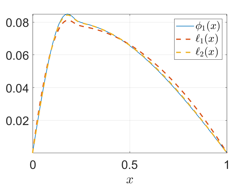
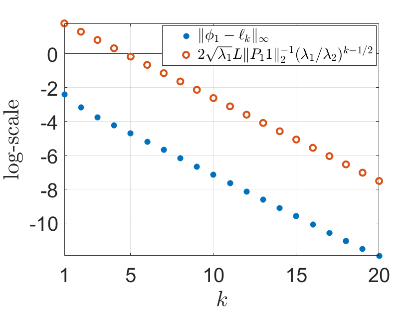
Figure 4. Left: the functions $\ell_{k}$ approach the first eigenvector $\phi_{1}$ pointwise as $k$ increases. Right: actual value vs. upper bound on $\|\phi_{1}-\ell_{k}\|_{\infty}$, see Proposition 1.

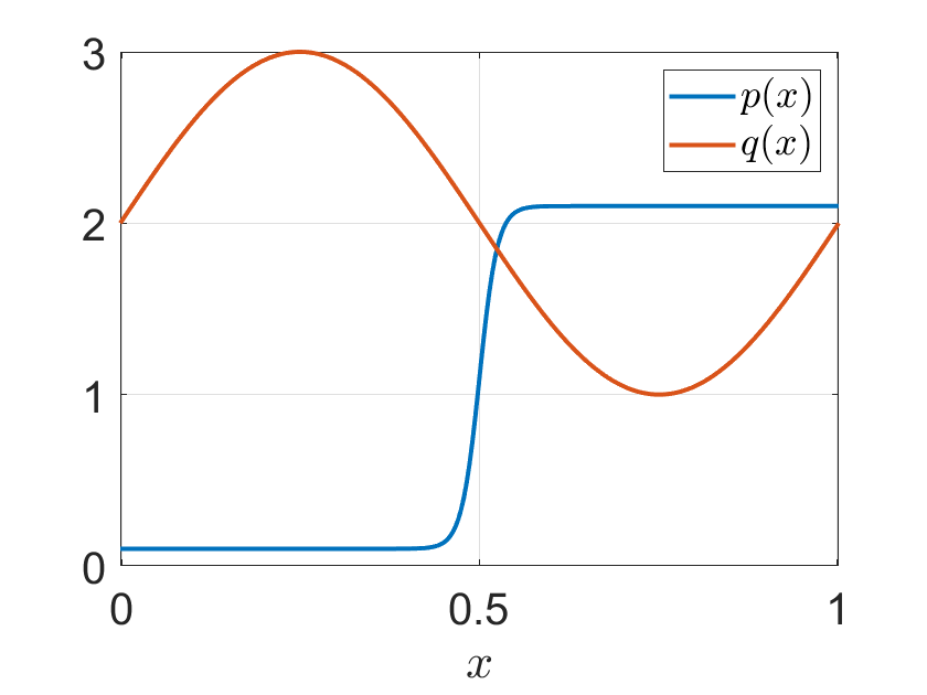
Figure 5. The functions $p(x)$ and $q(x)$ used for the results of Figure 6.

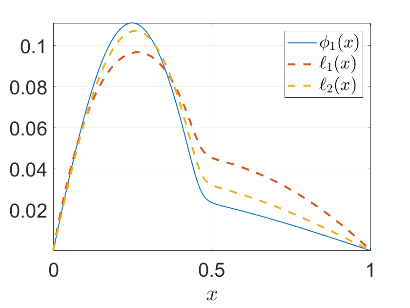
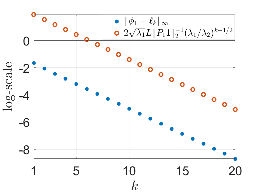
Figure 6. Left: the functions $\ell_{k}$ approach the first eigenvector $\phi_{1}$ pointwise as $k$ increases. Right: actual value vs. upper bound on $\|\phi_{1}-\ell_{k}\|_{\infty}$, see Proposition 1.

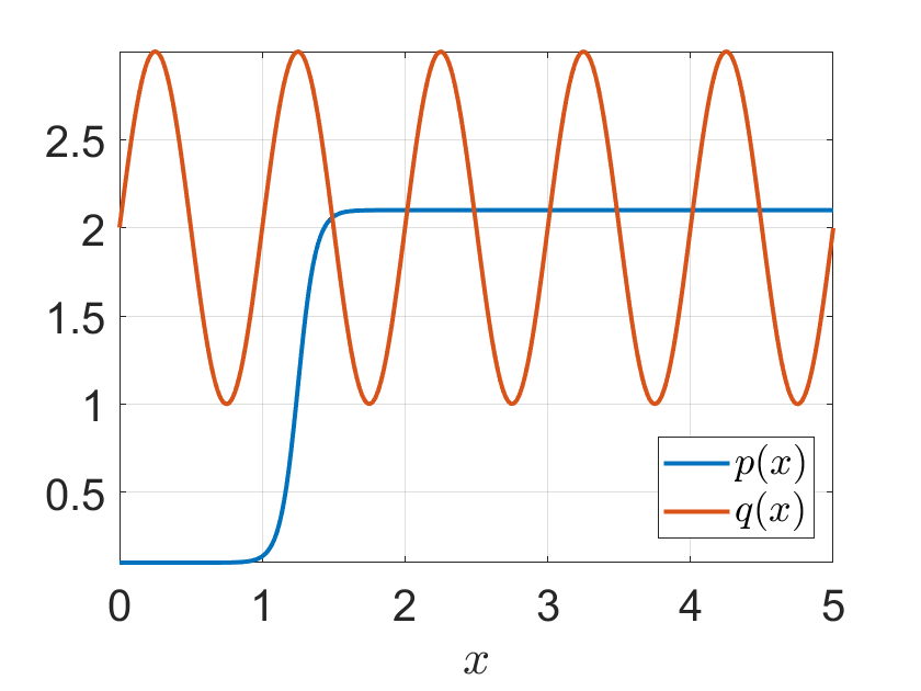
Figure 7. The functions $p(x)$ and $q(x)$ used for the results of Figure 8.

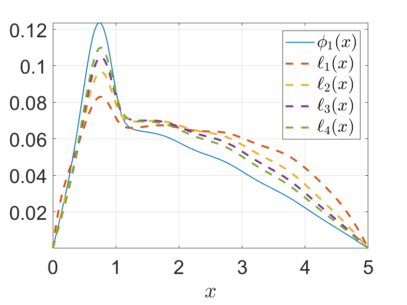
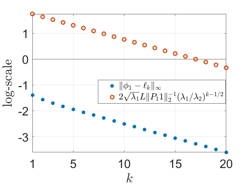
Figure 8. Left: the functions $\ell_{k}$ approach the first eigenvector $\phi_{1}$ pointwise as $k$ increases. Right: actual value vs. upper bound on $\|\phi_{1}-\ell_{k}\|_{\infty}$, see Proposition 1.

Next, in Figure 9 we illustrate the validity of the upper bound on $\|\ell_{k,t}-\sum_{j=1}^{n_{0}}(t\lambda_{j})^{-k}P_{j}1\|_{\infty}$, as given in Proposition 2. Since the constants $(t\lambda_{j})^{-1}$, $j=1,\dots,n_{0}$, are greater than 1, the numerical error present in the above $L^{\infty}$-norm can grow exponentially with $k$. To avoid this numerical instability, in Figure 9 we plot the equivalent quantity $\|\sum_{j=n_{0}+1}^{\infty}(t\lambda_{j})^{-k}(t\lambda_{j})^{-k}P_{j}1\|_{\infty}$, with the series truncated at $j=20$.

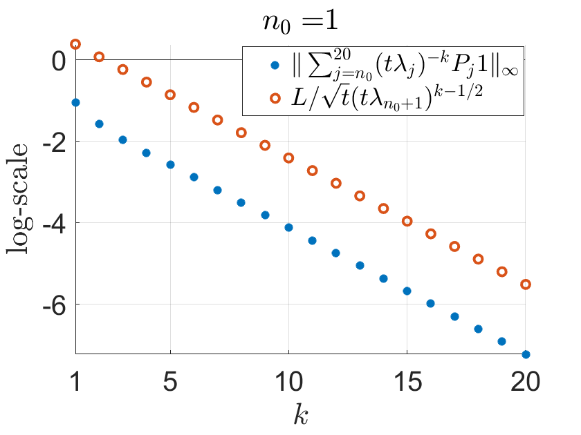
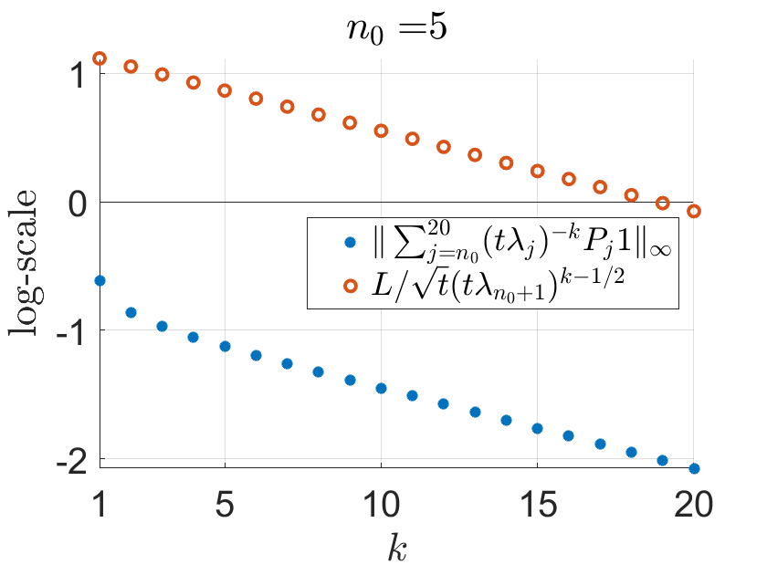
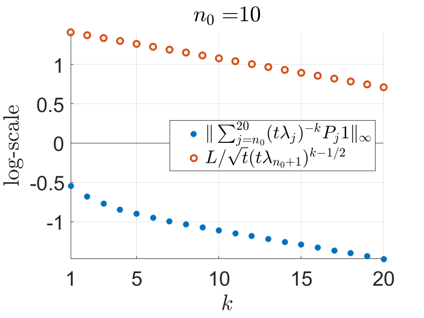
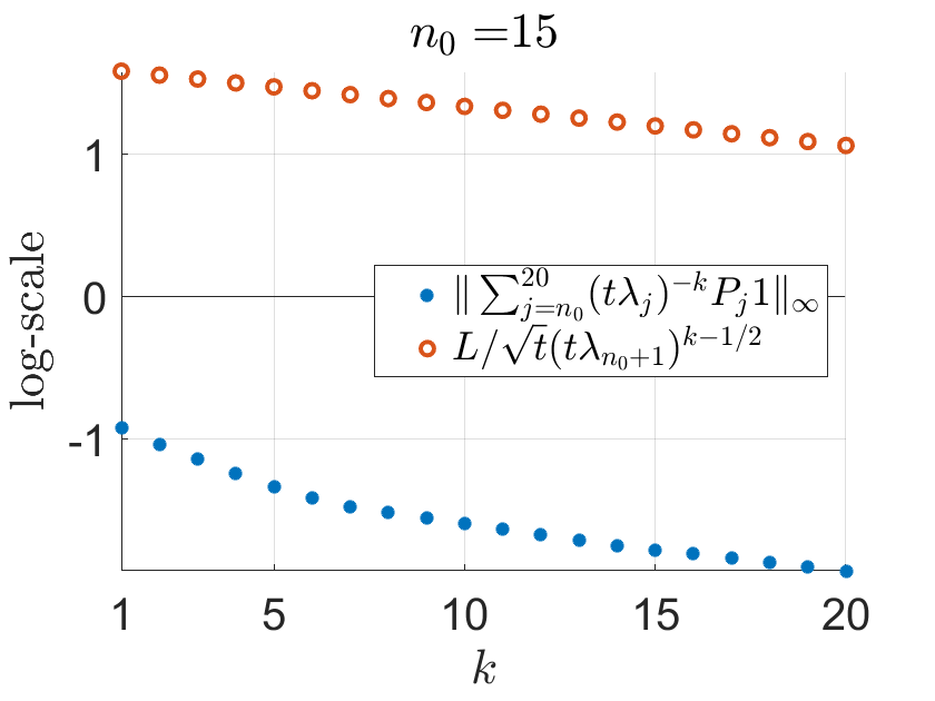
Figure 9. Illustration of the upper bound of Proposition 2 for different values of $n_{0}$.

References

- [1] G. Bao and F. Triki, Stability for the multifrequency inverse medium problem, Journal of Differential Equations 269 (2020), no. 9, 7106–7128.
- [2] S. Félix, M. Asch, M. Filoche, and B. Sapoval, Localization and increased damping in irregular acoustic cavities, Journal of Sound and Vibration 299 (2007), 965–976.
- [3] M. Filoche, S. Mayaboroda, and B. Patterson, Localization of eigenfunctions of a one-dimensional elliptic operator, Contemporary Mathematics 581 (2012), 99–116.
- [4] M. Filoche and S. Mayboroda, Universal mechanism for Anderson and weak localization, Proceedings of the National Academy of Sciences 109 (2012), no. 37, 14761–14766.
- [5] C. T. Fulton, An Integral Equation Iterative Scheme for Asymptotic Expansions of Spectral Quantities of Regular Sturm-Liouville Problems, Journal of Integral Equations 4 (1982), 163–172.
- [6] C. T. Fulton and S. A. Pruess, Eigenvalue and Eigenfunction Asymptotics for Regular Sturm-Liouville Problems, Journal of Mathematical Analysis and Applications 188 (1994), 297–340.
- [7] R. Lavine, The eigenvalue gap for one-dimensional convex potentials, Proceedings of the American mathematical Society 121 (1994), no. 3, 815–821.
- [8] C. B. Moler and L. E. Payne, Bounds for eigenvalues and eigenvectors of symmetric operators, SIAM Journal on Numerical Analysis 5 (1968), no. 1, 64–70.
- [9] S.-T. Yau, Open problems in geometry, Proc. Symp. Pure Math, vol. 54, 1993, pp. 1–28.