Training Deep Surrogate Models with Large Scale Online Learning

Abstract

The spatiotemporal resolution of Partial Differential Equations (PDEs) plays important roles in the mathematical description of the world’s physical phenomena. In general, scientists and engineers solve PDEs numerically by the use of computationally demanding solvers. Recently, deep learning algorithms have emerged as a viable alternative for obtaining fast solutions for PDEs. Models are usually trained on synthetic data generated by solvers, stored on disk and read back for training. This paper advocates that relying on a traditional static dataset to train these models does not allow the full benefit of the solver to be used as a data generator. It proposes an open source online training framework for deep surrogate models. The framework implements several levels of parallelism focused on simultaneously generating numerical simulations and training deep neural networks. This approach suppresses the I/O and storage bottleneck associated with disk-loaded datasets, and opens the way to training on significantly larger datasets. Experiments compare the offline and online training of four surrogate models, including state-of-the-art architectures. Results indicate that exposing deep surrogate models to more dataset diversity, up to hundreds of GB, can increase model generalization capabilities. Fully connected neural networks, Fourier Neural Operator (FNO), and Message Passing PDE Solver prediction accuracy is improved by 68%, 16% and 7%, respectively.

1 Introduction

PDEs are powerful mathematical tools commonly used to describe the dynamics of complex phenomena. Although these tools remain foundational to scientific advancements in fluid dynamics, mechanics, electromagnetism, biology, chemistry or geosciences, running classical PDEs solvers, based on numerical techniques such as Finite Elements, Finite Volumes, or Spectral Methods, can be computationally prohibitive (Burden et al., 2015).

Training deep surrogate models of PDEs emerges as an alternative and complementary approach (Stevens et al., 2020). In most cases, scientists introduce physical knowledge to machine learning algorithms by developing surrogate models (Raissi et al., 2019) or shaping neural network architectures to mimic traditional solvers (Li et al., 2021; Pfaff et al., 2021; Brandstetter et al., 2022). Other studies developed models to improve the approximation obtained by a solver at a coarse resolution, faster than it would take to run the solver directly at the desired resolution (Um et al., 2020; Kochkov et al., 2021). Most deep-learning algorithms proposed in the literature are supervised; they are trained on simulations generated by the same solvers they intend to replace or accelerate. Meanwhile, training deep surrogate models that can approximate the solution for a family of parameterized PDEs, requires generating large datasets for a good coverage of the parameter space.

In its general form, a PDE describes the evolution of a quantity $u$ defined in space and time as below:

$$u\colon\Omega\times T \longrightarrow\Omega^{\prime}$$

$$(x,t) \longmapsto u(x,t)$$

$$\mathcal{D}u =f$$ (1)

$$u(x,t=0) =u_{0}$$ (2)

$$u(x\in\partial\Omega,t) =u_{\partial\Omega}$$ (3)

where $\Omega\subset\mathbb{R}^{d_{\text{in}}}$, $\Omega^{\prime}\subset\mathbb{R}^{d_{\text{out}}}$ and $T\subset\mathbb{R}^{+}$. $\mathcal{D}$ is a differential operator and $f$ is referred to as a forcing term accounting for external forces applied to the system. $u_{0}$ and $u_{\partial\Omega}$ are respectively the initial and boundary conditions. All these variables contribute to the parametrization of PDEs and are represented by a vector $\bm{\lambda}$. It encompasses the variability in the boundary conditions, initial conditions, the geometry of the domain, or even the coefficients of the PDE itself appearing in the operator $\mathcal{D}$.

Most deep surrogate approaches currently found in the literature have been applied to less complex PDEs focused on lower spatial dimensions or reduced resolutions. To our knowledge, it is uncommon to address highly parameterized problems. When done, it is difficult to introduce a wide range of parameters that exhibit much diversity. As a result, these deep surrogates are not as versatile as traditional solvers. The gap between the simplicity of the problems considered by deep learning approaches and the complexity of common PDE-based research and application can be partly explained by the difficulty in obtaining comprehensive datasets (Brunton et al., 2020). Indeed, the training of those algorithms suffers the exact flaw that motivated their development: the data generation with traditional solvers is a slow process with a high memory and storage footprint.

This paper proposes a framework to orchestrate large-scale parallelized data generation and training. The present approach suppresses the I/O and storage bottleneck associated with disk-loaded datasets in traditional training approaches. It enables a shift towards a potentially endless data generation only bounded by computational resource availability. Specifically, the presented framework:

• enables the complete automation of large-scale workflow deployment encompassing the parallel execution of many solver instances (which may also be parallelized) sending data directly to a parallel training server;

• mitigates the potential bias inherently caused by the direct streaming of generated data to the training process;

• demonstrates increased generalization capacity for surrogate models, compared to a traditional "offline" training based on the repetition of samples over several epochs.

2 Related Work

2.1 Deep Learning for Numerical Simulations

The approaches applying deep learning to accelerate numerical simulations are many and various (Brunton et al., 2020; Hennigh et al., 2021; Karniadakis et al., 2021). Most of them involve supervised training, relying on the simulation output of traditional solvers. However, unsupervised models can be trained in a data-free regime (Raissi et al., 2019; Sirignano & Spiliopoulos, 2018; Wandel et al., 2021). They follow the elegant idea introduced by Raissi et al. (2019): the model directly predicts the quantity $u$ described by the PDE. This physics informed neural network (PINN) is subsequently trained by minimizing the residual of the equations at random collocation points: Equation 1, Equation 2, and Equation 3 respectively on the domain, initial and boundary points. Though a promising approach, some studies have reported difficulties in training PINNs, even on simple problems (Krishnapriyan et al., 2021). Some of these difficulties are alleviated by using relevant gradient computation techniques (Rackauckas et al., 2020). PINNs training can also integrate generated data (Raissi et al., 2020). It has proven successful in reconstructing high-fidelity simulation by using a subset of data generated with a computationally intensive solver (Lucor et al., 2022).

While most of the models are trained with the supervision of data obtained from traditional solvers, the data ingestion techniques distinguish direct prediction models from autoregressive ones. Direct prediction models take the time as an input to predict the corresponding state of $u$ (Equation 4).

$$f_{\theta}(t)\approx u_{t}$$ (4)

Raissi et al. (2019); Lu et al. (2021) provide examples of such models. These direct approaches suffer from generalization when extrapolating to times outside of their training range.

Autoregressive models replicate the iterative process of traditional solvers: they predict the next time step from previous ones (Equation 5).

$$f_{\theta}(u_{t})\approx u_{t+\delta t}$$ (5)

Autoregressive surrogate models come in different flavors. If the spatial grid used by the solver is regular, each time step can be seen as an image, and classical deep learning algorithms like U-Net (Ronneberger et al., 2015) can be employed (Wang et al., 2020). However, most solvers rely on irregular grids. To overcome the dependency on a fixed grid, scientists proposed to work in the Fourier space (Li et al., 2021), while others rely on graph neural networks (Pfaff et al., 2021; Brandstetter et al., 2022).

Autoregressive networks tend to accumulate errors along the trajectory they reconstruct. Brandstetter et al. (2022) introduced a push forward trick to minimize these errors. The network is trained not on a single transition between two consecutive time steps, but rather on an extended rollout trajectory. This training procedure improves the stability of the predictions (Takamoto et al., 2022) but its implementation requires access to the full trajectories.

Prior works, especially involving super-resolution, already integrate the solver to the training loop (Um et al., 2020; Rackauckas et al., 2020; Kochkov et al., 2021). Solvers are implemented using frameworks that support automatic differentiation. It allows the backpropagation through the solver during the training of the network. These inline approaches remain sequential: reference simulations are generated beforehand. The online characterization of the presented framework, which is also compatible with such approaches, denotes the generation of reference simulations occurring in parallel to the training.

2.2 Data Efficiency

Deep learning has benefited from large datasets widely adopted by the community (Russakovsky et al., 2015; Merity et al., 2017). Datasets dedicated to physics and numerical simulations are emerging (Otness et al., 2021; Takamoto et al., 2022; Bonnet et al., 2022). They are much welcomed as they allow to benchmark models on standard PDEs. Nonetheless, physical systems and PDEs exhibit patterns as diverse as the world itself. The sole Navier-Stokes equations present a rich variety of dynamics depending on the compressibility of the fluid, its monophasic or multiphasic nature, etc. Dedicated solvers are even developed to tackle these specificities individually (Ferziger et al., 2002). No dataset can encompass all the variety of physical phenomena. Consequently, training a model on a specific problem demands a dedicated dataset.

In addition, as the PDE parameters vary it requires a massive data to capture all its richness. To improve the accuracy of solver simulations one can increase the grid resolution, which increases the size of individual trajectories. The size of a dataset composed of such trajectories may soon reach the current memory capacity of the hardware. Deep learning techniques to train a model with fewer data while maintaining the accuracy that would be obtained with a comprehensive dataset have been scarcely applied in the context of numerical simulations. Transfer learning has been studied to solve the same PDEs at different resolutions (Chakraborty, 2021). Satorras et al. (2021) proposed to use equivariance models to capture the symmetries of a problem that would otherwise require much more training data.

2.3 Parallel Training Frameworks

The growing size of datasets and models, along with the quest for always faster training has driven the machine learning community towards a regular use of high performance computing (HPC) (Sergeev & Del Balso, 2018; You et al., 2020). Today support for multi-GPU parallel training, combining data and model parallelism, has become common and integrated into major deep learning frameworks (Li et al., 2020). Reciprocally, scientists working on numerical simulations, the traditional users of HPC, have started considering deep learning to accelerate their simulations. Workflows coupling large-scale and parallel simulations with machine learning have started to emerge (Peterson et al., 2022). Lee et al. (2021); Brace et al. (2022) apply such approach to molecular dynamics, Stiller et al. (2022) to plasma physics. Notice that having simulation runs in lockstep with training opens the door to active learning (Ren et al., 2021). The parameterization of the next set of simulations to run can be chosen according to the current state of training. These works explore early versions of adaptive training.

Deep reinforcement learning (Deep RL) relies on similar workflows where concurrent actors, running one simulation instance controlled by the current policy, are generating state/actions trajectories sent to the learner to compute a better policy. Frameworks running such workflows on clouds or supercomputers are available (Espeholt et al., 2018; Horgan et al., 2018; Liang et al., 2018). But these frameworks are specialized for Deep RL, addressing its specificities like off-policy issues. Moreover, to our knowledge, Deep RL is working with simulation codes of intermediate complexity that run on a single node, potentially using several cores or one GPU (Berner et al., 2019). The Deep RL frameworks do not support massively multi-node parallel solvers, typically parallelized with MPI and OpenMP, that we target here. Additionally, they do not support the direct streaming of data generated by external programs.

3 Method

The traditional training from synthetic data consists in 1) generating the dataset 2) storing it on disk 3) reading it back for training (Figure 1). At scale, I/Os and storage become major constraints, limiting the size and representativeness of a training dataset. We propose a file-avoiding framework that trains a deep surrogate model simultaneously on data streams generated from solver instances executed in parallel (Figure 1). The I/Os and storage are drastically reduced. The training dataset becomes only limited by the amount of computing resources available. To put numbers in perspective, GPT-3 was trained on a main dataset of 570GB (plus 4 additional significantly smaller ones) (Brown et al., 2020), while the proposed workflow has been used for computing iteratively statistics for sensitivity analysis on 288TB of data generated and processed on-the-fly (Ribés et al., 2022). This opens the possibility to train on perpetually new data, while also allowing for sampling repetition as in classical training based on epochs.

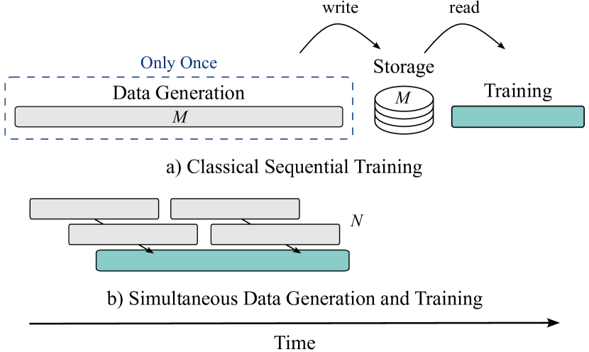
Figure 1: Classical I/O and storage intensive workflow for deep learning experiment (a) using $M$ samples presented several times through different epochs. (b) A file-free concurrent data generation and online training workflow processing $N$ samples. $N\gg M$.

3.1 Framework Overview

The framework is implemented as an extension of the open source project Melissa, initially designed to handle large-scale ensemble runs for sensitivity analysis (Terraz et al., 2017) and data assimilation (Friedemann & Raffin, 2022). The goal is to enable the online (no intermediate storage in files) training of a neural model from data generated through different simulation executions. These simulations are executed with different input parameters (parameter sweep), making the different members of the ensemble. We target executions on supercomputers where simulations can be large parallel solver codes executed on several nodes and the training parallelized on several GPUs. Compared to the original Melissa framework, the extension presented here provides deep learning support while addressing the specificities of online training, and implements new communication patterns.

The framework consists of three main elements: several clients, one server, and one launcher (Figure 2):

• The clients execute the same partial differential equations solver but each instance with a different set of parameters $\bm{\lambda}$. Once started, each client connects to the server and directly streams the generated data to the server.

• The server is in charge of the training. It receives data from connected clients. At any time, a subset of the entire data received so far is kept in a memory buffer. Batches are assembled from this memory buffer to feed the network. The server also chooses the set of parameters $\bm{\lambda}$ for each client to run, and forwards them to the launcher.

• The launcher orchestrates and monitors the execution. On supercomputers, it requests resource allocations to the machine job scheduler (e.g. Slurm (Yoo et al., 2003) or OAR (Capit et al., 2005)). On these allocations, the server starts first then the clients.

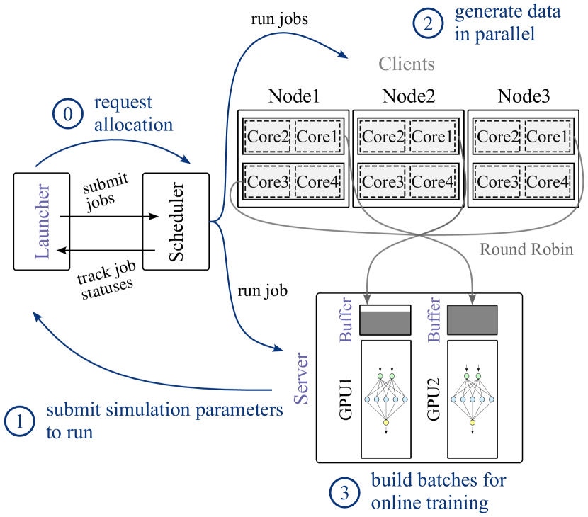
Figure 2: Framework architecture and workflow. The specific components introduced by the framework are colored in purple (e.g. the server). The different stages of the workflow are highlighted in blue. 2 and 3 occur simultaneously. In the depicted example, 6 clients run concurrently on 3 nodes. They are themselves parallelized on 2 cores. The training is performed in a data-distributed manner on 2 GPUs.

Appendix A provides details about the framework implementation.

3.2 Data Flow

The server can be executed on several GPUs, located or not on the same nodes, for data parallel training. Each GPU is associated with its own memory buffer of fixed size.

When a new client starts a simulation, it establishes connections with each of the server processes. As soon as the running simulation produces new data, they are sent to the server. Data are distributed between GPUs in a Round Robin fashion. No data are ever stored on disk, hence avoiding costly I/O operations.

The paper focuses on one-way data transfer. The clients transmit all the data required for training: the field of interest $u_{t}$ and possibly additional information the solver can provide like the adjoint. Nonetheless, the framework can also support bidirectional communications where the server communicates data back to the clients (Friedemann & Raffin, 2022). This is for instance necessary for applications based on backpropagation through the solver (Um et al., 2020; Rackauckas et al., 2020) or Deep RL for which updates of the policy network must be passed to the actors.

3.3 Data Management

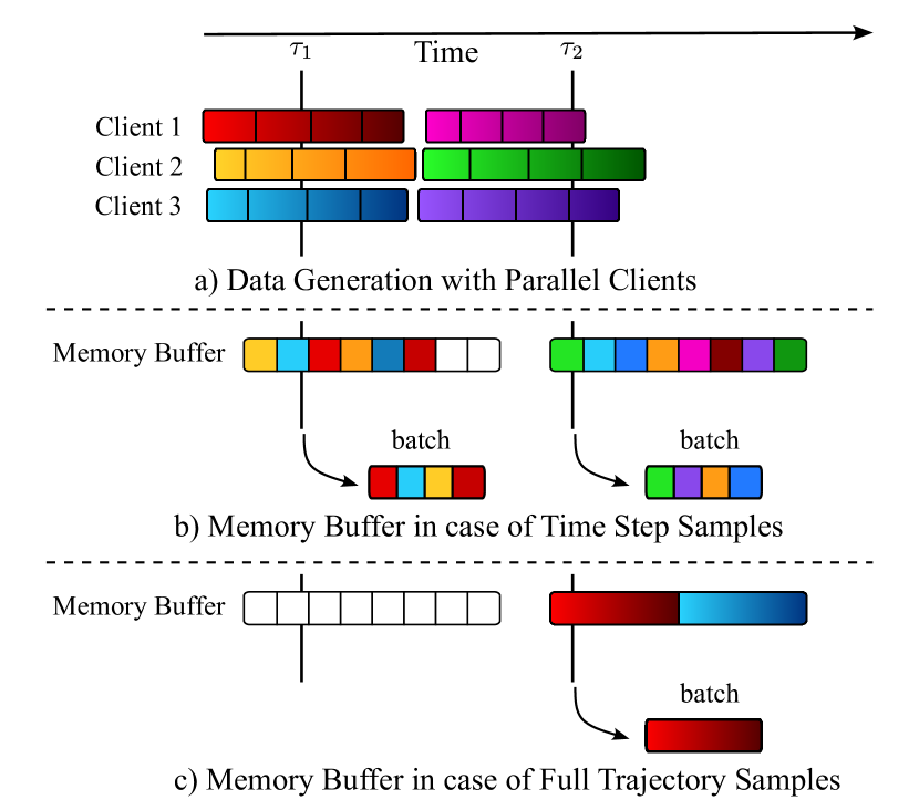
Figure 3: Flow of the generated simulation data. In a, 3 processes run 6 simulations in parallel. Groups of concurrent simulations are executed sequentially. In b, as soon as a simulation time step $u^{t}_{\lambda_{i}}$ is computed it is passed to the memory buffer. In c, the training requires access to the full trajectory and so the unit element in the buffer is a full trajectory. The content of the memory buffer is repesented a two different times $\tau_{1}$ and $\tau_{2}$. At time $\tau_{1}$ no batch can be extracted for c as no full trajectory is available yet.

Assembling batches with enough diversity is critical to apply stochastic gradient descent algorithm (Bottou et al., 2018). Biased batches can otherwise lead to catastrophic forgetting (Kemker et al., 2018) marked by decreased performances of the trained network.

The online training workflow comes with specific possible sources of bias:

• Intra-simulation bias: Solvers produce dynamics as time series by discretizing time and progressing iteratively. After $T$ time steps, only the data $u^{t}_{\lambda},0\leq t\leq T$ for the simulation parameter $\bm{\lambda}$ are available for training.

• Inter-simulation bias: Computational resources are limited and so often not all simulation instances can be executed concurrently. Let’s assume that only $c$ simulations can be executed concurrently at any time. At the end of the execution of the $c$ first simulations, training only has access to the data $u^{t}_{\lambda_{i}},0<i\leq c$.

• Memory bias: The set of data available for training is not only limited to the already generated data, it is further reduced due to memory constraints. At most, a rolling subset of the generated data that fits the given memory budget can be kept and used for training.

The management of the memory buffer is key to counteract these biases (Figure 3). Different management policies are available ranging from simple queues to reservoir sampling (Efraimidis & Spirakis, 2006). The one used in the experiments of this paper allows writing incoming data on free slots only, while each (random) read suppresses the corresponding data. So each data is seen only once during training. A watermark is also used to prevent the data loader from extracting samples from the buffer when too few are present. This also ensures bigger diversity in batches randomly taken from the buffer population.

The modality of training also impacts data management. The training may work with individual time steps, an interval of successive time steps or the full trajectory (Figure 3). Autoregressive models (Equation 5) require at least two successive time steps: the input and the target of the model. However, the implementation of the push forward trick introduced by Brandstetter et al. (2022) to stabilize long-term prediction of the network requires access to the full trajectory. This paper experiments with different situations. When the full trajectory is needed, the unit sample in the memory buffer encompasses the full trajectory.

The sampling strategy implemented by the server for selecting the parameters $\bm{\lambda}$ to run also has an impact on the inter-simulation bias. Classical Monte Carlo sampling is used throughout the paper. Nonetheless, the framework provides the abstraction to implement more advanced sampling strategies.

4 Experiments

The experiments consist in evaluating the performance of the framework in training state-of-the-art deep surrogate architectures on classical PDEs. Table 1 lists the different experiments, with the model that is trained, the equations ruling the use case, and the source of the model or solver. Except stated otherwise, the hyper-parameters of the training (e.g. the batch size) are kept identical to the original paper. Data generation details are provided in Appendix B. Experiments are run on NVIDIA V100 GPUs and Intel Xeon 2.5GHz processors. Table 2 synthesizes the experimental resources and the results obtained.

Table 1: Combinations of models and PDE use cases in the different experiments performed with the online training framework.

Experiment	PDE	Model	Source
E1	Heat equation	Fully Connected	—
E2	Lorenz’s system	Fully Connected	Lorenz (1963)
E3	Navier-Stokes	U-Net	Takamoto et al. (2022)
E4	Navier-Stokes	FNO	Li et al. (2021)
E5	Mixed Advection-Diffusion	Message Passing PDE Solver	Brandstetter et al. (2022)

Table 2: Comparison of the training modes for the different experiments. RESOURCES column indicates computing resources used for data generation.

Experiment	Resources	Generation (hours)	Total (hours)	Dataset (GB)	Unique Samples ($N$)	RMSE $\downarrow$	Gain (%)
E1 offline	10 cores	0.079	0.284	0.08	1e4	2.46	—
E1 online	10 cores	—	0.710	80.0	1e6	0.766	68.9
E3 offline	10 cores	3	3.82	0.328	1e3	0.1455	—
E3 online	1200 cores	—	6.39	328	5e5	0.1463	-0.549
E4 offline	10 cores	2.4	4.13	0.328	1e3	0.0876	—
E4 online	160 GPUs	—	3.95	328	5e5	0.0739	15.6
E5 offline	1 GPU	7.41	9.80	1.17	2.048e3	7.64	—
E5 online	400 Cores	—	2.50	82.4	4.96e5	7.18	6.02

4.1 Dataset Size Impact

A first motivational experiment examines the impact of the number of trajectories in the dataset on model performance in a classical offline training.

The Message Passing Neural PDE Solver is trained on the mixed advection-diffusion dataset consisting of a training set and a test set of respectively 2,048 and 128 trajectories as in Brandstetter et al. (2022). The trajectories differ only by the initial conditions of the PDE ($\bm{\lambda}=u_{0}$). Smaller training datasets are extracted from the original one. For each of these datasets, the model is always trained on 640,000 batches, and tested on the same test set. Table 3 shows the error decreases with the number of trajectories available.

Table 3: Test error of the Message Passing Neural PDE Solver trained on datasets of the mixed advection-diffusion with different numbers of training trajectories.

# Training Simulations	Size (MB)	RMSE $\downarrow$
409	240	4.13
1024	600	2.55
1638	960	2.13
2048	117	1.89

FNO is trained with 5 datasets of different sizes from the simple advection data. Trajectories differ by the initial conditions of the equation ($\bm{\lambda}=u_{0}$). We also test different training strategies combining an input of 1 or 10 consecutive time steps and a single time step or full rollout prediction. Figure 4 shows the error of the different trained models on the same test dataset of 100 unseen trajectories. All modalities benefit from larger datasets, except the history of 1 and full rollout that likely suffers from overfitting at 2000 trajectories. The benefit of a larger dataset is particularly noticeable when using the default configuration from (Li et al., 2021) (history of 10 and a full trajectory rollout) with a gain of $96\%$.

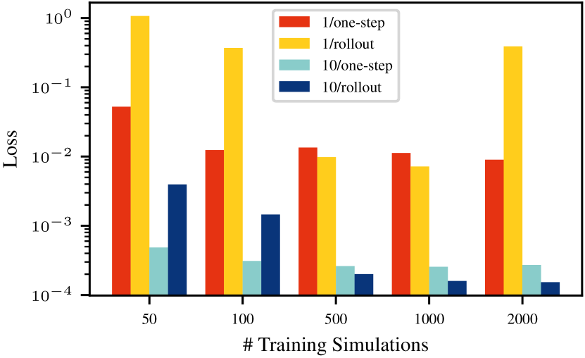
Figure 4: Test error of FNO trained on datasets of the simple advection with different numbers of trajectories. The different training strategies are noted history/rollout length.

The experiment shows that state-of-the-art models make lower errors in inference when trained on more trajectories. It corroborates similar results obtained for FNO on the Navier-Stokes equation (Li et al., 2021). Although the datasets considered presently are still relatively small (up to 1.6 GB), generating much more trajectories for training, which would help generalization, would soon be prohibitive in terms of memory. The framework proposed in the present article addresses this difficulty by avoiding writing any data on the disk.

4.2 Online Learning with Single Step Samples

The heat equation example (E1) trains a fully connected network to predict the entire 2D temperature field, given six temperature inputs: four boundary conditions, one initial condition, and the time step ($\bm{\lambda}=[u_{0},u_{\text{BC}}]$, each randomly sampled between 100K and 500K). The solver used to generate the data approximates the solution on a 100 x 100 spatial grid for 100 time steps representing 1 second. It relies on an implicit finite difference scheme. For the offline mode, two training datasets of respectively 100 and 500 trajectories are generated. The initial and boundary temperature conditions vary for each trajectory with values randomly selected between 100K and 500K. For the online mode, 1 node executes 5 clients to generate 10,000 trajectories. Each client runs the solver in parallel on 2 cores. Each time a new time step is completed, the 2D temperature field is sent to the memory buffer.

The model architecture consists of 3 layers of 1024 features, followed by ReLU activation function except for the output layer. The model performs direct prediction as described in Equation 4. Both online and offline training procedures follow the same learning rate schedule starting with a value of $1\text{E}^{-3}$ and decaying exponentially. For offline training, the number of epochs is adjusted to always train with 100,000 batches. The offline training dataset is repeated between epochs.

Figure 5 shows, for 5 repetitions of the experiment, the training and validation losses for the two offline training datasets and the online training. The mean is plotted in solid lines and bold colors. The online training presents more diversity to the network which is correlated with better generalization. The online example enables a deeper exploration of the problem resulting in about $70\%$ improved validation error compared to 100 simulations and 100 epochs offline. Additionally, the gap between the decreasing training loss and the plateaued validation loss of the model trained in the offline settings is symptomatic of overfitting. The model trained with the online framework is less prone to such overfitting.

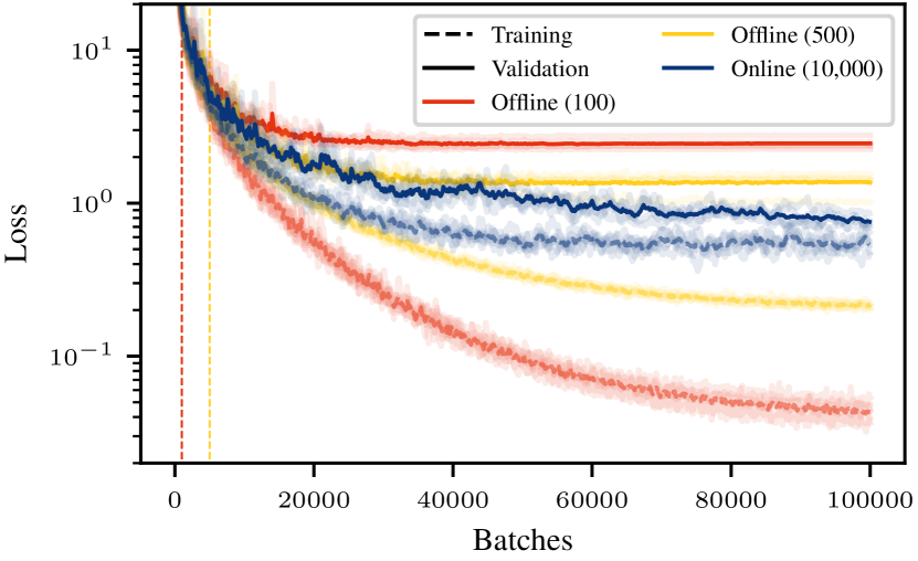
Figure 5: Comparison of the online and offline training on the Heat Equation (E1). Solid lines represent the mean values of five realizations. Vertical lines represent the first epoch of the corresponding offline training, after which the dataset is repeated while the online setting always processes new data.

In the example of the Lorenz’s system (E2) the goal is to train a fully connected autoregressive model composed of 3 layers of 512 features followed by SiLU activation to recover the chaotic dynamics of the system. The model takes as input $\rho$, the parameter of the equation that varies across the simulations, and $X_{t}$ the position at the current time step ($\bm{\lambda}=[u_{0},\rho]$). It predicts the next position $X_{t+\delta t}$. The trajectory generation is detailed in Section B.2. Three different offline training datasets are used for the experiment. They respectively count 100, 10 and 10,000 trajectories. The trajectories of the latter are subsampled every 100 time steps. 10 and 10,000 datasets are symbolic of more complex systems for which storage limitations impose a scarcity of data. For each dataset, the model is trained for 100, 1000, and 100 epochs respectively. For the online dataset, we generate 10000 trajectories. The $u_{0}$ parameter is randomly sampled. In the streaming online training, the memory buffer is a simple FIFO queue and the trajectories are generated from simulations with increasing values of $\rho$, creating an inter-simulation bias not altered by the FIFO queue. The Sampling + Buffer online training randomly samples $\rho$ and uses the default memory buffer introduced in Section 3.3. For all training strategies, the batch size is 1024. The validation dataset consists of 10 trajectories.

Figure 6 shows the training dynamics for the different offline and online settings. The offline training with 10 trajectories and the one with 10,000 subsampled trajectories present signs of overfitting, indicating that more data are necessary to properly capture the chaotic dynamic of the system. Online training with 10,000 performs as well as offline training with 100 trajectories over 100 epochs. The streaming training presents the worse validation curve which can be explained by catastrophic forgetting (Kemker et al., 2018). These results highlight the importance of the bias mitigation strategy and the ability of the framework to outperform classical training with scarce data. The efficiency of the bias mitigation strategy from the perspective of the batch statistics is further discussed in Appendix C.

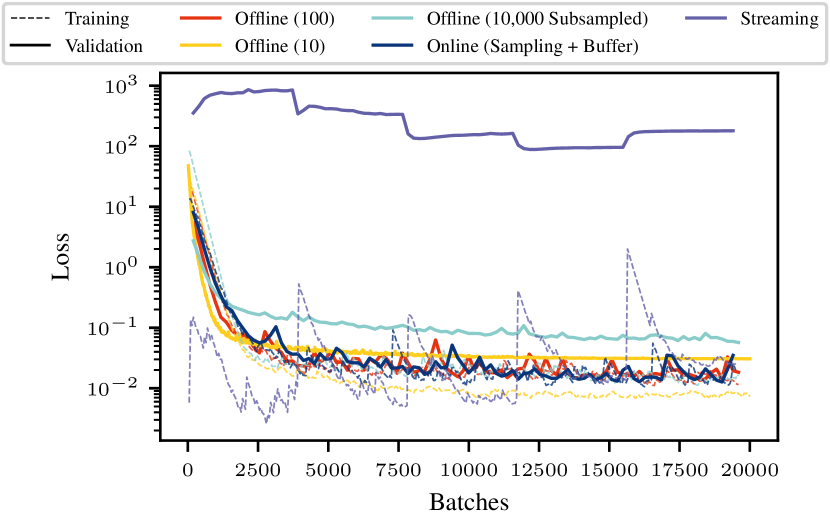
Figure 6: Comparison between the training and validation losses for different training strategies on the Lorenz’s system (E2).

4.3 Online Training on Full Trajectories

This subsection focuses on the online training of FNO (E4), U-Net (E3), and Message Passing Neural PDE Solver (E5).

The FNO (in its 2-D version) and U-Net architectures are trained on a use case ruled by the Navier-Stokes equations, as in Li et al. (2021); Takamoto et al. (2022). For the offline mode, the training dataset consists of 1,000 trajectories repeated over 500 epochs with a batch size of 20 ($\bm{\lambda}=u_{0}$). For the online mode, data generation is either performed on 30 nodes of 40 cores each, or on 40 nodes of 4 GPUs each (in this case clients run on GPU). This allows running 31,250 clients each generating 16 trajectories for a total of 500,000 simulations. The same validation dataset is used to evaluate the performance of both training sessions. It consists of 200 trajectories generated offline. Both FNO and U-Net architectures are trained as autoregressive models following the original procedure (Li et al., 2021).

Figure 7 compares the training and validation loss for the two architectures and for the two different ways of training. Each experiment was repeated five times. For the U-Net architecture, the online framework leads to similar results to offline training after 15,000 batches. On average, performances are similar but the online training is characterized by strong variations around the mean value. This instability echoes the observations of Takamoto et al. (2022), where the so called pushforward trick was used to stabilize the architecture. On the other hand, the online framework has a clear positive impact on the performance of FNO, which outperforms U-Net. Online training is indeed characterized by a lower validation loss compared to offline training.

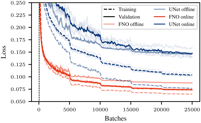
Figure 7: Comparison between the offline and online training of the FNO and U-Net architectures on the Navier-Stokes Equations (E3,E4). The vertical line represents the first epoch accounting for 50 batches of 20 full trajectories each.

The experiment E5 tests the impact of the online training framework on the Message Passing PDE Solver with the use case of the mixed advection-diffusion ($\bm{\lambda}=[u_{0},\alpha,\beta,\gamma]$). The solver generates trajectories by groups of 4. The equation parameters $\alpha$, $\beta$, and $\gamma$ vary from one group to another. Only the initial conditions vary within a group. For offline data generation, the solver is used as it is. For the online mode, it is only modified to send the data to the server relying on the framework API, instead of writing the data on disk. The offline training dataset consists of 2,048 trajectories. The model is trained for 20 epochs. The online data generation is performed over 10 nodes of 40 cores each. It executes sequentially two ensembles of 400 clients. Each client generates 128 batches of 4 simulations. In total, online data generation produces 409,600 trajectories. Online training is achieved on 2 GPUs (data parallelism). Clients feed iteratively each memory buffer associated with each GPU in a Round Robin fashion. Both training methods are validated on the same dataset consisting of 128 trajectories.

Figure 8 compares the training and validation losses. Online training presents an almost constantly lower validation loss. Evaluation on a test set shows that training the model with the online framework improves the performance by 7% compared to the offline training.

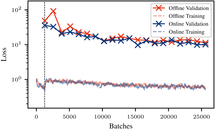
Figure 8: Comparison between the offline and online training of the Message Passing PDE Server on the mixed advection-diffusion (E5). The vertical line represents the limit of the first epoch.

Section 4.1 showed that, offline, bigger datasets generally improve surrogate model performances. The different online experiments indicate the framework sustains this trend despite the online setting. During training, it exposes the model to more unique samples which results in better generalization compared to offline training for the same number of processed batches. The different experiments also exhibit the versatility of the framework. Several models are trained on multiple PDE use cases. Several degrees of parallelism are presented for the data generation.

5 Conclusion

Deep surrogate models are promising candidates to accelerate the numerical simulations of PDEs, unlocking faster engineering processes and further scientific discoveries. The proposed online training framework leverages HPC resources to expose these models to bigger datasets, with more diverse trajectories, than it would otherwise be possible with classical offline training, due to I/O and storage limitations. By relying on simple techniques like a memory buffer and Monte Carlo sampling, the framework mitigates the inherent bias of streaming learning. Our framework enabled to process online datasets up to 328 GB and improve the generalization of fully connected neural networks by 68%, FNO by 16%, and Message Passing PDE Solver by 7%. In future work, such improvement could be further enhanced by relying on active learning.

Appendix A Framework Details

A.1 Implementation

The framework is mainly implemented in Python. The server supports data parallel training for Pytorch and Tensorflow models. Supporting an existing parallel solver (MPI+X parallelization supported) requires 1) instrumenting the code to call the API (for C, C++, Fortran or Python) enabling to connect and ship the data to the server, 2) instructing the server on how to perform the training and 3) defining the experimental design, i.e. how to draw the input parameter set for each instance.

This paper focuses on full online training, but the framework can start from a pre-trained model, and data provided for training can mix some read from files using a proxy client. This enables to reduce repetitive data generation during the hyper-parameterization process.

Communications are implemented with ZeroMQ (Hintjens, 2013). ZeroMQ manages asynchronous data transfers, stored when necessary in internal buffers on the client and server sides to absorb network variability. If these buffers fill up the simulation is suspended. On the server side a thread associated to each GPU is dedicated to data reception and insertion into the memory buffer. Data formatting occurs at this stage when required. Another thread builds batches from the content of the buffer and trains the model with them.

A.2 Fault Tolerance

The framework is designed for application on large clusters. It is made resilient to different faults that can occur on such infrastructure. Failing clients are automatically restarted. The server keeps track of the received time steps $u_{\lambda}^{t}$ and discards already received ones. If the server fails, it is restarted with all the running clients. In case of launcher failure, the currently running clients will run up to completion and the server will finish and checkpoint. A manual restart of the full application is then needed to restart from that checkpoint. The scheduler of the cluster (e.g. Slurm (Yoo et al., 2003)) comes with its own fault tolerance mechanism. A failing request of the scheduler is simply resubmitted later.

A.3 Reproducibility

The stochastic components of the framework (the model’s weights initialization, the simulation parameter sampler, and the buffer policy) are seeded. The framework operates with configuration files which also contributes to the reproducibility of training experiments. However, the distributed execution on a cluster comes with inevitable variability which makes identical reproducibility challenging. Indeed, the execution of the clients is subject to the workload of the cluster, which impacts the order of the data received by the server and may ultimately lead to variations in the training.

Appendix B Equations

B.1 The Heat Equation

Equation 6 describes the evolution of the temperature $u$ in a 2D square domain of length $L$. $\alpha$ represents the thermal diffusivity of the medium. The system is fully determined by initial conditions (Equation 7) and boundary conditions (Equation 8). The solver used to generate the training data approximates the solution with an implicit Euler scheme of finite difference. It solves the equation on a $100\times 100$ regular grid, with time steps of $0.01$s for a total simulated time of $1$s. The thermal diffusivity is fixed, $\alpha=1\ \text{m}^{2}\cdot\text{s}^{-1}$. The initial temperature is considered uniform over the domain, while the temperatures at the edge of the domain are constant but not necessarily equal. All temperature conditions take random values in $[100\text{K},500\text{K}]$.

$$\frac{\partial u}{\partial t}=\alpha\Delta u$$ (6)

$$u(x,y,t=0)=T_{\text{IC}}$$ (7)

$$u(x=0,y,t)=T_{x_{1}},\ u(x=L,y,t)=T_{x_{2}}$$

$$u(x,y=0,t)=T_{y_{1}},\ u(x,y=L,t)=T_{y_{2}}$$ (8)

B.2 The Lorenz’s System

LABEL:eq:lorenz describes the famous chaotic system introduced by Lorenz that serves as a simplified climate model (Lorenz, 1963). An explicit Euler integration scheme allows the recovery of the trajectory of the system given an initial position. It approximates the solution with time steps of $0.01$s for a total simulated time of $20$s. For the dataset generation, the parameters $\sigma$ and $\beta$ are fixed to the respective values of $10$ and $8/3$. The initial position of each trajectory is randomly taken according to the normal distribution $\mathcal{N}(15,30)$. $\rho$ takes values in $[0,20,40,60,80,100]$.

$$\frac{dx}{dt} =\sigma(y-z)$$

$$\frac{dy}{dt} =x(\rho-z)-y$$

$$\frac{dz}{dt} =xy-\beta z$$

B.3 Simple Advection

The Advection is a standard example of PDEs. The implementation of the example is directly taken from the PDEBench paper (Takamoto et al., 2022) §D.1.

B.4 Mixed Advection-Diffusion

The Advection-Diffusion considers a combination of phenomena: the simple advection, and the diffusion of a quantity $u$. The implementation of the example is directly taken from the original paper of the Message Passing PDE Solver (Brandstetter et al., 2022) experiment E3 in §4.1.

B.5 The Navier-Stokes Equations

The Navier-Stokes equations are canonical to describe the evolution of any fluid (Ferziger et al., 2002). Equation 10, 11 and 12 describe the evolution of a 2D incompressible fluid on the surface of the unit torus, in terms of velocity $u$, and vorticity $w$ where $w=\nabla\times u$. $\nu$ denotes the viscosity of the fluid. It is set to $1\text{E}^{-5}\text{m}^{2}\cdot\text{s}^{-1}$. $f$ denotes the forcing term of the system. The equations are solved with a pseudo-spectral method for $(x,t)\in[0,1]^{2}\times[0,T]$ and periodic boundary conditions. The equations are discretized on a 64 x 64 regular mesh, with a time step of $1\text{E}^{-4}s$ for a total simulated time of $20$s. The solver generating the training data is the same as for the original paper of FNO (Li et al., 2021).

$$\partial_{t}w(x,t)+u(x,t)\cdot\nabla w(c,t)=\nu\Delta w(x,t)+f(x)$$ (10)

$$\nabla\cdot u(x,t)=0$$ (11)

$$w(x,t=0)=w_{0}(x)$$ (12)

Appendix C Bias Mitigation

The online setting of the framework inherently induces biases in the data available for training (Section 3.3). The efficiency of the bias mitigation strategy consisting of Monte Carlo sampling of the simulation parameters and mixing of the received data within the memory buffer is evaluated on the Lorenz’s system described in Section B.2. Figure 9 compares the batch statistics of the normalized inputs for different training settings identical to the ones presented in Section 4.2. $\rho$ is normalized between $0$ and $1$, using minimum and maximum values. Coordinates $x$, $y$, and $z$ are standardized. The Offline (100) corresponds to classical offline training with data sampled randomly from 100 previously generated trajectories. The sampling being uniform, the batches present an almost constant mean and standard deviation. It is assumed that representative and well-balanced batches with constant statistics will lead to faster stochastic gradient descent convergence and better generalization capabilities of the trained model. Streaming refers to the case where trajectories are generated by order of increasing $\rho$ and batches are formed with data as soon as they are received by the server. Figure 9 highlights batch statistics are biased towards the simulation that has just been executed. For the online sampling, the parameter $\rho$ is randomly sampled. It immediately improves the fluctuations of batch statistics. The addition of the memory buffer further improves the batch statistics making them closer to the ones observed in the offline setting.

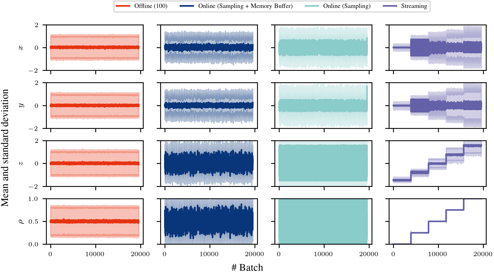
Figure 9: Statistics of the normalized inputs for the Lorenz’s system (E2) with different bias mitigation strategies.

Appendix D Prediction Results

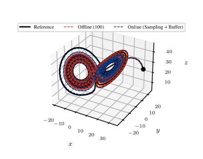
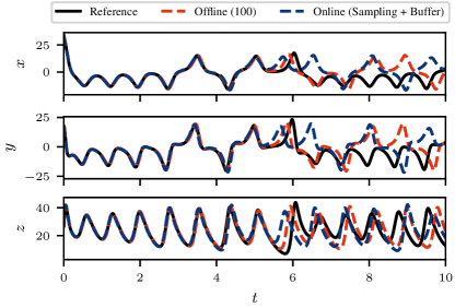
Figure 10: Comparison of the predictions for the Lorenz’s system and a trajectory never seen during training with $\rho=28$.

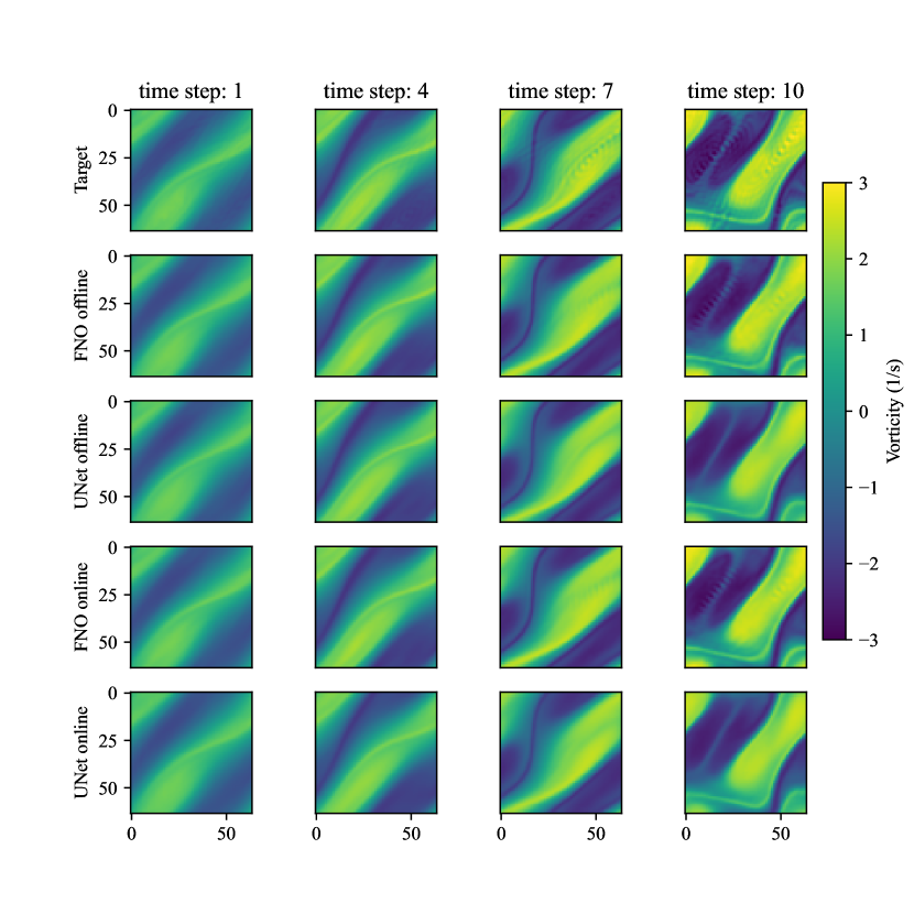
Figure 11: Visual comparison of Navier-Stokes predictions from U-Net and FNO

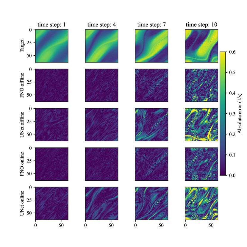
Figure 12: Visual comparison of Navier-Stokes prediction error from U-Net and FNO

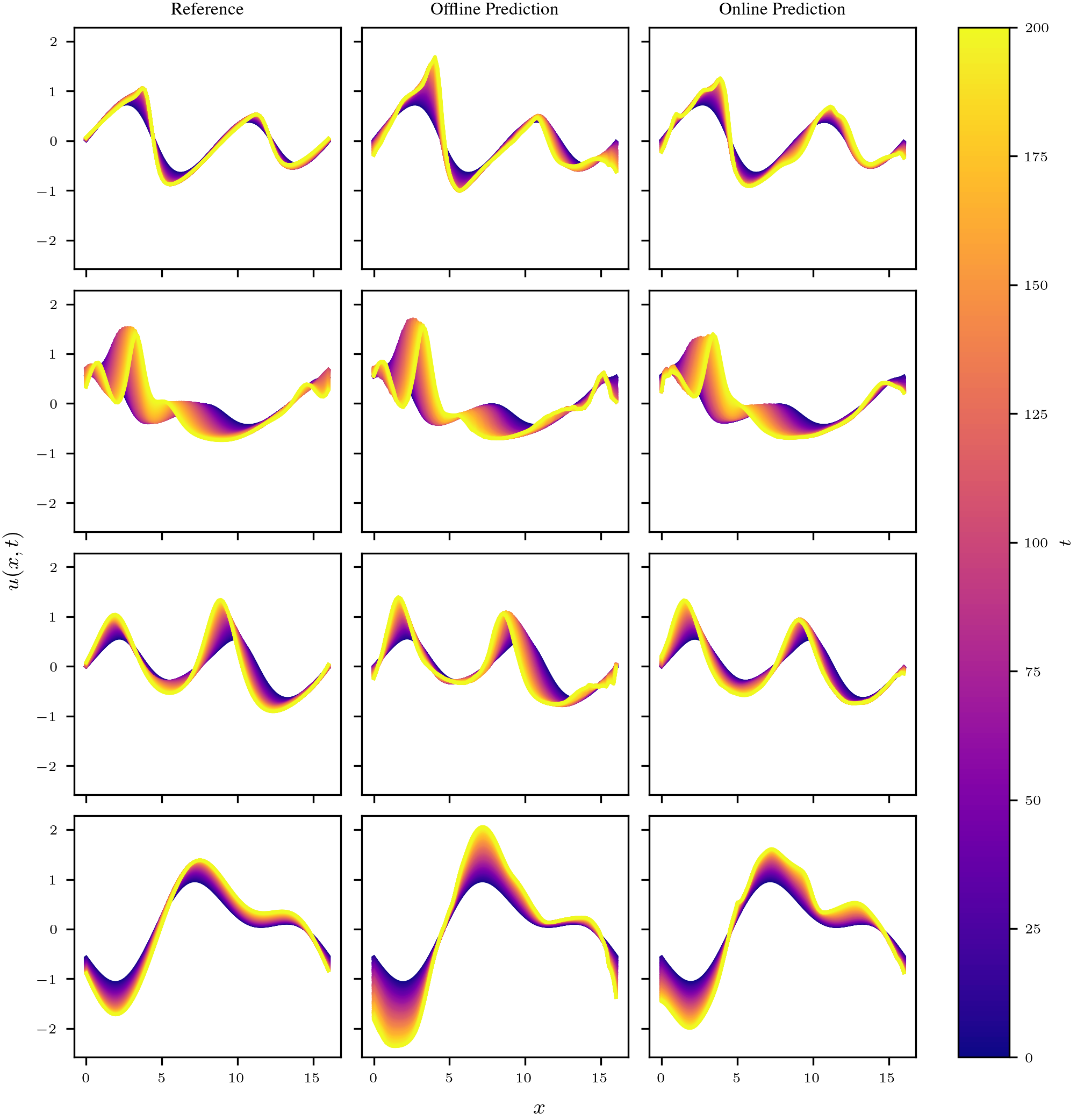
Figure 13: Visual comparison of Message Passing PDE Solver predictions on mixed advection-diffusion

References

- Berner et al. (2019) Berner, C., Brockman, G., Chan, B., Cheung, V., Dębiak, P., Dennison, C., Farhi, D., Fischer, Q., Hashme, S., Hesse, C., et al. Dota 2 with large scale deep reinforcement learning. ArXiv preprint, abs/1912.06680, 2019.
- Bonnet et al. (2022) Bonnet, F., Mazari, J. A., Cinnella, P., and Gallinari, P. AirfRANS: High fidelity computational fluid dynamics dataset for approximating reynolds-averaged navier–stokes solutions. In Thirty-sixth Conference on Neural Information Processing Systems Datasets and Benchmarks Track, 2022.
- Bottou et al. (2018) Bottou, L., Curtis, F. E., and Nocedal, J. Optimization methods for large-scale machine learning. Siam Review, 60(2):223–311, 2018.
- Brace et al. (2022) Brace, A., Yakushin, I., Ma, H., Trifan, A., Munson, T., Foster, I., Ramanathan, A., Lee, H., Turilli, M., and Jha, S. Coupling streaming ai and hpc ensembles to achieve 100–1000 faster biomolecular simulations. In 2022 IEEE International Parallel and Distributed Processing Symposium (IPDPS), pp. 806–816. IEEE, 2022.
- Brandstetter et al. (2022) Brandstetter, J., Worrall, D. E., and Welling, M. Message passing neural PDE solvers. In The Tenth International Conference on Learning Representations, ICLR 2022, Virtual Event, April 25-29, 2022, 2022.
- Brown et al. (2020) Brown, T. B., Mann, B., Ryder, N., Subbiah, M., Kaplan, J., Dhariwal, P., Neelakantan, A., Shyam, P., Sastry, G., Askell, A., Agarwal, S., Herbert-Voss, A., Krueger, G., Henighan, T., Child, R., Ramesh, A., Ziegler, D. M., Wu, J., Winter, C., Hesse, C., Chen, M., Sigler, E., Litwin, M., Gray, S., Chess, B., Clark, J., Berner, C., McCandlish, S., Radford, A., Sutskever, I., and Amodei, D. Language models are few-shot learners. In Larochelle, H., Ranzato, M., Hadsell, R., Balcan, M., and Lin, H. (eds.), Advances in Neural Information Processing Systems 33: Annual Conference on Neural Information Processing Systems 2020, NeurIPS 2020, December 6-12, 2020, virtual, 2020.
- Brunton et al. (2020) Brunton, S. L., Noack, B. R., and Koumoutsakos, P. Machine learning for fluid mechanics. Annual review of fluid mechanics, 52:477–508, 2020.
- Burden et al. (2015) Burden, R. L., Faires, J. D., and Burden, A. M. Numerical analysis. Cengage learning, 2015.
- Capit et al. (2005) Capit, N., Da Costa, G., Georgiou, Y., Huard, G., Martin, C., Mounié, G., Neyron, P., and Richard, O. A batch scheduler with high level components. In CCGrid 2005. IEEE International Symposium on Cluster Computing and the Grid, 2005., volume 2, pp. 776–783. IEEE, 2005.
- Chakraborty (2021) Chakraborty, S. Transfer learning based multi-fidelity physics informed deep neural network. Journal of Computational Physics, 426:109942, 2021.
- Efraimidis & Spirakis (2006) Efraimidis, P. S. and Spirakis, P. G. Weighted random sampling with a reservoir. Information processing letters, 97(5):181–185, 2006.
- Espeholt et al. (2018) Espeholt, L., Soyer, H., Munos, R., Simonyan, K., Mnih, V., Ward, T., Doron, Y., Firoiu, V., Harley, T., Dunning, I., Legg, S., and Kavukcuoglu, K. IMPALA: scalable distributed deep-rl with importance weighted actor-learner architectures. In Dy, J. G. and Krause, A. (eds.), Proceedings of the 35th International Conference on Machine Learning, ICML 2018, Stockholmsmässan, Stockholm, Sweden, July 10-15, 2018, volume 80 of Proceedings of Machine Learning Research, pp. 1406–1415. PMLR, 2018.
- Ferziger et al. (2002) Ferziger, J. H., Perić, M., and Street, R. L. Computational methods for fluid dynamics, volume 3. Springer, 2002.
- Friedemann & Raffin (2022) Friedemann, S. and Raffin, B. An elastic framework for ensemble-based large-scale data assimilation. The international journal of high performance computing applications, 36(4):543–563, 2022.
- Hennigh et al. (2021) Hennigh, O., Narasimhan, S., Nabian, M. A., Subramaniam, A., Tangsali, K., Fang, Z., Rietmann, M., Byeon, W., and Choudhry, S. Nvidia simnet™: An ai-accelerated multi-physics simulation framework. In International Conference on Computational Science, pp. 447–461. Springer, 2021.
- Hintjens (2013) Hintjens, P. ZeroMQ: messaging for many applications. " O’Reilly Media, Inc.", 2013.
- Horgan et al. (2018) Horgan, D., Quan, J., Budden, D., Barth-Maron, G., Hessel, M., van Hasselt, H., and Silver, D. Distributed prioritized experience replay. In 6th International Conference on Learning Representations, ICLR 2018, Vancouver, BC, Canada, April 30 - May 3, 2018, Conference Track Proceedings, 2018.
- Karniadakis et al. (2021) Karniadakis, G. E., Kevrekidis, I. G., Lu, L., Perdikaris, P., Wang, S., and Yang, L. Physics-informed machine learning. Nature Reviews Physics, 3(6):422–440, 2021.
- Kemker et al. (2018) Kemker, R., McClure, M., Abitino, A., Hayes, T. L., and Kanan, C. Measuring catastrophic forgetting in neural networks. In McIlraith, S. A. and Weinberger, K. Q. (eds.), Proceedings of the Thirty-Second AAAI Conference on Artificial Intelligence, (AAAI-18), the 30th innovative Applications of Artificial Intelligence (IAAI-18), and the 8th AAAI Symposium on Educational Advances in Artificial Intelligence (EAAI-18), New Orleans, Louisiana, USA, February 2-7, 2018, pp. 3390–3398. AAAI Press, 2018.
- Kochkov et al. (2021) Kochkov, D., Smith, J. A., Alieva, A., Wang, Q., Brenner, M. P., and Hoyer, S. Machine learning–accelerated computational fluid dynamics. Proceedings of the National Academy of Sciences, 118(21):e2101784118, 2021.
- Krishnapriyan et al. (2021) Krishnapriyan, A. S., Gholami, A., Zhe, S., Kirby, R. M., and Mahoney, M. W. Characterizing possible failure modes in physics-informed neural networks. In Ranzato, M., Beygelzimer, A., Dauphin, Y. N., Liang, P., and Vaughan, J. W. (eds.), Advances in Neural Information Processing Systems 34: Annual Conference on Neural Information Processing Systems 2021, NeurIPS 2021, December 6-14, 2021, virtual, pp. 26548–26560, 2021.
- Lee et al. (2021) Lee, H., Merzky, A., Tan, L., Titov, M., Turilli, M., Alfe, D., Bhati, A., Brace, A., Clyde, A., Coveney, P., et al. Scalable hpc & ai infrastructure for covid-19 therapeutics. In Proceedings of the Platform for Advanced Scientific Computing Conference, pp. 1–13, 2021.
- Li et al. (2020) Li, S., Zhao, Y., Varma, R., Salpekar, O., Noordhuis, P., Li, T., Paszke, A., Smith, J., Vaughan, B., Damania, P., et al. Pytorch distributed: Experiences on accelerating data parallel training. Proceedings of the VLDB Endowment, 13(12), 2020.
- Li et al. (2021) Li, Z., Kovachki, N. B., Azizzadenesheli, K., Liu, B., Bhattacharya, K., Stuart, A. M., and Anandkumar, A. Fourier neural operator for parametric partial differential equations. In 9th International Conference on Learning Representations, ICLR 2021, Virtual Event, Austria, May 3-7, 2021, 2021.
- Liang et al. (2018) Liang, E., Liaw, R., Nishihara, R., Moritz, P., Fox, R., Goldberg, K., Gonzalez, J., Jordan, M. I., and Stoica, I. Rllib: Abstractions for distributed reinforcement learning. In Dy, J. G. and Krause, A. (eds.), Proceedings of the 35th International Conference on Machine Learning, ICML 2018, Stockholmsmässan, Stockholm, Sweden, July 10-15, 2018, volume 80 of Proceedings of Machine Learning Research, pp. 3059–3068. PMLR, 2018.
- Lorenz (1963) Lorenz, E. N. Deterministic nonperiodic flow. Journal of atmospheric sciences, 20(2):130–141, 1963.
- Lu et al. (2021) Lu, L., Jin, P., Pang, G., Zhang, Z., and Karniadakis, G. E. Learning nonlinear operators via deeponet based on the universal approximation theorem of operators. Nature Machine Intelligence, 3(3):218–229, 2021.
- Lucor et al. (2022) Lucor, D., Agrawal, A., and Sergent, A. Simple computational strategies for more effective physics-informed neural networks modeling of turbulent natural convection. Journal of Computational Physics, 456:111022, 2022.
- Merity et al. (2017) Merity, S., Xiong, C., Bradbury, J., and Socher, R. Pointer sentinel mixture models. In 5th International Conference on Learning Representations, ICLR 2017, Toulon, France, April 24-26, 2017, Conference Track Proceedings, 2017.
- Otness et al. (2021) Otness, K., Gjoka, A., Bruna, J., Panozzo, D., Peherstorfer, B., Schneider, T., and Zorin, D. An extensible benchmark suite for learning to simulate physical systems. In Thirty-fifth Conference on Neural Information Processing Systems Datasets and Benchmarks Track (Round 1), 2021.
- Peterson et al. (2022) Peterson, J. L., Bay, B., Koning, J., Robinson, P., Semler, J., White, J., Anirudh, R., Athey, K., Bremer, P.-T., Di Natale, F., et al. Enabling machine learning-ready hpc ensembles with merlin. Future Generation Computer Systems, 131:255–268, 2022.
- Pfaff et al. (2021) Pfaff, T., Fortunato, M., Sanchez-Gonzalez, A., and Battaglia, P. W. Learning mesh-based simulation with graph networks. In 9th International Conference on Learning Representations, ICLR 2021, Virtual Event, Austria, May 3-7, 2021, 2021.
- Rackauckas et al. (2020) Rackauckas, C., Ma, Y., Martensen, J., Warner, C., Zubov, K., Supekar, R., Skinner, D., Ramadhan, A., and Edelman, A. Universal differential equations for scientific machine learning. ArXiv preprint, abs/2001.04385, 2020.
- Raissi et al. (2019) Raissi, M., Perdikaris, P., and Karniadakis, G. E. Physics-informed neural networks: A deep learning framework for solving forward and inverse problems involving nonlinear partial differential equations. Journal of Computational physics, 378:686–707, 2019.
- Raissi et al. (2020) Raissi, M., Yazdani, A., and Karniadakis, G. E. Hidden fluid mechanics: Learning velocity and pressure fields from flow visualizations. Science, 367(6481):1026–1030, 2020.
- Ren et al. (2021) Ren, P., Xiao, Y., Chang, X., Huang, P.-Y., Li, Z., Gupta, B. B., Chen, X., and Wang, X. A survey of deep active learning. ACM computing surveys (CSUR), 54(9):1–40, 2021.
- Ribés et al. (2022) Ribés, A., Terraz, T., Fournier, Y., Iooss, B., and Raffin, B. Unlocking Large Scale Uncertainty Quantification with In Transit Iterative Statistics, pp. 113–136. Springer International Publishing, Cham, 2022. ISBN 978-3-030-81627-8.
- Ronneberger et al. (2015) Ronneberger, O., Fischer, P., and Brox, T. U-net: Convolutional networks for biomedical image segmentation. In International Conference on Medical image computing and computer-assisted intervention, pp. 234–241. Springer, 2015.
- Russakovsky et al. (2015) Russakovsky, O., Deng, J., Su, H., Krause, J., Satheesh, S., Ma, S., Huang, Z., Karpathy, A., Khosla, A., Bernstein, M., et al. Imagenet large scale visual recognition challenge. International journal of computer vision, 115(3):211–252, 2015.
- Satorras et al. (2021) Satorras, V. G., Hoogeboom, E., and Welling, M. E(n) equivariant graph neural networks. In Meila, M. and Zhang, T. (eds.), Proceedings of the 38th International Conference on Machine Learning, ICML 2021, 18-24 July 2021, Virtual Event, volume 139 of Proceedings of Machine Learning Research, pp. 9323–9332. PMLR, 2021.
- Sergeev & Del Balso (2018) Sergeev, A. and Del Balso, M. Horovod: fast and easy distributed deep learning in tensorflow. ArXiv preprint, abs/1802.05799, 2018.
- Sirignano & Spiliopoulos (2018) Sirignano, J. and Spiliopoulos, K. Dgm: A deep learning algorithm for solving partial differential equations. Journal of computational physics, 375:1339–1364, 2018.
- Stevens et al. (2020) Stevens, R., Taylor, V., Nichols, J., Maccabe, A. B., Yelick, K., and Brown, D. Ai for science: Report on the department of energy (doe) town halls on artificial intelligence (ai) for science. Technical report, Argonne National Lab.(ANL), Argonne, IL (United States), 2020.
- Stiller et al. (2022) Stiller, P., Makdani, V., Pöschel, F., Pausch, R., Debus, A., Bussmann, M., and Hoffmann, N. Continual learning autoencoder training for a particle-in-cell simulation via streaming. ArXiv preprint, abs/2211.04770, 2022.
- Takamoto et al. (2022) Takamoto, M., Praditia, T., Leiteritz, R., MacKinlay, D., Alesiani, F., Pflüger, D., and Niepert, M. Pdebench: An extensive benchmark for scientific machine learning. In Thirty-sixth Conference on Neural Information Processing Systems Datasets and Benchmarks Track, 2022.
- Terraz et al. (2017) Terraz, T., Ribes, A., Fournier, Y., Iooss, B., and Raffin, B. Melissa: large scale in transit sensitivity analysis avoiding intermediate files. In Proceedings of the international conference for high performance computing, networking, storage and analysis, pp. 1–14, 2017.
- Um et al. (2020) Um, K., Brand, R., Fei, Y. R., Holl, P., and Thuerey, N. Solver-in-the-loop: Learning from differentiable physics to interact with iterative pde-solvers. In Larochelle, H., Ranzato, M., Hadsell, R., Balcan, M., and Lin, H. (eds.), Advances in Neural Information Processing Systems 33: Annual Conference on Neural Information Processing Systems 2020, NeurIPS 2020, December 6-12, 2020, virtual, 2020.
- Wandel et al. (2021) Wandel, N., Weinmann, M., and Klein, R. Learning incompressible fluid dynamics from scratch - towards fast, differentiable fluid models that generalize. In 9th International Conference on Learning Representations, ICLR 2021, Virtual Event, Austria, May 3-7, 2021, 2021.
- Wang et al. (2020) Wang, R., Kashinath, K., Mustafa, M., Albert, A., and Yu, R. Towards physics-informed deep learning for turbulent flow prediction. In Gupta, R., Liu, Y., Tang, J., and Prakash, B. A. (eds.), KDD ’20: The 26th ACM SIGKDD Conference on Knowledge Discovery and Data Mining, Virtual Event, CA, USA, August 23-27, 2020, pp. 1457–1466. ACM, 2020.
- Yoo et al. (2003) Yoo, A. B., Jette, M. A., and Grondona, M. Slurm: Simple linux utility for resource management. In Workshop on job scheduling strategies for parallel processing, pp. 44–60. Springer, 2003.
- You et al. (2020) You, Y., Li, J., Reddi, S. J., Hseu, J., Kumar, S., Bhojanapalli, S., Song, X., Demmel, J., Keutzer, K., and Hsieh, C. Large batch optimization for deep learning: Training BERT in 76 minutes. In 8th International Conference on Learning Representations, ICLR 2020, Addis Ababa, Ethiopia, April 26-30, 2020, 2020.