Forward-backward algorithm for functions with locally Lipschitz gradient: applications to mean field games.

Abstract

In this paper, we provide a generalization of the forward-backward splitting algorithm for minimizing the sum of a proper convex lower semicontinuous function and a differentiable convex function whose gradient satisfies a locally Lipschitz-type condition. We prove the convergence of our method and derive a linear convergence rate when the differentiable function is locally strongly convex. We recover classical results in the case when the gradient of the differentiable function is globally Lipschitz continuous and an already known linear convergence rate when the function is globally strongly convex. We apply the algorithm to approximate equilibria of variational mean field game systems with local couplings. Compared with some benchmark algorithms to solve these problems, our numerical tests show similar performances in terms of the number of iterations but an important gain in the required computational time.

MSC Classification]65K05, 90C25, 90C90, 91-08, 91A16, 49N80, 35Q89.

1 Introduction

In this paper, we aim to solve the following problem.

Problem 1.

Let ${\mathcal{H}}$ be a real Hilbert space, let $\psi\colon{\mathcal{H}}\to\left]-\infty,+\infty\right]$ be a proper lower semicontinuous convex function, and let $\varphi\colon{\mathcal{H}}\to\mathbb{R}$ be a convex Gâteaux differentiable function such that, for every $x\in{\mathcal{H}}$ and every $M\in\left]0,+\infty\right[$, there exist $\mu_{M}(x)\in\left[0,+\infty\right[$ and $L_{M}(x)\in\left[\mu_{M}(x),{+\infty}\right[$ such that, for all $y,z\in B_{M}(x)$,

$$\mu_{M}(x)\|y-z\|^{2}\leq{\left\langle{{y-z}\mid{\nabla\varphi(y)-\nabla\varphi(z)}}\right\rangle}\leq L_{M}(x)\|y-z\|^{2},$$ (1)

where $B_{M}(x)$ is the open ball centered at $x$ with radius $M$. The problem is to

$$\underset{\begin{subarray}{c}{x\in{\mathcal{H}}}\end{subarray}}{\text{\rm minimize}}\;\;\psi(x)+\varphi(x),$$ (2)

under the assumption that the set of solutions to (2), denoted by $S\subset{\mathcal{H}}$, is nonempty.

This problem appears in several domains, including mean field games [18], optimal transport problems [12, 48], image and signal processing [19, 29], control theory [8], among others (see also [29] and the references therein for more applications). In the particular case when $\nabla\varphi$ is globally Lipschitz continuous, a standard algorithm for solving (2) is the forward-backward splitting (FBS), which finds its roots in the projected gradient method [41] (case $\psi=\iota_{C}$ for some nonempty closed convex set $C$). In the context of variational inequalities appearing in some PDEs, a generalization of the projected gradient method is proposed in [14, 44, 53]. FBS combines a gradient step (forward) on $\varphi$ and a proximal (backward) step on $\psi$. More precisely, given $x_{0}\in{\mathcal{H}}$, FBS iterates

$$(\forall n\in\mathbb{N})\quad x_{n+1}=\text{\rm prox}_{\gamma\psi}\big{(}x_{n}-\gamma\nabla\varphi(x_{n})\big{)},$$ (3)

where $\gamma>0$ is known as the step-size and, for every $f\in\Gamma_{0}({\mathcal{H}})$, $\text{\rm prox}_{f}\colon{\mathcal{H}}\to{\mathcal{H}}$ assigns to every $x\in{\mathcal{H}}$ the unique solution to the lower semicontinuous strongly convex function $f+\|\cdot-x\|^{2}/2$. The weak convergence of the sequence generated by FBS to a solution to (2) is guaranteed provided that $\gamma\in\left]0,2/L\right[$, where $L>0$ is the globally Lipschitz constant of $\nabla\varphi$ (see, e.g., [9, Theorem 23.14]). One of the central arguments to prove the convergence is Baillon-Haddad’s theorem [7]. It asserts that globally Lipschitz continuous gradients of convex functions are cocoercive, from which it is proved that $\{x_{n}\}_{n\in\mathbb{N}}$ is a Féjerian sequence, i.e., its distance to any solution is decreasing with $n\in\mathbb{N}$. If, in addition, $\varphi$ is strongly convex, FBS converges linearly to the unique solution to (2) [19, 54]. However, the globally Lipschitz continuity on $\nabla\varphi$ is quite restrictive in applications.

An approach to weaken the globally Lipschitz continuity of $\nabla\varphi$ is to use linesearch procedures to compute the step-size at each iteration of FBS (see, e.g., [10, 11, 52] and the references therein). In this setting, the convergence is then ensured under weaker conditions on $\nabla\varphi$ as, e.g., the uniform continuity on weakly compact sets [52, Theorem 3.18]. However, each evaluation made in the linesearch procedure can be costly, e.g., when the proximity operator of $\psi$ is not simple to compute. Moreover, depending on the linesearch parameters, the resulting step-size can be very small, affecting the efficiency of the algorithm.

In this paper, we provide a new approach to guarantee the convergence of FBS when $\nabla\varphi$ satisfies (1). Our approach relies on a recent refinement of Baillon-Haddad’s theorem for convex sets [49], which allows us to use the cocoercivity property of $\nabla\varphi$ in balls. This permits us to use similar arguments than in the globally Lipschitz continuous case to prove the convergence of FBS under the assumption (1). In addition, we can estimate an upper bound for the step-size and a linear convergence rate in the presence of strong convexity, as in the globally Lipschitz case. We also recover the classic convergence result for FBS when $\nabla\varphi$ is globally Lipschitz continuous, as well as the linear convergence rate in [19, 54] when, in addition, $\varphi$ is strongly convex.

Another contribution of this paper is the application of the proposed algorithm to approximate equilibria of variational Mean Field Games (MFGs) with local couplings. The main purpose of MFGs theory, introduced independently by Lasry and Lions in [37, 38, 39], and by Caines, Huang, and Malhamé in [35, 36], is to describe the asymptotic behaviour of Nash equilibria of non-cooperative symmetric dynamic differential games with a large number of indistinguishable players. We refer to [4, 24, 25, 32, 34], and the references therein, for a general overview on MFGs theory including analytic and probabilistic aspects, as well as their numerical approximation and applications in crowd motion, economics, and finance. A particular class of MFGs, called variational MFGs, characterizes the aforementioned Nash equilibria in terms of the first order optimality condition of an associated optimization problem. This viewpoint opens the door to the application of variational techniques to establish the existence of MFG equilibria [21, 23, 45, 46] and to approximate them numerically by using convex optimization methods [1, 13, 15, 16, 18, 40, 43].

In the framework of ergodic and variational MFGs with monotone local couplings, we consider the finite difference discretization introduced in [6]. Under assumptions ensuring the existence of a unique classical solution to the MFGs system, it is shown in [2] that the solution to the finite difference scheme converges as the discretization step tends to zero. Let us also mention the contribution [5] dealing with the convergence of solutions to the scheme in the framework of weak solutions. It turns out that this finite difference discretization preserves the variational structure, i.e. it corresponds to the optimality condition of a convex optimization problem. We apply the forward-backward algorithm to two dual formulations of this problem and we compare their performance in the case of a first order system involving a logarithmic coupling and which admits an explicit solution (see [6]). In the case of second order ergodic MFGs with power and logarithmic couplings, the forward-backward method is compared with state-of-the-art algorithms and we show, in this particular instance, a similar behavior in terms of the numbers of iterations but an important improvement in terms of computational time.

The remainder of the article is organized as follows. Section 2 reviews the necessary notation and some background in convex analysis for later use. We present in Section 3 our main result on the global convergence of the forward-backward algorithm. Section 4 recalls the ergodic MFG system with local couplings, its finite difference approximation, and its variational formulation. We also compute two dual formulations for which the forward-backward algorithm will be applied in Section 5, devoted to numerical tests and comparisons with other benchmark algorithms in terms of number of iterations and computational time.

2 Preliminaries

Throughout this paper, ${\mathcal{H}}$ is a real Hilbert space endowed with the inner product ${\left\langle{{\cdot}\mid{\cdot}}\right\rangle}$ and associated norm $\|\cdot\|$. The weak and the strong convergences are denoted by $\>\rightharpoonup\>$ and $\to$, respectively. Given $x\in{\mathcal{H}}$ and $M>0$, the open and closed ball centered at $x$ with radius $M$ are denoted by $B_{M}(x)$ and $\overline{B}_{M}(x)$, respectively. Let $f:{\mathcal{H}}\to\left]-\infty,+\infty\right]$. The domain of $f$ is $\text{\rm dom}\,f=\big{\{}{x\in{\mathcal{H}}}~{}\big{|}~{}{f(x)<+\infty}\big{\}}$ and $f$ is proper if $\text{\rm dom}\,f\neq{\varnothing}$. Denote by $\Gamma_{0}(\mathcal{H})$ the class of proper lower semicontinuous convex functions from ${\mathcal{H}}$ to $]-\infty,+\infty]$. Suppose that $f\in\Gamma_{0}({\mathcal{H}})$. The Fenchel conjugate of $f$ is

$$f^{*}:{\mathcal{H}}\to\left]-\infty,+\infty\right]:u\mapsto\sup_{x\in{\mathcal{H}}}\big{(}{\left\langle{{x}\mid{u}}\right\rangle}-f(x)\big{)}.$$ (4)

We have $f^{*}\in\Gamma_{0}({\mathcal{H}})$ and $f^{**}=f$. The subdifferential of $f$ is the set-valued operator

$$\partial f:{\mathcal{H}}\to 2^{{\mathcal{H}}}:x\mapsto\big{\{}{u\in{\mathcal{H}}}~{}\big{|}~{}{(\forall y\in{\mathcal{H}})\quad{\left\langle{{y-x}\mid{u}}\right\rangle}+f(x)\leq f(y)}\big{\}}$$ (5)

and $\text{\rm dom}\,\partial f=\big{\{}{x\in{\mathcal{H}}}~{}\big{|}~{}{\partial f(x)\neq{\varnothing}}\big{\}}$. The proximity operator of $f$ is

$$\text{\rm prox}_{f}:{\mathcal{H}}\to{\mathcal{H}}:x\mapsto\arg\min_{y\in{\mathcal{H}}}\left(f(y)+\frac{1}{2}\|x-y\|^{2}\right),$$ (6)

which, by the Fermat’s rule [9, Theorem 16.3], is characterized by

$$(\forall x\in{\mathcal{H}})(\forall p\in{\mathcal{H}})\quad p=\text{\rm prox}_{f}x\quad\Leftrightarrow\quad x-p\in\partial f(p).$$ (7)

For every $\gamma\in\left]0,+\infty\right[$,  [9, Theorem 14.3(ii)] implies that

$$\text{\rm prox}_{\gamma f}=\operatorname{Id}-\gamma\,\text{\rm prox}_{f^{*}/\gamma}\circ(\operatorname{Id}/\gamma),$$ (8)

where $\operatorname{Id}\colon{\mathcal{H}}\to{\mathcal{H}}$ denotes the identity operator. Moreover, by [9, Proposition 12.28], $\text{\rm prox}_{\gamma f}$ is firmly nonexpansive, i.e., for all $x,y\in{\mathcal{H}}$,

$$\|\text{\rm prox}_{\gamma f}x-\text{\rm prox}_{\gamma f}y\|^{2}+\|(\operatorname{Id}-\text{\rm prox}_{\gamma f})x-(\operatorname{Id}-\text{\rm prox}_{\gamma f})y\|^{2}\leq\|x-y\|^{2}.$$ (9)

In addition, $f$ is supercoercive if

$$\lim_{|x|\to{+\infty}}f(x)/|x|={+\infty}.$$ (10)

It follows from [9, Proposition 14.15] and [9, Proposition 18.9] that if $f$ is supercoercive and strictly convex, then

$$\text{\rm dom}\,f^{*}={\mathcal{H}}\>\>\text{and $f^{*}$ is G\^{a}teaux differentiable on ${\mathcal{H}}$.}$$ (11)

Let $\mathcal{O}\subset{\mathcal{H}}$ be an open convex set and let $\beta\in\left]0,+\infty\right[$. Then, $f$ is $\beta$-strongly convex on $\mathcal{O}$ if $f-\beta\|\cdot\|^{2}/2$ is convex on $\mathcal{O}$. Now, suppose that $f$ is Gâteaux differentiable on $\mathcal{O}$. We say that $\nabla f$ is $\beta$-Lipschitz continuous on $\mathcal{O}$ if

$$(\forall x\in\mathcal{O})(\forall y\in\mathcal{O})\quad\|\nabla f(x)-\nabla f(y)\|\leq\beta\|x-y\|$$ (12)

and it is $1/\beta$-cocoercive on $\mathcal{O}$ if

$$(\forall x\in\mathcal{O})(\forall y\in\mathcal{O})\quad{\left\langle{{\nabla f(x)-\nabla f(y)}\mid{x-y}}\right\rangle}\geq\frac{1}{\beta}\|\nabla f(x)-\nabla f(y)\|^{2}.$$ (13)

A crucial result in our theorem is the following enhanced version of the Baillon-Haddad theorem [7].

Theorem 2.

[49, Theorem 3.1] Let $\mathcal{O}\subset{\mathcal{H}}$ be a nonempty convex open set, let $f\colon\mathcal{O}\to\mathbb{R}$ be a lower semicontinuous convex function, and let $\beta\in\left]0,+\infty\right[$. Then the following are equivalent:

1. $f$ is Gâteaux differentiable in $\mathcal{O}$ and $\nabla f$ is $\beta$-Lipschitz continuous on $\mathcal{O}$.

2. $\dfrac{\beta}{2}\|\cdot\|^{2}-f$ is convex on $\mathcal{O}$.

3. $f$ is Gâteaux differentiable in $\mathcal{O}$ and $\nabla f$ is $1/\beta$-cocoercive on $\mathcal{O}$.

Let $C\subset{\mathcal{H}}$ be a nonempty closed convex set. Then

$$C^{-}=\big{\{}{u\in{\mathcal{H}}}~{}\big{|}~{}{(\forall x\in C)\>\>{\left\langle{{x}\mid{u}}\right\rangle}\leq 0}\big{\}}$$ (14)

is the polar cone to $C$,

$$\iota_{C}:{\mathcal{H}}\to\left]-\infty,+\infty\right]:x\mapsto\begin{cases}0,&\text{if }x\in C;\\ +\infty,&\text{if }x\not\in C\end{cases}$$ (15)

is the indicator function of $C$, and

$$\sigma_{C}:{\mathcal{H}}\to\left]-\infty,+\infty\right]:u\mapsto\sup_{x\in C}{\left\langle{{x}\mid{u}}\right\rangle}$$ (16)

is the support function of $C$, which satisfies $\sigma_{C}=(\iota_{C})^{*}$. We also denote by $P_{C}=\text{\rm prox}_{\iota_{C}}$ the projection operator onto $C$ and by $d_{C}(x)=\|x-P_{C}x\|$ the distance of $x\in{\mathcal{H}}$ to $C$.

For further background on convex analysis in Hilbert spaces, the reader is referred to [9].

3 Forward-backward algorithm for locally Lipschitz functions

We start with some remarks concerning Problem 1.

Remark 1.

Consider the setting of Problem 1.

1. Without loss of generality, we assume that, for every $x\in{\mathcal{H}}$,

   $$0<M^{\prime}\leq M\quad\Rightarrow\quad[L_{M^{\prime}}(x)\leq L_{M}(x)\>\>\text{and}\>\>\mu_{M^{\prime}}(x)\geq\mu_{M}(x)].$$ (17)

2. Note that (1) is equivalent to the $\mu_{M}(x)$-strong convexity of $\varphi$ on $B_{M}(x)$ and the Lipschitz continuity of $\nabla\varphi$ on $B_{M}(x)$. Indeed, observe that [9, Proposition 17.7(iii)] implies that the first inequality in (1) is equivalent to the convexity of $\varphi-\mu_{M}(x)\|\cdot\|^{2}/2$ on $B_{M}(x)$ and, thus, the $\mu_{M}(x)$-strong convexity of $\varphi$ on $B_{M}(x)$ (in the case $\mu_{M}(x)=0$ it reduces to convexity). Similarly, the second inequality in (1) is equivalent to the convexity of $L_{M}(x)\|\cdot\|^{2}/2-\varphi$ on $B_{M}(x)$. Hence, it follows from Theorem 2 that this is equivalent to the $L_{M}^{-1}(x)$-cocoercivity of $\nabla\varphi$ on $B_{M}(x)$ or the Lipschitz continuity of $\nabla\varphi$ on $B_{M}(x)$.

Now we characterize the solution set as fixed points of a suitable operator.

Proposition 3.

In the context of Problem 1,

$$(\forall x^{*}\in{\mathcal{H}})\quad x^{*}\in S\>\>\Leftrightarrow\>\>(\forall\gamma>0)\quad x^{*}=\text{\rm prox}_{\gamma\psi}(x^{*}-\gamma\nabla\varphi(x^{*})).$$ (18)

Moreover, if we have $\mu_{M}(x^{*})>0$ for some $x^{*}\in S$ and $M>0$, then the solution is unique.

Proof.

The first assertion follows from the convexity of $\psi+\varphi$, Fermat’s rule, $\text{\rm dom}\,\varphi={\mathcal{H}}$, and (7). Now suppose that there exist $x^{*}\in S$ and $M>0$ such that $\mu_{M}(x^{*})>0$ and that there exists $y^{*}\in S$ such that $y^{*}\neq x^{*}$. Then, it follows from the convexity of $\psi+\varphi$ that $z^{*}=x^{*}+\frac{M(y^{*}-x^{*})}{2\|y^{*}-x^{*}\|}\in B_{M}(x^{*})\cap S$. Moreover, it follows from [9, Theorem 17.10(iii)] that first inequality in (1) implies that $\varphi|_{B_{M}(x^{*})}$ is strictly convex and, thus, $(\psi+\varphi)|_{B_{M}(x^{*})}$ is strictly convex. Hence, since $x^{*}\neq z^{*}$ are in $S\cap B_{M}(x^{*})$, we obtain a contradiction and the uniqueness follows. ∎

Proposition 4.

In the context of Problem 1, set

$$(\forall\gamma>0)\quad T_{\gamma}\colon x\mapsto\text{\rm prox}_{\gamma\psi}(x-\gamma\nabla\varphi(x)),$$ (19)

let $x\in{\mathcal{H}}$, let $M>0$, and let $\gamma\in\left]0,2/L_{M}(x)\right[$. Then, the following hold:

1. For all $y,z\in B_{M}(x)$ we have

   $$\|T_{\gamma}y-T_{\gamma}z\|^{2} \leq\|y-z\|^{2}-\gamma\left(\frac{2}{L_{M}(x)}-\gamma\right)\|\nabla\varphi(y)-\nabla\varphi(z)\|^{2}$$

   $$\hskip 28.45274pt-\|y-T_{\gamma}y-(z-T_{\gamma}z)-\gamma(\nabla\varphi(y)-\nabla\varphi(z))\|^{2}.$$ (20)

2. Suppose that $\mu_{M}(x)>0$. Then, for all $y,z\in B_{M}(x)$, we have

   $$\|T_{\gamma}y-T_{\gamma}z\|\leq\rho_{M}(x,\gamma)\|y-z\|,$$ (21)

   where

   $$\rho_{M}\colon(x,\gamma)\mapsto\max\big{\{}|1-\gamma\mu_{M}(x)|,|1-\gamma L_{M}(x)|\big{\}}\in\left]0,1\right[.$$ (22)

Proof.

Define, for every $\mu\in\left[0,\mu_{M}(x)\right]$,

$$\phi_{\mu}\colon y\mapsto\varphi(y)-\dfrac{\mu}{2}\|y\|^{2}.$$ (23)

Since $\varphi$ is Gâteaux differentiable, then $\phi_{\mu}$ is Gâteaux differentiable and $\nabla\phi_{\mu}=\nabla\varphi-\mu\operatorname{Id}$. Hence, we obtain from (1) that, for all $y,z\in B_{M}(x)$,

$$0\leq{\left\langle{{y-z}\mid{\nabla\phi_{\mu}(y)-\nabla\phi_{\mu}(z)}}\right\rangle}\leq(L_{M}(x)-\mu)\|y-z\|^{2}.$$ (24)

Therefore, it follows from [9, Proposition 17.7(iii)] that $\phi_{\mu}|_{B_{M}(x)}$ and $\big{(}(L_{M}(x)-\mu)\|\cdot\|^{2}/2-\phi_{\mu}\big{)}|_{B_{M}(x)}$ are convex. Hence, Theorem 2 implies that, for all $y,z\in B_{M}(x)$,

$${\left\langle{{y-z}\mid{\nabla\phi_{\mu}(y)-\nabla\phi_{\mu}(z)}}\right\rangle}\geq\dfrac{1}{L_{M}(x)-\mu}\|\nabla\phi_{\mu}(y)-\nabla\phi_{\mu}(z)\|^{2}.$$ (25)

Now, fix $y$ and $z$ in $B_{M}(x)$ and let $\gamma>0$. It follows from (9), the identity $\operatorname{Id}-\gamma\nabla\varphi=(1-\gamma\mu)\operatorname{Id}-\gamma\nabla\phi_{\mu}$, and (25) that

$$\|T_{\gamma}y-T_{\gamma}z\|^{2}$$

$$\leq\|y-z-\gamma(\nabla\varphi(y)-\nabla\varphi(z))\|^{2}-\|y-T_{\gamma}y-(z-T_{\gamma}z)-\gamma(\nabla\varphi(y)-\nabla\varphi(z))\|^{2}$$

$$=\|(1-\gamma\mu)(y-z)-\gamma(\nabla\phi_{\mu}(y)-\nabla\phi_{\mu}(z))\|^{2}$$

$$\hskip 113.81102pt-\|y-T_{\gamma}y-(z-T_{\gamma}z)-\gamma(\nabla\varphi(y)-\nabla\varphi(z))\|^{2}$$

$$=(1-\gamma\mu)^{2}\|y-z\|^{2}-2\gamma(1-\gamma\mu){\left\langle{{y-z}\mid{\nabla\phi_{\mu}(y)-\nabla\phi_{\mu}(z)}}\right\rangle}$$

$$\hskip 28.45274pt+\gamma^{2}\|\nabla\phi_{\mu}(y)-\nabla\phi_{\mu}(z)\|^{2}-\|y-T_{\gamma}y-(z-T_{\gamma}z)-\gamma(\nabla\varphi(y)-\nabla\varphi(z))\|^{2}$$

$$\leq(1-\gamma\mu)^{2}\|y-z\|^{2}$$

$$\hskip 28.45274pt-\big{(}2\gamma(1-\gamma\mu)-\gamma^{2}(L_{M}(x)-\mu)\big{)}{\left\langle{{y-z}\mid{\nabla\phi_{\mu}(y)-\nabla\phi_{\mu}(z)}}\right\rangle}$$

$$\hskip 113.81102pt-\|y-T_{\gamma}y-(z-T_{\gamma}z)-\gamma(\nabla\varphi(y)-\nabla\varphi(z))\|^{2}$$

$$=(1-\gamma\mu)^{2}\|y-z\|^{2}-\gamma\big{(}2-\gamma(L_{M}(x)+\mu)\big{)}{\left\langle{{y-z}\mid{\nabla\phi_{\mu}(y)-\nabla\phi_{\mu}(z)}}\right\rangle}$$

$$\hskip 113.81102pt-\|y-T_{\gamma}y-(z-T_{\gamma}z)-\gamma(\nabla\varphi(y)-\nabla\varphi(z))\|^{2}.$$ (26)

(i): Since (26) holds for every $\mu\in\left[0,\mu_{M}(x)\right]$, by setting $\mu=0$ we have $\nabla\phi_{\mu}=\nabla\varphi$ and the result follows from (25) and (26).

(ii): We have two cases.

• Suppose that $\gamma\in\left]0,2/(L_{M}(x)+\mu)\right]$: Since the convexity of $\phi_{\mu}$ implies ${\left\langle{{y-z}\mid{\nabla\phi_{\mu}(y)-\nabla\phi_{\mu}(z)}}\right\rangle}\geq 0$, we deduce from (26) that

  $$\|T_{\gamma}y-T_{\gamma}z\|\leq|1-\gamma\mu|\|y-z\|.$$ (27)

• Suppose that $\gamma\in\left]2/(L_{M}(x)+\mu),2/L_{M}(x)\right[$: It follows from (24) and (26) that

  $$\|T_{\gamma}y-T_{\gamma}z\|^{2} \leq\big{(}(1-\gamma\mu)^{2}+\gamma(L_{M}(x)-\mu)(\gamma(L_{M}(x)+\mu)-2)\big{)}\|y-z\|^{2}$$

  $$=\big{(}1-\gamma L_{M}(x)\big{)}^{2}\|y-z\|^{2}.$$ (28)

Since previous results hold for every $\mu\in\left[0,\mu_{M}(x)\right]$, by setting $\mu=\mu_{M}(x)$, the result follows from (27) and (• ‣ 3). ∎

Now we state our main result.

Theorem 5.

In the context of Problem 1, let $x_{0}\in{\mathcal{H}}$, let $\varepsilon>0$, set $M_{0}:=\sup_{x^{*}\in S}\|x^{*}-x_{0}\|+\varepsilon$, and suppose that $\mathcal{L}_{M_{0}}:=\sup_{x^{*}\in S}L_{M_{0}}(x^{*})\in\left]0,+\infty\right[$. Let $\gamma\in\left]0,2/\mathcal{L}_{M_{0}}\right[$, and consider the routine

$$(\forall n\in\mathbb{N})\quad x_{n+1}=\text{\rm prox}_{\gamma\psi}\big{(}x_{n}-\gamma\nabla\varphi(x_{n})\big{)}.$$ (29)

Then, the following holds:

1. There exists $x^{*}\in S$ such that $(x_{n})_{n\in\mathbb{N}}\subset B_{M_{0}}(x^{*})$ and $x_{n}\>\rightharpoonup\>x^{*}$.

2. Suppose that there exists $x^{*}\in S$ such that $\mu_{M_{0}}(x^{*})>0$. Then, $S=\{x^{*}\}$, $(x_{n})_{n\in\mathbb{N}}\subset B_{M_{0}}(x^{*})$, and

   $$(\forall n\in\mathbb{N})\quad\|x_{n}-x^{*}\|\leq\big{(}\rho_{M_{0}}(x^{*},\gamma)\big{)}^{n}\|x_{0}-x^{*}\|,$$ (30)

   where $\rho_{M_{0}}(x^{*},\gamma)\in\left]0,1\right[$ is defined in (22).

Proof.

Fix $x^{*}\in S$. We have $\gamma\in\left]0,2/L_{M_{0}}(x^{*})\right[$ and Proposition 3 yields $x^{*}=T_{\gamma}x^{*}$. Let us first prove by recurrence that $(x_{n})_{n\in\mathbb{N}}\subset\overline{B}_{M_{0}-\varepsilon}(x^{*})$. Indeed, since $\|x_{0}-x^{*}\|\leq\sup_{y^{*}\in S}\|x_{0}-y^{*}\|=M_{0}-\varepsilon$, $x_{0}\in\overline{B}_{M_{0}-\varepsilon}(x^{*})$. Suppose that $x_{n}\in\overline{B}_{M_{0}-\varepsilon}(x^{*})$ for some $n\in\mathbb{N}$. Then, it follows from (19) and Proposition 4(i) that

$$\|x_{n+1}-x^{*}\|=\|T_{\gamma}x_{n}-T_{\gamma}x^{*}\|\leq\|x_{n}-x^{*}\|\leq M_{0}-\varepsilon$$ (31)

and, hence, $x_{n+1}\in\overline{B}_{M_{0}-\varepsilon}(x^{*})$. Therefore, we conclude $(x_{n})_{n\in\mathbb{N}}\subset\overline{B}_{M_{0}-\varepsilon}(x^{*})$ and Proposition 4(i) yields, for every $n\in\mathbb{N}$,

$$\|x_{n+1}-x^{*}\|^{2} =\|T_{\gamma}x_{n}-T_{\gamma}x^{*}\|^{2}$$

$$\leq\|x_{n}-x^{*}\|^{2}-\gamma\big{(}2/L_{M_{0}}(x^{*})-\gamma\big{)}\|\nabla\varphi(x_{n})-\nabla\varphi(x^{*})\|^{2}$$

$$\hskip 85.35826pt-\|x_{n}-x_{n+1}-\gamma(\nabla\varphi(x_{n})-\nabla\varphi(x^{*}))\|^{2}.$$ (32)

We deduce from [9, Lemma 5.31] that $(\|x_{n}-x^{*}\|)_{n\in\mathbb{N}}$ is convergent and that

$$\sum_{n\in\mathbb{N}}\|\nabla\varphi(x_{n})-\nabla\varphi(x^{*})\|^{2}<{+\infty}$$ (33)

and

$$\sum_{n\in\mathbb{N}}\|x_{n}-x_{n+1}-\gamma(\nabla\varphi(x_{n})-\nabla\varphi(x^{*}))\|^{2}<{+\infty},$$ (34)

which yields $\nabla\varphi(x_{n})\to\nabla\varphi(x^{*})$ and

$$x_{n}-x_{n+1}=(\operatorname{Id}-T_{\gamma})x_{n}\to 0.$$ (35)

Now, let $x$ be a weak accumulation point of $(x_{n})_{n\in\mathbb{N}}$, say $x_{k_{n}}\>\rightharpoonup\>x$. Since $\overline{B}_{M_{0}-\varepsilon}(x^{*})$ is weakly closed, $x$ and $(x_{k_{n}})_{n\in\mathbb{N}}$ are in $\overline{B}_{M_{0}-\varepsilon}(x^{*})$. Hence, it follows from the nonexpansiveness of $T_{\gamma}$ in $B_{M_{0}}(x^{*})$, guaranteed by Proposition 4(i), that

$$\|x-T_{\gamma}x\|^{2}$$

$$= \|x_{k_{n}}-T_{\gamma}x\|^{2}-\|x_{k_{n}}-x\|^{2}-2{\left\langle{{x_{k_{n}}-x}\mid{x-T_{\gamma}x}}\right\rangle}$$

$$= \|x_{k_{n}}-T_{\gamma}x_{k_{n}}\|^{2}+\|T_{\gamma}x_{k_{n}}-T_{\gamma}x\|^{2}+2{\left\langle{{x_{k_{n}}-T_{\gamma}x_{k_{n}}}\mid{T_{\gamma}x_{k_{n}}-T_{\gamma}x}}\right\rangle}$$

$$\hskip 79.6678pt-\|x_{k_{n}}-x\|^{2}-2{\left\langle{{x_{k_{n}}-x}\mid{x-T_{\gamma}x}}\right\rangle}$$

$$\leq \|(\operatorname{Id}-T_{\gamma})x_{k_{n}}\|^{2}+2{\left\langle{{(\operatorname{Id}-T_{\gamma})x_{k_{n}}}\mid{x_{k_{n}+1}-T_{\gamma}x}}\right\rangle}-2{\left\langle{{x_{k_{n}}-x}\mid{x-T_{\gamma}x}}\right\rangle}.$$ (36)

Therefore, (35), $x_{k_{n}}\>\rightharpoonup\>x$, and boundedness of $(x_{k_{n}})_{n\in\mathbb{N}}$ imply that the right hand side of (3) tends to $0$ as $n\to{+\infty}$, which yields $x=T_{\gamma}x$ and, thus, $x\in S$, in view of Proposition 3. Then, (i) follows from [9, Lemma 2.47].

(ii): The uniqueness of the solution $x^{*}$ follows from Proposition 3. Since $\mu_{M_{0}}(x^{*})>0$, Proposition 4(ii) implies that $(x_{n})_{n\in\mathbb{N}}\subset B_{M_{0}}(x^{*})$, following the same argument used in i. Therefore, for every $n\in\mathbb{N}$,

$$\|x_{n+1}-x^{*}\|=\|T_{\gamma}x_{n}-T_{\gamma}x^{*}\|\leq\rho_{M_{0}}(x^{*},\gamma)\|x_{n}-x^{*}\|\leq\big{(}\rho_{M_{0}}(x^{*},\gamma)\big{)}^{n+1}\|x_{0}-x^{*}\|$$ (37)

and the proof is complete. ∎

Remark 2.

1. Note that, for every $x^{*}$ and $M>0$, $\rho_{M}(x^{*},\cdot)$ is decreasing in $\left]0,2/(L_{M}(x^{*})+\mu_{M}(x^{*}))\right]$ and increasing in $\left]2/(L_{M}(x^{*})+\mu_{M}(x^{*})),2/L_{M}(x^{*})\right[$. Therefore, the optimal convergence rate is obtained by choosing $\gamma^{*}=2/(L_{M}(x^{*})+\mu_{M}(x^{*}))$, which yields

   $$\rho_{M}(x^{*},\gamma^{*})=\dfrac{L_{M}(x^{*})-\mu_{M}(x^{*})}{L_{M}(x^{*})+\mu_{M}(x^{*})}.$$ (38)

2. In the particular case when $\nabla\varphi$ is globally Lipschitz continuous with constant $L>0$, we have, for every $M>0$, $L_{M}(\cdot)\equiv\mathcal{L}_{M}=L$ and we recover the convergence of the classical FBS (see, e.g., [29, Theorem 3.4]). In addition, if $\varphi$ is $\rho$-strongly convex in ${\mathcal{H}}$ for some $\rho>0$, we recover the linear convergence rate in [19, 54].

3. In general, $M_{0}$ and $\mathcal{L}_{M_{0}}$ in Theorem 5 are difficult to compute exactly since the solution set $S$ is not known. However, it is possible to over-estimate them by knowing a priori bounds on the solutions. Indeed, if $S\subset U$, where $U\subset{\mathcal{H}}$ is an a priori region in which the solutions are known to be, we have

   $$M_{0}\leq M:=\sup_{x\in U}\|x-x_{0}\|\quad\text{and}\quad\mathcal{L}_{M_{0}}\leq\sup_{x\in U}L_{M}(x).$$ (39)

   In the locally strongly convex case, if the unique solution $x^{*}$ is known to be in an a priori set $U$, we can also under-estimate $\mu_{M}(x^{*})$ by $\inf_{x\in U}\mu_{M}(x)$ provided that the latter is strictly positive.

4 Application to ergodic variational mean field games

Consider the following stationary MFGs system with monotone local couplings

$$\begin{array}[]{rll}-\nu\Delta u+\mathscr{H}(\nabla u)+\lambda&=f(x,m(x))&\text{in }\mathbb{T}^{d},\\[5.0pt] -\nu\Delta m-\text{div}\left(\nabla\mathscr{H}(\nabla u)m\right)&=0&\text{in }\mathbb{T}^{d},\\[5.0pt] \int_{\mathbb{T}^{d}}u(x){\rm d}x=0,\>\>\int_{\mathbb{T}^{d}}m(x){\rm d}x=1,&m>0.\end{array}$$ (40)

Here, $\nu>0$, $\mathbb{T}^{d}$ denotes the $d$-dimensional torus, $u,\,m\colon\mathbb{T}^{d}\to\mathbb{R}$ and $\lambda\in\mathbb{R}$ are the unknowns, the Hamiltonian $\mathscr{H}\colon\mathbb{R}^{d}\to\mathbb{R}$ is convex and differentiable, and $\mathbb{T}^{d}\times\left]0,+\infty\right[\ni(x,\rho)\mapsto f(x,\rho)\in\mathbb{R}$ is continuous and strictly increasing with respect to $r$. Moreover, we suppose that

$$(\forall x\in\mathbb{T}^{d})(\forall\rho\in\left]0,+\infty\right[)\quad\int_{0}^{\rho}f(x,\rho^{\prime})\,{\rm d}\rho^{\prime}<\infty,$$ (41)

$$(\forall x\in\mathbb{T}^{d})\quad\lim_{\rho\to{+\infty}}f(x,\rho)={+\infty}.$$ (42)

Under suitable assumptions on the growth of $\mathscr{H}$ and on the regularity of $f$, system (40) corresponds to the optimality system of a convex variational problem (see e.g. [39, 46]) and admits a unique smooth solution $(u^{*},m^{*},\lambda^{*})$ (see e.g. [22, 27, 30, 31, 33, 50]).

In this section, we consider the finite difference scheme proposed in [3] to approximate the solution to (40) in the two-dimensional case $d=2$ and when

$$(\forall\,p\in\mathbb{R}^{d})\quad\mathscr{H}(p)=\ell^{*}(\|p\|),$$ (43)

where $\ell\in\Gamma_{0}(\mathbb{R})$ is non-negative, supercoercive, increasing, and strictly convex on its domain $\text{\rm dom}\,\ell=\left[0,+\infty\right[$. The non-negativity of $\ell$ over its domain yields that $\ell^{*}$ is increasing. Moreover, by (11) and [9, Corollary 17.44], the supercoercivity and the strict convexity of $\ell$ imply that $\text{\rm dom}\,\ell^{*}=\mathbb{R}$ and that $\ell^{*}$ is differentiable on $\mathbb{R}$.

Remark 3.

Let $\gamma\in[1,{+\infty}[$ and set $\gamma^{\prime}=\gamma/(\gamma-1)$. A typical example of a Hamiltonian satisfying the previous assumptions is given by $\mathscr{H}(p)=\|p\|^{\gamma^{\prime}}/\gamma^{\prime}$ for all $p\in\mathbb{R}^{d}$, which is obtained from (43) with $\ell(r)=|r|^{\gamma}/\gamma+\iota_{\left[0,+\infty\right[}(r)$ for all $r\in\mathbb{R}$.

Let $N\in\mathbb{N}$, set $h=1/N$ and set $\mathbb{T}_{h}=\{x_{i,j}=(ih,jh)\,|\,i,\,j=0,\ldots,N-1\}$. Let ${\mathcal{M}}_{h}$ be the set of real-valued functions defined on $\mathbb{T}_{h}$, set $\mathcal{W}_{h}={\mathcal{M}}_{h}^{4}$, and set ${\mathcal{Y}}_{h}=\{z\in{\mathcal{M}}_{h}\,|\,\sum_{i,j=0}^{N-1}z(x_{i,j})=0\}$. For notational simplicity, given $z\in{\mathcal{M}}_{h}$, we will write $z_{i,j}$ for $z(x_{i,j})$. The discrete differential operators $D_{1}\colon\mathcal{M}_{h}\to\mathcal{Y}_{h}$, $D_{2}\colon\mathcal{M}_{h}\to\mathcal{Y}_{h}$, $D_{h}\colon\mathcal{M}_{h}\to\mathcal{Y}_{h}^{4}$, $\Delta_{h}\colon\mathcal{M}_{h}\to\mathcal{Y}_{h}$, and $\mbox{div}_{h}\colon\mathcal{W}_{h}\to\mathcal{Y}_{h}$ are defined as

$$(D_{1}z)_{i,j} =\frac{z_{i+1,j}-z_{i,j}}{h},\quad(D_{2}z)_{i,j}=\frac{z_{i,j+1}-z_{i,j}}{h},$$

$$[D_{h}z]_{i,j} =\big{(}(D_{1}z)_{i,j},(D_{1}z)_{i-1,j},(D_{2}z)_{i,j},(D_{2}z)_{i,j-1}\big{)},$$

$$(\Delta_{h}z)_{i,j} =\frac{z_{i-1,j}+z_{i+1,j}+z_{i,j-1}+z_{i,j+1}-4z_{i,j}}{h^{2}},$$

$$(\text{div}_{h}(w))_{i,j} =(D_{1}w^{1})_{i-1,j}+(D_{1}w^{2})_{i,j}+(D_{2}w^{3})_{i,j-1}+(D_{2}w^{4})_{i,j},$$

for all $z\in\mathcal{M}_{h}$, $w\in\mathcal{W}_{h}$, $i$, $j=0,\ldots,N-1$, and the sums between the indexes are taken modulo $N$.

Let us set $\mathbb{R}_{+}=\left[0,+\infty\right[$ and $\mathbb{R}_{-}=\left]-\infty,0\right]$. Let $K:=\mathbb{R}_{+}\times\mathbb{R}_{-}\times\mathbb{R}_{+}\times\mathbb{R}_{-}\subset\mathbb{R}^{4}$, denote by $P_{K}(p)$ the euclidean projection of $p\in\mathbb{R}^{4}$ onto the closed and convex cone $K$, and set

$$(\forall C\in\{K,\mathbb{R}^{4}\})\quad\zeta_{C}\colon\mathbb{R}^{4}\to\mathbb{R}^{4}\colon\xi\mapsto\begin{cases}\displaystyle\frac{{\ell^{*}}^{\prime}(\|P_{C}\xi\|)}{\|P_{C}\xi\|}P_{C}\xi,&\text{if}\>\>P_{C}\xi\neq 0;\\ 0,&\text{if}\>\>P_{C}\xi=0.\end{cases}$$ (44)

The finite difference discretization of system (40) reads as follows:

$$\begin{array}[]{l}\displaystyle-\nu(\Delta_{h}u)_{i,j}+\ell^{*}\big{(}\|P_{K}\big{(}-[D_{h}u]_{i,j}\big{)}\|\big{)}+\lambda=f(x_{i,j},m_{i,j}),\quad\text{for all }i,\,j=0,\ldots,N-1,\\[14.0pt] \displaystyle-\nu(\Delta_{h}m)_{i,j}+\displaystyle\big{(}\text{div}_{h}\big{(}m\,\zeta_{K}(-[D_{h}u])\big{)}\big{)}_{i,j}=0,\quad\text{for all }i,\,j=0,\ldots,N-1,\\[10.0pt] \displaystyle\sum_{i,j=0}^{N-1}u_{i,j}=0,\;\;h^{2}\sum_{i,j=0}^{N-1}m_{i,j}=1,\;\;m_{i,j}>0,\;\;\;\text{for all }i,\,j=0,\ldots,N-1.\end{array}$$ (45)

As for (40), system (45) corresponds to the optimality condition for the solution to a convex variational problem. In order to define this problem, set

$$b\colon\mathbb{R}\times\mathbb{R}^{4}\to\left]-\infty,+\infty\right]\colon(\rho,\omega)\mapsto\begin{cases}\rho\,\ell\left(\dfrac{\|\omega\|}{\rho}\right),\quad&\text{if }\rho>0;\\ 0,&\text{if }(\rho,\omega)=(0,0);\\ {+\infty}&\text{otherwise}\end{cases}$$ (46)

and, for every $i$, $j=0,\ldots,N-1$, define

$$F_{i,j}(\rho)=\begin{cases}\displaystyle\int_{0}^{\rho}f(x_{i,j},\rho^{\prime}){\rm d}\rho^{\prime},&\text{if }\rho\in\left[0,+\infty\right[;\\ {+\infty},&\text{otherwise}.\end{cases}$$ (47)

Notice that (41) yields $\text{\rm dom}\,F_{i,j}=\left[0,+\infty\right[$, and, since $f(x_{i,j},\cdot)$ is strictly increasing, the function $F_{i,j}$ is strictly convex. Moreover, it follows from (41), (42), and (47) that $F_{i,j}$ is supercoercive. Thus, as for $\ell$, we have that $\text{\rm dom}\,F_{i,j}^{*}=\mathbb{R}$ and $F_{i,j}^{*}$ is increasing and differentiable on $\mathbb{R}$.

Problem 6.

The problem is to

$$\min_{(m,w)\in{\mathcal{M}}_{h}\times\mathcal{W}_{h}}\sum_{i,j=0}^{N-1}\Big{(}b(m_{i,j},w_{i,j})+F_{i,j}(m_{i,j})\Big{)}$$

$$\qquad\;\text{s.t.}\quad\begin{cases}-\nu\Delta_{h}m+\mbox{{\rm div}}_{h}w=0,\\[4.0pt] \displaystyle h^{2}\sum_{i,j=0}^{N-1}m_{i,j}=1,\\[10.0pt] w_{i,j}\in K,\quad\text{for all }i,j=0,\ldots,N-1.\end{cases}$$ (48)

Note that, in view of [51], $b\in\Gamma_{0}(\mathbb{R}\times\mathbb{R}^{4})$ and hence Problem 4.2 is convex.

Proposition 7.

System (45) has a unique solution $(m^{h},u^{h},\lambda^{h})$. Moreover, setting

$$w^{h}=m^{h}\zeta_{K}(-[D_{h}u^{h}]),$$ (49)

we have that $(m^{h},w^{h})$ is the unique solution to Problem 6.

Proof.

When $\mathscr{H}=\|\cdot\|^{2}/2$, the proof of the previous result is given in [15, Proposition 4.1]. The case when $\mathscr{H}$ is given by (43) follows from exactly the same arguments. ∎

In what follows, our aim will be to apply the results in Section 3 to a dual formulation of Problem 6. For this purpose, the following result will play an important role.

Proposition 8.

In the context of Problem 6, let $C\in\{K,\mathbb{R}^{4}\}$ and, for every $i,j\in\{0,\ldots,N-1\}$, define

$$\phi_{i,j}\colon\mathbb{R}\times\mathbb{R}^{4}\to\left]-\infty,+\infty\right]\colon(\rho,\omega)\mapsto b(\rho,\omega)+F_{i,j}(\rho)+\iota_{C}(\omega).$$ (50)

Then, for every $(\rho^{*},\omega^{*})\in\mathbb{R}\times\mathbb{R}^{4}$, the following hold:

1. $\phi_{i,j}^{*}(\rho^{*},\omega^{*})=F_{i,j}^{*}\big{(}\rho^{*}+\ell^{*}(\|P_{C}\omega^{*}\|)\big{)}.$

2. $\phi_{i,j}^{*}$ is differentiable in $\mathbb{R}\times\mathbb{R}^{4}$ and

   $$\nabla\phi^{*}_{i,j}(\rho^{*},\omega^{*})={F_{i,j}^{*}}^{\prime}(\rho^{*}+\ell^{*}(\|P_{C}\omega^{*}\|))\begin{pmatrix}1\\ \zeta_{C}(\omega^{*})\end{pmatrix},$$ (51)

   where $\zeta_{C}$ is defined in (44).

Proof.

Fix $i$ and $j$ in $\{0,\ldots,N-1\}$ and $(\rho^{*},\omega^{*})\in\mathbb{R}\times\mathbb{R}^{4}$.

(i): Set $\widehat{\rho}=1$ and $\widehat{\omega}=(1,-1,1,-1)$. Since $b$ is continuous at $(\widehat{\rho},\widehat{\omega})$ and $F_{i,j}(\widehat{\rho})+\iota_{C}(\widehat{\omega})<{+\infty}$, it follows from [9, Proposition 15.5(iv) & Theorem 15.3], [9, Proposition 13.30 & Example 13.3(i)-(ii)], and [28, Proposition 2.3(iv)] that

$$\phi_{i,j}^{*}(\rho^{*},\omega^{*}) =\inf_{(\rho,\omega)\in\mathbb{R}\times\mathbb{R}^{4}}b^{*}(\rho^{*}-\rho,\omega^{*}-\omega)+F_{i,j}^{*}(\rho)+\iota_{C^{-}}(\omega)$$

$$=\inf_{\begin{subarray}{c}(\rho,\omega)\in\mathbb{R}\times C^{-},\\ \rho^{*}+\ell^{*}(\|\omega^{*}-\omega\|)\leq\rho\end{subarray}}F_{i,j}^{*}(\rho)$$

$$=\inf\limits_{\omega\in C^{-}}F_{i,j}^{*}(\rho^{*}+\ell^{*}(\|\omega^{*}-\omega\|))$$

$$=F_{i,j}^{*}(\rho^{*}+\ell^{*}(\|\omega^{*}-P_{C^{-}}\omega^{*}\|)),$$

where, in the last equality, we have used that $\mathbb{R}\ni t\mapsto F_{i,j}^{*}(\rho^{*}+\ell^{*}(t))\in\mathbb{R}$ is increasing. The result follows from the identity $P_{C}=\operatorname{Id}-P_{C^{-}}$.

(ii): Using that, for all $\xi\in\mathbb{R}^{4}$, $\|P_{C}\xi\|=d_{C^{-}}(\xi)$, ${\ell^{*}}^{\prime}(0)=0$, and $P_{C}\xi=0$ if and only if $\xi\in C^{-}$, it follows from [9, Example 17.33] that $\ell^{*}\circ\|\cdot\|\circ P_{C}$ is differentiable and $\nabla(\ell^{*}\circ\|\cdot\|\circ P_{C})=\zeta_{C}$. Thus, by i, $\phi_{i,j}^{*}$ is differentiable in $\mathbb{R}\times\mathbb{R}^{4}$ and (51) holds. ∎

For every $C\in\{K,\mathbb{R}^{4}\}$, we define

$$D_{C}=\Big{\{}(m,w)\in{\mathcal{M}}_{h}\times\mathcal{W}_{h}\,\Big{|}\,-\nu\Delta_{h}m+\mbox{div}_{h}w=0,\\ h^{2}\sum_{i,j=0}^{N-1}m_{i,j}=1,\>\>\big{(}\forall i,j\in\{0,\ldots,N-1\}\big{)}\quad w_{i,j}\in C\Big{\}}.$$ (52)

Note that Problem 6 can be written equivalently as

$$\min_{(m,w)\in D_{C_{1}}}\sum_{i,j=0}^{N-1}\big{(}b(m_{i,j},w_{i,j})+F_{i,j}(m_{i,j})+\iota_{C_{2}}(w_{i,j})\big{)}$$ (53)

either if $(C_{1},C_{2})=(K,\mathbb{R}^{4})$ or $(C_{1},C_{2})=(\mathbb{R}^{4},K)$. In view of [9, Proposition 13.30 & Definition 15.19] and Proposition 8, formulation (53) leads to the following Fenchel-Rockafellar dual problem

$$\min_{(\theta,v)\in{\mathcal{M}}_{h}\times\mathcal{W}_{h}}\sigma_{D_{C_{1}}}(-\theta,-v)+\sum_{i,j=0}^{N-1}F_{i,j}^{*}\big{(}\theta_{i,j}+\ell^{*}(\|P_{C_{2}}v_{i,j}\|)\big{)}.$$ (54)

Note that (54) can be written as (2), where $\psi=\sigma_{D_{C_{1}}}\circ(-\operatorname{Id})$, $\varphi\colon(\theta,v)\mapsto\sum_{i,j=0}^{N-1}\phi^{*}_{i,j}(\theta_{i,j},v_{i,j})$, and, for every $i,j\in\{0,\ldots,N-1\}$, $\phi^{*}_{i,j}\colon(\theta_{i,j},v_{i,j})\mapsto F_{i,j}^{*}(\theta_{i,j}+\ell^{*}(\|P_{C_{2}}v_{i,j}\|))$. By Proposition 8(ii) we deduce that $\varphi$ is differentiable. Under additional assumptions on ${\ell^{*}}^{\prime}$ and $({F_{i,j}^{*}}^{\prime})_{0\leq i,j\leq N-1}$, one can prove that (54) is a particular instance of Problem 1. In the next section, we provide some examples and explicit computations of Lipschitz and strong convexity constants for the function $\varphi$.

Notice that, by [9, Proposition 19.4] and Proposition 8(ii), we recover the unique solution $(m^{h},w^{h})$ to Problem 6 from a solution $(\theta^{h},v^{h})$ to Problem 54 through the expressions

$$(\forall\,i,j\in\{0,\ldots,N-1\})\quad m_{i,j}^{h}={F_{i,j}^{*}}^{\prime}\Big{(}\theta^{h}_{i,j}+\ell^{*}(\|P_{C}v^{h}_{i,j}\|)\Big{)}\>\>\text{and}\>\>w_{i,j}^{h}=m_{i,j}^{h}\,\zeta_{C}(v^{h}_{i,j}).$$ (55)

Since (49) implies that

$$(\forall\,i,j\in\{0,\ldots,N-1\})\quad\ell^{*}\big{(}\|P_{K}\big{(}-[D_{h}u]_{i,j}\big{)}\|\big{)}=\ell^{*}\big{(}\ell^{\prime}\big{(}\|w_{i,j}^{h}\|/m_{i,j}^{h}\big{)}\big{)},$$ (56)

one can compute $(u^{h},\lambda^{h})$ by solving the linear system consisting in the first equation in (45) together with the condition $\sum_{i,j=0}^{N-1}u^{h}_{i,j}=0$.

Therefore, in what follows, we focus on approximating the solution $(\theta^{h},v^{h})$ to (54) for which we will consider the following routine.

Algorithm 9.

Let $(\theta_{0},v_{0})\in{\mathcal{M}}_{h}\times\mathcal{W}_{h}$, let $\gamma\in\left]0,+\infty\right[$, and consider the recurrence:

$$(\forall n\in\mathbb{N})\quad\begin{array}[]{l}\left\lfloor\begin{array}[]{l}\text{for }i,j=0,\ldots,N-1\\ \left\lfloor\begin{array}[]{l}t_{i,j,n}=\theta_{i,j,n}-\gamma{F_{i,j}^{*}}^{\prime}(\theta_{i,j,n}+\ell^{*}(\|P_{C_{2}}v_{i,j,n}\|))\\ \nu_{i,j,n}=v_{i,j,n}-\gamma{F_{i,j}^{*}}^{\prime}(\theta_{i,j,n}+\ell^{*}(\|P_{C_{2}}v_{i,j,n}\|))\zeta_{C_{2}}(v_{i,j,n})\\ \end{array}\right.\\ (\theta_{n+1},v_{n+1})=\text{\rm prox}_{\gamma\sigma_{D_{C_{1}}}}((t_{i,j,n},\nu_{i,j,n})_{0\leq i,j\leq N-1}).\end{array}\right.\end{array}$$ (57)

5 Numerical results

In this section, we consider some numerical experiments in two instances. In the first experiment, we consider the first order mean field game studied in [6], in which the exact solution is known. In this context we compare the relative exact error of Algorithm 9 when $(C_{1},C_{2})=(K,\mathbb{R}^{4})$ and when $(C_{1},C_{2})=(\mathbb{R}^{4},K)$. The second experiment is devoted to a second-order mean field game in which the coupling term is the sum of a power function with an entropic penalization. We compare state-of-the art algorithms to both algorithms tested in the first experiment. We test a bunch of different values of time steps and record the best performance corresponding to the minimum number of iterations of each algorithm considered in each numerical comparison.

5.1 A first order mean field game with a logarithmic coupling

We consider here the MFGs system

$$\dfrac{1}{2}|\nabla u|^{2}+\lambda =\log(m)-\sin(2\pi x)-\sin(2\pi y)\quad\text{in }\mathbb{T}^{2},$$ (58)

$$\text{div}(m\nabla u) =0\quad\text{in }\mathbb{T}^{2},\;\;\int_{\mathbb{T}^{2}}u(x){\rm d}x=0,\;\;\int_{\mathbb{T}^{2}}m(x){\rm d}x=1,\;\;m>0.$$ (59)

Its finite difference discretization (45) is given by

$$\begin{array}[]{l}\frac{1}{2}\|P_{K}\big{(}-[D_{h}u]_{i,j}\big{)}\|^{2}+\lambda=\log(m_{i,j})-\sin(2\pi ih)-\sin(2\pi jh),\\[6.0pt] \hskip 227.62204pt\text{for all }i,j=0,\ldots,N-1,\\[2.0pt] \displaystyle\big{(}\text{div}_{h}\big{(}m\,P_{K}\big{(}-[D_{h}u]\big{)}\big{)}\big{)}_{i,j}=0,\quad\text{for all }i,j=0,\ldots,N-1,\\[6.0pt] \displaystyle\sum_{i,j=0}^{N-1}u_{i,j}=0,\;\;h^{2}\sum_{i,j=0}^{N-1}m_{i,j}=1,\;\;m_{i,j}>0,\;\;\;\text{for all }i,j=0,\ldots,N-1.\end{array}$$ (60)

Note that, since $\nu=0$ in (60), one cannot apply Proposition 7. However, one can easily check (see [18, Remark 2.1]) that (7) corresponds to the optimality condition of Problem 6, where $\nu=0$, $\ell=|\cdot|^{2}/2+\iota_{\left[0,+\infty\right[}$, for every $i,j\in\{0,\ldots,N-1\}$, $F_{i,j}\colon\rho\mapsto\rho(\ln(\rho)-1)-c_{i,j}\rho$ and $c_{i,j}=\sin(2\pi ih)+\sin(2\pi jh)$. One of the main interests of system (7) is that it admits an explicit solution (see [6]) which allows us to establish the precise error for its approximation. In particular, the explicit solution to the dual problem (54) in this case is

$$\theta^{*}_{i,j}=t^{*},\quad\text{for all }i,\,j=0,\ldots,N-1,\;\;\text{where }t^{*}=-\ln\bigg{(}h^{2}\sum_{i,j=0}^{N-1}e^{c_{i,j}}\bigg{)},\;\;\text{and }v^{*}=0.$$ (61)

Moreover, since $\ell^{*}=\max\{\text{sgn}(\cdot)|\cdot|^{2}/2,0\}$ and $F^{*}_{i,j}\colon\rho^{*}\mapsto e^{\rho^{*}+c_{i,j}}$, the dual formulation (54) reduces to

$$\min_{(\theta,v)\in{\mathcal{M}}_{h}\times\mathcal{W}_{h}}\sigma_{D_{C_{1}}}(-\theta,-v)+\sum_{i,j=0}^{N-1}e^{\theta_{i,j}+\frac{1}{2}\|P_{C_{2}}v_{i,j}\|^{2}+c_{i,j}}\;.$$ (62)

Now, in the case when $C_{1}=K$ and $C_{2}=\mathbb{R}^{4}$, let us prove that (62) is a particular instance of Problem 1 which is also strongly convex. Indeed, let $M_{0}>0$, for every $i,j\in\{0,\ldots,N-1\}$, set

$$L_{M_{0},i,j}(\theta_{i,j}^{*},v_{i,j}^{*})=e^{\theta_{i,j}^{*}+c_{i,j}}g(M_{0}^{2})\leq e^{\theta_{i,j}^{*}+c_{i,j}+M_{0}}(3+M_{0}^{2})$$ (63)

and

$$\mu_{M_{0},i,j}(\theta_{i,j}^{*},v_{i,j}^{*})=e^{\theta_{i,j}^{*}+c_{i,j}-M_{0}},$$ (64)

where $g\colon M\mapsto\max_{x\in[0,M]}e^{\sqrt{M-x}}(1+x/2+(2+x/2)\sqrt{x/(4+x)})$. Then, $\phi_{i,j}^{*}:(\rho^{*},\omega^{*})\mapsto e^{\rho^{*}+\|\omega^{*}\|^{2}/2+c_{i,j}}$ is $\mu_{M_{0},{i,j}}(\theta_{i,j}^{*},v_{i,j}^{*})$-strongly convex, differentiable in $B((\theta_{i,j}^{*},v_{i,j}^{*}),M_{0})$. Moreover, in view of Proposition 8(ii), ${\ell^{*}}^{\prime}=\max\{\operatorname{Id},0\}$, $\zeta_{C_{2}}=\operatorname{Id}$, and $\nabla\phi^{*}_{i,j}\colon(\rho^{*},\omega^{*})\mapsto e^{\rho^{*}+\|\omega^{*}\|^{2}/2+c_{i,j}}(1,\omega^{*})^{\top}$ is $L_{M_{0},{i,j}}(\theta_{i,j}^{*},v_{i,j}^{*})$-Lipschitz continuous in $B((\theta_{i,j}^{*},v_{i,j}^{*}),M_{0})$. Therefore, $\varphi\colon(\theta,v)\mapsto\sum_{i,j=0}^{N-1}\phi^{*}_{i,j}(\theta_{i,j},v_{i,j})$ is $\mu_{M_{0}}(\theta^{*},v^{*})$-strongly convex and $\nabla\varphi$ is $L_{M_{0}}(\theta^{*},v^{*})$-Lipschitz continuous in $B((\theta^{*},v^{*}),M_{0})$, where

$$L_{M_{0}}(\theta^{*},v^{*})=\max_{i,j=0,\ldots,N-1}L_{M_{0},i,j}(\theta_{i,j}^{*},v_{i,j}^{*})=e^{t^{*}+\overline{c}}g(M_{0}^{2})\leq e^{t^{*}+\overline{c}+M_{0}}(3+M_{0}^{2}),\\ \mu_{M_{0}}(\theta^{*},v^{*})=\min_{i,j=0,\ldots,N-1}\mu_{M_{0},i,j}(\theta_{i,j}^{*},v_{i,j}^{*})=e^{t^{*}+\underline{c}-M_{0}}>0,$$ (65)

$\underline{c}=\min_{i,j=0,\ldots,N-1}c_{i,j}$, and $\overline{c}=\max_{i,j=0,\ldots,N-1}c_{i,j}$. In this case, Algorithm 9 reduces to

$$(\forall n\in\mathbb{N})\quad\begin{array}[]{l}\left\lfloor\begin{array}[]{l}\text{for }i,j=0,\ldots,N-1\\ \left\lfloor\begin{array}[]{l}t_{i,j,n}=\widetilde{\theta}_{i,j,n}-\gamma e^{\widetilde{\theta}_{i,j,n}+\|\widetilde{v}_{i,j,n}\|^{2}/2+c_{i,j}}\\ \nu_{i,j,n}=(1-\gamma e^{\widetilde{\theta}_{i,j,n}+\|\widetilde{v}_{i,j,n}\|^{2}/2+c_{i,j}})\widetilde{v}_{i,j,n}\\ \end{array}\right.\\ (\widetilde{\theta}_{n+1},\widetilde{v}_{n+1})=\text{\rm prox}_{\gamma\sigma_{D_{K}}}((t_{i,j,n},\nu_{i,j,n})_{0\leq i,j\leq N-1}),\end{array}\right.\end{array}$$ (DFB0)

where $(\widetilde{\theta}_{0},\widetilde{v}_{0})\in{\mathcal{M}}_{h}\times\mathcal{W}_{h}$ and $\gamma>0$. In this context, if $\gamma\in\left]0,2/L_{M_{0}}(\theta^{*},v^{*})\right[$, with $M_{0}=\|(\widetilde{\theta}_{0},\widetilde{v}_{0})-({\theta}^{*},{v}^{*})\|$, Theorem 5(ii) guarantees the linear convergence of the sequence $(\widetilde{\theta}_{n},\widetilde{v}_{n})_{n\in\mathbb{N}}$ generated by (DFB0) to $(\theta^{*},v^{*})$. In addition, the optimal rate is achieved by choosing $\gamma^{*}$ from Remark 2(i). Observe that, in view of (8), the computation of $\text{\rm prox}_{\gamma\sigma_{D_{K}}}$ is obtained from the projection onto $D_{K}$, which needs a subroutine.

On the other hand, if $C_{1}=\mathbb{R}^{4}$ and $C_{2}=K$, $\varphi\colon(\theta,v)\mapsto\sum_{i,j=0}^{N-1}e^{\theta_{i,j}+\|P_{K}v_{i,j}\|^{2}/2+c_{i,j}}$ is convex, differentiable and

$$\nabla\varphi\colon(\theta,v)\mapsto(e^{\theta_{i,j}+\|P_{K}v_{i,j}\|^{2}/2+c_{i,j}}(1,P_{K}v_{i,j})^{\top})_{0\leq i,j\leq N-1}\\ =\nabla\varphi(\theta,(P_{K}v_{i,j})_{0\leq i,j\leq N-1})$$ (66)

is $L_{M_{0}}(\theta^{*},v^{*})$-Lipschitz continuous in $B((\theta^{*},v^{*}),M_{0})$, for every $M_{0}>0$. However, for every $M_{0}>0$, $\varphi$ is not strongly convex in $B((\theta^{*},v^{*}),M_{0})$ (i.e., $\mu_{M_{0}}(\theta^{*},v^{*})=0$). Indeed, let $\theta=\theta^{*}$ and let $v\in(\mathbb{R}_{-}\times\mathbb{R}_{+}\times\mathbb{R}_{-}\times\mathbb{R}_{+})^{N}\setminus\{0\}$. Then, for every $i,j\in\{0,\ldots,N-1\}$, $P_{K}v_{i,j}=0$ and (61) yields

$$(\nabla\varphi(\theta,v)-\nabla\varphi(\theta^{*},v^{*}))_{i,j}$$

$$=e^{\theta_{i,j}+\|P_{K}v_{i,j}\|^{2}/2+c_{i,j}}(1,P_{K}v_{i,j})^{\top}-e^{\theta_{i,j}^{*}+\|P_{K}v_{i,j}^{*}\|^{2}/2+c_{i,j}}(1,P_{K}v_{i,j}^{*})^{\top}$$

$$=e^{t^{*}+c_{i,j}}(1,0)^{\top}-e^{t^{*}+c_{i,j}}(1,0)^{\top}=0$$ (67)

and hence

$${\left\langle{{\nabla\varphi(\theta,v)-\nabla\varphi(\theta^{*},v^{*})}\mid{(\theta-\theta^{*},v-v^{*})}}\right\rangle}=0.$$ (68)

Then, (62) reduces to Problem 1 but without any strong convexity. In this case, Algorithm 9 reduces to

$$(\forall n\in\mathbb{N})\quad\begin{array}[]{l}\left\lfloor\begin{array}[]{l}\text{for }i,j=0,\ldots,N-1\\ \left\lfloor\begin{array}[]{l}t_{i,j,n}=\overline{\theta}_{i,j,n}-\gamma e^{\overline{\theta}_{i,j,n}+\|P_{K}\overline{v}_{i,j,n}\|^{2}/2+c_{i,j}}\\ \nu_{i,j,n}=\overline{v}_{i,j,n}-\gamma e^{\overline{\theta}_{i,j,n}+\|P_{K}\overline{v}_{i,j,n}\|^{2}/2+c_{i,j}}P_{K}\overline{v}_{i,j,n}\\ \end{array}\right.\\ (\overline{\theta}_{n+1},\overline{v}_{n+1})=\text{\rm prox}_{\gamma\sigma_{D_{\mathbb{R}^{4}}}}((t_{i,j,n},\nu_{i,j,n})_{0\leq i,j\leq N-1}),\end{array}\right.\end{array}$$ (DFB1)

where $(\overline{\theta}_{0},\overline{v}_{0})\in{\mathcal{M}}_{h}\times\mathcal{W}_{h}$ and $\gamma>0$. In this context, if $\gamma\in\,]0,2/L_{\overline{M}_{0}}(\theta^{*},v^{*})[$, with $\overline{M}_{0}=\|(\overline{\theta}_{0},\overline{v}_{0})-({\theta}^{*},{v}^{*})\|$, Theorem 5(i) guarantees the convergence of the sequence $(\overline{\theta}_{n},\overline{v}_{n})_{n\in\mathbb{N}}$ generated by (DFB1) to $(\theta^{*},v^{*})$. Our result does not guarantee linear convergence, but the computation of $\text{\rm prox}_{\gamma\sigma_{D_{\mathbb{R}^{4}}}}$ is obtained from the projection onto $D_{\mathbb{R}^{4}}$, which only needs a numerically efficient matrix inversion.

In Figure 1 we compare the numerical behavior of the algorithms in (DFB0), (DFB1), and the theoretical upper bound obtained in Theorem 5(ii). We set $\widetilde{x}_{n}=(\widetilde{\theta}_{n},\widetilde{v}_{n})$ and $\overline{x}_{n}=(\overline{\theta}_{n},\overline{v}_{n})$ for the iterates computed with (DFB0) and (DFB1), respectively. We consider the step-size $\gamma^{*}$ achieving the optimal convergence rate in Remark 2(i) and, for (DFB1), we set $\gamma=1.99/L_{\overline{M}_{0}}(\theta^{*},v^{*})$. We also set the error tolerance to $7\cdot 10^{-5}$ and $\widetilde{x}_{0}=(\widetilde{\theta}_{0},\widetilde{v}_{0})=(\overline{\theta}_{0},\overline{v}_{0})=\overline{x}_{0}$. In each case, the initial point $x_{0}=\widetilde{x}_{0},\,\overline{x}_{0}$ is chosen by perturbing $x^{*}=(\theta^{*},v^{*})$ randomly and such that $\|x_{0}-x^{*}\|\in\{0.1,0.5\}$. We observe that the numerical and theoretical linear convergence rates are closer for closer starting points, while in both cases the error of (DFB1) decreases slowly with respect to the number of iterations. However, since (DFB0) involves sub-iterations in order to compute the projection onto $D_{K}$, it is actually much slower in terms of computational time than (DFB1) as it can be perceived in Table 1.

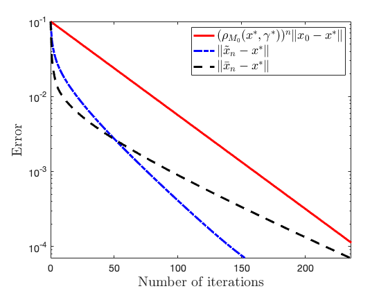
(a) $M_{0}=\|x_{0}-x^{*}\|=0.1$.

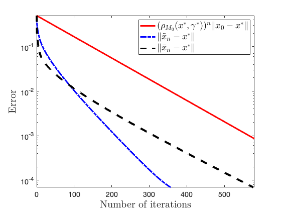
(b) $M_{0}=\|x_{0}-x^{*}\|=0.5$.

Figure 1: Numerical comparison of the theoretical upper bound and the errors of the algorithms in (DFB0) and (DFB1) for a tolerance of $7\cdot 10^{-5}$ and two initial conditions.

		DFB0				DFB1
$\|x_{0}-x^{*}\|$		$\gamma$	Time (s)	Iterations		$\gamma$	Time (s)	Iterations
$0.1$		$0.3748$	$170.343$	$153$		$0.3748$	$3.609$	$236$
$0.5$		$0.2132$	$566.695$	$357$		$0.2132$	$8.486$	$577$

Table 1: Performance of (DFB0) and (DFB1), for different initialization when the number of grid nodes (DoF) is $60^{2}$ and the tolerance is $7\cdot 10^{-5}$.

5.2 A second order mean field game with logarithmic and power couplings

Let $\nu\in\left]0,+\infty\right[$, $\alpha\in\left]1,2\right]$, and $\epsilon\in\left[0,+\infty\right[$. We consider the MFGs system

$$-\nu\Delta u+\frac{1}{2}\|\nabla u\|^{2}+\lambda =m^{\alpha-1}+\epsilon\log m+\widetilde{H}(x,y)\quad\text{in }\mathbb{T}^{2},$$

$$-\nu\Delta m-\text{div}\big{(}m\nabla u\big{)} =0\quad\text{in }\mathbb{T}^{2},$$

$$\int_{\mathbb{T}^{2}}u(x){\rm d}x=0, \>\>\int_{\mathbb{T}^{2}}m(x){\rm d}x=1,\>m>0,$$ (69)

where, for all $(x,y)\in\mathbb{T}^{2}$,

$$\widetilde{H}(x,y)=-\frac{\sin(2\pi x)+\sin(2\pi y)+\cos(4\pi x)}{2}.$$

We consider the finite difference approximation (45) of the system above, which corresponds to the optimality condition of Problem 6 with $\ell=|\cdot|^{2}/2+\iota_{\left[0,+\infty\right[}$ and

$$F_{i,j}\colon\rho\mapsto\begin{cases}\frac{1}{\alpha}\rho^{\alpha}+c_{i,j}\rho+\epsilon\,\rho(\log\rho-1),&\text{if}\>\>\rho>0;\\ 0,&\text{if}\>\>\rho=0;\\ {+\infty},&\text{if}\>\>\rho<0,\end{cases}$$ (70)

where, for every $i,j\in\{0,\ldots,N-1\}$, $c_{i,j}=\widetilde{H}(ih,jh)$.

	CP				DR				DFB0				DFB1
$\nu$	Time (s)	Iterations	$\gamma$		Time (s)	Iterations	$\gamma$		Time (s)	Iterations	$\gamma$		Time (s)	Iterations	$\gamma$
$0.1$	$5.285$	$26$	$1.05$		$5.2094$	$26$	$1.05$		$34.4958$	$23$	$0.6$		$1.6456$	$30$	$0.65$
$0.5$	$3.1873$	$16$	$1.05$		$3.1924$	$16$	$1.05$		$17.4105$	$12$	$0.55$		$0.50957$	$10$	$0.55$

Table 2: Performance comparison among CP, DR, (DFB0), and (DFB1), for varying values of $\nu$ when $\epsilon=0$ and the number of grid nodes (DoF) is $60^{2}$.

	CP				DR				DFB0				DFB1
$\nu$	Time (s)	Iterations	$\gamma$		Time (s)	Iterations	$\gamma$		Time (s)	Iterations	$\gamma$		Time (s)	Iterations	$\gamma$
$0.1$	$5.6857$	$26$	$0.95$		$5.5486$	$26$	$0.95$		$32.6036$	$22$	$0.7$		$1.4765$	$27$	$0.75$
$0.5$	$3.5337$	$17$	$0.95$		$3.5753$	$17$	$0.95$		$13.831$	$10$	$0.65$		$0.48746$	$10$	$0.65$

Table 3: Performance comparison among CP, DR, (DFB0), and (DFB1), for varying values of $\nu$ when $\epsilon=0.1$ and the number of grid nodes (DoF) is $60^{2}$.

	CP				DR				DFB0				DFB1
$\nu$	Time (s)	Iterations	$\gamma$		Time (s)	Iterations	$\gamma$		Time (s)	Iterations	$\gamma$		Time (s)	Iterations	$\gamma$
$0.1$	$7.9191$	$25$	$0.8$		$7.561$	$25$	$0.8$		$25.3507$	$17$	$1$		$1.3145$	$20$	$1.1$
$0.5$	$5.6428$	$20$	$0.75$		$5.4536$	$20$	$0.75$		$15.2802$	$8$	$1.05$		$0.49585$	$8$	$1.1$

Table 4: Performance comparison among CP, DR, (DFB0), and (DFB1), for varying values of $\nu$ when $\epsilon=0.5$ and the number of grid nodes (DoF) is $60^{2}$.

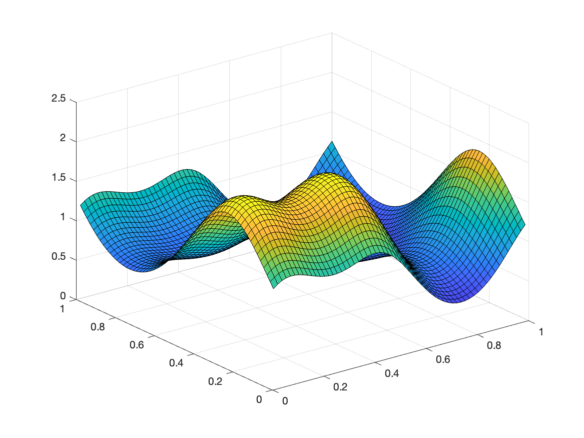
(a) $\epsilon=0,\>\>\nu=0.1$.

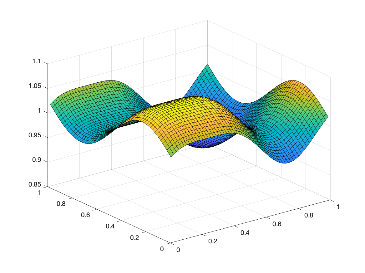
(b) $\epsilon=0,\>\>\nu=0.5$.

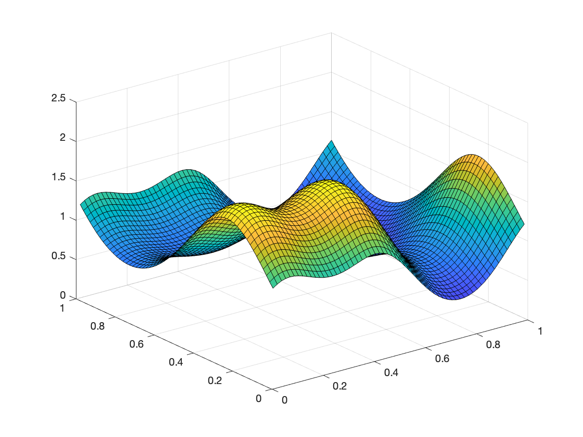
(c) $\epsilon=0.1,\>\>\nu=0.1$.

(d) $\epsilon=0.1,\>\>\nu=0.5$.

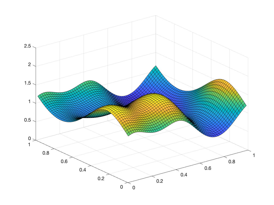
(e) $\epsilon=0.5,\>\>\nu=0.1$.

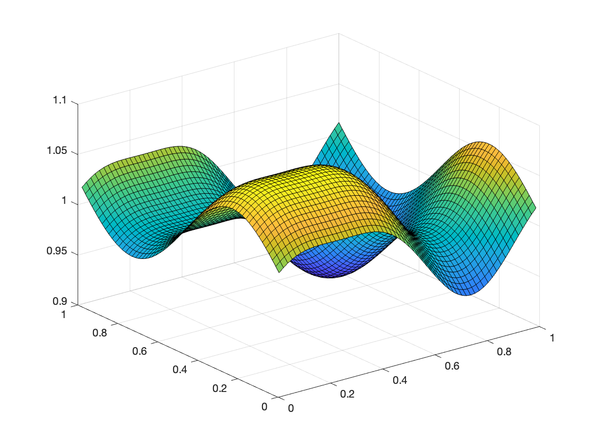
(f) $\epsilon=0.5,\>\>\nu=0.5$.

Figure 2: Numerical results of (DFB1) for different values of $\epsilon$ and $\nu$.

Since, for every $i,j\in\{0,\ldots,N-1\}$, $F_{i,j}$ and $\ell$ are supercoercive and strictly convex on their domains, Proposition 8(ii) implies that $\phi^{*}_{i,j}\colon(\theta_{i,j},v_{i,j})\mapsto F_{i,j}^{*}(\theta_{i,j}+\|v_{i,j}\|^{2}/2)$ is everywhere defined, differentiable, and

$$\nabla\phi_{i,j}^{*}\colon(\theta_{i,j},v_{i,j})\mapsto(F_{i,j}^{*})^{\prime}(\theta_{i,j}+\|v_{i,j}\|^{2}/2)\begin{pmatrix}1\\ v_{i,j}\end{pmatrix}.$$ (71)

In the case when $\epsilon>0$, we have, for every $i,j\in\{0,\ldots,N-1\}$, $\text{\rm dom}\,\partial F_{i,j}=\text{\rm ran}\,(F_{i,j}^{*})^{\prime}=\left]0,+\infty\right[$ and, therefore, for every $(\rho,y)\in\mathbb{R}\times\left]0,+\infty\right[$,

$$\quad\quad\,\,\ y=(F_{i,j}^{*})^{\prime}(\rho)$$

$$\Leftrightarrow\quad\rho=F_{i,j}^{\prime}(y)=y^{\alpha-1}+c_{i,j}+\epsilon\ln(y)$$

$$\Leftrightarrow\quad\Big{(}\frac{\alpha-1}{\epsilon}\Big{)}(\rho-c_{i,j})+\ln\Big{(}\frac{\alpha-1}{\epsilon}\Big{)}=\Big{(}\frac{\alpha-1}{\epsilon}\Big{)}y^{\alpha-1}+\ln\bigg{(}\Big{(}\frac{\alpha-1}{\epsilon}\Big{)}y^{\alpha-1}\bigg{)}$$

$$\Leftrightarrow\quad\Big{(}\frac{\alpha-1}{\epsilon}\Big{)}e^{\big{(}\frac{\alpha-1}{\epsilon}\big{)}(\rho-c_{i,j})}=\bigg{(}\Big{(}\frac{\alpha-1}{\epsilon}\Big{)}y^{\alpha-1}\bigg{)}e^{\big{(}\frac{\alpha-1}{\epsilon}\big{)}y^{\alpha-1}}$$

$$\Leftrightarrow\quad y=\Big{(}\frac{\epsilon}{\alpha-1}\Big{)}^{\frac{1}{\alpha-1}}W_{0}\bigg{(}\Big{(}\frac{\alpha-1}{\epsilon}\Big{)}e^{\big{(}\frac{\alpha-1}{\epsilon}\big{)}(\rho-c_{i,j})}\bigg{)}^{\frac{1}{\alpha-1}},$$ (72)

where $W_{0}$ stands for the principal branch of the Lambert W-function. On the other hand, in the case $\epsilon=0$, we have $\text{\rm dom}\,\partial F_{i,j}=\text{\rm ran}\,(F_{i,j}^{*})^{\prime}=\left[0,+\infty\right[$. Altogether, it follows from simple computations that

$$(F_{i,j}^{*})^{\prime}\colon\rho\mapsto\begin{cases}0,&\text{if}\>\>\epsilon=0\>\>\text{and}\>\>\rho<c_{i,j};\\ (\rho-c_{i,j})^{\frac{1}{\alpha-1}},&\text{if}\>\>\epsilon=0\>\>\text{and}\>\>\rho\geq c_{i,j};\\ \Big{(}\frac{\epsilon}{\alpha-1}\Big{)}^{\frac{1}{\alpha-1}}W_{0}\bigg{(}\Big{(}\frac{\alpha-1}{\epsilon}\Big{)}e^{\big{(}\frac{\alpha-1}{\epsilon}\big{)}(\rho-c_{i,j})}\bigg{)}^{\frac{1}{\alpha-1}},&\text{if}\>\>\epsilon>0.\end{cases}$$ (73)

Since $\alpha\in\left]1,2\right]$, for every $\epsilon\geq 0$ and $i,j\in\{0,\ldots,N-1\}$, the function $(F_{i,j}^{*})^{\prime}$ is Lipschitz continuous on bounded sets. Thus, we derive from (71) that Problem 6 is a particular instance of Problem 1.

As in Section 5.1, we denote by (DFB0) and (DFB1) the Algorithm 9 with $(C_{1},C_{2})=(K,\mathbb{R}^{4})$ and $(C_{1},C_{2})=(\mathbb{R}^{4},K)$, respectively. In Tables 2-4, we compare the computational time and number of iterations that algorithms (DFB0), (DFB1), Chambolle-Pock (CP) [26], and Douglas-Rachford (DR) [42] take to approximate a solution for the case when $\alpha=1.5$ with a tolerance of $\varepsilon=h^{3}$ for the relative error $\|(\theta_{n+1}-\theta_{n},v_{n+1}-v_{n})\|/\|(\theta_{n},v_{n})\|$. For CP, we use critical step-sizes, i.e., $\sigma\gamma=1$, where $\sigma>0$ and $\gamma>0$ are the step-sizes associated with dual and primal variable updates, respectively. This choice is justified by theoretical results ensuring convergence of CP with critical step-sizes [17, 20] and numerical results asserting that the numerical behavior of CP improves as $\sigma\gamma$ approaches $1$ [20]. Moreover, CP and DR show identical numerical behavior, which is justified by the fact that CP coincides with DR for critical step-sizes [26, 47]. We also observe that (DFB0) needs less number of iterations to achieve a relative error of $\varepsilon=h^{3}$, however its computational time is much larger because of the subiterations needed to compute the projection onto $D_{K}$. By considering computational time, (DFB1) is the more efficient algorithm, obtaining a time reduction up to 90% with respect to CP and DR. Moreover, note that the computational time of CP and DR increases as long as the parameter $\epsilon$ multiplying the entropy penalization increases. On the other hand, (DFB1) has similar computational time and even a smaller number of iterations to achieve the tolerance as $\epsilon$ increases. We display in Figure 2 the approximation of the equilibrium configurations $m^{h}$ that we obtain for different values of $\epsilon$ and the viscosity parameter $\nu$. Comparing the distributions on the left of Figure 2 with those on the right, we observe that, as expected, for larger viscosity parameters the diffusive behavior of equilibria prevails with regard to the individual preferences of the agents.

Acknowledgments

The work of Luis M. Briceño-Arias was supported by Agencia Nacional de Investigación y Desarrollo (ANID-Chile) under grants FONDECYT 1190871, FONDECYT 1230257, and by Centro de Modelamiento Matemático (CMM), ACE210010 and FB210005, BASAL funds for centers of excellence. The work of F. J. Silva was partially supported by l’Agence Nationale de la Recherche (ANR), project ANR-22-CE40-0010, and by KAUST through the subaward agreement ORA-2021-CRG10-4674.6. X. Yang was partly funded by the Air Force Office Scientific Research under MURI award number FA9550-20-1-0358 (Machine Learning and Physics-Based Modeling and Simulation).