Positive Label Is All You Need for Multi-Label Classification

Abstract

Multi-label classification (MLC) suffers from the inevitable label noise in training data due to the difficulty in annotating various semantic labels in each image. To mitigate the influence of noisy labels, existing methods mainly devote to identifying and correcting the label mistakes via a trained MLC model. However, these methods still involve annoying noisy labels in training, which can result in imprecise recognition of noisy labels and weaken the performance. In this paper, considering that the negative labels are substantially more than positive labels, and most noisy labels are from the negative labels, we directly discard all the negative labels in the dataset, and propose a new method dubbed positive and unlabeled multi-label classification (PU-MLC). By extending positive-unlabeled learning into MLC task, our method trains model with only positive labels and unlabeled data, and introduces adaptive re-balance factor and adaptive temperature coefficient in the loss function to alleviate the catastrophic imbalance in label distribution and over-smoothing of probabilities in training. Furthermore, to capture both local and global dependencies in the image, we also introduce a local-global convolution module, which supplements global information into existing convolution layers with no retraining of backbone required. Our PU-MLC is simple and effective, and it is applicable to both MLC and MLC with partial labels (MLC-PL) tasks. Extensive experiments on MS-COCO and PASCAL VOC datasets demonstrate that our PU-MLC achieves significantly improvements on both MLC and MLC-PL settings with even fewer annotations. Code will be released.

Introduction

Deep learning has achieved remarkable success in single-label image classification task (He et al. 2016; Simonyan and Zisserman 2014; Szegedy et al. 2016). Recently, multi-label classification (MLC) (Chen et al. 2019c, b; Ridnik et al. 2021a) has attracted much attention as an image often contains multiple objects or concepts. Existing methods usually treat MLC as multiple binary classification tasks and train each binary task with positive and negative labels. As such, the model is trained to recognize whether an image contains each class or not.

However, noisy labels inevitably exist in MLC datasets due to the annotation difficulty (Durand, Mehrasa, and Mori 2019; Ridnik et al. 2021a), which disturb the training and worsen the performance as a result (see Figure 2(a)-(b)). To alleviate this issue, some methods (Thyagarajan et al. 2022; Ridnik et al. 2021a) propose to first train the model with noisy labels, then correct or discard the mislabeled labels with the learned model. Nevertheless, the mislabeled labels are still involved in these methods, which would still cause a negative impact on training process and mislead the identification of noisy labels to some extent.

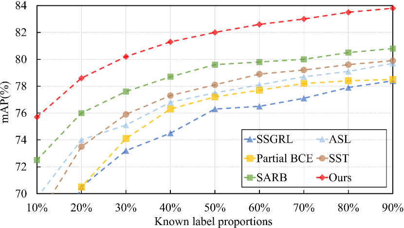
Figure 1: Comparison of multi-label classification performance on MS-COCO. Our PU-MLC gains significant improvements on all known label proportions.

Moreover, the mislabeling problem tends to be severer on multi-label classification with partial labels (MLC-PL) task (Durand, Mehrasa, and Mori 2019; Huynh and Elhamifar 2020; Chen et al. 2022b; Pu et al. 2022). In MLC-PL, models are trained with a partially labeled dataset to reduce the annotation cost (see Figure 2(c)), and the model would be more sensitive to the noise on such a small proportion of labels. To solve the above problem, some works (Durand, Mehrasa, and Mori 2019; Huynh and Elhamifar 2020) attempt to re-weight the loss of each sample to weaken the influence of noisy labels; some other works use semantic-aware representations to generate pseudo labels (Chen et al. 2022b) or blend category-specific semantic representation between different images (Pu et al. 2022). However, similar to the aforementioned methods in MLC, these MLC-PL methods still use mislabeled samples in training, which would lead to imprecise evaluation on loss weights and pseudo labels, and thus degrade the performance.

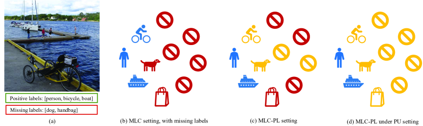
Figure 2: Comparisons of different learning methods in MLC. (a) an image from MS-COCO train2014 which has two missing labels. To train the sample image, (b) missing labels in traditional MLC methods are mistakenly classified as negative labels; (c) MLC-PL samples a proportion of labels, but still encounters false negative labels; (d) Our method treats all negative labels as unlabeled ones. Blue, red, and yellow icons denote positive, negative, and unknown labels, respectively.

Considering the above discussions, as involving the noisy labels in training would lead to inferior performance on MLC and MLC-PL, can we just remove them before training? Frustratingly, we do not have an oracle that can precisely identify noisy labels. In this paper, we propose a more radical way, that is, if we cannot identify noisy labels, we just remove all the labels. Inspired by positive-unlabeled (PU) learning (Plessis, Niu, and Sugiyama 2015; Kiryo et al. 2017; Chen et al. 2020), which trains binary classifiers using labels on one (positive) category only and achieves competitive performance to traditional positive-negative (PN) learning (see Figure 2(d)), we propose to discard all the negative labels and train MLC models with only positive and unlabeled data. Since the negative labels are considerably more than positive labels in MLC datasets (see Figure 3), removing negative labels can avoid most of the annotation errors in training. Furthermore, PU learning is acknowledged to be more robust and accurate than PN learning when the negative labels are noisy, since the PN may learn to rely on noisy negative labels and make incorrect predictions. In contrast, PU adopts unbiased risk estimator to perform a proper approximation to PN without noisy labels, and the soft labels in estimator is more informative and accurate to label the sample compared to the hard label in previous methods.

As a result, we propose a method based on PU learning, dubbed as positive and unlabeled multi-label classification (PU-MLC). Concretely, we extend the conventional PU learning to the task of combining multiple binary classifications in MLC. Besides, to deal with the catastrophic imbalance between positive and negative labels in MLC task, we propose an adaptive re-balance factor in PU loss to balance the loss weight. Since it could be much more challenging to train multiple binary classification tasks in MLC than the simple practice in current PU learning methods, we further propose an adaptive temperature coefficient module to adjust the sharpness of predicted probabilities in loss, which effectively avoids the probabilistic distribution to be over-smooth in the early stage of training, and thus benefits the optimization. Moreover, to effectively incorporate both local and global dependencies within the image, we introduce a novel local-global convolution module. This module seamlessly integrates global information into existing convolution layers without necessitating a retraining of the backbone.

Our proposed PU-MLC is simple and effective, and applies to both MLC and PU-MLC tasks. Meanwhile, it can obtain promising performance with only a small portion of positive labels, which could also reduce the cost of annotating. Extensive experiments on two benchmark datasets MS-COCO (Lin et al. 2014) and PASCAL VOC 2007 (Everingham et al. 2010) demonstrate that our PU-MLC achieves significantly improvements on both MLC and MLC-PL settings, with even fewer annotated labels used. For example, on MLC-PL, our PU-MLC improves the state-of-the-art SARB (Pu et al. 2022) by 3.2% mAP under 10% known label ratio on MS-COCO (see Figure 1); while on MLC, our PU-MLC achieves an extraordinary 84.2% mAP on MS-COCO, surpassing our PN learning baseline by 6.9%.

Related Work

Multi-Label Classification

Multi-label classification (MLC) task aims to recognize semantic categories in a given image, which usually contains multiple objects or concepts. Previous works (Chen et al. 2019a, c; You et al. 2020) propose to construct pairwise statistical correlations using the first-order adjacency matrix obtained by graph convolutional networks (GCN) (Kipf and Welling 2016). Although the above methods achieve noteworthy success, they cannot extract higher-order correlations and can attract overfitting on small training sets. Some works (Lanchantin et al. 2021; Zhao et al. 2021) introduce transformer to extract complicated dependencies among visual features and labels.

MLC with partial labels (MLC-PL). Traditional multi-label classification (MLC) tasks rely on fully annotated datasets, and making such datasets is expensive, time-consuming, and error-prone. To reduce the cost of annotation, multi-label classification with partial labels (MLC-PL) attempts to train models with partially-annotated labels per image, which both contain positive and negative labels. Recent works (Durand, Mehrasa, and Mori 2019; Huynh and Elhamifar 2020; Chen et al. 2022b) propose to generate pseudo labels to those unknown samples based on the learned knowledge in the training model, and then train the model with ground-truth partial labels and generated pseudo labels.

Positive-Unlabeled (PU) learning

Different from the traditional positive-negative (PN) learning in the binary classification task, PU learning aims to train the model with only positive and unknown labels (Bekker and Davis 2020). Recent advances (Plessis, Niu, and Sugiyama 2015; Kiryo et al. 2017; Chen et al. 2020; Huang et al. 2022b) have achieved remarkable progress in deep learning. However, these methods rely heavily on the class prior estimation. While the class prior in the training dataset may not always correctly represent the label distribution in the validation set, and thus performing PU learning without class prior becomes an emergent topic (Chen et al. 2020; Hu et al. 2021; Chang, Du, and Zhang 2021; Gong et al. 2021). For example, vPU (Chen et al. 2020) proposes a variational principle to achieve superior performance without class prior. In this paper, we extend PU learning to MLC task based on vPU (Chen et al. 2020).

Proposed Approach: PU-MLC

In this section, we propose our method PU-MLC for multi-label classification (MLC) in deep learning. We extend the positive-unlabeled (PU) learning method vPU (Chen et al. 2020) to handle MLC tasks with multiple binary classification sub-tasks. We address the issue of imbalanced label distributions in MLC datasets by introducing a re-balance factor in the PU loss. This factor dynamically adjusts the loss weight based on predicted probabilities, improving performance. To handle the optimization of multiple PU learning tasks in PU-MLC, we propose an adaptive temperature coefficient module. This module prevents over-smoothing of the probabilistic distribution during early training stages. Additionally, we introduce a local-global convolution module to capture both local and global dependencies within images. This module seamlessly integrates global information into existing convolution layers without requiring retraining of the backbone network.

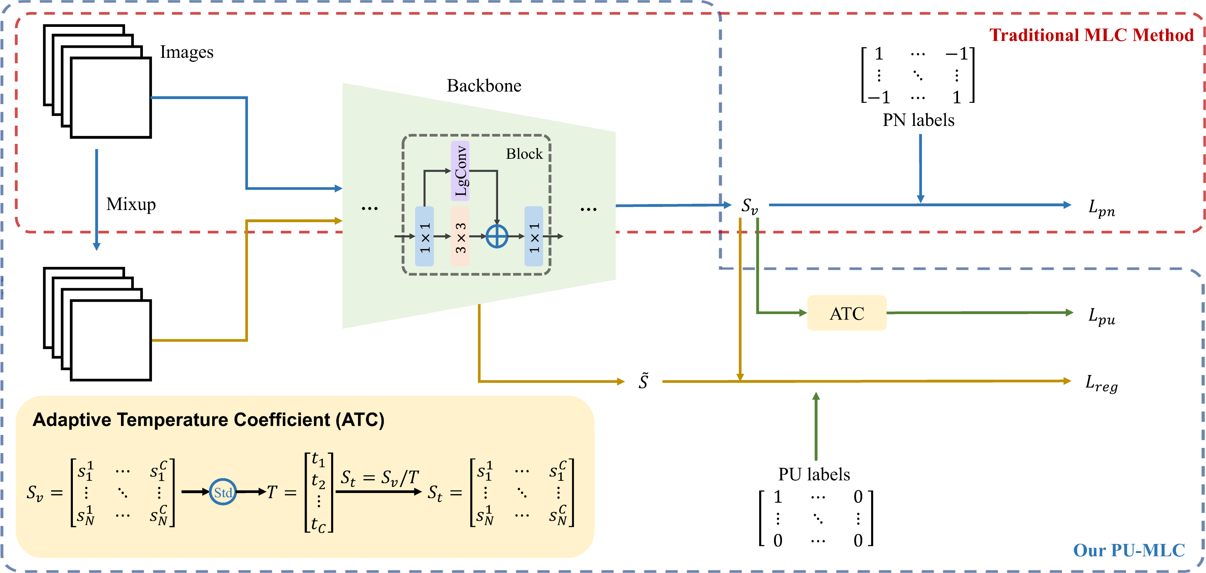
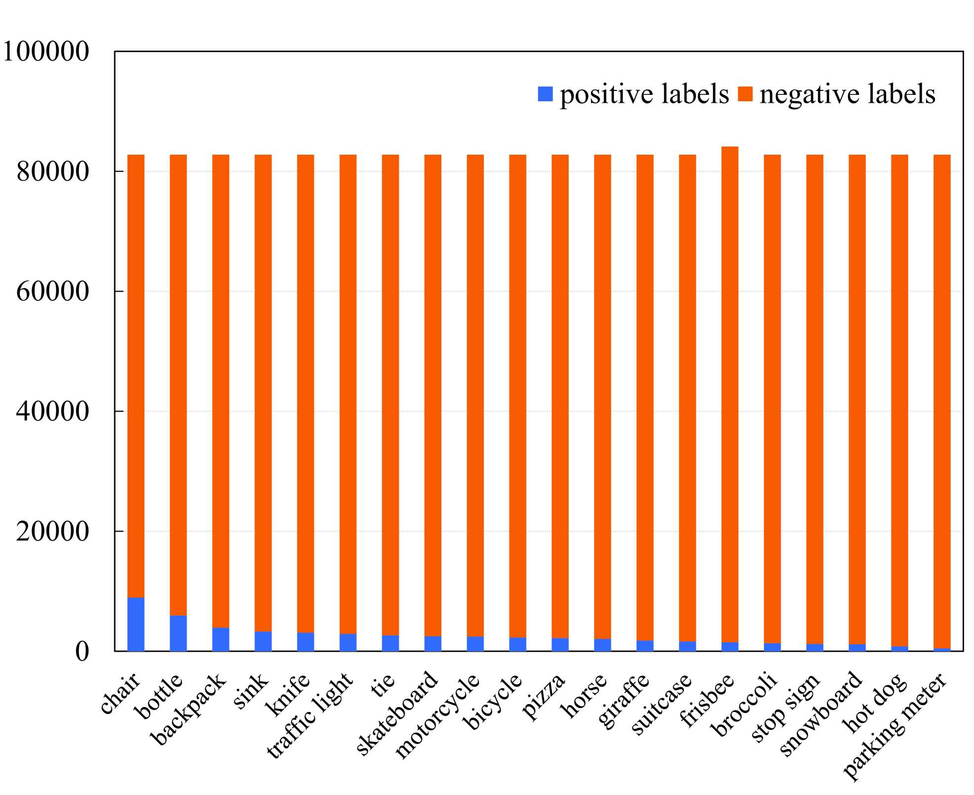
Figure 3: (a) Overview of our proposed PU-MLC. Instead of using positive and negative labels in the traditional MLC method (red box), our PU-MLC conducts a positive-unlabeled (PU) learning strategy with only partial positive labels leveraged. Besides, we introduce mixup regularization loss and the adaptive temperature coefficient module to further boost the performance. Additionally, we enhance the global representations in backbone by integrating a local-global convolution module to every $3\times 3$ local convolutions. Std: standard deviation. (b) Histograms of the number of positive and negative labels in each category. We randomly select 20 categories from MS-COCO train set.

MLC as PU learning

MLC as PN learning. MLC task is usually formulated as multiple binary classification sub-tasks, and each sub-task aims to recognize whether a specific category is in the input image. Formally, for a MLC task with $C$ categories, let $\bm{s}\in\mathbb{R}^{N\times C}$ and $\bm{y}\in\{-1,+1\}^{N\times C}$ be the predicted logits and the ground-truth positive and negative (PN) labels, respectively, where $N$ denotes batch size, the overall classification loss is formulated as

$$\mathcal{L}_{\mathrm{mlc}}= \frac{1}{C\times N}\sum_{c=1}^{C}\sum_{n=1}^{N}[\mathds{1}(y_{n,c}=+1)\mathcal{L}_{+}(\sigma(s_{n,c}))$$ (1)

$$+\mathds{1}(y_{n,c}=-1)\mathcal{L}_{-}(\sigma(s_{n,c}))],$$

where $\sigma(\cdot)$ is the Sigmoid function, $\mathds{1}(\cdot)$ is an indicator function that takes the value 1 only if the condition is true and 0 otherwise, $\mathcal{L}_{+}$ and $\mathcal{L}_{-}$ denote losses on positive and negative labels, respectively.

Before presenting our PU-learning based MLC method, we first rewrite the learning objective of the above positive-negative (PN) classification loss ((1)) as the expected risk on the training set. The total risk $R_{\mathrm{mlc}}$ is accumulated with all PN sub-tasks, and for each task (category) with the class prior (proportion of positive labels) $\pi_{\mathrm{p}}$ and $\bm{S}\in\mathbb{R}^{M}$ being its corresponding logits on the training set with $M$ images, its risk is formulated as

$$R_{\mathrm{pn}} =\pi_{\mathrm{p}}\mathbb{E}_{\mathcal{P}}[\mathcal{L}_{+}(\sigma(\bm{S}))]+(1-\pi_{\mathrm{p}})\mathbb{E}_{\mathcal{N}}[\mathcal{L}_{-}(\sigma(\bm{S}))],$$ (2)

where the images regarding to their label types are split into positive set $\mathcal{P}$ and negative set $\mathcal{N}$, and we have the expectations of positive and negative losses

$$\mathbb{E}_{\mathcal{P}}[\mathcal{L}_{+}(\sigma(\bm{S}))]=\frac{1}{|\mathcal{P}|}\sum_{s_{m}\in\mathcal{P}}\mathcal{L}_{+}(\sigma(s_{m})),$$ (3)

$$\mathbb{E}_{\mathcal{N}}[\mathcal{L}_{-}(\sigma(\bm{S}))]=\frac{1}{|\mathcal{N}|}\sum_{s_{m}\in\mathcal{N}}\mathcal{L}_{-}(\sigma(s_{m})).$$

PN to PU. In this paper, we aim to train a MLC model with only positive labels; i.e., our training set is composed of a positive set $\mathcal{P}$ and an unlabeled set $\mathcal{U}$ (mixture of unlabeled positive and negative images). Nevertheless, the negative labels are unavailable in our PU setting, and therefore we cannot directly optimize (2) to obtain our model. In order to train a classifier with positive and unknown labels, a classical method uPU (Plessis, Niu, and Sugiyama 2015) introduces an unbiased formulation to the PN learning by rewriting the expectation of negative classification loss $\mathbb{E}_{\mathcal{N}}[\mathcal{L}_{-}(\sigma(\bm{S}))]$ to

$$(1-\bm{\pi}_{\mathrm{p}})\mathbb{E}_{\mathcal{N}}[\mathcal{L}_{-}(\sigma(\bm{S}))] =\mathbb{E}_{\mathcal{U}}[\mathcal{L}_{-}(\sigma(\bm{S}))]$$ (4)

$$-\bm{\pi}_{\mathrm{p}}\mathbb{E}_{\mathcal{P}}[\mathcal{L}_{-}(\sigma(\bm{S}))],$$

and thus (2) could be converted to PU format:

$$R_{\mathrm{pu}} =\bm{\pi}_{\mathrm{p}}\mathbb{E}_{\mathcal{P}}[\mathcal{L}_{+}(\sigma(\bm{S}))]$$ (5)

$$-\bm{\pi}_{\mathrm{p}}\mathbb{E}_{\mathcal{P}}[\mathcal{L}_{-}(\sigma(\bm{S}))]+\mathbb{E}_{\mathcal{U}}[\mathcal{L}_{-}(\sigma(\bm{S}))],$$

However, the above method easily causes overfitting in deep neural networks and rely heavily on the class prior, and we empirically find that it performs poorly on the multi-label classification task, as the task is more challenging and many categories have very small class priors. Fortunately, there are some recent studies (Hu et al. 2021; Chang, Du, and Zhang 2021; Gong et al. 2021) propose to mitigate these issues, and our PU-MLC is developed based on vPU (Chen et al. 2020), which proposes a novel loss function based on the variational principle to approximate the ideal classifier without the class prior:

$$R_{\mathrm{var}}=\log{\mathbb{E}_{\mathcal{U}}[\sigma(\bm{S})]}-\mathbb{E}_{\mathcal{P}}[\log{\sigma(\bm{S})}].$$ (6)

Therefore, for each category $c$, the classification loss becomes

$$\mathcal{L}_{\mathrm{var}}^{(c)}= \log(\frac{1}{|\mathcal{U}^{(c)}_{N}|}\sum_{s_{u}\in\mathcal{U}^{(c)}_{N}}\sigma(s_{u}))$$ (7)

$$-\frac{1}{|\mathcal{P}^{(c)}_{N}|}\sum_{s_{p}\in\mathcal{P}^{(c)}_{N}}\log\sigma(s_{p}),$$

here $\mathcal{P}^{(c)}_{N}$ and $\mathcal{U}^{(c)}_{N}$ denote positive samples and unlabeled samples of category $c$ in each mini-batch, respectively.

Besides, vPU also introduces a consistency regularization term based on Mixup (Zhang et al. 2017), which alleviates the overfitting problem and increases the robustness in PU learning, i.e.,

$$\mathcal{L}_{\mathrm{reg}}^{(c)}=\frac{2}{N}\sum^{N/2}_{n=1}(\log(\sigma(\hat{s}_{n,c}))-\log(\sigma(\tilde{s}_{n,c})))^{2},$$ (8)

with

$$\mu\overset{iid}{\sim}\mathrm{Beta}(\delta,\delta),$$ (9)

$$\hat{\bm{s}}=\mu\cdot\bm{s}^{\prime}+(1-\mu)\cdot\bm{s}^{\prime\prime},$$

$$\tilde{\bm{s}}=\Phi(\mu\cdot\bm{x}^{\prime}+(1-\mu)\cdot\bm{x}^{\prime\prime}),$$

where $\bm{s}^{\prime}$ and $\bm{s}^{\prime\prime}$ are the first and last halves of predicted logits $\bm{s}\in\mathbb{R}^{N\times C}$, $\bm{x}^{\prime}$ and $\bm{x}^{\prime\prime}$ represent the first and last halves of input images $\bm{x}$, and $\tilde{\bm{s}}$ denotes the prediction of the model $\Phi$ with mixed images as input.

As a result, in our PU-MLC, the traditional MLC loss in (1) is replaced with our PU loss, and the overall loss function is formulated as

$$\mathcal{L}_{\mathrm{pu-mlc}}=\sum_{c=1}^{C}(\mathcal{L}_{\mathrm{var}}^{(c)}+\lambda\mathcal{L}_{\mathrm{reg}}^{(c)}),$$ (10)

where $\lambda$ is a scalar to balance the losses and we set $\lambda=1$ in all experiments.

Note that unlike conventional PU learning, we complement all the positive samples in $\mathcal{P}$ into $\mathcal{U}$ to keep the unlabeled set $\mathcal{U}$ have a similar label distribution as the traditional training set, which is important for PU learning (see ablation studies in Section Ablation Studies for details).

Catastrophic Imbalance of Label Distribution

In MLC datasets, the total number of negative labels are generally much larger than the positive labels, as summarized in Figure 3. Since our PU-MLC removes all the negative labels and appends them into the unlabeled set, the number of samples contributing to the first and second terms of $\mathcal{L}_{\mathrm{var}}$ in (7) are extremely discrepant in each mini-batch. However, in PU learning methods, the positive and negative samples are carefully designed to have the same size in one batch, and directly optimize (7) in our method would make the unlabeled term dominate the optimization result in poor result in MLC-PL when the known label ratio is low (e.g., only 51.8% mAP with 10% positive labels).

To alleviate the catastrophic imbalance of label distribution, we aim to narrow down the loss weight of unlabeled term to decrease its importance in optimization. Inspired by focal loss (Lin et al. 2017) and ASL (Ridnik et al. 2021a), we propose a re-balance factor to dynamically re-weight the unlabeled loss based on the predicted probabilities on unlabeled samples, and (7) is reformulated as

$$\mathcal{L}_{\mathrm{var}}^{(c)}= p^{\gamma}_{c}\log(\frac{1}{|\mathcal{U}^{(c)}_{N}|}\sum_{s_{u}\in\mathcal{U}^{(c)}_{N}}\sigma(s_{u}))$$ (11)

$$-\frac{1}{|\mathcal{P}^{(c)}_{N}|}\sum_{s_{p}\in\mathcal{P}^{(c)}_{N}}\log\sigma(s_{p}),$$

where $p_{c}^{\gamma}$ denotes our re-balance factor, with $p_{c}=\frac{1}{|\mathcal{U}|}\sum_{s_{u}\in\mathcal{U}}\sigma(s_{u})$ being the mean probability of unlabeled samples, and $\gamma$ is used to control the value of the factor. In our experiments, we set larger $\gamma$ for smaller known label ratios, as the imbalance is severer on smaller ratios and we need a smaller weight on unlabeled loss to balance the loss.

Table 1: The comparisons on MS-COCO and VOC 2007 under different known label ratios. Note that our PU-MLC only uses partial positive labels, while other methods train models with the same number of positive labels and additional negative labels. ^∗ indicates the backbone is pretrained by CLIP (Radford et al. 2021). Results except DualCoOp and our method are reported by SARB (Pu et al. 2022).

Datasets	Methods	10%	20%	30%	40%	50%	60%	70%	80%	90%	Avg. mAP	Avg. OF1	Avg. CF1
MS-COCO	SSGRL	62.5	70.5	73.2	74.5	76.3	76.5	77.1	77.9	78.4	74.1	73.9	68.1
	ML-GCN	63.8	70.9	72.8	74.0	76.7	77.1	77.3	78.3	78.6	74.4	73.1	68.4
	KGGR	66.6	71.4	73.8	76.7	77.5	77.9	78.4	78.7	79.1	75.6	73.7	69.7
	P-GCN	67.5	71.6	73.8	75.5	77.4	78.4	79.5	80.7	81.5	76.2	-	-
	ASL	69.7	74.0	75.1	76.8	77.5	78.1	78.7	79.1	79.7	76.5	46.7	47.9
	CL	26.7	31.8	51.5	65.4	70.0	71.9	74.0	77.4	78.0	60.7	61.9	48.3
	Partial BCE	61.6	70.5	74.1	76.3	77.2	77.7	78.2	78.4	78.5	74.7	74.0	68.8
	SST	68.1	73.5	75.9	77.3	78.1	78.9	79.2	79.6	79.9	76.7	-	-
	SARB	72.5	76.0	77.6	78.7	79.6	79.8	80.0	80.5	80.8	78.4	76.8	72.7
	PU-MLC	75.7	78.6	80.2	81.3	82.0	82.6	83.0	83.5	83.8	81.2	77.4	75.7
	DualCoOp∗	78.7	80.9	81.7	82.0	82.5	82.7	82.8	83.0	83.1	81.9	78.1	75.3
	PU-MLC∗	80.2	83.2	84.4	85.6	85.9	86.6	87.0	87.1	87.5	85.3	81.7	79.1
VOC 2007	SSGRL	77.7	87.6	89.9	90.7	91.4	91.8	92.0	92.2	92.2	89.5	87.7	84.5
	ML-GCN	74.5	87.4	89.7	90.7	91.0	91.3	91.5	91.8	92.0	88.9	87.3	84.6
	KGGR	81.3	88.1	89.9	90.4	91.2	91.3	91.5	91.6	91.8	89.7	86.5	84.7
	P-GCN	82.5	85.4	88.2	89.8	90.0	90.9	91.6	92.5	93.1	89.3	-	-
	ASL	82.9	88.6	90.0	91.2	91.7	92.2	92.4	92.5	92.6	90.5	41.0	40.9
	CL	44.7	76.8	88.6	90.2	90.7	91.1	91.6	91.7	91.9	84.1	83.8	75.4
	Partial BCE	80.7	88.4	89.9	90.7	91.2	91.8	92.3	92.4	92.5	90.0	87.9	84.8
	SST	81.5	89.0	90.3	91.0	91.6	92.0	92.5	92.6	92.7	90.4	-	-
	SARB	85.7	89.8	91.8	92.0	92.3	92.7	92.9	93.1	93.2	91.5	88.3	86.0
	PU-MLC	88.0	90.7	91.9	92.0	92.4	92.7	93.0	93.4	93.5	92.0	88.2	86.5
	DualCoOp∗	90.3	92.2	92.8	93.3	93.6	93.9	94.0	94.1	94.2	93.2	86.3	84.2
	PU-MLC∗	91.3	92.9	93.3	93.7	93.8	94.3	94.5	94.6	94.8	93.7	89.8	88.2

Adaptive Temperature Coefficient

In PU learning, the training model actually acts as an estimator to generate the probabilistic estimation on each unlabeled samples and optimize them with the unlabeled loss term (Bekker and Davis 2020). However, the task of learning multiple binary classifiers in MLC is much more challenging than learning a single binary classifier in conventional PU learning methods. This gap in learning difficulty leads to a smaller convergent rate at the earlier phase of training, and thus the predicted probabilistic distribution is over-smooth, which makes the unlabeled loss less effective.

To adjust the smoothness of probabilistic distribution, we follow (Hinton, Vinyals, and Dean 2015) and propose a temperature coefficient $\tau$ to scale the logit values, i.e.,

$$\bm{s}_{t}=\bm{s}/\tau,$$ (12)

then the $\bm{s}_{t}$ is fed into the PU loss in place of the original $\bm{s}$.

By setting $\tau<1$, we can make the probabilistic distribution sharper, and thus provide more informative and effective signals to the loss. However, we empirically find that fixed temperature coefficient can only improve the performance on specific known label ratios and dataset (see Table 5). For example, MS-COCO dataset wants a $\tau<1$ to gain improvements, while $\tau<1$ performs worse than $\tau>1$ on VOC. This implies that, for different datasets with different learning difficulties, even for different categories in the same dataset, the optimal $\tau$ are different and needs to be set individually.

As a result, we propose an adaptive temperature coefficient module to first measure the sharpness of each category in each batch, then apply independent temperatures on each category. Formally, given the predicted logits $\bm{s}$, the sharpness of each category $c$ is measured using the standard deviation of the logits, and then the temperature is obtained by multiplying a scalar $\alpha$ onto the sharpness value, i.e.,

$$\tau^{(c)}=\min(\alpha\cdot\mathrm{Std}(\bm{s}_{c}),1).$$ (13)

We use a minimum function to ensure that the $\tau^{(c)}$ is less than or equal to 1, since we do not want the $\tau^{(c)}$ to exceed 1, which could even exacerbate the over-smooth.

The final PU loss $\mathcal{L}_{\mathrm{val}}^{(c)}$ becomes

$$\mathcal{L}_{\mathrm{var}}^{(c)}= p^{\gamma}_{c}\log(\frac{1}{|\mathcal{U}^{(c)}_{N}|}\sum_{s_{u}\in\mathcal{U}^{(c)}_{N}}\sigma(s_{u}/\tau^{(c)}))$$ (14)

$$-\frac{1}{|\mathcal{P}^{(c)}_{N}|}\sum_{s_{p}\in\mathcal{P}^{(c)}_{N}}\log\sigma(s_{p}/\tau^{(c)}).$$

Our adaptive temperature coefficient is suitable for different known label ratios and datasets, which could gain consistent improvements. The overall framework of our model is illustrated in Figure 3.

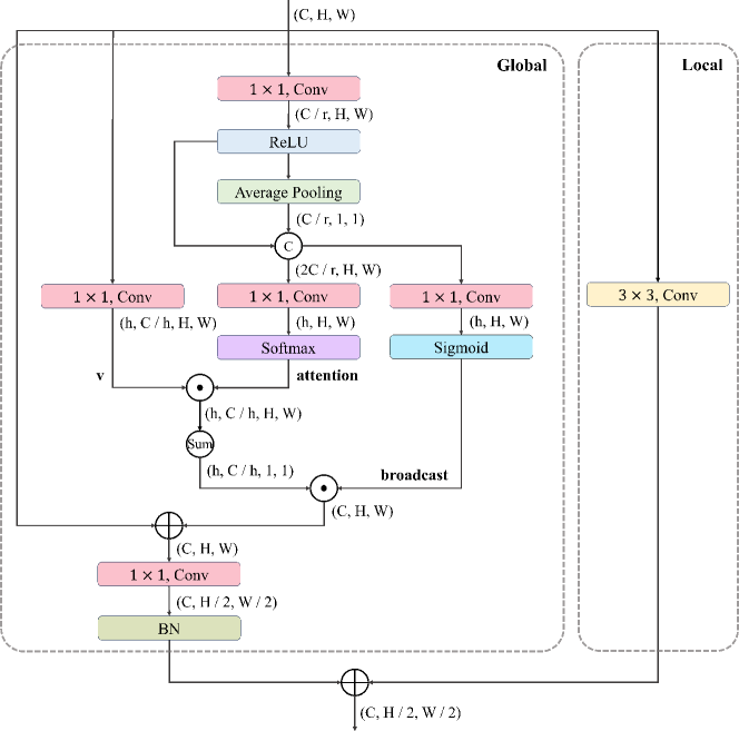
Figure 4: Illustration of Local-global convolution.

Local-Global Convolution

Recently, vision transformers (Dosovitskiy et al. 2020; Liu et al. 2021) have achieved significant improvements over the classical convolutional neural networks (CNNs) due to its capability of capturing global dependencies. However, transformers also suffers from large peak memory footprint, difficult deployment, and less effectiveness in light-weight models. As a results, in this paper, we aim to improve the CNNs with an alternative convolution-based global module named LgConv, which is plug-and-play and does not require additional re-pretraining of the backbone.

As shown in Figure 4, as a supplement of the original local convolution, the global branch in our LgConv first transform the input feature into hidden features that contains local information and global information (average pooling), then two $1\times 1$ convolutions are leveraged to generate multi-head attentions on spatial dimension and a broadcast attention that determines whether a global head should broadcast its information to each pixel, followed by Softmax and Sigmoid functions, respectively. As last, an $1\times 1$ convolution and a batch normalization are adopted to project the feature.

Since our global branch is initialized randomly in the pretrained backbone, directly supplementing its feature to the original feature would disturb the pretrained semantic information. Therefore, we propose to initialize the scale parameters $\bm{\gamma}$ in the last batch normalization layer with a small value ($0.0001$), and thus the global branch will have minor impacts to the original features at the beginning of training, and the backbone can be smoothly evolved.

Experiments

Datasets. To verify the efficacy of PU-MLC, we conduct extensive experiments on two popular benchmarks MS-COCO (Lin et al. 2014) and PASCAL VOC (Everingham et al. 2010).

Training strategies. Similar to previous works (Chen et al. 2022b; Pu et al. 2022), we adopt the ResNet-101 (He et al. 2016) as the backbone to extract image features, and then obtain logit scores with the same decoupling module and linear classifier. We initialize the backbone with parameters pre-trained on the ImageNet (Deng et al. 2009) dataset, and fix its parameters of the previous 91 layers except LgConv layers. We train the model for 40 epochs using Adam (Kingma and Ba 2014) optimizer and 1-cycle (Smith 2018) policy, with a maximum learning rate of 1e-4. During training, we resize the input image to 512 $\times$ 512, and adopt a random cropping with 512, 448, 384, 320, 256 resolutions, then the image is resized to 448 $\times$ 448, followed by a random horizontal flipping. During testing, we simply resize the input image to 448 $\times$ 448.

Results on MS-COCO

MLC-PL setting. To demonstrate the effectiveness of the PU-MLC, we compare our PU-MLC with current published state-of-the-art methods, including SSGRL (Chen et al. 2019a), ML-GCN (Chen et al. 2019c), KGGR (Chen et al. 2022a), P-GCN (Chen et al. 2021), ASL (Ridnik et al. 2021a), CL (Huynh and Elhamifar 2020), Partial BCE (Huynh and Elhamifar 2020), SST (Chen et al. 2022b), SARB (Pu et al. 2022) and DualCoOp (Sun, Hu, and Saenko 2022). As the experimental results shown in Table 1, our PU-MLC significantly outperforms previous methods under different known label ratios. For example, we surpass the results of P-GCN with 40% known labels with only 10% of positive labels. Besides, with 20% positive labels, our PU-MLC even obtains similar performance as 90% known labels in SSGRL. Moreover, on a high known label ratio of 90%, we obviously surpass SARB by 3.0% in mAP. Compared with previous methods, our method achieves state-of-the-art results in average mAP, OF1 and CF1, which are 81.2%, 77.4% and 75.7%, respectively. DualCoOp uses CLIP (Radford et al. 2021), a large-scale vision-language pre-trained model, as its backbone to achieve exceptional performance. For a fair comparison, by only using the same visual model, our method achieves superior performance than DualCoOp, which utilizes both visual and language models.

Note that these significant improvements are obtained with even fewer annotated labels used in training compared to other methods (e.g., with 10% known label ratio, we only use 10% positive labels, while other methods use 10% positive labels and 10% negative labels), this indicates that our method is more effective and efficient on limited training annotations. As shown in Table 2, the number of annotated labels used by PU-MLC in model training is much smaller than other methods based on PN. Concretely, our method achieves the best results while decreasing the amount of annotated labels by 96.4% at each known label ratio.

Table 2: Comparisons of the number of annotated labels used in training on MS-COCO. Reduction: the reduction ratio on used training annotations of our method compared to other methods.

Methods	PU-MLC			Others
	10%	50%	100%	10%	50%	100%
Positive	24,103	120,517	241,035	24,103	120,517	241,035
Negative	0	0	0	638,160	3,190,802	6,381,605
Total	24,103	120,517	241,035	662,263	3,311,319	6,622,640
Reduction	-96.4%	-96.6%	-96.4%	-	-	-

MLC setting. Since our method is designed for both MLC and MLC-PL tasks, we also conduct experiments to validate our performance on traditional MLC. As shown in Table 3, we achieve promising performance compared to previous methods. Similar to MLC-PL, our method in MLC is trained with only positive labels, and discards a large number of negative labels (negative labels are $\sim 26.5\times$ more than positive labels), our results can still outperform those methods trained with full annotations. Besides, compared with our PN learning baseline ResNet-101 (He et al. 2016), our MLC-PL significantly outperforms it by 6.9% in mAP, which demonstrates that our method is beneficial to MLC setting by ignoring those noisy negative labels.

Table 3: mAP on MS-COCO in MLC setting.

Methods	mAP	OF1	CF1
ResNet-101	77.3	76.8	72.8
Cop	81.1	75.1	72.7
DSDL	81.7	75.6	73.4
CADM	82.3	79.6	77.0
ML-GCN	83.0	80.3	78.0
PU-MLC	84.2	79.1	78.2

Results on Pascal VOC 2007

Table 1 shows the comparisons between PU-MLC and state-of-the-art methods on Pascal VOC. Although Pascal VOC has a small size of the sample and simple categories, and many previous methods achieve splendid results, we still outperform them on average mAP and CF1. Especially on the most challenging 10% known labels, we obviously surpass SARB by 2.3% in mAP. Besides, with only 20% of positive labels, our method achieves result similar to the 40% known labels in ML-GCN. On high known label ratios, our improvements are not as significant as that in MS-COCO dataset, a possible reason is that VOC dataset is much easier and smaller than MS-COCO, and using the previous methods can also obtain impressive performance. Additionally, we compare our method with DualCoOp, which utilizes both the CLIP pre-trained visual model and language model. By using only the same visual model, our approach achieves improvements across all the known label ratios. For example, we has a significant 1.0% mAP gain on 10% ratio.

Ablation Studies

Ablation on proposed components. To understand the contribution of each component in our proposed method, we conduct ablation experiments under three proportions of known labels: low (10%), medium (50%), and high (100%), where the 100% known label ratio is equivalent to MLC setting. We treat BCE as PN learning baseline and it simply ignores unknown labels under MLC-PL setting. The results are summarized in Table 4. 1st row vs. 2nd row: compared to BCE loss, directly using vPU achieves poor results on MLC-PL task, especially on 10% known labels. As in the PU setting, when the proportion of known labels decreases, the quantity gap between the positive and unknown labels becomes larger, which makes the model be dominated by the unknown labels and neglects the positive labels. 2nd row vs. 3rd row: In contrast, our re-balance factor enables original vPU to achieve a great improvement of 22.5% on the 10% proportion of known labels, which indicates that it greatly alleviates the contribution imbalance between positive and unknown labels. 3rd row vs. 4th row: Finally, the addition of the adaptive temperature coefficient further improves the performance, especially when the proportion of known labels is 10%, as it helps the loss to optimize on sharper predicted probabilities, and makes the PU loss more effective.

Table 4: Ablation on the components on MS-COCO. RBF: re-balance factor. ATC: adaptive temperature coefficient.

Methods	RBF	ATC	10%	50%	100%
BCE	-	-	73.4	79.4	80.6
Ours	✗	✗	51.8	78.6	82.8
Ours	✓	✗	74.3	81.3	84.0
Ours	✓	✓	75.7	82.0	84.2

Effects of the temperature coefficient. As shown in Table 5, on MS-COCO, compared with not using $\tau$ in training, the adaptive $\tau$ significantly improves the experimental results (without LgConv), especially when the proportion of known labels is 10%. However, the VOC 2007 shows a different trend, all the fixed temperatures degrade the performance. This indicates that we must treating different datasets independently to achieve promising improvements. In this paper, instead of manually searching the optimal temperature on each setting, we propose adaptive temperature, which gains consistent improvements on all settings.

Table 5: Ablation on the temperature coefficient. We report mAP (%) on MS-COCO and VOC 2007.

Methods	MS-COCO			VOC 2007
	10%	50%	90%	10%	50%	90%
Without $\tau$	74.6	81.3	83.1	87.4	92.1	93.3
Fixed $\tau$ = 0.2	75.2	81.4	82.4	85.5	91.8	92.5
Fixed $\tau$ = 2	72.1	79.4	81.7	86.3	91.4	92.7
Adaptive $\tau$	75.5	81.5	83.2	87.9	92.2	93.4

Conclusion

In this paper, we propose positive and unlabeled multi-label classification (PU-MLC). By removing all the negative labels in training, our method benefits from the cleaner annotations. Besides, we introduce an adaptive re-balance factor and adaptive temperature coefficient to better adapt PU learning in MLC task, which achieves significant improvements, especially on small known label proportions. Finally, we design a local-global convolution module to effectively capture both local and global dependencies within the image. Extensive experiments on MS-COCO and PASCAL VOC datasets demonstrate our efficacy. Adopting more advanced PU learning methods and combining recent approaches on model architectures in MLC would be a potential direction of improving PU-MLC.

Appendix A Detailed Training Strategies

Following previous works (Chen et al. 2022b; Pu et al. 2022), we adopt ResNet-101 (He et al. 2016) as the backbone to extract image features, and then obtain logit scores with the same decoupling module, gated graph neural network and linear classifier. We initialize the backbone with parameters pre-trained on ImageNet (Deng et al. 2009) dataset, and the parameters of the previous 91 layers except IgConv layers and the running stats of all batch normalization layers are fixed. Adam (Kingma and Ba 2014) optimizer is adopted with a 1-cycle (Smith 2018) learning rate policy. Besides, an exponential moving average (EMA) on model is adopted. Specifically, for MLC-PL setting, we follow previous works (Durand, Mehrasa, and Mori 2019; Huynh and Elhamifar 2020; Pu et al. 2022) and randomly drop labels ranging from 10% to 90% in the fully-annotated MLC datasets to build the partially-annotated datasets. Meanwhile, all the negative labels are dropped on both MLC and MLC-PL settings to satisfy the PU setting in our algorithm. For the data augmentations in training, we first resize the input image to 512 $\times$ 512, and then adopt random cropping with 512, 448, 384, 320, and 256 pixels, the final input image is resized to 448 $\times$ 448 followed by random horizontal flipping and normalization. During test, the input image is simply resized to 448 $\times$ 448 without cropping.

On MS-COCO, we train the model for 40 epochs with a maximum learning rate of 1e-4 and a batch size of 70. At 10% to 90% known label proportions, the hyper-parameter $\gamma$ is set to 0.55, 0.50, 0.35, 0.30, 0.25, 0.20, 0.15, 0.10, and 0.05, respectively. Besides, the $\gamma$ is set to 0.03 in the MLC task. The parameter $\alpha$ a is fixed to 1.0.

On PASCAL VOC, we train the model for 55 epochs with a maximum learning rate of 4e-5 and a batch size of 90. At 10% to 90% known label proportions, the hyper-parameter $\gamma$ is set to 0.85, 0.65, 0.55, 0.50, 0.45, 0.35, 0.15, 0.05, and 0.01, respectively. The parameter $\alpha$ a is fixed to 2.0.

Evaluation Metrics. We refer to follow works (Chen et al. 2022b; Pu et al. 2022), which compute the mean average precision (mAP) separately on the proportion of known labels ranging from 10% to 90%, and report the average mAP. Furthermore, we also adpot the overall F1-measure (OF1) and per-class F1-measure (CF1) to evaluate the model comprehensively. Specifically, OF1 and CF1 are calculated as:

$$\mathrm{OP}=\frac{\sum_{i}{N_{i}^{c}}}{\sum_{i}{N_{i}^{p}}}\qquad\qquad\mathrm{CP}=\frac{1}{C}\sum_{i}{\frac{N_{i}^{c}}{N_{i}^{p}}}$$ (15)

$$\mathrm{OR}=\frac{\sum_{i}{N_{i}^{c}}}{\sum_{i}{N_{i}^{g}}}\qquad\qquad\mathrm{CR}=\frac{1}{C}\sum_{i}{\frac{N_{i}^{c}}{N_{i}^{g}}}$$

$$\mathrm{OF1}=\frac{2\times\mathrm{OP}\times\mathrm{OR}}{\mathrm{OP}+\mathrm{OR}}\;\mathrm{CF1}=\frac{2\times\mathrm{CP}\times\mathrm{CR}}{\mathrm{CP}+\mathrm{CR}}$$

where $N_{i}^{c}$ is the number of images that are correctly predicted for the $i$-th label, $N_{i}^{p}$ is the number of predicted images for the $i$-th label, and $N_{i}^{g}$ is the number of ground truth images for the $i$-th label. We also report the average OF1 and CF1 for all known label proportions.

Appendix B Effect of ATC in Alleviating Over-Smooth

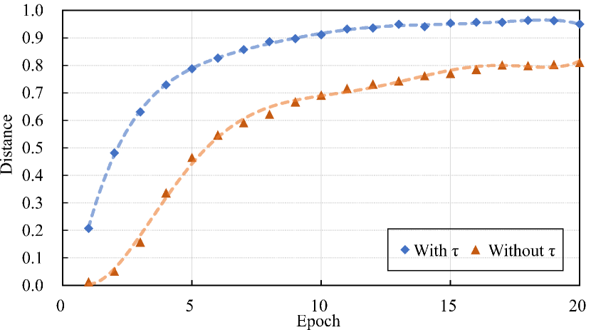
Figure 5: Comparisons of the discrepancy between the probabilities of positive and negative labels with or without ATC.

The original form of our PU loss in equation 11 would lead to over-smooth distributions in the early phase of training due to the learning difficulty. This small discrepancy between the probabilities of positive and negative samples would make the unlabeled term of PU loss hard to optimize. To alleviate the over-smooth problem, we propose adaptive temperature coefficient (ATC) to adjust the sharpness of distribution.

To prove that the ATC is beneficial to magnify the discrepancy of positive and negative samples, we measure the Kullback-Leibler divergence between the predicted probabilities of positive and negative labels in the first 20 epochs of training on 10% known label ratio. As shown in Figure 5, ATC can significantly enlarge the discrepancy between the predicted probabilities of positive and negative labels in the early stage of model training, thereby alleviating the over-smooth.

The formula of measuring discrepancy:

$$D_{KL}(P_{p}||P_{n})=\frac{1}{I\times C}\sum_{i=1}^{I}\sum_{c=1}^{C}P_{p}^{i,c}\log(\frac{P_{p}^{i,c}}{P_{n}^{i,c}}),$$ (16)

where $I$ denotes the number of iterations in an epoch. $P_{p}^{i,c}$ and $P_{n}^{i,c}$ denote average prediction probabilities of the positive and negative labels of category $c$ in the $i$-th iteration, respectively.

Appendix C More Ablation Studies

Effects of the exponential $\gamma$ in re-balance factor.

As shown in Table 6, we perform analysis of the exponential $\gamma$ on MS-COCO without adaptive temperature coefficient. Since there are far fewer positive labels than unknown labels at 10% proportion of known labels, the contribution of positive labels in training is heavily neglected under $\gamma$ = 0, leading to poor performance. When we fix $\gamma=0.3$, the above issue is significantly alleviated. However, as previously discussed, the degree of adjustment is individual under different proportions of known labels. In our setting, we set smaller $\gamma$ on larger proportions, allowing the model to achieve better performance.

Table 6: Comparisons of adopting different $\gamma$ in our loss.

Methods	10%	50%	90%
Fixed $\bm{\gamma}$ = 0	51.8	78.6	81.6
Fixed $\bm{\gamma}$ = 0.3	73.7	81.2	82.6
Our setting	74.3	81.3	83.4

Dropping Negative Labels or Positive Labels?

In this paper, we remove negative labels and use positive labels to conduct PU learning. While we can also remove positive labels and treat negative labels as “positive” in PU learning. To compare these two choices, we conduct experiments and report the results of dropping negative labels and dropping positive labels in Table 7. The results show that, dropping negative labels obtains obviously better performance. This imply that, the noisy labels in positive labels are fewer than that in negative labels, and we can achieve better performance on the cleaner positive labels, though the positive labels is much fewer than the negative ones.

Table 7: Comparisons of dropping positive or negative labels on MS-COCO and VOC. We report the mAP (%).

Dataset	MS-COCO	VOC 2007
Dropping positive	80.1	92.7
Dropping negative	82.8	93.8

Manually Adding Noisy Labels

In this paper, we aim to alleviate the influence of noisy labels in negative labels and introduce PU-MLC. However, COCO dataset is a finely annotated dataset and we cannot know how many labels are incorrect in it. To further validate our efficacy to different degrees of noisy ratios in dataset, we conduct experiments without LgConv to manually add noisy labels to the training dataset, and see how the noisy ratios affect the performance on PU-MLC and our BCE baseline. As shown in Table 8, we remove 10%, 50%, and 90% positive labels and labeled them as negatives, and therefore these new negative labels are false negative noises, we then train our PU-MLC and baseline BCE on these datasets. The results show that, the impact of noisy labels on our method is less than BCE at each noisy ratio. Particularly, with 90% positive labels shifted into noisy labels, the mAP is significantly dropped by 58.4% in BCE, while our PU-MLC only has a 8.1% reduction. This indicates that our method is more robust than the traditional PN-based method on noisy labels (false negative).

Table 8: Results of PU-MLC and BCE under different noisy label ratios. We report mAP (%) on COCO.

Methods	PU-MLC			BCE
	10%	50%	90%	10%	50%	90%
Original	83.6	83.6	83.6	80.0	80.0	80.0
Adding noise	83.2	81.5	75.5	79.3	74.5	21.6
Reduction	-0.4	-2.1	-8.1	-0.7	-5.5	-58.4

Effects of the Local-Global Convolution.

To validate the enhanced performance of LgConv on the backbone, we conduct ablation experiments across three distinct known label ratios on MS-COCO. The results, as shown in the Table 9, clearly demonstrate a noticeable improvement after integrating LgConv into the backbone. On average, there is a notable increase of 0.4 in mAP. Importantly, the implementation of LgConv does not necessitate retraining the backbone.

Table 9: Comparisons of backbone with and without LgConv on MS-COCO.

Methods	10%	50%	90%
Without LgConv	75.2	81.7	82.4
With LgConv	75.7	82.0	83.8

Effect of complementing $\mathcal{P}$ to $\mathcal{U}$.

We append all the samples in the positive set to the unlabeled set to obtain a similar label distribution to the original PN training dataset. To verify the effectiveness, we conduct experiments under three proportions of known labels to compare the performance with or without the complement. As shown in Table 10, the setting with 90% proportion of known labels obtains a relatively large improvement, while the gain on 10% proportion is small. The reason behind this is simple: when we have only a small portion (10%) of positive labels in the positive set, most of the remaining positive samples (90%) are in the unlabeled set, and thus the unlabeled set naturally holds a similar label distribution to the dataset. While on large portions, the label distribution in the unlabeled set is quite different to the origin (taking an extreme 100% portion as an example, there are no positive samples in the unlabeled set).

Table 10: Results of adding or not adding $\mathcal{P}$ to $\mathcal{U}$ on COCO.

Methods	10%	50%	90%
Not adding $\mathcal{P}$ to $\mathcal{U}$	75.5	81.7	82.7
Adding $\mathcal{P}$ to $\mathcal{U}$	75.7	82.0	83.8

Ablation studies on hyper-parameters $\lambda$ and $\alpha$.

We conduct an analysis on the Pascal VOC dataset to examine the influence of hyper-parameters, specifically $\lambda$ and $\alpha$, on PU-MLC. Figure 6(a) demonstrates that our method shows insensitivity to changes in $\lambda$, with the mAP fluctuating between 87.5% and 88.0%. Therefore, we opt to select the $\lambda$ value of 1.0 that yields the best performance as our experimental setting. Additionally, Figure 6(b) illustrates that both large and small $\alpha$ values have a negative impact on the model. Particularly, when $\alpha$ exceeds 5.5, the mAP decreases by 1.1%. Consequently, we chose the $\alpha$ value of 2.0 as our experimental setting, as it yields the best performance.

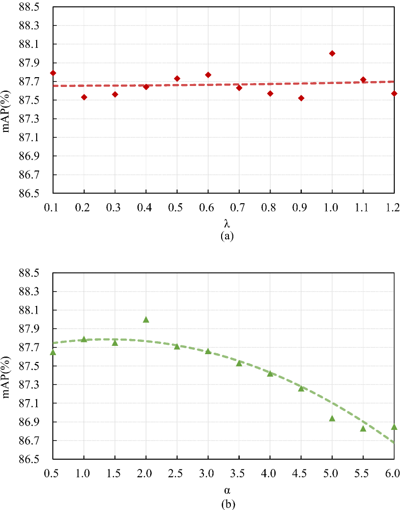
Figure 6: Ablation on hyper-parameters $\lambda$ and $\alpha$. We report the mAP (%) of different $\lambda$ and $\alpha$ at the 10% known label ratio.

Ablation studies on exponential $\gamma$ selection.

In Table 6, we elaborate on the importance of dynamically selecting the $\gamma$ for each known label ratio. Figure 7 visualizes the process of $\gamma$ selection at 10% and 50% known label ratios on Pascal VOC. It is crucial to choose an appropriate $\gamma$ to ensure the re-balance factor adequately balances the contributions of positive and unknown labels during training. On the contrary, improper $\gamma$ leads to suboptimal performance of the re-balance factor. To address this, we carefully choose the $\gamma$ that yields the best performance at each known label ratio.

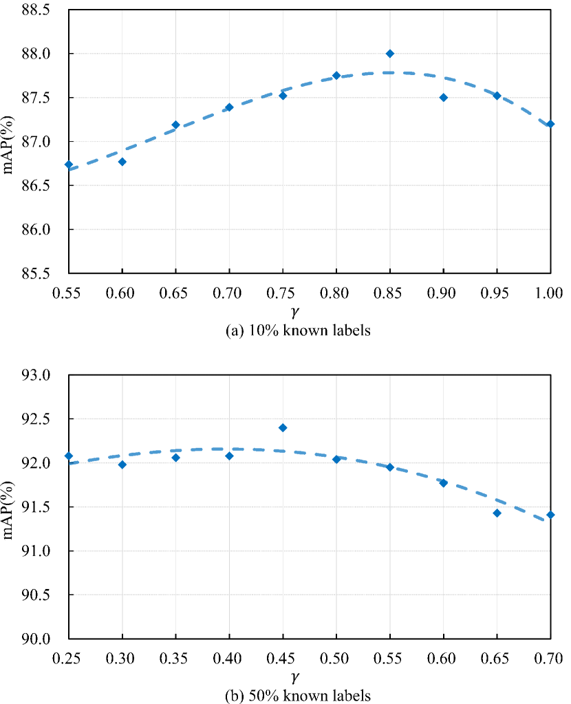
Figure 7: Ablation studies on exponential $\gamma$ selection. We report the mAP (%) of different $\gamma$ on VOC 2007.

Freezing BatchNorm Stats

In MLC task, the backbone is initialized with weights pretrained on ImageNet dataset. Current methods usually set the BatchNorm (BN) layers into train mode and update the running mean and standard deviation values with MLC datasets. However, we find that this strategy may not be the optimal in our method. As summarized in Table 11, we train our model with and without freezing the stats in BNs, and the results show that, when the known label ratio is high (100%), the traditional not freezing BN obtains slightly higher mAP, while on smaller ratios especially 10%, freezing BN achieves significant improvements. This implies that, when with smaller known label ratios, the model is more sensitive and updating BN stats with the training dataset may make this situation severer, while fixing the BN stats (set to eval mode) could result in stabler optimization. As a result, we fix the BN stats in all the experiments of our PU-MLC.

Table 11: Comparisons of mAPs of freezing and not freezing BatchNorm stats on MS-COCO.

Methods	10%	50%	100%
Not freezing BN	74.6	81.9	84.4
Freezing BN	75.7	82.0	84.2

Compare with CSL

Due to a distinct strategy employ by CSL (Ben-Baruch et al. 2022) in making partial label datasets and its utilization of a unique backbone, a fair comparison between CSL and other methods in Table 1 of the paper is not feasible. We conduct experiments to use the same training settings in our method. Concretely, we employ the fixed per class (FPC) of 1000 strategy to generate a partial label dataset and use the TResNet-M (Ridnik et al. 2021b) as the backbone. As shown in Table 12, our PU-MLC obtains 85.4% mAP, significantly outperforming CSL.

Table 12: Compared with CSL on MS-COCO.

Methods	FPC=1000
CSL	83.4
PU-MLC	85.4

References

- Bekker and Davis (2020) Bekker, J.; and Davis, J. 2020. Learning from positive and unlabeled data: a survey. Machine Learning, 719–760.
- Ben-Baruch et al. (2022) Ben-Baruch, E.; Ridnik, T.; Friedman, I.; Ben-Cohen, A.; Zamir, N.; Noy, A.; and Zelnik-Manor, L. 2022. Multi-label classification with partial annotations using class-aware selective loss. In Proceedings of the IEEE/CVF Conference on Computer Vision and Pattern Recognition, 4764–4772.
- Chang, Du, and Zhang (2021) Chang, S.; Du, B.; and Zhang, L. 2021. Positive unlabeled learning with class-prior approximation. In Proceedings of the Twenty-Ninth International Conference on International Joint Conferences on Artificial Intelligence, 2014–2021.
- Chen et al. (2020) Chen, H.; Liu, F.; Wang, Y.; Zhao, L.; and Wu, H. 2020. A Variational Approach for Learning from Positive and Unlabeled Data. In Advances in Neural Information Processing Systems, 14844–14854.
- Chen et al. (2022a) Chen, T.; Lin, L.; Chen, R.; Hui, X.; and Wu, H. 2022a. Knowledge-guided multi-label few-shot learning for general image recognition. IEEE Transactions on Pattern Analysis and Machine Intelligence, 44(3): 1371–1384.
- Chen et al. (2022b) Chen, T.; Pu, T.; Wu, H.; Xie, Y.; and Lin, L. 2022b. Structured Semantic Transfer for Multi-Label Recognition with Partial Labels. In Proceedings of the AAAI conference on artificial intelligence, 339–346.
- Chen et al. (2019a) Chen, T.; Xu, M.; Hui, X.; Wu, H.; and Lin, L. 2019a. Learning Semantic-Specific Graph Representation for Multi-Label Image Recognition. In Proceedings of the IEEE/CVF International Conference on Computer Vision (ICCV), 522–531.
- Chen et al. (2021) Chen, Z.; Wei, X.-S.; Wang, P.; and Guo, Y. 2021. Learning graph convolutional networks for multi-label recognition and applications. IEEE Transactions on Pattern Analysis and Machine Intelligence.
- Chen et al. (2019b) Chen, Z.-M.; Wei, X.-S.; Jin, X.; ; and Guo, Y. 2019b. Multi-label image recognition with joint class-aware map disentangling and label correlation embedding. In 2019 IEEE International Conference on Multimedia and Expo (ICME), 622–627.
- Chen et al. (2019c) Chen, Z.-M.; Wei, X.-S.; Wang, P.; and Guo, Y. 2019c. Multi-Label Image Recognition With Graph Convolutional Networks. In Proceedings of the IEEE/CVF Conference on Computer Vision and Pattern Recognition (CVPR), 5177–5186.
- Deng et al. (2009) Deng, J.; Dong, W.; Socher, R.; Li, L.-J.; Li, K.; and Fei-Fei, L. 2009. ImageNet: A large-scale hierarchical image database. In 2009 IEEE conference on computer vision and pattern recognition, 248–255.
- Dosovitskiy et al. (2020) Dosovitskiy, A.; Beyer, L.; Kolesnikov, A.; Weissenborn, D.; Zhai, X.; Unterthiner, T.; Dehghani, M.; Minderer, M.; Heigold, G.; Gelly, S.; et al. 2020. An Image is Worth 16x16 Words: Transformers for Image Recognition at Scale. In International Conference on Learning Representations.
- Durand, Mehrasa, and Mori (2019) Durand, T.; Mehrasa, N.; and Mori, G. 2019. Learning a Deep ConvNet for Multi-Label Classification With Partial Labels. In Proceedings of the IEEE/CVF Conference on Computer Vision and Pattern Recognition (CVPR), 647–657.
- Everingham et al. (2010) Everingham, M.; Gool, L. V.; Williams, C. K. I.; Winn, J.; and Zisserman, A. 2010. The pascal visual object classes (voc) challenge. International journal of computer vision, 88(2): 303–338.
- Gong et al. (2021) Gong, C.; Wang, Q.; Liu, T.; Han, B.; You, J.; Yang, J.; and Tao, D. 2021. Instance-dependent positive and unlabeled learning with labeling bias estimation. IEEE Transactions on Pattern Analysis and Machine Intelligence, 44(8): 4163–4177.
- He et al. (2016) He, K.; Zhang, X.; Ren, S.; and Sun, J. 2016. Deep Residual Learning for Image Recognition. In Proceedings of the IEEE conference on computer vision and pattern recognition, 770–778.
- Hinton, Vinyals, and Dean (2015) Hinton, G.; Vinyals, O.; and Dean, J. 2015. Distilling the knowledge in a neural network. arXiv:1503.02531.
- Hu et al. (2021) Hu, W.; Le, R.; Liu, B.; Ji, F.; Ma, J.; Zhao, D.; and Yan, R. 2021. Predictive adversarial learning from positive and unlabeled data. In Proceedings of the AAAI Conference on Artificial Intelligence, volume 35, 7806–7814.
- Huang et al. (2022a) Huang, T.; You, S.; Wang, F.; Qian, C.; and Xu, C. 2022a. Knowledge Distillation from A Stronger Teacher. In Advances in Neural Information Processing Systems, 33716–33727.
- Huang et al. (2022b) Huang, T.; You, S.; Wang, F.; Qian, C.; Zhang, C.; Wang, X.; and Xu, C. 2022b. Greedynasv2: Greedier search with a greedy path filter. In Proceedings of the IEEE/CVF Conference on Computer Vision and Pattern Recognition, 11902–11911.
- Huang et al. (2022c) Huang, T.; You, S.; Zhang, B.; Du, Y.; Wang, F.; Qian, C.; and Xu, C. 2022c. Dyrep: Bootstrapping training with dynamic re-parameterization. In Proceedings of the IEEE/CVF Conference on Computer Vision and Pattern Recognition, 588–597.
- Huynh and Elhamifar (2020) Huynh, D.; and Elhamifar, E. 2020. Interactive multi-label cnn learning with partial labels. In Proceedings of the IEEE/CVF Conference on Computer Vision and Pattern Recognition (CVPR), 9423–9432.
- Kingma and Ba (2014) Kingma, D. P.; and Ba, J. 2014. Adam: A Method for Stochastic Optimization. arXiv:1412.6980.
- Kipf and Welling (2016) Kipf, T. N.; and Welling, M. 2016. Semi-Supervised Classification with Graph Convolutional Networks. arXiv:1609.02907.
- Kiryo et al. (2017) Kiryo, R.; Niu, G.; du Plessis, M. C.; and Sugiyama, M. 2017. Positive-Unlabeled Learning with Non-Negative Risk Estimator. In Advances in neural information processing systems, 1675–1685.
- Lanchantin et al. (2021) Lanchantin, J.; Wang, T.; Ordonez, V.; and Qi, Y. 2021. General Multi-Label Image Classification With Transformers. In Proceedings of the IEEE/CVF Conference on Computer Vision and Pattern Recognition (CVPR), 16478–16488.
- Lin et al. (2017) Lin, T.-Y.; Goyal, P.; Girshick, R.; He, K.; and Dollár, P. 2017. Focal loss for dense object detection. In Proceedings of the IEEE international conference on computer vision, 2980–2988.
- Lin et al. (2014) Lin, T.-Y.; Maire, M.; Belongie, S.; Hays, J.; Perona, P.; Ramanan, D.; Dollár, P.; and Zitnick, C. L. 2014. Microsoft COCO: Common Objects in Context. In European conference on computer vision, 740–755.
- Liu et al. (2021) Liu, Z.; Lin, Y.; Cao, Y.; Hu, H.; Wei, Y.; Zhang, Z.; Lin, S.; and Guo, B. 2021. Swin transformer: Hierarchical vision transformer using shifted windows. In Proceedings of the IEEE/CVF international conference on computer vision, 10012–10022.
- Plessis, Niu, and Sugiyama (2015) Plessis, M. D.; Niu, G.; and Sugiyama, M. 2015. Convex Formulation for Learning from Positive and Unlabeled Data. In International conference on machine learning, 1386–1394.
- Pu et al. (2022) Pu, T.; Chen, T.; Wu, H.; Lu, Y.; and Lin, L. 2022. Semantic-Aware Representation Blending for Multi-Label Image Recognition with Partial Labels. arXiv:2205.13092.
- Radford et al. (2021) Radford, A.; Kim, J. W.; abd Aditya Ramesh, C. H.; Goh, G.; Agarwal, S.; Sastry, G.; Askell, A.; Mishkin, P.; Clark, J.; Krueger, G.; and Sutskever, I. 2021. Learning transferable visual models from natural language supervision. In International conference on machine learning, 8748–8763.
- Ridnik et al. (2021a) Ridnik, T.; Ben-Baruch, E.; Zamir, N.; Noy, A.; Friedman, I.; Protter, M.; and Zelnik-Manor, L. 2021a. Asymmetric loss for multi-label classification. In Proceedings of the IEEE/CVF International Conference on Computer Vision, 82–91.
- Ridnik et al. (2021b) Ridnik, T.; Lawen, H.; Noy, A.; Baruch, E. B.; Sharir, G.; and Friedman, I. 2021b. Tresnet: High performance gpu-dedicated architecture. In proceedings of the IEEE/CVF winter conference on applications of computer vision, 1400–1409.
- Simonyan and Zisserman (2014) Simonyan, K.; and Zisserman, A. 2014. Very Deep Convolutional Networks for Large-Scale Image Recognition. arXiv:1409.1556.
- Smith (2018) Smith, L. N. 2018. A disciplined approach to neural network hyper-parameters: Part 1 – learning rate, batch size, momentum, and weight decay. arXiv:1803.09820.
- Sun, Hu, and Saenko (2022) Sun, X.; Hu, P.; and Saenko, K. 2022. Dualcoop: Fast adaptation to multi-label recognition with limited annotations. arXiv:2206.09541.
- Szegedy et al. (2016) Szegedy, C.; Vanhoucke, V.; Ioffe, S.; Shlens, J.; and Wojna, Z. 2016. Rethinking the Inception Architecture for Computer Vision. In Proceedings of the IEEE conference on computer vision and pattern recognition, 2818–2826.
- Thyagarajan et al. (2022) Thyagarajan, A.; Snorrason, E.; Northcutt, C.; and Mueller, J. 2022. Identifying Incorrect Annotations in Multi-Label Classification Data. arXiv:2211.13895.
- You et al. (2020) You, R.; Guo, Z.; Cui, L.; Long, X.; Bao, Y.; and Wen, S. 2020. Cross-Modality Attention with Semantic Graph Embedding for Multi-Label Classification. Proceedings of the AAAI conference on artificial intelligence, 34(7): 12709–12716.
- Zhang et al. (2017) Zhang, H.; Cisse, M.; Dauphin, Y. N.; and Lopez-Paz, D. 2017. mixup: Beyond empirical risk minimization. arXiv:1710.09412.
- Zhao et al. (2021) Zhao, J.; Yan, K.; Zhao, Y.; Guo, X.; Huang, F.; and Li, J. 2021. Transformer-based Dual Relation Graph for Multi-label Image Recognition. In Proceedings of the IEEE/CVF International Conference on Computer Vision (ICCV), 163–172.