Collective Wigner crystal tunneling in carbon nanotubes

Abstract

The collective tunneling of a a Wigner necklace – a crystalline state of a small number of strongly interacting electrons confined to a suspended nanotube and subject to a double well potential – is theoretically analyzed and compared with experiments in [Shapir et al., Science 364, 870 (2019)]. Density Matrix Renormalization Group computations, exact diagonalization, and instanton theory provide a consistent description of this very strongly interacting system, and show good agreement with experiments. Experimentally extracted and theoretically computed tunneling amplitudes exhibit a scaling collapse. Collective quantum fluctuations renormalize the tunneling, and substantially enhance it as the number of electrons increases.

I Introduction

While investigating correlation effects in electron liquids, Eugene Wigner conjectured in 1934 the existence of an electron crystal [1], today referred to as the Wigner crystal. In his seminal work, Wigner noticed that the interaction energy of a three-dimensional electron gas scales as $E_{\text{int}}\sim n^{1/3}$ with their density $n$, and dominates over the kinetic energy $E_{K}\sim n^{2/3}$ in the very dilute limit. Therefore, electrons must become localized at very small carrier concentrations, and form a crystal. The kinetic energy of the electrons increases upon compression, and the crystal melts due to quantum and thermal fluctuations into an electron liquid. A similar solid–liquid (quantum) phase transition occurs in two spatial dimensions. In one dimension, however, quantum fluctuations always destroy long-range order, and no phase transition takes place: only a cross-over between a Luttinger liquid-like and a dilute regime with power-law crystalline correlations appears [2].

Since the predictions of Wigner, tremendous effort has been devoted to detect and understand this quantum crystal. While these efforts remained unsuccessful in three dimensions, Wigner crystal phases and correlations have been demonstrated in two-dimensional structures  [3, 4, 5, 6, 7, 8, 9, 10, 11, 12, 13, 14, 15, 16, 17, 18, 19, 20, 21, 22] as well as more recently in one dimension [23, 24].

In particular, in Ref. [23] the real space structure of a small one-dimensional crystal in a carbon nanotube has been carefully probed, and the collective tunneling of the crystal observed. In this work, we focus on this latter phenomenon, and model and analyze the tunneling of a small, one-dimensional Wigner crystal.

The set-up of Ref. [23] is displayed in Fig.1(a). A carbon nanotube is suspended and gated appropriately. Gates on the r.h.s., underneath the nanotube are used to trap $N$ electrons (or holes), and to create a confining potential $V(z)$ at wish, with $z$ the electrons’ coordinate along the nanotube. On the left, a quantum dot is created from the very same nanotube, and used as a charge detector. The spatial structure of charge distributions within the nanotube can further be detected by placing a probe nanotube on the top of the device, and measuring the charge detector’s response.

The confining potential $V(z)$ is well approximated by a simple quartic form,

$$V(z)={b\over 4}z^{4}-{a\over 2}z^{2}-c\,z,$$ (1)

with $a$, $b$ and $c$ tunable parameters. Tunneling between the two sides of the potential is generated by applying a bias and thereby changing the sign of $c$.

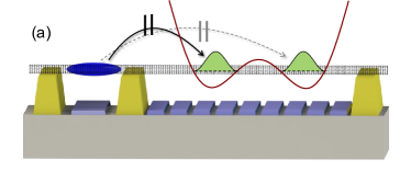
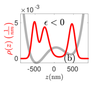
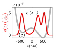
Figure 1: (a) Experimental setup of Ref. [23] used to detect collective tunneling. The bottom gates under the nanotube are used to shape the double well potential, the left-hand-side quantum dot (dark blue) serves as a charge detector. (b) and (c) Ground state charge densities (red) from exact diagonalization for a system of three electrons in a double well potential (grey). A single electron moves between the two sides upon changing the asymmetry. The charge density displays a crystalline structure due to the strong Coulomb interaction ($\eta=20$ in Eq. (7)) .

In the present work we investigate theoretically the collective tunneling of strongly interacting charged particles in the potential $V(z)$. Such collective tunneling occurs for an odd number of particles. Then the classical ground state of the particles is twofold generated in a symmetrical potential, but quantum tunneling allows for the hybridization of these two states, and splits their energy. However, as demonstrated experimentally [23], due to the strong Coulomb interaction, moving just one charge from one side of the barrier to the other is accompanied by the reordering of charges and a collective motion of all particles.

The theoretical study of this phenomenon is rather challenging in the strongly interacting regime, where usual quantum chemistry approaches break down [25]. We apply a combination of three different methods. In the deep tunneling regime an instanton approach can be used [26]. Incorporating quantum fluctuations turns out to be crucial (as well as a technical challenge) in the quantum tunneling regime. Unfortunately, most of the experimental data turn out to be in the intermediate region, where instanton theory is inapplicable. To capture the physics in this regime, too, we perform (restricted) exact diagonalization calculations and compare these with Density Renormalization Group (DMRG) based computations. These three approaches provide us a consistent picture, confirm the presence of collective tunneling, and are in good agreement with the experimental data.

The paper is organized as follows: In Section II we outline the basic model used to describe the experimental setup of Ref. [23]. Section III is devoted to the discussion of the three complementary theoretical methods used in this work. Our results are presented in Section IV, along with a detailed comparison with the experimental data. Our conclusions are summarized in Section V, while some technical details of the instanton calculation are described in Appendix A.

II Modelling the experimental setup

To observe the Wigner crystal regime in a carbon nanotube, the mass of the charge carriers needs to be as large as possible, and their interaction as strong as possible. The Wigner crystal regime is therefore ideally observed in suspended small diameter semiconducting nanotubes with large gaps, as the ones used in Refs. [23, 24]. Electrons confined to such nanotubes are very well described by the effective Hamiltonian

$$H=\sum_{i=1}^{N}\left[-\frac{\hbar^{2}}{2m^{*}}\frac{\partial^{2}}{\partial z_{i}^{2}}+V(z_{i})\right]+\sum_{i<j}^{N}\frac{e^{2}}{4\pi\varepsilon_{0}}\frac{1}{\left|z_{i}-z_{j}\right|},$$ (2)

with $m^{*}$ the effective mass of the electrons (holes) in the nanotube, and $V(z)$ the confining potential, Eq. (1). The spin $\sigma$ and the chirality $\tau$ of the particles do not appear in this Hamiltonian [27]. They play an important role at larger electron densities [28]. However, since the tunneling experiments studied here and in Ref. [23] are performed in the spin incoherent regime [29], here we neglect them, and consider simply interacting spinless fermions. We also disregard the impact of spin-orbit interaction, having a mild effect on the measured charge densities or the interaction energies. These, however, modify the structure of spin excitations at very low temperatures or in the cross-over regime, where the Wigner starts to melt and the role of exchange interaction becomes important [28].

Usually, the strength of electron-electron interaction in a homogeneous, $d$-dimensional electron gas is characterized by the parameter $r_{s}=n^{-1/d}/a_{B}$, the ratio of the typical distance between charge carriers and the Bohr radius, $a_{B}=\hbar^{2}\varepsilon/me^{2}$. At $r_{s}\approx 1$ the electrons’ kinetic energy is approximately the same as their potential energy, while for $r_{s}\gg 1$ the interaction energy dominates. It is in the latter regime that the Wigner crystal emerges.

In a confined potential, however, the concept of $r_{s}$ is not particularly useful. There the confining potential sets a typical length scale, which in our case is simply the oscillator length of the quartic potential ($a=c=0$),

$$l_{d}=\left(\frac{\hbar^{2}}{m^{*}b}\right)^{1/6}.$$ (3)

Introducing the corresponding dimensionless coordinates, $z\to\chi=z/l_{d}$, defines then the natural energy scale of the problem,

$$E_{0}=\frac{\hbar^{2}}{m^{*}l_{d}^{2}}\;,$$ (4)

and leads to the definition of the dimensionless strength of the Coulomb interaction,

$$\eta=\frac{l_{d}}{a_{B}}=\frac{m^{*}e^{2}}{\varepsilon\,\hbar^{2}}\left(\frac{\hbar^{2}}{m^{*}b}\right)^{1/6}.$$ (5)

For the nanotube investigated here and in Ref. [23] we obtain

$$l_{d}\approx 160\,{\rm{nm}},\phantom{22}E_{0}\approx 5.56\,{\rm{K}},\phantom{22}\eta\approx 20,$$ (6)

the latter signaling an extremely strong Coulomb interaction.

In terms of these units, we obtain the dimensionless Hamiltonian

$$\tilde{H}=\sum_{i=1}^{N}\left[-\frac{1}{2}\frac{\partial^{2}}{\partial\chi_{i}^{2}}+\frac{1}{4}\chi_{i}^{4}-\frac{\alpha}{2}\chi_{i}^{2}-\epsilon\chi_{i}\right]+\eta\sum_{i<j}^{N}\frac{1}{\left|\chi_{i}-\chi_{j}\right|},$$ (7)

where the dimensionless parameter $\alpha=a\,l_{d}^{2}/E_{0}$ sets the height of the tunneling barrier between the two valleys, while $\epsilon=c\,l_{d}/E_{0}$ characterizes their bias.

III Theoretical approaches

Our goal is to compute the tunneling amplitude $\Delta$ of the crystal, i.e., the splitting of the two almost degenerate states for $N=\text{odd}$, and to investigate this tunnel splitting and the electrons’ charge distribution as a function of the potential height $\alpha$, and the bias $\epsilon$. The tunneling amplitude is inversely proportional to the polarizability of the Wigner crystal at $T=0$ temperature, and is therefore directly accessible experimentally via polarization measurements, while charge distributions can be detected by an AFM-like method using a probe nanotube [23].

III.1 Instanton theory

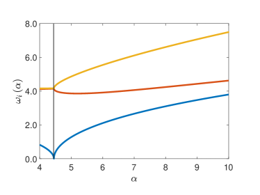
Figure 2: Soft modes $\omega_{i}$ as a function of $\alpha$, for $N=3$. The vertical line at $\alpha=\alpha_{cr}\approx 4.45$ marks the beginning of the tunneling regime. For $\alpha>\alpha_{cr}$ there are two independent equilibrium position, while for $\alpha<\alpha_{cr}$ only one, indicating the absence of the tunneling at small $\alpha$.

We first consider the Wigner crystal tunneling problem by using the instanton approach [30, 31, 32, 33, 26]. Instanton theory (IT) is accurate in the tunneling regime, $\alpha\gg 0$, however, it breaks down at small positive values, $\alpha\lesssim\alpha_{\text{cr}}$, with $\alpha_{\text{cr}}$ denoting the barrier height parameter, where tunneling sets in.

In the instanton approach, one considers the imaginary time tunneling amplitude between two many-body positions. Tunneling appears as a classical motion of the particles in imaginary time, and the tunneling amplitude is proportional to $\Delta\sim e^{-S_{\text{inst}}}$, with $S_{\text{inst}}$ the instanton action. Fluctuations around this classical path determine the amplitude of tunneling, i.e., the prefactor in front of the exponential [30].

The energy splitting $\Delta$ of the lowest lying states can be obtained by computing the imaginary time Feynman propagator, between the minima $\mathbold{\chi}_{0}$ and $\mathbold{\chi}_{0}^{\prime}$ of the many-body potential,

$$v_{N}(\bm{\chi})=\sum_{i=1}^{N}\left(-\frac{\alpha}{2}\chi_{i}^{2}+\frac{1}{4}\chi_{i}^{4}\right)+\eta\sum_{i<j}^{N}\frac{1}{|\chi_{i}-\chi_{j}|},$$ (8)

with ${\tau}$ the dimensionless imaginary propagation time measured in units of $\hbar/E_{0}$. One can express (LABEL:eq:Feynman) as a path integral in terms of the imaginary time trajectories, $\mathbold{\chi}({\tau})$, which are separated into a classical instanton trajectory, $\bm{\chi}_{\text{cl}}({\tau})$, minimizing the classical (Euclidean) action

$$S_{E}[\bm{\chi}({\tau})]=S_{0}\int_{0}^{T}{\rm{d}}{\tau}\Big{\{}{1\over 2}\sum_{i=1}^{N}\Big{(}\frac{{\rm{d}}\chi_{i}}{{\rm{d}}{\tau}}\Big{)}^{2}+v_{N}(\bm{\chi})\Big{\}}.$$ (9)

and small fluctuations around that, $\bm{\chi}({\tau})=\bm{\chi}_{\text{cl}}({\tau})+\mathbf{r}({\tau})$. The prefactor $S_{0}=(l_{d}/E_{0})^{3/2}$ emerges naturally, and denotes the natural action unit in this problem, and ${T}$ denotes the tunneling time in units of $\hbar/E_{0}$. Expanding the action to second order in $\mathbf{r}(\tau)$ leads to the expression

$$K(\bm{\chi}_{0}^{\prime},\bm{\chi}_{0},T)\approx e^{-S_{\text{inst}}}\int_{\mathbf{r}(0)=0}^{\mathbf{r}(T)=0}{\cal D}\mathbf{r}\exp\Big{\{}\frac{1}{2}\int_{0}^{T}{\rm{d}}{\tau}\,\mathbf{r}({\tau})\cdot$$

$$\left[-\partial^{2}_{{\tau}}+\partial\circ\partial\,v_{N}(\bm{\chi}_{cl}({\tau}))\right]\mathbold{r}({\tau})\Big{\}},$$ (10)

with $S_{\text{inst}}=S_{E}[\bm{\chi}_{\text{cl}}({\tau})]$ the instanton action, and the integral accounting for quantum fluctuations around it.

We determined the initial and final equilibrium positions $\bm{\chi}_{0}$ and $\bm{\chi}_{0}^{\prime}$ as well as the instanton trajectories by applying a Monte Carlo simulated annealing procedure [34]. Fig. 2 shows the frequencies of small vibrations around the minimum (minima) of $v_{N}(\bm{\chi})$ for $N=3$. The symmetrical position of the three particles becomes classically unstable at $\alpha^{N=3}_{\text{cr}}\approx{4.45}$, the classical threshold for collective tunneling. For $\alpha<\alpha_{\text{cr}}$ the minimum energy configuration is unique, while for $\alpha>\alpha_{\text{cr}}$ two equilibrium positions exist, and tunneling becomes possible. The transition to the tunneling regime is marked by the softening of the lowest energy mode. Interestingly, the direction of this mode coincides with that of the instanton trajectory for $\alpha>\alpha_{\text{cr}}$.

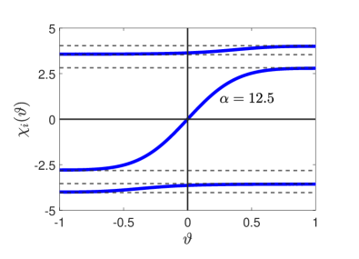
Figure 3: Three particle imaginary time trajectories (blue) in the dimensionless units for a specific confinement parameter $\alpha=12.5>\alpha_{\text{cr}}$ and $\eta=20$. Dashed lines show the classical equilibrium positions or instanton turning points for the 3 particles.

A typical trajectory is displayed for $N=3$ particles in Fig. 3, which demonstrates collective tunneling. In our calculations, we ”compactify” time by introducing the parameter $\vartheta=\tanh({{\tau}}/{{\tau}_{0}})$, and parametrize $\bm{\chi}$ by using $\vartheta$. Clearly, the middle electron tunnels through the potential barrier, while the outer electrons do not tunnel but adjust their positions.

The choice of ${\tau}_{0}$ is important from the point of view of numerical accuracy. A small value of ${\tau}_{0}$ increases the numerical accuracy in the tunneling region, while a large value of ${\tau}_{0}\approx 5$ provides better resolution around the end of the trajectories. Since the primary contribution to the energy splitting arises from the region around ${\tau}\approx 0$, a value ${\tau}_{0}\approx 0.5$ turns out to be optimal for accurate calculations.

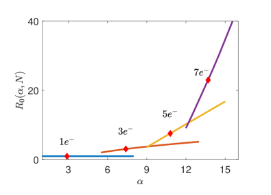
Figure 4: Renormalization factor $R_{0}(\alpha,N)$ as function of $\alpha$ for $N\in\{1,3,5,7\}$. On each line, the diamond symbols mark the beginning of the quantum tunneling regime.

Performing the Gaussian integral in Eq. (10) is a highly non-trivial task [35, 26]. The procedure consists of introducing the arc length variable ${\rm d}s^{2}={\rm d}\bm{\chi}_{\text{cl}}^{2}$ along the instanton trajectory, and $N-1$ perpendicular coordinates. In this way, one describes the tunneling as a one-dimensional tunneling process in an effective potential $w(s)$, renormalized by ’perpendicular’ quantum fluctuations (see Apendix A). The tunneling amplitude is then expressed as

$$\Delta = R_{0}(\alpha,N)\,\Delta_{1}\,,$$

$$\Delta_{1} = \sqrt{\frac{4\omega_{\rm{soft}}}{\pi}}\sqrt{2[v_{N}^{\rm{max}}-v_{N}^{\rm{min}}]}P[{\mathbold{\chi}}_{cl}(s)]e^{-S_{E}},$$ (11)

with $\Delta_{1}$ associated with a one-dimensional motion in the effective double-well potential, and $R_{0}(\alpha,N)$ the aforementioned renormalization factor [35, 26] (see Appendix  A for details). Here $\omega_{\rm{soft}}$ denotes the oscillation frequency at the initial position of the tunneling trajectory in the tunneling direction, and $P\left[\mathbold{\chi}_{\text{cl}}\right]$ is a renormalization factor associated with the effective one-dimensional motion. The prefactor $R_{0}$ is equal to 1 for $N=1$, but it becomes significant for $N\geq 3$ (see Fig. 4), and exhibits a non-negligible $\alpha$ dependence. Somewhat surprisingly, quantum fluctuations seem to increase the tunneling amplitude substantially, and quantitative computations must take them into account.

III.2 Density matrix renormalization group

As an alternative to instanton computations, we also performed density matrix renormalization group (DMRG) computations. DMRG provides an accurate description of the intermediate tunneling regime, however, it fails in the deep tunneling regime, where we experience convergence problems.

Originally, DMRG has been proposed as an efficient computational scheme for one-dimensional systems with short-ranged interactions  [36], but has been extended later to systems with long-ranged interactions as well as to higher dimensional lattices [37], and it has been reformulated more recently in a possibly more transparent way by using the language of matrix product states (MPS’s) [38, 39].

To perform DMRG, we express the Hamiltonian (7) in a second quantized form. The key to efficient DMRG calculations is to choose an appropriate basis in the strongly interacting limit studied here, $\eta\gg 1$. The most natural choice of harmonic oscillator basis functions centered at $\chi=0$, e.g., is not able to reach this regime [25]. Here we perform calculations by using an overcomplete adaptive basis with harmonic oscillator wave functions localized around the classical equilibrium positions of the electrons [23].

In this basis, we rewrite the Hamiltonian (7) the second quantized form

$$\tilde{H}=\sum_{a,b}t_{ab}c^{\dagger}_{a}c_{b}+{1\over 2}\sum_{a,b,c,d}V_{ab,cd}c^{\dagger}_{a}c^{\dagger}_{b}c_{d}c_{c},$$ (12)

where $t_{ab}$ stands for the matrix elements of the non-interacting part of (7), $t_{ab}=\langle\psi_{a}|\tilde{H}_{0}|\psi_{b}\rangle$, while $V_{ab,cd}=\langle\psi_{a}\psi_{b}|U|\psi_{c}\psi_{d}\rangle$ are the matrix elements of the Coulomb interaction, $U=\eta/|\chi-\chi^{\prime}|$ calculated within the single particle wave functions described above. The computation of the matrix elements $V_{ab,cd}$ is numerically demanding, but it can be speeded up by exploiting the translational invariance of the Coulomb interaction.

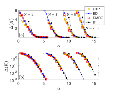
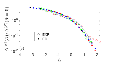
Figure 5: (a,b) Numerically computed tunnel splitting on both linear and logarithmic scales, compared with the rescaled experimental polarization data (EXP). Instanton theory captures $\Delta$ accurately in the deep tunneling regime, where $\Delta$ is suppressed exponentially by increasing barrier height (see panel (b)). Each set of curves corresponds to a different number of electrons, $N$. In panel (c), the data are scaled together and trace a single, universal curve. The tunneling regime starts at $\tilde{\alpha}\approx 0$.

For our computations, we utilized the Budapest-DMRG code [40, 41, 42], which allows us to treat long-range interactions efficiently and to take advantage of the $U(1)$ symmetry of the model associated with the conservation of the total charge as well as the $Z_{2}$ symmetry associated with parity. In our computations, we use a bond dimension of the order of 2048-4096, and an adaptive basis consisting of $8-16$ orbitals/electron, depending on the number of electrons. We computed the ground state energies in the even and odd parity sectors, $E_{GS}^{(e)}$ and $E_{GS}^{(o)}$, and extracted the energy splitting

$$\Delta=|E_{GS}^{(e)}-E_{GS}^{(o)}|,$$ (13)

identified as twice the tunneling amplitude in the tunneling regime. Typical results for $\Delta$ as well as a comparison with the results of the other approaches we used are displayed in Fig. 5 as function of $\alpha$. Unfortunately, in the deep tunneling regime, where $\Delta$ becomes exponentially small, $\Delta\lesssim 10^{-3}$, we noticed that the convergence of DMRG was influenced by the choice of basis we utilized. Specifically, as we decreased $\alpha$, the states became increasingly localized, which led to convergence challenges for the desired accuracy. Although increasing the bond dimensions improves the calculations, it also demanded greater computational resources. Consequently, as an alternative approach, we employed complementary methods like restricted exact diagonalization or instanton theory to achieve accurate results. Nevertheless, the range of applicability of DMRG overlaps with that of these methods, and enables us to obtain a complete description of the collective tunneling.

III.3 Restricted Exact Diagonalization

As a third, complementary method, we also used the restricted exact diagonalization (ED), which can be utilized to determine the eigenstates of relatively small quantum systems. Here we also use it to benchmark the other two, more sophisticated methods. In this work, we diagonalize the Hamiltonian (7) in real space.

For $N\in\{1,3\}$, diagonalization is performed with a relatively large number of states, $\sim 100$ for each particle, ensuring accurate ground state and a few excited state energies. However, for $N\in\{5,7\}$, the Hilbert space becomes too large, and a complete diagonalization is impossible in practice. Nevertheless, a projected version of ED can be used even in these cases, where a restricted wave function is used, with electrons treated as distinguishable particles. This method reduces the size of the Hilbert space by 2-3 orders of magnitude, and can be used to study up to $N=7$ electrons the low-energy spectrum in the strongly interacting limit, where exchange processes are unimportant [43].

IV Results and comparison with experimental data

IV.1 Polarization, polarizability, and tunneling amplitude

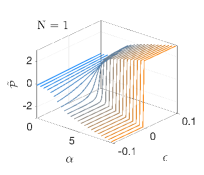
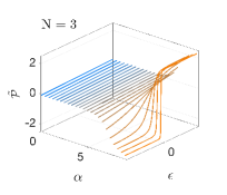
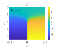
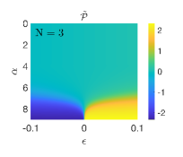
Figure 6: Density plots for the charge polarization $\tilde{P}(\alpha,\epsilon)$ represented as a function of $\alpha$ and $\epsilon$. The polarization is calculated for $N=1$ and $N=3$ electrons inside the confinement potential.

The careful design and control in the experiments of Ref. [23] allows one to measure the polarization ${P}$ of the electrons on the nanotube as a function of the applied bias ($\epsilon$ in Eq. (7)) as well as that of the height of the barrier, regulated by a back gate potential $V_{K}$. Such polarization results are displayed in Fig. 6 along with our theoretical calculations for $N=3$.

In the theoretical computations in Fig. 6, we define the dimensionless polarization simply as

$$\tilde{P}(\alpha,\epsilon)=N\langle\chi\rangle=\int\limits{\rm d}\chi\,\chi\,\rho(\chi,\alpha,\epsilon)\;,$$ (14)

with $\rho(\chi,\alpha,\epsilon)$ the ground state charge density

$$\rho(\chi,\alpha,\epsilon)=\sum_{i=1}^{N}\langle\Psi|\delta(\chi-\chi_{i})|\Psi\rangle,$$ (15)

and $|\Psi\rangle=|\Psi(\bm{\chi},\alpha,\epsilon)\rangle$ the ground state wave function obtained using ED or DMRG.

As one enters the quantum tunneling regime, the polarization displays a kink as a function of the applied bias. This kink becomes sharper and sharper as the barrier height increases, clearly demonstrating that the broadening of the polarization jump in the experiments is not due to thermal fluctuations, but is dominated by quantum fluctuations – excepting the very deep tunneling regime, where the transition becomes very sharp and its width is set by thermal fluctuations.

In this quantum tunneling regime, right at the transition, $\epsilon=0$, the polarizability is inversely proportional to the tunneling amplitude,

$$\Pi=\frac{\partial{P}}{\partial\epsilon}\propto\frac{1}{\Delta}\;.$$ (16)

The precise prefactor here is hard to determine, since it depends on the precise charge distribution before and after the tunneling. Also, although the response at the charge sensor is certainly proportional to the polarization, it depends on the capacitive coupling between the electrons at various positions and the charge sensor. Nevertheless, the relation above enables us to extract the tunneling amplitude as a function of the shape of the barrier, apart from an overall scale.

For a detailed comparison with the experiments, we assumed that there is a linear relation between the voltage $V_{K}$ and the dimensionless parameter $\alpha$. This leads to the relations

$$\alpha^{(N)} = \alpha_{0}^{(N)}+x^{(N)}\;(V_{K}-V_{0}^{(N)}),$$

$$\Delta^{(N)} = y^{(N)}\;\frac{\Pi^{(N)}(V_{0}^{(N)})}{\Pi^{(N)}(V_{K})}.$$ (17)

Here the parameters $\alpha_{0}^{(N)}$ and $V_{0}^{(N)}$ mark the threshold of tunneling regime, while $x^{(N)}$ and $y^{(N)}$ rescale the axes. We obtain a remarkably accurate fit to the experiments, as displayed in Fig. 5. Our fitting parameters are enumerated in Table 1; both $\alpha_{0}^{(N)}$ and $x^{(N)}$ scale roughly linearly with the threshold, $V_{0}^{(N)}$, while the overall polarizability rescaling coefficient scales as $y^{(N)}\sim 1/N$. Interestingly, the data obtained for various $N$ values also display a universal scaling when plotted as a function of $\tilde{\alpha}=\alpha-\alpha_{0}$, as demonstrated in Fig. 5.

$N$	$\alpha_{0}^{(N)}$	$x^{(N)}\;[\text{meV}]^{-1}$	$y^{(N)}\;\text{[meV]}$	$V_{0}^{(N)}\;\text{[meV]}$
1	2.2	14.8	1	109
3	6.9	74.2	0.25	280
5	10.4	141.9	0.15	560
7	13.2	170.8	0.13	850

Table 1: List of rescaling parameters appearing in Eq. (17).

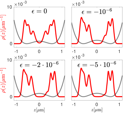
Figure 7: Charge distribution profiles for $N=5$ particles, with different $\epsilon$ values. At $\epsilon=0$ the particle in the middle is represented on both sides of the potential barrier, while by increasing the linear detuning, we see that it slowly shifts to one side, changing the positions for the side particles as well.

IV.2 Charge distribution and polarization

The experimental set-up of Ref. [23] also allows measuring charge distributions. In particular, the collective motion of the electrons has been demonstrated by measuring the difference of the charge density, $\Delta\rho(z,\alpha,\epsilon)$, before and after the tunneling, and comparing the results with theoretical computations for $N=3$ (see Fig. 4 in Ref. [23]).

Although experimentally it is not possible to measure non-invasively $\rho(z)$ at the most interesting point, $\epsilon=0$, we can compute $\rho(z)$ for any value of $\epsilon$, and study its evolution upon changing the bias $\epsilon$. The redistribution of charge as a function of bias, as obtained via ED computations is displayed in Fig. 7 for $N=5$ particles. While for $\epsilon\gg\Delta$ two electrons reside on the right and three on the left, for $\epsilon\approx 0$ the system delocalizes between the ”2+3” and ”3+2” states, as reflected by the deformation of the density profile. While the motion of the central electron is certainly dominant, the profile difference, $\Delta\rho(z)$, presented in Fig. 8, clearly indicates that all charges are displaced in course of the quantum tunneling process.

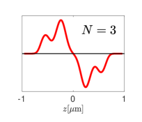
Figure 8: Smeared charge density difference, $\Delta\rho(z)$, between the left and right polarized states for $N=3$ and $N=5$ as a function of the bias, $\epsilon$. The peaks emerging on the sides indicates, that during the tunneling all the three particles change their positions.

We present $\rho(\chi)$ for $N=3$ particles in Fig. 9 for a set of parameters $\alpha$. The classical ground state becomes twofold degenerate at $\alpha=\alpha^{N=3}_{\text{cl}}\approx 4.45$. Quantum fluctuations, however, shift this threshold to $\alpha^{N=3}_{\text{0}}\approx 6.9$, and tunneling takes place only for $\alpha\gtrsim 6.3$. Fig. 9 also displays the charge polarization, Eq. (14). The main contribution to the polarization comes from the tunneling of the central electron, and the rearrangement of electrons on the right and the left yields a much smaller contribution. At $\epsilon\approx 0$, the central electron is strongly delocalized between the two sides, while the lateral electrons gradually shift as the central charge is transferred.

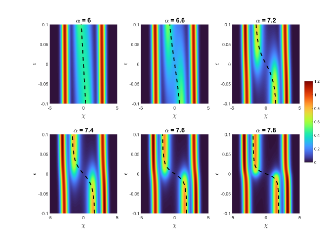
Figure 9: Charge distribution (color code) and the polarization (dashed line) for $N=3$ particles. The classical critical point is at $\alpha_{\text{cl}}^{N=3}\approx 4.45$, but tunneling occurs only above $\alpha^{N=3}_{0}\approx 6.9$. Most of the polarization is carried by the central electron. Quantum fluctuations of lateral electrons facilitate the tunneling process.

This seems to suggest that lateral electrons are merely spectators of the tunneling event. This is, however, not true. As already discussed above, the profile $\Delta\rho$ clearly demonstrates that all electrons participate in the tunneling process. This is corroborated by our instanton computations, which show that lateral electrons participate in collective vibrations and thereby enhance quantum fluctuations, which largely facilitate the quantum-tunneling process, as captured by the increased prefactor $R_{0}$ in Eq. (11).

V Conclusion

In this work, we combined several theoretical approaches to describe the tunneling of a small Wigner crystal confined within a suspended carbon nanotube and subject to a double-well potential, studied experimentally in Ref. [23]. For an odd number of electrons and for sufficiently high barriers, the classical ground state of the crystal becomes degenerate, and the crystal tunnels between these two states.

A combination of instanton theory, Density Matrix Renormalization Group and a peculiar Exact Diagonalization method allowed us to describe the low energy spectrum of the crystal as well as its charge distribution, and determine the amplitude of collective tunneling in this very strongly interacting regime, and compare with the experimental results [23]. The methods above provide us a consistent picture, compare well with the experiments, and provide a quantitative theory for the experimental data in Ref. [23].

Interestingly, the tunneling crossover does not take place at the classical bifurcation point, as naively expected, but due to quantum fluctuations it is shifted towards somewhat higher barrier values (higher values of $\alpha$ in Eq. (7)). Indeed, our calculations clearly demonstrate both the importance of quantum fluctuations and the collective nature of tunneling.

Rather surprisingly, we find that the presence of other particles increases the tunneling amplitude rather than reducing it. Indeed, in typical tunneling problems the presence of environment leads to a suppression of tunneling due to Anderson’s orthogonality catastrophe [44, 45]. The physics behind this latter phenomenon is that the motion of one (test) particle influences the wave function of all other particles, too, which therefore act back and suppress the motion of aforementioned particle. In our case, however, collective quantum fluctuations of the electron chain seem to play a much more important role: they facilitate the motion of the innermost electron, which is mostly responsible for the tunneling.

Quite astonishingly, the experimental data as well as our theoretical curves exhibit a universal scaling collapse. At a first sight, this seems quite natural: one can identify a single collective coordinate within the instanton theory, which moves in an effective double well potential, and is responsible for the tunneling of the crystal. This would support the emergence of a universal tunneling curve – apart from some overall scaling factors. However, the remaining degrees of freedom renormalize the tunneling amplitude for $N\geq 3$ particles by a renormalization factor that has an intrinsic gate voltage dependence. Apparently, the latter renormalization factor, although without an obvious reason, does not spoil the aforementioned universal scaling within our computational accuracy.

Finally, let us briefly commenting on the role of spin and chiral degrees of freedom. Electrons or holes in a nanotube possess chirality and spin quantum numbers. In this work, however, we assumed that the spin sector is completely incoherent, and can therefore be considered as classical. This is certainly justified for the experiments in Ref. [23]. At very low temperatures or smaller interactions, however, exchange processes may become important, and disregarding the spin sector entirely may not be quite appropriate [46, 29]. This is further complicated by the presence of spin-orbit coupling, which couples spin and chiral degrees of freedom, and leads to the freezing out of the charge carriers’ SU(4) spin. The description of the residual SU(2) degrees of freedom [28] and their impact on the tunneling process at low temperatures as well as the role of the SU(4)$\to$SU(2) cross-over is an open and challenging problem, left for future investigation.

Appendix A Computation of the instanton prefactor.

Performing the Gaussian integral in Eq. (10), one finds [26]

$$K(\mathbold{\chi}_{0}^{\prime},\mathbold{\chi}_{0})=\text{e}^{-S_{E}}\sqrt{\frac{2S_{E}}{\pi}}\left[\frac{\det^{\prime}\left(-\partial_{\vartheta}^{2}+V^{\prime\prime}_{0}(\vartheta))\right)}{\det\left(-\partial_{\vartheta}^{2}+\omega^{2}_{\rm{soft}}\right)}\right]^{-1/2}$$ (23)

$$\times\left[\frac{\det^{\prime}\left(-\partial_{\vartheta}^{2}{\bf{1}}+{\bf{\Omega}}^{2}(\vartheta)\right)}{\det\left(-\partial_{\vartheta}^{2}{\bf{1}}+{\bf{\Omega}}^{2}_{0}\right)}\right]^{-1/2}.$$

Here the first line represents the propagator’s classical contribution, whereas the second line denotes the contribution arising from quantum fluctuations.

The softest vibrational mode at the base of the classical trajectory $\bm{\chi}_{cl}(\tau)$ has a frequency $\omega_{\rm{soft}}$, and $\det^{\prime}$ denotes the functional determinant, computed by excluding the zero eigenvalue in the energy spectrum of the tunneling.

The $(N-1)\times(N-1)$ matrix ${\bf{\Omega}}_{0}$ represents the eigenfrequencies around the equilibrium position, $\bm{\chi}_{0}$. The $(N-1)\times(N-1)$ matrix ${\bf{\Omega}}(\vartheta)$ is computed using the vibrational eigenvectors along the instanton trajectory. Technically, to compute the contribution coming from the quantum fluctuations is a delicate issue. We followed the approach introduced in Ref. [26] and introduce the Jacobian fields through $\left(-\partial_{\vartheta}^{2}{\bf{1}}+{\bf{\Omega}}^{2}(\vartheta)\right)\mathbf{J}(\vartheta)=0$ which is related with the derivative of the instanton $\bm{\kappa}(\vartheta)\propto\dot{\bm{\chi}}(\vartheta)$. Introducing a function ${\bf\Xi}(\vartheta)=\dot{\bm{\kappa}}(\vartheta)\,\bm{\kappa}(\vartheta)^{-1}$ that satisfies a differential equation, ${\bf{\dot{\Xi}}}=\varrho/(1-\vartheta^{2})\left({\bf{\Omega}^{2}}(\vartheta)-{\bf{\Xi}}^{2}(\vartheta)\right)$, with the boundary condition that the particles behavior is of a harmonic oscillator, we can express the tunnel splitting in a compact form.

An essential aspect of this calculation is the introduction of a coordinate basis transformation on the $N$ dimensional trajectory. The new basis consists of one parallel and $N-1$ perpendicular unit vectors with respect to the trajectory, as opposed to $N$ coordinates that describe the independent particles. It is found that the trajectory’s direction is parallel to the eigenvector of the softest vibrational eigenmode.

In this description the trajectory and subsequent calculations can be simplified to an arc-length parametrized effectively one-dimensional description. This takes place in the effective potential, that is created by the collective motion of particles as in Fig. 3. This enables us to calculate the quantity $P[{\mathbold{\chi}}_{cl}(s)]$ as a one-dimensional equation. This renormalization constant depends on the momentum-like quantity $p_{0}=\sqrt{2[v_{N}^{\rm{max}}-v_{N}^{\rm{min}}]}$

$$P[{\mathbold{\chi}}_{cl}(s)]=\exp\left\{\int\limits_{-1}^{0}{\rm{d}}\vartheta\,\frac{\varrho}{(1-\vartheta^{2})}\left(\omega_{\rm{soft}}-\frac{\partial p_{0}(s)}{\partial s}\right)\right\}.$$ (24)

This arc-length parametrized picture makes it possible to express $\mathbold{\Omega}$ by the curvature of the trajectory parametrized either by imaginary time or arc-length, although the two descriptions yield the same results. Solving numerically the set of differential equations ${\bf{\dot{\Xi}}}=\varrho/(1-\vartheta^{2})\left({\bf{\Omega}^{2}}(\vartheta)-{\bf{\Xi}}^{2}(\vartheta)\right)$ with the appropriate boundary conditions that states, that indeed for times close to $\vartheta=\pm 1$ the particles behave like a collective harmonic oscillator.

The renormalization factor $R_{0}(\alpha,N)$ then can be expressed as

$$R_{0}(\alpha,N)=\sqrt{\frac{\det{\bf{\Omega}}_{0}}{\det{\bf{\Xi}}(0)}}\times$$

$$\exp\left\{\int\limits_{-1}^{0}{\rm{d}}\vartheta\,\frac{\varrho}{(1-\vartheta^{2})}\,{\rm{Tr}}({\bf{\Omega}}_{0}-{\bf{\Xi}}(\vartheta))\right\}.$$ (25)

References

- Wigner [1934] E. Wigner, On the interaction of electrons in metals, Phys. Rev. 46, 1002 (1934).
- Schulz [1993] H. J. Schulz, Wigner crystal in one dimension, Phys. Rev. Lett. 71, 1864 (1993).
- Andrei et al. [1988] E. Y. Andrei, G. Deville, D. C. Glattli, F. I. B. Williams, E. Paris, and B. Etienne, Observation of a magnetically induced wigner solid, Phys. Rev. Lett. 60, 2765 (1988).
- Jiang et al. [1990] H. W. Jiang, R. L. Willett, H. L. Stormer, D. C. Tsui, L. N. Pfeiffer, and K. W. West, Quantum liquid versus electron solid around =1/5 landau-level filling, Phys. Rev. Lett. 65, 633 (1990).
- Goldman et al. [1990] V. J. Goldman, M. Santos, M. Shayegan, and J. E. Cunningham, Evidence for two-dimentional quantum wigner crystal, Phys. Rev. Lett. 65, 2189 (1990).
- Buhmann et al. [1991] H. Buhmann, W. Joss, K. von Klitzing, I. V. Kukushkin, A. S. Plaut, G. Martinez, K. Ploog, and V. B. Timofeev, Novel magneto-optical behavior in the wigner-solid regime, Phys. Rev. Lett. 66, 926 (1991).
- Santos et al. [1992] M. B. Santos, J. Jo, Y. W. Suen, L. W. Engel, and M. Shayegan, Effect of landau-level mixing on quantum-liquid and solid states of two-dimensional hole systems, Phys. Rev. B 46, 13639 (1992).
- Shirahama and Kono [1995] K. Shirahama and K. Kono, Dynamical transition in the wigner solid on a liquid helium surface, Phys. Rev. Lett. 74, 781 (1995).
- Yoon et al. [1999] J. Yoon, C. C. Li, D. Shahar, D. C. Tsui, and M. Shayegan, Wigner crystallization and metal-insulator transition of two-dimensional holes in gaas at , Phys. Rev. Lett. 82, 1744 (1999).
- Chen et al. [2006] Y. P. Chen, G. Sambandamurthy, Z. H. Wang, R. M. Lewis, L. W. Engel, D. C. Tsui, P. D. Ye, L. N. Pfeiffer, and K. W. West, Melting of a 2d quantum electron solid in high magnetic field, Nature Physics 2, 452 (2006).
- Zhu et al. [2010] H. Zhu, Y. P. Chen, P. Jiang, L. W. Engel, D. C. Tsui, L. N. Pfeiffer, and K. W. West, Observation of a pinning mode in a wigner solid with fractional quantum hall excitations, Phys. Rev. Lett. 105, 126803 (2010).
- Tiemann et al. [2014] L. Tiemann, T. D. Rhone, N. Shibata, and K. Muraki, Nmr profiling of quantum electron solids in high magnetic fields, Nature Physics 10, 648 (2014).
- Deng et al. [2016] H. Deng, Y. Liu, I. Jo, L. N. Pfeiffer, K. W. West, K. W. Baldwin, and M. Shayegan, Commensurability oscillations of composite fermions induced by the periodic potential of a wigner crystal, Phys. Rev. Lett. 117, 096601 (2016).
- Deng et al. [2019] H. Deng, L. N. Pfeiffer, K. W. West, K. W. Baldwin, L. W. Engel, and M. Shayegan, Probing the melting of a two-dimensional quantum wigner crystal via its screening efficiency, Phys. Rev. Lett. 122, 116601 (2019).
- Ma et al. [2020] M. K. Ma, K. A. Villegas Rosales, H. Deng, Y. J. Chung, L. N. Pfeiffer, K. W. West, K. W. Baldwin, R. Winkler, and M. Shayegan, Thermal and quantum melting phase diagrams for a magnetic-field-induced wigner solid, Phys. Rev. Lett. 125, 036601 (2020).
- Regan et al. [2020] E. C. Regan, D. Wang, C. Jin, M. I. Bakti Utama, B. Gao, X. Wei, S. Zhao, W. Zhao, Z. Zhang, K. Yumigeta, M. Blei, J. D. Carlström, K. Watanabe, T. Taniguchi, S. Tongay, M. Crommie, A. Zettl, and F. Wang, Mott and generalized wigner crystal states in wse2/ws2 moirésuperlattices, Nature 579, 359 (2020).
- Smoleński et al. [2021] T. Smoleński, P. E. Dolgirev, C. Kuhlenkamp, A. Popert, Y. Shimazaki, P. Back, X. Lu, M. Kroner, K. Watanabe, T. Taniguchi, I. Esterlis, E. Demler, and A. Imamoğlu, Signatures of wigner crystal of electrons in a monolayer semiconductor, Nature 595, 53 (2021).
- Zhou et al. [2021] Y. Zhou, J. Sung, E. Brutschea, I. Esterlis, Y. Wang, G. Scuri, R. J. Gelly, H. Heo, T. Taniguchi, K. Watanabe, G. Zaránd, M. D. Lukin, P. Kim, E. Demler, and H. Park, Bilayer wigner crystals in a transition metal dichalcogenide heterostructure, Nature 595, 48 (2021).
- Li et al. [2021] H. Li, S. Li, E. C. Regan, D. Wang, W. Zhao, S. Kahn, K. Yumigeta, M. Blei, T. Taniguchi, K. Watanabe, S. Tongay, A. Zettl, M. F. Crommie, and F. Wang, Imaging two-dimensional generalized wigner crystals, Nature 597, 650 (2021).
- Villegas Rosales et al. [2021] K. A. Villegas Rosales, S. K. Singh, M. K. Ma, M. S. Hossain, Y. J. Chung, L. N. Pfeiffer, K. W. West, K. W. Baldwin, and M. Shayegan, Competition between fractional quantum hall liquid and wigner solid at small fillings: Role of layer thickness and landau level mixing, Phys. Rev. Res. 3, 013181 (2021).
- Falson et al. [2022] J. Falson, I. Sodemann, B. Skinner, D. Tabrea, Y. Kozuka, A. Tsukazaki, M. Kawasaki, K. von Klitzing, and J. H. Smet, Competing correlated states around the zero-field wigner crystallization transition of electrons in two dimensions, Nature Materials 21, 311 (2022).
- Hossain et al. [2022] M. S. Hossain, M. K. Ma, K. A. Villegas-Rosales, Y. J. Chung, L. N. Pfeiffer, K. W. West, K. W. Baldwin, and M. Shayegan, Anisotropic two-dimensional disordered wigner solid, Phys. Rev. Lett. 129, 036601 (2022).
- Shapir et al. [2019] I. Shapir, A. Hamo, S. Pecker, C. P. Moca, Ö. Legeza, G. Zarand, and S. Ilani, Imaging the electronic wigner crystal in one dimension, Science 364, 870 (2019).
- Deshpande and Bockrath [2008] V. V. Deshpande and M. Bockrath, The one-dimensional wigner crystal in carbon nanotubes, Nature Physics 4, 314 (2008).
- Secchi and Rontani [2010] A. Secchi and M. Rontani, Wigner molecules in carbon-nanotube quantum dots, Phys. Rev. B 82, 035417 (2010).
- Mil’nikov and Nakamura [2001] G. V. Mil’nikov and H. Nakamura, Practical implementation of the instanton theory for the ground-state tunneling splitting, The Journal of Chemical Physics 115, 6881 (2001).
- Charlier et al. [2007] J.-C. Charlier, X. Blase, and S. Roche, Electronic and transport properties of nanotubes, Rev. Mod. Phys. 79, 677 (2007).
- Sárkány et al. [2017] L. Sárkány, E. Szirmai, C. P. Moca, L. Glazman, and G. Zaránd, Wigner crystal phases in confined carbon nanotubes, Phys. Rev. B 95, 115433 (2017).
- Fiete [2007] G. A. Fiete, Colloquium: The spin-incoherent luttinger liquid, Rev. Mod. Phys. 79, 801 (2007).
- Coleman [1988] S. Coleman, Aspects of Symmetry (Cambridge university press, 1988).
- Ciafaloni and Destri [1988] M. Ciafaloni and C. Destri, Effective potential and asymmetric instantons, Nuovo Cim. A 99, 449 (1988).
- Grafke et al. [2015] T. Grafke, R. Grauer, and T. Schäfer, The instanton method and its numerical implementation in fluid mechanics, Journal of Physics A: Mathematical and Theoretical 48, 333001 (2015).
- Richardson [2018] J. O. Richardson, Ring-polymer instanton theory, International Reviews in Physical Chemistry 37, 171 (2018).
- Vanderbilt and Louie [1984] D. Vanderbilt and S. G. Louie, A monte carlo simulated annealing approach to optimization over continuous variables, Journal of Computational Physics 56, 259 (1984).
- MacKenzie [2000] R. MacKenzie, Path integral methods and applications (2000), arXiv:quant-ph/0004090 [quant-ph] .
- White [1992] S. R. White, Density matrix formulation for quantum renormalization groups, Phys. Rev. Lett. 69, 2863 (1992).
- Schollwöck [2005] U. Schollwöck, The density-matrix renormalization group, Rev. Mod. Phys. 77, 259 (2005).
- Schollwöck [2011] U. Schollwöck, The density-matrix renormalization group in the age of matrix product states, Annals of Physics 326, 96 (2011), january 2011 Special Issue.
- McCulloch [2007] I. P. McCulloch, From density-matrix renormalization group to matrix product states, Journal of Statistical Mechanics: Theory and Experiment 2007, P10014 (2007).
- Legeza and Sólyom [2003] Ö. Legeza and J. Sólyom, Optimizing the density-matrix renormalization group method using quantum information entropy, Phys. Rev. B 68, 195116 (2003).
- Legeza and Fáth [1996] Ö. Legeza and G. Fáth, Accuracy of the density-matrix renormalization-group method, Physical Review B 53, 14349 (1996).
- Hagymási and Legeza [2016] I. Hagymási and O. Legeza, Entanglement, excitations, and correlation effects in narrow zigzag graphene nanoribbons, Phys. Rev. B 94, 165147 (2016).
- Simon [1984] H. D. Simon, Analysis of the symmetric lanczos algorithm with reorthogonalization methods, Linear Algebra and its Applications 61, 101 (1984).
- Anderson [1967] P. W. Anderson, Infrared catastrophe in fermi gases with local scattering potentials, Phys. Rev. Lett. 18, 1049 (1967).
- Leggett et al. [1987] A. J. Leggett, S. Chakravarty, A. T. Dorsey, M. P. A. Fisher, A. Garg, and W. Zwerger, Dynamics of the dissipative two-state system, Rev. Mod. Phys. 59, 1 (1987).
- Fiete and Balents [2004] G. A. Fiete and L. Balents, Green’s function for magnetically incoherent interacting electrons in one dimension, Phys. Rev. Lett. 93, 226401 (2004).