Discrete analogue of the Weil-Petersson volume in double scaled SYK

Abstract

We show that the connected correlators of partition functions in double scaled SYK model can be decomposed into “trumpet” and the discrete analogue of the Weil-Petersson volume, which was defined by Norbury and Scott. We explicitly compute this discrete volume for the first few orders in the genus expansion and confirm that the discrete volume reduces to the Weil-Petersson volume in a certain semi-classical limit.

1 Introduction

The Sachdev-Ye-Kitaev (SYK) model is a very useful toy model for the study of quantum gravity Sachdev1993 ; Kitaev1 ; Kitaev2 ; Polchinski:2016xgd ; Maldacena:2016hyu . At low energy, the SYK model is described by the Schwarzian mode which is holographically dual to the Jackiw-Teitelboim (JT) gravity Jackiw:1984je ; Teitelboim:1983ux . In the seminal paper Saad:2019lba , it was found that JT gravity is equivalent to a random matrix model in the double scaling limit and the higher genus amplitudes of JT gravity are obtained by gluing the Weil-Petersson volume with the so-called trumpet partition functions and integrating over the lengths of the geodesic loops.

One can go beyond the realm of the low energy Schwarzian approximation by taking a certain double scaling limit of the SYK model Cotler:2016fpe ; Berkooz:2018jqr , which we will call DSSYK in this paper. As shown in Berkooz:2018jqr , DSSYK is exactly solvable in the planar limit using the technique of the chord diagram and the transfer matrix. In Lin:2022rbf it is suggested that the chord number state $|n\rangle$ appearing in the transfer matrix formalism can be thought of as a state on the bulk Hilbert space and the bulk geodesic length is replaced by a discrete chord number $n$ in DSSYK. In Okuyama:2023byh , the amplitude of a half-wormhole ending on the end of the world brane was computed and it was found that the length of geodesic loop is also discretized in units of the coupling $\lambda$ of DSSYK.

So far, the non-planar contributions of DSSYK have not been fully explored in the literature before. In this paper, we will study the $1/N$ expansion of the matrix model of DSSYK introduced in Jafferis:2022wez . We focus on the correlator of thermal partition functions of DSSYK and ignore the effect of matter field for simplicity. In this case, DSSYK is described by a hermitian one-matrix model with a certain potential $V(M)$, whose explicit form was obtained in Jafferis:2022wez . We find that $n$-point function of the partition function $Z(\beta)$ at genus-$g$ is expanded as

$$Z_{g,n}(\beta_{1},\cdots,\beta_{n})=\sum_{b_{1},\cdots,b_{n}\in\mathbb{Z}_{+}}N_{g,n}(b_{1},\cdots,b_{n})\prod_{i=1}^{n}b_{i}Z_{\text{trumpet}}(\beta_{i},b_{i}),$$ (1)

where $N_{g,n}$ is a discrete analogue of the volume of moduli space of Riemann surfaces introduced by Norbury and Scott norbury2013polynomials . It turns out that the trumpet partition function $Z_{\text{trumpet}}(\beta,b)$ is given by the modified Bessel function of the first kind, which agrees with the result obtained from the analysis of the end of the world brane Okuyama:2023byh . We explicitly compute the discrete volume $N_{g,n}$ for small $(g,n)$ in the matrix model of DSSYK using the technique of Eynard-Orantin’s topological recursion Eynard:2007kz . We find that the discrete volume $N_{g,n}$ of DSSYK reduces to the Weil-Petersson volume in a certain semi-classical limit.

This paper is organized as follows. In section 2, we review the matrix model description of DSSYK obtained in Jafferis:2022wez . In section 3, we introduce the Joukowsky map and compute the spectral curve of the matrix model of DSSYK in Jafferis:2022wez . In section 4, we review the Eynard-Orantin’s topological recursion and the discrete volume $N_{g,n}$ introduced by Norbury and Scott norbury2013polynomials . We show that the connected correlator of partition functions can be decomposed into the discrete volume and the trumpet. We find that the trumpet partition function is given by the modified Bessel function of the first kind. In section 5, we compute the discrete volumes $N_{g,n}$ for the Gaussian matrix model via the topological recursion and check that they are consistent with the known results of the correlators of Gaussian matrix model. In section 6, we compute the discrete volumes $N_{g,n}$ with small $(g,n)$ for the matrix model of DSSYK and confirm that they reduce to the Weil-Petersson volume in the semi-classical limit. Finally, we conclude in section 7 with some discussion on future problems.

2 Matrix model of DSSYK

We first review the result of DSSYK Berkooz:2018jqr and its matrix model representation Jafferis:2022wez . In this paper, we will consider the one-matrix model associated with the random Hamiltonian of the SYK model and we will ignore the effect of matter operators for simplicity.

SYK model is defined by the Hamiltonian for $N$ Majorana fermions $\psi_{i}~{}(i=1,\cdots,N)$ obeying $\{\psi_{i},\psi_{j}\}=2\delta_{i,j}$ with all-to-all $p$-body interaction

$$H=\mathrm{i}^{p/2}\sum_{1\leq i_{1}<\cdots<i_{p}\leq N}J_{i_{1}\cdots i_{p}}\psi_{i_{1}}\cdots\psi_{i_{p}},$$ (2)

where $J_{i_{1}\cdots i_{p}}$ is a random coupling drawn from the Gaussian distribution with the mean and the variance given by

$$\langle J_{i_{1}\cdots i_{p}}\rangle_{J}=0,\quad\langle J_{i_{1}\cdots i_{p}}^{2}\rangle_{J}=\binom{N}{p}^{-1}.$$ (3)

Here and in what follows, $\langle\cdots\rangle_{J}$ refers to the ensemble average over the random coupling $J_{i_{1}\cdots i_{p}}$.

DSSYK is defined by the scaling limit

$$N,p\to\infty\quad\text{with}\quad\lambda=\frac{2p^{2}}{N}:\text{fixed}.$$ (4)

As shown in Berkooz:2018jqr , the ensemble average of the moment $\operatorname{tr}H^{k}$ reduces to a counting problem of the intersection number of chord diagrams

$$\langle\operatorname{tr}H^{k}\rangle_{J}=\sum_{\text{chord diagrams}}q^{\#(\text{intersections})},$$ (5)

where $q$ is given by

$$q=e^{-\lambda}.$$ (6)

Here, $\operatorname{tr}$ in $\operatorname{tr}H^{k}$ refers to the trace over the Fock space of Majorana fermions. Using the technique of the transfer matrix, the disk amplitude $\langle\operatorname{tr}e^{-\beta H}\rangle_{J}$ of DSSYK is explicitly evaluated as Berkooz:2018jqr

$$\langle\operatorname{tr}e^{-\beta H}\rangle_{J}=\int_{0}^{\pi}\frac{d\theta}{2\pi}(q,e^{\pm 2\mathrm{i}\theta};q)_{\infty}e^{-\beta E(\theta)},$$ (7)

where $E(\theta)$ is given by

$$E(\theta)=-a\cos\theta,\qquad a=\frac{2}{\sqrt{1-q}}.$$ (8)

The $q$-Pochhammer symbol is defined by

$$(a;q)_{\infty}=\prod_{k=0}^{\infty}(1-aq^{k}),$$ (9)

and the measure factor in (7) is a shorthand of

$$(q,e^{\pm 2\mathrm{i}\theta};q)_{\infty} =(q;q)_{\infty}(e^{2\mathrm{i}\theta};q)_{\infty}(e^{-2\mathrm{i}\theta};q)_{\infty}.$$ (10)

As argued in Jafferis:2022wez , one can introduce an $N\times N$ hermitian one-matrix model which reproduces (7) at genus-zero in the $1/N$ expansion. We define the partition function of matrix model by

$$\mathcal{Z}=\int dMe^{-N\operatorname{Tr}V(M)}$$ (11)

and the correlator of $Z(\beta)=\operatorname{Tr}e^{\beta M}$ is written as

$$\Biggl{\langle}\prod_{i=1}^{n}Z(\beta_{i})\Biggr{\rangle} =\frac{1}{\mathcal{Z}}\int dMe^{-N\operatorname{Tr}V(M)}\prod_{i=1}^{n}\operatorname{Tr}e^{\beta_{i}M}.$$ (12)

In what follows, we will assume that $V(M)$ is an even function of $M$

$$V(-M)=V(M),$$ (13)

and the eigenvalues are distributed along the segment $x\in[-a,a]$ on the real $x$-axis in the large $N$ limit, where $x$ denotes the eigenvalue of the random matrix $M$.

As usual, the connected correlator of $Z(\beta)$’s admits the genus expansion in the large $N$ limit

$$\Biggl{\langle}\prod_{i=1}^{n}Z(\beta_{i})\Biggr{\rangle}_{\text{conn}}=\sum_{g=0}^{\infty}N^{2-2g-n}Z_{g,n}(\beta_{1},\cdots,\beta_{n}).$$ (14)

Also, the connected correlator of $\operatorname{tr}e^{-\beta H}$ of DSSYK has a similar large $N$ expansion

$$\left\langle\prod_{i=1}^{n}\operatorname{tr}e^{-\beta_{i}H}\right\rangle_{J}^{\text{conn}}=\sum_{g=0}^{\infty}N^{2-2g-n}Z_{g,n}^{\prime}(\beta_{1},\cdots,\beta_{n}).$$ (15)

As argued in Jafferis:2022wez , the leading order (i.e. genus-zero) contribution for the $n$-point function of DSSYK $Z_{0,n}^{\prime}(\beta_{1},\cdots,\beta_{n})$ in (15) agrees with the matrix model result $Z_{0,n}(\beta_{1},\cdots,\beta_{n})$ in (14) by construction of the matrix model potential in Jafferis:2022wez . In particular, the genus-zero one-point function $Z_{0,1}(\beta)$ of the matrix model is equal to the disk amplitude $\langle\operatorname{tr}e^{-\beta H}\rangle_{J}$ of DSSYK in (7). In terms of the genus-zero eigenvalue density $\rho_{0}(x)$ of the matrix model, the disk amplitude is written as

$$\langle\operatorname{tr}e^{-\beta H}\rangle_{J}=Z_{0,1}(\beta)=\int_{-a}^{a}dx\,\rho_{0}(x)e^{\beta x}.$$ (16)

By identifying $x$ with $-E(\theta)$ in (8)

$$x=-E(\theta)=a\cos\theta,$$ (17)

we can read off $\rho_{0}(x)$ from (7)

$$\rho_{0}(x) =\frac{1}{2\pi\sqrt{a^{2}-x^{2}}}(q,e^{\pm 2\mathrm{i}\theta};q)_{\infty}$$ (18)

$$=\frac{1}{2\pi\sqrt{a^{2}-x^{2}}}\sum_{n\in\mathbb{Z}}(-1)^{n}q^{\frac{1}{2}n^{2}}\bigl{[}q^{\frac{1}{2}n}+q^{-\frac{1}{2}n}\bigr{]}T_{2n}(a^{-1}x),$$

where $T_{n}(\cos\theta)=\cos(n\theta)$ denotes the Chebyshev polynomial of the first kind.

From the relation between the eigenvalue density $\rho_{0}(x)$ and the matrix model potential $V(M)$

$$\frac{1}{2}V^{\prime}(x)=\int_{-a}^{a}dx^{\prime}\frac{\rho_{0}(x^{\prime})}{x-x^{\prime}},\quad(x\in[-a,a]),$$ (19)

we find

$$\frac{1}{2}V^{\prime}(x)=\frac{1}{a}\sum_{n=1}^{\infty}(-1)^{n-1}q^{\frac{1}{2}n^{2}}\bigl{[}q^{\frac{1}{2}n}+q^{-\frac{1}{2}n}\bigr{]}U_{2n-1}(a^{-1}x),$$ (20)

where $U_{n}(\cos\theta)=\frac{\sin(n+1)\theta}{\sin\theta}$ denotes the Chebyshev polynomial of the second kind. After integrating $V^{\prime}(x)$ in (20), the matrix model potential $V(M)$ of DSSYK is found to be Jafferis:2022wez

$$V(x)=\sum_{n=1}^{\infty}\frac{(-1)^{n-1}}{n}q^{\frac{1}{2}n^{2}}\bigl{[}q^{\frac{1}{2}n}+q^{-\frac{1}{2}n}\bigr{]}T_{2n}(a^{-1}x).$$ (21)

Note that in the limit $q\to 0$ the potential becomes Gaussian

$$\lim_{q\to 0}V(x)=T_{2}(x/2)=\frac{1}{2}x^{2}+\text{const}.$$ (22)

In Figure 1 we show the plot of $V(x)$ in (21) for $q=0.1$ and $q=0.9$.

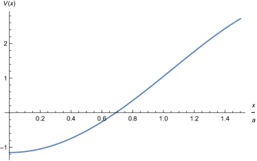
(a) $q=0.1$

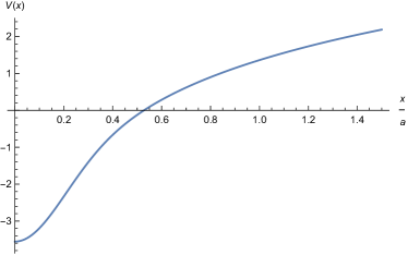
(b) $q=0.9$

Figure 1: Plot of the matrix model potential $V(x)$ in (21) as a function of $x/a$ with $a=\frac{2}{\sqrt{1-q}}$. We show the plot of $V(x)$ for 1(a) $q=0.1$ and 1(b) $q=0.9$.

For general $g\geq 1$, there is no obvious reason to expect the agreement of the matrix model result $Z_{g,n}$ in (14) and the large $N$ expansion of DSSYK $Z^{\prime}_{g,n}$ in (15). Nevertheless, it is tempting to speculate that these two computations actually agree at all genera

$$Z_{g,n}(\beta_{1},\cdots,\beta_{n})=Z_{g,n}^{\prime}(\beta_{1},\cdots,\beta_{n})\quad\forall g\geq 0.$$ (23)

This conjecture (23) is based on a possible holographic dual of DSSYK proposed in Blommaert:2023opb . It is proposed in Blommaert:2023opb that, if we ignore the effect of bulk matter fields, the bulk dual of DSSYK is described as a Poisson-sigma model whose bulk dynamics is topological in nature, in a similar manner as the BF theory description of JT gravity Saad:2019lba . Thus we expect that the path integral of the bulk theory of DSSYK reduces to a computation of a certain volume of the moduli space of Riemann surfaces, which in our case corresponds to the discrete volume $N_{g,n}$. As shown in norbury2013polynomials , $N_{g,n}$ obeys the topological recursion and $N_{g,n}$ at the higher genus $g\geq 1$ is uniquely determined by the genus-zero data $N_{0,n^{\prime}}$. This suggests that the agreement of the matrix model result $Z_{0,n}$ and the DSSYK computation $Z_{0,n}^{\prime}$ at genus-zero implies the agreement $Z_{g,n}=Z^{\prime}_{g,n}$ at higher genus $g\geq 1$ assuming that the bulk dual of DSSYK becomes a topological theory when we ignore the effect of bulk matter fields. Making this argument as a more rigorous proof of (23) is beyond the scope of this paper. In the rest of this paper, we will concentrate on the higher genus computation on the matrix model side (14), which is of interest in its own right regardless of the validity of the conjecture (23).

3 Joukowsky map and spectral curve

When the eigenvalues of random matrix $M$ are distributed along the segment $x\in[-a,a]$, we say that such a matrix model is in the one-cut phase. In this case, the spectral curve of the matrix model is a Riemann surface of genus-zero and the square-root branch-cut can be uniformized by the Joukowsky map (see e.g. Eynard:2008we for a review).

It is well-known that the genus-zero resolvent

$$R(x)=\left\langle\frac{1}{N}\operatorname{Tr}\frac{1}{x-M}\right\rangle_{g=0}$$ (24)

satisfies the loop equation

$$R(x)^{2}=V^{\prime}(x)R(x)-P(x)$$ (25)

with

$$P(x)=\left\langle\frac{1}{N}\operatorname{Tr}\frac{V^{\prime}(x)-V^{\prime}(M)}{x-M}\right\rangle_{g=0}.$$ (26)

The loop equation (25) can be written as a spectral curve for the matrix model

$$y^{2}=\frac{1}{4}V^{\prime}(x)^{2}-P(x),$$ (27)

where $y$ is defined by

$$y=\frac{1}{2}V^{\prime}(x)-R(x).$$ (28)

In the one-cut phase with the support of eigenvalues along the segment $x\in[-a,a]$, $y$ takes the form

$$y=Q(x)\sqrt{x^{2}-a^{2}},$$ (29)

where $Q(x)$ is a regular function of $x$. In other words, $y$ has a square-root branch-point at $x=\pm a$. In this case, the spectral curve (27) can be uniformized by introducing the uniformization parameter $z$

$$x(z)=\frac{a}{2}(z+z^{-1}).$$ (30)

This is known as the Joukowsky map. Then $y$ in (29) becomes

$$y=Q\big{(}x(z)\big{)}\cdot\frac{a}{2}(z-z^{-1}).$$ (31)

One can see that the two branches of the square-root $\sqrt{x^{2}-a^{2}}=\frac{a}{2}(z-z^{-1})$ are exchanged by sending $z$ to its conjugated point $\overline{z}=z^{-1}$

$$z\to\overline{z}=z^{-1}~{}~{}~{}\Rightarrow~{}~{}~{}y\to-y.$$ (32)

Note that $x(z)=x(\overline{z})$ and the cut $[-a,a]$ on the $x$-plane is mapped to the unit circle on the $z$-plane

$$x=a\cos\theta~{}~{}~{}\Rightarrow~{}~{}~{}z=e^{\mathrm{i}\theta}.$$ (33)

In particular, the branch-points $x=\pm a$ correspond to $z=\pm 1$. Also note that the first and the second sheet of the square-root on the $x$-plane correspond to the inside and the outside of the unit circle on the $z$-plane.

The Joukowsky map enables us to solve the genus-zero loop equation (25) by an algebraic means. From (28) and (31), one can show that

$$V^{\prime}\big{(}x(z)\big{)}=R(z)+R(\overline{z}),$$ (34)

where we defined $R(z)=R\big{(}x(z)\big{)}$. This relation has been already appeared in (19). Expanding the left hand side of (34) as

$$V^{\prime}\big{(}x(z)\big{)}=\sum_{k\geq 1}u_{k}(z^{k}+z^{-k})$$ (35)

and using the large $x$ asymptotics of $R(x)\sim 1/x+\mathcal{O}(x^{-2})$, we find

$$R(z)=\sum_{k\geq 1}u_{k}z^{-k}.$$ (36)

Plugging (35) and (36) into (28), $y$ is given by

$$y=\frac{1}{2}\sum_{k\geq 1}u_{k}(z^{k}-z^{-k}).$$ (37)

This $y(z)$ together with $x(z)$ in (30) defines a spectral curve of the hermitian matrix model in the one-cut phase.

3.1 Spectral curve of DSSYK

Let us apply the above formalism to the matrix model of DSSYK. Using the relation

$$U_{2n-1}(w)=2\sum_{j=0}^{n-1}T_{2j+1}(w),$$ (39)

$V^{\prime}(x)$ in (20) becomes

$$V^{\prime}\bigl{(}x(z)\bigr{)}=\frac{2}{a}\sum_{n=1}^{\infty}(-1)^{n-1}q^{\frac{1}{2}n^{2}}\bigl{[}q^{\frac{1}{2}n}+q^{-\frac{1}{2}n}\bigr{]}\sum_{j=0}^{n-1}(z^{2j+1}+z^{-2j-1}).$$ (40)

From (35) and (37), we can read off $y(z)$ for the DSSYK as

$$y(z) =\frac{1}{a}\sum_{n=1}^{\infty}(-1)^{n-1}q^{\frac{1}{2}n^{2}}\bigl{[}q^{\frac{1}{2}n}+q^{-\frac{1}{2}n}\bigr{]}\sum_{j=0}^{n-1}(z^{2j+1}-z^{-2j-1})$$ (41)

$$=\frac{1}{a}\sum_{n=1}^{\infty}(-1)^{n-1}q^{\frac{1}{2}n^{2}}\bigl{[}q^{\frac{1}{2}n}+q^{-\frac{1}{2}n}\bigr{]}\frac{z^{2n}+z^{-2n}-2}{z-z^{-1}}$$

$$=\frac{1}{a}\sum_{n\in\mathbb{Z}}(-1)^{n-1}q^{\frac{1}{2}n(n+1)}\frac{z^{2n}+z^{-2n}-2}{z-z^{-1}}$$

$$=\frac{1}{a}(z-z^{-1})\prod_{n=1}^{\infty}(1-q^{n})(1-z^{2}q^{n})(1-z^{-2}q^{n}).$$

In the last step, we have used the Jacobi triple product identity

$$\sum_{n\in\mathbb{Z}}(-1)^{n-1}q^{\frac{1}{2}n(n+1)}w^{n}=(w^{-1}-1)\prod_{n=1}^{\infty}(1-q^{n})(1-wq^{n})(1-w^{-1}q^{n}).$$ (42)

To summarize, the spectral curve of DSSYK is given by

$$x(z)=\frac{a}{2}(z+z^{-1}),\quad y(z)=\frac{1}{a}(z-z^{-1})\prod_{n=1}^{\infty}(1-q^{n})(1-z^{2}q^{n})(1-z^{-2}q^{n}),$$ (43)

with $a=\frac{2}{\sqrt{1-q}}$. When $q=0$, (43) reduces to the spectral curve of the Gaussian matrix model

$$x(z)=z+z^{-1},\quad y(z)=\frac{1}{2}(z-z^{-1}).$$ (44)

4 Trumpet and volume in the one-matrix model

In this section, we will show that the $n$-point function of partition functions at genus-$g$ is decomposed into the discrete volume $N_{g,n}$ and the trumpet, as shown in (1).

Let us first review the discrete volume $N_{g,n}(b_{1},\cdots,b_{n})$ introduced in norbury2013polynomials in the case of the one-matrix model. To this end, it is convenient to consider the connected correlator of the resolvent $\operatorname{Tr}\frac{1}{x-M}$ instead of $\operatorname{Tr}e^{\beta M}$

$$\left\langle\prod_{i=1}^{n}\operatorname{Tr}\frac{1}{x_{i}-M}\right\rangle_{\text{conn}}=\sum_{g=0}^{\infty}N^{2-2g-n}W_{g,n}(x_{1},\cdots,x_{n}).$$ (45)

It is also useful to introduce $\omega_{g,n}$ by

$$\omega_{g,n}(z_{1},\cdots,z_{n})=W_{g,n}\bigl{(}x(z_{1}),\cdots,x(z_{n})\bigr{)}dx(z_{1})\cdots dx(z_{n}).$$ (46)

For the Joukowsky map $x(z)$ in (30), $dx(z)$ is given by

$$dx(z)=\frac{a}{2}(1-z^{-2})dz.$$ (47)

$\omega_{g,n}$ can be computed by the Eynard-Orantin’s topological recursion Eynard:2007kz ; Eynard:2008we

$$\omega_{g,n+1}(z_{0},J)=\sum_{\alpha=\pm 1}\underset{z=\alpha}{\text{Res}}K(z_{0},z)\Bigl{[}\omega_{g-1,n+2}(z,\overline{z},J)+\sum_{h=0}^{g}\sum^{\prime}_{I\subset J}\omega_{h,1+|I|}(z,I)\omega_{g-h,1+n-|I|}(\overline{z},J\backslash I)\Bigr{]}$$ (48)

with the initial condition

$$\omega_{0,2}(z_{1},z_{2}) =\frac{dz_{1}dz_{2}}{(z_{1}-z_{2})^{2}}.$$ (49)

In (48), the prime in the summation means that $(h,I)=(0,\emptyset),(g,J)$ are excluded and the recursion kernel $K(z_{0},z)$ is given by

$$K(z_{0},z) =-\frac{\int_{z^{\prime}=\overline{z}}^{z}\omega_{0,2}(z_{0},z^{\prime})}{4y(z)dx(z)}=-\frac{z}{2ay(z)(z_{0}-z)(z_{0}-z^{-1})dz}dz_{0}.$$ (50)

Following norbury2013polynomials , we expand $\omega_{g,n}$ as

$$\omega_{g,n}(z_{1},\cdots,z_{n})=\sum_{b_{1},\cdots,b_{n}\in\mathbb{Z}_{+}}N_{g,n}(b_{1},\cdots,b_{n})\prod_{i=1}^{n}b_{i}z_{i}^{b_{i}-1}dz_{i}.$$ (51)

As discussed in norbury2013polynomials , $N_{g,n}(b_{1},\cdots,b_{n})$ is naturally interpreted as a discrete analogue of the volume of the moduli space of Riemann surfaces. In particular, for the Gaussian matrix model $N_{g,n}(b_{1},\cdots,b_{n})$ counts the number of lattice points on the moduli space of curves norbury2008counting .

We can express $Z_{g,n}(\beta_{1},\cdots,\beta_{n})$ defined in (14) in terms of the volume $N_{g,n}(b_{1},\cdots,b_{n})$ and the discrete version of the trumpet introduced in Jafferis:2022wez ; Okuyama:2023byh . Note that $Z_{g,n}$ is written in terms of the genus-$g$ resolvent $W_{g,n}$ as

$$Z_{g,n}(\beta_{1},\cdots,\beta_{n})=\oint\prod_{i=1}^{n}\frac{dx_{i}}{2\pi\mathrm{i}}e^{\beta_{i}x_{i}}W_{g,n}(x_{1},\cdots,x_{n}),$$ (52)

where the contour of integration $\oint dx$ surrounds the cut $[-a,a]$ on the $x$-plane. By the Joukowsky map (30) this contour is mapped to a circle surrounding $z=0$ on the $z$-plane and (52) is rewritten as

$$Z_{g,n}(\beta_{1},\cdots,\beta_{n}) =\prod_{i=1}^{n}\oint_{z_{i}=0}\frac{1}{2\pi\mathrm{i}}e^{\frac{\beta_{i}a}{2}(z_{i}+z_{i}^{-1})}\omega_{g,n}(z_{1},\cdots,z_{n}).$$ (53)

Using the relation

$$e^{\frac{\beta a}{2}(z+z^{-1})}=\sum_{n\in\mathbb{Z}}I_{n}(\beta a)z^{-n},$$ (54)

and (51), the $z_{i}$-integral in (53) is evaluated as

$$Z_{g,n}(\beta_{1},\cdots,\beta_{n}) =\sum_{b_{1},\cdots,b_{n}\in\mathbb{Z}_{+}}N_{g,n}(b_{1},\cdots,b_{n})\prod_{i=1}^{n}b_{i}Z_{\text{trumpet}}(\beta_{i},b_{i}),$$ (55)

where the trumpet partition function is given by

$$Z_{\text{trumpet}}(\beta,b)=I_{b}(\beta a).$$ (56)

Here $I_{\nu}(z)$ denotes the modified Bessel function of the first kind. This result of trumpet (56) agrees with the one obtained from the analysis of end of the world brane in Okuyama:2023byh .

We should stress that the decomposition (55) of $Z_{g,n}$ into the volume $N_{g,n}$ and the trumpet is valid for arbitrary one-matrix models in the one-cut phase. Note also that $Z_{\text{trumpet}}(\beta,b)$ in (56) is universal in the sense that it does not depend on the details of the matrix model potential $V(M)$; it only depends on the endpoint $a$ of the cut.

5 Discrete volume in the Gaussian matrix model

As a warm-up, let us consider the discrete volume $N_{g,n}$ in the Gaussian matrix model. One can easily compute $\omega_{g,n}$ for small $(g,n)$ by solving the topological recursion (48) for the spectral curve of the Gaussian matrix model (44). For instance, $\omega_{0,3}$ is given by

$$\omega_{0,3}(z_{1},z_{2},z_{3}) =\sum_{\alpha=\pm 1}\underset{z=\alpha}{\text{Res}}K(z_{1},z)\bigl{[}\omega_{0,2}(z,z_{2})\omega_{0,2}(\overline{z},z_{3})+\omega_{0,2}(z,z_{3})\omega_{0,2}(\overline{z},z_{2})\bigr{]}$$ (57)

$$=2\frac{(1+z_{1}z_{2}+z_{2}z_{3}+z_{3}z_{1})(z_{1}+z_{2}+z_{3}+z_{1}z_{2}z_{3})}{(1-z_{1}^{2})^{2}(1-z_{1}^{2})^{2}(1-z_{1}^{2})^{2}}dz_{1}dz_{2}dz_{3}.$$

From the definition of $N_{g,n}$ in (51), we can extract $N_{0,3}$ as

$$N_{0,3}(b_{1},b_{2},b_{3})=P_{b_{1}+b_{2}+b_{3}},$$ (58)

where $P_{b}$ denotes the projection to even $b$

$$P_{b}=\frac{1+(-1)^{b}}{2}.$$ (59)

In a similar manner we find

$$N_{1,1}(b) =\frac{b^{2}-4}{48}P_{b},$$ (60)

$$N_{2,1}(b) =\frac{(b^{2}-2^{2})(b^{2}-4^{2})(b^{2}-6^{2})(5b^{2}-32)}{8847360}P_{b},$$

$$N_{1,2}(b_{1},b_{2}) =\frac{(b_{1}^{2}+b_{2}^{2}-2)(b_{1}^{2}+b_{2}^{2}-10)}{384}P_{b_{1}+b_{2}}+\frac{1}{32}P_{b_{1}}P_{b_{2}}.$$

This agrees with the result in norbury2008counting as expected. As discussed in Okuyama:2023byh , for $(g,n)=(0,2)$ it is natural to define

$$N_{0,2}(b_{1},b_{2})=\frac{1}{b_{1}}\delta_{b_{1},b_{2}},$$ (61)

which reproduces the known result of cylinder amplitude in the Gaussian matrix model Akemann:2001st .

It turns out that the sum over $b_{i}$ in (55) can be performed in a closed form. For instance,

$$Z_{1,1}(\beta) =\sum_{b=1}^{\infty}N_{1,1}(b)bI_{b}(2\beta)=\frac{(2\beta)^{2}I_{2}(2\beta)}{48},$$ (62)

$$Z_{2,1}(\beta) =\sum_{b=1}^{\infty}N_{2,1}(b)bI_{b}(2\beta)=\frac{(2\beta)^{4}I_{4}(2\beta)}{1280}+\frac{(2\beta)^{5}I_{5}(2\beta)}{9216},$$

which reproduces the $1/N$ corrections to the $1/2$ BPS Wilson loop in $\mathcal{N}=4$ super Yang-Mills Drukker:2000rr , which is described by the Gaussian matrix model due to the supersymmetric localization Pestun:2007rz . One can also check that the known results of $Z_{g,n}$ of the Gaussian matrix model in Akemann:2001st ; Okuyama:2018aij are reproduced from $N_{g,n}$ in (58) and (60) by summing over $b_{i}$ in (55).

As shown in norbury2008counting , the semi-classical limit of $N_{g,n}$ reproduces the so-called Kontsevich volume

$$\lim_{\lambda\to 0}N_{g,n}(\lambda^{-1}L_{1},\cdots,\lambda^{-1}L_{n})=2^{3-2g-n}\lambda^{-2(3g-3+n)}V^{\text{K}}(L_{1},\cdots,L_{n}),$$ (63)

where the Kontsevich volume is defined by

$$V^{\text{K}}(L_{1},\cdots,L_{n})=\int_{\overline{\mathcal{M}}_{g,n}}\exp\left(\frac{1}{2}\sum_{i=1}^{n}L_{i}^{2}\psi_{i}\right).$$ (64)

In (63) we assumed $\lambda^{-1}L_{i}\in 2\mathbb{Z}_{+}$ and $\psi_{i}$ in (64) is the so-called $\psi$-class on the moduli space $\overline{\mathcal{M}}_{g,n}$ of genus-$g$ Riemann surfaces with $n$ punctures. The power of $\lambda$ on the right hand side of (63) is related to the dimension of $\overline{\mathcal{M}}_{g,n}$

$$\dim\overline{\mathcal{M}}_{g,n}=2(3g-3+n).$$ (65)

6 Discrete volume in DSSYK

Now let us consider the discrete volume $N_{g,n}$ for the matrix model of DSSYK. Using the spectral curve of DSSYK in (43), we can compute $\omega_{g,n}$ by the topological recursion and extract the volume $N_{g,n}$ from the small $z_{i}$ expansion of $\omega_{g,n}$ in (51). In this manner, we find the first few terms of $N_{g,n}$ in the matrix model of DSSYK

$$\widetilde{N}_{0,3}(b_{1},b_{2},b_{3})= P_{b_{1}+b_{2}+b_{3}},$$ (66)

$$\widetilde{N}_{1,1}(b)= \left[\frac{b^{2}-4}{48}+\frac{\zeta_{q}(2)}{2}\right]P_{b},$$

$$\widetilde{N}_{2,1}(b)= \Biggl{[}\frac{(5b^{2}-32)(b^{2}-2^{2})(b^{2}-4^{2})(b^{2}-6^{2})}{8847360}+\frac{(29b^{2}-108)(b^{2}-2^{2})(b^{2}-4^{2})}{92160}\zeta_{q}(2)$$

$$+\frac{(29b^{2}-48)(b^{2}-2^{2})}{1536}\zeta_{q}(4)+\frac{(359b^{2}-624)(b^{2}-2^{2})}{7680}\zeta_{q}(2)^{2}$$

$$+\frac{191b^{2}+4}{96}\zeta_{q}(2)^{3}+\frac{81b^{2}+28}{32}\zeta_{q}(2)\zeta_{q}(4)+\frac{7(5b^{2}+4)}{48}\zeta_{q}(6)$$

$$+\frac{845}{48}\zeta_{q}(2)^{4}+\frac{185}{16}\zeta_{q}(4)^{2}+\frac{399}{8}\zeta_{q}(2)^{2}\zeta_{q}(4)+\frac{203}{6}\zeta_{q}(2)\zeta_{q}(6)+\frac{105}{8}\zeta_{q}(8)\Biggr{]}P_{b},$$

$$\widetilde{N}_{1,2}(b_{1},b_{2})= \Biggl{[}\frac{(b_{1}^{2}+b_{2}^{2}-10)(b_{1}^{2}+b_{2}^{2}-2)}{384}+\frac{b_{1}^{2}+b_{2}^{2}-2}{4}\zeta_{q}(2)+\frac{7\zeta_{q}(2)^{2}}{2}+\frac{5\zeta_{q}(4)}{2}\Biggl{]}P_{b_{1}+b_{2}}$$

$$+\frac{1}{32}P_{b_{1}}P_{b_{2}}.$$

Here we defined

$$\widetilde{N}_{g,n}(b_{1},\cdots,b_{n})=(q;q)_{\infty}^{3(2g-2+n)}N_{g,n}(b_{1},\cdots,b_{n}),$$ (67)

and $\zeta_{q}(s)$ is a $q$-analogue of the zeta function

$$\zeta_{q}(s)=\sum_{n=1}^{\infty}\left(q^{-\frac{1}{2}n}-q^{\frac{1}{2}n}\right)^{-s}.$$ (68)

In the semi-classical limit $\lambda\to 0$, the discrete length $b_{i}\in\mathbb{Z}_{+}$ becomes a continuous geodesic length $L_{i}\in\mathbb{R}_{+}$ and they are related by Okuyama:2023byh

$$L_{i}=\lambda b_{i},$$ (69)

where $\lambda$ is the coupling of DSSYK defined in (4). From our result of $N_{g,n}$ of DSSYK in (66), we observe that $N_{g,n}$ reduces to the Weil-Petersson volume in the semi-classical limit

$$\lim_{\lambda\to 0}N_{g,n}(\lambda^{-1}L_{1},\cdots,\lambda^{-1}L_{n})=2c^{2-2g-n}\lambda^{-2(3g-3+n)}V^{\text{WP}}_{g,n}(L_{1},\cdots,L_{n}).$$ (70)

Here we assumed $\lambda^{-1}L_{i}\in 2\mathbb{Z}_{+}$ and $c$ is given by

$$c=2(q;q)_{\infty}^{3},$$ (71)

and the Weil-Petersson volume is defined by

$$V^{\text{WP}}_{g,n}(L_{1},\cdots,L_{n})=\int_{\overline{\mathcal{M}}_{g,n}}\exp\left(2\pi^{2}\kappa+\frac{1}{2}\sum_{i=1}^{n}L_{i}^{2}\psi_{i}\right),$$ (72)

where $\kappa$ denotes the $\kappa$-class (also known as the first Miller-Morita-Mumford class). For small $(g,n)$ the explicit form of the Weil-Petersson volume reads

$$V^{\text{WP}}_{0,3}(L_{1},L_{2},L_{3}) =1,$$ (73)

$$V^{\text{WP}}_{1,1}(L) =\frac{L^{2}}{48}+\frac{\pi^{2}}{12},$$

$$V^{\text{WP}}_{2,1}(L) =\frac{L^{8}}{442368}+\frac{29\pi^{2}L^{6}}{138240}+\frac{139\pi^{4}L^{4}}{23040}+\frac{169\pi^{6}L^{2}}{2880}+\frac{29\pi^{8}}{192},$$

$$V^{\text{WP}}_{1,2}(L_{1},L_{2}) =\frac{(L_{1}^{2}+L_{2}^{2})^{2}}{192}+\frac{\pi^{2}(L_{1}^{2}+L_{2}^{2})}{12}+\frac{\pi^{4}}{4}.$$

Using the fact that the small $\lambda$ limit of $\zeta_{q}(s)$ with $q=e^{-\lambda}$ reduces to the ordinary zeta function $\zeta(s)$

$$\lim_{\lambda\to 0}\zeta_{q}(s)=\lambda^{-s}\zeta(s),$$ (74)

one can see that the factor of $\pi$ in the Weil-Petersson volume in (73) is correctly reproduced from the semi-classical limit of $N_{g,n}$ in (66).

Since the power of $c$ in (70) is the Euler characteristic $\chi=2-2g-n$ of the genus-$g$ Riemann surface with $n$ punctures, $c$ can be absorbed into the definition of the genus counting parameter. The overall factor of $2$ in (70) comes from the fact that there are two branch-points $z=\pm 1$.

In the semi-classical limit, the sum over $b_{i}$ in (55) becomes the integral over $L_{i}$ and the trumpet in (56) reduces to that of JT gravity. As discussed in Okuyama:2023byh , the semi-classical limit of trumpet is obtained by zooming in on the edge of the spectrum $E(\theta)=-a$. By rescaling $\theta=\lambda k$ and $b=\lambda^{-1}L$, the semi-classical limit of trumpet in (56) becomes

$$I_{b}(\beta a) =\int_{0}^{\pi}\frac{d\theta}{2\pi}e^{\beta a\cos\theta}2\cos(b\theta)$$ (75)

$$\approx\int_{0}^{\infty}\frac{\lambda dk}{\pi}e^{\beta a-\frac{1}{2}\beta a\lambda^{2}k^{2}}\cos(Lk)$$

$$=\lambda e^{\beta a}Z_{\text{trumpet}}(\beta\lambda^{3/2},L)$$

where we defined the continuum version of the trumpet as

$$Z_{\text{trumpet}}(\beta,L)=\int_{0}^{\infty}\frac{dk}{\pi}e^{-\beta k^{2}}\cos(Lk)=\frac{e^{-\frac{L^{2}}{4\beta}}}{\sqrt{4\pi\beta}}.$$ (76)

Then (55) becomes

$$Z_{g,n}(\beta_{1},\cdots,\beta_{n})=\prod_{i=1}^{n}\int_{0}^{\infty}dL_{i}L_{i}Z_{\text{trumpet}}(\beta_{i},L_{i})V^{\text{WP}}_{g,n}(L_{1},\cdots,L_{n}),$$ (77)

up to an overall normalization. This reproduces the result of JT gravity matrix model Saad:2019lba , as expected. Thus, our expression of $Z_{g,n}$ in (55) can be thought of as the DSSYK analogue of the genus expansion of the multi-boundary correlators, where the Weil-Petersson volume $V^{\text{WP}}_{g,n}$ is replaced by the discrete volume $N_{g,n}$.

7 Conclusions and outlook

In this paper, we have studied the matrix model of DSSYK in Jafferis:2022wez by focusing on the correlators involving the Hamiltonian only. Then DSSYK is described by a hermitian one-matrix model with the potential (21). We found the spectral curve (43) of this matrix model and computed the discrete volume $N_{g,n}$ using the technique of Eynard-Orantin’s topological recursion. We have checked that our discrete volume $N_{g,n}$ reduces to the Weil-Petersson volume in the semi-classical limit (70). As shown in (55), the multi-boundary correlator $Z_{g,n}$ of DSSYK can be constructed by gluing the discrete volume $N_{g,n}$ and the trumpets, and summing over the discrete lengths $b_{i}$. We found that the trumpet is given by the modified Bessel function (56) universally for arbitrary one-matrix models in the one-cut phase.

There are several interesting open questions. Although we have checked the relation (70) between the Weil-Petersson volume $V^{\text{WP}}_{g,n}$ and the discrete volume $N_{g,n}$ of DSSYK for small $(g,n)$, we do not have a general proof of (70). It would be interesting find a proof of (70) along the lines of norbury2008counting ; norbury2013polynomials .

We observed that the integral over the geodesic length $L$ in JT gravity is replaced by the sum over the discrete length $b$ if we do not take a double scaling limit of matrix model and consider the ordinary large $N$ ’t Hooft expansion. As we saw in (75), the double scaling limit of matrix model amounts to taking a low energy limit of DSSYK. If we go beyond the realm of low energy approximation and keep the whole spectrum $E(\theta)=-a\cos\theta$ of DSSYK, we start to see a discrete structure of the bulk spacetime which is described by the ordinary large $N$ ’t Hooft expansion of the matrix model. Namely, the bulk spacetime of DSSYK is a discrete random surface generated by the ’t Hooft double-line diagram with polygonal faces tHooft:1973alw ; Brezin:1977sv . This is similar in spirit to the work of Gopakumar and collaborators Gopakumar:2011ev ; Gopakumar:2012ny ; Gopakumar:2022djw on the holography of Gaussian matrix model. In Gopakumar:2011ev ; Gopakumar:2012ny ; Gopakumar:2022djw , it is found that the moduli integral in the ’t Hooft expansion of matrix model receives contributions only from certain discrete points on the moduli space, which is reminiscent of the counting of lattice points on the moduli space of curves to define $N_{g,n}$ in norbury2008counting . It would be interesting to develop a lattice counting interpretation of $N_{g,n}$ for the matrix model of DSSYK as well.

On general grounds, we expect that the $1/N$ expansion of the correlator in (14) is an asymptotic series and it receives a non-perturbative correction of the order $e^{-NA(q)}$ with some instanton action $A(q)$. It would be interesting to study the analogue of ZZ branes in DSSYK via the approach of resurgence as in Eynard:2023qdr .

In this paper, we have ignored the effect of matter field for simplicity. It is argued in Jafferis:2022wez that if we include the matter operators in DSSYK, it is described by a two-matrix model. It would be interesting to study the two-matrix model in Jafferis:2022wez by generalizing our work on the one-matrix sector of DSSYK. We leave this as an interesting future problem.