Abstract

Motivated by LDBC SNB [1, 2], LDBC FinBench (Financial Benchmark) intends to define a benchmark characterized by special data and query patterns in financial industry to test graph database systems to make the evaluation of graph databases representative, reliable and comparable, especially in financial scenarios.

Similar to LDBC SNB [1, 2], LDBC FinBench consists of two workloads that focus on different functionalities: the Transaction workload and the Analytics workload (future work for now). This document contains the definition of workloads including a detailed description of the datasets and queries, and also an explanation about the workflow to use the benchmark.

Inspired by LDBC SNB [1, 2] (LDBC’s Social Network Benchmark), a task force is organized by AntGroup(Ant Group Co., Ltd.) and formed by the principal actors in the field of financial graph-like data management under the guidance and help from LDBC to design LDBC FinBench (LDBC’s Financial Benchmark) which is more applicable to financial scenarios. The task force is committed to define a framework that can fairly test and compare different graph-based technologies where the dataset and workload are carefully designed with the rich practical experience of members in the financial industry by hosting the financial business itself or serving other financial entities. LDBC FinBench is an industrial and academic initiative that is distinguished and characterized by the special features and patterns in the financial industry. In this version, the task force has finished the design of the benchmark framework without the analytics workload which is future work. Meantime, the task force has also organized a developer group to develop the benchmark suite for LDBC FinBench. The benchmark suite is currently under development according to the benchmark framework design. In the future, LDBC FinBench will be improved continuously with more feedback and more workloads including analytics workload will be designed and added. Please feel free to contact us if you have some suggestions, or if you are interested in joining in LDBC FinBench. This document contains:

• A detailed specification of the data and workloads in the whole LDBC FinBench.

• A detailed specification of the workflow and instructions about how to use the benchmark suite.

• A detailed specification of the auditing rules and the full disclosure report’s required contents.

Definitions

DataGen:

The data generator provided by the LDBC FinBench, which is responsible for generating the data needed to run the benchmark.

DBMS:

A DataBase Management System.

LDBC FinBench:

Linked Data Benchmark Council Financial Benchmark.

Query Mix:

Refers to the ratio between read and update queries of a workload, and the frequency at which they are issued.

SF (Scale Factor):

The LDBC FinBench is designed to target systems of different sizes and scales. The scale factor determines the size of the data used to run the benchmark, measured in Gigabytes.

SUT:

The System Under Test is defined to be the database system where the benchmark is executed.

Test Driver:

A program provided by the LDBC FinBench, which is responsible for executing the different workloads and gathering the results.

Full Disclosure Report (FDR):

The FDR is a document that allows the reproduction of any benchmark result by a third-party. This contains a complete description of the SUT and the circumstances of the benchmark run, the configuration of SUT, dataset and test driver,

Test Sponsor:

The Test Sponsor is the company officially submitting the Result with the FDR and will be charged the filing fee. Although multiple companies may sponsor a Result together, for the purposes of the LDBC processes the Test Sponsor must be a single company. A Test Sponsor need not be a LDBC member. The Test Sponsor is responsible for maintaining the FDR with any necessary updates or corrections. The Test Sponsor is also the name used to identify the Result.

Workload:

A workload refers to a set of queries of a given nature (interactive, analytical, business), how they are issued and at which rate.

Chapter 1 Introduction

1.1 Motivation

Inspired by LDBC SNB [1, 2], a task force proposed by AntGroup [3] is formed by the principal actors in the field of financial graph-like data management with help from LDBC to design a new benchmark, LDBC FinBench (LDBC’s Financial Benchmark). The task force intends to define a framework that is more applicable to financial scenarios to fairly test and compare different graph-based technologies. To this end, they carefully design the dataset and workload using their rich practical experience as members of the financial industry. LDBC FinBench is distinguished and characterized by the special features and patterns in the financial industry.

1.2 Relevance to the Industry

LDBC FinBench is intended to provide the following value to these relevant stakeholders:

• For users facing graph processing tasks in the financial industry, LDBC FinBench provides a recognizable scenario against which it is possible to compare the merits of different products and technologies. By covering a wide variety of scales and price points, LDBC FinBench can serve as an aid to technology selection.

• For vendors of graph database technology, LDBC FinBench provides a checklist of features and performance characteristics that helps in product positioning and can serve to guide new development.

• For researchers, both industrial and academic, the LDBC FinBench dataset and workload provide interesting challenges in multiple choke point areas, and help compare the efficiency of existing technology in these areas.

The technological scope of LDBC FinBench comprises all systems that one might conceivably use to perform financial data management tasks including Graph database management systems (Neo4j, TuGraph, Galaxybase, etc.), Graph processing frameworks (Giraph, Ligra, etc.), RDF database systems (Virtuoso, AWS Neptune, etc.), Relational database systems (MySQL, Oracle, etc.), NoSQL database systems (key-value stores such as HBase, Redis, MongoDB, CouchDB, or even MapReduce systems like Hadoop and Pig).

1.3 Participation of Industry and Academia

Initially, the LDBC FinBench task force is formed by relevant actors mainly from industry. In the process of design and development, we also received supports and suggestions from fellows in academia. All the participants have contributed with their experience and expertise to make this benchmark a credible effort. The list of participants is as follows.

• AntGroup (entity)

• CreateLink (entity)

• Ultipa (entity)

• StarGraph (entity)

• Vesoft (entity)

• Pometry (entity)

• Katana (entity)

• Intel (entity)

• TigerGraph (entity)

• Koji Annoura (individual)

1.4 Software Components

The source code of this specification and the benchmark suite is available open-source:

• LDBC FinBench Specification: https://github.com/ldbc/ldbc_finbench_docs

• LDBC FinBench Data Generator: https://github.com/ldbc/ldbc_finbench_DataGen

• LDBC FinBench Driver: https://github.com/ldbc/ldbc_finbench_driver

• Transaction Workload Implementation: https://github.com/ldbc/ldbc_finbench_transaction_impls

• Analytics Workload: future work

Note that the main branch for these repositories is under development by default. Please refer to the releases and branch started with v and named vX.X.X for stable versions.

1.5 Related Projects

Along with LDBC FinBench, LDBC [4] provides other benchmarks as well:

• LDBC SNB [1, 2] measures the performance of all systems relevant to linked data operating a social network.

• The Semantic Publishing Benchmark (SPB) [5] measures the performance of semantic databases operating on RDF datasets.

• The Graphalytics benchmark [6] measures the performance of graph analysis operations (PageRank, local clustering coefficient).

Chapter 2 Benchmark Overview

2.1 Practice basis

The task force members design LDBC FinBench with their rich practical experience in financial industry based on a comprehensive survey of financial scenarios including Risk Control, AML (Anti-Money Laundering), KYC (Know Your Customer), Stock Recommendation and so on.

2.2 Design Concepts

LDBC FinBench is intended to be a credible, fair and representative benchmark. It’s designed with the following concepts:

• Based on real systems. The task force members gathering together from industry and academia intend to design LDBC FinBench to express and emphasize the special patterns of data and workload distinguished from other popular benchmarks. To do that, LDBC FinBench is designed based on the rich practical experience of members and additional surveys.

• Comprehensive and complete. LDBC FinBench is intended to cover most demands encountered in the management of complexly structured data in financial scenarios.

• Challenging and instructive. Benchmarks are known to direct product development in certain directions. LDBC FinBench is informed by state-of-the-art in database research and industry practice to offer optimization challenges.

• Easy to use and extendable. As a benchmark offering value to many relevant stakeholders, LDBC FinBench is designed to be easy to use. The effort for obtaining test results with it should be small.

• Modularized. LDBC FinBench is broken into parts both in design and benchmark suite that can be individually addressed to stimulate innovation without imposing an overly high threshold for participation.

• Reproducible and documented. LDBC FinBench is intended to specify the auditing rules and provide full disclosure reports of auditing of benchmark runs in accordance with the LDBC Bylaws [7].

2.3 New features in FinBench

LDBC SNB [1, 2], one of the earlier LDBC benchmarks, is modeled around the operation of a real social network site. It defines a data schema that represents a realistic social network including people and their activities during a period of time and also the workloads mimic the different usage scenarios found in operating a real social network site. Compared with LDBC SNB [1, 2], LDBC FinBench is characterized by the special features and patterns of the data schema and queries that represent the characteristics of financial scenarios.

2.3.1 Data Schema

The data schema for LDBC FinBench is designed to reflect the real data in the financial systems. Frequent financial entities in real systems include accounts, medium, persons, companies, loans, etc. The entities are vertices in the data schema while the edges reflect financial activities, fund transferred from one account to another. In their data schema, financial scenarios have these distinguished characteristics compared to regular social networks.

• Multiple edges can exist between two vertices, Many transfer records exist between two accounts

• Dynamic attribute exists in vertex to mark entities status, an account is marked as blocked

• Quantity attribute exists in edge, Transfer edge has quantity attribute amount

The designed data schema is specified in Chapter 3.

2.3.2 Workloads

In workloads and queries, financial scenarios have these distinguished characteristics.

• More tight latency, some queries need to return in less than 100ms.

• Write operations updating attributes, marking an account as blocked.

• Recursive Path Filtering. Some queries filter data with backward dependency in variable-length paths, finding all transfer paths A-[${e_{1}}$]->..-[${e_{k}}$]->B where the timestamp of each transfer edge ${e_{i}}$ in the path is larger than that of the previous ${e_{i-1}}$. In this pattern, the variable length path is qualified by the edge quantity attributes or the aggregation in the path, either along one path or a set of paths.

• Read-write Query, which is a query sequence with a mix of reads and writes reflecting the complexity of financial systems. Read-write query describes a desired pattern that risk control policies are checked, and corresponding actions are taken before financial activities like transfers are written down to storage. See Section 4.3 for details.

• Truncation. In financial scenarios, the degree of hub vertex may reach million and even billion scales, especially when traversing on a graph. To handle the discordance between the tight latency requirements and power-law distribution of data in the system, truncation is introduced to reduce the complexity of queries. See Section 4.2 for details.

In LDBC FinBench, there are two kinds of workloads:

• Transaction Workload. It includes queries with a tight latency bound, which are usually queries hopping a few steps from a start vertice. There are complex reads, simple reads, write operations, and read-write queries in transaction workload. The Transaction Workload is specified in Chapter 5.

• Analytics Workload. It is supposed to include more complicated queries, triggers and pre-computed values in online systems. This part is future work that will be designed and discussed in the following versions. The Analytics Workload is specified in Chapter 6.

2.4 Benchmark Workflow

See Chapter 8 for the execution workflow of LDBC FinBench.

Chapter 3 Data Definition

This chapter describes the dataset used by LDBC FinBench, including the data schema design and the data generation process. Generally, we design LDBC FinBench balancing reality and abstraction. There are some annotations about the compromises in data design,

• Although multiple persons/companies may own the same account in reality, in the schema, an account is owned by only a single person or company for simplicity.

• Although rejected transactions may be recorded to support future loan decisions, only approved transactions/transfers are recorded in the benchmark dataset.

• Considering the number of daily active users (DAU) of financial systems in reality, there will be many signIn edges between medium and account vertices. However, we do not generate so many signIn edges aligning to reality with a limit in the simulation of the data generation process since systems usually circumvent the problem by adding a medium attribute to edges like transfer and withdraw to record the medium users used.

3.1 Data Types

Table 3.1 describes the different data types used in the benchmark. Compared with LDBC SNB [1, 2], there is a new compound type, Path, which is widely applied in financial scenarios reflecting traces, fund transfer traces.

Type	Description
ID	Integer type with 64-bit precision. All IDs within a single entity type (Person) are unique, but different entity types (a Person and an Account) might have the same ID.
32-bit Integer	Integer type with 32-bit precision
64-bit Integer	Integer type with 64-bit precision
32-bit Float	Floating type with 32-bit precision
64-bit Float	Floating type with 64-bit precision
String	Variable length text of size 40 Unicode characters
Long String	Variable length text of size 256 Unicode characters
Text	Variable length text of size 2000 Unicode characters
Date	Date with a precision of a day, encoded as a string with the following format: yyyy-mm-dd, where yyyy is a four-digit integer representing the year, the year, mm is a two-digit integer representing the month and dd is a two-digit integer representing the day.
DateTime	Date with a precision of milliseconds, encoded as a string with the following format: yyyy-mm-ddTHH:MM:ss.sss+0000, where yyyy is a four-digit integer representing the year, the year, mm is a two-digit integer representing the month and dd is a two-digit integer representing the day, HH is a two-digit integer representing the hour, MM is a two-digit integer representing the minute and ss.sss is a five-digit fixed point real number representing the seconds up to millisecond precision. Finally, the +0000 of the end represents the timezone, which in this case is always GMT.
Boolean	A logical type taking the value of either True of False.
Enum	Enumeration type
Path	A compound type representing a trace which is expressed in an ordered sequence of vertices’ IDs in the trace. For example, [1,3,4,8] expresses a trace 1->3->4->8.

Table 3.1: Description of the data types.

3.1.1 Enumerations

TRUNCATION_ORDER:

The enumeration describes the sort order before truncation. TIMESTAMP_ASCENDING means truncation on ascending order of timestamp.

3.2 Data Schema

Figure 3.1 shows the data schema in UML. The schema defines the structure of the data used in the benchmark in terms of entities and their relations. The data represents a snapshot of the activity in several financial scenarios during a period of time. The schema specifies different entities, their attributes, and their relations. All of them are described in the following sections.

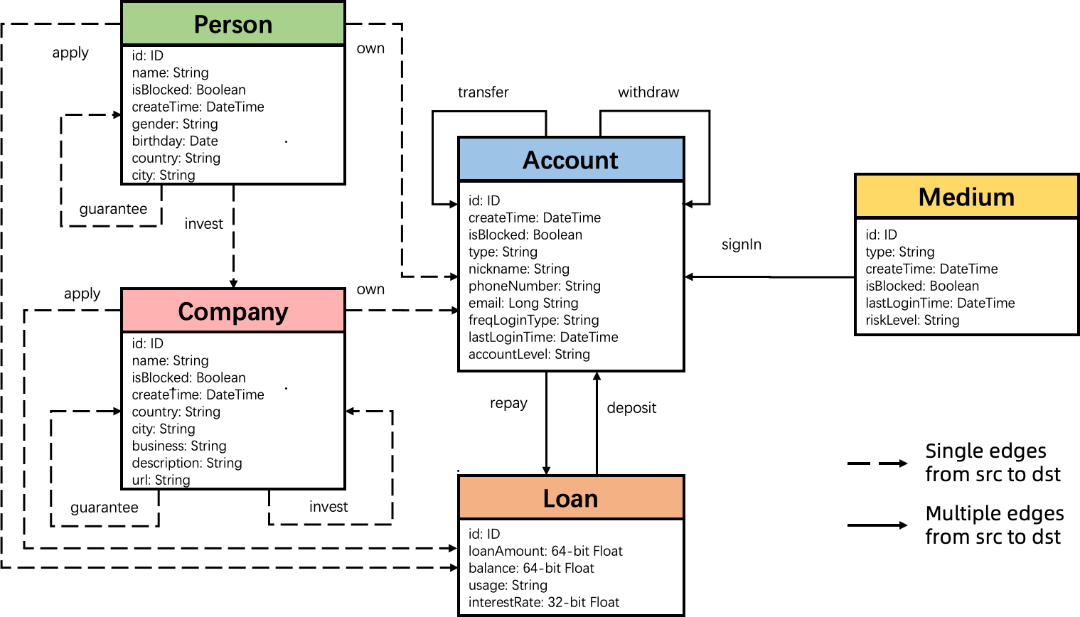
Figure 3.1: The LDBC FinBench data schema

3.2.1 Entities

Person:

A person of the real world. Table 3.2 shows the attributes.

Attribute	Type	Description
id	ID	The identifier of the person.
name	String	The name of the person.
isBlocked	Boolean	If the person is blocked or concerned in systems.
createTime	DateTime	The time when the person created.
gender	String	Gender of the person
birthday	Date	Birthday of the person
country	String	Country of the person
city	String	City of the person

Table 3.2: Attributes of Person entity.

Company:

A company of the real world, which persons or other companies invest in. Table 3.3 shows the attributes.

Attribute	Type	Description
id	ID	The identifier of the company.
name	String	The name of the company.
isBlocked	Boolean	If the company is blocked or concerned in systems.
createTime	DateTime	The time when the company is created.
country	String	Country of the company
city	String	City of the company
business	String	The main business of the company
description	Long String	The description of the company
url	String	The url of the company’s official site

Table 3.3: Attributes of Company entity.

Account:

An account in real-world financial systems, which is registered and owned by persons and companies. It includes many types such as personalDeposit, personalCredit, etc. It can deal with other accounts. Table 3.4 shows the attributes.

Attribute	Type	Description
id	ID	The identifier of the account.
createTime	DateTime	The time when the account is created.
isBlocked	Boolean	If the account is blocked or concerned in systems.
type	String	The type of the account.
nickname	String	The nickname of the account.
phoneNumber	String	The phone number of the account.
email	String	The email of the account.
freqLoginType	String	The frequent login type of the account.
lastLoginTime	DateTime	The last login time of the account.
accountLevel	String	The level of the account.

Table 3.4: Attributes of Account entity.

Loan:

A loan for persons and companies to apply in real world. Table 3.5 shows the attributes.

Attribute	Type	Description
id	ID	The identifier of the loan.
loanAmount	64-bit Float	The amount of a loan.
balance	64-bit Float	The balance of a loan.
usage	String	The usage of a loan.
interestRate	32-bit Float	The interest rate of a loan.

Table 3.5: Attributes of Loan entity.

Medium:

An abstract standing for things that users use to sign in account in the real world, such as IP address, MAC address, phone numbers. Table 3.6 shows the attributes.

Attribute	Type	Description
id	ID	The identifier of the medium.
type	String	The medium type, POS, IP.
createTime	DateTime	The time when the medium is created.
isBlocked	Boolean	If the medium is blocked or concerned in systems.
lastLoginTime	DateTime	The last login time of the medium.
riskLevel	String	The risk level of the medium.

Table 3.6: Attributes of Medium entity.

3.2.2 Relations

Relations connect entities of different types showed in LABEL:table:relations. Except that own has no attributes, the attributes of other relations are shown in the following tables. Note that the Cardinality means the cardinal relationship from the tail to the head of the edge type and the Multiplicity means how many edges exist from the same tail to the same head. For example, the 1 : N cardinality of own means an account can only be owned by a person or a company.

Table 3.7: Description of the data relations.

Name	Tail	Cardinality	Head	Multiplicity	Description
signIn	Medium	N:N	Account	N	An account signed in with a media.
own	Person/ Company	1:N	Account	1	An account owned by a person or a company.
transfer	Account	N:N	Account	N	Fund transferred between two accounts.
withdraw	Account	N:N	Account	N	Fund transferred from an account to another account of type card.
apply	Person/ Company	1:N	Loan	1	A person or a company applies a Loan.
deposit	Loan	N:N	Account	N	Loan fund deposited to an account.
repay	Account	N:N	Loan	N	Loan repaid from an account.
invest	Person/ Company	N:N	Company	1	A person or a company invests into a company.
guarantee	Person/ Company	N:N	Person/ Company	1	A person or a company guarantees another for some reason like loans.

transfer:

Fund transfers between accounts. Table 3.8 shows the attributes.

Attribute	Type	Description
timestamp	DateTime	The time when transfer issues.
amount	64-bit Float	The amount of the transfer.
ordernumber	String	The order number of the transfer.
comment	String	The comment of the transfer.
payType	String	The pay type of the transfer.
goodsType	String	The goods type of the transfer.

Table 3.8: Attributes of transfer relation.

withdraw:

Fund is transferred from one account to another of type card. Table 3.9 shows the attributes.

Attribute	Type	Description
timestamp	DateTime	The time when withdraw issues.
amount	64-bit Float	The amount of the withdraw.

Table 3.9: Attributes of withdraw relation.

repay:

Loan is repaid from an account. Table 3.10 shows the attributes.

Attribute	Type	Description
timestamp	DateTime	The time when repay issues.
amount	64-bit Float	The amount of the repay.

Table 3.10: Attributes of repay relation.

deposit:

Loan fund is deposited to an account. Table 3.11 shows the attributes.

Attribute	Type	Description
timestamp	DateTime	The time when deposit issues.
amount	64-bit Float	The amount of the deposit.

Table 3.11: Attributes of deposit relation.

signIn:

An account is signed in with a Media. Table 3.12 shows the attributes.

Attribute	Type	Description
timestamp	DateTime	The time when signIn happens.
location	String	The location of the signIn.

Table 3.12: Attributes of signIn relation.

invest:

A person or a company invests in a company. Table 3.13 shows the attributes.

Attribute	Type	Description
timestamp	DateTime	The time when the investment happens.
ratio	32-bit Float	The ratio of the investment.

Table 3.13: Attributes of invest relation.

apply:

A person or a company applies for a Loan. Table 3.14 shows the attributes.

Attribute	Type	Description
timestamp	DateTime	The time when apply happens.
organization	String	The organization for the loan.

Table 3.14: Attributes of apply relation.

guarantee:

A person or a company guarantees another for some reason like Loans. Table 3.16 shows the attributes.

Attribute	Type	Description
timestamp	DateTime	The time when guarantee happens.
relationship	String	The relationship between guarantor and applier.

Table 3.15: Attributes of guarantee relation.

own:

A person or a company owns an account. This relation has no attributes.

Attribute	Type	Description
timestamp	DateTime	The time when guarantee happens.

Table 3.16: Attributes of guarantee relation.

3.3 Data Generation

The data generation process is designed to produce a dataset that is as close as possible to the real-world data. The data generator stimulates real-world financial activities in systems and generates the data according to the data schema. See the data generator for more details at https://github.com/ldbc/ldbc_finbench_DataGen.

3.4 Output Data

3.4.1 Data Precision

The datasets are designed and created closely resembling real-world scenarios. DataGen produces financial data having the precision as follows:

• The generated 64-bit Float numbers will have precision up to two decimal places for both the amount and balance values.

• The timestamps are generated with millisecond precision.

3.4.2 Scale Factors

LDBC FinBench defines a set of scale factors (SFs), targeting systems of different sizes and budgets. Namely, the SF1 dataset is 1 GiB, the SF10 is 10 GiB. In the initial version, CSV serializer is provided. We use the default settings to split the data into an initial (bulk-loaded) dataset and incremental data, 97% for initial data and 3% for incremental data. The currently available SFs are the following: 0.01, 0.1, 0.3, 1, 3, 10. By default, all SFs are defined over three years, starting from 2020, and SFs are computed by scaling the number of Persons and Companies in the network. Please refer to Appendix B for the metrics of datasets of different scales.

Chapter 4 Workloads

4.1 Query Annotations

This section describes how to read the query cards in the following sections.

4.1.1 Query Description Format

Queries are described in natural language using a well-defined structure that consists of three sections: description, a concise textual description of the query, parameters, a list of input parameters and their types; results, a list of expected results and their types. Additionally, queries returning multiple results specify sorting criteria and a limit (to return top-$k$ results).

We use the following notation:

• Vertex type: vertice type in the dataset. One word, possibly constructed by appending multiple words together, starting with an uppercase character and following the camel case notation, TagClass represents an entity of type “TagClass”.

• Edge type: edge type in the dataset. One word, possibly constructed by appending multiple words together, starting with a lowercase character and following the camel case notation workAt represents an edge of type “workAt”.

• Attribute: attribute of a vertice or an edge in the dataset. One word, possibly constructed by appending multiple words together, starting with a lowercase character and following the camel case notation, and prefixed by a “.” to dereference the vertice/edge, person.firstName refers to “firstName” attribute on the “person” entity, and studyAt.classYear refers to “classYear” attribute on the “studyAt” edge.

• Unordered Set: an unordered collection of distinct elements. Surrounded by { and } braces, with the element type between them, {String} refers to a set of strings.

• Ordered List: an ordered collection where duplicate elements are allowed. Surrounded by [ and ] braces, with the element type between them, [String] refers to a list of strings.

• Ordered Tuple: a fixed-length, fixed-order list of elements, where elements at each position of the tuple have predefined, possibly different, types. Surrounded by < and > braces, with the element types between them in a specific order <String, Boolean> refers to a 2-tuple containing a string value in the first element and a boolean value in the second, and [<String, Boolean>] is an ordered list of those 2-tuples.

Categorization of results.

Results are categorized according to their source of origin:

• Raw (R), if the result attribute is returned with an unmodified value and type.

• Calculated (C), if the result is calculated from attributes using arithmetic operators, functions, boolean conditions, etc.

• Aggregated (A), if the result is an aggregated value, a count or a sum of another value. If a result is both calculated and aggregated (count(x) + count(y) or avg(x + y)), it is considered an aggregated result.

• Meta (M), if the result is based on type information, the type of a vertice.

4.1.2 Returned Values

Return values are subject to the following rules:

• Path type. The Path type is a sequence of vertices and edges. The Path type is returned as a sequence of vertex and edge identifiers ignoring the multiple edges between the same src and dst vertex.

• Precision of results. In order to maintain consistency of the benchmark results, all floating-point results are rounded to 3 decimal places using standard rounding rules (i.e., round half up).

4.1.3 Other Annotations

To express the patterns better, the pattern diagrams are drawn from the perspective of data rather than the matching pattern in the graph. Here are some annotations to each query card in this section.

• Each row in the result cell represents an attribute to be returned.

• The second column means the data type of returned attribute. If the type is surrounded by , it means that the result is a set, means a string set is returned.

• For each row in the result cell, the third column annotates the category of type of result attribute returned, including R short for Raw, A short for Aggregated, C short for Calculated, S short for Structural. Among them, structural type means types such as while raw type means basic types in contrast.

• In the pattern of each query, the gray dashed box encapsulates the results to return. And the black solid arrows represent the multiple edges from src to dst while the black dashed arrows represent the single edges from src to dst.

4.2 Truncation on Hub Vertices

The high degree of hub vertex is a common feature not only in financial scenarios but also in other scenarios, which is an inevitable challenge that systems face. To solve the problem, systems can either improve the performance to satisfy the computation or just reduce the complexity to meet the latency requirements.

The mechanism is to do truncation on the edges when traversing out from the current vertex, which complies with the discordance. Truncating less-important edges is a useful and practical mechanism to handle the discordance between the tight latency requirements and hub vertices in the system, where the degree of hub vertex may reach a million and even billion scales, especially when traversing the graph. To maintain the consistency of the results, a sort order has to be specified when truncating. Since in financial graphs, users prefer newer data in business. It is reasonable that attribute, timestamp, in the edges is used as the sort order in truncation. With the sort order, truncation is namely a deterministic sampling in traversing.

In the following queries, some parameters are added to describe the behavior of truncation reducing the complexity including the TRUNCATION_LIMIT and TRUNCATION_ORDER. TRUNCATION_ORDER can be TIMESTAMP_ASCENDING, TIMESTAMP_DESCENDING, AMOUNT_ASCENDING, AMOUNT_DESCENDING. At most time, TRUNCATION_ORDER is set to TIMESTAMP_DESCENDING by default.

4.3 Read Write Query

In financial scenarios, risk control is a kind of hot and significant application. Such applications usually detect a specific pattern in the form of linked data before new records like transfers are written to systems. Read-write query, which can also be seen as transaction-wrapped strategies, fits these applications very well since users do not need to worry about translating the patterns to prevent malicious records. A read-write query is composed of read queries and write queries in the previous sections. In most cases, whether to commit the write query depends on the detection result of the read queries. In the initial version, just 3 read-write queries are presented.

Chapter 5 Transaction Workload

This workload consists of a set of relatively simple read queries, write queries and read-write operations that touch a significant amount of data. These queries and operations are usually considered online data processing and analysis in online financial systems. The LDBC FinBench transaction workload consists of four query types:

• Complex-read queries. See Section 5.1. This section contains many basic read queries that are typical in financial scenarios.

• Simple-read queries. See Section 5.2. This section contains many basic read queries that are typical in financial scenarios.

• Write queries. See Section 5.3. This section contains many basic write queries that are typical in financial scenarios.

• Read-write queries. See Section 5.4. This section contains many read-write operations composed of basic reads and writes.

5.1 Complex Read Queries

Transaction / complex-read / 1

query	Transaction / complex-read / 1
title	Blocked medium related accounts
pattern
desc.	Given an Account and a specified time window between startTime and endTime, find all the Account that is signed in by a blocked Medium and has fund transferred via edge1 by at most 3 steps. Note that all timestamps in the transfer trace must be in ascending order(only greater than). Return the id of the account, the distance from the account to given one, the id and type of the related medium. Note: The returned accounts may exist in different distance from the given one.
params	$\mathsf{1}$ id ID id of the start Account $\mathsf{2}$ startTime DateTime begin of the time window $\mathsf{3}$ endTime DateTime end of the time window $\mathsf{4}$ truncationLimit 32-bit Integer maximum edges traversed at each step $\mathsf{5}$ truncationOrder Enum the sort order before truncation at each step
result	$\mathsf{1}$ otherId ID R the id of the account $\mathsf{2}$ accountDistance 32-bit Integer C the distance from the account to the given one $\mathsf{3}$ mediumId ID R the id of medium related to the account $\mathsf{4}$ mediumType String R the type of medium related to the account
sort	$\mathsf{1}$ accountDistance $\uparrow$ $\mathsf{2}$ otherId $\uparrow$ $\mathsf{3}$ mediumId $\uparrow$
CPs	3.2, 3.4, 6.2, 7.1, 7.4, 8.7, 8.8

Transaction / complex-read / 2

query	Transaction / complex-read / 2
title	Fund gathered from the accounts applying loans
pattern
desc.	Given a Person and a specified time window between startTime and endTime, find an Account owned by the Person which has fund transferred from other Accounts by at most 3 steps (edge2) which has fund deposited from a loan. The timestamps of in transfer trace (edge2) must be in ascending order(only greater than) from the upstream to downstream. Return the sum of distinct loan amount, the sum of distinct loan balance and the count of distinct loans.
params	$\mathsf{1}$ id ID id of the start Person $\mathsf{2}$ startTime DateTime begin of the time window $\mathsf{3}$ endTime DateTime end of the time window $\mathsf{4}$ truncationLimit 32-bit Integer maximum edges traversed at each step $\mathsf{5}$ truncationOrder Enum the sort order before truncation at each step
result	$\mathsf{1}$ otherId ID R id of the account related to loan $\mathsf{2}$ sumLoanAmount 64-bit Float A sum of all loans’ amount of the account (rounded to 3 decimal places) $\mathsf{3}$ sumLoanBalance 64-bit Float A sum of all loans’ balance of the account (rounded to 3 decimal places)
sort	$\mathsf{1}$ sumLoanAmount $\downarrow$ $\mathsf{2}$ otherId $\uparrow$
CPs	3.2, 3.4, 6.2, 7.1, 7.4, 8.7, 8.8

Transaction / complex-read / 3

query	Transaction / complex-read / 3
title	Shortest transfer path
pattern
desc.	Given two accounts and a specified time window between startTime and endTime, find the length of shortest path between these two accounts by the transfer relationships. Note that all the edges in the path should be in the time window and of type transfer. Return 1 if src and dst are directly connected. Return -1 if there is no path found.
params	$\mathsf{1}$ id1 ID id of src Account $\mathsf{2}$ id2 ID id of dst Account $\mathsf{3}$ startTime DateTime begin of the time window $\mathsf{4}$ endTime DateTime end of the time window
result	$\mathsf{1}$ shortestPathLength 64-bit Integer C the length of shortest path
CPs	3.2, 3.4, 6.2, 8.7

Transaction / complex-read / 4

query	Transaction / complex-read / 4
title	Three accounts in a transfer cycle
pattern
desc.	Given two accounts src and dst, and a specified time window between startTime and endTime, (1) check whether src transferred money to dst in the given time window (edge1). If edge1 does not exist, return with empty results (the result size is 0). (2) find all other accounts (other1, …, otherN) which received money from dst (edge2) and transferred money to src (edge3) in a specific time. For each of these other accounts, return the id of the account, the sum and max of the transfer amount (edge2 and edge3).
params	$\mathsf{1}$ id1 ID id of the src Account $\mathsf{2}$ id2 ID id of the dst Account $\mathsf{3}$ startTime DateTime begin of the time window $\mathsf{4}$ endTime DateTime end of the time window
result	$\mathsf{1}$ otherId ID R the id of the other account $\mathsf{2}$ numEdge2 64-bit Integer A transfers’ count from otherAccount to srcAccount $\mathsf{3}$ sumEdge2Amount 64-bit Float A sum of transfers from otherAccount to srcAccount (rounded to 3 decimal places) $\mathsf{4}$ maxEdge2Amount 64-bit Float A max of transfers from otherAccount to srcAccount (rounded to 3 decimal places) $\mathsf{5}$ numEdge3 64-bit Integer A transfers’ count from dstAccount to otherAccount $\mathsf{6}$ sumEdge3Amount 64-bit Float A sum of transfers from dstAccount to otherAccount (rounded to 3 decimal places) $\mathsf{7}$ maxEdge3Amount 64-bit Float A max of transfers from dstAccount to otherAccount (rounded to 3 decimal places)
sort	$\mathsf{1}$ sumEdge2Amount $\downarrow$ $\mathsf{2}$ sumEdge3Amount $\downarrow$ $\mathsf{3}$ otherId $\uparrow$
CPs	3.2, 3.4, 6.2, 8.7

Transaction / complex-read / 5

query	Transaction / complex-read / 5
title	Exact Account Transfer Trace
pattern
desc.	Given a Person and a specified time window between startTime and endTime, find the transfer trace from the account (src) owned by the Person to another account (dst) by at most 3 steps. Note that the trace (edge2) must be ascending order(only greater than) of their timestamps. Return all the transfer traces. Note: Multiple edges of from the same src to the same dst should be seen as identical path. And the resulting paths shall not include recurring accounts (cycles in the trace are not allowed). The results may not be in a deterministic order since they are only sorted by the length of the path. Driver will validate the results after sorting.
params	$\mathsf{1}$ id ID id of the start Person $\mathsf{2}$ startTime DateTime begin of the time window $\mathsf{3}$ endTime DateTime end of the time window $\mathsf{4}$ truncationLimit 32-bit Integer maximum edges traversed at each step $\mathsf{5}$ truncationOrder Enum the sort order before truncation at each step
result	$\mathsf{1}$ path Path S a transfer trace. See the requirements in Section 4.1.2
sort	$\mathsf{1}$ pathLength $\downarrow$
CPs	1.1, 3.2, 3.4, 6.2, 7.1, 7.4, 8.7, 8.8

Transaction / complex-read / 6

query	Transaction / complex-read / 6
title	Withdrawal after Many-to-One transfer
pattern
desc.	Given an account of type card and a specified time window between startTime and endTime, find all the connected accounts (mid) via withdrawal (edge2) satisfying, (1) More than 3 transfer-ins (edge1) from other accounts (src) whose amount exceeds threshold1. (2) The amount of withdrawal (edge2) from mid to dstCard whose exceeds threshold2. Return the sum of transfer amount from src to mid, the amount from mid to dstCard grouped by mid.
params	$\mathsf{1}$ id ID id of the card account $\mathsf{2}$ threshold1 64-bit Float threshold of transfer amount $\mathsf{3}$ threshold2 64-bit Float threshold of transfer amount $\mathsf{4}$ startTime DateTime begin of the time window $\mathsf{5}$ endTime DateTime end of the time window $\mathsf{6}$ truncationLimit 32-bit Integer maximum edges traversed at each step $\mathsf{7}$ truncationOrder Enum the sort order before truncation at each step
result	$\mathsf{1}$ midId ID R the id of the middle account $\mathsf{2}$ sumEdge1Amount 64-bit Float A the amount of transfer from src accounts to mid (rounded to 3 decimal places) $\mathsf{3}$ sumEdge2Amount 64-bit Float A the amount of withdrawal from mid to dstCard (rounded to 3 decimal places)
sort	$\mathsf{1}$ sumEdge2Amount $\downarrow$ $\mathsf{2}$ midId $\uparrow$
CPs	3.2, 3.4, 6.2, 8.7

Transaction / complex-read / 7

query	Transaction / complex-read / 7
title	Transfer in/out ratio
pattern
desc.	Given an Account and a specified time window between startTime and endTime, find all the transfer-in (edge1) and transfer-out (edge2) whose amount exceeds threshold. Return the count of src and dst accounts and the ratio of transfer-in amount over transfer-out amount. The fast-in and fash-out means a tight window between startTime and endTime. Return the ratio as -1 if there is no edge2.
params	$\mathsf{1}$ id ID id of mid account $\mathsf{2}$ threshold 64-bit Float transfer amount threshold $\mathsf{3}$ startTime DateTime begin of the time window $\mathsf{4}$ endTime DateTime end of the time window $\mathsf{5}$ truncationLimit 32-bit Integer maximum edges traversed at each step $\mathsf{6}$ truncationOrder Enum the sort order before truncation at each step
result	$\mathsf{1}$ numSrc 32-bit Integer A num of the distinct src accounts $\mathsf{2}$ numDst 32-bit Integer A num of the distinct dst accounts $\mathsf{3}$ inOutRatio 32-bit Float C the amount ratio of transfers-in over transfers-out (rounded to 3 decimal places)
CPs	1.2, 3.2, 3.4, 6.2, 8.7

Transaction / complex-read / 8

query	Transaction / complex-read / 8
title	Transfer trace after loan applied
pattern
desc.	Given a Loan and a specified time window between startTime and endTime, trace the fund transfer or withdraw by at most 3 steps from the account the Loan deposits. Note that the transfer paths of edge1, edge2, edge3 and edge4 are in a specific time range between startTime and endTime. Amount of each transfers or withdrawals between the account and the upstream account should exceed a specified threshold of the upstream transfer. Return all the accounts’ id in the downstream of loan with the final ratio and distanceFromLoan. Note: Upstream of an edge refers to the aggregated total amounts of all transfer-in edges of its source Account.
params	$\mathsf{1}$ id ID id of the Loan $\mathsf{2}$ threshold 32-bit Float threshold of the amount over the upstream’s $\mathsf{3}$ startTime DateTime begin of the time window $\mathsf{4}$ endTime DateTime end of the time window $\mathsf{5}$ truncationLimit 32-bit Integer maximum edges traversed at each step $\mathsf{6}$ truncationOrder Enum the sort order before truncation at each step
result	$\mathsf{1}$ dstId ID R the id of the account in transfer traces $\mathsf{2}$ ratio 32-bit Float C the final ratio of the inflow’s amount of each account over the loan (rounded to 3 decimal places) $\mathsf{3}$ minDistanceFromLoan 32-bit Integer C the min distance from the account to the loan
sort	$\mathsf{1}$ distanceFromLoan $\downarrow$ $\mathsf{2}$ ratio $\downarrow$ $\mathsf{3}$ dstId $\uparrow$
CPs	3.2, 3.4, 6.2, 7.1, 8.7

Transaction / complex-read / 9

query	Transaction / complex-read / 9
title	Money laundering with loan involved
pattern
desc.	Given an account, a bound of transfer amount and a specified time window between startTime and endTime, find the deposit and repay edge between the account and a loan, the transfers-in and transfers-out. Return ratioRepay (sum of all the edge1 over sum of all the edge2), ratioDeposit (sum of edge1 over sum of edge4), ratioTransfer (sum of edge3 over sum of edge4). Return -1 for ratioRepay if there is no edge2 found. Return -1 for ratioDeposit and ratioTransfer if there is no edge4 found. Note: There may be multiple loans that the given account is related to.
params	$\mathsf{1}$ id ID id of the Account $\mathsf{2}$ threshold 64-bit Float threshold of amount $\mathsf{3}$ startTime DateTime begin of the time window $\mathsf{4}$ endTime DateTime end of the time window $\mathsf{5}$ truncationLimit 32-bit Integer maximum edges traversed at each step $\mathsf{6}$ truncationOrder Enum the sort order before truncation at each step
result	$\mathsf{1}$ ratioRepay 32-bit Float C sumEdge1Amount/sumEdge2Amount (rounded to 3 decimal places) $\mathsf{2}$ ratioDeposit 32-bit Float C sumEdge1Amount/sumEdge4Amount (rounded to 3 decimal places) $\mathsf{3}$ ratioTransfer 32-bit Float C sumEdge3Amount/sumEdge4Amount (rounded to 3 decimal places)
CPs	3.2, 3.4, 6.2, 8.7

Transaction / complex-read / 10

query	Transaction / complex-read / 10
title	Similarity of investor relationship
pattern
desc.	Given two Persons and a specified time window between startTime and endTime, find all the Companies the two Persons invest in. Return the Jaccard similarity between the two companies set. Return 0 if there is no edges found connecting to any of these two persons.
params	$\mathsf{1}$ pid1 ID id of Person1 $\mathsf{2}$ pid2 ID id of Person2 $\mathsf{3}$ startTime DateTime begin of the time window $\mathsf{4}$ endTime DateTime end of the time window
result	$\mathsf{1}$ jaccardSimilarity 32-bit Float C Jaccard similarity between two sets (rounded to 3 decimal places)
CPs	3.2, 3.4, 6.2, 8.7

Transaction / complex-read / 11

query	Transaction / complex-read / 11
title	Guarantee Chain Detection
pattern
desc.	Given a Person and a specified time window between startTime and endTime, find all the persons in the guarantee chain until end and their loans applied. Return the sum of loan amount and the count of distinct loans.
params	$\mathsf{1}$ id ID id of the Person $\mathsf{2}$ startTime DateTime begin of the time window $\mathsf{3}$ endTime DateTime end of the time window $\mathsf{4}$ truncationLimit 32-bit Integer maximum edges traversed at each step $\mathsf{5}$ truncationOrder Enum the sort order before truncation at each step
result	$\mathsf{1}$ sumLoanAmount 64-bit Float A sum of the loans’ amount (rounded to 3 decimal places) $\mathsf{2}$ numLoans 32-bit Integer A num of the loans
CPs	3.2, 3.4, 6.2, 7.4, 8.7

Transaction / complex-read / 12

query	Transaction / complex-read / 12
title	Transfer to company amount statistics
pattern
desc.	Given a Person and a specified time window between startTime and endTime, find all the company accounts that s/he has transferred to. Return the ids of the companies’ accounts and the sum of their transfer amount.
params	$\mathsf{1}$ id ID id of the person $\mathsf{2}$ startTime DateTime begin of the time window $\mathsf{3}$ endTime DateTime end of the time window $\mathsf{4}$ truncationLimit 32-bit Integer maximum edges traversed at each step $\mathsf{5}$ truncationOrder Enum the sort order before truncation at each step
result	$\mathsf{1}$ compAccountId ID R the id of the company account $\mathsf{2}$ sumEdge2Amount 64-bit Float A the amount sum transferred to company’s account (rounded to 3 decimal places)
sort	$\mathsf{1}$ sumEdge2Amount $\downarrow$ $\mathsf{2}$ compAccountId $\uparrow$
CPs	3.2, 3.4, 6.2, 7.1, 8.7

5.2 Simple Read Queries

Transaction / simple-read / 1

query	Transaction / simple-read / 1
title	Exact account query
pattern
desc.	Given an id of an Account, find the properties of the specific Account.
params	$\mathsf{1}$ id ID id of the Account
result	$\mathsf{1}$ createTime DateTime R the time when the account created $\mathsf{2}$ isBlocked Boolean R if the account is blocked $\mathsf{3}$ type String R the account type

Transaction / simple-read / 2

query	Transaction / simple-read / 2
title	Transfer-ins and transfer-outs
pattern
desc.	Given an account, find the sum and max of fund amount in transfer-ins and transfer-outs between them in a specific time range between startTime and endTime. Return the sum and max of amount. For edge1 and edge2, return -1 for the max (maxEdge1Amount and maxEdge2Amount) if there is no transfer.
params	$\mathsf{1}$ id ID id of the account $\mathsf{2}$ startTime DateTime begin of the time window $\mathsf{3}$ endTime DateTime end of the time window
result	$\mathsf{1}$ sumEdge1Amount 64-bit Float A sum of transfer-outs (rounded to 3 decimal places) $\mathsf{2}$ maxEdge1Amount 64-bit Float A max of transfer-outs (rounded to 3 decimal places) $\mathsf{3}$ numEdge1 64-bit Integer A count of transfer-outs $\mathsf{4}$ sumEdge2Amount 64-bit Float A sum of transfer-ins (rounded to 3 decimal places) $\mathsf{5}$ maxEdge2Amount 64-bit Float A max of transfer-ins (rounded to 3 decimal places) $\mathsf{6}$ numEdge2 64-bit Integer A count of transfer-outs

Transaction / simple-read / 3

query	Transaction / simple-read / 3
title	Many-to-one blocked account monitoring
pattern
desc.	Given an Account, find the ratio of transfer-ins from blocked Accounts in all its transfer-ins in a specific time range between startTime and endTime. Return the ratio. Return -1 if there is no transfer-ins to the given account.
params	$\mathsf{1}$ id ID id of the dstAccount $\mathsf{2}$ threshold 64-bit Float threshold of transfer amount $\mathsf{3}$ startTime DateTime begin of the time window $\mathsf{4}$ endTime DateTime end of the time window
result	$\mathsf{1}$ blockRatio 32-bit Float A count(edge1) over count(edge2) (rounded to 3 decimal places)

Transaction / simple-read / 4

query	Transaction / simple-read / 4
title	Account transfer-outs over threshold
pattern
desc.	Given an account (src), find all the transfer-outs (edge) from the src to a dst where the amount exceeds threshold in a specific time range between startTime and endTime. Return the count of transfer-outs and the amount sum.
params	$\mathsf{1}$ id ID id of the dstAccount $\mathsf{2}$ threshold 64-bit Float threshold of transfer amount $\mathsf{3}$ startTime DateTime begin of the time window $\mathsf{4}$ endTime DateTime end of the time window
result	$\mathsf{1}$ dstId ID R the id of the dst account $\mathsf{2}$ numEdges 32-bit Integer A num of the transfers from src to dst $\mathsf{3}$ sumAmount 64-bit Float A sum of the transfers from src to dst (rounded to 3 decimal places)
sort	$\mathsf{1}$ sumAmount $\downarrow$ $\mathsf{2}$ dstId $\uparrow$

Transaction / simple-read / 5

query	Transaction / simple-read / 5
title	Account transfer-ins over threshold
pattern
desc.	Given an account (dst), find all the transfer-ins (edge) from the src to a dst where the amount exceeds threshold in a specific time range between startTime and endTime. Return the count of transfer-ins and the amount sum.
params	$\mathsf{1}$ id ID id of the Account $\mathsf{2}$ threshold 64-bit Float threshold of transfer amount $\mathsf{3}$ startTime DateTime begin of the time window $\mathsf{4}$ endTime DateTime end of the time window
result	$\mathsf{1}$ srcId ID R the id of the src account $\mathsf{2}$ numEdges 32-bit Integer A num of the transfers from src to dst $\mathsf{3}$ sumAmount 64-bit Float A sum of the transfers from src to dst (rounded to 3 decimal places)
sort	$\mathsf{1}$ sumAmount $\downarrow$ $\mathsf{2}$ srcId $\uparrow$

Transaction / simple-read / 6

query	Transaction / simple-read / 6
title	Accounts with the same transfer sources of exact account
pattern
desc.	Given an Account (account), find all the blocked Accounts (dstAccounts) that connect to a common account (midAccount) with the given Account (account). Return all the accounts’ id.
params	$\mathsf{1}$ id ID id of the Account $\mathsf{2}$ startTime DateTime begin of the time window $\mathsf{3}$ endTime DateTime end of the time window
result	$\mathsf{1}$ dstId ID R ids of the accounts having same upstream account as the given account
sort	$\mathsf{1}$ dstId $\uparrow$

5.3 Write Queries

In write queries, there are mainly two types of queries, inserts and deletes. In real systems, there are deletion operations besides delete operations. Deletion operations limit the architecture that can be used by a system. On the other hand, systems are supposed to provide API for users to express delete operations no matter with high-level structured languages like GQL and openCypher or low-level storage layer API.

Transaction / write / 1

query	Transaction / write / 1
title	Add a Person
pattern
desc.	Add a Person.
params	$\mathsf{1}$ $personId ID $\mathsf{2}$ $personName String $\mathsf{3}$ $isBlocked Boolean

Transaction / write / 2

query	Transaction / write / 2
title	Add a Company
pattern
desc.	Add a Company.
params	$\mathsf{1}$ $companyId ID $\mathsf{2}$ $companyName String $\mathsf{3}$ $isBlocked Boolean

Transaction / write / 3

query	Transaction / write / 3
title	Add a Medium
pattern
desc.	Add a Medium.
params	$\mathsf{1}$ $mediumId ID $\mathsf{2}$ $mediumType String $\mathsf{3}$ $isBlocked Boolean

Transaction / write / 4

query	Transaction / write / 4
title	Add an Account owned by Person
pattern
desc.	Add an Account and an own edge from Person to the Account.
params	$\mathsf{1}$ $personId ID $\mathsf{2}$ $accountId ID $\mathsf{3}$ $time DateTime $\mathsf{4}$ $accountBlocked Boolean $\mathsf{5}$ $accountType String

Transaction / write / 5

query	Transaction / write / 5
title	Add an Account owned by Company
pattern
desc.	Add an Account and an own edge from Company to the Account.
params	$\mathsf{1}$ $companyId ID $\mathsf{2}$ $accountId ID $\mathsf{3}$ $time DateTime $\mathsf{4}$ $accountBlocked Boolean $\mathsf{5}$ $accountType String

Transaction / write / 6

query	Transaction / write / 6
title	Add Loan applied by Person
pattern
desc.	Add a Loan and add an apply edge from Person to Loan.
params	$\mathsf{1}$ $personId ID $\mathsf{2}$ $loanId ID $\mathsf{3}$ $loanAmount 64-bit Float $\mathsf{4}$ $balance 64-bit Float $\mathsf{5}$ $time DateTime

Transaction / write / 7

query	Transaction / write / 7
title	Add Loan applied by Company
pattern
desc.	Add a Loan and add an apply edge from Company to Loan.
params	$\mathsf{1}$ $companyId ID $\mathsf{2}$ $loanId ID $\mathsf{3}$ $loanAmount 64-bit Float $\mathsf{4}$ $balance 64-bit Float $\mathsf{5}$ $time DateTime

Transaction / write / 8

query	Transaction / write / 8
title	Add invest between Person and Company
pattern
desc.	Add an invest edge from a Person to a Company.
params	$\mathsf{1}$ $personId ID $\mathsf{2}$ $companyId ID $\mathsf{3}$ $time DateTime $\mathsf{4}$ $ratio 64-bit Float

Transaction / write / 9

query	Transaction / write / 9
title	Add invest between Company and Company
pattern
desc.	Add an invest edge from a Company to a Company.
params	$\mathsf{1}$ $companyId1 ID $\mathsf{2}$ $companyId2 ID $\mathsf{3}$ $time DateTime $\mathsf{4}$ $ratio 64-bit Float

Transaction / write / 10

query	Transaction / write / 10
title	Add guarantee between Persons
pattern
desc.	Add a guarantee edge from a Person to another Person.
params	$\mathsf{1}$ $personId1 ID $\mathsf{2}$ $personId2 ID $\mathsf{3}$ $time DateTime

Transaction / write / 11

query	Transaction / write / 11
title	Add guarantee between Companies
pattern
desc.	Add a guarantee edge from a Company to another Company.
params	$\mathsf{1}$ $companyId1 ID $\mathsf{2}$ $companyId2 ID $\mathsf{3}$ $time DateTime

Transaction / write / 12

query	Transaction / write / 12
title	Add transfer between Accounts
pattern
desc.	Add a transfer edge from an Account to another Account.
params	$\mathsf{1}$ $accountId1 ID $\mathsf{2}$ $accountId2 ID $\mathsf{3}$ $time DateTime $\mathsf{4}$ $amount 64-bit Float

Transaction / write / 13

query	Transaction / write / 13
title	Add withdraw between Accounts
pattern
desc.	Add a withdraw edge from an Account to another Account.
params	$\mathsf{1}$ $accountId1 ID $\mathsf{2}$ $accountId2 ID $\mathsf{3}$ $time DateTime $\mathsf{4}$ $amount 64-bit Float

Transaction / write / 14

query	Transaction / write / 14
title	Add repay between Account and Loan
pattern
desc.	Add a repay edge from an Account to a Loan.
params	$\mathsf{1}$ $accountId ID $\mathsf{2}$ $loanId ID $\mathsf{3}$ $time DateTime $\mathsf{4}$ $amount 64-bit Float

Transaction / write / 15

query	Transaction / write / 15
title	Add deposit between Loan and Account
pattern
desc.	Add a deposit edge from a Loan to an Account.
params	$\mathsf{1}$ $loanId ID $\mathsf{2}$ $accountId ID $\mathsf{3}$ $time DateTime $\mathsf{4}$ $amount 64-bit Float

Transaction / write / 16

query	Transaction / write / 16
title	Account signed in with Medium
pattern
desc.	Add a signIn edge from medium to an Account.
params	$\mathsf{1}$ $mediumId ID $\mathsf{2}$ $accountId ID $\mathsf{3}$ $time DateTime

Transaction / write / 17

query	Transaction / write / 17
title	Remove an Account
pattern
desc.	Given an id, remove the Account, and remove the related edges including own, transfer, withdraw, repay, deposit, signIn. Remove the connected Loan vertex in cascade.
params	$\mathsf{1}$ $accountId ID

Transaction / write / 18

query	Transaction / write / 18
title	Block a Account of high risk
pattern
desc.	Set an Account’s isBlocked to True.
params	$\mathsf{1}$ $accountId ID

Transaction / write / 19

query	Transaction / write / 19
title	Block a Person of high risk
pattern
desc.	Set a Person’s isBlocked to True.
params	$\mathsf{1}$ $personId ID

5.4 Read-Write Queries

Transaction / read-write / 1

query	Transaction / read-write / 1
title	Transfer under transfer cycle detection strategy
pattern
compose.	This read-write query contains the reads and writes below, • Transaction / Simple Read / 1 • Transaction / Write / 12 • Transaction / Complex Read / 4 • Transaction / Write / 18
desc.	The workflow of this read write query contains at least one transaction. It works as: • In the very beginning, read the blocked status of related accounts with given ids of two src and dst accounts. The transaction aborts if one of them is blocked. Move to the next step if none is blocked. • Add a transfer edge from src to dst inside a transaction. Given a specified time window between startTime and endTime, find the other accounts which received money from dst and transferred money to src in a specific time. Transaction aborts if a new transfer cycle is formed, otherwise the transaction commits. • If the last transaction aborts, mark the src and dst accounts as blocked in another transaction.
params	$\mathsf{1}$ srcId ID id of the src Account $\mathsf{2}$ dstId ID id of the dst Account $\mathsf{3}$ time DateTime the timestamp of the transfer $\mathsf{4}$ amount 64-bit Float the amount of the transfer $\mathsf{5}$ startTime DateTime begin of the time window $\mathsf{6}$ endTime DateTime end of the time window

Transaction / read-write / 2

query	Transaction / read-write / 2
title	Transfer under in/out ratio strategy
pattern
compose.	This read-write query contains the reads and writes below, • Transaction / Simple Read / 1 • Transaction / Write / 12 • Transaction / Complex Read / 7 • Transaction / Write / 18
desc.	The workflow of this read write query contains at least one transaction. It works as: • In the very beginning, read the blocked status of related accounts with given ids of two src and dst accounts. The transaction aborts if one of them is blocked. Move to the next step if none is blocked. • Add a transfer edge from src to dst inside a transaction. Given a specified time window between startTime and endTime, find all the transfer-in and transfer-out whose amount exceeds amountThreshold. Transaction aborts if the ratio of transfers-in/transfers-out amount exceeds a given ratioThreshold, both for the src and dst account. Otherwise the transaction commits. • If the last transaction aborts, mark the src and dst accounts as blocked in another transaction.
params	$\mathsf{1}$ srcId ID id of the src Account $\mathsf{2}$ dstId ID id of the dst Account $\mathsf{3}$ time DateTime the timestamp of the transfer $\mathsf{4}$ amount 64-bit Float the amount of the transfer $\mathsf{5}$ amountThreshold 64-bit Float transfer amount threshold $\mathsf{6}$ startTime DateTime begin of the time window $\mathsf{7}$ endTime DateTime end of the time window $\mathsf{8}$ ratioThreshold 32-bit Float ratio threshold of transfers-in over transfers-out $\mathsf{9}$ truncationLimit 32-bit Integer maximum edges traversed at each step $\mathsf{10}$ truncationOrder Enum the sort order before truncation at each step

Transaction / read-write / 3

query	Transaction / read-write / 3
title	Guarantee under guarantee chain detection strategy
pattern
compose.	This read-write query contains the reads and writes below, • Transaction / Simple Read / 1 • Transaction / Write / 10 • Transaction / Complex Read / 11 • Transaction / Write / 19
desc.	The workflow of this read write query contains at least one transaction. It works as: • In the very beginning, read the blocked status of related persons with given ids of two src and dst persons. The transaction aborts if one of them is blocked. Move to the next step if none is blocked. • Add a guarantee edge between the src and dst persons inside a transaction. Given a specified time window between startTime and endTime, find all the persons in the guarantee chain of until end and their loans applied. Detect if a guarantee chain pattern formed, only for the src person. Calculate if the amount sum of the related loans in the chain exceeds a given threshold. Transaction aborts if the sum exceeds the threshold. Otherwise the transaction commits. • If the last transaction aborts, mark the src and dst persons as blocked in another transaction.
params	$\mathsf{1}$ srcId ID id of the src Person $\mathsf{2}$ dstId ID id of the dst Person $\mathsf{3}$ time DateTime the timestamp of the guarantee $\mathsf{4}$ threshold 64-bit Float loan amount threshold in the guarantee chain $\mathsf{5}$ startTime DateTime begin of the time window $\mathsf{6}$ endTime DateTime end of the time window $\mathsf{7}$ truncationLimit 32-bit Integer maximum edges traversed at each step $\mathsf{8}$ truncationOrder Enum the sort order before truncation at each step

Chapter 6 Analytics Workload

This workload is future work that will be released in the following version of LDBC FinBench.

Chapter 7 ACID Test

This chapter is based on the chapter on "ACID tests" in the LDBC SNB [1, 2] (LDBC SNB specification).The main difference between this section and LDBC SNB [1, 2] is the schema design. The framework and reference implementations of the ACID test suite are available at https://github.com/ldbc/ldbc_finbench_acid.

Verifying ACID compliance is an important step in the benchmarking process for enabling fair comparison between systems. The performance benefits of operating with weaker safety guarantees are well established [8] but this can come at the cost of application correctness. To enable apples vs. apples performance comparisons between systems it is expected they uphold the ACID properties. Currently, LDBC provides no mechanism for validating ACID compliance within the FinBench Transaction workflow.

This chapter presents the design of an implementation-agnostic ACID-compliance test suite for the Transaction workload. Our guiding design principle was to be agnostic of system-level implementation details, relying solely on client observations to determine the occurrence of non-transactional behavior. Thus all systems can be subjected to the same tests and fair comparisons between FinBench Transaction performance results can be drawn. Tests are described in the context of a graph database employing the property graph data model [9]. Reference implementations are given in Cypher [10], the de facto standard graph query language.

Particular emphasis is given to testing isolation, covering  10 known anomalies. A conscious decision was made to keep tests relatively lightweight, as to not add significant overhead to the benchmarking process.

7.1 Background

The tests presented in this chapter are defined on a small core of LDBC FinBench schema given in Figure 7.1.

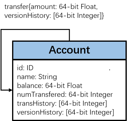
Figure 7.1: Graph schema for the ACID test queries

Figure 7.2: Hierarchy of isolation levels as described in [11]. All anomalies are covered except G-Cursor(x).

7.2 Atomicity

Atomicity ensures that either all of a transaction’s actions are performed, or none are. Two atomicity tests have been designed.

Atomicity-C

checks for every successful commit message a client receives that any data items inserted or modified are subsequently visible.

Atomicity-RB

checks for every aborted transaction that all its modifications are not visible.

Test.

(i) load a graph of Account vertices (1) each with a unique id and a set of transHistory; (ii) a client executes a full graph scan counting the number of vertices, edges and transHistory (4) using the result to initialize a counter committed; (iii) $N$transaction instances (2, 3) of the required test are then executed, committed is incremented for each successful commit; (iv) repeat the full graph scan, storing the result in the variable finalState; (v) perform the anomaly check: committed=finalState.

The Atomicity-C transaction (2) randomly selects an Account, creates a new Account, inserts a transfer edge and appends a newTrans to transHistory. The Atomicity-RB transaction (3) randomly selects an Account, appends a newTrans and attempts to insert an Account only if it does not exist. Note, for Atomicity-RB if the query API does not offer a ROLLBACK statement constraints such as vertice uniqueness can be utilized to trigger an abort.

⬇

CREATE (:Account {id: 1, name: ’AliceAcc’, transHistory: [100]}),

(:Account {id: 2, name: ’BobAcc’, transHistory: [50, 150]})

Listing 1: Cypher query for creating initial data for the Atomicity transactions.

⬇

«BEGIN»

MATCH (a1:Account {id: $account1Id})

CREATE (a1)-[t: transfer]->(a2:Account)

SET

a1.transHistory = a1.transHistory + [$newTrans],

a2.id = $account2Id,

t.amount = $newTrans

«COMMIT»

Listing 2: Atomicity-C Tx.

⬇

«BEGIN»

MATCH (a1:Account {id: $account1Id})

SET a1.transHistory = a1.transHistory + [$newTrans]

«IF» MATCH (a2: Account {id: $account2Id}) exists

«THEN» «ABORT» «ELSE»

CREATE (a2:Account {id: $account2Id})

«END»

«COMMIT»

Listing 3: Atomicity-RB Tx.

⬇

MATCH (a:Account)

RETURN count(a) AS numAccounts, count(a.name) AS numNames, sum(size(a.transHistory)) AS numTransferred

Listing 4: Atomicity-C/Atomicity-RB: counting entities in the graph.

7.3 Isolation

The gold standard isolation level is Serializability, which offers protection against all possible anomalies that can occur from the concurrent execution of transactions. Anomalies are occurrences of non-serializable behavior. Providing Serializability can be detrimental to performance [8]. Thus systems offer numerous weak isolation levels such as Read Committed and Snapshot Isolation that allow a higher degree of concurrency at the cost of potential non-serializable behavior. As such, isolation levels are defined in terms of the anomalies they prevent [8, 12]. Figure 7.2 relates isolation levels to the anomalies they proscribe.

To allow fair comparison systems must disclose the isolation level used during benchmark execution. The purpose of these isolation tests is to verify that the claimed isolation level matches the expected behavior. To this end, tests have been developed for each anomaly presented in [11]. Formal definitions for each anomaly are reproduced from [13, 11] using their system model which is described below. General design considerations are discussed before each test is described.

7.3.1 System Model

Transactions consist of an ordered sequence of read and write operations to an arbitrary set of data items, book-ended by a BEGIN operation and a COMMIT or an ABORT operation. In a graph database data items are vertices, edges and properties. The set of items a transaction reads from and writes to is termed its item read set and item write set. Each write creates a version of an item, which is assigned a unique timestamp taken from a totally ordered set (natural numbers) version $i$ of item $x$ is denoted $x_{i}$. All data items have an initial unborn version $\bot$ produced by an initial transaction $T_{\bot}$. The unborn version is located at the start of each item’s version order. Execution of transactions on a database is represented by a history, H, consisting of (i) an ordered sequence of read and write operations of each transaction, (ii) ordered data item versions read and written and (iii) commit or abort operations.  [11]

There are three types of dependencies between transactions, which capture the ways in which transactions can directly conflict. Read dependencies capture the scenario where a transaction reads another transaction’s write. Antidependencies capture the scenario where a transaction overwrites the version another transaction reads. Write dependencies capture the scenario where a transaction overwrites the version another transaction writes. Their definitions are as follows:

Read-Depends

Transaction $T_{j}$ directly read-depends (wr) on $T_{i}$ if $T_{i}$ writes some version $x_{i}$ and $T_{j}$ reads $x_{i}$.

Anti-Depends

Transaction $T_{j}$ directly anti-depends (rw) on $T_{i}$ if $T_{i}$ reads some version $x_{k}$ and $T_{j}$ writes $x$’s next version after $x_{k}$ in the version order.

Write-Depends

Transaction $T_{j}$ directly write-depends (ww) on $T_{i}$ if $T_{i}$ writes some version $x_{i}$ and $T_{j}$ writes $x$’s next version after $x_{i}$ in the version order.

Using these definitions, from a history $H$ a direct serialization graph $\textit{DSG}(H)$ is constructed. Each vertice in the DSG corresponds to a committed transaction and edges correspond to the types of direct conflicts between transactions. Anomalies can then be defined by stating properties about the DSG.

The above item-based model can be extended to handle predicate-based operations [13]. Database operations are frequently performed on a set of items provided a certain condition called the predicate, $P$ holds. When a transaction executes a read or write based on a predicate $P$, the database selects a version for each item to which $P$ applies, this is called the version set of the predicate-based denoted as $\textit{Vset}(P)$. A transaction $T_{j}$ changes the matches of a predicate-based read $r_{i}(P_{i})$ if $T_{i}$ overwrites a version in $\textit{Vset}(P_{i})$.

7.3.2 General Design

Isolation tests begin by loading a test graph into the database. Configurable numbers of write clients and read clients then execute a sequence of transactions on the database for some configurable time period. After execution, results from read clients are collected and an anomaly check is performed. In some tests, an additional full graph scan is performed after the execution period in order to collect information required for the anomaly check.

The guiding principle behind test design was the preservation of data items version history – the key ingredient needed in the system model formalization which is often not readily available to clients, if preserved at all. Several anomalies are closely related, therefore, tests had to be constructed such that other anomalies could not interfere with or mask the detection of the targeted anomaly. Test descriptions provide (i) informal and formal anomaly definitions, (ii) the required test graph, (iii) description of transaction profiles write and read clients execute, and (iv) reasoning for why the test works.

7.3.3 Dirty Write

Informally, a Dirty Write (Adya’s G0 [13]) occurs when updates by conflicting transactions are interleaved. For example, say $T_{i}$ and $T_{j}$ both modify items $\{x,y\}$. If version $x_{i}$ precedes version $x_{j}$ and $y_{j}$ precedes version $y_{i}$, a G0 anomaly has occurred. Preventing G0 is especially important in a graph database in order to maintain Reciprocal Consistency [14].

Definition.

A history $H$ exhibits phenomenon G0 if $\textit{DSG}(H)$ contains a directed cycle consisting entirely of write-dependency edges.

Test.

Load a test graph containing pairs of Account vertices connected by a transfer edge. Assign each Account a unique id and each Account and transfer edge a versionHistory property of type list (initially empty). During the execution period, write clients execute a sequence of G0 $T_{\mathrm{W}}$ instances, 5. This transaction appends its ID to the versionHistory property for each entity (2 Accounts and 1 transfer edge) in the Account pair it matches. Note, transaction IDs are assumed to be globally unique. After execution, a read client issues a G0 $T_{\mathrm{R}}$ for each Account pair in the graph, 6. Retrieving the versionHistory for each entity in an Account pair.

Anomaly check.

For each Account pair in the test graph: (i) prune each versionHistory list to remove any version numbers that do not appear in all lists; needed to account for interference from Lost Update anomalies (Section 7.3.8), (ii) compare the contents of each entities’ versionHistory list element-wise, (iii) if lists do not agree, a G0 anomaly has occurred.

Why it works.

Each successful G0 $T_{\mathrm{W}}$ creates a new version of an Account pair. Appending the transaction ID preserves the version history of each entity in the Account pair. In a system that prevents G0, each entity of the Account pair should experience the same updates, in the same order. Hence, each position in the versionHistory lists should be equivalent. The additional pruning step is needed as Lost Updates overwrites a version, effectively erasing it from the history of a data item.

⬇

MATCH

(a1:Account {id: $account1Id})

-[t:transfer]->(a2:Account {id: $account2Id})

SET a1.versionHistory = a1.versionHistory + [$tid]

SET a2.versionHistory = a2.versionHistory + [$tid]

SET t.versionHistory = t.versionHistory + [$tId]

Listing 5: Dirty Write (G0) $T_{\mathrm{W}}$.

⬇

MATCH (a1:Account {id: $account1Id})

-[t:transfer]->(a2:Account {id: $account2Id})

RETURN

a1.versionHistory AS a1VersionHistory,

t.versionHistory AS tVersionHistory,

a2.versionHistory AS a2VersionHistory

Listing 6: Dirty Write (G0) $T_{\mathrm{R}}$.

7.3.4 Dirty Reads

Aborted Reads

Informally, an Aborted Read (G1a) anomaly occurs when a transaction reads the updates of a transaction that later aborts.

Definition.

A history $H$ exhibits phenomenon G1a if $H$ contains an aborted transaction $T_{a}$ and a committed transaction $T_{c}$ such that $T_{c}$ reads a version written by $T_{a}$.

Test.

Load a test graph containing only Account vertices into the database. Assign each Account a unique id and balance initialized to 99 (or any odd number). During execution, write clients execute a sequence of G1a $T_{\mathrm{W}}$ instances, 7. Selecting a random Account id to populate each instance. This transaction attempts to set balance=200 (or any even number) but always aborts. Concurrently, read clients execute a sequence of G1a $T_{\mathrm{R}}$ instances, 8. This transaction retrieves the balance property of an Account. Read clients store results, which are collected after execution has finished.

Anomaly check.

Each read should return balance=99 (or any odd number). Otherwise, a G1a anomaly has occurred.

Why it works.

Each transaction that attempts to set balance to an even number always aborts. Therefore, if a transaction reads balance to be an even number, it must have read the write of an aborted transaction.

⬇

MATCH (a:Account {id: $accountId})

SET a.balance = 200

«SLEEP($sleepTime)»

«ABORT»

Listing 7: Aborted Read (G1a) $T_{\mathrm{W}}$.

⬇

MATCH (a:Account {id: $accountId})

RETURN a.balance as aBalance

Listing 8: Aborted Read (G1a) $T_{\mathrm{R}}$.

⬇

MATCH (a:Account {id: $accountId})

SET a.balance = $even

«SLEEP($sleepTime)»

SET a.balance = $odd

Listing 9: Interm. Read (G1b) $T_{\mathrm{W}}$.

⬇

MATCH (a:Account {id: $accountId})

RETURN a.balance as aBalance

Listing 10: Interm. Read (G1b) $T_{\mathrm{R}}$.

Intermediate Reads

Informally, an Intermediate Read (Adya’s G1b [13]) anomaly occurs when a transaction reads the intermediate modifications of other transactions.

Definition.

A history $H$ exhibits phenomenon G1b if $H$ contains a committed transaction $T_{i}$ that reads a version of an object $x_{m}$ written by transaction $T_{j}$, and $T_{j}$ also wrote a version $x_{n}$ such that $m<n$ in $x$’s version order.

Test.

Load a test graph containing only Account vertices into the database. Assign each Account a unique id and balance initialized to 99 (or any odd number). During execution, write clients execute a sequence of G1b $T_{\mathrm{W}}$ instances, 9. This transaction sets balance to an even number, then an odd number before committing. Concurrently read-clients execute a sequence of G1b $T_{\mathrm{R}}$ instances, 10. Retrieving balance property of an Account. Read clients store results which are collected after execution has finished.

Anomaly check.

Each read of balance should be an odd number. Otherwise, a G1b anomaly has occurred.

Why it works.

The final balance modified by an G1b $T_{\mathrm{W}}$ instance is never an even number. Therefore, if a transaction reads balance to be an even number it must have read an intermediate balance.

Circular Information Flow

Informally, a Circular Information Flow (Adya’s G1c [13]) anomaly occurs when two transactions affect each other; both transactions write data the other reads. For example, transaction $T_{i}$ reads a write by transaction $T_{j}$ and transaction $T_{j}$ reads a write by $T_{i}$.

Definition.

A history $H$ exhibits phenomenon G1c if $\textit{DSG}(H)$ contains a directed cycle that consists entirely of read-dependency and write-dependency edges.

Test.

Load a test graph containing only Account vertices into the database. Assign each Account a unique id and balance initialized to 0. Read-write clients are required for this test, executing a sequence of G1c $T_{\mathrm{RW}}$, 11. This transaction selects two different Account vertices, setting the balance of one Account to the transaction ID and retrieving the balance from the other. Note, transaction IDs are assumed to be globally unique. Transaction results are stored in format (txn.id, balanceRead) and collected after execution.

Anomaly check.

For each result, check the result of the transaction the balanceRead corresponds to, did not read the transaction of that result. Otherwise, a G1c anomaly has occurred.

Why it works.

Consider the result set: {($T_{\mathrm{1}}$, $T_{\mathrm{2}}$), ($T_{\mathrm{2}}$, $T_{\mathrm{3}}$), ($T_{\mathrm{3}}$, $T_{\mathrm{2}}$)}. $T_{\mathrm{1}}$ reads the balance written by $T_{\mathrm{2}}$ and $T_{\mathrm{2}}$ reads the balance written by $T_{\mathrm{3}}$. Here information flow is unidirectional from $T_{\mathrm{1}}$ to $T_{\mathrm{2}}$. However, $T_{\mathrm{2}}$ reads the balance written by $T_{\mathrm{3}}$ and $T_{\mathrm{2}}$ reads the balance written by $T_{\mathrm{3}}$. Here information flow is circular from $T_{\mathrm{2}}$ to $T_{\mathrm{3}}$ and $T_{\mathrm{3}}$ to $T_{\mathrm{2}}$. Thus a G1c anomaly has been detected.

⬇

MATCH (a1:Account {id: $account1Id}) SET a1.balance = $transactionId

MATCH (a2:Account {id: $account2Id}) RETURN a2.balance AS account2Balance

Listing 11: G1c $T_{\mathrm{RW}}$.

7.3.5 Cut Anomalies

Item-Many-Preceders

Informally, an Item-Many-Preceders (IMP) anomaly [12] occurs if a transaction observes multiple versions of the same item (transaction $T_{i}$ reads versions $x_{1}$ and $x_{2}$). In a graph database, this can be multiple reads of a vertice, edge, property or label. Local transactions (involving a single data item) occur frequently in graph databases, in “Find properties of entities” TSR 1.

Definition.

A history $H$ exhibits IMP if $\textit{DSG}(H)$ contains a transaction $T_{i}$ such that $T_{i}$ directly item-read-depends on $x$ by more than one other transaction.

Test.

Load a test graph containing Account vertices. Assign each Account a unique id and balance initialized to 1. During execution write clients execute a sequence of IMP $T_{\mathrm{W}}$ instances, 12. Selecting a random id and setting a new balance (globally unique) of the Account. Concurrently read clients execute a sequence of IMP $T_{\mathrm{R}}$ instances, 13. Performing multiple reads of the same Account; We can inject some wait time between reads to make conditions more favorable for detecting an anomaly. Both reads within an IMP $T_{\mathrm{R}}$ transaction are returned, stored and collected after execution.

Anomaly check.

Each IMP $T_{\mathrm{R}}$ result set (firstRead, secondRead) should contain the same Account balance. If not, an IMP anomaly has occurred.

Why it works.

By performing successive reads within the same transaction this test checks that a system ensures consistent reads of the same data item. If the read balance changes then a concurrent transaction has modified the data item and the reading transaction is not protected from this change.

⬇

MATCH (a:Account {id: $accountId})

SET a.balance = $newBalance

Listing 12: IMP $T_{\mathrm{W}}$.

⬇

MATCH (a1:Account {id: $accountId})

WITH a1.balance AS firstRead

«SLEEP($sleepTime)»

MATCH (a2:Account {id: $accountId})

RETURN firstRead,

a2.balance AS secondRead

Listing 13: IMP $T_{\mathrm{R}}$.

⬇

MATCH (a1:Account {id: $account1Id}), (a2:Account {id: $account2Id})

CREATE (a1)-[:transfer]->(a2)

Listing 14: PMP $T_{\mathrm{W}}$.

⬇

MATCH (a2:Account {id: $accountId})<-[:transfer]-(a1:Account)

WITH count(a1) AS firstRead

«SLEEP($sleepTime)»

MATCH (a4:Account {id: $accountId})<-[:transfer]-(a3:Account)

RETURN firstRead,

count(a3) AS secondRead

Listing 15: PMP $T_{\mathrm{R}}$.

Predicate-Many-Preceders

Informally, a Predicate-Many-Preceders (PMP) anomaly [12] occurs if a transaction observes different versions resulting from the same predicate read ($T_{i}$ reads $\textit{Vset}(P_{i})=\{x_{1}\}$ and $\textit{Vset}(P_{i})=\{x_{1},y_{2}\}$). Pattern matching is a common predicate read operation in a graph database.

Definition.

A history $H$ exhibits the phenomenon PMP if, for all predicate-based reads $r_{i}(P_{i}:\textit{Vset}(P_{i}))$ and $r_{j}(P_{j}:\textit{Vset}(P_{j}))$ in $T_{k}$ such that the logical ranges of $P_{i}$ and $P_{j}$ overlap (call it $P_{o}$), the set of transactions that change the matches of $P_{o}$ for $r_{i}$ and $r_{j}$ differ.

Test.

Load a test graph containing Account vertices. Assign each Account a unique id. During execution write clients execute a sequence of PMP $T_{\mathrm{W}}$ instances, inserting a transfer edge between a randomly selected pair of Accounts, shown in 14. Concurrently read clients execute a sequence of PMP $T_{\mathrm{R}}$ instances, 15. Performing multiple reads of the pattern (a2:Account)<-[:transfer]-(a1:Account) and counting the number of transfer edges; successive reads can be separated by some artificially injected wait time to make conditions more favorable for detecting an anomaly. Both predicates reads within a PMP $T_{\mathrm{R}}$ transaction are returned, stored and collected after test execution.

Anomaly check.

For each PMP $T_{\mathrm{R}}$ transaction result set (firstRead, secondRead), the firstRead should be equal to secondRead. Otherwise, a PMP anomaly has occurred.

Why it works.

By performing successive predicate reads and counting the number of transfer edges within the same transaction this test checks that a system ensures consistent reads of the same predicate. If the number of transfer edges changes then a concurrent transaction has inserted a new transfer edge and the reading transaction is not protected from this change.

7.3.6 Observed Transaction Vanishes

Informally, an Observed Transaction Vanishes (OTV) anomaly [12] occurs when a transaction observes part of another transaction’s updates but not all of them ($T_{1}$ writes $x_{1}$ and $y_{1}$ and $T_{2}$ reads $x_{1}$ and $y_{\bot}$). Before formally defining OTV the Unfolded Serialization Graph (USG) must be introduced [13]. The USG is specified for an individual transaction, $T_{i}$ and a history, $H$ and is denoted by $\textit{USG}(H,T_{i})$. In a USG the $T_{i}$ vertice is split into multiple vertices, one for each action read $r_{i}(\cdot)$ or write $w_{i}(\cdot)$ within the transaction. The dependency edges are now incident on the relevant event of $T_{i}$. Additionally, actions within $T_{i}$ are connected by an order edge if $T_{i}$ reads object $y_{j}$ then immediately writes on object $x$ an order edge exists from $w_{i}(x_{i})$ to $r_{i}(y_{j})$.

Definition.

A history $H$ exhibits phenomenon OTV if $\textit{USG}(H,T_{i})$ contains a directed cycle consisting of (i) exactly one read dependency edge induced by data item $x$ from $T_{j}$ to $T_{i}$ and (ii) a set of edges induced by data item $y$ containing at least one anti dependency edge from $T_{i}$ to $T_{j}$. Additionally, $T_{i}$’s read from $y$ precedes its read from $x$.

Test.

Load a test graph containing a set of cycles of length 4 of Accounts connected by transfer edges. Assign each Account an id, and balance property (initialized to 1). Note, id must be unique across vertices. During execution write clients select an id and executes a sequence of OTV $T_{\mathrm{W}}$ instances, 16. This transaction effectively creates a new version of a given cycle. Concurrently read-clients execute a sequence of OTV $T_{\mathrm{R}}$ instances, 17. Matching a given cycle and performing multiple reads. Both reads within an OTV $T_{\mathrm{R}}$ are returned, stored and collected after execution.

Anomaly check.

For each OTV $T_{\mathrm{R}}$ result set (firstRead,secondRead), the maximum balance in the firstRead should be less than or equal to the minimum balance in the secondRead. Otherwise, an OTV anomaly has occurred.

Why it works.

OTV $T_{\mathrm{W}}$ installs a new version of a cycle by updating the balance property of each Account. Therefore when matching a cycle once a transaction has observed some balance it should at least observe this same balance for every remaining entity in the cycle. Unfortunately, this cannot be deduced from a single read of the cycle as results from matching cycles often do not preserve the order in which graph entities were read. This is solved by making multiple reads of the cycle. The maximum balance of the firstRead determines the minimum balance of secondRead. If this condition is violated then a transaction has observed the effects of a transaction in the firstRead then subsequently failed to observe it in the secondRead – the observed transaction has vanished!

⬇

MATCH path =

(n:Account {id: $accountId})

-[:transfer*..4]->(n)

UNWIND nodes(path)[0..4] AS a

SET a.balance = a.balance + 1

Listing 16: OTV/FR $T_{\mathrm{W}}$.

⬇

MATCH p1 = (a1:Account {id: $accountId})-[:transfer*..4]->(a1)

RETURN extract(a IN nodes(p1) | a.balance) AS firstRead

«SLEEP($sleepTime)»

MATCH p2 = (a2:Account {id: $accountId})-[:transfer*..4]->(a2)

RETURN extract(a IN nodes(p2) | a.balance) AS secondRead

Listing 17: OTV/FR $T_{\mathrm{R}}$.

7.3.7 Fractured Read

This section is the same as LDBC SNB [1, 2], except the schema design.

Informally, a Fractured Read (FR) anomaly [11] occurs when a transaction reads across transaction boundaries. For example, if $T_{1}$ writes $x_{1}$ and $y_{1}$ and $T_{3}$ writes $x_{3}$. If $T_{2}$ reads $x_{1}$ and $y_{1}$, then repeats its read of $x$ and reads $x_{3}$ a fractured read has occurred.

Definition.

A transaction $T_{j}$ exhibits phenomenon FR if transaction $T_{i}$ writes versions $x_{a}$ and $y_{b}$ (in any order, where $x$ and $y$ may or may not be distinct items), $T_{j}$ reads version $x_{a}$ and version $y_{c}$, and $c<b$.

Test.

Same as the OTV test.

Anomaly check.

For each FR $T_{\mathrm{R}}$ (17) result set (firstRead, secondRead), all balance across both balance sets should be equal. Otherwise, an FR anomaly has occurred.

Why it works.

FR $T_{\mathrm{W}}$ writes a new version of a cycle by updating the balance properties on each Account. When FR $T_{\mathrm{R}}$ observes a balance every subsequent read in that cycle should read the same balance as FR $T_{\mathrm{W}}$ (16) installs the same balance for all Account vertices in the cycle. Thus, if it observes a different balance it has observed the effect of a different transaction and has read across transaction boundaries.

7.3.8 Lost Update

Informally, a Lost Update (LU) anomaly [11] occurs when two transactions concurrently attempt to make conditional modifications to the same data item(s).

Definition.

A history $H$ exhibits phenomenon LU if $\textit{DSG}(H)$ contains a directed cycle having one or more anti-dependency edges and all edges are induced by the same data item $x$.

Test.

Load a test graph containing Account vertices. Assign each Account a unique id and a property numTransferred (initialized to 0). During execution write clients execute a sequence of LU $T_{\mathrm{W}}$ instances, 18. Choosing a random Account and incrementing its numTransferred property. Clients store local counters (expNumTransferred) for each Account, which is incremented each time an Account is selected and the LU $T_{\mathrm{W}}$ instance successfully commits. After the execution period, the numTransferred is retrieved for each Account using LU $T_{\mathrm{R}}$ in 19 and expNumTransferred are pooled from write clients for each Account.

Anomaly check.

For each Account its numTransferred property should be equal to the (global) expNumTransferred for that Account.

Why it works.

Clients know how many successful LU $T_{\mathrm{W}}$ instances were issued for a given Account. The observable numTransferred should reflect this ground truth, otherwise, a LU anomaly must have occurred.

⬇

MATCH (a1:Account {id: $account1Id})

CREATE (a1)-[:transfer]->(a2:Account {id: $account2Id})

SET a1.numTransferred = a1.numTransferred + 1

RETURN a1.numTransferred

Listing 18: Lost Update $T_{\mathrm{W}}$.

⬇

MATCH (a:Account {id: $accountId})

OPTIONAL MATCH (a)-[t:transfer]->()

WITH a, count(t) AS numTransferEdges

RETURN numTransferEdges,

a.numTransferred AS numTransferred

Listing 19: Lost Update $T_{\mathrm{R}}$.

7.3.9 Write Skew

This section is similar to LDBC SNB [1, 2], except the schema design and constraint: a1.id % 2 = 1 in WS $T_{\mathrm{R}}$, 21.

Informally, Write Skew (WS) occurs when two transactions simultaneously attempted to make disjoint conditional modifications to the same data item(s). It is referred to as G2-Item in [13, 15].

Definition.

A history $H$ exhibits WS if $\textit{DSG}(H)$ contains a directed cycle having one or more anti-dependency edges.

Test.

Load a test graph containing $n$ pairs of Account vertices (a1, a2) for $k=0,\ldots,n-1$, where the $k$th pair gets IDs a1.id = 2*k+1 and a2.id = 2*k+2, and balances a1.balance = 70 and a2.balance = 80. There is a constraint: a1.balance + a2.balance > 0. During execution write clients execute a sequence of WS $T_{\mathrm{W}}$ instances, 20. Selecting a random Account pair and decrementing the value property of one Account provided doing so would not violate the constraint. After execution the database is scanned using WS $T_{\mathrm{R}}$, 21.

Anomaly check.

For each Account pair the constraint should hold true, otherwise, a WS anomaly has occurred.

Why it works.

Under no Serializable execution of WS $T_{\mathrm{W}}$ instances would the constraint a1.balance + a2.balance > 0 be violated. Therefore, if WS $T_{\mathrm{R}}$ returns a violation of this constraint it is clear a WS anomaly has occurred.

⬇

MATCH (a1:Account {id: $account1Id}),

(a2:Account {id: $account2Id})

«IF a1.balance + a2.balance < 100)» «THEN» «ABORT» «END»

«SLEEP($sleepTime)»

account = «pick randomly between account1Id, account2Id»

MATCH (a:Account {id: $account})

SET a.balance = a.balance - 100

«COMMIT»

Listing 20: WS $T_{\mathrm{W}}$.

⬇

MATCH (a1:Account),

(a2:Account {id: a1.id+1})

WHERE a1.balance + a2.balance <= 0

and a1.id % 2 = 1

RETURN a1.id AS a1id,

a1.balance AS a1balance,

a2.id AS a2id,

a2.balance AS a2balance

Listing 21: WS $T_{\mathrm{R}}$.

7.4 Consistency and Durability Tests

While this chapter mainly focused on atomicity and isolation from the ACID properties, we provide a short overview of consistency and durability.

Durability is a hard requirement for FinBench Transaction and checking it is part of the auditing process. The durability test requires the execution of the LDBC FinBench transaction workload and uses the LDBC FinBench driver. Note, the database and the driver must be configured in the same way as would be used in the performance run. The durability test is executed as follows:

1. Execute the LDBC FinBench transaction workload;

2. After 2 hours of execution, terminate all database processes ungracefully. This can be done by shutting down the entire machines or killing processes forcefully. Note, the ungraceful shutdown on different machines may differ:

   1. Amazon Web Services: Using the AWS CLI to force stop the instance: aws ec2 stop-instances --instance-ids {ID} --force;

   2. Alibaba Cloud: Stopping the instance by Force Stop option on the ECS Console;

   3. Bare Metal: Force stop the machine by poweroff -f. Note, shutdown -h now or shutdown -r now are graceful;

   4. Others: Depends on discussion.

3. Restart the database system, retrieve the last entities (vertices or edges) updated by the last update operations before the crash from the driver logs;

4. Issue read queries to get the value of the last entities. If the returned data matches the committed data according to the logs, the system passes the durability test.

Consistency is defined in terms of constraints: the database remains consistent under updates; i.e. no constraint is violated. Relational database systems usually support primary- and foreign-key constraints, as well as domain constraints on column values and sometimes also support simple within-row constraints. Graph database systems have a diversity of interfaces and generally do not support constraints, beyond sometimes domain and primary key constraints (in case indices are supported). However, we do note that we anticipate that graph database systems will evolve to support constraints in the future. Beyond equivalents of the relational ones, property graph systems might introduce graph-specific constraints, such as (partial) compliance to a schema formulated on top of property graphs, rules that guide the presence of labels or structural graph constraints such as connectedness of the graph, absence of cycles, or arbitrary well-formedness constraints [16]. Here we provide an example of a consistency test (the consistency test also requires the execution of the LDBC FinBench transaction workload and uses the LDBC FinBench driver):

1. Add some precomputed properties (similar to materialized views) for vertex or edge. i.e. add property balance for account, which maintains the balance of the given account according to the associated transactions, and at the same time, the update queries need to be modified to maintain the balance. You can also design other constraints(i.e. vertice uniqueness);

2. Execute the LDBC FinBench transaction workload;

3. After 1 hour of execution, pause the execution of the workload; Issue read queries to check if the constraints are consistent after updating;

4. Resume the execution of the workload. After another 1 hour of execution, terminate all database processes ungracefully;

5. Restart the database system, Issue read queries to check if the constraints are consistent after recovery;

6. If both of the above checks pass, the system passes the consistency test.

Chapter 8 Auditing Rules

This chapter contains the auditing policies for the LDBC Benchmarks. The initial draft of the auditing policies was published in the EU project deliverable D6.3.3 “LDBC Benchmark Auditing Policies”.

This chapter is divided into the following parts:

• Motivation of benchmark result auditing

• General discussion of auditable aspects of benchmarks

• Specific checklists and running rules for LDBC FinBench workloads

Many definitions and general considerations are shared between the benchmarks, hence it is justified to present the principles first and to refer to these in the context of the benchmark-specific rules. The auditing process, including the auditor certification exams, the possibility of challenging audited results, , are defined in the LDBC Byelaws [7]. Please refer to the latest Byelaws document when conducting audits.

8.1 Rationale and General Principles

The purpose of benchmark auditing is to improve the credibility and reproducibility of benchmark claims by involving a set of detailed execution rules and third-party verification of compliance with these.

Rules may exist separately from auditing but auditing is not meaningful unless the rules are adequately precise. Aspects like auditor training and qualification cannot be addressed separately from a discussion of the matters the auditor is supposed to verify. Thus, the credibility of the entire process hinges on a clear and shared understanding of what a benchmark is expected to demonstrate and on the auditor being capable of understanding the process and verifying that the benchmark execution is fair and does not abuse the rules or pervert the objectives of the benchmark.

Due to the open-ended nature of technology and the agenda of furthering innovation via measurement, it is not feasible or desirable to over-specify the limits of benchmark implementation. Hence, there will always remain judgment calls for borderline cases. In this respect auditing and the LDBC are not separate. It is expected that issues of compliance, as well as maintenance of rules, will come before the LDBC as benchmark claims are made.

8.2 Auditing Rules Overview

8.2.1 Auditor Training, Certification, and Selection

8.2.1.1 Auditor Training

Auditor training consists of familiarization with the benchmark and existing implementations thereof. This involves the auditor candidate running the reference implementations of the benchmark to see what is normal behavior and practice in the workload. The training and practice may involve communication with the benchmark task force for clarifying the intent and details of the benchmark rules. This produces feedback for the task force for further specification of the rules.

8.2.1.2 Auditor Certification

The auditor certification and qualification are done in the form of an examination administered by the task force responsible for the benchmark being audited. The examination may be carried out by teleconference. The task force will subsequently vote on accepting each auditor, by a simple majority. An auditor is certified for a particular benchmark by the task force maintaining the benchmark in question.

8.2.1.3 Auditor Selection

In the default auditor selection, the task force responsible for the benchmark being audited appoints a third-party, impartial auditor. If needed, a Conflict of Interest Statement will be signed and provided. The task force may in special cases appoint itself as auditor of a particular result. This is not, however, the preferred course of action but may be done if no suitable third-party auditor is available.

8.2.2 Auditing Process Stages

8.2.2.1 Getting Ready for a Benchmark Audit

A benchmark result can be audited if it is a complete implementation of an LDBC benchmark workload. This includes implementing all operations correctly, using official data sets, using the official LDBC driver (if available), and complying with the auditing rules of the workload (workloads may have different rules regarding query languages, the allowance of materialized views, ). Workloads may specify further requirements such as ACID compliance (checked using the LDBC FinBench ACID test suite).

8.2.2.2 Performing a Benchmark Audit

A benchmark result is to be audited by an LDBC-appointed auditor or the LDBC task force managing the benchmark. An LDBC audit may be performed by remote login and does not require the auditor’s physical presence on site. The test sponsor shall grant the auditor any access necessary for validating the benchmark run. This will typically include administrator access to the SUT hardware.

8.2.2.3 Benchmark-Specific Checklist

Each benchmark specifies a checklist to be verified by the auditor. The benchmark run shall be performed by the auditor. The auditor shall make copies of relevant configuration files and test results for future checking and insertion into the full disclosure report.

8.2.2.4 Producing the FDR

The FDR is produced by the auditor or auditors, with any required input from the test sponsor. Each non-default configuration parameter needs to be included in the FDR and justification needs to be provided why the given parameter was changed. The auditor produces an attestation letter that verifies the authenticity of the presented results. This letter is to be included in the FDR as an addendum. The attestation letter has no specific format requirements but shall state that the auditor has established compliance with a specified version of the benchmark specification.

8.2.2.5 Publishing the FDR

The FDR and any benchmark-specific summaries thereof shall be published on the LDBC website, https://ldbcouncil.org/.

8.2.3 Challenge Procedure

A benchmark result may be challenged for non-compliance with LDBC rules. The benchmark task force responsible for the maintenance of the benchmark will rule on matters of compliance. A result found to be non-compliant will be withdrawn from the list of official LDBC benchmark results.

8.3 Auditable Properties of Systems and Benchmark Implementations

8.3.1 Validation of Query Results

A benchmark should be published with a deterministically reproducible validation data set. Validation queries applied to the validation data set will deterministically produce a set of correct answers. This is used in the first stage of the benchmark run to test for the correctness of A SUT or benchmark implementation. This validation stage is not timed.

Inputs for validation

The validation takes the form of a set of data generator parameters, a set of test queries that at least include one instance of each of the workload query templates and the expected results.

Approximate results and error margin

In certain cases, the results may be approximate. This may happen in cases of non-unique result ordering keys, imprecise numeric data types, random behaviors in certain graph analytics algorithms etc. Therefore, a validation set shall specify the degree of allowable error: For example, for counts, the value must be exact, for sums, averages and the like, at least 8 significant digits are needed, for statistical measures like graph centralities, the result must be within 1% of the reference result. Each benchmark shall specify its expectation in an unambiguously verifiable manner.

8.3.2 ACID Compliance

As part of the auditing process for the Transaction workload, the auditors ascertain that the SUT satisfies the ACID properties, it provides atomic transactions, complies with its claimed isolation level, and ensures durability in case of failures. This section outlines the transactional behaviors of SUTs which are checked in the course of auditing A SUT in a given benchmark.

A benchmark specifies transactional semantics that may be required for different parts of the workload. The requirements will typically be different for the initial bulk load of data and for the workload itself. Different sections of the workload may further be subject to different transactionality requirements.

No finite series of tests can prove that the ACID properties are fully supported. Passing the specified tests is a necessary, but not sufficient, condition for meeting the ACID requirements. However, for fairness of reporting, only the tests specified here are required and must appear in the FDR for a benchmark. (This is taken exactly from the TPC-C specification [tpcc].)

The properties for ACID compliance are defined as follows:

Atomicity

Either all the effects of the transaction are in effect after the transaction or none of the effects is in effect. This is by definition only verifiable after a transaction has finished.

Consistency

ADS such as secondary indices will be consistent among themselves as well as with the table or other PDS, if any. Such a consistency (compliance to all constraints, if these are declared in the schema, primary key constraint, foreign key constraints and cardinality constraints) may be verified after the commit or rollback of a transaction. If a single thread of control runs within a transaction, then subsequent operations are expected to see a consistent state across all data indices of a table or similar object. Multiple threads which may share a transaction context are not required to observe a consistent state at all times during the execution of the transaction. Consistency will however always be verifiable after the commit or rollback of any transaction, regardless of the number of threads that have either implicitly or explicitly participated in the transaction. Any intra-transaction parallelism introduced by the SUT will preserve transactional semantics statement-by-statement. If explicit, application created sessions share a transaction context, then this definition of consistency does not hold: for example, if two threads insert into the same table at the same time in the same transaction context, these may or may not see a consistent image of (E)ADS for the parts affected by the other thread. All things will be consistent after the commit or rollback, however, regardless of the number of threads, implicit or explicit that have participated in the transaction.

Isolation

Isolation is defined as the set of phenomena that may (or may not) be observed by operations running within a single transaction context. The levels of isolation are defined as follows:

Read uncommitted

No guarantees apply.

Read committed

A transaction will never read a value that has at no point in time been part of a committed state.

Repeatable read

If a transaction reads a value several times during its execution, then it will see the original state with its modifications so far applied to it. If the transaction itself consists of multiple reading and updating threads then the ambiguities that may arise are beyond the scope of transaction isolation.

Serializable

The transactions see values that correspond to a fully serial execution of all client transactions. This is like a repeatable read except that if the transaction reads something, and repeats the read, it is guaranteed that no new values will appear for the same search condition on a subsequent read in the same transaction context. For example, a row that was seen not to exist when first checked will not be seen by a subsequent read. Likewise, counts of items will not be seen to change.

Durability

Durability means that once the SUT has confirmed a successful commit, the committed state will survive any instantaneous failure of the SUT (a power failure, software crash, reboot or the like). Durability is tied to atomicity in that if one part of the changes made by a transaction survives then all parts must survive.

8.3.3 Data Format and Preprocessing

When producing the data sets, implementers are allowed to use custom formatting options (use or omission of quotes, separator character, datetime format, ). It is also allowed to convert the output of the DataGen into a format (Parquet) that is loadable by the test-specific implementation of the data importer. Additional preprocessing steps are also allowed, including adjustments to the CSV files (with shell scripts), splitting and concatenating files, compressing and decompressing files, However, the preprocessing step shall not include a precomputation of (partial) query results.

8.3.4 Query Languages

In typical RDBMS benchmarks, online transaction processing (OLTP) benchmarks are allowed to be implemented via stored procedures, effectively amounting to explicit query plans. Meanwhile, online analytical processing (OLAP) benchmarks prohibit the use of using general-purpose programming languages (C, C++, Java) for query implementations and only allow domain-specific query languages.

In the graph processing space, there is currently (as of 2022) no standard query language and the systems are considerably more heterogeneous. Therefore, the LDBC situation regarding declarative is not as simple as that of for example the TPC-H (where queries should be specified in SQL with the additional constraint of omitting any hints for OLAP workloads) and individual FinBench workloads specify their policy of either requiring a domain-specific query language or allowing the implementation of the queries in a general-purpose programming language.

In the case of domain-specific languages, systems are allowed to implement a FinBench query as a sequence of multiple queries. A typical example of this is the following sequence: (1) create a projected graph, (2) run query, (3) drop projected graph. However, it is not allowed to use sub-queries in an unrealistic and contrived manner, the goal of overcoming optimization issues, hard-coding a certain join order in a declarative query language. It is the responsibility of the auditor to determine whether a sequence of queries can be considered realistic w.r.t. how a user would formulate their queries in the language provided by the system.

8.3.4.1 Rules for Imperative Implementations Using a General-Purpose Programming Language

An implementation where the queries are written in a general-purpose programming language (including imperative and “API-based” implementations) may choose between semantically equivalent implementations of an operation based on the query parameters. This simulates the behavior of a query optimizer in the presence of literal values in the query. If an implementation does this, all the code must be disclosed as part of the FDR and the decision must be based on values extracted from the database, not on hard-coded threshold values in the implementation.

The auditor must be able to reliably assess the compliance of implementation to guidelines specifying these matters. The actual specification remains benchmark-dependent. Borderline cases may be brought to the task force responsible for arbitration.

8.3.4.2 Disclosure of Query Implementations in the FDR

Benchmarks allowing imperative expression of workload should require full disclosure of all query implementation code.

8.3.5 Materialization

The mix of read and update operations in a workload will determine to which degree precomputation of results is beneficial. The auditor must check that materialized results are kept consistent at the end of each transaction.

8.3.6 System Configuration and System Pricing

A benchmark execution shall produce a full disclosure report which specifies the hardware and software of the SUT, the benchmark implementation version and any specifics that are detailed in the benchmark specification. This clause gives a general minimum for disclosure for the SUT.

8.3.6.1 Details of Machines Driving and Running the Workload

A SUT may consist of one or more pieces of physical hardware. A SUT may include virtual or bare-metal machines in a cloud service. For each distinct configuration, the FDR shall disclose the number of units of the type as well as the following:

1. The used cloud provider (including the region where machines reside, if applicable).

2. Common name of the item, Dell PowerEdge xxxx or i3.2xlarge instance.

3. Type and number of CPUs, cores & threads per CPU, clock frequency, cache size.

4. Amount of memory, type of memory and memory frequency, 64GB DDR3 1333MHz.

5. Disk controller or motherboard type if the disk controller is on the motherboard.

6. For each distinct type of secondary storage device, the number and specification of the device, 4xSeagate Constellation 2TB SATA 6Gbit/s.

7. Number and type of network controllers, 1x Mellanox QDR InfiniBand HCA, PCIE 2.0, 2x1GbE on motherboard. If the benchmark execution is entirely contained on a single machine, it must be stated, and the description of network controllers can be omitted.

8. Number and type of network switches. If multiple switches are used, the wiring between the switches should be disclosed. Only the network switches and interfaces that participate in the run need to be reported. If the benchmark execution is entirely contained on a single machine, it must be stated, and the description of network switches can be omitted.

9. Date of availability of the system as a whole, the latest date of availability of any part.

8.3.6.2 System Pricing

The price of the hardware in question must be disclosed. For cloud setups, the price of a dedicated instance for 3 years must be disclosed. The price should reflect the single quantity list price that any buyer could expect when purchasing one system with the given specification. The price may be either an item-by-item price or a package price if the system is sold as a package. Reported prices should adhere to the TPC Pricing Specification 2.7.0 [pricing, tpc-pricing]. It is particularly important to ensure that the maintenance contract guarantees 24/7 support and 4 hour response time for problem recognition.

8.3.6.3 Details of Software Components in the System

The SUT software must be described at least as follows:

1. The units of the SUT software are typically the DBMS and operating system.

2. Name and version of each separately priced piece of the SUT software.

3. If the price of the SUT software is tied to the platform or the count of concurrent users, these parameters must be disclosed.

4. Price of the SUT software.

5. Date of availability.

Reported prices should adhere to the TPC Pricing Specification 2.5.0 [pricing, tpc-pricing].

The configuration of the SUT must be reported to include the following:

1. The used LDBC specification, driver and data generator version.

2. Complete configuration files of the DBMS, including any general server configuration files, any configuration scripts run on the DBMS for setting up the benchmark run etc.

3. Complete schema of the DBMS, including eventual specification of storage layout.

4. Any OS configuration parameters if other than default, vm.swappiness, vm.max_map_count in Linux.

5. Complete source code of any server-side logic, stored procedures, triggers.

6. Complete source code of driver-side benchmark implementation.

7. Description of the benchmark environment, including software versions, OS kernel version, DBMS version as well as versions of other major software components used for running the benchmark (Docker, Java Virtual Machine, Python, etc.).

8. The SUT’s highest configurable isolation level and the isolation level used for running the benchmark.

8.3.6.4 Audit of System Configuration

The auditor must ascertain that a reported run has indeed taken place on the SUT in the disclosed configuration. The full disclosure shall contain any relevant parameters of the benchmark execution itself, including:

1. Parameters, switches, configuration file for data generation.

2. Complete text of any data loading script or program.

3. Parameters, switches, configuration files for any test driver. If the test driver is not an LDBC supplied open source package or is a modification of such, then the complete text or diff against a specific LDBC package must be disclosed.

4. Test driver output files shall be part of the disclosure. In general, these must at least detail the following:

   1. Time and duration of data load and the timed portion of the benchmark execution.

   2. Count of each workload item (query, transaction) successfully executed within the measurement window.

   3. Min/average/max execution time of each workload item, the specific benchmark shall specify additional details.

Given this information, the number of concurrent database sessions at each point in the execution must be clearly stated. In the case of a cluster database, the possible spreading of connections across multiple server processes must be disclosed.

All parameters included in this section must be reported in the full disclosure report to guarantee that the benchmark run can be reproduced exactly in the future. Similarly, the test sponsor will inform the auditor of the scale factor to test. Finally, a clean test system with enough space to store the initial data set, the update streams, substitution parameters and anything that is part of the input and output as well as the benchmark run must be provided.

8.3.7 Benchmark Specifics

Similarly to TPC benchmarks, the LDBC benchmarks prohibit so-called benchmark specials (extra software modules implemented in the core DBMS logic just to make a selected benchmark run faster are disallowed). Furthermore, upon request of the auditor, the test sponsor must provide all the source codes relevant to the benchmark.

8.4 Auditing Rules for the Transaction Workload

This section specifies a checklist (in the form of individual sections) that a benchmark audit shall cover in case of the FinBench Transaction workload. An overview of the benchmark audit workflow is shown in Figure 8.1. The three major phases of the audit are preparing the input data and validation query results (captured by Preparations in the figure), validating the correctness of query results returned by the SUT using the validation scale factor and running the benchmark with all the prescribed workloads (Benchmarking), and creating the FDR (Finalization). The color codes capture the responsibilities of performing a step or providing some data in the workflow.

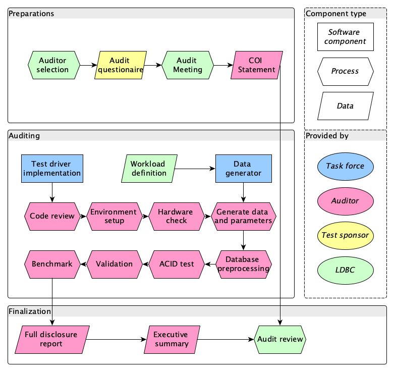
Figure 8.1: Benchmark execution and auditing workflow. For non-audited runs, the implementers perform the steps of the auditor.

A key objective of the auditing guidelines for the Transaction workload is to allow a broad range of systems to implement the benchmark. Therefore, they do not impose constraints on the data model (graph, relational, triple, representations are allowed) or on the query language (both declarative and imperative languages are allowed).

8.4.1 Scaling Factors

The scale factor of a FinBench data set is the size of the data set in GiB of CSV (comma-separated values) files. The size of a data set is characterized by scale factors: SF0.1, SF1, SF3 (see Section 3.4.2). All data sets contain data for three years of financial activities.

The validation run shall be performed on the SF1 data set (see Section 8.4.6.1). Note that the auditor may perform additional validation runs of the benchmark implementation using smaller data sets (SF1) and issue queries.

Audited benchmark runs of the Transaction workload shall use SF10. The rationale behind this decision is to ensure that there is a sufficient number of update operations available to guarantee 2.5 hours of continuous execution (see Section 8.4.7.2).

8.4.2 Data Model

FinBench may be implemented with different data models (relational, RDF, and different graph data models). The reference schema is provided in the specification using a UML-like notation.

8.4.3 Precomputation

Precomputation of query results (both interim and end results) is allowed. However, systems must ensure that precomputed results (materialized views) are kept consistent upon updates.

8.4.4 Benchmark Software Components

LDBC provides a test driver, data generator, and summary reporting scripts. Benchmark implementations shall use a stable version of the test driver. The SUT’s database software should be a stable version that is available publicly or can be purchased at the time of the release of the audit. Please see Section 1.4 for more details.

8.4.4.1 Adaptation of the Test Driver to a DBMS

A qualifying run must use a test driver that adapts the provided test driver to interface with the SUT. Such an implementation, if needed, must be provided by the test sponsor. The parameter generation, result recording, and workload scheduling parts of the test driver should not be changed. The auditor must be given access to the test driver source code used in the reported run.

The test driver produces the following artifacts for each execution as a by-product of the run: Start and end timestamps in wall clock time, recorded with microsecond precision. The identifier of the operation and any substitution parameters.

8.4.4.2 Summary of Benchmark Results

A separate test summary tool provided with the test driver analyses the test driver log(s) after a measurement window is completed.

The tool produces for each of the distinct queries and transactions the following summary:

• Run time of query in wall clock time.

• Count of executions.

• Minimum/mean/percentiles/maximum execution time.

• Standard deviation from the average execution time.

The tool produces for the complete run the following summary:

• Operations per second for a given SF (throughput). This is the primary metric of this workload.

• The total execution time in wall clock time.

• The total number of completed operations.

8.4.5 Implementation Language and Data Access Transparency

The queries and updates may be implemented in a domain-specific query language or as procedural code written in a general-purpose programming language (using the API of the database).

8.4.5.1 Implementations Using a Domain-Specific Query Language

If a domain-specific query language is used, SPARQL, SQL, Cypher, or Gremlin, then explicit query plans are prohibited in all read-only queries. The update transactions may still consist of multiple statements, effectively amounting to explicit plans.

Explicit query plans include but are not limited to:

• Directives or hints specifying a join order or join type

• Directives or hints specifying an access path, which index to use

• Directives or hints specifying an expected cardinality, selectivity, fanout or any other information that pertains to the expected number of results or cost of all or part of the query.

Rationale behind the applied restrictions. The updates are effectively OLTP and, therefore, the customary freedoms apply, including the use of stored procedures, however subject to access transparency. Declarative queries in a benchmark implementation should be such that they could plausibly be written by an application developer. Therefore, their formulation should not contain system-specific aspects that an application developer would be unlikely to know. In other words, making a benchmark implementation should not require uncommon sophistication on behalf of the developer. This is a regular practice in analytical benchmarks, TPC-H.

8.4.5.2 Implementations Using a General-Purpose Programming Language

Implementations using a general-purpose programming language for specifying the queries (including procedural, imperative, and API-based implementations) are expected to respect the rules described in Section 8.3.4. For these implementations, the rules in Section 8.4.5.1 do not apply.

8.4.6 Correctness of Benchmark Implementation

8.4.6.1 Validation data set

The scale factor 1 shall be used as a validation data set.

8.4.6.2 ACID Compliance

The Transaction workload requires full ACID support (Section 8.3.2) from the SUT. This is tested using the LDBC ACID test suite. For the specification of this test suite, see Chapter 7 and the related software repository at https://github.com/ldbc/ldbc_finbench_acid.

Expected level of isolation

If a transaction reads the database with the intent to update, the DBMS must guarantee no dirty reads. In other words, this corresponds to read committed isolation.

Durability and checkpoints

A checkpoint is defined as the operation which causes data persisted in a transaction log to become durable outside the transaction log. Specifically, this means that A SUT restart after instantaneous failure following the completion of the checkpoint may not have recourse to transaction log entries written before the end of the checkpoint.

A checkpoint typically involves a synchronization barrier at which all data committed before the moment is required to be in durable storage that does not depend on the transaction log. Not all DBMSs use a checkpoint mechanism for durability. For example, a system may rely on redundant storage of data for durability guarantees against the instantaneous failure of a single server.

The measurement window may contain a checkpoint. If the measurement window does not contain one, then the restart test will involve redoing all the updates in the window as part of the recovery test.

The timed window ends with an instantaneous failure of the SUT. Instantaneously killing all the SUT process(es) is adequate for simulating instantaneous failure. All these processes should be killed within one second of each other with an operating system action equivalent to the Unix kill -9. If such is not available, then powering down each separate SUT component that has an independent power supply is also possible.

The restart test consists of restarting the SUT process(es) and finishes when the SUT is back online with all its functionality and the last successful update logged by the driver can be seen to be in effect in the database.

If the SUT hardware was powered down, the recovery period does not include the reboot and possible file system check time. The recovery time starts when the DBMS software is restarted.

Recovery

The SUT is to be restarted after the measurement window and the auditor will verify that the SUT contains the entirety of the last update recorded by the test driver(s) as successfully committed. The driver or the implementation has to make this information available. The auditor may also check the audit log of the SUT (if available) to confirm that the operations issued by the driver were saved.

Once an official run has been validated, the recovery capabilities of the system must be tested. The system and the driver must be configured in the same way as in during the benchmark execution. After a warm-up period, execution of the benchmark will be performed under the same terms as in the previous measured run.

Measuring recovery time

At an arbitrary point close to 2 hours of wall clock time during the run, the machine will be shut down. Then, the auditor will restart the database system and will check that the last committed update (in the driver log file) is actually in the database. The auditor will measure the time taken by the system to recover from the failure. Also, all the information about how durability is ensured must be disclosed. If checkpoints are used, these must be performed for a period of 10 minutes at most.

8.4.7 Benchmarking Workflow

A benchmark execution is divided into the following processes (these processes are also shown in Figure 8.1):

Generate data

This includes running the data generator, placing the generated files in a staging area, configuring storage, setting up the SUT configuration and preparing any data partitions in the SUT. This may include preallocating database space but may not include loading any data or defining any schema having to do with the benchmark.

Preprocessing

If needed, the output from the data generator is to preprocess the data set (Section 8.3.3).

Create validation data

Using one of the reference implementations of the benchmark, the reference validation data is obtained in JSON format.

Data loading

The test sponsor must provide all the necessary documentation and scripts to load the data set into the database to test. This includes defining the database schema, if any, loading the initial database population, making this durably stored and gathering any optimizer statistics. The system under test must support the different data types needed by the benchmark for each of the attributes at their specified precision. No data can be filtered out, everything must be loaded. The test sponsor must provide a tool to perform arbitrary checks of the data or a shell to issue queries in a declarative language if the system supports it.

Run cross-validation

This step uses the data loader to populate the database, but the load is not timed. The validation data set is used to verify the correctness of the SUT. The auditor must load the provided data set and run the driver in validation mode, which will test that the queries provide the official results. The benchmarking workflow will not go beyond this point unless the results match the expected output.

Warm-up

Benchmark runs are preceded by a warm-up which must be performed using the LDBC driver.

Run benchmark

The bulk load time is reported and is equal to the amount of elapsed wall clock time between starting the schema definition and receiving the confirmation message of the end of statistics gathering. The workflow runs begin after the bulk load is completed. If the run does not directly follow the bulk load, it must start at a point in the update stream that has not previously been played into the database. In other words, a run may only include update events whose timestamp is later than the latest message creation date in the database before the start of the run. The run starts when the first of the test drivers sends its first message to the SUT. If the SUT is running in the same process as the driver, the window starts when the driver starts. Also, make sure that the -rl/--results_log is enabled. Make sure that all operations are enabled, and the frequencies are those for the selected scale factor (see the exact specification of the frequencies in Appendix B).

8.4.7.1 Query Timing During Benchmark Run

A valid benchmark run must last at least 2 hours of wall clock time and at most 2 hours and 15 minutes. In order to be valid, a benchmark run needs to meet the “95% on-time requirement”. The results_log.csv file contains the $\mathsf{actual\_start\_time}$ and the $\mathsf{scheduled\_start\_time}$ of each of the issued queries. To have a valid run, 95% of the queries must meet the following condition:

$$\mathsf{actual\_start\_time}-\mathsf{scheduled\_start\_time}<1\ \mathrm{second}$$

If the execution of the benchmark is valid, the auditor must retrieve all the files from the directory specified by --results_dir which includes configuration settings used, results log and results summary. All of which must be disclosed.

8.4.7.2 Measurement Window

Benchmark runs execute the workload on the SUT in two phases (Figure 8.2). First, the SUT must undergo a warm-up period that takes at least 30 minutes and at most 35 minutes. The goal of this is to put the system in a steady state which reflects how it would behave in a normal operating environment. The performance of the operations during warm-up is not considered. Next, the SUT is benchmarked during a two-hour measurement window. Operation times are recorded and checked to ensure the “95% on-time requirement” is satisfied.

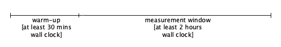
Figure 8.2: Warm-up and measurement window for the benchmark run.

The FinBench DataGen produces 3 years worth data of which 3% is used for updates (LABEL:sec:transaction-workload-data-sets), approximately $3\times 365\times 0.03=32.85~{}\text{days}=788.4~{}\text{hours}$. To ensure that the 2.5 hours wall clock period has enough input data, the lower bound of TCR is defined as 0.001 (if $2628$ hours of updates are played back at more than $1000\times$ speed, the benchmark framework runs out of updates to execute). A system that can achieve a better compression (lower TCR value) on a given scale factor should use larger SFs for their benchmark runs – otherwise their total runs will be less than 2.5 hours, making them unsuitable for auditing.

8.4.8 Full Disclosure Report

Upon successful completion of the audit, an FDR is compiled. In addition to the general requirements, the full disclosure shall cover the following:

• General terms: an executive summary and declaration of the credibility of the audit

• Conflict of Interest Statement between the auditor and the test sponsor, if needed.

• System description and pricing summary

• Data generation and data loading

• Test driver details

• Performance metrics

• Validation results

• ACID compliance

• List of supplementary materials

To ensure the reproducibility of the audited results, a supplementary package is attached to the full disclosure report. This package should contain:

• A README file with instructions specifying how to set up the system and run the benchmark

• Configuration files of the database, including database-level configuration such as buffer size and schema descriptors (if necessary)

• Source code or binary of a generic driver that can be used to interact with the DBMS

• SUT-specific LDBC driver implementation (similarly to the projects in https://github.com/ldbc/ldbc_finbench_transaction_impls)

• Script or instructions to compile the LDBC Java driver implementation

• Instructions on how to reach the server through CLI and/or web UI (if applicable), the URL (including port number), username and password

• LDBC configuration files (.properties), including the time_compression_ratio values used in the audited runs

• Scripts to preprocess the input files (if necessary) and to load the data sets into the database

• Scripts to create validation data sets and to run the benchmark

• The implementations of the queries and the update operations, including their complete source code (declarative queries specifications, stored procedures, )

• Implementation of the ACID test suite

• Binary package of the DBMS (.deb or .rpm)

Chapter 9 Related Work

A detailed list of LDBC publications is curated at https://ldbcouncil.org/publications.

LDBC FinBench is designed based on the LDBC SNB [1, 2] and introduces the new features in financial scenarios.

Appendix A Choke Points

Introduction

An interesting benchmark should be designed with representative read-world scenarios and also chokepoints embedded in the deeper technical level. Chokepoints capture particularly challenging aspects of queries. The correlations between chokepoints and read queries are displayed in Table A.1. To help understand the following chokepoints, there are some annotations.

• The capital abbreviations are short for the aspects the chokepoints affect.

  • QOPT: Those aimed at testing aspects of the query optimizer.

  • QEXE: Those aimed at testing aspects of the execution engine.

  • STORAGE: Those aimed at testing aspects of the storage system.

  • LANG: Those aimed at testing aspects of the expression capability of DSL.

  • UPD: Those aimed at testing aspects of the update operation performance.

• The gray boxes in the top right corner annotate the source of the chokepoints.

  • TPC-H means the chokepoint is from the paper TPC-H Analyzed [17]. You can refer to the paper for the chokepoint details.

  • From SNB means the chokepoint refers to the ones in LDBC SNB [2].

  • New in FinBench means the chokepoint is summarized newly from FinBench.

Table A.1: Coverage of choke points by queries.

A.1 Aggregation Performance

CP-1.1: [QOPT] Interesting orders TPC-H 1.2

This choke point tests the ability of the query optimizer to exploit the interesting orders induced by some operators. Apart from clustered indices providing key order, other operators also preserve or even induce tuple orderings. Sort-based operators create new orderings, typically on the probe-side of a hash join conserves its order, etc.

Queries

TCR 5

CP-1.2: [QEXE] High cardinality group-by performance TPC-H 1.1

This choke point tests the ability of the execution engine to parallelize group-by operations with a large number of groups. Some queries require performing large group-by operations. In such a case, if an aggregation produces a significant number of groups, intra-query parallelization can be exploited as each thread may make its own partial aggregation. Then, to produce the result, these have to be re-aggregated. In order to avoid this, the tuples entering the aggregation operator may be partitioned by a hash of the grouping key and be sent to the appropriate partition. Each partition would have its own thread so that only that thread would write the aggregation, hence avoiding costly critical sections as well. A high cardinality distinct modifier in a query is a special case of this choke point. It is amenable to the same solution with intra-query parallelization and partitioning as the group-by. We further note that scale-out systems have an extra incentive for partitioning since this will distribute the CPU and memory pressure over multiple machines, yielding better platform utilization and scalability.

Queries

TCR 7

CP-1.3: [QOPT] Top-k pushdown From SNB

This choke point tests the ability of the query optimizer to perform optimizations based on top-$k$ selections. Many times queries demand for returning the top-$k$ elements based on some property. Engines can exploit that once $k$ results are obtained, extra restrictions in a selection can be added based on the properties of the $k$th element currently in the top-$k$, being more restrictive as the query advances, instead of sorting all elements and picking the highest $k$.

CP-1.4: [QEXE] Low cardinality group-by performance TPC-H 1.3

This choke point tests the ability to efficiently perform group-by evaluation when only a very limited set of groups is available. This can require special strategies for parallelization, pre-aggregation when possible. This case also allows using special strategies for grouping like using array lookup if the domain of keys is small.

A.2 Join Performance

CP-2.1: [QOPT] Rich join order optimization TPC-H 2.3

This choke point tests the ability of the query optimizer to find optimal join orders. A graph can be traversed in different ways. In the relational model, this is equivalent to different join orders. The execution time of these orders may differ by orders of magnitude. Therefore, finding an efficient join (traversal) order is important, which in general, requires enumeration of all the possibilities. The enumeration is complicated by operators that are not freely re-orderable like semi-, anti-, and outer-joins. Because of this difficulty most join enumeration algorithms do not enumerate all possible plans, and therefore can miss the optimal join order. Therefore, this choke point tests the ability of the query optimizer to find optimal join (traversal) orders.

CP-2.2: [QOPT] Late projection TPC-H 2.4

This choke point tests the ability of the query optimizer to delay the projection of unneeded attributes until late in the execution. Queries where certain columns are only needed late in the query. In such a situation, it is better to omit them from initial table scans, as fetching them later by row-id with a separate scan operator, which is joined to the intermediate query result, can save temporal space, and therefore I/O. Late projection does have a trade-off involving locality, since late in the plan the tuples may be in a different order, and scattered I/O in terms of tuples/second is much more expensive than sequential I/O. Late projection specifically makes sense in queries where the late use of these columns happens at a moment where the amount of tuples involved has been considerably reduced; for example after an aggregation with only few unique group-by keys or a top-$k$ operator.

CP-2.3: [QOPT] Join type selection From SNB

This choke point tests the ability of the query optimizer to select the proper join operator type, which implies accurate estimates of cardinalities. Depending on the cardinalities of both sides of a join, a hash or an index-based join operator is more appropriate. This is especially important with column stores, where one usually has an index on everything. Deciding to use a hash join requires a good estimation of cardinalities on both the probe and build sides. In TPC-H, the use of hash join is almost a foregone conclusion in many cases, since an implementation will usually not even define an index on foreign key columns. There is a break even point between index and hash based plans, depending on the cardinality on the probe and build sides.

CP-2.4: [QOPT] Sparse foreign key joins TPC-H 2.2

This choke point tests the performance of join operators when the join is sparse. Sometimes joins involve relations where only a small percentage of rows in one of the tables is required to satisfy a join. When tables are larger, typical join methods can be sub-optimal. Partitioning the sparse table, using Hash Clustered indices or implementing Bloom-filter tests inside the join are techniques to improve the performance in such situations [18].

CP-2.5: [QEXE] Worst-case optimal joins From SNB

This choke point tests the query engine’s ability to use multi-way, worst-case optimal joins to evaluate cyclic queries which are required to efficiently compute some dense subgraphs such as the triangle, the 4-cycle, and the diamond (4-cycle with a cross-edge). The absence of multi-way joins (in systems which only support binary joins), implies that join performance will be provably suboptimal for cyclic queries.

CP-2.6: [QEXE] Factorized query execution From SNB

Query results produced by many-to-many joins often have redundancies when represented as tuples. Factorization [19] provides a more compact (relational) representation by eliminating repetitions, while still allowing some operations (aggregation) to be performed without flattening the relation.

A.3 Data Access Locality

CP-3.1: [QOPT] Detecting correlation TPC-H 3.3

This choke point tests the ability of the query optimizer to detect data correlations and exploiting them. If a schema rewards creating clustered indices, the question then is which of the date or data columns to use as key. In fact it should not matter which column is used, as range-propagation between correlated attributes of the same table is relatively easy. One way is through the creation of multi-attribute histograms after detection of attribute correlation. With MinMax indices, range-predicates on any column can be translated into qualifying tuple position ranges. If an attribute value is correlated with tuple position, this reduces the area to scan roughly equally to predicate selectivity.

CP-3.2: [STORAGE] Dimensional clustering From SNB

This choke point tests suitability of the identifiers assigned to entities by the storage system to better exploit data locality. A data model where each entity has a unique synthetic identifier, RDF or graph models, has some choice in assigning a value to this identifier. The properties of the entity being identified may affect this, type (label), other dependent properties, geographic location, date, position in a hierarchy, etc., depending on the application. Such identifier choice may create locality which in turn improves efficiency of compression or index access.

Queries

TCR 1 TCR 2 TCR 3 TCR 4 TCR 5 TCR 6 TCR 7 TCR 8 TCR 9 TCR 10 TCR 11 TCR 12

CP-3.3: [QEXE] Scattered index access patterns From SNB

This choke point tests the performance of indices when scattered accesses are performed. The efficiency of index lookup is very different depending on the locality of keys coming to the indexed access. Techniques like vectoring non-local index accesses by simply missing the cache in parallel on multiple lookups vectored on the same thread may have high impact. Also detecting absence of locality should turn off any locality dependent optimizations if these are costly when there is no locality. A graph neighborhood traversal is an example of an operation with random access without predictable locality.

CP-3.4: [STORAGE] Temporal access locality and performance New in FinBench

When filtering edge in navigational pattern on a high-degree vertex, the performance of queries with temporal window filters can be improved when the edges are sorted by timestamp in the embedded storage. This placement optimizes the data access locality for timestamps avoiding scanning.

Queries

TCR 1 TCR 2 TCR 3 TCR 4 TCR 5 TCR 6 TCR 7 TCR 8 TCR 9 TCR 10 TCR 11 TCR 12

A.4 Expression Calculation

CP-4.1: [QOPT] Common subexpression elimination TPC-H 4.2a

This choke point tests the ability of the query optimizer to detect common sub-expressions and reuse their results. A basic technique helpful in multiple queries is common subexpression elimination (CSE). CSE should recognize also that avg aggregates can be derived afterwards by dividing a sum by the count when those have been computed.

CP-4.2: [QOPT] Complex boolean expression joins and selections TPC-H 4.2d

This choke point tests the ability of the query optimizer to reorder the execution of boolean expressions to improve the performance. Some boolean expressions are complex, with possibilities for alternative optimal evaluation orders. For instance, the optimizer may reorder conjunctions to test first those conditions with larger selectivity [20].

CP-4.3: [QEXE] Low overhead expressions interpretation From SNB

This choke point tests the ability of efficiently evaluating simple expressions on a large number of values. A typical example could be simple arithmetic expressions, mathematical functions like floor and absolute or date functions like extracting a year.

A.5 Correlated Sub-Queries

CP-5.1: [QOPT] Flattening sub-queries TPC-H 5.1

This choke point tests the ability of the query optimizer to flatten execution plans when there are correlated sub-queries. Many queries have correlated sub-queries and their query plans can be flattened, such that the correlated sub-query is handled using an equi-join, outer-join or anti-join. In TPC-H Q21, for instance, there is an EXISTS clause (for orders with more than one supplier) and a NOT EXISTS clauses (looking for an item that was received too late). To execute this query well, systems need to flatten both sub-queries, the first into an equi-join plan, the second into an anti-join plan. Therefore, the execution layer of the database system will benefit from implementing these extended join variants.

The ill effects of repetitive tuple-at-a-time sub-query execution can also be mitigated if execution systems by using vectorized, or blockwise query execution, allowing to run sub-queries with thousands of input parameters instead of one. The ability to look up many keys in an index in one API call creates the opportunity to benefit from physical locality, if lookup keys exhibit some clustering.

CP-5.2: [QEXE] Overlap between outer and sub-query TPC-H 5.3

This choke point tests the ability of the execution engine to reuse results when there is an overlap between the outer query and the sub-query. In some queries, the correlated sub-query and the outer query have the same joins and selections. In this case, a non-tree, rather DAG-shaped [21] query plan would allow to execute the common parts just once, providing the intermediate result stream to both the outer query and correlated sub-query, which higher up in the query plan are joined together (using normal query decorrelation rewrites). As such, the benchmark rewards systems where the optimizer can detect this and the execution engine supports an operator that can buffer intermediate results and provide them to multiple parent operators.

CP-5.3: [QEXE] Intra-query result reuse TPC-H 5.2

This choke point tests the ability of the execution engine to reuse sub-query results when two sub-queries are mostly identical. Some queries have almost identical sub-queries, where some of their internal results can be reused in both sides of the execution plan, thus avoiding to repeat computations.

A.6 Parallelism and Concurrency

CP-6.1: [QEXE] Inter-query result reuse TPC-H 6.3

This choke point tests the ability of the query execution engine to reuse results from different queries. Sometimes with a high number of streams a significant amount of identical queries emerge in the resulting workload. The reason is that certain parameters, as generated by the workload generator, have only a limited amount of parameters bindings. This weakness opens up the possibility of using a query result cache, to eliminate the repetitive part of the workload. A further opportunity that detects even more overlap is the work on recycling, which does not only cache final query results, but also intermediate query results of a “high worth”. Here, worth is a combination of partial-query result size, partial-query evaluation cost, and observed (or estimated) frequency of the partial-query in the workload.

CP-6.2: [QEXE] Intra-query parallelization on hub vertex New in FinBench

When traversing on hub vertex, the number of edges is beyond estimation based on the degree distribution of the graph. This chokepoint tests the query optimizer to automate the intra-query parallelization when traversing on hub vertex to speed up.

Queries

TCR 1 TCR 2 TCR 3 TCR 4 TCR 5 TCR 6 TCR 7 TCR 8 TCR 9 TCR 10 TCR 11 TCR 12

CP-6.3: [QEXE] Write operation contention and conflicts New in FinBench

Read-write query is expected to execute inside a transaction. The transaction like a possible write down to storage (I/O) after a long time read starting with a write operation in memory. This means long time write transactions that hold write locks longer than expected. This may result in contention and conflicts between write operations to the same datum.

A.7 Graph Specifics

CP-7.1: [QEXE] Incremental path computation From SNB

This choke point tests the ability of the execution engine to reuse work across graph traversals. For example, when computing paths within a range of distances, it is often possible to incrementally compute longer paths by reusing paths of shorter distances that were already computed.

Queries

TCR 1 TCR 2 TCR 5 TCR 8 TCR 12

CP-7.2: [QOPT] Cardinality estimation of transitive paths From SNB

This choke point tests the ability of the query optimizer to properly estimate the cardinality of intermediate results when executing transitive paths. A transitive path may occur in a “fact table” or a “dimension table” position. A transitive path may cover a tree or a graph, descendants in a geographical hierarchy graph neighborhood or transitive closure in a many-to-many connected social network. In order to decide proper join order and type, the cardinality of the expansion of the transitive path needs to be correctly estimated. This could for example take the form of executing on a sample of the data in the cost model or of gathering special statistics, the depth and fan-out of a tree. In the case of hierarchical dimensions, geographic locations or other hierarchical classifications, detecting the cardinality of the transitive path will allow one to go to a star schema plan with scan of a fact table with a selective hash join. Such a plan will be on the other hand very bad for example if the hash table is much larger than the “fact table” being scanned.

CP-7.3: [QEXE] Execution of a transitive step From SNB

This choke point tests the ability of the query execution engine to efficiently execute transitive steps. Graph workloads may have transitive operations, for example finding the shortest path between vertices. This involves repeated execution of a short lookup, often on many values at the same time, while usually having an end condition, the target vertice being reached or having reached the border of a search going in the opposite direction. For the best efficiency, these operations can be merged or tightly coupled to the index operations themselves. Also, parallelization may be possible but may need to deal with a global state, set of visited vertices. There are many possible tradeoffs between generality and performance.

CP-7.4: [QEXE] Efficient evaluation of termination criteria for transitive queries From SNB

This tests the ability of a system to express termination criteria for transitive queries so that not the whole transitive relation has to be evaluated as well as efficient testing for termination.

Queries

TCR 1 TCR 2 TCR 5 TCR 11

CP-7.5: [QEXE] Unweighted shortest paths From SNB

A common problem in graph queries is determining the distance between a vertice and a set of vertices. To compute the distance values, systems may employ BFS or a single-source shortest path algorithm with uniform weights. To compute the distance between two given vertices, systems can use bidirectional search algorithms.

CP-7.6: [QEXE] Weighted shortest paths From SNB

Computing single-source shortest path is a fundamental problem in graph queries. While there are well-known algorithms to compute it, Dijkstra’s algorithm or the Bellman-Ford algorithm, system often use naïve approaches such as enumerating all paths which makes these queries intractable.

CP-7.7: [QEXE] Composition of graph queries From SNB

In many cases, it is desirable to specify multiple graph queries, where the first one defines an induced subgraph or an overlay graph on the original graph, which is then passed two the next query, and so on. Expressing such computations as a sequence of composable graph queries would be desirable from both usability, optimization, and execution aspects. However, currently many graph dabases lack support for composable graph queries.

The G-CORE [22] design language tackled problem this by introducing the path property graph data model (consisting of vertices, edges, and paths) and defining queries such that they return a graph (while also providing means to return a tabular output).

CP-7.8: [QEXE] Reachability between disconnected components From SNB

For path finding queries, the result is often that the specified path does not exist in the graph. For example, for a single-source single-destination search, when one of the endpoints is in a small component (the endpoint is an isolated vertice), systems using a bidirectional search algorithm can quickly determine that there is no path to be found.

CP-7.9: [STORAGE] Hub vertex storage balance New in FinBench

Especially in distributed systems, hub vertices means bigger data unit, shard, which may need to split to balance the storage, load and inter-shard communication.

CP-7.10: [STORAGE] Multiplicity support in Graph Model New in FinBench

Edge multiplicity requires that systems support multiple edges between the same vertex pair. Another dimension is required to annotate the edge id.

CP-7.11: [QEXE] Intermediate Result Propagation New in FinBench

When calculating some final share or final ratio values, there is a common pattern in computing that each value need to calculate with the value in last hop which is similar to propagation, (label propagation). To make the computation more efficient, some intermediate results should be cached to reuse in the next computing stage.

Queries

TCR 11

A.8 Language Features

CP-8.1: [LANG] Complex patterns From SNB

Description.

A natural requirement for graph query systems is to be able to express complex graph patterns.

Transitive edges.

Transitive closure-style computations are common in graph query systems, both with fixed bounds (get vertices that can be reached through at least 3 and at most 5 knows edges), and without fixed bounds (get all Messages that a Comment replies to).

Negative edge conditions.

Some queries define negative pattern conditions. For example, the condition that a certain Message does not have a certain Tag is represented in the graph as the absence of a hasTag edge between the two vertices. Thus, queries looking for cases where this condition is satisfied check for negative patterns, also known as negative application conditions (NACs) in graph transformation literature [23].

CP-8.2: [LANG] Complex aggregations From SNB

Description.

BI workloads are heavy on aggregation, including queries with subsequent aggregations, where the results of an aggregation serves as the input of another aggregation. Expressing such operations requires some sort of query composition or chaining (see also CP-8.4). It is also common to filter on aggregation results (similarly to the HAVING keyword of SQL).

CP-8.3: [LANG] Ranking-style queries From SNB

Description.

Along with aggregations, BI workloads often use window functions, which perform aggregations without grouping input tuples to a single output tuple. A common use case for windowing is ranking, selecting the top element with additional values in the tuple (vertices, edges or attributes).

CP-8.4: [LANG] Query composition From SNB

Description.

Numerous use cases require composition of queries, including the reuse of query results (vertices, edges) or using scalar subqueries (selecting a threshold value with a subquery and using it for subsequent filtering operations).

CP-8.5: [LANG] Dates and times From SNB

Description.

Handling dates and times is a fundamental requirement for production-ready database systems. It is particularly important in the context of BI queries as these often calculate aggregations on certain periods of time (on entities created during the course of a month).

CP-8.6: [LANG] Handling paths From SNB

Description.

Handling paths as first-class citizens is one of the key distinguishing features of graph database systems [22]. Hence, additionally to reachability-style checks, a language should be able to express queries that operate on elements of a path, calculate a score on each edge of the path. Also, some use cases specify uniqueness constraints on paths [9]: arbitrary path, shortest path, no-repeated-node semantics (also known as simple paths), and no-repeated-edge semantics (also known as trails). Other variants are also used in rare cases, such as maximal (non-expandable) or minimal (non-contractable) paths.

Note on terminology.

The Glossary of graph theory terms page of Wikipedia defines paths as follows: “A path may either be a walk (a sequence of vertices and edges, with both endpoints of an edge appearing adjacent to it in the sequence) or a simple path (a walk with no repetitions of vertices or edges), depending on the source.” In this work, we use the first definition, which is more common in modern graph database systems and is also followed in a recent survey on graph query languages [9].

CP-8.7: [LANG] Concise temporal window expression New in FinBench

Temporal window filtering is a common expression pattern when filtering edges in navigational pattern. The common scenario is that the whole pattern is expected bounded by the timestamp filter, including BEFORE, AFTER and BETWEEN. It is supported that adding timestamp filtering on each vertex and edge in the pattern to express a temporal window, which is a verbose expression. A more concise expression is desired. A possible solution is adding keywords like RANGE_SLICE, LEFT_SLICE and RIGHT_SLICE referring to an extension of Cypher [24].

Queries

TCR 1 TCR 2 TCR 3 TCR 4 TCR 5 TCR 6 TCR 7 TCR 8 TCR 9 TCR 10 TCR 11 TCR 12

CP-8.8: [LANG] Recursive path filtering pattern New in FinBench

Sometimes when tracing a fund flow, such a pattern is expected that find a path with recursive filters. For example, filters are expected to assume a path A -[${e_{1}}$]-> B -[${e_{2}}$]-> … -> X.

• The timestamp order: ${e_{1}}$ < ${e_{2}}$ < … < ${e_{i}}$

• The amount order: ${e_{1}}$ > ${e_{2}}$ > … > ${e_{i}}$

• The time window: ${e_{i-1}}$ < ${e_{i}}$ < ${e_{i-1}}$ + $\vec{\Delta}$, $\vec{\Delta}$ is a given constant.

Such queries that require all timestamps in the transfer trace are in ascending order or the upstream edge are difficult to explain in plain Cypher (or GQL or SQL/PGQ) because they require support for the category of queries Regular expression with memory as described in this paper[25]. Another possible solution is adding keywords like SEQUENTIAL and DELTA referring to an extension of Cypher [24].

Queries

TCR 1 TCR 2 TCR 5

CP-8.9: [LANG] Traversal limit pattern New in FinBench

When traversing on hub vertex, the data amount touched may experience exponential growth, which is a common challenge to systems. When the performance is not enough to satisfy the queries on hub vertex, a language feature is needed that the number of edges traversed out from the hub vertex can be limited. Such keyword may be truncation_limit.

A.9 Update Operations

CP-9.1: [UPD] Insert vertice From SNB

This choke point tests the ability of the database to insert a vertice.

CP-9.2: [UPD] Insert edge From SNB

This choke point tests the ability of the database to insert an edge.

CP-9.3: [UPD] Delete vertice From SNB

This choke point tests the ability of the database to delete a vertice.

CP-9.4: [UPD] Delete edge From SNB

This choke point tests the ability of the database to delete an edge.

CP-9.5: [UPD] Delete recursively From SNB

This choke point tests the ability of the database to recursively perform a delete operation, delete an entire message thread.

Appendix B Scale Factor Statistics

B.1 Number of Entities for FinBench Transaction v0.1.0

C	File	SF0.01	SF0.1	SF0.3	SF1	SF3	SF10
N	account	2 633	26 347	79 199	264 075	791 769	1 980 883
N	company	2 633	4 000	12 000	40 000	120 000	300 000
E	companyApplyLoan	524	5 332	15 761	52 820	158 678	397 060
E	companyGuarantee	248	2 315	7 123	23 870	71 716	179 526
E	companyInvest	860	8 639	25 853	86 092	259 884	650 190
E	companyOwnAccount	864	8 805	26 356	88 119	264 352	660 625
E	deposit	5 199	51 686	153 521	512 680	1 534 595	3 829 905
N	loan	1 597	16 138	47 772	159 166	476 670	1 189 072
E	loanTransfer	4 886	49 180	145 679	484 657	1 453 874	3 625 556
N	medium	1 000	10 000	30 000	100 000	300 000	2 000 000
N	person	800	8 000	24 000	80 000	240 000	600 000
E	personApplyLoan	1 073	10 806	32 011	106 346	317 992	792 012
E	personGuarantee	469	4 694	14 221	47 935	144 064	359 283
E	personInvest	1 650	17 296	52 002	174 064	520 584	1 300 980
E	personOwnAccount	1 769	17 542	52 843	175 956	527 417	1 320 258
E	repay	5 046	50 495	149 559	497 033	1 488 916	3 715 487
E	signIn	4 384	44 540	134 532	451 362	1 350 759	8 996 781
E	transfer	14 145	138 209	411 882	1 379 527	4 136 803	11 005 032
E	withdraw	20 557	201 119	609 548	2 011 359	6 013 709	15 056 721

Table B.1: The number of entities per SF and per file in the Transaction workload (produced by the LDBC FinBench DataGen). To derive these numbers, 100% of the network was generated as an initial bulk data set with no update streams. Notation – C: entity category, N: node, E: edge.

pricing tpc-pricing tpcc

References

- [1] Renzo Angles et al. “The LDBC Social Network Benchmark” In CoRR abs/2001.02299, 2020 arXiv: http://arxiv.org/abs/2001.02299
- [2] ldbc “ldbc_snb_docs” URL: https://github.com/ldbc/ldbc_snb_docs
- [3] Ant Group Co.,Ltd “Ant Group Homepage” URL: https://www.antgroup.com/en
- [4] Renzo Angles et al. “The Linked Data Benchmark Council: A graph and RDF industry benchmarking effort” In SIGMOD Record 43.1, 2014, pp. 27–31 DOI: 10.1145/2627692.2627697
- [5] Mirko Spasic, Milos Jovanovik and Arnau Prat-Pérez “An RDF Dataset Generator for the Social Network Benchmark with Real-World Coherence” In BLINK at ISWC, 2016 URL: http://ceur-ws.org/Vol-1700/paper-02.pdf
- [6] Alexandru Iosup et al. “LDBC Graphalytics: A Benchmark for Large-Scale Graph Analysis on Parallel and Distributed Platforms” In VLDB 9.13, 2016, pp. 1317–1328 DOI: 10.14778/3007263.3007270
- [7] LDBC “Byelaws of the Linked Data Benchmark Council v1.3” https://ldbcouncil.org/docs/LDBC.Byelaws.1.3.ADOPTED.2021-01-14.pdf, 2021
- [8] Jim Gray, Raymond A. Lorie, Gianfranco R. Putzolu and Irving L. Traiger “Granularity of Locks and Degrees of Consistency in a Shared Data Base” In IFIP Working Conference on Modelling in Data Base Management Systems, 1976, pp. 365–394
- [9] Renzo Angles et al. “Foundations of Modern Query Languages for Graph Databases” In ACM Comput. Surv. 50.5, 2017, pp. 68:1–68:40 DOI: 10.1145/3104031
- [10] Nadime Francis et al. “Cypher: An Evolving Query Language for Property Graphs” In SIGMOD ACM, 2018, pp. 1433–1445 DOI: 10.1145/3183713.3190657
- [11] Peter Bailis et al. “Scalable Atomic Visibility with RAMP Transactions” In ACM Trans. Database Syst., 2016 DOI: 10.1145/2909870
- [12] Peter Bailis “Highly Available Transactions: Virtues and Limitations” In VLDB, 2013 DOI: 10.14778/2732232.2732237
- [13] Atul Adya “Weak consistency: A generalized theory and optimistic implementations for distributed transactions”, 1999
- [14] Jack Waudby, Paul Ezhilchelvan, Jim Webber and Isi Mitrani “Preserving Reciprocal Consistency in Distributed Graph Databases” In PaPoC at EuroSys ACM, 2020 DOI: 10.1145/3380787.3393675
- [15] Alan Fekete et al. “Making snapshot isolation serializable” In ACM Trans. Database Syst. 30.2, 2005, pp. 492–528 DOI: 10.1145/1071610.1071615
- [16] Oszkár Semeráth “Formal validation of domain-specific languages with derived features and well-formedness constraints” In Softw. Syst. Model. 16.2, 2017, pp. 357–392 DOI: 10.1007/s10270-015-0485-x
- [17] Peter A. Boncz, Thomas Neumann and Orri Erling “TPC-H Analyzed: Hidden Messages and Lessons Learned from an Influential Benchmark” Springer, 2013, pp. 61–76 DOI: 10.1007/978-3-319-04936-6_5
- [18] Goetz Graefe “Query Evaluation Techniques for Large Databases” In ACM Comput. Surv. 25.2, 1993, pp. 73–170 DOI: 10.1145/152610.152611
- [19] Dan Olteanu and Maximilian Schleich “Factorized Databases” In SIGMOD Rec. 45.2, 2016, pp. 5–16 DOI: 10.1145/3003665.3003667
- [20] Guido Moerkotte “Small Materialized Aggregates: A Light Weight Index Structure for Data Warehousing” In PVLDB, 1998, pp. 476–487 URL: http://www.vldb.org/conf/1998/p476.pdf
- [21] Thomas Neumann and Guido Moerkotte “A Framework for Reasoning about Share Equivalence and Its Integration into a Plan Generator” In BTW, 2009, pp. 7–26 URL: http://subs.emis.de/LNI/Proceedings/Proceedings144/article5220.html
- [22] Renzo Angles et al. “G-CORE: A Core for Future Graph Query Languages” In SIGMOD ACM, 2018, pp. 1421–1432 DOI: 10.1145/3183713.3190654
- [23] Annegret Habel, Reiko Heckel and Gabriele Taentzer “Graph Grammars with Negative Application Conditions” In Fundam. Inform. 26.3/4, 1996, pp. 287–313 DOI: 10.3233/FI-1996-263404
- [24] OrangeLab “T-Cypher” URL: https://project.inria.fr/tcypher/
- [25] Leonid Libkin and Domagoj Vrgoč “Regular Path Queries on Graphs with Data” In Proceedings of the 15th International Conference on Database Theory, ICDT ’12 Berlin, Germany: Association for Computing Machinery, 2012, pp. 74–85 DOI: 10.1145/2274576.2274585
pricing \missingtpc-pricing \missingtpcc