justified
Effective quantum volume, fidelity and computational cost of noisy quantum processing experiments
Abstract
Today’s experimental noisy quantum processors can compete with and surpass all known algorithms on state-of-the-art supercomputers for the computational benchmark task of Random Circuit Sampling [1, 2, 3, 4, 5]. Additionally, a circuit-based quantum simulation of quantum information scrambling [6], which measures a local observable, has already outperformed standard full wave function simulation algorithms, e.g., exact Schrodinger evolution and Matrix Product States (MPS). However, this experiment has not yet surpassed tensor network contraction for computing the value of the observable. Based on those studies, we provide a unified framework that utilizes the underlying effective circuit volume to explain the tradeoff between the experimentally achievable signal-to-noise ratio for a specific observable, and the corresponding computational cost. We apply this framework to recent quantum processor experiments of Random Circuit Sampling [5], quantum information scrambling [6], and a Floquet circuit unitary [7]. This allows us to reproduce the results of Ref. [7] in less than one second per data point using one GPU.
I Introduction
Error corrected quantum computers [8, 9, 10, 11, 12, 13, 14, 15, 16, 17, 18, 19] have the potential to solve problems that are intractable for classical computers, including applications in factoring [20, 21], quantum simulation [22] of quantum chemistry [23, 24, 25, 26] and materials [27], quantum machine learning [28] and topological data analysis [29, 30]. Nevertheless, there are still many challenges that need to be overcome before full scale error corrected quantum computers can be realized, most notably reducing the errors of all hardware components.
Despite their noise, current experimental quantum processors are already able to perform significant scientific experiments [6, 25, 28, 31, 32, 33, 34, 35, 36, 37], and already surpassed standard full wave function (“brute force”) simulation algorithms [6], see also 111A circuit based quantum simulation of quantum information scrambling [6], which measures an expectation value of a local observable, has surpassed standard full wave function simulation algorithms, e.g., exact Schrodinger evolution and Matrix Product States (MPS). We note that this value can still be calculated with tensor network contraction [6].
One of the main goals in experimental quantum computing is to demonstrate computations or simulations with high classical computational cost that address questions of scientific or commercial interest. Therefore, it has become essential to understand how to properly gauge the computational cost of a given quantum processing experiment by generic classical algorithmic methods, as well as its critical dependence on noise and the specific choice of experimental observable.
This type of study has been carried out for Random Circuit Sampling (RCS) experiments [1, 2, 3, 4, 5, 39, 40, 41, 42, 43, 44, 45, 46, 47, 48, 49]. Those experiments have long outperformed full wave function simulation methods [1, 50, 51, 39, 2, 35]. There it was found that tensor network contraction methods [52, 53, 54] offer the most performant generic classical algorithms to estimate the equivalent classical computational cost, as first implemented in [53], and significantly improved by subsequent work [55, 56, 57, 58, 59, 60, 61, 62, 63]. This framework was first extended to the measurement of a local observable in Ref. [6].
In this paper we generalize and clarify the tradeoff between a sensitivity to noise of an experimental observable, and the corresponding equivalent classical computational cost to compute the observable. Consider an operator with ideal expectation value and experimental expectation , where is the density matrix of a noisy quantum state. As we will show, under appropriate experimental conditions, we often have
| (1) |
where is the effective fidelity of the observable. The effective fidelity is expected to decay exponentially as
| (2) |
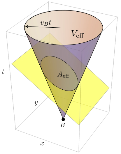
where is the dominant error per two-qubit entangling gate and the effective circuit volume. For systems without conservation laws, the effective volume is the number of entangling two-qubit gates that contribute to the expectation value . Note that depends on the specific observable . The corresponding computational cost with tensor network contraction will be exponential in some “effective area” of an appropriate “cut” of the effective volume , that is,
| (3) |
for some constant 222A more formal definition of the computational cost of a tensor network contraction shows that it is exponential in the so called treewidth of the corresponding tensor network.. (See Fig. 1 for a cartoon of and for a single qubit Pauli operator.) Therefore, we typically expect a tradeoff between the desirable high signal-to-noise ratio, and the coveted high classical computational cost (high .
In Sec. II we detail this framework in the context of RCS, where it arises more naturally. In Sec. III we summarize how this framework was extended to local observables in Ref. [6]. In Sec. IV we apply this framework to the Floquet circuit unitary of Ref. [7], and present simulations of this experiment with a cost of less than one second per data point using one GPU, employing generic methods.
II Random Circuit Sampling
Random quantum circuit sampling (RCS) is an experiment designed to benchmark both the achievable equivalent computational cost and the full system fidelity [1, 2, 5]. In this case the quantum circuit is chosen at random from an ensemble of quantum gates designed to maximize the spread of quantum correlations and the equivalent classical computational cost. Not coincidentally, this experiment is also particularly sensitive to noise.
In the presence of noise, the experimental value of an observable for a random circuit is
| (4) |
where is the density matrix of a noisy quantum state, is the number of qubits and is the fidelity of the quantum circuit. The fidelity can be approximated by
| (5) |
where is the circuit volume, the number of entangling two-qubit gates, and is the dominant error per gate.
There is a statistical error when measuring an observable , and we require . For a traceless observable , this puts a bound on the circuit volume
| (6) |
The corresponding classical computational cost is estimated by benchmarking an equivalent classical sampling of bitstrings such that , using the best classical algorithms available.
Standard full wave–function quantum circuit simulation algorithms store a direct representation of the full wave function where gates are applied. Therefore, despite significant recent improvements, their cost becomes prohibitive for simulating current quantum processors with around 50 qubits or more. Similarly, standard full wave-function tensor network algorithms, such as matrix product states (MPS) or 2D tensor networks, attempt to find a more efficient representation of the full wave–function when there is only limited entanglement, but they also become prohibitively expensive as the amount of entanglement in the quantum state grows.
Recent research has shown that classical tensor contraction algorithms are the most performant for the most complex recent quantum computation experiments. Tensor contraction algorithms are a generalization of quantum circuit simulation algorithms where each gate is interpreted as a tensor with indices connecting to neighboring gates. They were first implemented precisely to benchmark the classical computational cost of random circuit sampling [1, 2, 5].
For simplicity, consider a unitary circuit acting over time on a square -qubit array. The cost of tensor contraction scales like,
| (7) |
where is the area of a cut of the circuit volume [64]. For short evolution times and the cost is exponential in the maximum amount of entanglement generated by the circuit. The coefficient depends on the entangling power of the gate used. For instance, for iSWAP gates, while for CZ gates [39], determined by the Schmidt coefficients of the gate.
Therefore, we arrive at the following intuitive conclusion: for a fixed gate error , the feasibility or fidelity of the experiment decreases exponentially with the circuit volume, while the corresponding classical computational cost increases exponentially with the area of a cut of the circuit volume. The RCS experiment reported in Ref. [5] has an estimated contraction cost larger than [65] and fidelity of for the hardest circuits. The average error per iSWAP-like entangling gate was , and the (effective) volume was 702 gates. The estimated classical simulation time is 47.2 years if using the Frontier supercomputer, the only exascale supercomputer in the TOP500 list.
III Information scrambling with local operators
The relationship between gate error, the fidelity of an observable, and the corresponding computational cost, has also been analyzed recently in the context of quantum information scrambling 333Understanding how quantum information scrambles is essential to understanding a number of physical phenomena, such as the fast-scrambling conjecture for black holes, non-Fermi liquid behaviors, and many-body localization. Ref. [6] also provides a basis for designing near term quantum algorithms that would benefit from efficient exploration of the Hilbert space. with out-of-time-correlator (OTOC) measurements Ref. [6]. Quantum information scrambling can be seen as a “butterfly effect”, in which a small change in one location can quickly grow into a large change over time. More precisely, the disturbance is implemented as an initially local operator (the “butterfly operator”) , typically a Pauli operator acting on one of the qubits (the ”butterfly qubit”). Ref. [6] investigated the dynamic process in which the butterfly operator evolves under a random quantum circuit as , where is the inverse of . The information scrambling of this process is studied with an OTOC measurement where is another Pauli operator on a different qubit. The OTOC observable is encoded in the Pauli expectation value of an ancilla qubit “a” (see Ref. [6] for details).
The observable considered in Ref. [6] averaged over random circuits subject to experimental noise can be written in the first approximation as,
| (8) |
where is an effective fidelity 444See Ref. [6] for better approximations that take into account experimental bias of the outcome measurements and details of the propagation of errors for specific circuits.. The effective fidelity decays exponentially with the dominant error per two-qubit entangling gate and the effective circuit volume as
| (9) |
The effective volume is the number of entangling gates that contribute to the expectation value . In other words, removing any gate from would result in a relevant finite error in the reduced value of the observable , i.e. . Equation (8) offers a way to perform error mitigation by estimating the effective fidelity so that,
| (10) |
A single-qubit butterfly operator evolved with a circuit unitary is transformed into which has support on multiple qubits. This transformation proceeds via operator spreading: every time an entangling gate is applied to a pair of qubits crossing the boundary of the support increases with some probability . One might expect that under operator spreading is the subset of gates within the respective light cone of . However, this corresponds only to the case of , realized for example by a random circuit with iSWAP entangling gates. In generic random circuits the probability of spreading between two qubits is . The boundary of the support of remains relatively sharp, spreading at a (butterfly) velocity of , where is the light cone velocity. Reference [6] shows that, as an example, the butterfly velocity for random circuits is indeed less than the butterfly velocity of iSWAP random circuits. The butterfly velocity determines the size of the effective volume,
| (11) |
up to a factor of order one. In a noisy device only the noise channels associated with entangling gates within contribute to the measurement outcome which is reflected in Eqs. (8) and (9).
We note that the experiment reported in Ref. [6] can not be simulated by standard full wave function simulation algorithms, including full wave function matrix product states (MPS) or 2D tensor networks (iso-TNS). Indeed, in these circuits the entanglement spreads fast, and the entanglement entropy between two equal halves of the quantum system saturates quickly. The bond dimension required for a full wave function tensor network simulation for the circuits used in Ref. [6] would be , see App. A.
Nevertheless, as explained above, these are not the most efficient simulation algorithms. Tensor network contraction can be adapted to the problem of estimating the value of an observable, such as . Specifically, we can perform a tensor contraction where some output indices corresponding to some qubits are left “open”, i.e., they are not assigned to the value of a given output bitstring. The corresponding contraction produces a vector which encodes all the corresponding amplitudes for all possible assignments of the corresponding bits. The cost of a tensor network contraction with a relatively small number of open qubits is not much higher than a contraction with all “closed” or assigned qubits. Furthermore, it can be seen that the value of a local observable is independent of the value assigned to indices outside a relatively small neighborhood that contains the observable, see Ref. [6].
To accurately estimate the cost of an observable for a given circuit simulation, it is critical to note that the required tensor network only needs to contain the quantum gates within the effective volume. Therefore, the cost will be exponential in some “effective area” of an appropriate “cut” of the effective volume,
as in Eq. (7) 555More formally, the cost will be exponential in the treewidth of the line graph of the tensor network corresponding to the quantum circuit contained within the effective volume , see Fig. 1. Note that we assume as before that the circuit acts in a two dimensional array of qubits. We also have
| (12) |
with Butterfly velocity . For a long one dimensional array of qubits . Note the difference between Eqs. (3) and (12) is due to locality of operators and whereas in Eqs. (3) the measured operator has support on all qubits.
We arrive at a conclusion similar to the one for random circuit sampling. Namely, an experiment in a quantum processor is fundamentally limited by the exponential decrease in fidelity with the effective quantum volume, while the equivalent classical computational cost increases exponentially with an effective area . In other words, while experimentally we would like a small effective volume to obtain a good experimental signal-to-noise ratio, this consideration will limit the corresponding achievable computational complexity. We emphasize that the exponent in the fidelity, , and the exponent in the cost , have different scaling, see Eqs. (11) and (12).
The OTOC experiment reported in Ref. [6] had an effective fidelity , with an effective volume (light cone of iSWAPs) of 251 gates for the circuit size where the error mitigated signal-to-noise ratio was 1. The contraction cost was . The largest experiment reported in that reference, with a smaller signal-to-noise ratio, had an effective fidelity , with an effective volume of iSWAP gates and a contraction cost . The average error per iSWAP gate was .
As discussed above the cost estimated in Eq. (12) corresponds to a general purpose tensor network contraction algorithm. However, often there exist model-specific approximate methods that use analytical insights to significantly reduce the computational cost, such as stabilizer based algorithms exploiting the Clifford group, or mappings to free fermions. Another instructive example was discussed in Ref. [6], where the value of OTOC averaged over instances of random circuits can be predicted at a fraction of the computational cost, specifically using a mapping onto a classical Markov chain. At the same time, there are no known efficient classical methods to compute the value of OTOC for a specific instance of a random circuit, and tensor contraction remains the best performing algorithm. The effective circuit volume of such a simulation is estimated from the precision needed to resolve the circuit-specific variation of OTOC. Therefore, the variance of OTOC determines the conditions on the above task for a quantum simulation to surpass classical supercomputers for all known classical algorithms.
IV Time ordered observables
The above considerations apply to experiments in quantum processors more generally. We consider for simplicity experiments estimating a (time ordered) expectation value of a string of Pauli operators with support in qubits. Under appropriate experimental conditions we expect, as in Eq. (8),
| (13) |
where is the effective fidelity of the experimental measurement and is the corresponding effective circuit volume, see Eq. (9).
We first consider the evolution of a local operator in the generic case when the quantum state becomes chaotic (or ergodic) and the information scrambling takes hold. In this case decays very rapidly to 0 on a time scale given by the inverse of the butterfly velocity . The corresponding effective volume and the cost will be limited by statistical error or by the effective fidelity, see App. B.
A more interesting case is when the transition to chaos is preceded at early stages by a so-called prethermalization regime where can decay slowly to 0. One example is given by Floquet circuits with layers of control-phase gates and single qubit rotations with not too large angles. This typically corresponds to a Floquet transverse field Ising model, where the cycle unitary and the corresponding Floquet Hamiltonian posses an Ising symmetry leading to a spontaneous symmetry broken phase away from the critical point. This generic model has been used in experimental simulations exploring quantum many-body phenomena, such as time crystals [33, 31], quantum scars [32], Majorana edge modes [34] and dissipative bath engineering [37].
A recent experiment with this system consists of ZZ rotations and X rotations with the same angle for all the qubits [7]. Explicitly, the Floquet circuit is
| (14) |
where denotes nearest neighbors. The initial condition, all spins up, corresponds, with small angles , to a system deeply in the ferromagnetic symmetry broken phase. There the magnetization is large and the correlators decay quickly with distance (short correlation length).
The experiment [7] uses an error mitigation technique that similarly to the one explained in Sec. III, relies on Eq. (10). The effective fidelity is estimated experimentally by adding errors in a controlled way, which is related to increasing the component error , and fitting the corresponding exponential decay of .
IV.1 Local time-ordered observable
In some of the experiments reported in Ref. [7], including the ones corresponding to the largest circuits, the measurement consists of a single Pauli operator as a function of . One way to estimate the effective circuit volume for a given observable from experimental data is by using the corresponding effective fidelity. This can be determined from the ratio of unmitigated and mitigated data points in the experimental data shown in Fig. 4b of Ref. [7], see also Fig. 3. The data shows for the qubit labeled 62 with 20 steps (60 layers of two-qubit gates) of the Floquet circuit of Eq. (14). The light cone covers all 127 qubits in Fig. 2. For the data points corresponding to we obtain
| (15) |
and lager values for . Using the average error rate per entangling gate reported in Ref. [7] we obtain an estimate of the effective circuit volume of gates. Note that is substantially smaller than the 2880 two-qubit entangling gates in the circuit. The fidelity of a circuit for this effective volume would be . This suggests that the cost of an optimal tensor network contraction for such a local observable must be significantly lower than simulating state evolution subject to all of the gates applied in the experiment.
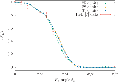
This suggests that a simulation of a smaller circuit could reproduce the observed data points. Indeed in Fig. 4 we compare experimental data points extracted from Fig. 4b of Ref. [7] to numerical simulations with a smaller number of qubits . The difference between numerical simulations with 28 and 31 qubits is much smaller than the 1-sigma error bars of the experiment for all values of . This good agreement, the clear convergence seen at lower depth (see App. C.3), and related numerics in App. C.2, suggest that the numerical simulation is more accurate than the experiment. See also App. C.3 for the convergence of the magnetization in a smaller experiment, where it again does not require the simulation of the full light cone. Simulations with 25 qubits or fewer show good convergence for , corresponding to the small correlation length deeply in the ferromagnetic symmetry broken phase. We also see a good agreement for large , corresponding to the ergodic case. Each point per value is obtained in 0.8 seconds on an A100 GPU using the open source simulator qsim [70, 71, 72] for , and 6.9 seconds per for 666In the process of finishing this paper, another paper appeared with a different method that performs the same simulations [75]. Our results and the results in this reference agree, except for large values reported in Fig. 3b in Ref. [75], Fig. 4b in Ref. [7] and Figs. 4 and 12 here. We note that Ref. [75] overestimates the value of in the neighborhood of . As explained in App. B this value of is in the ergodic regime, and is 0, which is also what we obtain by direct numerical simulation..
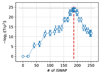
We now attempt to reduce the cost of the numerical simulations by optimizing the contraction ordering of the circuits simulated over qubits, see Fig. 3, and discarding every gate outside of the light cone of propagated backwards. We look at both an “open” contraction, with all output indices of the circuit uncontracted, and a “closed” contraction, where a bit string is specified at the output of the circuit, typically leading to a lower cost, although resulting in the computation of a single amplitude. The optimized cost of the open contraction is , while for the closed contraction we get [65]. This is to be compared to (560 two-qubit gates over 28 qubits) for a full state vector time evolution, similar to qsim’s numerical simulations. The similarity between the three costs, which are exponential in , is not surprising, given that this circuit is in the high-depth regime, i.e., the depth of the circuit is larger than the width of the lattice of qubits simulated.
The above results suggest that the spontaneously broken phase, characterized by non-zero quasi-static magnetization and finite correlation length, persists for large values of , corresponding to the regime of pre-thermalization, see Sec. B.2 for details. In this case the state vector of the system has overlap with the uniformly polarized initial state and at the same time contains excitations that may not necessarily contribute to the local magnetization. Most of the components of the state vector that do contribute to the magnetization have correlation length smaller than the linear dimensions of the qubit systems we considered in our simulations.
We emphasize that the situation here is remarkably different from the out-of-time-order observable explained in Sec. III. Indeed, the effective volume of an out-of-time-order correlator between distant ancilla and butterfly qubits can be an open cone with a diameter growing with the butterly velocity. Consequently, the cost of tensor network contraction grows exponentially with the square of the distance between the ancilla and butterfly qubits, while the effective fidelity decreases exponentially with the cube of this distance. In contrast, the effective volume of a local observable of a physical system with a given correlation length is a cylinder with a diameter proportional to this length. In this case the cost of tensor network contraction grows exponentially with the square of the correlation length, while the effective fidelity decreases exponentially with the cube of the correlation length.
IV.2 Non-local observable

Reference [7] also uses non-local Pauli observables of support extending up to 17 qubits. Noting that circuits with are Clifford circuits, these observables are chosen by evolving a single qubit Pauli at time zero to obtain a high weight stabilizer at the final depth. This immediately implies that the effective volume at is an inverted cone between the high weight stabilizer at the final depth and the single qubit chosen for the stabilizer at the initial time. This effective volume is smaller than the light cone, which grows from the final non-local observable support to cover a larger number of qubits at the initial time. This again is consistent with the relatively high effective fidelity observed in Ref. [7]. For example, for the hardest non-local observable presented in Ref. [7] Fig. 4a the effective fidelity goes from up to , with an effective volume . We therefore expect, as before, that the correct result can be well approximated with simulations using less qubits than the light cone.
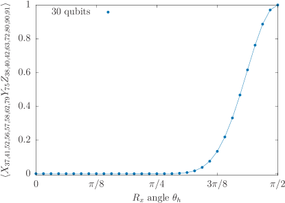
Figure 5 shows the expectation value as a function of for an observable composed of 17 Pauli operators, see Ref. [7] Fig. 4a, after 5 Floquet steps with Eq. (14) followed by single-qubit rotations. The numerical simulations agree with the experimental value from Ref. [7] Fig. 4a except for one point at close to . On similar simulations where we can compare with exact results, such as Figs. 10 and 11 in App. C, we test that again we do not need to simulate the full light cone. Furthermore, we note that in the same cases the experimental value in Ref. [7] underestimates the exact value when it is close to 0. Therefore, the numerics are likely more accurate than the experiment for the point where they do not agree. Each point is obtained in less than one second per value on an A100 GPU using the open source simulator qsim [70, 71, 72].
Similar to Section IV.1, we optimize tensor network
contraction costs for the circuit simulated with qsim with and
discarding gates laying outside of the observable’s light cone. For the open
contraction we get a cost of , while for the closed contraction we
get . This is to be compared to for the full state
vector time evolution (161 two-qubit gates over 30 qubits), similar to qsim’s
numerical simulations. We now see a reduction in the contraction cost from a
state vector time evolution to an optimized open contraction (both exponential
in ), which is further reduced substantially by a factor of
for the closed contraction. While the closed contraction results in only one
amplitude per computation, one can use it as a primitive to sample bit strings
from the circuit with a method such as that introduced in
Ref. [74] at a cost per sample that grows linearly in the
number of gates and in the closed contraction cost. Samples can then be used
to estimate the expectation value of the observables studied. These numerical
simulation costs are to be compared with those of random circuit sampling
experiments. In the case of Ref. [5], the hardest circuits
are estimated to require a cost larger than .
In summary, a small effective quantum volume is the main reason why experiments
of Ref. [7] can be simulated on a classical computer. In
principle, a larger volume may be obtained by increasing the depth of the
circuits, hence increasing the spread of the observables, or by changing the
design of the circuits considered. On the one hand, without increasing the gate
fidelity, a potentially larger effective quantum volume will result in an
exponentially suppressed signal to noise ratio, which would make an experiment
impractical. On the other hand, as in the case of the prethermalized
ferromagnetic states of Ref. [7], the short correlation
length results in a small effective circuit volume, hence reducing the
classical computational cost. In the end, an increased gate fidelity and a
careful design of the experiments is of utmost importance to reach the
beyond-classical regime.
Related works: At the time of and after writing this manuscript, other groups [75, 76, 77, 78, 79] have developed approximate simulations of the experiments of Ref. [7] using different numerical techniques. For instance, Refs. [75] and [79] use an approximate evolution of the wave function, which is encoded as a compressed tensor network that matches the connectivity of the experimental device. Other approaches are based on the approximate Heisenberg evolution of the observable [76, 77, 78, 79]. These approximate evolutions are either carried out on a truncated basis of Pauli strings [76], on a compressed matrix product operator representation of the operator [77], or on a compressed two-dimensional tensor network that matches the connectivity of the device [78]. Interestingly, Ref. [76] also provides a hybrid method in which both the operator and the wave function are represented with respective tensor networks with device-like connectivity, each of which is partially evolved.
Note that our approximation method is substantially different than the aforementioned approaches. More precisely, we introduce and exploit the concept of an effective quantum volume to reduce the classical computational cost. Indeed, in the experiments of Ref. [7], the effective quantum volume is smaller than the maximum volume that can be classically simulated. Interestingly, the success of the approximate methods of Refs. [75, 76, 77, 78, 79] can be reduced to small quantum volume for the experiments of Ref. [7] First, the same slow spread of the observable under a Heisenberg evolution that gives rise to this small effective quantum volume is responsible for the slow spread of correlations in the evolved operator. This, in turn, allows the Heisenberg evolution methods studied by Refs. [76, 77, 78, 79] to approximate well the results of the experiments of Ref. [7] with low computational resources. In addition, the sparsity of the qubit layout of these experiments, which is key to the success of the tensor network methods mentioned above [75, 76, 77, 78, 79], contributes to the slow spread of the observables which is central to our work.
V Conclusion
The computational cost of a local observable simulation can be upper bounded by the effective circuit volume, that is, the minimal number of gates needed to calculate this observable with a given precision. As was shown in Ref. [6], the effective volume can become prohibitively large for classical simulations in the task of measuring OTOC for a random circuit converging to the ergodic regime. The classical computational cost increases as the dynamics approaches chaos, yet at the same time the value of all local observables decreases even in the noise free case, and therefore the precision required for a reliable measurement increases.
In a realistic device gates have an error , and often entangling gates have the highest error compared to other operations. This further decreases the signal-to-noise ratio. Consequently, noise also reduces the effective volume, and the achievable classical computational cost that is feasible with a given precision. Nevertheless, for sufficiently low noise, the finite achievable effective volume would have a prohibitively high computational cost. Ref. [6] is an example of a quantum circuit experiment that explores this trade off.
We would like to emphasize that the effective circuit volume strongly depends on the specific observable. The effective volume is bounded in time and space by the correlation time and length of the states that contribute to the observable. For example, the prethermalized ferromagnetic states considered above in the context of a Floquet transverse field Ising model [7] are characterized by static magnetization that at first sight appears to be advantageous for the signal to computational cost trade-off. However, such ordered states are characterized by a short correlation length that limits the effective circuit volume and corresponding computational cost even at long simulation times. In the ergodic regime, the decay of time-ordered correlators (TOC) is characterized by very short correlation time, that also limits the effective volume and computational cost.
Summarizing the discussion above, in the quest for a beyond-classical regime in noisy quantum processors, one has to choose observables carefully. The same applies for comparing quantum simulations with brute force classical methods. To illustrate this point, we presented numerical simulations of a Floquet circuit unitary experiment [7], using generic methods, with a computational cost of less than one second per data point on one GPU.
We note in passing that the relationship between the effective circuit volume and the noise parameters can be more complicated than the scaling used above. Examples include systems that map on free or weakly-interacting fermions and systems with conserved number of particles. However, this does not change the fact that increasing noise reduces the effective circuit volume and the magnitude of the expectation value Eq. (13), therefore reducing the cost of classical simulation.
Acknowledgements.
We thank Orion Martin for writing the colabs that exemplify the simulations of Figs. 4 and 5. We thank the Google Quantum AI team for numerous fruitful discussions. S. Mandrà is partially supported by the Prime Contract No. 80ARC020D0010 with the NASA Ames Research Center and acknowledges funding from DARPA under IAA 8839.Appendix A Entanglement estimation for the circuits in Ref. [6]
Reference. [5] shows that the required bond dimension for standard tensor network simulations of random circuits can be bounded by computing the averaged reduced purity . These circuits are similar to the ones used in Ref. [6]. Furthermore, the average reduced purity is the same for an equivalent ensemble of Clifford circuits (that is, using Clifford single-qubit rotations only). More precisely, we can bound the required bond dimension as [5]
| (16) |
where is the target fidelity. Figure 6 shows the reduced purity for random OTOC Clifford circuits with a total number of entangling gates, the largest OTOC circuits in Ref. [6]. As expected, the lower bound for grows untill it reaches its maximum when the butterfly operator is applied. At its maximum, almost reaches its saturation value, meaning that there is no gain in using MPS or other standard tensor network simulations for the largest circuits in Ref. [6].
Appendix B Chaotic dynamics with local time-ordered observable
B.1 2D lattice
Many quantum simulation tasks in quantum chemistry, material science, and physics require measurement of an expectation value of a local operator with respect to some initial product wave function which can be prepared easily. Quantum dynamics in absence of an extensive number of conservation laws exhibit quantum chaos at long time scale. The long time asymptotic of a local observable scales as with the total Hilbert space of the -qubit system. Convergence to this limit is determined by the microscopic details of the evolution operator and the locality/connectivity of the qubit array. Nonetheless, the scaling with circuit depth can be deduced from the following qualitative analysis of operator spreading. For example, consider a single qubit Pauli located at the origin of a square 2D grid, evolving under without conserved quantities. In the Heisenberg picture can described using an expansion into Pauli strings,
| (17) |
with , and we assumed a two-dimensional square grid of qubits labeled by pairs of indexes . Note that the coefficients are normalized as .
A single qubit Pauli operator subject to a two-qubit entangling gate is transformed into a superposition of two-qubit Pauli strings. Subsequent application of two-qubit gates increases the size of the Pauli strings in the superposition. This gives rise to operator spreading. It proceeds in real space such that at a given time all Paulis located sufficiently far from (at the origin) equal the identity, . Such dynamics can be characterized by a spatial distribution of the boundary of the support of ,
| (18) |
where for a given Pauli string , is the distance from the origin of the farthest non-identity Pauli . In the absence of conservation laws the operator spreading is ballistic. In these cases the distribution is sharply peaked around the boundary of the support of the operator (a front). Then the time dependent size of the operator can be described by the average,
| (19) |
Because of the approach to quantum chaos for the coefficients are uniformly random such that the Paulis have equal probability with absolute values where is the number of qubits within the support. Ballistic propagation is characterized by a butterfly velocity, .
Consider an initial state polarized along the -axis and without loss of generality. In the expansion (17) only Pauli strings consisting of and operators contribute non-zero values to the expectation value . In this case
| (20) |
The latter estimate corresponds to the fact that the sum is over terms of random signs. Including the ballistic spreading of the operator we obtain,
| (21) |
Note that the expectation value decays with a characteristics time scale . Using similar arguments we obtain the scaling of the correlation functions. For example the equal time two-point correlator is
| (22) |
where, , and, , is the area of intersection of the supports of the operators and , and is the sum of the support areas. The form of the function is quite involved. Similarly to the case of a single observable (20) the leading factors in the dependence of on contain and the dependence on contains the factor .
The effective computational volume is given by the gates within a cone in three-dimensional space-time. The base of the cone has area and is formed by qubits inside the support of . The height of the cone corresponds to the circuit depth . The circuit volume increases as .
We note that the expectation value and the correlator decay rapidly on the time scale . Therefore the circuit depth and the respective circuit volume are limited by the desired precision and the gate error via Eq. (6).
In the presence of noise the observable equals,
| (23) |
Using the relation between fidelity and the circuit volume , the depth of feasible quantum simulation is limited by characteristic time that is the solution of the equation ,
| (24) |
In the case of zero gate error
In the case of large gate errors the decay of the observable is determined by the decay of the fidelity
| (25) |
The cost of tensor contraction, Eq. 3, depends on the butterfly velocity.
| (26) |
where depends on the type of the gate.
B.2 1D and low degree 2D
It is instructive to also report the respective results for one-dimensional system, a local observable in the interior of a long chain of qubits will scale as,
| (27) |
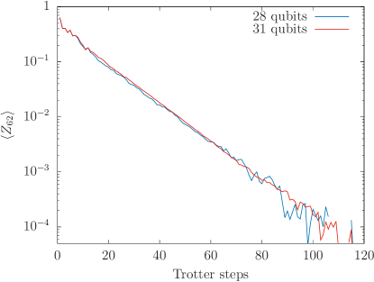
Note that in the case of experiment reported in Ref. [7] the qubit lattice is substantially different from square lattice: the number of nearest neighbors is for two qubits, for 89 qubits, and for 36 qubits. In other words this lattice is closer to one-dimension than to the square lattice.
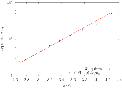
Figure 7 shows the exponential decay of the magnetization for for the lattice in Ref. [7], in agreement with Eq. (27). Figure 8 shows the exponential scaling of the magnetization steps-to-decay as a function of . This is expected scaling for prethermalization [80]. For small , deep in the prethermalization phase, the number of steps to decay becomes very long because large phases of gates make it hard to flip the magnetizations of individual qubits.
Appendix C Additional numerical simulations
C.1 Simulations for other figures in Ref. [7]
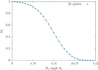
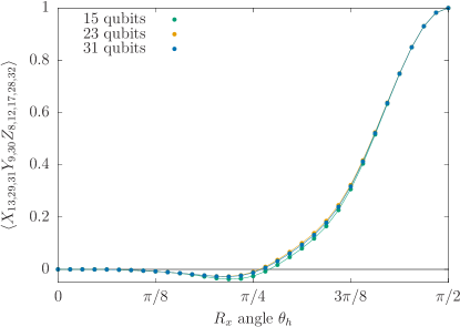
For completeness, we include numerical simulations for the circuits in Figs. 3a, 3b and 3c of Ref. [7]. In all cases the numerical simulations agree with the experimental results presented there. Figure 9 shows the average magnetization as a function of for the 28 qubits of Fig. 3 after five steps of the Floquet circuit of Eq. (14). Figures 10 and 11 show the numerical simulation of an observable with 10 and 17 Pauli operators respectively, after five Floquet steps. In each case the observable corresponds to a stabilizer of the Clifford circuit obtained from the evolution of an initial single stabilizer.
Figure 10 compares simulations with 15, 23 and 31 qubits for the 10 Pauli operator measured in Ref. [7] Fig. 3b. Note that there is a small difference between 15 and 23 qubits, although this difference is smaller than the experimental error bars in Ref. [7]. Nevertheless, there is good agreement between the simulations with 23 and 31 qubits. The light cone is 37 qubits, indicating that simulations of the smaller effective volume are sufficient to obtain a good estimation of the observable.
C.2 Closed vs. open loops
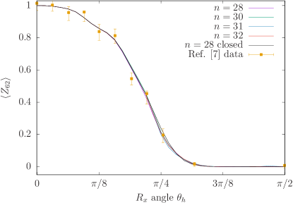
Figure 12 shows numerical simulations for of the qubit labelled 62 in Fig. 3, with 20 steps of the Floquet circuit of Eq. (14). We compare numerical simulations with close loops, see Fig. 3, and simulations with up to qubits without closing the corresponding loops (open boundary). We see a good agreement for the estimation expectation value of in all cases.
C.3 Convergence of at 5 steps
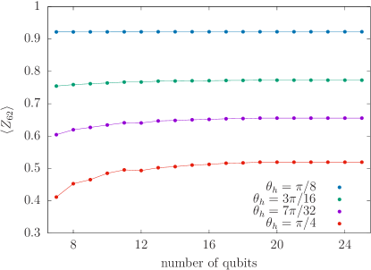
Figure 13 shows numerical estimations of at the qubit labeled 62 in Fig. 3 with the Floquet circuit of Eq. (14) and 5 steps. We show results for a growing number of qubits, between 7 and 25, the size of the light cone. Smaller values of have higher magnetization, and converge to the correct result with a smaller number of qubits. As explained in Sec. IV.1, the reason is that this corresponds to prethermalized ferromagnetic states characterized by a short correlation length that limits the effective circuit volume. Larger values presumably correspond to states with larger correlation length. Nevertheless, the magnetization converges to the correct value with less qubits than the light cone even for the larger . Approximately after this value the state becomes ergodic and the magnetization converges exponentially to 0, see App. B.
References
- Boixo et al. [2018] S. Boixo, S. V. Isakov, V. N. Smelyanskiy, R. Babbush, N. Ding, Z. Jiang, M. J. Bremner, J. M. Martinis, and H. Neven, Characterizing quantum supremacy in near-term devices, Nature Physics 14, 595 (2018).
- Arute et al. [2019] F. Arute, K. Arya, R. Babbush, D. Bacon, J. C. Bardin, R. Barends, R. Biswas, S. Boixo, F. G. Brandao, D. A. Buell, et al., Quantum supremacy using a programmable superconducting processor, Nature 574, 505 (2019).
- Wu et al. [2021] Y. Wu, W.-S. Bao, S. Cao, F. Chen, M.-C. Chen, X. Chen, T.-H. Chung, H. Deng, Y. Du, D. Fan, M. Gong, C. Guo, C. Guo, S. Guo, L. Han, L. Hong, H.-L. Huang, Y.-H. Huo, L. Li, N. Li, S. Li, Y. Li, F. Liang, C. Lin, J. Lin, H. Qian, D. Qiao, H. Rong, H. Su, L. Sun, L. Wang, S. Wang, D. Wu, Y. Xu, K. Yan, W. Yang, Y. Yang, Y. Ye, J. Yin, C. Ying, J. Yu, C. Zha, C. Zhang, H. Zhang, K. Zhang, Y. Zhang, H. Zhao, Y. Zhao, L. Zhou, Q. Zhu, C.-Y. Lu, C.-Z. Peng, X. Zhu, and J.-W. Pan, Strong quantum computational advantage using a superconducting quantum processor, Physical Review Letters 127, 180501 (2021).
- Zhu et al. [2022] Q. Zhu, S. Cao, F. Chen, M.-C. Chen, X. Chen, T.-H. Chung, H. Deng, Y. Du, D. Fan, M. Gong, C. Guo, C. Guo, S. Guo, L. Han, L. Hong, H.-L. Huang, Y.-H. Huo, L. Li, N. Li, S. Li, Y. Li, F. Liang, C. Lin, J. Lin, H. Qian, D. Qiao, H. Rong, H. Su, L. Sun, L. Wang, S. Wang, D. Wu, Y. Wu, Y. Xu, K. Yan, W. Yang, Y. Yang, Y. Ye, J. Yin, C. Ying, J. Yu, C. Zha, C. Zhang, H. Zhang, K. Zhang, Y. Zhang, H. Zhao, Y. Zhao, L. Zhou, C.-Y. Lu, C.-Z. Peng, X. Zhu, and J.-W. Pan, Quantum computational advantage via 60-qubit 24-cycle random circuit sampling, Science Bulletin 67, 240 (2022).
- Morvan et al. [2023] A. Morvan, B. Villalonga, X. Mi, S. Mandrà, A. Bengtsson, P. Klimov, Z. Chen, S. Hong, C. Erickson, I. Drozdov, et al., Phase transition in random circuit sampling, arXiv preprint arXiv:2304.11119 (2023).
- Mi et al. [2021] X. Mi, P. Roushan, C. Quintana, S. Mandra, J. Marshall, C. Neill, F. Arute, K. Arya, J. Atalaya, R. Babbush, et al., Information scrambling in quantum circuits, Science 374, 1479 (2021).
- Kim et al. [2023] Y. Kim, A. Eddins, S. Anand, K. X. Wei, E. Van Den Berg, S. Rosenblatt, H. Nayfeh, Y. Wu, M. Zaletel, K. Temme, et al., Evidence for the utility of quantum computing before fault tolerance, Nature 618, 500 (2023).
- Feynman [2018] R. P. Feynman, Simulating physics with computers, in Feynman and computation (CRC Press, 2018) pp. 133–153.
- Shor [1995] P. W. Shor, Scheme for reducing decoherence in quantum computer memory, Physical review A 52, R2493 (1995).
- Gottesman [1997] D. Gottesman, Stabilizer codes and quantum error correction (California Institute of Technology, 1997).
- Knill et al. [1998] E. Knill, R. Laflamme, and W. H. Zurek, Resilient quantum computation, Science 279, 342 (1998).
- Kitaev [2003] A. Y. Kitaev, Fault-tolerant quantum computation by anyons, Annals of physics 303, 2 (2003).
- Dennis et al. [2002] E. Dennis, A. Kitaev, A. Landahl, and J. Preskill, Topological quantum memory, Journal of Mathematical Physics 43, 4452 (2002).
- Raussendorf and Harrington [2007] R. Raussendorf and J. Harrington, Fault-tolerant quantum computation with high threshold in two dimensions, Physical review letters 98, 190504 (2007).
- Fowler et al. [2012] A. G. Fowler, M. Mariantoni, J. M. Martinis, and A. N. Cleland, Surface codes: Towards practical large-scale quantum computation, Physical Review A 86, 032324 (2012).
- Satzinger et al. [2021] K. Satzinger, Y.-J. Liu, A. Smith, C. Knapp, M. Newman, C. Jones, Z. Chen, C. Quintana, X. Mi, A. Dunsworth, et al., Realizing topologically ordered states on a quantum processor, Science 374, 1237 (2021).
- Krinner et al. [2022] S. Krinner, N. Lacroix, A. Remm, A. Di Paolo, E. Genois, C. Leroux, C. Hellings, S. Lazar, F. Swiadek, J. Herrmann, et al., Realizing repeated quantum error correction in a distance-three surface code, Nature 605, 669 (2022).
- Zhao et al. [2022] Y. Zhao, Y. Ye, H.-L. Huang, Y. Zhang, D. Wu, H. Guan, Q. Zhu, Z. Wei, T. He, S. Cao, et al., Realization of an error-correcting surface code with superconducting qubits, Physical Review Letters 129, 030501 (2022).
- Acharya et al. [2023] R. Acharya, I. Aleiner, R. Allen, T. I. Andersen, M. Ansmann, F. Arute, K. Arya, A. Asfaw, J. Atalaya, R. Babbush, et al., Suppressing quantum errors by scaling a surface code logical qubit, Nature 614, 676 (2023).
- Shor [1994] P. W. Shor, Algorithms for quantum computation: discrete logarithms and factoring, in Proceedings 35th annual symposium on foundations of computer science (Ieee, 1994) pp. 124–134.
- Gidney and Ekerå [2021] C. Gidney and M. Ekerå, How to factor 2048 bit rsa integers in 8 hours using 20 million noisy qubits, Quantum 5, 433 (2021).
- Lloyd [1996] S. Lloyd, Universal quantum simulators, Science 273, 1073 (1996).
- Aspuru-Guzik et al. [2005] A. Aspuru-Guzik, A. D. Dutoi, P. J. Love, and M. Head-Gordon, Simulated quantum computation of molecular energies, Science 309, 1704 (2005).
- Quantum et al. [2020] G. A. Quantum, Collaborators*†, F. Arute, K. Arya, R. Babbush, D. Bacon, J. C. Bardin, R. Barends, S. Boixo, M. Broughton, B. B. Buckley, et al., Hartree-fock on a superconducting qubit quantum computer, Science 369, 1084 (2020).
- Huggins et al. [2022] W. J. Huggins, B. A. O’Gorman, N. C. Rubin, D. R. Reichman, R. Babbush, and J. Lee, Unbiasing fermionic quantum monte carlo with a quantum computer, Nature 603, 416 (2022).
- Goings et al. [2022] J. J. Goings, A. White, J. Lee, C. S. Tautermann, M. Degroote, C. Gidney, T. Shiozaki, R. Babbush, and N. C. Rubin, Reliably assessing the electronic structure of cytochrome p450 on today’s classical computers and tomorrow’s quantum computers, Proceedings of the National Academy of Sciences 119, e2203533119 (2022).
- Rubin et al. [2023] N. C. Rubin, D. W. Berry, F. D. Malone, A. F. White, T. Khattar, A. E. D. I. au2, S. Sicolo, M. Kühn, M. Kaicher, J. Lee, and R. Babbush, Fault-tolerant quantum simulation of materials using bloch orbitals (2023), arXiv:2302.05531 [quant-ph] .
- Huang et al. [2022] H.-Y. Huang, M. Broughton, J. Cotler, S. Chen, J. Li, M. Mohseni, H. Neven, R. Babbush, R. Kueng, J. Preskill, et al., Quantum advantage in learning from experiments, Science 376, 1182 (2022).
- Lloyd et al. [2016] S. Lloyd, S. Garnerone, and P. Zanardi, Quantum algorithms for topological and geometric analysis of data, Nature communications 7, 10138 (2016).
- Berry et al. [2022] D. W. Berry, Y. Su, C. Gyurik, R. King, J. Basso, A. D. T. Barba, A. Rajput, N. Wiebe, V. Dunjko, and R. Babbush, Quantifying quantum advantage in topological data analysis, arXiv preprint arXiv:2209.13581 (2022).
- Frey and Rachel [2022] P. Frey and S. Rachel, Realization of a discrete time crystal on 57 qubits of a quantum computer, Science Advances 8, eabm7652 (2022).
- Chen et al. [2022] I.-C. Chen, B. Burdick, Y. Yao, P. P. Orth, and T. Iadecola, Error-mitigated simulation of quantum many-body scars on quantum computers with pulse-level control, Physical Review Research 4, 043027 (2022).
- Mi et al. [2022a] X. Mi, M. Ippoliti, C. Quintana, A. Greene, Z. Chen, J. Gross, F. Arute, K. Arya, J. Atalaya, R. Babbush, et al., Time-crystalline eigenstate order on a quantum processor, Nature 601, 531 (2022a).
- Mi et al. [2022b] X. Mi, M. Sonner, M. Niu, K. Lee, B. Foxen, R. Acharya, I. Aleiner, T. Andersen, F. Arute, K. Arya, et al., Noise-resilient edge modes on a chain of superconducting qubits, Science 378, 785 (2022b).
- Morvan et al. [2022] A. Morvan, T. Andersen, X. Mi, C. Neill, A. Petukhov, K. Kechedzhi, D. Abanin, A. Michailidis, R. Acharya, F. Arute, et al., Formation of robust bound states of interacting microwave photons, Nature 612, 240 (2022).
- Andersen et al. [2023] T. Andersen, Y. Lensky, K. Kechedzhi, I. Drozdov, A. Bengtsson, S. Hong, A. Morvan, X. Mi, A. Opremcak, R. Acharya, et al., Non-abelian braiding of graph vertices in a superconducting processor, Nature , 1 (2023).
- Mi et al. [2023] X. Mi, A. A. Michailidis, S. Shabani, et al., Stable quantum-correlated many body states via engineered dissipation (2023), arXiv:2304.13878 [quant-ph] .
- Note [1] A circuit based quantum simulation of quantum information scrambling [6], which measures an expectation value of a local observable, has surpassed standard full wave function simulation algorithms, e.g., exact Schrodinger evolution and Matrix Product States (MPS). We note that this value can still be calculated with tensor network contraction [6].
- Markov et al. [2018] I. L. Markov, A. Fatima, S. V. Isakov, and S. Boixo, Quantum supremacy is both closer and farther than it appears, arXiv preprint arXiv:1807.10749 (2018).
- Bouland et al. [2019] A. Bouland, B. Fefferman, C. Nirkhe, and U. Vazirani, On the complexity and verification of quantum random circuit sampling, Nature Physics 15, 159 (2019).
- Zlokapa et al. [2020] A. Zlokapa, S. Boixo, and D. Lidar, Boundaries of quantum supremacy via random circuit sampling, arXiv preprint arXiv:2005.02464 (2020).
- Bouland et al. [2022] A. Bouland, B. Fefferman, Z. Landau, and Y. Liu, Noise and the frontier of quantum supremacy, in 2021 IEEE 62nd Annual Symposium on Foundations of Computer Science (FOCS) (IEEE, 2022) pp. 1308–1317.
- Kondo et al. [2022] Y. Kondo, R. Mori, and R. Movassagh, Quantum supremacy and hardness of estimating output probabilities of quantum circuits, in 2021 IEEE 62nd Annual Symposium on Foundations of Computer Science (FOCS) (IEEE, 2022) pp. 1296–1307.
- Aaronson and Hung [2023] S. Aaronson and S.-H. Hung, Certified randomness from quantum supremacy (2023), arXiv:2303.01625 [quant-ph] .
- Bassirian et al. [2021] R. Bassirian, A. Bouland, B. Fefferman, S. Gunn, and A. Tal, On certified randomness from quantum advantage experiments (2021), arXiv:2111.14846 [quant-ph] .
- Liu et al. [2021] Y. Liu, M. Otten, R. Bassirianjahromi, L. Jiang, and B. Fefferman, Benchmarking near-term quantum computers via random circuit sampling, arXiv preprint arXiv:2105.05232 (2021).
- Dalzell et al. [2022] A. M. Dalzell, N. Hunter-Jones, and F. G. S. L. Brandão, Random quantum circuits anticoncentrate in log depth, PRX Quantum 3, 010333 (2022).
- Gao et al. [2021] X. Gao, M. Kalinowski, C.-N. Chou, M. D. Lukin, B. Barak, and S. Choi, Limitations of linear cross-entropy as a measure for quantum advantage, arXiv preprint arXiv:2112.01657 (2021).
- Aharonov et al. [2022] D. Aharonov, X. Gao, Z. Landau, Y. Liu, and U. Vazirani, A polynomial-time classical algorithm for noisy random circuit sampling, arXiv preprint arXiv:2211.03999 (2022).
- De Raedt et al. [2019] H. De Raedt, F. Jin, D. Willsch, M. Willsch, N. Yoshioka, N. Ito, S. Yuan, and K. Michielsen, Massively parallel quantum computer simulator, eleven years later, Computer Physics Communications 237, 47 (2019).
- Pednault et al. [2017] E. Pednault, J. A. Gunnels, G. Nannicini, L. Horesh, T. Magerlein, E. Solomonik, and R. Wisnieff, Breaking the 49-qubit barrier in the simulation of quantum circuits, arXiv preprint arXiv:1710.05867 15 (2017).
- Markov and Shi [2008] I. L. Markov and Y. Shi, Simulating quantum computation by contracting tensor networks, SIAM Journal on Computing 38, 963 (2008).
- Boixo et al. [2017] S. Boixo, S. V. Isakov, V. N. Smelyanskiy, and H. Neven, Simulation of low-depth quantum circuits as complex undirected graphical models, arXiv preprint arXiv:1712.05384 (2017).
- Aaronson and Chen [2017] S. Aaronson and L. Chen, Complexity-theoretic foundations of quantum supremacy experiments, in 32nd Computational Complexity Conference (2017) p. 1.
- Chen et al. [2018] J. Chen, F. Zhang, C. Huang, M. Newman, and Y. Shi, Classical simulation of intermediate-size quantum circuits, arXiv preprint arXiv:1805.01450 (2018).
- Villalonga et al. [2019] B. Villalonga, S. Boixo, B. Nelson, C. Henze, E. Rieffel, R. Biswas, and S. Mandrà, A flexible high-performance simulator for verifying and benchmarking quantum circuits implemented on real hardware, npj Quantum Information 5, 86 (2019).
- Villalonga et al. [2020] B. Villalonga, D. Lyakh, S. Boixo, H. Neven, T. S. Humble, R. Biswas, E. G. Rieffel, A. Ho, and S. Mandrà , Establishing the quantum supremacy frontier with a 281 pflop/s simulation, Quantum Science and Technology 5, 034003 (2020).
- Gray and Kourtis [2021] J. Gray and S. Kourtis, Hyper-optimized tensor network contraction, Quantum 5, 410 (2021).
- Huang et al. [2020] C. Huang, F. Zhang, M. Newman, J. Cai, X. Gao, Z. Tian, J. Wu, H. Xu, H. Yu, B. Yuan, M. Szegedy, Y. Shi, and J. Chen, Classical simulation of quantum supremacy circuits, arXiv preprint arXiv:2005.06787 (2020).
- Kalachev et al. [2021] G. Kalachev, P. Panteleev, and M.-H. Yung, Multi-tensor contraction for xeb verification of quantum circuits, arXiv preprint arXiv:2108.05665 (2021).
- Villalonga et al. [2021] B. Villalonga, M. Y. Niu, L. Li, H. Neven, J. C. Platt, V. N. Smelyanskiy, and S. Boixo, Efficient approximation of experimental gaussian boson sampling, arXiv preprint arXiv:2109.11525 (2021).
- Pan et al. [2022] F. Pan, K. Chen, and P. Zhang, Solving the sampling problem of the sycamore quantum circuits, Physical Review Letters 129, 090502 (2022).
- Liu et al. [2022] Y. Liu, Y. Chen, C. Guo, J. Song, X. Shi, L. Gan, W. Wu, W. Wu, H. Fu, X. Liu, D. Chen, G. Yang, and J. Gao, Validating quantum-supremacy experiments with exact and fast tensor network contraction, arXiv preprint arXiv:2212.04749 (2022).
- Note [2] A more formal definition of the computational cost of a tensor network contraction shows that it is exponential in the so called treewidth of the corresponding tensor network.
- foo [a] To translate into FLOPs for single precision complex scalars one should multiply by a factor of .
- Note [3] Understanding how quantum information scrambles is essential to understanding a number of physical phenomena, such as the fast-scrambling conjecture for black holes, non-Fermi liquid behaviors, and many-body localization. Ref. [6] also provides a basis for designing near term quantum algorithms that would benefit from efficient exploration of the Hilbert space.
- Note [4] See Ref. [6] for better approximations that take into account experimental bias of the outcome measurements and details of the propagation of errors for specific circuits.
- Arute et al. [2020] F. Arute, K. Arya, R. Babbush, D. Bacon, J. C. Bardin, R. Barends, A. Bengtsson, S. Boixo, M. Broughton, B. B. Buckley, et al., Observation of separated dynamics of charge and spin in the fermi-hubbard model, arXiv preprint arXiv:2010.07965 (2020).
- Note [5] More formally, the cost will be exponential in the treewidth of the line graph of the tensor network corresponding to the quantum circuit contained within the effective volume .
- Quantum AI team and collaborators [2020] Quantum AI team and collaborators, qsim (2020), 10.5281/zenodo.4023103 .
- Isakov et al. [2021] S. V. Isakov, D. Kafri, O. Martin, C. V. Heidweiller, W. Mruczkiewicz, M. P. Harrigan, N. C. Rubin, R. Thomson, M. Broughton, K. Kissell, E. Peters, E. Gustafson, A. C. Y. Li, H. Lamm, G. Perdue, A. K. Ho, D. Strain, and S. Boixo, Simulations of quantum circuits with approximate noise using qsim and cirq (2021), arXiv:2111.02396 [quant-ph] .
- foo [b] The code used to simulate the model in equation (14) is attached to this arxiv submission. The code is also available online: https://github.com/quantumlib/Cirq/blob/master/examples/advanced/quantum_utility_sim_4a.ipynb and https://github.com/quantumlib/Cirq/blob/master/examples/advanced/quantum_utility_sim_4b.ipynb.
- Note [6] In the process of finishing this paper, another paper appeared with a different method that performs the same simulations [75]. Our results and the results in this reference agree, except for large values reported in Fig. 3b in Ref. [75], Fig. 4b in Ref. [7] and Figs. 4 and 12 here. We note that Ref. [75] overestimates the value of in the neighborhood of . As explained in App. B this value of is in the ergodic regime, and is 0, which is also what we obtain by direct numerical simulation.
- Bravyi et al. [2022] S. Bravyi, D. Gosset, and Y. Liu, How to simulate quantum measurement without computing marginals, Physical Review Letters 128, 220503 (2022).
- Tindall et al. [2023] J. Tindall, M. Fishman, M. Stoudenmire, and D. Sels, Efficient tensor network simulation of ibm’s kicked ising experiment (2023), arXiv:2306.14887 [quant-ph] .
- Begušić and Chan [2023] T. Begušić and G. K. Chan, Fast classical simulation of evidence for the utility of quantum computing before fault tolerance, arXiv preprint arXiv:2306.16372 (2023).
- Anand et al. [2023] S. Anand, K. Temme, A. Kandala, and M. Zaletel, Classical benchmarking of zero noise extrapolation beyond the exactly-verifiable regime, arXiv preprint arXiv:2306.17839 (2023).
- Liao et al. [2023] H.-J. Liao, K. Wang, Z.-S. Zhou, P. Zhang, and T. Xiang, Simulation of ibm’s kicked ising experiment with projected entangled pair operator, arXiv preprint arXiv:2308.03082 (2023).
- Patra et al. [2023] S. Patra, S. S. Jahromi, S. Singh, and R. Orús, Efficient tensor network simulation of ibm’s largest quantum processors, arXiv preprint arXiv:2309.15642 (2023).
- Abanin et al. [2015] D. A. Abanin, W. De Roeck, and F. m. c. Huveneers, Exponentially slow heating in periodically driven many-body systems, Phys. Rev. Lett. 115, 256803 (2015).