Disentangled Variational Auto-encoder Enhanced by Counterfactual Data for Debiasing Recommendation

Abstract

Recommender system always suffers from various recommendation biases, seriously hindering its development. In this light, a series of debias methods have been proposed in the recommender system, especially for two most common biases, i.e., popularity bias and amplified subjective bias. However, existing debias methods usually concentrate on correcting a single bias. Such single-functionality debiases neglect the bias-coupling issue in which the recommended items are collectively attributed to multiple biases. Besides, previous work cannot tackle the lacking supervised signals brought by sparse data, yet which has become a commonplace in the recommender system. In this work, we introduce a disentangled debias variational auto-encoder framework(DB-VAE) to address the single-functionality issue as well as a counterfactual data enhancement method to mitigate the adverse effect due to the data sparsity. In specific, DB-VAE first extracts two types of extreme items only affected by a single bias based on the collier theory, which are respectively employed to learn the latent representation of corresponding biases, thereby realizing the bias decoupling. In this way, the exact unbiased user representation can be learned by these decoupled bias representations. Furthermore, the data generation module employs Pearl’s framework to produce massive counterfactual data, making up the lacking supervised signals due to the sparse data. Extensive experiments on three real-world datasets demonstrate the effectiveness of our proposed model. Besides, the counterfactual data can further improve DB-VAE, especially on the dataset with low sparsity.

1 Introduction

Recommender system(RS) helps users find new items of personal preference from huge amounts of data, which is extensively employed in a myriad of on-the-fly applications, such as e-commerce[42, 8], social networks[22] and advertisement[13]. In realistic applications, the recommender system severely suffers from some widespread biases [41, 46, 43] (e.g., the popularity bias[46, 39] and the amplified subjective bias[36]), being incapable of accurately grasping the user’s personal preferences.

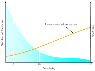
(a) popularity bias

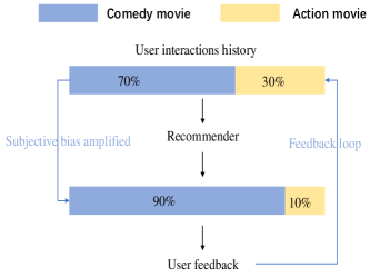
(b) amplified subjective bias

Figure 1: Popularity bias and amplified subjective bias.

Fig. 1(a) provides an example about the popularity bias in the real-world ML-20M dataset [30]. From the left y-axis, unpopular items (less than 50 interactions) account for the vast majority of the items, yet which are rarely recommended by the traditional recommendation models (e.g., the variational auto encoder(VAE) based model[14] represented by the orange line at the right y-axis). Influenced by the popularity bias, the Matthew effect[35] and the cold-start problem[40] are becoming increasingly commonplace in the recommender system. On the other hand, the amplified subjective bias[32] over-recommends the history preferences of users, misinterpreting the users’ current needs. As shown in Fig.1(b), given a user’s interaction history with 70% comedies and 30% action movies, the positive feedback loop[6] in the traditional recommenders exaggerates the user’s comedy preferences, increasing to 90% in the recommended films. Even worse, the amplified subjective bias also triggers some issues in the recommenders (e.g., filter bubbles[21] and echo chambers[9]), causing an ever-shrinking range of the recommended items.

Recently, a line of debias models have been proposed to alleviate these biases. For the popularity bias, the most common strategy is item reweighting, including highlighting unpopular items[16] or reducing the influence of popular items[15, 38]. While for the amplified subjective bias, existing models generally concentrate on adjusting the recommendation distribution from different aspects, including fairness[20, 31], diversity[5] and calibration[32]. Furthermore, some methods disentangle these biases by causal learning, e.g., the model-agnostic counterfactual reasoning framework (MACR)[39] or the deconfounded recommendation system (DecRS) [36], of which cause-effect strategy makes the debias process more reasonable and efficient.

Albeit much progress, the above debias methods still exhibit some defects. First is the single functionality. Existing methods are either designed for the popularity bias, or target to the amplified subjective bias. Such single debias methods neglect the bias-coupling probability, i.e., the items are recommended, perhaps collectively attributed to these two biases. In this way, adjusting any sole bias is accompanied by the excessive expressiveness of the other bias. Further, these bias-coupling recommended items cannot represent any pure bias, which easily causes the debias shift due to the coupled supervised signals. Besides, previous debias work doesn’t consider the data-sparsity problem in the recommender system, in which quantities of users have few historical interactions (as the sparsity metric shown in Table. LABEL:table1). In this light, insufficient interactions easily aggravate the difficulty of recognizing users’ preferences and recommendation biases.

To tackle the couple supervised issue brought by the single functionality, we propose a disentangled debias variational auto-encoder framework (DB-VAE) that decouples these two biases to help obtain a debias representation of user preferences. In particular, we first analyze the reason about the interaction between users and items, from which two direct causes of user click behavior are summarized: the item is popular and the item is matching the user’s preference. From this analysis, we design a casual graph about the user click behavior, helping disentangle the popularity bias and amplified subjective bias from the user’s interaction profile [24]. By defining the data split criterion of disentangled biases, two extreme types of items only affected by one bias can be extracted to further train the debias process, thereby mitigating the adverse effect of couple supervised signals. In addition, to address the data sparsity issue, we further design a counterfactual data generation strategy to produce massive counterfactual data, making up the lacking supervised signals due to the sparse interactions. In this generation process, a Pearl’s causal inference framework[26] is employed to help answer the questions about how will user perform if he or she is not affected by biases. Following the ’Abduction-Action-Prediction’ process, we answer the counterfactual questions and generate the corresponding counterfactual data, making up the lacking supervised signals.

We evaluate DB-VAE on three real-world RS datasets to verify its effectiveness. Extensive experimental results show that DB-VAE outperforms state-of-the-art baselines with average 5% improvements in terms of $NDCG$ and $Recall$. Furthermore, generating counterfactual data can further enhance DB-VAE, especially on sparser datasets. Overall, the contributions of this work can be summarized as the following three folds:

1. presenting a disentangled debias variational auto-encoder which simultaneously eliminates the popularity bias and the amplified subjective bias by two extreme types of items;

2. a counterfactual data generation method to make up the lacking supervised signals due to the data sparsity;

3. evaluations on three real-world datasets demonstrating the effectiveness and rationality of our proposed models.

2 Related work

In this section, we review existing recommendation debias work, mainly concentrating on the popularity bias and the amplified subjective bias.

2.1 Popularity Bias in Recommendation

In the recommender system, it is a common problem that users’ feedback is easily influenced by popular items. Recently, eliminating the popularity bias has received much attention in the recommendation research. Specifically, methods targeting to de-bias the popularity bias can be roughly divided into the following three types. The first line of the debias research aims at reweighting the popular items during training. For instance, Rosenbaum and Rubin [29] firstly propose an inverse propensity weighting (IPW) to adjust the importance of items according to their popularities. Inspired by this weighting strategy, Liang et al. [15] propose an improved method to impose lower weights on popular items. The second line of the debias research takes advantage of the ranking adjustment to calibrate the popularity bias. For example, Abdollahpouri et al. [1] introduce a regularization-based method to promote the rank of unpopular items. In addition, Abdollahpouri et al. [2] adopt a re-ranking strategy to adjust the output rank of the recommender system. The third line of the debias research employs the casual theory to alleviate the popularity bias, including the causal representation learning[18, 45] and the causal adjustment[43, 39].

Unlike the existing work, we argue that popularity bias should not be targeted singly because there is a complex coupled relationship between the popularity bias and the other biases. Hence, we introduce two extreme types of items to further train the debias process, thereby overcoming the blindness of debias brought by the couple biases.

2.2 Amplified subjective bias

During training, the positive feedback loop forces the recommender system to amplify the user’s historical preferences [6]. To correct such an amplified subjective bias, existing debias methods mainly explore from the following three aspects, i.e., fairness, diversity and causal recommendation. For the fairness in RS, Biega et al. [3] propose an amortized equity of attention, which ensures that similar individuals receive the similar treatments. And Morik et al. [20] argue all user groups are supposed to be treated fairly, thereby introducing a more granular way to keep the group fairness. Besides, Steck [32] re-rank the items to ensure the distribution of the recommended item groups to be matched with the users’ interaction history. For the diversity in RS, existing work pursues the dissimilarity of the recommended items [7, 34], where similarity can be measured by item category and embeddings[5, 12]. Furthermore, the causal recommendation targets to find the root reason for amplified bias. For example, Wang et al. [36] first scrutinize the cause-effect factors for bias amplification, and then contribute an approximation operator to eliminate the amplified subjective bias by the back-door adjustment.

However, the solely-modeling amplified subjective bias easily cause serious filter bubbles[21] and echo chambers[9]. Hence, we consider the amplified subjective bias combined with the other bias (mainly the popularity bias) during debias process. In this light, our proposed model eliminates the two types of bias simultaneously to disentangle the complex coupled relationship between these two biases.

3 Method

In this section, we first present the bias extraction in §3.1 to construct two extreme types of items only affected by a single bias. Then, we elaborate on the proposed DB-VAE model in §3.2, which helps accurately characterize the user’s debias latent representation and give debias predictions for user’s preferences. Finally, we introduce a counterfactual data generation method in §3.3 to enhance DB-VAE to tack the data sparsity issue.

3.1 Bias extraction

According to the causal theory [24], we design a causal graph on users’ interactions in Fig. 2. Clearly, there exist two direct causes (Node B and Node M) towards the users’ click behavior (Node C), i.e., the popularity of a specific item and the matching degree between this item and the target user. Although such two causes are independent in essence (Node B and Node M are not directly connected), their collider (Node C) makes them correlated in the expressive form of recommendation items. In this way, we expect to obtain the click-behavior data attributed to the sole cause. According to the colliding effect[25, 26], two extreme conditions can be extracted from user interactions, which reflect the popularity bias and the amplified subjective bias, respectively. In particular, if a user clicks on an item that hardly matches his/hers historical preferences, this click behavior is stemmed from the fact that this recommended item is very popular and the user is affected by conformity. And vice versa, an unpopular item gets clicked owing to its compatibility with the user’s personal preferences.

Figure 2: Causal graph on users interactions. Node C denotes the click behavior of user. Node B and Node M represent the popularity of the specific item and the matching degree between the item (Node I) and the user (Node U), respectively.

To measure the item popularity and the matching degree between users and items, the popularity score $S_{m}(u,i)$ and the matching score $S_{p}(u,i)$ between the target user $u$ and the recommended item $i$ are respectively introduced, as follows:

$$\left\{\begin{array}[]{ll}S_{p}(u,i)=\frac{num(i)}{\sum_{j\in{X}}num(j)},\\ S_{m}(u,i)=\frac{\textbf{d}_{i}\cdot\textbf{d}_{u}}{|\textbf{d}_{u}|},\end{array}\right.$$ (1)

where $X$ denotes the interaction profile with all items the target user $u$ clicked before and $num(i)$ is the click number of the item $i$ in the recommender system. And the popularity score $S_{p}(u,i)$ is defined as the ratio between the click number of the item $i$ and the click number summation of items the user $u$ clicked before. Besides, $\textbf{d}_{i}$ and $\textbf{d}_{u}$ denote the category representations of item $i$ and user $u$ by the one-hot format, respectively. In specific, given that there are five categories of movie tags in a movie dataset, including ’Comedy’,’Action’, ’Crime’, ’Adventure’ and ’Thriller’, the dimension of the category embeddings can be set to 5. In this way, when a movie has ’spider man’ has ’Comedy’ and ’Action’ tags, its category embeddings can be represented as $[1,1,0,0,0]$. While the user category embeddings are obtained by summarizing the category embeddings of all items the user has clicked on, i.e.,

$$\textbf{d}_{u}=\Sigma_{i\in X}\textbf{d}_{i},$$ (2)

Next, we elaborate on two extreme conditions from user interactions to obtain the sole-cause items. The first is the items that are clicked due to the conformity, which causes the popularity bias. So we select items that are very popular but rarely match the target user as $X_{p}$, i.e.,

$$X_{p}=\{i|rank(S_{p}(u,i))<k|X|,rank(S_{m}(u,i))>k|X|,i\in{X}\}$$ (3)

where $rank(S_{p}(u,i))$ and $rank(S_{m}(u,i))$ represents the ranking of the popularity score and the matching score of the item $i$ among all items clicked by the target user $u$, respectively; and $k\in[0,1]$ denotes the debias degree in which the smaller k indicates that less items are extracted from user’s interactions to construct $X_{p}$.

The second is the items that are clicked due to the user’s interests, which amplifies the subjective bias during the training process, and probably makes the recommender system fall into information cocoons[11]. Similarly, we select items that have a good match for the user’s interests, yet are rarely clicked by other users as $X_{m}$, i.e.,

$$X_{m}=\{i|rank(S_{p}(u,i))>k|X|,rank(S_{m}(u,i))<k|X|,i\in{X}\}$$ (4)

3.2 Debias variational auto-encoder

Variational auto-encoder(VAE) is a deep latent variable model[14, 28]. By the encoder-decoder structure, VAE can effectively learn latent representation from real-world data. Different from conventional auto-encoder(AE), VAE tries to ensure that the latent space is regular enough by introducing a distribution regularization during the training process. In this way, VAE can alleviate the over-fitting problem in conventional AE. In view of these merits, we select VAE as the backbone of DB-VAE in the hope that the standardized feature representation of users can be learned during the debias process. We present the framework of DB-VAE in Fig.3.

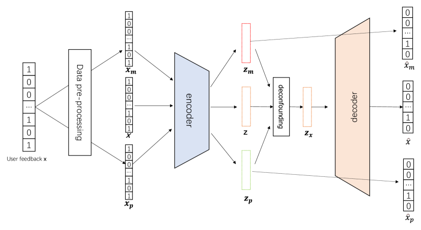
Figure 3: Framework of DB-VAE.

As shown in Fig.3, the total interacted items of the target user $X$, items $X_{p}$ attributed to the popularity bias and items $X_{m}$ attributed to the amplified subjective bias are taken as the input of VAE. And then, we employ the one-hot format embedding to encode $X$, $X_{m}$ and $X_{p}$, obtaining the corresponding embeddings $\bm{x}$, $\bm{x_{m}}$ and $\bm{x_{p}}$. These one-hot embeddings are further fed into the VAE encoder to generate their latent representations $\bm{z_{x}}$, $\bm{z_{m}}$ and $\bm{z_{p}}$, which can be formulated as follows:

$$\left\{\begin{array}[]{ll}\bm{z_{x}}\sim p_{\phi}(\bm{z_{x}}|\bm{x}),\\ \bm{z_{m}}\sim p_{\phi}(\bm{z_{m}}|\bm{x_{m}}),\\ \bm{z_{p}}\sim p_{\phi}(\bm{z_{p}}|\bm{x_{p}}),\end{array}\right.$$ (5)

where $\phi$ denotes the parameter set of the VAE encoder. Here, we select a 5-layer neural network as the VAEencoder. Furthermore, $\bm{z_{p}}$ and $\bm{z_{m}}$ can be treated as the user representations influence by the popularity bias and the amplified subjective bias, respectively. To reconstruct a user latent representation vector that is not affected by these two biases, we can obtain the unbiased user representation by subtracting $\bm{z_{p}}$ and $\bm{z_{m}}$ from $\bm{z_{x}}$, i.e.,

$$\bm{z}=\bm{z_{x}}-\bm{z_{m}}-\bm{z_{p}}$$ (6)

Different from the conventional auto-encoder, VAE assumes that the latent representation is subject to a prior standard normal distribution, from which a random sampling can be decoded to real-world data $\bm{x}$. However, the random sampling operation is not differentiable, which makes the model untrainable. In this light, we adopt the standard normal distribution $\mathcal{N}(\mu,\sigma^{2})$ as the posterior distribution generated by the encoder, and make the output of VAE approach this distribution by the KL divergence constraint during the model training. Formally, the output of the VAE encoder is subject to:

$$p_{\phi}(\bm{z_{x}}|\bm{x})=\mathcal{N}(\bm{{\mu}_{x}},\bm{{\sigma}_{x}}^{2}),$$ (7)

where

$$\left\{\begin{array}[]{ll}\bm{{\mu}_{x}}=g_{1}(f_{\phi}(\bm{x})),\\ log\bm{{\sigma}_{x}}^{2}=g_{2}(f_{\phi}(\bm{x})),\\ \end{array}\right.$$ (8)

in which $f_{\phi}()$ is a multilayer perceptron in the VAE encoder, $g_{1}()$ and $g_{2}()$ are two different fully connected layers of the VAE encoder. Analogously, the poster distributions $p_{\phi}(\bm{z_{m}}|\bm{x_{m}})$ and $p_{\phi}(\bm{z_{p}}|\bm{x_{p}})$ are generated in the same way. VAE takes the representation vectors $\bm{z_{x}}$, $\bm{z_{m}}$ and $\bm{z_{m}}$ as samples from the generated distribution $\mathcal{N}(\bm{{\mu}_{x}},\bm{{\sigma}_{x}}^{2})$, $\mathcal{N}(\bm{{\mu}_{m}},\bm{{\sigma}_{m}}^{2})$ and $\mathcal{N}(\bm{{\mu}_{p}},\bm{{\sigma}_{p}}^{2})$.

In order to ensure this operation is derivable, a re-parameterized way is adopted, which can be formulated as follows:

$$\left\{\begin{array}[]{ll}\bm{z_{x}}=\bm{\mu_{x}}+\bm{\epsilon}{\odot}\bm{\sigma_{x}},\\ \bm{z_{m}}=\bm{\mu_{m}}+\bm{\epsilon}{\odot}\bm{\sigma_{m}},\\ \bm{z_{p}}=\bm{\mu_{p}}+\bm{\epsilon}{\odot}\bm{\sigma_{p}},\end{array}\right.$$ (9)

where $\bm{\epsilon}$ is a sampled vector from multivariate standard normal distribution $\mathcal{N}(0,\bm{I})$ and $\odot$ is element-wise product operation. In this way, the sampling $\mathcal{N}(\bm{{\mu}_{x}},\bm{{\sigma}_{x}}^{2})$ is transformed to the sampling $\mathcal{N}(0,\bm{I})$. Hence, the operation ’sampling’ is not involved in the gradient descent, but in the result of sampling, making the whole model trainable. Under this sampling, the debiased user latent representation $\bm{z}$ in Eq. 6 can be transformed into:

$$\bm{z}=\bm{\mu_{x}}-\bm{\mu_{m}}-\bm{\mu_{p}}+\bm{\epsilon}{\odot}(\bm{\sigma_{x}}-\bm{\sigma_{m}}-\bm{\sigma_{p}})$$ (10)

With these laten representation, the final prediction score $\hat{\bm{x}}$ and the prediction scores of two biases ($\hat{\bm{x}}_{p}$ and $\hat{\bm{x}}_{m}$) can be decoded as follows:

$$\left\{\begin{array}[]{ll}\hat{\bm{x}}\sim q_{\theta}(\hat{\bm{x}}|\bm{z}),\\ \hat{\bm{x}}_{p}\sim q_{\theta}(\hat{\bm{x}}_{p}|\bm{z_{p}}),\\ \hat{\bm{x}}_{m}\sim q_{\theta}(\hat{\bm{x}}_{m}|\bm{z_{m}}),\end{array}\right.$$ (11)

where $\theta$ denotes the parameter set of the decoder.

Following the VAE training, the encoder parameter set $\phi$ and the decoder parameter set $\theta$ can be learned by maximizing the evidence lower bound (ELBO)[4]:

$$\mathcal{L}^{ELBO}(\hat{\bm{x}};\theta,\phi)=E_{p_{\phi}(\bm{z_{x}}|\bm{x},\bm{x_{p}},\bm{x_{m}})}[logq_{\theta}(\hat{\bm{x}}|\bm{z_{x}})-KL(p_{\phi}(\bm{z_{x}}|\bm{x},\bm{x_{p}},\bm{x_{m}})||p(\bm{z_{x}}))]$$ (12)

where the first half of this formula, $E_{p_{\phi}}[logq_{\theta}(\hat{\bm{x}}|\bm{z_{x}})]$ narrows the gap between $\bm{x}$ and $\hat{\bm{x}}$, and hence the cross entropy is employed to achieve this goal; the second part $KL(p_{\phi}(\bm{z_{x}}|\bm{x},\bm{x_{p}},\bm{x_{m}})||p(\bm{z_{x}}))$ represents the KL divergence between the posterior distribution $p_{\phi}(\bm{z_{x}}|\bm{x},\bm{x_{p}},\bm{x_{m}})$ and the prior distribution $p(\bm{z_{x}})$ with the assumption $p(\bm{z_{x}})\sim\mathcal{N}(0,\bm{I})$. By optimizing the negative KL divergence, DB-VAE can try to force that the debiased user feature representation $\bm{z_{x}}$ adheres to the standard normal distribution.

To overcome the issue of coupled supervised signals in the previous VAE training, we employ the bias-extracted data $X_{p}$ and $X_{m}$ to further train the VAE decoder, ensuring the accurate generation of $\bm{z_{m}}$ and $\bm{z_{p}}$:

$$\left\{\begin{array}[]{ll}\mathcal{L}^{s}(\hat{\bm{x_{p}}};\theta,\phi)=E_{p_{\phi(\bm{z_{p}}|\bm{x_{p}})}}[logq_{\theta}(\bm{\hat{x}_{p}}|\bm{z_{p})}],\\ \mathcal{L}^{s}(\hat{\bm{x_{m}}};\theta,\phi)=E_{p_{\phi(\bm{z_{m}}|\bm{x_{m}})}}[logq_{\theta}(\bm{\hat{x}_{m}}|\bm{z_{m})}],\\ \bm{x_{p}},\bm{x_{m}}=one-hot(X_{p}),one-hot(X_{m}),\end{array}\right.$$ (13)

where $one-hot(\cdot)$ is the one-hot embedding. All in all, the final loss can be jointly connected as:

$$\mathcal{L}=\mathcal{L}^{ELBO}(\hat{\bm{x}};\theta,\phi)+\omega_{m}\mathcal{L}^{s}({\bm{\hat{x}_{m}}};\theta,\phi)+\omega_{p}\mathcal{L}^{s}({\bm{\hat{x}_{p}};\theta,\phi)},$$ (14)

where $\omega_{m}$ and $\omega_{p}$ are weight parameters.

3.3 Counterfactual data generation

Intuitively, the direct way to mitigate the adverse effect of sparse data is to increase the data volume. To this end, we employ Pearl’s causal inference framework[26] to generate counterfactual data, in which this inference framework contains a three-layer causal hierarchy, including abduction, intervention and prediction.

Following this hierarchy, we first construct a basic model $\mathbf{F}$ abided by the causal graph proposed in Fig.2. Different from the causal graph, two exogenous variables $\alpha$ and $\beta$ are introduced to ensure the counterfactual prediction works. In specific, exogenous variables $\alpha$ and $\beta$ describe uncertainties that affect the matching degree in node $M$ and the popularity attribute in node $B$, respectively. For example, Santa movies are probably more popular around Christmas, revealing that the extra factor of date potentially influences the popularity. This indicates that there exist some uncertainties affecting the data generation process. Hence, the basic model $\mathbf{F}$ (as shown in Fig.4) is defined in a stochastic manner to consider the randomness and possible noisy data.

Figure 4: Casual graph with exogenous variables.

Formally, according to the inference process in Fig.4, the basic model $\mathbf{F}$ can be formulated as follows:

$$\mathbf{F}:\left\{\begin{aligned} &M\sim{p_{M}(M|U,I,\alpha)}\\ &B\sim{p_{B}(B|\beta)}\\ &C\sim{p_{C}(C|M,B)}\\ &\alpha,\beta\sim{\mathcal{N}(0,I)}\end{aligned}\right.,$$ (15)

where the distributions $p_{M}$, $p_{B}$ and $p_{C}$ can be detailed as:

$$\left\{\begin{array}[]{ll}M(u,i)=\frac{exp(\mathbf{E}_{u}^{T}\mathbf{E}_{i}+w_{i}^{M}\cdot S_{m}(u,i)\cdot\alpha_{i})}{\sum_{j}^{|\emph{I}|}exp(\mathbf{E}_{u}^{T}\mathbf{E}_{j}+w_{j}^{M}\cdot S_{m}(u,j)\cdot\alpha_{j})},\\ B(i)=\frac{exp(w_{i}^{B}\cdot S_{p}(u,i)\cdot\beta_{i})}{\sum_{j}^{|\emph{I}|}exp(w_{j}^{B}\cdot S_{p}(u,j)\cdot\beta_{j})},\\ C(u,i)=\frac{exp(M(u,i)+B(i))}{\sum_{j}^{|\emph{I}|}exp(M(u,j)+B(j))},\end{array}\right.$$ (16)

where $\mathbf{E}_{u}$ and $\mathbf{E}_{i}$ are the embeddings of user $u$ and item $i$ respectively; ${w}^{B}_{i}$ and ${w}^{M}_{i}$ are weighting parameters which can be learned during the training process, and $S_{m}(u,i)$ and $S_{p}(u,i)$ can be referred to Eq.(1).

With the observed dataset $\textit{O}=\cup_{i=1}^{|I|}\cup_{u=1}^{|U|}\{(x(u,i))\}$, the basic model $F$ can be learned by the cross entropy loss on the click prediction module $C(u,i)$, i.e.,

$$\mathcal{L}_{F}=\sum_{u}^{|U|}\sum_{i}^{|I|}[x(u,i)logC(u,i)]$$ (17)

where $x(u,i)$ is the ground truth indicating whether the user $u$ interacted with the item $i$. To ensure the randomness during th model training, $\mathbf{\alpha}$ and $\mathbf{\beta}$ are subject to the multivariate standard normal distribution $\mathcal{N}(0,I)$. Since the distribution of the observed data is highly influenced by $\mathbf{\alpha}$ and $\mathbf{\beta}$, the posterior distributions in different datasets are diverse. In this way, once we have learned $F$, we can follow the Pearl’s abduction-action-prediction framework[10] to generate counterfactual data, further strengthening the DB-VAE training.

In particular, the main objective of the abduction process is to estimate the posterior of $\mathbf{\alpha}$ and $\mathbf{\beta}$ from the observed dataset O. Taking $\mathbf{\alpha}$ as an example, its posterior can be computed by the following Bayesian rules:

$$p(\bm{\alpha}|\textit{O})\propto p(\bm{\alpha},\textit{O})=p(\bm{\alpha})p(\bm{\textit{O}|\alpha})$$ (18)

Unfortunately, the detail expressions of the prior distribution $p(\mathbf{\alpha})$ is unknown and too complex to be sampled. While the variational inference[4] can be a good solution to approximate $p(\mathbf{\alpha})$. In specific, $\bm{\alpha}$ is assumed to subject to a Gaussian distribution $q_{\phi}(\bm{\alpha})\sim\mathcal{N}(\bm{\mu},\bm{\sigma})$, where $\bm{\mu}$ and $\bm{\sigma}$ are learnable parameters. By minimizing the KL-divergence between $q_{\phi}(\bm{\alpha})$ and $p(\bm{\alpha}|\textit{O})$,the optimal $\bm{\mu}$ and $\bm{\sigma}$ can be obtained. This training process can be formulated as maximizing the evidence lower bound (ELBO)[4], i.e.,

$$\mathcal{L}^{ELBO}=E_{q_{\phi}(\bm{\alpha})}[\log p(\bm{\alpha},\textit{O})]-E_{q_{\phi}}[\log q_{\phi(\bm{\alpha})}(\bm{\alpha})]$$ (19)

Analogously, the distribution $p(\bm{\beta}|\textit{O})$ can also be learned by a similar way.

In the action step, we aim to figure out three counterfactual distributions $p_{C}(C|do(M),B)$, $p_{C}(C|M,do(B))$ and $p_{C}(C|do(M),do(B))$. Such three distributions answer three counterfactual questions, respectively, including 1) which items would a user interact with if he/she were not affected by the amplified subjective bias? 2) which items would a user like if he/she were not affected by the popularity bias? and 3) what would the user’s interaction behavior be if he is not affected by either bias? Besides, $S_{m}(u,i)$ is assumed to subject to the standard normal distribution $\mathcal{N}(0,1)$ and the $do(M)$ operation is realized by sampling $S_{m}(u,i)$ from $\mathcal{N}(0,1)$. Similarly, the operation $do(B)$ can be achieved by sampling $S_{p}(u,i)$ from $\mathcal{N}(0,1)$.

In the Prediction step, we employ the definition in Eq.(16) to generate three types of counterfactual distribution $p_{C}(C|do(M),B)$, $p_{C}(C|M,do(B))$ and $p_{C}(C|do(M),do(B))$. By selecting top-N items from these counterfactual distributions, we can construct counterfactual data $X^{counter}$, $X_{m}^{counter}$ and $X_{p}^{counter}$. The enhanced data can be obtained by combining counterfactual data with factual data, i.e.,

$$\left\{\begin{array}[]{ll}X^{en}=X\cup X^{counter},\\ X_{p}^{en}=X_{p}\cup X_{p}^{counter},\\ X_{m}^{en}=X_{m}\cup X_{m}^{counter},\end{array}\right.$$ (20)

By retraining DB-VAE with these enhanced data, the debias difficulty due to the data sparsity can be mitigated. In this work, we set $N=100$.

4 Experiments

In this section, we conduct experiments to evaluate the effectiveness of our proposed DB-VAE. To better guide our experimental analyses, we introduce four research questions (RQ)k, which are shown as follows:

• RQ1 Does our DB-VAE framework outperform other debiasing methods?

• RQ2 How do different debiasing components contribute to the performance? Can counterfactual data help improve the performance of DB-VAE?

• RQ3 How does DB-VAE perform in the item-user groups with different data sparsities?

• RQ4 How does the debiasing threshold value $k$ affect the performance of DB-VAE?

In addition, we first introduce the settings of experiment in §4.1, which includes the information about datasets, experimental setup, evaluation metrics and baseline models. Then, we elaborate on experimental results and present some analyses in §4.2, respectively answering the proposed research questions.

4.1 Experiment settings

4.1.1 Datasets

In this paper, we conduct experiments on three real-word recommendation datasets, including MovieLens [27, 44], AliShop-7C [19] and Amazon-book datasets[33]. In specific, MovieLens includes movie category information and user attribute information, which is a wildly-used dataset collected from MovieLens website. Given the different data sizes in MovieLens, we select ML-1M and ML-20M as our research datasets in this paper. AliShop-7C is collected from Taobao (Alibaba’s e-commerce platform). Amazon-book is one of Amazon product datasets[33], which records how users rate different books on Amazon. Among datasets used in our experiments, they all involve enough item features, e.g., the movie genre or the book category. More specifically, each dataset is filtered out items with less than 5 interactions and users with less than 2 interactions to ensure data quality. In addition, we list the information of all the datasets after pre-processing in Table LABEL:table1. From this table, we can find that Amazon-book is the sparsest dataset but has the largest number of categories, which may take great difficulty for model debiasing.

Table 1: Statistics of datasets, where the sparsity metric is calculated by dividing the number of actual interactions by the product of the user and item numbers. The held-out users is the number of validation/test users out of the total number of users in the first row

	ML-1M	Alishop-7c	ML-20M	Amazon-book
#total users	6034	10668	136677	482933
#item	3533	20591	20720	367963
#interactions	575272	767497	9990682	7145464
sparsity	2.70%	0.35%	0.35%	0.004%
#category	18	12	19	1600
#held-out users	800	1000	10000	40000

4.1.2 Experimental setup

To evaluate the model’s ability in constructing the user representation from the obvious interaction, we take all interactions of a specific user as a data instance. Specifically, we split all users into training/validation/test sets and the entire click histories from the training users are employed to train models. The #held-out users of Table LABEL:table1 indicates the number of validating/testing users. The 80% of the interactions of a validation user or a test user are used as the input of different models while the remaining 20% of the interactions are used to evaluate the model.

For the encoder of all models (i.e., $f_{\theta}()$ in Eq. 8), we choose a three-layer perceptions. And the decoder structure is the same as that of the encoder for the sake of symmetry. As the dimension setting in previous work[30], we set the dimensions of the latent representation and any hidden layer to 200 and 600, respectively. During the model training, we employ the Adam[13] optimizer with the batchsize of 500 users and apply a weight decay of 0.01. And we retain the models with the best $NDCG@100$ in the validation set and evaluate them on the test set.

4.1.3 Metrics

We adopt two classical ranking metrics in the recommender system as the evaluating metrics, including $Recall@K$ and $NDCG@K$ [23, 37], which are readily appropriate to the user data never appeared in the training set[36]. By comparing the top-k predictions with the ground-truth user $u$ in the test set $\bm{X}_{u}^{t}$, $Recall@K$ and $NDCG@K$ can be obtained.

In particular, we first sort the items in descending order of the predicted likelihood scores, and then select the top-K items with the highest score to form a recommendation list $\bm{R}_{u}$. Formally, $Recall@K(u)$ is defined as follows:

$$Recall@K(u)=\frac{\sum_{i=1}^{K}\mathbb{I}[R_{u}^{(i)}\in\bm{X}_{u}^{t}]}{min(K,|\bm{X}_{u}^{t}|)}$$ (21)

where $\mathbb{I}[\cdot]$ is an indicator function that returns 1 if the condition is satisfied. And the definition of $NDCG@K(u)$ is:

$$\left\{\begin{array}[]{ll}NDCG@K(u)=\Big{(}\sum_{i=1}^{|\bm{X}_{u}^{t}|}\frac{1}{log(n+1)}\Big{)}^{-1}DCG@k(u),\\ DCG@K(u)=\sum_{i=1}^{K}\frac{2^{\mathbb{I}[R_{u}^{(i)}\in\bm{X}_{u}^{t}]}}{log(n+1)},\end{array}\right.$$ (22)

where $NDCG@K(u)$ is defined as $DCG@K(u)$ divided by its theoretically possible value[30].

Generally, $Recall@K$ is large bigger than $NDCG@K$ under the same $K$, because $Recall@K$ treats equally all items in the top-K recommendation list, while $NDCG@K$ assigns larger weights to the top-ranked items. In this light, we select a larger $K$ for $NDCG@K$ than that for $Recall@K$ as previous work does[30, 17]. In specific, $Recall@20$ and $NDCG@100$ are adopted as evaluation metrics in our experiments.

4.1.4 Baselines

To verify the effectiveness of DB-VAE, we select several recent competitive recommendation models as the baselines, which can be further divided into two model groups. In particular, the first group is some well-designed VAE models [30, 17] without the debiasing operation. While the second group is model-agnostic debaising models [36, 39] which aim at eliminating either the popularity bias or the amplified subjective bias. More specifically,

• Mult-VAE[17] extends the variational autoencoder for learning implicit feedback in the top-k RS. By assuming that the user representation complies with the multivariate normal distribution, Mult-VAE introduces a different regularization parameter for the learning objective, achieving considerable performances.

• RecVAE[30] improves Mult-VAE by several optimization methods, including a novel composite prior distribution for the latent representation, a better approach to the weight setting in the evidence lower bound and a method of alternately updating parameters.

• MACR[39] is a model-agnostic framework that aims at eliminating the popularity bias in RS. MACR analyzes the cause-effect and introduces a multi-task learning method to answer the counterfactual question about what the ranking score would be if the model only uses item property. To fairly compare the model performance, we keep the backbone model of MACR the same as DB-VAE.

• DecRS[36] contributes an approximation operator by a backdoor adjustment, which concentrates on eliminating the obstacles in causal reasoning theory, thereby eliminating the amplified subjective bias. Similar to MACR, we keep the backbone model of DecRS same as DB-VAE.

4.2 Experimental results and analysis

This subsection respectively answers the proposed research questions by conducting the recommendation experiments about all discussed models on the selected datasets.

4.2.1 Overall performance.

For RQ1, we summarize the overall performance of our proposed DB-VAE as well as the selected baselines in terms of $Recall@20$ and $NDCG@100$ in Table.LABEL:table2. Generally, for any evaluation metric on any dataset, DB-VAE consistently shows a state-of-art performance. The detailed observations are presented as follows:

Table 2: Performance of DB-VAE as well as the selected baselines in terms of $Recall@20$ and $NDCG@100$. The bold font indicates the best performer in the belonged column.

Model	ML-1M		ML-20M		Alishop-7c		Amazon-book
	R@20	N@100	R@20	N@100	R@20	N@100	R@20	N@100
Mult-VAE	0.343	0.405	0.395	0.411	0.150	0.238	0.141	0.151
RecVAE	0.378	0.431	0.414	0.426	0.187	0.293	0.157	0.163
MACR(VAE)	0.391	0.441	0.432	0.437	0.195	0.298	0.159	0.164
DecRS(VAE)	0.395	0.449	0.442	0.439	0.206	0.305	0.162	0.165
DB-VAE(ours)	0.419	0.463	0.453	0.461	0.217	0.322	0.170	0.177

• In all cases, our disentangle debias framework boosts the performance of VAE models most obviously. Especially on Alishop-7c dataset, DB-VAE improves over 5% compared to the best baseline model in terms of both metrics. Even the smallest one on ML-20M dataset, DB-VAE can still achieve 2.4% improvements in terms of $Recall@20$. Such promising advancements over the vanilla VAE models or VAE-based debias models all demonstrate the effectiveness of DB-VAE.

• Clearly, VAE-based debias models (i.e., MACR, DecRS and DB-VAE) outperform vanilla VAE models (i.e., Mult-VAE, RecVAE), indicating that eliminating biases in the recommender system can be a good solution to improve the recommendation performance.

• Generally, all discussed models have worse performance on the datasets with a smaller sparsity, except on ML-1M. This finding reflects that sparser data can be easier to make wrong predictions. On the other hand, the exception ML-1M has more dense data than that of ML-20M, yet models don’t realize better performance on ML-1M. Such a contrast phenomenon may be attributed to the fact that the data volume is a more influential factor in the recommendation performance than the data sparsity. In other words, from the same data source, the data volume in ML-20M is 20 times of that in ML-1M, substantially making up the missing supervised signals brought by the data sparsity. This analysis can also be applicable to the comparison between Alishop-7c and ML-20M. In specific, despite the same data sparsity, the data volume of ML-20M is greater than that of Alishop-7c, and hence all discussed models have better performance on ML-20M than on Alishop-7c.

4.2.2 Ablation Study

Our proposed DB-VAE introduces a disentangled debias method that eliminates two different bias simultaneously. For answering RQ2, we first design two variants DB-VAE models by eliminating a specific type of bias. For example, DB-VAE(P) denotes the removal of the popularity bias in DB-VAE, where the only input of VAE is $X$ and $X_{p}$, and hence the user presentation in Eq.(6) is transformed into $\bm{z}=\bm{z_{x}}-\bm{z_{p}}$. Similarly, DB-VAE(M) represents DB-VAE without the amplified subjective debias component. To verify the effectiveness of counterfactual data, we further introduce a DB-VAE variant combined with the counterfactual data generation module, denoted as DB-VAE(CD). Besides, we add the best vanilla VAE model (RecVAE) into the performance comparison as the lower bound of these DB-VAE variants. With these discussed models, we summarize their performance on four different datasets in terms of $Recall@20$ and $NDCG@100$ in Table.LABEL:table3.

Table 3: Performance of DB-VAE variants, including replacing/removing a specific component and adding a counterfactual data enhencement.The bold font indicates the best performer in the belonged column. R@20 and N@100 are short for $Recall@20$ and $NDCG@100$, respectively.

Model	ML-1M		ML-20M		Alishop-7c		amazonbook
	R@20	N@100	R@20	N@100	R@20	N@100	R@20	N@100
RecVAE	0.378	0.431	0.414	0.426	0.187	0.293	0.161	0.167
DB-VAE(P)	0.383	0.445	0.417	0.429	0.189	0.297	0.151	0.163
DB-VAE(M)	0.352	0.423	0.421	0.433	0.185	0.295	0.157	0.165
DB-VAE	0.419	0.463	0.453	0.461	0.217	0.322	0.170	0.177
DB-VAE(CD)	0.407	0.438	0.459	0.471	0.219	0.326	0.181	0.195

Generally speaking, disentangled debias methods show superiority over the single debias one, i.e., original DB-VAE outperforms DB-VAE(P) and DB-VAE(M) on all datasets in terms of both metrics, reflecting that the disentangled debias methods are more appropriate and effective. In some extreme cases, the single debias variants are even worse than the model without debias components (i.e., RecVAE). For example, DB-VAE(M) is defeated by RecVAE on ML-1M dataset in terms of both metrics and on Alishop-7c dataset in terms of $Recall@20$. Such underperformance can be explained by the bias-coupling assumption in the introduction section, i.e., eliminating a single bias can instead cause the over-expressiveness of the other bias, further amplifying the adverse effect of the other bias. Furthermore, DB-VAE(P) outperforms DB-VAE(M) a lot on ML-1M with the greater data sparsity, while DB-VAE(M) takes the lead on ML-20M and amazonbook with the smaller data sparsity. This phenomena reflect that the data-intensive recommendation system is largely affected by the popularity bias; on the other hand, the amplified subjective bias plays a greater role in the data-sparse recommender.

Further, the generated counterfactual data can improve the performance of DB-VAE on all datasets except ML-1M, especially on amazonbook where DB-VAE(CD) achieve 6% and 10% improvements over original DB-VAE in terms of $Recall@20$ and $NDCG@100$, respectively. Such performance advancement indicate that counterfactual data is very appropriate to the data-sparse scenario, yet having a perverse effect on the data-intensive scenario. Such phenomena can be attributed to the fact that counterfactual data can help supplement the lacking supervised signals when data is sparse; however, for data with sufficient interactions, the addition of counterfactual data probably change the distribution of the original data, poisoning the model performance.

4.2.3 Performance on different sparsity groups

To further evaluate the models’ performance under different sparsity degrees (i.e., RQ3), we sorted the test users in ascending order according to the degree of sparsity(i.e., the number of interacted items), and then divided them equally into eight groups. In addition, we only test debias models in this subsection, including MACR, DecRS, DB-VAE and DB-VAE(CD). Their group performance are summarized in Fig.6.

(a) ML-1M

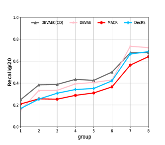
(b) ML-20M

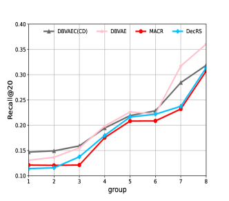
(c) Alishop-7c

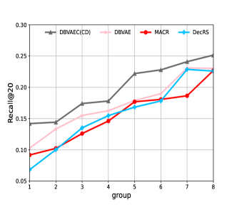
(d) amazonbook

Figure 5: Model performance on different sparsity groups in terms of Recall@20.

Clearly, with the increase of the sparsity value, all discussed models present an overall upward trend, indicating the data sparsity is an inherent problem that affects the recommendation performance and the smaller sparsity cause the worse model performance. In addition, DB-VAE(CD) always achieves a greater lead in the first group on all datasets, especially on amazonbook dataset, DB-VAE(CD) outperforms the original DB-VAE by nearly 40%. This phenomenon further verifies that counterfactual data can indeed help to improve the effectiveness of DB-VAE in the data-sparse scenario. On the other hand, DB-VAE becomes the best performer on ML-20M and Alishop-7c in the last two groups, demonstrating that our proposed method is most effective when there are sufficient data to support the model training.

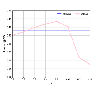
(a) ML-1M

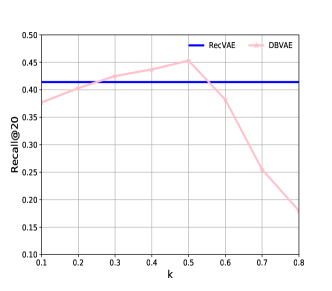
(b) ML-20M

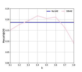
(c) Alishop-7c

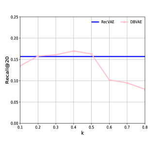
(d) amazonbook

Figure 6: Model performance on different sparsity groups in terms of Recall@20.

4.2.4 How $k$ affects the performance of DB-VAE?

The debias degree value $k$ in Eq.(3) and Eq.(4) controls the number of the items extracted from the user’s profile. The smaller the $k$ is, the fewer items we extract to debias. In this section, to answer RQ4, we evaluate how $k$ affects the performance of our proposed DB-VAE model. For simplicity, we present the change of model performance only in terms of $Recall@20$ since the performance in terms of $NDCG@100$ has similar trends. In addition, we also introduce the non-debias model RecVAE as the comparison benchmark to intuitively present the debias effect. Hence, we summarize the performance of DB-VAE and RecVAE affected by different debias degrees $K$ in terms of $Recall@20$ in Fig.LABEL:group_performance2.

Generally, DB-VAE presents a consistent change pattern, i.e., increasing first and then reducing. In addition, DB-VAE shows the best performance on two movielens datasets when $k$ is $0.5$, while peaks at $k=0.4$ on Alishop-7c and amazonbook, indicating that different datasets have respective preferences of bias degrees. Besides, when $k$ is small, e.g., $k=0.1$ and $k=0.2$, DB-VAE exhibits a little behind RecVAE in the model performance. As $k$ becomes bigger until the peak, the performance of DB-VAE constantly gets improved, exceeding RecVAE in some $k$ values. However, when $k$ is greater than $0.6$, DB-VAE presents a steep performance degeneration, creating a huge gap against RecVAE. These findings demonstrate that on one hand, slight debias cannot improve the model performance; on the other hand, excessive debias causes more damage to the model performance. Therefore, locating the appropriate debias degree becomes an important issue in future recommendation system research.

5 Conclusion

In this work, we explain the two most common biases in the recommender system, popularity bias and amplified subjective bias. To alleviate these biases, we propose a disentangled debias variational auto-encoder framework, which overcomes the shortcomings of other debias methods that are single and have no de-biased supervisory signals. In the process of debias, we make use of the relevant theory of causal inference, which helps us find the user interaction that may be biased. Extensive experiments validate that our proposed DB-VAE outperforms other debias methods. Also, we design a data enhancement method to help model training when data is sparse.

In future work, we will try to find the relationship between other types of biases and construct a unified and effective debias framework.

References

- Abdollahpouri et al. [2017] Himan Abdollahpouri, Robin Burke, and Bamshad Mobasher. Controlling popularity bias in learning-to-rank recommendation. In Proceedings of the eleventh ACM conference on recommender systems, pages 42–46, 2017.
- Abdollahpouri et al. [2019] Himan Abdollahpouri, Robin Burke, and Bamshad Mobasher. Managing popularity bias in recommender systems with personalized re-ranking. In The thirty-second international flairs conference, 2019.
- Biega et al. [2018] Asia J Biega, Krishna P Gummadi, and Gerhard Weikum. Equity of attention: Amortizing individual fairness in rankings. In The 41st international acm sigir conference on research & development in information retrieval, pages 405–414, 2018.
- Blei et al. [2017] David M Blei, Alp Kucukelbir, and Jon D McAuliffe. Variational inference: A review for statisticians. Journal of the American statistical Association, 112(518):859–877, 2017.
- Chandar and Carterette [2013] Praveen Chandar and Ben Carterette. Preference based evaluation measures for novelty and diversity. In Proceedings of the 36th international ACM SIGIR conference on Research and development in information retrieval, pages 413–422, 2013.
- Chaney et al. [2018] Allison JB Chaney, Brandon M Stewart, and Barbara E Engelhardt. How algorithmic confounding in recommendation systems increases homogeneity and decreases utility. In Proceedings of the 12th ACM Conference on Recommender Systems, pages 224–232, 2018.
- Cheng et al. [2017] Peizhe Cheng, Shuaiqiang Wang, Jun Ma, Jiankai Sun, and Hui Xiong. Learning to recommend accurate and diverse items. In Proceedings of the 26th international conference on World Wide Web, pages 183–192, 2017.
- Du et al. [2021] Yingpeng Du, Hongzhi Liu, and Zhonghai Wu. Modeling multi-factor and multi-faceted preferences over sequential networks for next item recommendation. In Joint European Conference on Machine Learning and Knowledge Discovery in Databases, pages 516–531. Springer, 2021.
- Ge et al. [2020] Yingqiang Ge, Shuya Zhao, Honglu Zhou, Changhua Pei, Fei Sun, Wenwu Ou, and Yongfeng Zhang. Understanding echo chambers in e-commerce recommender systems. In Proceedings of the 43rd international ACM SIGIR conference on research and development in information retrieval, pages 2261–2270, 2020.
- Glymour et al. [2016] Madelyn Glymour, Judea Pearl, and Nicholas P Jewell. Causal inference in statistics: A primer. John Wiley & Sons, 2016.
- Hou et al. [2021] Lei Hou, Xue Pan, Kecheng Liu, Zimo Yang, Jianguo Liu, and Tao Zhou. Information cocoons in online navigation. arXiv preprint arXiv:2109.06589, 2021.
- Jiang et al. [2020] Hao Jiang, Wenjie Wang, Yinwei Wei, Zan Gao, Yinglong Wang, and Liqiang Nie. What aspect do you like: Multi-scale time-aware user interest modeling for micro-video recommendation. In Proceedings of the 28th ACM International Conference on Multimedia, pages 3487–3495, 2020.
- Kingma and Ba [2014] Diederik P Kingma and Jimmy Ba. Adam: A method for stochastic optimization. arXiv preprint arXiv:1412.6980, 2014.
- Kingma and Welling [2014] Diederik P. Kingma and Max Welling. Auto-encoding variational bayes. In Yoshua Bengio and Yann LeCun, editors, 2nd International Conference on Learning Representations, ICLR 2014, Banff, AB, Canada, April 14-16, 2014, Conference Track Proceedings, 2014.
- Liang et al. [2016a] Dawen Liang, Laurent Charlin, and David M Blei. Causal inference for recommendation. In Causation: Foundation to Application, Workshop at UAI. AUAI, 2016a.
- Liang et al. [2016b] Dawen Liang, Laurent Charlin, James McInerney, and David M Blei. Modeling user exposure in recommendation. In Proceedings of the 25th international conference on World Wide Web, pages 951–961, 2016b.
- Liang et al. [2018] Dawen Liang, Rahul G Krishnan, Matthew D Hoffman, and Tony Jebara. Variational autoencoders for collaborative filtering. In Proceedings of the 2018 world wide web conference, pages 689–698, 2018.
- Liu et al. [2020] Dugang Liu, Pengxiang Cheng, Zhenhua Dong, Xiuqiang He, Weike Pan, and Zhong Ming. A general knowledge distillation framework for counterfactual recommendation via uniform data. In Proceedings of the 43rd International ACM SIGIR Conference on Research and Development in Information Retrieval, pages 831–840, 2020.
- Ma et al. [2019] Jianxin Ma, Chang Zhou, Peng Cui, Hongxia Yang, and Wenwu Zhu. Learning disentangled representations for recommendation. Advances in neural information processing systems, 32, 2019.
- Morik et al. [2020] Marco Morik, Ashudeep Singh, Jessica Hong, and Thorsten Joachims. Controlling fairness and bias in dynamic learning-to-rank. In Proceedings of the 43rd International ACM SIGIR Conference on Research and Development in Information Retrieval, pages 429–438, 2020.
- Nguyen et al. [2014] Tien T Nguyen, Pik-Mai Hui, F Maxwell Harper, Loren Terveen, and Joseph A Konstan. Exploring the filter bubble: the effect of using recommender systems on content diversity. In Proceedings of the 23rd international conference on World wide web, pages 677–686, 2014.
- Nie et al. [2019] Liqiang Nie, Meng Liu, and Xuemeng Song. Multimodal learning toward micro-video understanding. Synthesis Lectures on Image, Video, and Multimedia Processing, 9(4):1–186, 2019.
- Nie et al. [2020] Liqiang Nie, Yongqi Li, Fuli Feng, Xuemeng Song, Meng Wang, and Yinglong Wang. Large-scale question tagging via joint question-topic embedding learning. ACM Transactions on Information Systems (TOIS), 38(2):1–23, 2020.
- Pearl [2010] Judea Pearl. Causal inference. Causality: objectives and assessment, pages 39–58, 2010.
- Pearl and Mackenzie [2018] Judea Pearl and Dana Mackenzie. The book of why: the new science of cause and effect. Basic books, 2018.
- Peters et al. [2017] Jonas Peters, Dominik Janzing, and Bernhard Schölkopf. Elements of causal inference: foundations and learning algorithms. The MIT Press, 2017.
- Rendle et al. [2019] Steffen Rendle, Li Zhang, and Yehuda Koren. On the difficulty of evaluating baselines: A study on recommender systems. arXiv preprint arXiv:1905.01395, 2019.
- Rezende et al. [2014] Danilo Jimenez Rezende, Shakir Mohamed, and Daan Wierstra. Stochastic backpropagation and approximate inference in deep generative models. In Proceedings of the 31th International Conference on Machine Learning, ICML 2014, Beijing, China, 21-26 June 2014, volume 32 of JMLR Workshop and Conference Proceedings, pages 1278–1286. JMLR.org, 2014.
- Rosenbaum and Rubin [1983] Paul R Rosenbaum and Donald B Rubin. The central role of the propensity score in observational studies for causal effects. Biometrika, 70(1):41–55, 1983.
- Shenbin et al. [2020] Ilya Shenbin, Anton Alekseev, Elena Tutubalina, Valentin Malykh, and Sergey I Nikolenko. Recvae: A new variational autoencoder for top-n recommendations with implicit feedback. In Proceedings of the 13th International Conference on Web Search and Data Mining, pages 528–536, 2020.
- Singh and Joachims [2018] Ashudeep Singh and Thorsten Joachims. Fairness of exposure in rankings. In Proceedings of the 24th ACM SIGKDD International Conference on Knowledge Discovery & Data Mining, pages 2219–2228, 2018.
- Steck [2018] Harald Steck. Calibrated recommendations. In Proceedings of the 12th ACM conference on recommender systems, pages 154–162, 2018.
- Stratigi et al. [2019] Maria Stratigi, Xiaozhou Li, Kostas Stefanidis, and Zheying Zhang. Ratings vs. reviews in recommender systems: A case study on the amazon movies dataset. In European conference on advances in databases and information systems, pages 68–76. Springer, 2019.
- Sun et al. [2020] Jianing Sun, Wei Guo, Dengcheng Zhang, Yingxue Zhang, Florence Regol, Yaochen Hu, Huifeng Guo, Ruiming Tang, Han Yuan, Xiuqiang He, et al. A framework for recommending accurate and diverse items using bayesian graph convolutional neural networks. In Proceedings of the 26th ACM SIGKDD International Conference on Knowledge Discovery & Data Mining, pages 2030–2039, 2020.
- Wang et al. [2018a] Hao Wang, Zonghu Wang, and Weishi Zhang. Quantitative analysis of matthew effect and sparsity problem of recommender systems. In 2018 IEEE 3rd International Conference on Cloud Computing and Big Data Analysis (ICCCBDA), pages 78–82. IEEE, 2018a.
- Wang et al. [2021] Wenjie Wang, Fuli Feng, Xiangnan He, Xiang Wang, and Tat-Seng Chua. Deconfounded recommendation for alleviating bias amplification. In Proceedings of the 27th ACM SIGKDD Conference on Knowledge Discovery & Data Mining, pages 1717–1725, 2021.
- Wang et al. [2020] Xiang Wang, Hongye Jin, An Zhang, Xiangnan He, Tong Xu, and Tat-Seng Chua. Disentangled graph collaborative filtering. In Proceedings of the 43rd international ACM SIGIR conference on research and development in information retrieval, pages 1001–1010, 2020.
- Wang et al. [2018b] Yixin Wang, Dawen Liang, Laurent Charlin, and David M Blei. The deconfounded recommender: A causal inference approach to recommendation. arXiv preprint arXiv:1808.06581, 2018b.
- Wei et al. [2021a] Tianxin Wei, Fuli Feng, Jiawei Chen, Ziwei Wu, Jinfeng Yi, and Xiangnan He. Model-agnostic counterfactual reasoning for eliminating popularity bias in recommender system. In Proceedings of the 27th ACM SIGKDD Conference on Knowledge Discovery & Data Mining, pages 1791–1800, 2021a.
- Wei et al. [2021b] Yinwei Wei, Xiang Wang, Qi Li, Liqiang Nie, Yan Li, Xuanping Li, and Tat-Seng Chua. Contrastive learning for cold-start recommendation. In Proceedings of the 29th ACM International Conference on Multimedia, pages 5382–5390, 2021b.
- Wu et al. [2021] Chuhan Wu, Fangzhao Wu, Xiting Wang, Yongfeng Huang, and Xing Xie. Fairness-aware news recommendation with decomposed adversarial learning. In AAAI Conference on Artificial Intelligence, pages 4462–4469. AAAI Press, 2021.
- Zhang et al. [2022] Xiaokun Zhang, Bo Xu, Liang Yang, Chenliang Li, Fenglong Ma, Haifeng Liu, and Hongfei Lin. Price does matter! modeling price and interest preferences in session-based recommendation. arXiv preprint arXiv:2205.04181, 2022.
- Zhang et al. [2021] Yang Zhang, Fuli Feng, Xiangnan He, Tianxin Wei, Chonggang Song, Guohui Ling, and Yongdong Zhang. Causal intervention for leveraging popularity bias in recommendation. In Proceedings of the 44th International ACM SIGIR Conference on Research and Development in Information Retrieval, pages 11–20, 2021.
- Zheng et al. [2016] Yin Zheng, Bangsheng Tang, Wenkui Ding, and Hanning Zhou. A neural autoregressive approach to collaborative filtering. In International Conference on Machine Learning, pages 764–773. PMLR, 2016.
- Zheng et al. [2021] Yu Zheng, Chen Gao, Xiang Li, Xiangnan He, Yong Li, and Depeng Jin. Disentangling user interest and conformity for recommendation with causal embedding. In Proceedings of the Web Conference 2021, pages 2980–2991, 2021.
- Zhu et al. [2021] Ziwei Zhu, Yun He, Xing Zhao, and James Caverlee. Popularity bias in dynamic recommendation. In Proceedings of the 27th ACM SIGKDD Conference on Knowledge Discovery & Data Mining, pages 2439–2449, 2021.