Observational signatures of electron-driven chromospheric evaporation in a white-light flare

Abstract

We investigate observational signatures of explosive chromospheric evaporation during a white-light flare (WLF) that occurred on 2022 August 27. Using the moment analysis, bisector techniques, and the Gaussian fitting method, red-shifted velocities of less than 20 km s^-1 are detected in low-temperature spectral lines of H$\alpha$, C I  and Si IV  at the conjugated flare kernels, which could be regarded as downflows caused by chromospheric condensation. Blue-shifted velocities of $\sim$30$-$40 km s^-1 are found in the high-temperature line of Fe XXI , which can be interpreted as upflows driven by chromospheric evaporation. A nonthermal hard X-ray (HXR) source is co-spatial with one of the flare kernels, and the Doppler velocities are temporally correlated with the HXR fluxes. The nonthermal energy flux is estimated to be at least (1.3$\pm$0.2)$\times$10¹⁰ erg s^-1 cm^-2. The radiation enhancement at Fe I  6569.2 Å and 6173 Å suggests that the flare is a WLF. Moreover, the while-light emission at Fe I  6569.2 Å is temporally and spatially correlated with the blue shift of Fe XXI  line, suggesting that both the white-light enhancement and the chromospheric evaporation are triggered and driven by nonthermal electrons. All our observations support the scenario of an electron-driven explosive chromospheric evaporation in the WLF.

1 Introduction

Solar flares are detected as dramatic and impulsive electromagnetic emissions over a wide wavelength range on the Sun. In flares, energy which has been stored in nonpotential coronal magnetic field is released suddenly and converted to thermal energy of hot plasmas, kinetic energy of nonthermal particles, and bulk mass motions (Shibata & Magara, 2011; Benz, 2017; Jiang et al., 2021). The energy release is presumably caused by magnetic reconnection, as described by the two-dimensional (2-D) standard model (Priest & Forbes, 2002; Lin et al., 2005) or the CSHKP flare model (Carmichael, 1964; Sturrock, 1966; Hirayama, 1974; Kopp & Pneuman, 1976). In the vicinity of the reconnection region, the local plasma escapes in the form of bi-directional outflow jets, largely due to the strong curvature of reconnected magnetic field lines (e.g., Mann & Warmuth, 2011; Li, 2019; Warmuth & Mann, 2020; Li et al., 2021; Yan et al., 2022). They are usually turbulent and may contain plasmoids. The outflowing plasma is heated, and electrons are accelerated to nonthermal energies by a yet undetermined mechanism. Both heat conduction and accelerated electrons can provide a high energy flux into the dense chromosphere, which reacts with explosive heating and expansion. This results in hot plasma flowing up and quickly filling the newly formed flare loops, a process which is known as “chromospheric evaporation” (Fisher et al., 1985; Brosius & Daw, 2015; Dudík et al., 2016; Yang et al., 2021). Conversely, plasma can also slowly move downward due to momentum conservation, which is termed as “chromospheric condensation” (Kamio et al., 2005; Libbrecht et al., 2019; Graham et al., 2020; Yu et al., 2020).

Chromospheric evaporation exists in two variants: explosive and gentle. The two forms are sensitive to the incident energy flux, i.e., a threshold of 10¹⁰ erg s^-1 cm^-2 (e.g., Fisher et al., 1985; Kleint et al., 2016; Sadykov et al., 2019). It should be pointed out that the incident energy threshold will also depend on the location of energy deposition and the duration of heating (Reep et al., 2015; Polito et al., 2018), as well as the spectral parameters of the electrons (low-energy cutoff and slope). Explosive evaporation may also be driven by nonthermal electrons accelerated by a stochastic process at a low energy flux, i.e., $<$10¹⁰ erg s^-1 cm^-2 (Rubio da Costa et al., 2015). In the case of explosive chromospheric evaporation, chromospheric plasmas are rapidly heated, resulting in a much higher pressure in the chromosphere. Then, some plasmas expand upward into the low-density corona at fast velocities of several hundreds km s^-1, while some other plasmas precipitate downward with a slow velocity of a few tens km s^-1 into the high-density chromosphere due to momentum conservation (e.g., Veronig et al., 2010; Brosius & Inglis, 2017; Tian & Chen, 2018; Sellers et al., 2022). That is, the upflows driven by chromospheric evaporation and the downflows caused by chromospheric condensation can be simultaneously observed in an explosive evaporation event. In contrast, only the upflows can be seen for gentle evaporation. It is difficult to observe the downflows in gentle evaporation, which could be attributed to a much higher plasma density in the lower chromosphere (Doschek et al., 2013). Line profile spectroscopy is a good tool for diagnosing the chromospheric evaporation and condensation, which are often identified as the upflows of high-temperature plasmas in the corona and the downflows of low-temperature plasmas in the chromosphere, respectively (e.g., Teriaca et al., 2012; Doschek et al., 2013; Tian et al., 2014, 2021; Polito et al., 2017; De Pontieu et al., 2021). In spectroscopic observations (e.g., Ding et al., 1996; Milligan & Dennis, 2009; Li et al., 2015; Lee et al., 2017; Brosius & Inglis, 2018; Chen et al., 2022), the upflow is often identified as the blue-shifted Doppler velocity of hot lines at coronal heights, i.e., Fe XVIII , Fe XXI , etc., and the downflow is often regarded as the red shift of cool lines in the chromosphere or transition region, such as H$\alpha$, C I , Si IV , etc. Therefore, the gentle evaporation is characterized by blue shifts in all spectral lines (Milligan et al., 2006a; Li et al., 2019; Sadykov et al., 2019), while the explosive type is characterized by blue shifts in high-temperature lines and red shifts in low-temperature lines (Milligan et al., 2006b; Zhang et al., 2016; Brosius & Inglis, 2017).

Chromospheric evaporation can also be seen in soft X-ray (SXR) and Extreme Ultra-Violet (EUV) images (Liu et al., 2006; Ning & Cao, 2010; Ning, 2011), or observed in the radio dynamic spectrum (Aschwanden & Benz, 1995; Ning et al., 2009). The rapid mass motions originate from double footpoints along the flare loop and subsequently merge together at the loop-apex region. The moving speed could be equal to the upflow speed of hot evaporated materials. This phenomenon is regarded as the imaging evidence of chromospheric evaporation (e.g., Zhang et al., 2019; Li et al., 2022). The higher frequency suddenly suppresses and drifts to the lower frequency is regarded as the radio signature of chromospheric evaporation (Aschwanden & Benz, 1995). The chromospheric evaporation is frequently detected in the solar flare (Chen & Ding, 2010; Young et al., 2015; Polito et al., 2017; Libbrecht et al., 2019), and it can be observed during the precursor phase (Brosius & Holman, 2010; Li et al., 2018), the impulsive phase (Graham & Cauzzi, 2015; Li et al., 2017a; Sadykov et al., 2019) or the gradual phase (Czaykowska et al., 1999; Brannon, 2016). The similar evaporation phenomenon could also be found in the solar flare-like transient (Brosius & Holman, 2007) or the coronal bright point (Zhang & Ji, 2013; Li, 2022), because all these solar eruptive events are basically characterized by hot plasmas generated by the magnetic reconnection. Chromospheric evaporation can be driven by the nonthermal electrons (Tian et al., 2015; Warren et al., 2016; Lee et al., 2017), the thermal conduction (Battaglia et al., 2015; Ashfield & Longcope, 2021), or the dissipation of Alfvén waves (Reep & Russell, 2016; Van Damme et al., 2020). The electron-driven model emphasizes that nonthermal energies play a key role during the chromospheric evaporation, while the thermal conduction driven model states that thermal energies can directly cause the chromospheric evaporation.

A white-light flare (WLF) is a type of solar flare that shows a sudden enhancement in the white-light continuum, which was first reported by Carrington (1859) and Hodgson (1859). White-light emission is often thought to be formed in the lower atmosphere on the Sun, but the generation mechanism of white-light emission is still unclear (Aboudarham & Henoux, 1989; Fang et al., 2013). Several heating mechanisms have been discussed in the literature, for instance nonthermal electron bombardment (Hudson, 1972), thermal irradiation (Henoux & Nakagawa, 1977), and chromospheric condensation (Gan & Mauas, 1994). Recently, magnetic reconnection in the lower solar atmosphere has been proposed to power a WLF (Song et al., 2020). In this paper, we explore observational signatures of explosive chromospheric evaporation during a WLF, which are consistent with the electron-driven model. Section 2 presents instruments and observations. Section 3 describes data analyses and results. Section 4 offers a brief discussion, and Section 5 summarizes our conclusion.

2 Instruments and Observations

The solar flare studied in this work occurred on 2022 August 27 in the active region of NOAA 13088 (S26W66). It was simultaneously measured by the Chinese H$\alpha$ Solar Explorer (CHASE; Li et al., 2022), the Interface Region Imaging Spectrograph (IRIS; De Pontieu et al., 2014), the Atmospheric Imaging Assembly (AIA; Lemen et al., 2012) and the Helioseismic and Magnetic Imager (HMI; Schou et al., 2012) aboard the Solar Dynamics Observatory (SDO), the Spectrometer/Telescope for Imaging X-rays (STIX; Krucker et al., 2020) on Solar Orbiter (Müller et al., 2020), the Gravitational wave high-energy Electromagnetic Counterpart All-sky Monitor (GECAM; Xiao et al., 2022), the Geostationary Operational Environmental Satellite (GOES), and the STEREO/WAVES (SWAVES), as listed in table 1.

CHASE is designed to acquire the spectroscopic observations at wavebands of H$\alpha$ and Fe I . The scientific payload is the H$\alpha$ Imaging Spectrograph (HIS), which has two observational modes: raster scanning mode (RSM) and continuum imaging mode (CIM). Here, the RSM data products are used for analysis, and they provide full-Sun spectral images at wavelength ranges of 6559.7 Å$-$6565.9 Å (H$\alpha$) and 6567.8 Å$-$6570.6 Å (Fe I ). In normal observation, the spectral dispersion is 24 mÅ pixel^-1, and the pixel scale is 0.52″ (Qiu et al., 2022). For the in-orbit binning data applied in this study, the spectral and spatial resolutions are twice lower than nominal. The time cadence is about 71 s. IRIS is a space-based multi-channel UV imaging spectrograph mainly focused on the solar chromosphere and transition region (De Pontieu et al., 2014). On 2022 August 27, IRIS observed the active region in a large “sit-and-stare” mode with a time cadence of $\sim$9.4 s. The pixel scale along the slit is $\sim$0.166″. Here, we use the spectral lines at IRIS windows of “O I  1356 Å” and “Si IV  1403 Å”, and the Slit-Jaw Imager (SJI) at 1400 Å. The far ultraviolet (FUV) spectra at “O I ” and “Si IV ” had a spectral dispersion of 25.96/25.44 mÅ pixel^-1. SJI 1400 Å images had a field-of-view (FOV) of 119″$\times$119″ with a time cadence of 28.2 s. SDO/AIA is designed to take full-disk solar images in multiple wavelengths nearly simultaneously (Lemen et al., 2012). SDO/HMI is designed to investigate the solar magnetic field and oscillatory features on the Sun (Schou et al., 2012). Here, the AIA images at seven EUV channels of 94 Å, 131 Å, 171 Å, 193 Å, 211 Å, 304 Å, and 335 Å are used, which have a time cadence of 12 s. We also use the continuum filtergram and the line-of-sight (LOS) magnetogram of SDO/HMI, which have a time cadence of 45 s. The AIA and HMI maps have been calibrated by using the standard programs of aia_prep.pro and hmi_prep.pro, respectively, and thus they all have a spatial scale of 0.6″ pixel^-1.

STIX provides X-ray imaging spectroscopy of solar flares over an energy range of 4$-$150 keV and thus characterizes both the hot and super-hot flare plasmas as well as the accelerated nonthermal electrons (Krucker et al., 2020). In this study, we use two different STIX data products. The spectrogram data, which is generated on-board by summing over all pixels in all detectors, is used to generate HXR countrates in wider energy bins, such as 4$-$10 keV, 10$-$15 keV, and 15$-$25 keV. The advantage of this data type is that we can use the full temporal resolution of STIX, which was 0.5 s in this event. In contrast, the pixelated science data is obtained by downlinking the counts for all pixels in all detectors individually. We use this data set to generate disk-integrated spectrograms and to reconstruct HXR images. For this event, the time resolution of the pixelated data was set at 20 s in order to ensure statistically significant numbers of counts in all pixels. We wanted to state that all STIX times have been modified in order to be consistent with the observations from 1 AU, as Solar Orbiter was at 0.79 AU in this event.

GECAM is designed to monitor high-energy astrophysical features, i.e., searching for gravitational waves, detecting $\gamma$-ray bursts. It consists of 25 Gamma Ray Detectors (GRD) and 8 Charged Particle Detectors (CPD). GECAM/GRD can also provide the solar irradiance measurement in hard X-rays and $\gamma$-rays (Xiao et al., 2022). In this study, the solar HXR flux at the high gain channel such as 20$-$60 keV is used for analysis, which has an uniform time cadence of 0.2 s.

3 Analyses and Results

3.1 Overview of the solar flare

Figure 1 shows an overview of X-ray light curves integrated over the entire Sun during 13:00$-$13:30 UT on 2022 August 27. Panel (a) presents SXR fluxes recorded by GOES in 1$-$8 Å (red) and 0.5$-$4 Å channel (blue). It shows a C9.6 class flare that begins at about 13:06 UT, reaches its maximum at around 13:13 UT, and stops at 13:17 UT, as indicated by the red vertical lines. Both GOES fluxes reveal two main peaks, implying two episodes of energy releases. The background image is the radio dynamic spectrum measured by SWAVES at lower frequencies between 0.023 MHz and 16.025 MHz. The radio spectrum does not show any signature of solar radio bursts, suggesting that there are not nonthermal electrons escaping from the flare region. The temporal resolution of SWAVES is one minute, but it still can resolve the presence of type III radio bursts at lower frequencies. Moreover, we do not see any signature of type III radio bursts in solar dynamic spectra of e-Callisto with high temporal resolution (i.e., $\leq$1 s). No coronal mass ejection (CME) was detected after the C9.6 flare. All those facts suggest that it is a confined flare. Figure 1 (b) plots the X-ray light curves measured by STIX at 4$-$10 keV (black), 10$-$15 keV (orange), and 15$-$25 keV (green), and GECAM 20$-$60 keV (cyan), respectively. It can be seen that all the light curves show two main pulses, similarly to what has observed by GOES. Moreover, the second pulse is much stronger than the first one, and we fucus on the second HXR pulse, which spans from the impulsive phase to the gradual phase of the C9.6 flare.

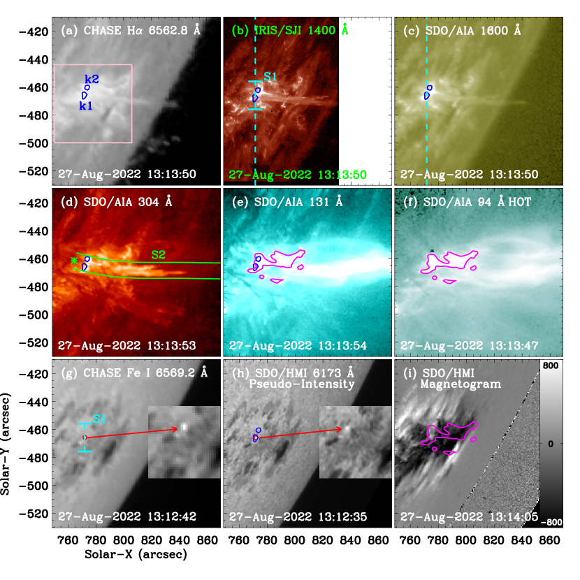
Figure 2: Snapshots in multiple wavebands with a same FOV of 120″$\times$120″ measured by CHASE/HIS (a, g), IRIS/SJI (c), SDO/AIA (c$-$f), and SDO/HMI (h, i). Blue and magenta contours outline bright kernels/features in H$\alpha$ and AIA 94 Å hot channels. The pink box and two short cyan lines mark the flare region, and the dashed cyan line (S1) represents the slit of IRIS. The green (S2) curves outline the solar jet, which are used to perform the time-distance maps in Figure 7. The red arrow indicates an enhancement of the white light radiation. Two zoomed images show Fe I  6569.2 Å and HMI pseudo-intensity maps with a small FOV of about 30″$\times$30″.

In Figure 2, we present multi-wavelength maps with a same FOV of 120″$\times$120″. Panel (a) shows the H$\alpha$ map at 6562.8 Å during the flare observed by CHASE, which reveals two bright flare kernels (k1 and k2), as outlined by the blue contours. They could be regarded as the conjugated footpoints of a hot flare loop. Panels (b) plots the FUV image captured by IRIS/SJI in 1400 Å, while panels (c) and (d) draw UV/EUV images observed by SDO/AIA at wavelengths of 1600 Å and 304 Å. They all exhibit two bright and compact kernels, which match well with double H$\alpha$ kernels, as indicated by the blue contours. Therefore, these maps at wavelengths of H$\alpha$ 6562.8 Å, SJI 1400 Å, and AIA 1600 Å are used to co-align between different instruments. The dashed cyan line marks the slit of IRIS, which goes through one flare kernel (i.e., k1). A solar jet originated from the loop-apex appear simultaneously in those four images, and it is most vivid in AIA 304 Å, as outlined by two green lines.

Figures 2(e) and 2(f) show EUV maps at high-temperature channels of AIA 131 Å and 94 Å. A short flare loop that connects to the double H$\alpha$ kernels (blue contours) can be seen in AIA 131 Å. It is well known that the two AIA channels in 131 Å and 94 Å are sensitive to hot plasmas, but a strong contribution from cool plasmas is also found in these two channels (e.g., O’Dwyer et al., 2010). Therefore, we utilize the approach following the Equation 1 to extract the hot plasma from AIA 94 Å (cf. Del Zanna, 2013; Gupta et al., 2018).

$$I_{\rm hot}\approx I({\rm 94~{}{\AA}})-\frac{I({\rm 171~{}{\AA}})}{450}-\frac{I({\rm 211~{}{\AA}})}{120},$$ (1)

Where, I(94 Å), I(171 Å), and I(211 Å) represent intensities measured by SDO/AIA at the corresponding wavelengths. Panel (f) shows the EUV map at AIA 94 Å hot channel, and the short flare loop can be seen at the high-temperature channel, as indicated by the magenta contour. Moreover, it links to the conjugated footpoints that root in positive and negative magnetic fields, respectively, as shown in panel (i).

Figures 2(g) and 2(h) present white-light images measured by CHASE and SDO/HMI during the C9.6 flare, respectively. The CHASE map at Fe I 6569.2 Å reveals one bright feature, as outlined by the red contour. This bright feature could be considered as the enhancement of white-light radiation, and it can be also seen in the pseudo-intensity map, as shown in the two zoomed images. We should state that the pseudo-intensity map is made from SDO/HMI continuum filtergrams at two adjacent times, since it is easier to observe the white-light enhancement even when it is rather weak (cf. Song et al., 2018; Li et al., 2023). The formation height of Fe I  line at 6569.2 Å is estimated to be in the mid-photosphere around 250 km for the quiet Sun (cf. Hong et al., 2022). Therefore, the C9.6 flare is indeed a white-light flare. Moreover, the white-light enhancement locates in one H$\alpha$ kernel that scanned by the IRIS slit, as indicated by the dashed cyan line. Here, we also generate the time-distance images along the IRIS slit (short dashed cyan line) that derived from the CHASE maps at Fe I  6569.2 Å and H$\alpha$ 6562.8 Å.

3.2 CHASE spectra

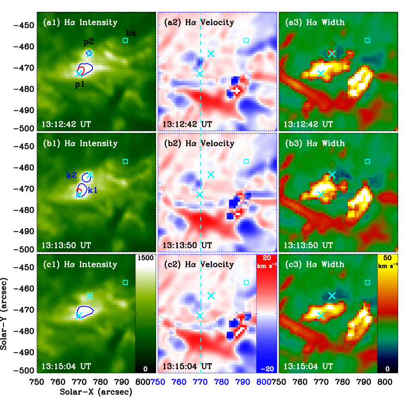
Figure 3: Moment analysis results (line intensity, Doppler velocity, and line width) from CHASE H$\alpha$ spectra during the C9.6 flare. They all have a small FOV of 56″$\times$56″, as outlined by the pink box in Figure 2 (a). Blue and red contours represent the H$\alpha$ line intensity and Fe I  emission, respectively. Two cyan crosses (‘$\times$’) and one box mark the locations to show H$\alpha$ spectra at flare kernels and non-flare (background) region in Figure 4. The dashed cyan line represents the slit of IRIS.

Two flare kernels (k1 and k2) can be seen in the CHASE H$\alpha$ map at 6562.8 Å, and the IRIS slit covers one of them (i.e., k1), as shown in Figure 2. The H$\alpha$ spectrum, which is recorded by the CHASE full-Sun raster scanning, contains the spectral and spatial information of the Sun and can be used to investigate the double flare kernels. Based on the moment analysis technique (e.g., Brannon, 2016; Li et al., 2017b, 2020), the 2-D maps of line intensity, Doppler velocity and width at H$\alpha$ waveband can be obtained, which are determined from the zeroth, first, and second moments (cf. Yu et al., 2020). Figure 3 shows H$\alpha$ maps for the line intensity (left), Doppler velocity (middle), and line width (right) at three times during the C9.6 flare. They all have a FOV of about 56″$\times$56″, as outlined by the pink box in Figure 2 (a).

Similarly to what one sees in the H$\alpha$ map at 6562.8 Å, the line intensity maps basically reveal two flare kernels, as shown in Figure 3 (a1)$-$(c1). The k2 kernel appears and enhances from 13:12:42 UT to 13:13:50 UT, then it becomes very weak and gradually disappears at about 13:15:04 UT. At the same time, the k1 kernel can always be seen from 13:12:42 UT to 13:15:04 UT during the C9.6 flare, and it is much stronger than the k2 kernel. The white-light emission at CHASE Fe I  shows one bright source, which is co-spatial with the H$\alpha$ kernel k1, as indicated by the red contour in panel (a1). However, the white-light emission only lasts for a short time, and becomes weak at 13:13:50 UT and gradually disappears at 13:15:04 UT, as shown in panels (b1) and (c1). The Doppler velocities of these two kernels are dominated by red shifts, as shown in Figure 3 (a2)$-$(c2), and their Doppler velocities are small, i.e., $<$10 km s^-1. Their line widths are also enhanced at two flare kernels, and the line width at k1 kernel is significantly stronger than that at k2 kernel. The feature of Doppler velocities and line widths implies that the chromospheric condensation is simultaneously observed at two flare kernels. We also note that the red-shifted velocity tends to appear at the outer edge of flare kernels, which is similar to previous observations (Czaykowska et al., 1999; Li & Ding, 2004)

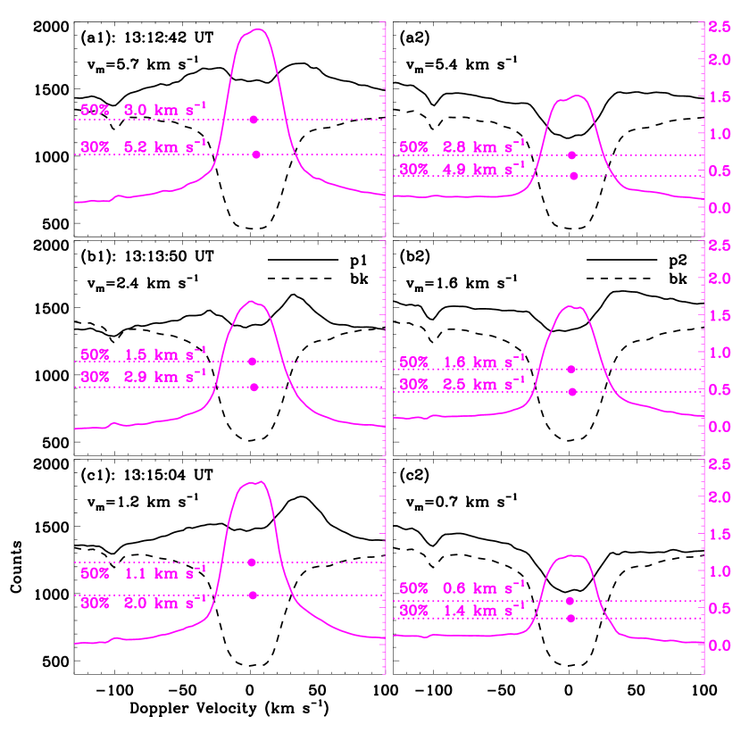
Figure 4: H$\alpha$ spectra observed by CHASE/HIS in flare kernels (solid black) and non-flare region (dashed black) at three time. The solid magenta curves indicate the H$\alpha$ contrast line profiles, as normalized by the background spectrum. The dotted magenta lines represent emission levels, and the bisector velocities are indicated by solid dots.

In order to look closely at the H$\alpha$ spectrum, Figure 4 presents the line profiles of H$\alpha$ at the locations of two kernels and the background (no-flare region), as marked by the crosses and box in Figure 3. The black solid and dashed lines represent H$\alpha$ line profiles at flare kernels and background, respectively. Similar to previous observations (e.g., Ding et al., 1994; Li & Ding, 2004), the H$\alpha$ line cores at flare kernels are central-reversed. The H$\alpha$ line profile at the background seems to be symmetrical. At the same time, those line profiles at flare kernels appear to be extremely asymmetrical, and the enhancement at the red-wing is stronger than that at the blue-wing, confirming the red-shifted velocities at flare kernels. To measure their Doppler shifts, we perform the moment analysis technique (e.g., Li et al., 2017b; Yu et al., 2020) to the H$\alpha$ contrast line profiles, which are derived from the Equation 2:

$$C(\lambda)=(I_{\rm k}(\lambda)-I_{\rm b}(\lambda))/I_{\rm b}(\lambda),$$ (2)

Where $C(\lambda)$ represents the contrast H$\alpha$ line profile as a function of the wavelength ($\lambda$), $I_{\rm k}(\lambda)$ and $I_{\rm b}(\lambda)$ are H$\alpha$ line profiles at the flare kernel and background, respectively. The magenta curves in Figure 4 are H$\alpha$ contrast line profiles at flare kernels, and they all demonstrate red shifts of less than 10 km s^-1. The smallest velocity is found at the k2 kernel at 13:15:04 UT (c2), and the line intensity and width are also very weak. This is consistent with the observation fact that the H$\alpha$ emission here is very weak.

As is known, the moment method only provides averaged parameters. In order to further confirm the Doppler velocities at two H$\alpha$ kernel positions, we also perform the bisector method to the emission components of H$\alpha$ contrast line profiles (cf. Ding et al., 1995; Hong et al., 2014; Ishikawa et al., 2020). In this method, the Doppler velocity is calculated from the shift of the line center relative to the rest wavelength, and the line-center shift is determined as the middle point’s wavelength of the H$\alpha$ contrast line profile ($C$) at a given emission level ($q$), such as $q*(C_{max}-C_{min})+C_{min}$. Here, $C_{max}$ and $C_{min}$ represent the maximal and minimal values of the H$\alpha$ contrast emission. The dotted magenta lines in Figure 4 indicate 50% and 30% emission levels, and their bisector velocities are also marked by the magenta dots. Obviously, the bisector velocities are sensitive to emission levels, but they all reveal red shifts at slow velocities, i.e., $<$10 km s^-1, which are comparable to the moment velocities ($v_{m}$). Thus, we can conclude that the two H$\alpha$ kernels show red shifts, and they could be regarded as downflows caused by chromospheric condensation.

3.3 IRIS spectra

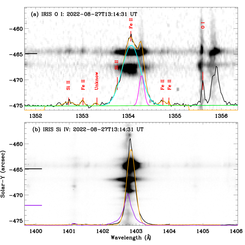
Figure 5: IRIS spectra at two FUV windows of ‘O I ’ (a) and ‘Si IV ’ (b) on 2022 August 27. The black profiles are line spectra at the flare kernel, as marked by the short black line on the left side of each panel, and the overplotted orange profiles represent their best-fitting results. The cyan and magenta lines are Fe XXI  and C I , and the green line is the fitting background. The red vertical ticks labeled some other emission lines used in this study. The purple curve (after multiplication by 10) is the line spectrum at non-flare location, as marked by the short purple line.

In order to study the flare kernel (i.e., k1) in details, we then analyse IRIS spectral lines, including Fe XXI , C I , and Si IV . The forbidden transition of Fe XXI  line is a potentially useful diagnostic for high-temperature ($\sim$11 MK) plasmas during the solar flare, while the chromospheric line of C I  can be used for the diagnostics of low-temperature ($\sim$0.01 MK) plasmas. However, these two and some other emission lines in the considered spectral window are blended (e.g., Tian et al., 2015; Young et al., 2015; Li et al., 2016; Polito et al., 2016; Tian, 2017). Thus, we utilize multi-Gaussian function superimposed on a linear background to fit the IRIS spectrum (cf. Li et al., 2015, 2017a, 2018). Figure 5 (a) presents the IRIS spectrum in the window of “O I ” during the C9.6 flare. It can be seen that a broad line is blended with some other emission lines, as indicated by the short vertical red lines. Here the emission line O I is applied for absolute wavelength calibration (Tian et al., 2015). The orange line represents the best-fitting results by using the multi-Gaussian function, which matches well with the observed line spectrum. The green line is the linear background, while the cyan and magenta lines indicate the line profiles of Fe XXI  and C I , respectively. In the IRIS window of “Si IV ”, the transition line of Si IV  is isolated, and it is much stronger than other emission lines during the solar flare, as shown in Figure 5 (b). Thus, we use a single-Gaussian function (orange) to fit the line spectrum (black). The reference wavelength of Si IV  is determined from the non-flare region, as indicated by the purple line. On the other hand, the reference wavelength of Fe XXI  cannot be determined from the non-flare region, because it is a hot flare line. So, the reference wavelength of Fe XXI  is selected as 1354.1 Å (cf. Young et al., 2015). Then the Doppler velocity of each emission line can be determined by subtracting the fitted line center from its reference wavelength.

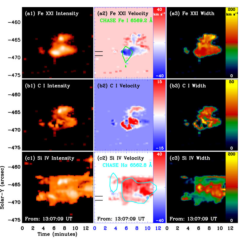
Figure 6: Time-distance images of line intensity, Doppler velocity and line width from IRIS spectra, e.g., Fe XXI , C I , and Si IV . Two short black lines outline the flare region used to integrate the time series in Figure 8. Green and cyan contours represent the CHASE observations at Fe I  and H$\alpha$. A logarithmic scale is used for the line intensity.

Figure 6 shows time-distance diagrams of line intensity, Doppler velocity and line width for Fe XXI , C I , and Si IV , respectively. The displayed images have the same length of about 20″ along the IRIS slit, as indicated by two short cyan line in Figure 2 (b). From the left panels, we notice that a very weak FUV emission appears in the flare kernel during the first HXR pulse, i.e., $\sim$13:09$-$13:11 UT. Then, a strong FUV emission is seen at these three emission lines, which corresponds to the second HXR pulse. During the second HXR pulse, the Doppler velocity of Fe XXI  line tends to show blue shifts of $\sim$30$-$40 km s^-1, while that of C I  and Si IV  lines appears to show red shifts of $\sim$10$-$20 km s^-1, as shown in the middle panels. Their line widths are all broad at flare kernels, as shown in the right panels. We note that the speeds of hot evaporating plasmas measured from Fe XXI line blueshifts are pretty weak, which is in disagreement with the expectation for explosive chromospheric evaporation. This is mainly because the solar flare studied in this work occurred close to the solar limb (e.g., S26W66), and thus the Doppler shifts are strongly affected by the projection effect. Moreover, the chromospheric evaporation corresponds the second HXR pulse, so the Fe XXI line blueshifts could be seriously influenced by the falling velocity of hot evaporating plasmas during the first HXR pulse. We also derived time-distance images along the IRIS slit (Figure 2g) from the CHASE data series at Fe I  6569.2 Å and H$\alpha$ 6562.8 Å, as shown by the overlaid green and cyan contours in panels (a2) and (c2). It can be seen that the Fe I  6569.2 Å emission source is co-spatial with the blue-shifted velocity of Fe XXI line at the flare kernel k1, while the H$\alpha$ 6562.8 Å emission source is spatially correlated with the red-shifted velocity of Si IV line at two flare kernels. The feature of Doppler velocities and line widths suggests an explosive chromospheric evaporation, namely the chromospheric evaporation and condensation are simultaneously detected during the C9.6 flare. The explosive chromospheric evaporation occurs nearly simultaneously with the white-light enhancement.

3.4 Solar jet

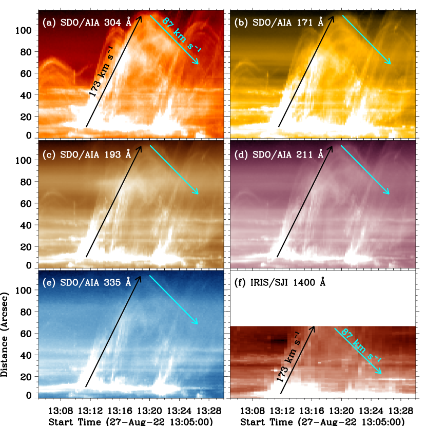
Figure 7: Time-distance images along the solar jet, which are performed from SDO and IRIS maps at wavelengths of AIA 304 Å (a), 171 Å (b), 193 Å (c), 211 Å (d), and 335 Å (e), and SJI 1400 Å (f). The black and cyan arrows indicate the rise and fall speeds of the solar jet.

A solar jet ejects from the flare loop-apex region, as shown in Figure 2. To investigate its evolution, we draw the time-distance images along the propagation direction of the jet, as outlined by two green curves in Figure 2 (d). Here, a constant width of $\sim$12″ is used, so that the bulk of the jet can be covered as much as possible during its whole lifetime. Figure 7 presents the time-distance images at wavelengths of AIA 304 Å, 171 Å, 193 Å, 211 Å, and 335 Å, and SJI 1400 Å. The solar jet firstly propagates outward following after the C9.6 flare, and the apparent speed is estimated to about 173 km s^-1. Then some material of the solar jet falls back with an apparent speed of about 87 km s^-1. The whole evolution of this jet could be seen in several AIA EUV channels, suggesting that the solar jet is characterized by multi-temperature plasma structures, which is similar to previous results (e.g., Lu et al., 2019; Shen, 2021). IRIS/SJI did not observe the whole solar jet, but similar speeds of propagating and falling are detected, as shown in panel (f). The dynamics of the jet suggest that there is no mass ejecting from the Sun during the C9.6 flare, which is consistent to the absence of the matching CME in the catalog. Therefore, the C9.6 flare is probable a confined flare.

4 Discussion

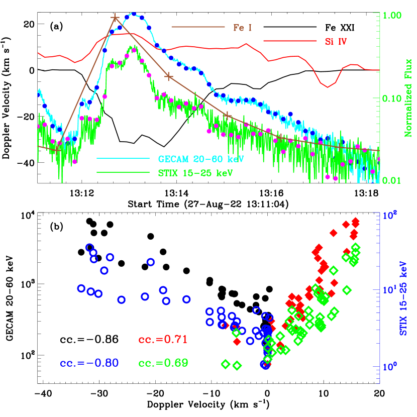
Figure 8: Time series of the Doppler velocity in Fe XXI  (black) and Si IV  (red), and normalized HXR fluxes at GECAM 20$-$60 keV (cyan) and STIX 15$-$25 keV (green), and the normalized white light flux at CHASE Fe I (brown). The blue and magenta dots mark these HXR points used to perform the correlation analysis. Panel (b): Scatter plots of Doppler velocities of Fe XXI  (circles) and Si IV  (diamonds) depend on the HXR fluxes observed by GECAM (fill) and STIX (hollow). Their Pearson correlation coefficients (cc.) are labeled.

In this section, we discuss the physical mechanism of the explosive chromospheric evaporation. Figure 8 plots the correlation between HXR emissions and Doppler velocities. Panel (a) presents the temporal evolution of Doppler velocities in Fe XXI  (black) and Si IV (red), the normalized white-light flux at CHASE Fe I  6569.2 Å (brown), and the normalized HXR fluxes at STIX 15$-$25 keV (green) and GECAM 20$-$60 keV (cyan) during 13:11:04$-$13:18:14 UT, respectively. The flare line of Fe XXI  exhibits blueshifts, while the transition region line of Si IV  reveals redshifts, and their maximum velocities are about 33 km s^-1 and 16 km s^-1, respectively. The white-light flux seems to be temporally correlated with the Doppler velocities of Fe XXI  and Si IV , and it is also consistent with HXR fluxes recorded by GECAM and STIX, implying that both white-light emission and chromospheric evaporation could be associated with nonthermal electrons. The Doppler velocities and white-light flux are averaged over the flare kernel (k1), as indicated by the two short black lines in Figure 6. These curves appear to show a good correlation with each other, but they have different time cadences (Table 1), making it impossible to correlate them directly. Thus, we interpolate HXR fluxes to the IRIS time cadence, as indicated by solid dots. It should be pointed out that we do not interpolate the white-light flux, due to its very low time resolution. We then show the dependence of Doppler velocities of Fe XXI  (circles) and Si IV  (diamonds) on HXR fluxes at GECAM 20$-$60 keV (fill) and STIX 15$-$25 keV (hollow), as shown in Figure 8 (b). High Pearson correlation coefficients are found between the Doppler velocities of Fe XXI  and HXR emissions at GECAM 20$-$60 keV (-0.86) and STIX 15$-$25 keV (-0.80), ‘$-$’ means that the Doppler velocities of Fe XXI  are blueshifts. The Pearson correlation coefficients between red-shifted velocities of Si IV  and HXR fluxes are 0.71 and 0.69, respectively. Such high correlation coefficients indicate that the explosive chromospheric evaporation is probably driven by nonthermal electrons accelerated by magnetic reconnection (e.g., Li et al., 2015, 2017a; Tian et al., 2015).

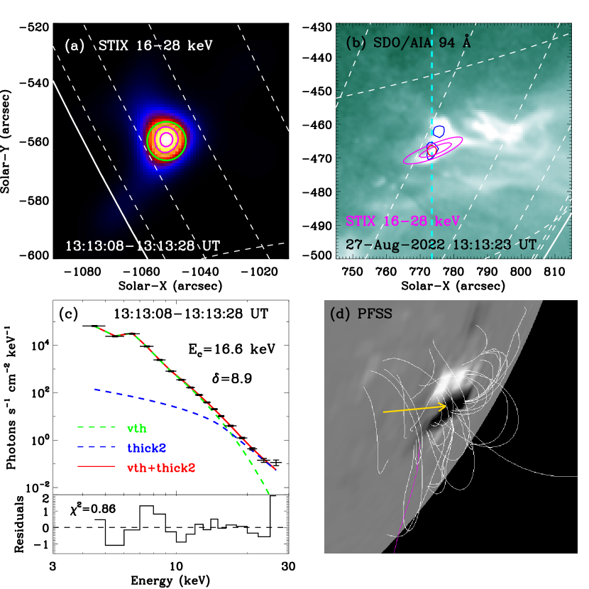
Figure 9: Panels (a) and (b): STIX 16$-$28 keV and AIA 94 Å maps during the solar flare. The magenta contours represent HXR emissions at levels of 70%, and 90%. The dashed white lines indicate latitude-longitude grids, and the solid white line marks the solar limb. The green circle is an visibility forward-fit for the HXR source area. The cyan dashed line outlines the IRIS slit, the blue and red contours denotes to H$\alpha$ and Fe I kernels. Panel (c): STIX X-ray spectrum between 4-28 keV with an integrated time of 20 s, the fitted thermal (green) and nonthermal (blue) components, as well as the sum of both components (red). The low-energy cutoff ($E_{c}$), spectral index ($\delta$), and the chi-squared residual ($\chi^{2}$) are labeled. Panel (d): The magnetic configuration from the SDO viewpoint with a PFSS model. The white and purple lines represent the closed and open magnetic field, respectively. The gold arrow indicates the short flare loop.

To determine the energy flux that is deposited in the chromosphere during the evaporation process, we need to constrain both the electron flux and the footpoint area. We start by reconstructing the nonthermal HXR source in the energy range of 16$-$28 keV with the STIX pixelated science data using the Expectation Maximization algorithm (Massa et al., 2019). The resulting source is shown in Figure 9 (a), with the contour levels set at 70% and 90% of the maximum intensity. It should be pointed out that Solar Orbiter was located 147 degrees from the Earth_Sun line, so in contrast to the near-Earth observations, the flare is seen here near the east limb. As was already evident from the observations in the other wavelength range, this flare is very compact, and we therefore cannot separate it into the expected double footpoint structures. As the STIX source is rather circular, we performed an additional image reconstruction using the Visibility Forward Fit method (Volpara et al., 2022) with a circular source, as indicated by the overplotted green circle. The advantage of this method is that it returns the fit parameters with error estimates, and so we derive a nonthermal source area ($A$) of (4.1$\pm$0.7)$\times$10¹⁷ cm². Since we most probably do not resolve the source, this has to be considered as an upper limit.

While normally the precise HXR source locations are provided by the STIX Aspect System (Warmuth et al., 2020), Solar Orbiter was too far from the Sun (e.g., 0.79 AU) to get a reliable pointing solution. We therefore reconstructed a thermal HXR image (6$-$10 keV) and co-aligned it with a co-temporal EUV image at 174 Å captured by the Full Sun Imager (FSI) of the Extreme Ultraviolet Imager (EUI; Rochus et al., 2020) on Solar Orbiter. Figure 9 (a) already shows the corrected source location. In order to compare the nonthermal STIX source to the other observations, we reproject the STIX image to the Earth view assuming the source is located on the solar surface, which is justified for a chromospheric footpoint source. This was performed using version 4.1.5 of the SunPy open source software package (SunPy Community et al., 2020). Figure 9 (b) shows the reprojected STIX source overplotted on a co-temporal AIA 94 Å image. The apparent elongation of the source is a projection artefact due to the fact that we do not resolve the east-west extension of the source. However, we can see that the centroid of the reprojected source appears to be coincident with the location of one H$\alpha$ kernel and the Fe I source, as indicated by the magenta, blue, and red contours, respectively. Thus, it could be regarded as one footpoint of a short flare loop seen in AIA 94 Å. Our observation is consistent with previous findings, i.e., white-light kernels are typically found to be co-spatial with HXR sources (Metcalf et al., 2003; Cheng et al., 2015; Yurchyshyn et al., 2017). Moreover, the IRIS slit (dashed cyan line) crosses the H$\alpha$ kernel and HXR source, confirming that the explosive evaporation is caused by nonthermal electrons, which is similar to previous observations (e.g., Zhang et al., 2016; Li et al., 2018).

In the next step, we constrain the energy input rate provided by the injected nonthermal electrons by fitting the STIX count spectra in the range of 4$-$28 keV with the combination of an isothermal component and a thick-target power-law. This is performed with the OSPEX spectral analysis package using the functions VTH and THICK2, with the addition of an albedo component. Figure 9 (c) shows a fitted spectrum for a representative time interval during the nonthermal HXR peak (13:13:08$-$13:13:28 UT). In the plot, we indicate the low-energy cutoff energy (E_c) and the spectral index ($\delta$) of the injected electron flux. The $\chi^{2}$ value and the residuals plotted in the lower part of the figure indicate a good fit result. Note that the nonthermal spectrum is very soft. The cutoff energy of 16.6 keV confirms that the STIX X-ray radiation at 16$-$28 keV is mainly from the nonthermal emission, thus the area ($A$) of nonthermal source could be about (4.1$\pm$0.7)$\times$10¹⁷ cm². Next, the nonthermal power ($P$) above the cutoff energy could be calculated by the code in SolarSoftWare, such as “calc_nontherm_electron_energy_flux.pro”, which is about 5.2$\times$10²⁷ erg s^-1. At last, the nonthermal energy flux ($P/A$) can be estimated to be about (1.3$\pm$0.2)$\times$10¹⁰ erg s^-1 cm^-2. This is just a bit larger than the critical threshold of deposited energy flux given by Fisher et al. (1985). However, we have to consider our result as a lower estimate only. We use the highest low-energy cutoff that is consistent with the data, therefore our electron flux is a lower estimate. Since the true low-energy cutoff is masked by the thermal emission, the total electron flux could be considerably higher. On the other hand, the HXR source is most probably not well resolved, so the footpoint area could well be smaller. Since both effects will result in a higher energy flux, we conclude that the STIX observations support the explosive chromospheric evaporation scenario.

In this flare, the HXR spectrum at higher energies is so steep (i.e.,$\delta$=8.9) that it may actually be consistent with a hotter secondary thermal component as opposed to injected electrons with a soft spectrum. To investigate this possibility, we also fitted the STIX spectrum that showed a high-energy tail with double-thermal components. For the time interval shown in Fig. 9 (c), this resulted in a cooler component with a temperature ($T$) of $(16.4\pm 0.5$) MK and an emission measure ($EM$) of ($2.8\pm 0.3)\times 10^{48}$ cm^-3, and a hotter component with $T=(31.9\pm 4.3)$ MK and $EM=(1.7\pm 1.7)\times 10^{46}$ cm^-3. It is evident that the hotter component is significantly less well constrained than the cool one. However, the strongest argument against the interpretation of the high-energy tail as a hotter thermal component is the cooling time, which should be as short $\approx$2 minutes in order to explain the quickly vanishing high-energy tail in the observed spectrum. To estimate the cooling time of the hotter component, we use the model of Cargill et al. (1995). This is based on conductive and radiative cooling timescales assuming an isotropic, isothermal, collisionless plasma. Apart from temperature, the model requires the electron density and the loop half-length as input. We get a density of $\sim$$9\times 10^{9}$ cm^-3 from the EM of the hotter component and the source volume, which we derive from the forward-fitted circular source assuming spherical geometry. Taking the footpoints of the loop structure seen in the AIA 94 Å image and assuming a semicircular loop, we obtain a loop half-length of about 7 Mm. For these parameters, the Cargill model predicts a time of $\sim$11 minutes for the plasma to cool from $\sim$32 MK down to $\sim$16 MK, which is significantly longer than the observed decay time of the high-energy tail of the spectrum. Even when we assume a very small filling factor of just 0.01 for the hotter component (which results in higher densities and thus more efficient cooling), the predicted cooling time is still $\sim$7 minutes. In summary, the observations are indeed more consistent with a nonthermal thick-target model.

In order to look closely at the magnetic field topology on the source surface that connects to the flare region, we perform a potential field source surface (PFSS) extrapolation to the synoptic SDO/HMI map, as shown in Figure 9 (d). We notice that the flare area is dominated by closed magnetic field lines (white lines), preventing electron beams generated from the C9.6 flare to escape into the interplanetary space. Therefore, we can not observe the radio III burst at lower frequencies, as shown in Figure 1 (a). So, the C9.6 flare is confined rather than eruptive. Moreover, some closed magnetic lines appear at the region of the short flare loop seen in AIA 94 Å, as indicated by the gold arrow. This further suggests the presence of flare loop that connects double H$\alpha$ kernels.

5 Summary

Based on multi-wavelength observations measured by CHASE, IRIS, SDO/AIA, SDO/HMI, STIX, GECAM, and SWAVES, we investigate explosive chromospheric evaporation during a C9.6 flare on 2022 August 27. The main conclusions are summarized as following:

1. The H$\alpha$ spectroscopic observations obtained with CHASE reveal two flare kernels, which are connected by a short flare loop seen in the high-temperature channel of AIA (131 Å and 94 Å). Two loop legs are rooted in positive and negative magnetic fields, respectively. Thus, they are recognized as conjugated footpoints. The double kernels (k1 and k2) show red-shifted velocities of less than 10 km s^-1 in H$\alpha$ Doppergrams. One kernel (k1) exhibits red shifts of 10$-$20 km s^-1 in the cool lines of C I  and Si IV  detected by IRIS. Those red shifts can be regarded as the downflows driven by chromospheric condensation (Li & Ding, 2004; Zhang et al., 2016; Libbrecht et al., 2019; Graham et al., 2020; Li et al., 2022).

2. One flare kernel (k1) shows blue shifts of 30$-$40 km s^-1 in the hot line of Fe XXI . The blueshift could be the indicator of the upflow caused by chromospheric evaporation (Brosius & Daw, 2015; Dudík et al., 2016). Interestingly, the blue-shifted velocity is co-spatial with the white-light emission captured by CHASE at Fe I  6569.2 Å, implying that the chromospheric evaporation and white-light emission have the same driver. We also notice that the velocity of upflows is rather small compared to previous findings (Veronig et al., 2010; Li et al., 2015; Young et al., 2015; Tian & Chen, 2018), which could be due to the fact that the WLF was located at the solar limb, or because that the chromospheric evaporation spans from impulsive phase to the gradual phase of the C9.6 flare.

3. The chromospheric condensation and evaporation are simultaneously observed during the C9.6 flare, implying an explosive chromospheric evaporation. A lower boundary for the nonthermal energy flux is estimated to be (1.3$\pm$0.2)$\times$10¹⁰ erg s^-1 cm^-2, confirming the explosive chromospheric evaporation (e.g., Fisher et al., 1985; Li et al., 2018; Sadykov et al., 2019). We also considered alternative fittings to the STIX spectrum with double-thermal components. However, the cooling time is too long for the hotter plasma that is required.

4. High correlations are found between Doppler velocities of Fe XXI  and Si IV  and the HXR emission at GECAM 20$-$60 keV and STIX 15$-$25 keV. Moreover, the nonthermal deposited energy source seen at STIX 16$-$28 keV is coincident with one flare kernel seen in H$\alpha$ and Fe I wavebands. All those observational facts indicate that the explosive chromospheric evaporation is driven by nonthermal electrons that accelerated by the magnetic reconnection (e.g., Tian et al., 2015; Warren et al., 2016; Zhang et al., 2016; Lee et al., 2017; Li et al., 2017a).

5. The CHASE map at Fe I  6569.2 Å shows a white-light enhancement at one flare kernel (k1), and the similar enhancement is also detected in the pseudo-intensity map derived from SDO/HMI continuum filtergrams (cf. Song et al., 2018). Thus, the C9.6 flare is indeed a white-light flare. The white-light flux at Fe I  6569.2 Å appears to be temporally correlated with the HXR flux, indicating that the white-light emission is induced by nonthermal electrons. PFSS extrapolation based on the synoptic SDO/HMI map suggests that the flare area is characterized by closed magnetic field lines. No flare-related lower-frequency radio III burst or CMEs are observed, and a jet originated from the loop-apex finally falls back, suggesting that the white-light flare is also a confined flare (e.g., Song et al., 2014; Kliem et al., 2021).

Table 1: Details of observational instruments used in this paper.

Instruments	Windows	Wavelengths	Spectral Dispersion	Cadence	Spatial resolution1
	H$\alpha$	6559.7$-$6565.9 Å	$\sim$48 mÅ	$\sim$71 s	2.08″
CHASE	Fe I	6567.8$-$6570.6 Å	$\sim$48 mÅ	$\sim$71 s	2.08″
	O I	1351.42$-$1356.61 Å	25.96 mÅ	$\sim$9.4 s	0.33″
IRIS/SP	Si IV	1398.66$-$1407.00 Å	25.44 mÅ	$\sim$9.4 s	0.33″
IRIS/SJI	FUV	1400 Å	–	$\sim$28.2 s	0.33″
	EUV	94$-$335 Å	–	12 s	1.2″
SDO/AIA	UV	1600 Å	–	24 s	1.2″
	Magnetogram	6173 Å	–	45 s	1.2″
SDO/HMI	Continuum	6173 Å	–	45 s	1.2″
	SXR	1$-$8 Å	–	1 s	–
GOES	SXR	0.5$-$4 Å	–	1 s	–
	LC	4$-$10 keV	–	0.5 s	–
	LC	10$-$15 keV	–	0.5 s	–
STIX	LC	15$-$25 keV	–	0.5 s	–
	Spectra	4$-$28 keV	$\sim$1 keV	20 s	–
	Pixel	16$-$28 keV	–	20 s	11.5″
GECAM	HXR	20$-$60 keV	–	0.2 s	–
SWAVES	Radio	0.023$-$16.025 MHz	–	60 s	–

• ¹The spatial resolution here is seen from Earth, i.e., 1 AU.

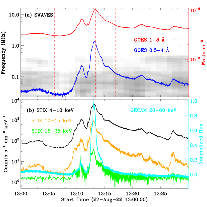
Figure 1: Full-disk light curves from 13:00 UT to 13:30 UT on 2022 August 27. Panel (a): GOES SXR fluxes at wavelengths of 1$-$8 Å (red) and 0.5$-$4 Å (blue). The context image is the radio spectrogram observed by SWAVES. Panel (b): STIX count fluxes in the energy bands of 4$-$10 keV (black), 10$-$15 keV (orange), and 15$-$25 keV (green), and the normalized GECAM flux at 20$-$60 keV (cyan).

References

- Aboudarham & Henoux (1989) Aboudarham, J. & Henoux, J. C. 1989, Sol. Phys., 121, 19. doi:10.1007/BF00161685
- Aschwanden & Benz (1995) Aschwanden, M. J. & Benz, A. O. 1995, ApJ, 438, 997. doi:10.1086/175141
- Ashfield & Longcope (2021) Ashfield, W. H. & Longcope, D. W. 2021, ApJ, 912, 25. doi:10.3847/1538-4357/abedb4
- Battaglia et al. (2015) Battaglia, M., Kleint, L., Krucker, S., et al. 2015, ApJ, 813, 113. doi:10.1088/0004-637X/813/2/113
- Benz (2017) Benz, A. O. 2017, Living Reviews in Solar Physics, 14, 2. doi:10.1007/s41116-016-0004-3
- Brannon (2016) Brannon, S. R. 2016, ApJ, 833, 101. doi:10.3847/1538-4357/833/1/101
- Brosius & Holman (2007) Brosius, J. W. & Holman, G. D. 2007, ApJ, 659, L73. doi:10.1086/516629
- Brosius & Holman (2010) Brosius, J. W. & Holman, G. D. 2010, ApJ, 720, 1472. doi:10.1088/0004-637X/720/2/1472
- Brosius & Daw (2015) Brosius, J. W. & Daw, A. N. 2015, ApJ, 810, 45. doi:10.1088/0004-637X/810/1/45
- Brosius & Inglis (2017) Brosius, J. W. & Inglis, A. R. 2017, ApJ, 848, 39. doi:10.3847/1538-4357/aa8a68
- Brosius & Inglis (2018) Brosius, J. W. & Inglis, A. R. 2018, ApJ, 867, 85. doi:10.3847/1538-4357/aae5f5
- Cargill et al. (1995) Cargill, P. J., Mariska, J. T., & Antiochos, S. K. 1995, ApJ, 439, 1034. doi:10.1086/175240
- Carmichael (1964) Carmichael, H. 1964, NASA Special Publication, 451
- Carrington (1859) Carrington, R. C. 1859, MNRAS, 20, 13. doi:10.1093/mnras/20.1.13
- Chen & Ding (2010) Chen, F. & Ding, M. D. 2010, ApJ, 724, 640. doi:10.1088/0004-637X/724/1/640
- Chen et al. (2022) Chen, H., Tian, H., Li, H., et al. 2022, ApJ, 933, 92. doi:10.3847/1538-4357/ac739b
- Cheng et al. (2015) Cheng, X., Hao, Q., Ding, M. D., et al. 2015, ApJ, 809, 46. doi:10.1088/0004-637X/809/1/46
- Czaykowska et al. (1999) Czaykowska, A., De Pontieu, B., Alexander, D., et al. 1999, ApJ, 521, L75. doi:10.1086/312176
- Del Zanna (2013) Del Zanna, G. 2013, A&A, 558, A73. doi:10.1051/0004-6361/201321653
- De Pontieu et al. (2014) De Pontieu, B., Title, A. M., Lemen, J. R., et al. 2014, Sol. Phys., 289, 2733. doi:10.1007/s11207-014-0485-y
- De Pontieu et al. (2021) De Pontieu, B., Polito, V., Hansteen, V., et al. 2021, Sol. Phys., 296, 84. doi:10.1007/s11207-021-01826-0
- Doschek et al. (2013) Doschek, G. A., Warren, H. P., & Young, P. R. 2013, ApJ, 767, 55. doi:10.1088/0004-637X/767/1/55
- Ding et al. (1994) Ding, M. D., Fang, C., & Okamoto, T. 1994, Sol. Phys., 149, 143. doi:10.1007/BF00645185
- Ding et al. (1995) Ding, M. D., Fang, C., & Huang, Y. R. 1995, Sol. Phys., 158, 81. doi:10.1007/BF00680836
- Ding et al. (1996) Ding, M. D., Watanabe, T., Shibata, K., et al. 1996, ApJ, 458, 391. doi:10.1086/176822
- Dudík et al. (2016) Dudík, J., Polito, V., Janvier, M., et al. 2016, ApJ, 823, 41. doi:10.3847/0004-637X/823/1/41
- Fang et al. (2013) Fang, C., Chen, P.-F., Li, Z., et al. 2013, Research in Astronomy and Astrophysics, 13, 1509-1517. doi:10.1088/1674-4527/13/12/011
- Fisher et al. (1985) Fisher, G. H., Canfield, R. C., & McClymont, A. N. 1985, ApJ, 289, 414. doi:10.1086/162901
- Gan & Mauas (1994) Gan, W. Q. & Mauas, P. J. D. 1994, ApJ, 430, 891. doi:10.1086/174459
- Graham & Cauzzi (2015) Graham, D. R. & Cauzzi, G. 2015, ApJ, 807, L22. doi:10.1088/2041-8205/807/2/L22
- Graham et al. (2020) Graham, D. R., Cauzzi, G., Zangrilli, L., et al. 2020, ApJ, 895, 6. doi:10.3847/1538-4357/ab88ad
- Gupta et al. (2018) Gupta, G. R., Sarkar, A., & Tripathi, D. 2018, ApJ, 857, 137. doi:10.3847/1538-4357/aab95e
- Henoux & Nakagawa (1977) Henoux, J. C. & Nakagawa, Y. 1977, Sol. Phys., 53, 279. doi:10.1007/BF02260236
- Hirayama (1974) Hirayama, T. 1974, Sol. Phys., 34, 323. doi:10.1007/BF00153671
- Hodgson (1859) Hodgson, R. 1859, MNRAS, 20, 15. doi:10.1093/mnras/20.1.15
- Hong et al. (2014) Hong, J., Ding, M. D., Li, Y., et al. 2014, ApJ, 792, 13. doi:10.1088/0004-637X/792/1/13
- Hong et al. (2022) Hong, J., Qiu, Y., Hao, Q., et al. 2022, A&A, 668, A9. doi:10.1051/0004-6361/202244427
- Hudson (1972) Hudson, H. S. 1972, Sol. Phys., 24, 414. doi:10.1007/BF00153384
- Ishikawa et al. (2020) Ishikawa, R. T., Katsukawa, Y., Oba, T., et al. 2020, ApJ, 890, 138. doi:10.3847/1538-4357/ab6bce
- Jiang et al. (2021) Jiang, C., Feng, X., Liu, R., et al. 2021, Nature Astronomy, 5, 1126. doi:10.1038/s41550-021-01414-z
- Kamio et al. (2005) Kamio, S., Kurokawa, H., Brooks, D. H., et al. 2005, ApJ, 625, 1027. doi:10.1086/429749
- Kliem et al. (2021) Kliem, B., Lee, J., Liu, R., et al. 2021, ApJ, 909, 91. doi:10.3847/1538-4357/abda37
- Kleint et al. (2016) Kleint, L., Heinzel, P., Judge, P., et al. 2016, ApJ, 816, 88. doi:10.3847/0004-637X/816/2/88
- Kopp & Pneuman (1976) Kopp, R. A. & Pneuman, G. W. 1976, Sol. Phys., 50, 85. doi:10.1007/BF00206193
- Krucker et al. (2020) Krucker, S., Hurford, G. J., Grimm, O., et al. 2020, A&A, 642, A15. doi:10.1051/0004-6361/201937362
- Lee et al. (2017) Lee, K.-S., Imada, S., Watanabe, K., et al. 2017, ApJ, 836, 150. doi:10.3847/1538-4357/aa5b8b
- Lemen et al. (2012) Lemen, J. R., Title, A. M., Akin, D. J., et al. 2012, Sol. Phys., 275, 17. doi:10.1007/s11207-011-9776-8
- Li et al. (2022) Li, C., Fang, C., Li, Z., et al. 2022, Science China Physics, Mechanics, and Astronomy, 65, 289602. doi:10.1007/s11433-022-1893-3
- Li & Ding (2004) Li, J. P. & Ding, M. D. 2004, ApJ, 606, 583. doi:10.1086/382860
- Li et al. (2015) Li, D., Ning, Z. J., & Zhang, Q. M. 2015, ApJ, 813, 59. doi:10.1088/0004-637X/813/1/59
- Li et al. (2016) Li, D., Innes, D. E., & Ning, Z. J. 2016, A&A, 587, A11. doi:10.1051/0004-6361/201525642
- Li et al. (2017a) Li, D., Ning, Z. J., Huang, Y., et al. 2017a, ApJ, 841, L9. doi:10.3847/2041-8213/aa71b0
- Li et al. (2017b) Li, Y., Kelly, M., Ding, M. D., et al. 2017b, ApJ, 848, 118. doi:10.3847/1538-4357/aa89e4
- Li et al. (2018) Li, D., Li, Y., Su, W., et al. 2018, ApJ, 854, 26. doi:10.3847/1538-4357/aaa9c0
- Li et al. (2019) Li, Y., Ding, M. D., Hong, J., et al. 2019, ApJ, 879, 30. doi:10.3847/1538-4357/ab245a
- Li (2019) Li, D. 2019, Research in Astronomy and Astrophysics, 19, 067. doi:10.1088/1674-4527/19/5/67
- Li et al. (2020) Li, D., Yang, X., Bai, X. Y., et al. 2020, A&A, 642, A231. doi:10.1051/0004-6361/202039007
- Li et al. (2021) Li, D., Warmuth, A., Lu, L., et al. 2021, Research in Astronomy and Astrophysics, 21, 066. doi:10.1088/1674-4527/21/3/66
- Li et al. (2022) Li, D., Hong, Z., & Ning, Z. 2022, ApJ, 926, 23. doi:10.3847/1538-4357/ac426b
- Li et al. (2023) Li, D., Warmuth, A., Wang, J., et al. 2023, arXiv:2305.00381. doi:10.48550/arXiv.2305.00381
- Li (2022) Li, D. 2022, A&A, 662, A7. doi:10.1051/0004-6361/202142884
- Libbrecht et al. (2019) Libbrecht, T., de la Cruz Rodríguez, J., Danilovic, S., et al. 2019, A&A, 621, A35. doi:10.1051/0004-6361/201833610
- Lin et al. (2005) Lin, J., Ko, Y.-K., Sui, L., et al. 2005, ApJ, 622, 1251. doi:10.1086/428110
- Liu et al. (2006) Liu, W., Liu, S., Jiang, Y. W., et al. 2006, ApJ, 649, 1124. doi:10.1086/506268
- Lu et al. (2019) Lu, L., Feng, L., Li, Y., et al. 2019, ApJ, 887, 154. doi:10.3847/1538-4357/ab530c
- Mann & Warmuth (2011) Mann, G. & Warmuth, A. 2011, A&A, 528, A104. doi:10.1051/0004-6361/201014389
- Massa et al. (2019) Massa, P., Piana, M., Massone, A. M., et al. 2019, A&A, 624, A130. doi:10.1051/0004-6361/201935323
- Metcalf et al. (2003) Metcalf, T. R., Alexander, D., Hudson, H. S., et al. 2003, ApJ, 595, 483. doi:10.1086/377217
- Milligan et al. (2006a) Milligan, R. O., Gallagher, P. T., Mathioudakis, M., et al. 2006a, ApJ, 642, L169. doi:10.1086/504592
- Milligan et al. (2006b) Milligan, R. O., Gallagher, P. T., Mathioudakis, M., et al. 2006b, ApJ, 638, L117. doi:10.1086/500555
- Milligan & Dennis (2009) Milligan, R. O. & Dennis, B. R. 2009, ApJ, 699, 968. doi:10.1088/0004-637X/699/2/968
- Müller et al. (2020) Müller, D., St. Cyr, O. C., Zouganelis, I., et al. 2020, A&A, 642, A1. doi:10.1051/0004-6361/202038467
- Ning et al. (2009) Ning, Z., Cao, W., Huang, J., et al. 2009, ApJ, 699, 15. doi:10.1088/0004-637X/699/1/15
- Ning & Cao (2010) Ning, Z. & Cao, W. 2010, ApJ, 717, 1232. doi:10.1088/0004-637X/717/2/1232
- Ning (2011) Ning, Z. 2011, Sol. Phys., 273, 81. doi:10.1007/s11207-011-9833-3
- O’Dwyer et al. (2010) O’Dwyer, B., Del Zanna, G., Mason, H. E., et al. 2010, A&A, 521, A21. doi:10.1051/0004-6361/201014872
- Polito et al. (2016) Polito, V., Reep, J. W., Reeves, K. K., et al. 2016, ApJ, 816, 89. doi:10.3847/0004-637X/816/2/89
- Polito et al. (2017) Polito, V., Del Zanna, G., Valori, G., et al. 2017, A&A, 601, A39. doi:10.1051/0004-6361/201629703
- Polito et al. (2018) Polito, V., Testa, P., Allred, J., et al. 2018, ApJ, 856, 178. doi:10.3847/1538-4357/aab49e
- Priest & Forbes (2002) Priest, E. R. & Forbes, T. G. 2002, A&A Rev., 10, 313. doi:10.1007/s001590100013
- Qiu et al. (2022) Qiu, Y., Rao, S., Li, C., et al. 2022, Science China Physics, Mechanics, and Astronomy, 65, 289603. doi:10.1007/s11433-022-1900-5
- Reep et al. (2015) Reep, J. W., Bradshaw, S. J., & Alexander, D. 2015, ApJ, 808, 177. doi:10.1088/0004-637X/808/2/177
- Reep & Russell (2016) Reep, J. W. & Russell, A. J. B. 2016, ApJ, 818, L20. doi:10.3847/2041-8205/818/1/L20
- Rochus et al. (2020) Rochus, P., Auchère, F., Berghmans, D., et al. 2020, A&A, 642, A8. doi:10.1051/0004-6361/201936663
- Rubio da Costa et al. (2015) Rubio da Costa, F., Liu, W., Petrosian, V., et al. 2015, ApJ, 813, 133. doi:10.1088/0004-637X/813/2/133
- Sadykov et al. (2019) Sadykov, V. M., Kosovichev, A. G., Sharykin, I. N., et al. 2019, ApJ, 871, 2. doi:10.3847/1538-4357/aaf6b0
- Schou et al. (2012) Schou, J., Scherrer, P. H., Bush, R. I., et al. 2012, Sol. Phys., 275, 229. doi:10.1007/s11207-011-9842-2
- Sellers et al. (2022) Sellers, S. G., Milligan, R. O., & McAteer, R. T. J. 2022, ApJ, 936, 85. doi:10.3847/1538-4357/ac87a9
- Shen (2021) Shen, Y. 2021, Proceedings of the Royal Society of London Series A, 477, 217. doi:10.1098/rspa.2020.0217
- Shibata & Magara (2011) Shibata, K. & Magara, T. 2011, Living Reviews in Solar Physics, 8, 6. doi:10.12942/lrsp-2011-6
- Song et al. (2014) Song, H. Q., Zhang, J., Cheng, X., et al. 2014, ApJ, 784, 48. doi:10.1088/0004-637X/784/1/48
- Song et al. (2018) Song, Y. L., Tian, H., Zhang, M., et al. 2018, A&A, 613, A69. doi:10.1051/0004-6361/201731817
- Song et al. (2020) Song, Y., Tian, H., Zhu, X., et al. 2020, ApJ, 893, L13. doi:10.3847/2041-8213/ab83fa
- Sturrock (1966) Sturrock, P. A. 1966, Nature, 211, 695. doi:10.1038/211695a0
- SunPy Community et al. (2020) SunPy Community, Barnes, W. T. and Bobra, M. G., et al. 2020, ApJ, 890, 1. doi:10.3847/1538-4357/ab4f7a
- Teriaca et al. (2012) Teriaca, L., Warren, H. P., & Curdt, W. 2012, ApJ, 754, L40. doi:10.1088/2041-8205/754/2/L40
- Tian et al. (2014) Tian, H., Li, G., Reeves, K. K., et al. 2014, ApJ, 797, L14. doi:10.1088/2041-8205/797/2/L14
- Tian et al. (2015) Tian, H., Young, P. R., Reeves, K. K., et al. 2015, ApJ, 811, 139. doi:10.1088/0004-637X/811/2/139
- Tian (2017) Tian, H. 2017, Research in Astronomy and Astrophysics, 17, 110. doi:10.1088/1674-4527/17/11/110
- Tian & Chen (2018) Tian, H. & Chen, N.-H. 2018, ApJ, 856, 34. doi:10.3847/1538-4357/aab15a
- Tian et al. (2021) Tian, H., Harra, L., Baker, D., et al. 2021, Sol. Phys., 296, 47. doi:10.1007/s11207-021-01792-7
- Van Damme et al. (2020) Van Damme, H. J., De Moortel, I., Pagano, P., et al. 2020, A&A, 635, A174. doi:10.1051/0004-6361/201937266
- Veronig et al. (2010) Veronig, A. M., Rybák, J., Gömöry, P., et al. 2010, ApJ, 719, 655. doi:10.1088/0004-637X/719/1/655
- Volpara et al. (2022) Volpara, A., Massa, P., Perracchione, E., et al. 2022, A&A, 668, A145. doi:10.1051/0004-6361/202243907
- Warren et al. (2016) Warren, H. P., Reep, J. W., Crump, N. A., et al. 2016, ApJ, 829, 35. doi:10.3847/0004-637X/829/1/35
- Warmuth & Mann (2020) Warmuth, A. & Mann, G. 2020, A&A, 644, A172. doi:10.1051/0004-6361/202039529
- Warmuth et al. (2020) Warmuth, A., Önel, H., Mann, G., et al. 2020, Sol. Phys., 295, 90. doi:10.1007/s11207-020-01660-w
- Xiao et al. (2022) Xiao, S., Liu, Y. Q., Peng, W. X., et al. 2022, MNRAS, 511, 964. doi:10.1093/mnras/stac085
- Yan et al. (2022) Yan, X., Xue, Z., Jiang, C., et al. 2022, Nature Communications, 13, 640. doi:10.1038/s41467-022-28269-w
- Yang et al. (2021) Yang, B., Yang, J., Bi, Y., et al. 2021, ApJ, 921, L33. doi:10.3847/2041-8213/ac31b6
- Young et al. (2015) Young, P. R., Tian, H., & Jaeggli, S. 2015, ApJ, 799, 218. doi:10.1088/0004-637X/799/2/218
- Yu et al. (2020) Yu, K., Li, Y., Ding, M. D., et al. 2020, ApJ, 896, 154. doi:10.3847/1538-4357/ab9014
- Yurchyshyn et al. (2017) Yurchyshyn, V., Kumar, P., Abramenko, V., et al. 2017, ApJ, 838, 32. doi:10.3847/1538-4357/aa633f
- Zarro et al. (1988) Zarro, D. M., Canfield, R. C., Strong, K. T., et al. 1988, ApJ, 324, 582. doi:10.1086/165919
- Zhang & Ji (2013) Zhang, Q. M. & Ji, H. S. 2013, A&A, 557, L5. doi:10.1051/0004-6361/201321908
- Zhang et al. (2016) Zhang, Q. M., Li, D., Ning, Z. J., et al. 2016, ApJ, 827, 27. doi:10.3847/0004-637X/827/1/27
- Zhang et al. (2019) Zhang, Q. M., Li, D., & Huang, Y. 2019, ApJ, 870, 109. doi:10.3847/1538-4357/aaf4b7