High Fidelity Image Counterfactuals with Probabilistic Causal Models

Abstract

We present a general causal generative modelling framework for accurate estimation of high fidelity image counterfactuals with deep structural causal models. Estimation of interventional and counterfactual queries for high-dimensional structured variables, such as images, remains a challenging task. We leverage ideas from causal mediation analysis and advances in generative modelling to design new deep causal mechanisms for structured variables in causal models. Our experiments demonstrate that our proposed mechanisms are capable of accurate abduction and estimation of direct, indirect and total effects as measured by axiomatic soundness of counterfactuals.

1 Introduction

Many real-world challenges still prevent the adoption of Deep Learning (DL) systems in safety-critical settings (D’Amour et al., 2022). It has been argued that such obstacles arise partly from a purely statistical treatment of predictive modelling, wherein notions of causality are not taken into account (Pearl, 2009; Bengio et al., 2013; Kusner et al., 2017; Peters et al., 2017). Consequently, research on causality and representation learning has garnered significant interest (Schölkopf et al., 2021; Schölkopf, 2022).

Scientific inquiry is invariably motivated by causal questions: “how effective is $X$ in preventing $Y$?”, or “what would have happened to $Y$ had $X$ been $x$?”. Such questions cannot be answered using statistical tools alone (Pearl, 2009). As such, a mathematical framework is required to precisely express and answer such questions using observed data. A causal model represents our assumptions about how nature assigns values to variables of interest in a system. The relationships between variables in a causal model are directed from cause to effect, and intervening on a cause ought to change the effect and not the other way around. The goal is to leverage causal models to estimate the causal effect of actions, even in hypothetical (counterfactual) scenarios.

The ability to generate plausible counterfactuals has wide scientific applicability and is particularly valuable in fields like medical imaging, wherein data are scarce and underrepresentation of subgroups is prevalent (Pawlowski et al., 2020; Castro et al., 2020; Seyyed-Kalantari et al., 2020; Glocker et al., 2023). Suppose we are granted access to medical imaging data alongside reliable meta-data of the respective patients, e.g. annotations of their protected attributes. In such cases, if we can make sensible medically-informed causal assumptions about the underlying data generating process, we may be able to construct a causal model which better reflects reality. Furthermore, we argue that the ability to answer counterfactual queries like ”why?” and ”what if..?” expressed in the language of causality could greatly benefit several other important areas: (i) explainability (Wachter et al., 2017; Mothilal et al., 2020), e.g. through causal mediation effects as studied herein; (ii) data augmentation, e.g. mitigating data scarcity and underrepresentation of subgroups (Kaushik et al., 2020; Xia et al., 2022a); (iii) robustness, to e.g. spurious correlations (Simon, 1954; Balashankar et al., 2021), and (iv) fairness notions in both observed and counterfactual outcomes (Kusner et al., 2017; Zhang & Bareinboim, 2018). Despite recent progress, accurate estimation of interventional and counterfactual queries for high-dimensional structured variables (e.g. images) remains an open problem (Pawlowski et al., 2020; Yang et al., 2021; Schut et al., 2021; Sanchez & Tsaftaris, 2021).

Our research bolsters an ongoing effort to combine causality and deep representation learning (Bengio et al., 2013; Schölkopf et al., 2021). However, few previous works have attempted to fulfil all three rungs of Pearl’s ladder of causation (Pearl, 2009): association ($\mathcal{L}_{1}$); intervention ($\mathcal{L}_{2}$) and counterfactuals ($\mathcal{L}_{3}$) in a principled manner using deep models. Notable exceptions include Deep Structural Causal Models (DSCMs) (Pawlowski et al., 2020) and Neural Causal Models (NCMs) (Xia et al., 2021, 2023), both of which our research builds upon. Contrary to preceding studies, our main focus is on exploring the practical limits and possibilities of estimating and empirically evaluating high-fidelity image counterfactuals of real-world data. For this purpose, we introduce a specific system and method.

Our main contributions can be summarised as follows:

1. We present a general causal generative modelling framework for producing high-fidelity image counterfactuals with Markovian probabilistic causal models;

2. Inspired by causal mediation analysis, our proposed deep causal mechanisms can plausibly estimate direct, indirect, and total treatment effects on high-dimensional structured variables (i.e. images);

3. We demonstrate the soundness of our counterfactuals by evaluating axiomatic properties that must hold true in all causal models: effectiveness and composition.

2 Background

2.1 Structural Causal Models

A Structural Causal Model (SCM) (Pearl, 2009; Peters et al., 2017) is a triple $\mathcal{M}\coloneqq\langle X,U,F\rangle$ consisting of two sets of variables, $X=\{x_{1},\dots,x_{N}\}$ and $U=\{u_{1},\dots,u_{N}\}$, and a set of functions $F=\{f_{1},\dots,f_{N}\}$. The value of each variable $x_{k}\in X$ is a function of its direct cause(s) $\mathbf{pa}_{k}\subseteq X\setminus\{x_{k}\}$, and an exogenous noise variable $u_{k}\in U$:

$$x_{k}\coloneqq f_{k}(\mathbf{pa}_{k},u_{k}), k=1,\dots,N.$$ (1)

The variables in $X$ are called endogenous since they are caused by the variables in the model $X\cup U$, whereas variables in $U$ are exogenous as they are caused by factors which are external to the model. The functions in $F$ are known as structural assignments or causal mechanisms. A causal world is a pair $\langle\mathcal{M},\mathbf{u}\rangle$ where $\mathbf{u}$ is a realization of the exogenous variables $U$, and a probabilistic causal model $\langle\mathcal{M},P(U)\rangle$ is a distribution over causal worlds.

Observational Distribution.

If the structural assignments are acyclic, the SCM can be represented by a Directed Acyclic Graph (DAG) with edges pointing from causes to effects. If the exogenous variables are jointly independent $P(U)=\prod_{k=1}^{N}P(u_{k})$, the model is called Markovian. Every Markovian causal model induces a unique joint observational distribution over the endogenous variables: $P_{\mathcal{M}}(X)=P_{\mathcal{M}}(x_{1},\dots,x_{N})=\prod_{k=1}^{N}P(x_{k}\mid\mathbf{pa}_{k})$, satisfying the causal Markov condition; that each variable is independent of its nondescendants given its direct causes.

Interventional Distribution.

SCMs can predict the causal effects of actions by performing interventions on the endogenous variables. Interventions answer questions like “what would $x_{k}$ be if $X\setminus\{x_{k}\}$ had been fixed to certain values?”. An intervention is the action of replacing one or several of the structural assignments using the do-operator. A hard intervention replaces $f_{k}$ by setting $x_{k}$ to some constant $c$, denoted as do$(x_{k}\coloneqq c)$ or do$(c)$. A soft intervention is more general and can consist of replacing $f_{k}$ by some new mechanism, e.g. do$(x_{k}\coloneqq\widetilde{f}_{k}(\mathbf{pa}_{k},\widetilde{u}_{k}))$ (Peters et al., 2017). Intervening on an SCM $\mathcal{M}$ by do$(c)$ induces a submodel $\mathcal{M}_{c}$. The entailed distribution of $\mathcal{M}_{c}$ is called an interventional distribution $P_{\mathcal{M}_{c}}(X\mid\textit{do}(c))$, and it is generally different from the observational distribution entailed by $\mathcal{M}$.

Counterfactuals.

SCMs further enable us to consider hypothetical scenarios and answer counterfactual questions like: “given that we observed $X$, what would $x_{k}$ have been had $X\setminus\{x_{k}\}$ been fixed to certain values?”. Counterfactuals are the result of interventions in the context of a particular observation of $X$. Computing counterfactuals involves the following three-step procedure (Pearl, 2009):

1. Abduction: Update $P(U)$ given observed evidence, i.e infer the posterior noise distribution $P(U\mid X)$.

2. Action: Perform an intervention, e.g. do$(\widetilde{x}_{k}\coloneqq c)$, to obtain the modified submodel $\mathcal{M}_{c}$.

3. Prediction: Use the model $\langle\mathcal{M}_{c}$, $P(U\mid X)\rangle$ to compute the probability of a counterfactual.

2.2 Hierarchical Latent Variable Models

A Hierarchical Latent Variable Model (HLVM) defines a generative model for data $\mathbf{x}$ using a prior over $L$ layers of hierarchical latent variables $\{\mathbf{z}_{i}\}_{i=1}^{L}$, factorizing as:

$$p(\mathbf{x},\mathbf{z}_{1:L})=p(\mathbf{x}\mid\mathbf{z}_{1:L})p(\mathbf{z}_{L})\prod_{i=1}^{L-1}p(\mathbf{z}_{i}\mid\mathbf{z}_{>i}).$$ (2)

Hierarchical Variational Autoencoders (HVAEs) (Kingma et al., 2016; Sønderby et al., 2016; Burda et al., 2015) extend standard VAEs (Kingma & Welling, 2013; Rezende et al., 2014) to $L>1$. HVAEs train a hierarchical generative model $p_{\theta}(\mathbf{x},\mathbf{z}_{1:L})$, by introducing a variational inference model $q_{\phi}(\mathbf{z}_{1:L}\mid\mathbf{x})$ and maximizing the Evidence Lower Bound (ELBO) on the marginal log-likelihood of the data:

$$\log p_{\theta} (\mathbf{x})\geq\mathbb{E}_{q_{\phi}(\mathbf{z}_{1:L}|\mathbf{x})}[\log p_{\theta}(\mathbf{x}\mid\mathbf{z}_{1:L})]$$ (3)

$$-D_{\mathrm{KL}}(q_{\phi}(\mathbf{z}_{1:L}\mid\mathbf{x})\parallel p_{\theta}(\mathbf{z}_{1:L}))=\mathcal{L}(\theta,\phi;\mathbf{x}).$$

The goal is to optimize the ELBO via the trainable parameters $\theta$ and $\phi$ such that the marginal $p_{\theta}(\mathbf{x})$ is close to a given data distribution $p_{\mathrm{data}}(\mathbf{x})$. Sønderby et al. (2016) proposed the Ladder VAE, featuring a top-down inference model:

$$q_{\phi}(\mathbf{z}_{1:L}\mid\mathbf{x})=q_{\phi}(\mathbf{z}_{L}\mid\mathbf{x})\prod_{i=1}^{L-1}q_{\phi}(\mathbf{z}_{i}\mid\mathbf{z}_{>i},\mathbf{x}),$$ (4)

which infers the latent variables in the same top-down order as the generative model, rather than in the standard reverse generative order (bottom-up inference). More recently, this top-down inference structure has featured in much deeper state-of-the-art HVAEs (Maaløe et al., 2019; Vahdat & Kautz, 2020; Child, 2020; Shu & Ermon, 2022).

(a) Inference

(b) Generative #1

(c) Generative #2

Figure 1: Proposed conditional HVAE (3 layer example). (a) Top-down inference model. (b) Proposed conditional generative model with an exogenous prior. (c) Alternative to (b) with a conditional prior. Red arrows denote shared layers between the inference (a) and generative (b-c) models. Circles are stochastic nodes, diamonds are deterministic, and shaded are observed. Black circles denote conditioning.

3 Methods

In general, we assume a probabilistic Markovian SCM of data $\mathcal{M}\coloneqq\langle X,U,F,P(U)\rangle$, in which an endogenous high-dimensional structured variable $\mathbf{x}\in X$ (e.g. an image) is caused by $K$ lower dimensional endogenous parent variables $\mathbf{pa}_{\mathbf{x}}\subseteq X\setminus\{\mathbf{x}\}$ (e.g. attributes). Ancestors of $\mathbf{x}$: $\mathbf{an}_{\mathbf{x}}\supseteq\mathbf{pa}_{\mathbf{x}}$, are not assumed to be independent, so we learn their mechanisms from observed data (further details in Appendix A.1). The set of mechanisms in $F$ are learned using deep learning components inspired by DSCMs (Pawlowski et al., 2020) and NCMs (Xia et al., 2021, 2023).

3.1 Deep Mechanisms for Structured Variables

The goal is to learn a mechanism for a high-dimensional structured variable, $\mathbf{x}\coloneqq f_{\theta}(\mathbf{pa}_{\mathbf{x}},\mathbf{u}_{\mathbf{x}})$, which we can invert to abduct the exogenous noise: $\mathbf{u}_{\mathbf{x}}=f^{-1}_{\theta}(\mathbf{pa}_{\mathbf{x}},\mathbf{x})$. Pawlowski et al. (2020) proposed a VAE setup in which the mechanism for $\mathbf{x}$ is separated into an invertible $h(\cdot)$ and a non-invertible component $g_{\theta}(\cdot)$ (decoder): $\mathbf{x}\coloneqq f_{\theta}(\mathbf{pa}_{\mathbf{x}},\mathbf{u}_{\mathbf{x}})=h(\boldsymbol{\epsilon};g_{\theta}(\mathbf{z},\mathbf{pa}_{\mathbf{x}}))$, representing a factored exogenous noise decomposition: $p(\mathbf{u}_{\mathbf{x}})=p_{\theta}(\mathbf{z})p(\boldsymbol{\epsilon})$. The invertible mechanism $h(\cdot)$ is a reparameterization of $g_{\theta}(\cdot)$’s output mean and variance: $\mathbf{x}=\mu(\mathbf{z},\mathbf{pa}_{\mathbf{x}})+\sigma(\mathbf{z},\mathbf{pa}_{\mathbf{x}})\odot\boldsymbol{\epsilon}$, $\boldsymbol{\epsilon}\sim\mathcal{N}(\mathbf{0},\mathbf{I})$. The exogenous noise $\mathbf{u}_{\mathbf{x}}$ is then (non-deterministically) abducted via variational inference: $p(\mathbf{u}_{\mathbf{x}}|\mathbf{x},\mathbf{pa}_{\mathbf{x}})\approx q_{\phi}(\mathbf{z}|\mathbf{x},\mathbf{pa}_{\mathbf{x}})\delta(\boldsymbol{\epsilon}-h^{-1}(\mathbf{x};g_{\theta}(\mathbf{z},\mathbf{pa}_{\mathbf{x}})))$.

In practice, Pawlowski et al. (2020) used VAEs with limited capacity and near-deterministic likelihoods $\sigma^{2}\rightarrow{}0$ for low resolution data. Although this near-deterministic design choice was motivated by optimization difficulties, there is an alternative nontrivial explanation for its practical success. Notably, Nielsen et al. (2020) argued that deterministic VAEs optimize an exact log-likelihood like normalizing flows, stating that the VAE encoder inverts the decoder (self-consistency). Reizinger et al. (2022) recently proved VAE self-consistency in the near-deterministic regime. As such, Pawlowski et al. (2020)’s near-deterministic VAE setup incidentally emulates a normalizing flow and attempts to deterministically abduct $\mathbf{x}$’s exogenous noise, which also partly explains the poor random sample quality achieved (see Figure 7 in Appendix A). To address this and generate plausible high-fidelity image counterfactuals, a powerful generative causal mechanism capable of accurate abduction is required.

We propose two deep causal mechanisms based on HVAEs. The first mechanism (Section 3.2) is designed to be directly compatible with standard DSCMs. The second mechanism (Section 3.3) involves an alternative causal model which is inspired by causal mediation analysis. Notably, our HVAE mechanisms are not trained in the near-deterministic regime and therefore induce a distribution over causal worlds in their associated probabilistic SCMs $\langle\mathcal{M},P(U)\rangle$.

3.2 Conditional HVAE with an Exogenous Prior

In DSCMs, the VAE’s latent code $\mathbf{z}$ is defined as part of the exogenous noise for $\mathbf{x}$, so the associated prior $p(\mathbf{z})$ must be unconditional due to the underlying Markovian SCM. However, in state-of-the-art HVAEs (Vahdat & Kautz, 2020; Child, 2020), the prior is not fixed as $\mathcal{N}(\mathbf{0},\mathbf{I})$ but is learned from data. Therefore, some modifications to the generative model are needed to enable sampling conditioned on $\mathbf{pa}_{\mathbf{x}}$ while keeping the prior exogenous. Conditioning on (counterfactual) parents $\widetilde{\mathbf{pa}}_{\mathbf{x}}$ is required to generate counterfactuals $\widetilde{\mathbf{x}}$. As shown in Figure 1, we propose a simple conditional HVAE structure that decouples the prior from the conditioning on $\mathbf{pa}_{\mathbf{x}}$ whilst retaining conditional sampling capability. The generative model is: $p_{\theta}(\mathbf{x},\mathbf{z}_{1:L}\mid\mathbf{pa}_{\mathbf{x}})=$

$$p_{\theta}(\mathbf{x}\mid\mathbf{z}_{1:L},\mathbf{pa}_{\mathbf{x}})p_{\theta}(\mathbf{z}_{L})\prod_{i=1}^{L-1}p_{\theta}(\mathbf{z}_{i}\mid\mathbf{z}_{>i}),$$ (5)

where we introduce $\mathbf{z}_{i}$ and $\mathbf{pa}_{\mathbf{x}}$ into each layer of the top-down hierarchy via a parameterized function $\mathbf{f}_{i}^{\omega}$ as:

$$\mathbf{h}_{i}=\mathbf{h}_{i+1}+\mathbf{f}^{\omega}_{i}(\mathbf{z}_{i},\mathbf{pa}_{\mathbf{x}}), \mathbf{z}_{i}\sim p_{\theta}(\mathbf{z}_{i}\mid\mathbf{z}_{>i}),$$ (6)

for $i=L-1,\dots,1$. Note that the initial $\mathbf{h}_{\mathrm{init}}$ is a vector of learned parameters, and $\mathbf{h}_{1}$ is the size of $\mathbf{x}$. With this conditioning structure, the prior $p_{\theta}(\mathbf{z}_{1:L})$ becomes independent of $\mathbf{pa}_{\mathbf{x}}$ (exogenous), but the likelihood is not: $p_{\theta}(\mathbf{x}\mid\mathbf{z}_{1:L},\mathbf{pa}_{\mathbf{x}})=\mathcal{N}(\mathbf{x}\mid\boldsymbol{\mu}_{\theta}(\mathbf{h}_{1}),\boldsymbol{\sigma}_{\theta}(\mathbf{h}_{1}))$, allowing us to retain conditional sampling capabilities as required. Figures 2(a) and 2(b) depict the resulting causal mechanism for $\mathbf{x}$ and the associated SCM’s twin network representation.

(a) Causal Mechanism for $\mathbf{x}$

(b) Exogenous Prior: $p_{\theta}(\mathbf{z}_{1:L})$

(c) Latent Mediator: $p_{\theta}(\mathbf{z}_{1:L}\mid\mathbf{pa}_{\mathbf{x}})$

Figure 2: Graphical model of $\mathbf{x}$’s HVAE mechanism (a), and twin network representations of the deep SCMs proposed (b-c). (a) The parameters $\boldsymbol{\theta}$ and $\boldsymbol{\phi}$ pertain to the generative and inference models respectively. The mechanism $h(\cdot)$ is invertible and conditioned on $(\mathbf{z}_{1:L},\mathbf{pa}_{\mathbf{x}})$ using, e.g. reparameterisation. (b) Markovian SCM of (a), with an unconditional prior over $\mathbf{z}_{1:L}$, where $\mathbf{z}_{1:L}$ is part of $\mathbf{x}$’s exogenous noise $\mathbf{U}_{\mathbf{x}}$. (c) Latent mediator model which is the result of a conditional prior. Here $\mathbf{z}_{1:L}$ becomes a latent mediator since it’s no longer exogenous due to the dependence on endogenous variables $\mathbf{pa}_{\mathbf{x}}$.

Discretized Likelihood & Counterfactuals

Figure 2(a) depicts the causal mechanism for $\mathbf{x}$. Here we make the observation that since $p(\boldsymbol{\epsilon})$ is a Dirac delta distribution with no learned parameters of its own, training with the invertible mechanism $h$ as in Pawlowski et al. (2020) is not strictly necessary. That is, rather than using a change-of-variables to evaluate the conditional density of $\mathbf{x}$ at $\boldsymbol{\epsilon}=h^{-1}(\mathbf{x};g_{\theta}(\mathbf{z}_{1:L},\mathbf{pa}_{\mathbf{x}}))$ during training:

$$p(\mathbf{x}\mid\mathbf{z}_{1:L},\mathbf{pa}_{\mathbf{x}})=p_{\mathcal{N}(\mathbf{0},\mathbf{I})}(\boldsymbol{\epsilon})\left|\mathrm{det}J_{h}(\boldsymbol{\epsilon})\right|^{-1},$$ (7)

which requires dequantization of the input data, we can train using more stable likelihoods (e.g. discretized Gaussian (Ho et al., 2020)), and infer $\boldsymbol{\epsilon}$ for counterfactuals only. Formally, since we assume a Gaussian observational distribution for $\mathbf{x}$, sampling from it entails: $\mathbf{x}=\boldsymbol{\mu}+\boldsymbol{\sigma}\odot\boldsymbol{\epsilon}$, $\boldsymbol{\epsilon}\sim\mathcal{N}(\mathbf{0},\mathbf{I})$. Thus, sampling from the counterfactual distribution involves the same $\boldsymbol{\epsilon}$ noise: $\widetilde{\mathbf{x}}=\widetilde{\boldsymbol{\mu}}+\widetilde{\boldsymbol{\sigma}}\odot\boldsymbol{\epsilon}$, where $\boldsymbol{\epsilon}=(\mathbf{x}-\boldsymbol{\mu})\oslash\boldsymbol{\sigma}$. Here $(\boldsymbol{\mu},\boldsymbol{\sigma})$ are per pixel mean/std. outputs of the decoder $g_{\theta}(\mathbf{z}_{1:L},\mathbf{pa}_{\mathbf{x}})$, and similarly $(\widetilde{\boldsymbol{\mu}},\widetilde{\boldsymbol{\sigma}})=g_{\theta}(\mathbf{z}_{1:L},\widetilde{\mathbf{pa}}_{\mathbf{x}})$.

3.3 Hierarchical Latent Mediator Model

In Markovian SCMs, all causal effects are identifiable from observed data (Pearl, 2009), which motivated our setup in Section 3.2. However, when a VAE’s prior $p(\mathbf{z})$ is unconditional (exogenous), the VAE is unidentifiable in the general case (Locatello et al., 2019). This means we are not guaranteed to recover the true parameters of the generative model given infinite data. Using such a VAE for $\mathbf{x}$’s mechanism may affect the abduction step in our associated SCM since there can be multiple solutions for $\mathbf{z}$ which yield the same likelihood $p_{\theta}(\mathbf{x})$. Khemakhem et al. (2020) showed that VAE identifiability can be established up to equivalence permutation if the prior is conditioned on additionally observed variables (Hyvarinen et al., 2019). In our HVAE mechanism for $\mathbf{x}$, this amounts to having a prior on $\mathbf{z}_{1:L}$ conditioned on the endogenous causes of $\mathbf{x}$ as: $p_{\theta}(\mathbf{z}_{1:L}\mid\mathbf{pa}_{\mathbf{x}})=$

$$p_{\theta}(\mathbf{z}_{L}\mid\mathbf{pa}_{\mathbf{x}})\prod_{i=1}^{L-1}p_{\theta}(\mathbf{z}_{i}\mid\mathbf{z}_{>i},\mathbf{pa}_{\mathbf{x}}).$$ (8)

The resulting generative model can be seen in Figures 1(c) & 6, and the new associated SCM is shown in Figure 2(c).

This model differs from the one in Section 3.2 due to $\mathbf{z}_{1:L}$’s dependence on $\mathbf{pa}_{\mathbf{x}}$: i.e. the role of $\mathbf{z}_{1:L}$ has shifted from being part of $\mathbf{x}$’s exogenous noise, to being a latent mediator we must infer. Despite the conditional prior on $\mathbf{z}_{1:L}$, we show that this model is still Markovian, as we have jointly independent exogenous noise variables: $p(\mathbf{U})=p(\mathbf{U}_{\mathbf{x}})\prod_{k=1}^{K}p(\mathbf{U}_{\mathbf{pa}_{k}})\prod_{i=1}^{L}p(\mathbf{U}_{\mathbf{z}_{i}})$. To compute counterfactuals $\widetilde{\mathbf{x}}$, we must now infer the counterfactual mediator $\widetilde{\mathbf{z}}_{1:L}$. If we somehow have access to true counterfactuals $\widetilde{\mathbf{x}}$, the counterfactual mediator could be inferred directly via: $\widetilde{\mathbf{z}}_{1:L}\sim q_{\phi}(\widetilde{\mathbf{z}}_{1:L}\mid\widetilde{\mathbf{x}},\widetilde{\mathbf{pa}}_{\mathbf{x}})$, where $\widetilde{\mathbf{z}}_{1:L}$ is sampled using the same noise $\mathbf{U}_{\mathbf{z}_{1:L}}$ used for sampling $\mathbf{z}_{1:L}$. In most cases, we do not know $\widetilde{\mathbf{x}}$ so we must rely on approximations. We propose to first infer the factual mediator $\mathbf{z}_{1:L}$ consistent with $(\mathbf{x},\mathbf{pa}_{\mathbf{x}})$ in the anticausal direction as:

$$\mathbf{x}\coloneqq \ f_{\theta}(\mathbf{z}_{1:L},\mathbf{pa}_{\mathbf{x}},\mathbf{U}_{\mathbf{x}})\approx p_{\theta}(\mathbf{x}\mid\mathbf{z}_{1:L},\mathbf{pa}_{\mathbf{x}})$$ (9)

$$\mathbf{z}_{1:L}= \ f_{\theta}^{-1}(\mathbf{x},\mathbf{pa}_{\mathbf{x}},\mathbf{U}_{\mathbf{x}})\approx q_{\phi}(\mathbf{z}_{1:L}\mid\mathbf{x},\mathbf{pa}_{\mathbf{x}}),$$ (10)

where $\mathbf{U}_{\mathbf{x}}\sim\mathcal{N}(\mathbf{0},\mathbf{I})$. As shown in equation (10), this approximately inverts $\mathbf{x}$’s mechanism (decoder) w.r.t. the mediator. Recall that the optimal VAE encoder inverts the decoder (self-consistency (Reizinger et al., 2022)). Since each inferred $\mathbf{z}_{i}\sim q_{\phi}(\mathbf{z}_{i}\mid\mathbf{z}_{>i},\mathbf{x},\mathbf{pa}_{\mathbf{x}})$ is Gaussian distributed, we can invert the reparameterized sampling to abduct the exogenous noise $\mathbf{U}_{\mathbf{z}_{i}}\sim\mathcal{N}(\mathbf{0},\mathbf{I})$ at each layer:

$$\mathbf{U}_{\mathbf{z}_{i}}=(\mathbf{z}_{i}-\boldsymbol{\mu}_{i}^{q}(\mathbf{z}_{>i},\mathbf{x},\mathbf{pa}_{\mathbf{x}}))\oslash\boldsymbol{\sigma}_{i}^{q}(\mathbf{z}_{>i},\mathbf{x},\mathbf{pa}_{\mathbf{x}}).$$ (11)

The same abducted exogenous noise components are then used to sample the respective counterfactual mediator $\widetilde{\mathbf{z}}_{1:L}$. To help preserve the identity of observations $(\mathbf{x},\mathbf{pa}_{\mathbf{x}})$ in their inferred counterfactuals $\widetilde{\mathbf{x}}$, we found it beneficial to construct a mixture distribution of the counterfactual prior and the factual posterior as: $r(\widetilde{\mathbf{z}}_{i}\mid\widetilde{\mathbf{z}}_{>i},\mathbf{x},\mathbf{pa}_{\mathbf{x}},\widetilde{\mathbf{pa}}_{\mathbf{x}})=$

$$\pi p_{\theta}(\widetilde{\mathbf{z}}_{i}\mid\widetilde{\mathbf{z}}_{>i},\widetilde{\mathbf{pa}}_{\mathbf{x}})+(1-\pi)q_{\phi}(\mathbf{z}_{i}\mid\mathbf{z}_{>i},\mathbf{x},\mathbf{pa}_{\mathbf{x}}),$$ (12)

where $0\leq\pi\leq 1$. We then sample each $\widetilde{\mathbf{z}}_{i}\sim r(\widetilde{\mathbf{z}}_{i}\mid\widetilde{\mathbf{z}}_{>i},\mathbf{x},\mathbf{pa}_{\mathbf{x}},\widetilde{\mathbf{pa}}_{\mathbf{x}})$ using the (abducted) noise from Eq. (11):

$$\widetilde{\mathbf{z}}_{i}=\boldsymbol{\mu}_{i}^{r}(\widetilde{\mathbf{z}}_{>i},\widetilde{\mathbf{pa}}_{\mathbf{x}})+\boldsymbol{\sigma}_{i}^{r}(\widetilde{\mathbf{z}}_{>i},\widetilde{\mathbf{pa}}_{\mathbf{x}})\odot\mathbf{U}_{\mathbf{z}_{i}}.$$ (13)

This way each underlying mechanism $\widetilde{\mathbf{z}}_{i}\coloneqq f(\widetilde{\mathbf{pa}}_{\mathbf{z}_{i}},\mathbf{U}_{\mathbf{z}_{i}})$, with $\widetilde{\mathbf{pa}}_{\mathbf{z}_{i}}=\{\widetilde{\mathbf{z}}_{>i},\widetilde{\mathbf{pa}}_{\mathbf{x}}\}$, is approximated by the mixture distribution rather than only by the counterfactual prior. Finally, to sample counterfactuals $\widetilde{\mathbf{x}}$ given $(\mathbf{x},\mathbf{pa}_{\mathbf{x}})$ and $\widetilde{\mathbf{pa}}$ (e.g. result of an intervention $do(\mathbf{pa}\coloneqq\widetilde{\mathbf{pa}})$) we have:

$$\mathbf{U}_{\mathbf{x}} =(\mathbf{x}-\boldsymbol{\mu}(\mathbf{z}_{1:L},\mathbf{pa}_{\mathbf{x}}))\oslash\boldsymbol{\sigma}(\mathbf{z}_{1:L},\mathbf{pa}_{\mathbf{x}}),$$ (14)

$$\widetilde{\mathbf{x}} =\boldsymbol{\mu}(\widetilde{\mathbf{z}}_{1:L},\widetilde{\mathbf{pa}}_{\mathbf{x}})+\boldsymbol{\sigma}(\widetilde{\mathbf{z}}_{1:L},\widetilde{\mathbf{pa}}_{\mathbf{x}})\odot\mathbf{U}_{\mathbf{x}},$$ (15)

where $\boldsymbol{\mu}(\cdot)$, $\boldsymbol{\sigma}(\cdot)$ are the decoder’s output mean and std. Here $\mathbf{U}_{\mathbf{x}}$ is the (only) exogenous noise for $\mathbf{x}$; it assumes a similar role to $\boldsymbol{\epsilon}$ in the exogenous prior model of Section 3.2.

Direct, Indirect & Total Effects.

The proposed latent mediator model allows us to compute causal effects w.r.t. the parents $\mathbf{pa}_{\mathbf{x}}$ and the mediator $\mathbf{z}_{1:L}$ separately. Let $g(\mathbf{pa}_{\mathbf{x}},\mathbf{z}_{1:L})$ denote the output of our generative model for $\mathbf{x}$; the following causal quantities can be computed:

$$\mathrm{DE}_{\mathbf{x}}(\widetilde{\mathbf{pa}}) =g(\widetilde{\mathbf{pa}}_{\mathbf{x}},\mathbf{z}_{1:L})-g({\mathbf{pa}}_{\mathbf{x}},\mathbf{z}_{1:L})$$ (16)

$$\mathrm{IE}_{\mathbf{x}}(\widetilde{\mathbf{z}}_{1:L}) =g({\mathbf{pa}}_{\mathbf{x}},\widetilde{\mathbf{z}}_{1:L})-g({\mathbf{pa}}_{\mathbf{x}},\mathbf{z}_{1:L})$$ (17)

$$\mathrm{TE}_{\mathbf{x}}(\widetilde{\mathbf{pa}},\widetilde{\mathbf{z}}_{1:L}) =g(\widetilde{\mathbf{pa}}_{\mathbf{x}},\widetilde{\mathbf{z}}_{1:L})-g({\mathbf{pa}}_{\mathbf{x}},\mathbf{z}_{1:L}),$$ (18)

which are known as the Direct (DE), Indirect (IE), and Total Effects (TE) in causal mediation analysis and epidemiology (Robins & Greenland, 1992; Pearl, 2001). For example, $\widetilde{\mathbf{x}}=g(\mathbf{pa}_{\mathbf{x}},\widetilde{\mathbf{z}}_{1:L})$ is the counterfactual outcome of $\mathbf{x}$ given the observed parents $\mathbf{pa}_{\mathbf{x}}$ and the (counterfactual) mediator we would have observed $\widetilde{\mathbf{z}}_{1:L}$ had the parents been $\widetilde{\mathbf{pa}}_{\mathbf{x}}$. This is known as a cross-world or apriori counterfactual. We argue that the above causal quantities could be useful for offering causal explanations of outcomes when applied to high-dimensional structured variables such as images.

3.4 Ignored Counterfactual Conditioning

A primary issue with conditional generative models is that they are free to ignore conditioning $c$ by finding a solution satisfying $p_{\theta}(\mathbf{x}|c)=p_{\theta}(\mathbf{x})$ (Chen et al., 2016). In our case, the decoder may not learn to disentangle the effect of the exogenous noise $\mathbf{z}_{1:L}$ and the parents $\mathbf{pa}_{\mathbf{x}}$ on the output. This also affects what we call counterfactual conditioning, i.e. the act of conditioning the generative model on the counterfactual parents $\widetilde{\mathbf{pa}}_{\mathbf{x}}$, holding $\mathbf{x}$’s abducted noise $\mathbf{z}_{1:L}$ fixed, to generate a counterfactual $\widetilde{\mathbf{x}}$. We find that counterfactual conditioning can be ignored, even when observational conditioning is not (e.g. in random conditional sampling). To mitigate this problem, we propose an information theory inspired strategy for enforcing counterfactual conditioning.

Counterfactual Training.

Counterfactuals $\widetilde{\mathbf{x}}$ should obey counterfactual conditioning on $\widetilde{\mathbf{pa}}_{k}$ (e.g. result of an intervention $do(\mathbf{pa}_{k}\coloneqq\widetilde{\mathbf{pa}}_{k})$) by manifesting semantically meaningful changes from $\mathbf{x}$. Thus, the Mutual Information (MI) between a counterfactual $\widetilde{\mathbf{x}}$ and $\widetilde{\mathbf{pa}}_{k}$ should be: $I(\widetilde{\mathbf{pa}}_{k};\widetilde{\mathbf{x}})>0$. Maximizing this MI term directly is intractable, but we can use a variational technique (Barber & Agakov, 2004) to lower bound it as: $I(\widetilde{\mathbf{pa}}_{k};\widetilde{\mathbf{x}})=$

$$\mathbb{E}_{p(\widetilde{\mathbf{pa}}_{k},\widetilde{\mathbf{x}})}\left[\log\left(\frac{p(\widetilde{\mathbf{pa}}_{k}\mid\widetilde{\mathbf{x}})}{p(\widetilde{\mathbf{pa}}_{k})}\cdot\frac{q_{\psi}(\widetilde{\mathbf{pa}}_{k}\mid\widetilde{\mathbf{x}})}{q_{\psi}(\widetilde{\mathbf{pa}}_{k}\mid\widetilde{\mathbf{x}})}\right)\right]$$ (19)

$$= \ \mathbb{E}_{p(\widetilde{\mathbf{pa}}_{k},\widetilde{\mathbf{x}})}\left[\log\frac{q_{\psi}(\widetilde{\mathbf{pa}}_{k}\mid\widetilde{\mathbf{x}})}{p(\mathbf{pa}_{k})}\right]$$ (20)

$$\qquad+\mathbb{E}_{p(\widetilde{\mathbf{x}})}D_{\mathrm{KL}}(p(\widetilde{\mathbf{pa}}_{k}\mid\widetilde{\mathbf{x}})\parallel q_{\psi}(\widetilde{\mathbf{pa}}_{k}\mid\widetilde{\mathbf{x}}))$$

$$\geq \ \mathbb{E}_{p(\widetilde{\mathbf{pa}}_{k},\widetilde{\mathbf{x}})}\left[\log q_{\psi}(\widetilde{\mathbf{pa}}_{k}\mid\widetilde{\mathbf{x}})\right]+H(\widetilde{\mathbf{pa}}_{k}),$$ (21)

where $q_{\psi}(\widetilde{\mathbf{pa}}_{k}\mid\widetilde{\mathbf{x}})$ is a learned variational distribution for approximating $p(\widetilde{\mathbf{pa}}_{k}\mid\widetilde{\mathbf{x}})$. This MI bound motivates the optimization of a probabilistic predictor $q_{\psi}(\widetilde{\mathbf{pa}}_{k}\mid\widetilde{\mathbf{x}})$ for each parent, as a way to enforce counterfactual conditioning.

In practice, we optimize the following modified objective with $H(\widetilde{\mathbf{pa}}_{k})$ held constant. We perform random interventions on $\mathbf{pa}_{\mathbf{x}}$ by sampling each parent independently from its marginal distribution $\widetilde{\mathbf{pa}}_{k}\sim p(\mathbf{pa}_{k})$, and maximize the log-likelihood of the probabilistic predictors given a sampled counterfactual $\widetilde{\mathbf{x}}$ from the counterfactual distribution:

$$\max_{P_{\mathcal{M}},q_{\boldsymbol{\psi}}}\mathbb{E}_{p_{\mathrm{data}}(\mathbf{x},\mathbf{pa}_{\mathbf{x}})}\left[-\mathcal{L}_{\mathrm{CT}}(\mathcal{M};\mathbf{x},\mathbf{pa}_{\mathbf{x}})\right],$$ (22)

where the counterfactual loss is: $\mathcal{L}_{\mathrm{CT}}(\mathcal{M};\mathbf{x},\mathbf{pa}_{\mathbf{x}})=$

$$-\sum_{k=1}^{K}\mathop{\mathop{\mathbb{E}}_{\widetilde{\mathbf{pa}}_{k}\sim p(\mathbf{pa}_{k}),}}_{\widetilde{\mathbf{x}}\sim P_{\mathcal{M}}(\widetilde{\mathbf{x}}\mid do(\widetilde{\mathbf{pa}}_{k}),\mathbf{x})}\left[\log q_{\boldsymbol{\psi}_{k}}(\widetilde{\mathbf{pa}}_{k}\mid\widetilde{\mathbf{x}})\right].$$ (23)

Recall that all the mechanisms in our SCM $\mathcal{M}$ have optimizable parameters, i.e. the generative and inference parameters $\{\theta,\phi\}$ pertaining to $\mathbf{x}$’s HVAE mechanism, and $\boldsymbol{\omega}$ denoting the parameters of all other mechanisms. The objective in equation (22) can be optimized by a variant of the Wake-Sleep algorithm (Hinton et al., 1995), alternating between optimizing the parameters of the SCM mechanisms $\{\theta,\phi,\boldsymbol{\omega}\}$ with the parent predictors parameters $\boldsymbol{\psi}$ fixed and vice-versa. In practice, we found it more effective to pre-train all the SCM mechanisms and parent predictors on observational data first, yielding $\{\hat{\theta},\hat{\phi},\hat{\boldsymbol{\omega}},\hat{\boldsymbol{\psi}\}}$. Then, optimize equation (22) by fine-tuning $\mathbf{x}$’s mechanism only, i.e. updating the HVAE’s parameters $\{\hat{\theta},\hat{\phi}\}$ with $\{\hat{\boldsymbol{\omega}},\hat{\boldsymbol{\psi}}\}$ fixed.

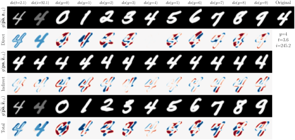
(a) Latent mediator SCM for Morpho-MNIST. Observed variables in the graph: image $(\mathbf{x})$, digit $(y)$, stroke thickness $(t)$ and pixel intensity $(i)$.

Figure 3: Morpho-MNIST counterfactuals from our latent mediator SCM. Direct, indirect and total causal effects of interventions are shown (red: increase; blue: decrease). Recall that $\widetilde{\mathbf{x}}_{\mathrm{IE}}\sim g(\mathbf{pa}_{\mathbf{x}},\widetilde{\mathbf{z}}_{1:L})$ are cross-world counterfactuals, i.e. the potential outcome of $\mathbf{x}$ given $\mathbf{pa}_{\mathbf{x}}$ and the (counterfactual) mediator we would have observed $\widetilde{\mathbf{z}}_{1:L}$ had $\mathbf{pa}_{\mathbf{x}}$ been $\widetilde{\mathbf{pa}}_{\mathbf{x}}$.

Constrained Counterfactual Training.

One issue with fine-tuning $\mathbf{x}$’s HVAE mechanism with counterfactual training is that the original performance on observational data can deteriorate as we update $\{\hat{\theta},\hat{\phi}\}$. To mitigate this, we propose to reframe counterfactual training as a Lagrangian optimization problem, using the differential multiplier method (Platt & Barr, 1987). Our proposed constraint is the pre-trained HVAE’s negative ELBO (free energy $\mathcal{F}_{\mathrm{FE}}$) averaged over the observational data: $c\coloneqq\mathbb{E}_{p_{\mathrm{data}}(\mathbf{x},\mathbf{pa}_{\mathbf{x}})}[\mathcal{F}_{\mathrm{FE}}(\hat{\theta},\hat{\phi};\mathbf{x},\mathbf{pa}_{\mathbf{x}})]$, which should not increase during counterfactual training. Formally, the constrained counterfactual optimization problem is

$$\operatorname*{arg\,min}_{\theta,\phi} \ \mathbb{E}_{p_{\mathrm{data}}(\mathbf{x},\mathbf{pa}_{\mathbf{x}})}\left[\mathcal{L}_{\mathrm{CT}}(\mathcal{M};\mathbf{x},\mathbf{pa}_{\mathbf{x}})\right]$$ (24)

$$\mathrm{s.t.} \ \mathcal{F}_{\mathrm{FE}}(\theta,\phi;\mathbf{x},\mathbf{pa}_{\mathbf{x}})\leq c,$$ (25)

rewritten as the Lagrangian: $\mathcal{L}_{\mathrm{Lg}}(\theta,\phi,\lambda;\mathbf{x},\mathbf{pa}_{\mathbf{x}})=$

$$\mathcal{L}_{\mathrm{CT}}(\mathcal{M};\mathbf{x},\mathbf{pa}_{\mathbf{x}})-\lambda(c-\mathcal{F}_{\mathrm{FE}}(\theta,\phi;\mathbf{x},\mathbf{pa}_{\mathbf{x}})).$$ (26)

Optimizing this Lagrangian involves performing gradient descent on the HVAE’s parameters $\theta$ and $\phi$, and gradient ascent on the Lagrange multiplier $\lambda$. The intended effect is to fine-tune $\mathbf{x}$’s HVAE mechanism to improve counterfactual conditioning by maximizing $I(\widetilde{\mathbf{pa}}_{k};\widetilde{\mathbf{x}})$, without degrading the original performance on observational data.

Table 1: Quantitative evaluation of generated counterfactuals for the Morpho-MNIST test set. Identical learned SCM mechanisms for $t$, $i$, and $y$ are used in all cases to enable direct comparison of causal mechanisms for $\mathbf{x}$. ‘Baseline’ refers to the original DSCM (Pawlowski et al., 2020), $\text{EXO}_{\text{DE}}$ denotes our exogenous prior HVAE, whereas $\text{MED}_{\text{DE}}$ and $\text{MED}_{\text{TE}}$ refer to direct and total effect counterfactuals from our latent mediator model respectively. ‘bpd’ denotes bits per dimension, i.e distortion of null-interventions plus the rate ($D_{\text{KL}}(q\parallel p)$). ‘$\sim$ Prior’ denotes random samples from the model directly above. Accompanying table reporting standard deviations of multiple runs and extra ablations are shown in Appendix C.

			Thickness $(t)$ MAE $\downarrow$				Intensity $(i)$ MAE $\downarrow$				Digit $(y)$ Acc. (%) $\uparrow$
Method	$\beta$	bpd $\downarrow$	$do(t)$	$do(i)$	$do(y)$	mix	$do(t)$	$do(i)$	$do(y)$	mix	$do(t)$	$do(i)$	$do(y)$	mix
Baseline	1	2.04	.112	.178	.175	.177	8.31	8.10	10.4	9.61	99.20	99.08	83.18	89.54
$\sim$ Prior	1	N/A	.193	.225	.191	.209	10.5	11.1	10.6	10.8	82.75	81.10	82.62	81.99
Baseline	3	2.17	.126	.185	.149	.171	14.1	15.5	15.1	15.6	99.47	99.34	97.89	98.34
$\text{EXO}_{\text{DE}}$	1	.674	.125	.140	.149	.148	1.78	2.08	1.87	2.24	99.31	98.88	99.49	99.23
$\sim$ Prior	1	N/A	.178	.192	.175	.186	2.18	3.08	2.20	2.74	98.30	97.68	98.49	97.95
$\text{EXO}_{\text{DE}}$	3	.942	.129	.133	.142	.139	1.83	2.70	1.77	2.32	99.46	99.01	99.73	99.34
$\text{MED}_{\text{DE}}$	1	.682	.125	.137	.157	.149	1.65	1.48	1.80	1.89	99.38	98.73	99.47	99.09
$\text{MED}_{\text{TE}}$	1	.682	.141	.153	.146	.150	1.72	2.17	1.78	2.01	99.75	99.30	99.68	99.41
$\text{MED}_{\text{DE}}$	3	.941	.133	.146	.139	.145	1.94	2.71	1.94	2.45	99.45	99.15	99.62	99.40
$\text{MED}_{\text{TE}}$	3	.941	.130	.141	.135	.138	2.10	3.11	2.13	2.69	99.85	99.65	99.79	99.71

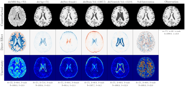
(a) Deep SCM for UK Biobank. MRI Seq. $(m)$, age $(a)$, sex $(s)$, brain $(b)$ & ventricle $(v)$ volume.

Figure 4: Brain MRI counterfactuals from our deep SCM. Direct causal effect is shown (red: increase; blue: decrease). We observe qualitatively sharp $192{\times}192$ counterfactuals that manifest localized interventional changes according to the associated causal graph in (a), whilst preserving the identity of the observation. Counterfactual uncertainty is also shown.

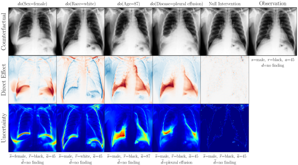
(a) Deep SCM for MIMIC-CXR. The variables in the causal graph are: age $(a)$, sex $(s)$, race $(r)$, disease $(d)$ and chest x-ray $(\mathbf{x})$. The disease $d$ is pleural effusion.

Figure 5: Chest X-ray counterfactuals from our deep SCM. Direct causal effect is shown (red: increase; blue: decrease). We observe qualitatively sharp $192{\times}192$ counterfactuals that manifest localized interventional changes according to the associated causal graph in (a), whilst preserving the identity of the observation. Counterfactual uncertainty is also shown.

4 Experiments

We present 3 case studies on counterfactual inference of high-dimensional structured variables. To quantitatively evaluate our deep SCMs, we measure effectiveness and composition, which are axiomatic properties of counterfactuals that hold true in all causal models (Pearl, 2009; Monteiro et al., 2023). Effectiveness is measured via the anticausal parent predictors from Section 3.4, and composition is measured via the distortion of $\mathbf{x}$’s HVAE mechanism upon null-interventions. Please refer to Appendix B for more details.

4.1 Causal Mediation on Morpho-MNIST

Causal mediation studies the extent to which the effect of a treatment is mediated by another variable in order to help explain why/how individuals respond to certain stimulus (Imai et al., 2010). To demonstrate this concept on structured variables, we extend the causal modelling scenario presented by Pawlowski et al. (2020) using the Morpho-MNIST (Castro et al., 2019) dataset. The dataset is generated from a known causal graph shown in Figure 3(a) and Appendix C, where we introduced an additional digit class variable $y$ to study discrete counterfactuals. We use normalizing flows to model the causal mechanisms of variables $t$, $i$ and $y$ as in Appendix A.1, and use the proposed HVAE-based mechanisms for $\mathbf{x}$. Figure 3(a) demonstrates our latent mediator model’s ability to estimate the direct, indirect and total causal effects of interventions. Notably, direct effect counterfactuals preserve the identity and modify only the parents $\mathbf{pa}_{\mathbf{x}}$, whereas indirect effect (cross-world) counterfactuals preserve $\mathbf{pa}_{\mathbf{x}}$ whilst changing the style according to the counterfactual mediator $\widetilde{\mathbf{z}}_{1:L}$ we would have observed had $\mathbf{pa}_{\mathbf{x}}$ been $\widetilde{\mathbf{pa}}_{\mathbf{x}}$. Our total effect counterfactuals are a combination of direct and indirect effects, which agrees with causal mediation theory (Robins & Greenland, 1992; Pearl, 2001).

Since the generative process is known, we can measure the quality of our counterfactual approximations using the ground truth mechanisms. For variable $y$, we used an accurate digit classifier with ${\simeq}99.5\%$ test acc. instead. Table 1 reports counterfactual evaluation results from random interventions on each parent. We find that our exogenous prior and latent mediator HVAE $\mathbf{x}$ mechanisms perform similarly, and both outperform baselines (Pawlowski et al., 2020) by a wide margin especially on digit (discrete) counterfactuals which are more challenging. Total effect counterfactuals ($\text{MED}_{\text{TE}}$) are generally more faithful to counterfactual conditioning than direct effect counterparts ($\text{MED}_{\text{DE}}$) but are more likely to deviate from the identity of observations.

4.2 Brain Imaging Counterfactuals

To demonstrate our model’s ability to produce faithful high-fidelity counterfactuals of real data, we extend our approach to a real-world scenario involving brain MRI scans from the UK Biobank (Sudlow et al., 2015). As before, we start with an assumed causal generative process involving a set of observed variables as shown in Figure 4(a). The causal graph is medically informed and extends the scenario in Pawlowski et al. (2020) by: (i) introducing an additional MRI Sequence (T1/T2) binary variable $m$ to enable discrete counterfactuals; (ii) having $s\rightarrow\mathbf{x}$ directly. We used a scaled-up version of our exogenous prior HVAE as $\mathbf{x}$’s mechanism and used (conditional) normalizing flows for the other mechanisms (see Appendix A.1). As shown in Figure 4, our deep SCM is capable of producing qualitatively sharp $192{\times}192$ counterfactuals with localised changes according to the intervened upon parent(s) and the associated causal graph. Importantly, the identity of subjects is well preserved in all cases including null-interventions (i.e. $do(\cdot)$ nothing). Table 2 shows the counterfactual effectiveness results from random interventions on each variable. We observed satisfactory initial counterfactual effectiveness and significant improvements of post counterfactual training, demonstrating the merit of the proposed approach. Please refer to Appendix A.2 for notes on abduction uncertainty and D for additional results.

4.3 Chest X-ray Imaging Counterfactuals

We further extend the proposed approach to the MIMIC-CXR dataset (Johnson et al., 2019) to demonstrate our model’s ability to estimate high-fidelity counterfactuals of real chest X-ray images. This is motivated by the need for a better understanding of algorithmic bias and reported subgroup disparities (Bernhardt et al., 2022). We begin with an assumed causal generative process of data involving the following observed variables: age ($a$), sex ($s$), race ($r$), disease ($d$), and chest X-ray image ($\mathbf{x}$). Notably, we assume that age $a$ causes disease $d$ (pleural effusion) which requires inference of discrete counterfactuals from upstream interventions on age. For details on computing discrete counterfactuals and other experiments, please refer to Appendix E. Following the general setup in Section 4.2, we used a scaled-up version of our exogenous prior HVAE for $\mathbf{x}$’s mechanism. We trained for relatively few iterations on MIMIC-CXR; ${\simeq}210$K. The quantitative counterfactual evaluation results from random interventions on each variable are reported in Table 2. We observed significant improvements in counterfactual effectiveness post counterfactual training, particularly for race, age and disease attributes. For extensive visual evaluation results please refer to Appendix E.4.

Table 2: Quantitative evaluation of generated test set counterfactuals for UK Biobank (Top) and MIMIC-CXR (Bottom). Random interventions on each variable were performed and counterfactual effectiveness was measured via attribute predictors. ‘mixed’ denotes also randomizing the intervened upon variable. Results in brackets $(\uparrow\cdot),(\downarrow\cdot)$ are the absolute differences in effectiveness between regular training and with fine-tuning $\mathbf{x}$’s mechanism using counterfactual training (see Appendix F).

Intervention	Sex $(s)$	MRI $(m)$	Age $(a)$	Brain Vol. $(b)$	Ventricle Vol. $(v)$
(UK Biobank)	ROCAUC $\uparrow$	ROCAUC $\uparrow$	MAE (years) $\downarrow$	MAE (ml) $\downarrow$	MAE (ml) $\downarrow$
$do(s)$	0.9905 ($\uparrow$ 0.172)	1.0 (-)	4.849 ($\downarrow$ 0.018)	24.55 ($\downarrow$ 24.5)	1.854 ($\downarrow$ 0.322)
$do(m)$	0.9893 ($\uparrow$ 0.023)	1.0 (-)	4.846 (-)	26.14 ($\downarrow$ 1.88)	1.932 ($\downarrow$ 0.092)
$do(a)$	0.9892 ($\uparrow$ 0.016)	1.0 (-)	4.937 ($\uparrow$ 0.004)	26.24 ($\downarrow$ 7.31)	1.890 ($\downarrow$ 0.451)
$do(b)$	0.9944 ($\uparrow$ 0.069)	1.0 (-)	5.059 ($\downarrow$ 0.032)	25.49 ($\downarrow$ 38.6)	1.846 ($\downarrow$ 0.933)
$do(v)$	0.9893 ($\uparrow$ 0.031)	1.0 (-)	6.045 ($\downarrow$ 0.102)	25.69 ($\downarrow$ 3.22)	1.826 ($\downarrow$ 2.115)
mixed	0.9899 ($\uparrow$ 0.061)	1.0 (-)	5.128 ($\downarrow$ 0.046)	25.41 ($\downarrow$ 15.1)	1.900 ($\downarrow$ 0.822)

Intervention	Sex $(s)$	Race $(r)$	Age $(a)$	Disease $(d)$
(MIMIC-CXR)	ROCAUC $\uparrow$	ROCAUC $\uparrow$	MAE (years) $\downarrow$	ROCAUC $\uparrow$
$do(s)$	1.000 ($\uparrow$0.078)	0.839 ($\uparrow$0.094)	6.485 ($\downarrow$0.198)	0.969 ($\uparrow$0.038)
$do(r)$	0.997 ($\uparrow$0.002)	0.867 ($\uparrow$0.283)	6.311 ($\downarrow$0.115)	0.874 ($\uparrow$0.008)
$do(a)$	0.997 ($\uparrow$0.002)	0.807 ($\uparrow$0.058)	6.643 ($\downarrow$3.426)	0.916 ($\uparrow$0.033)
$do(d)$	0.997 ($\uparrow$0.001)	0.793 ($\uparrow$0.041)	6.568 ($\downarrow$0.189)	0.982 ($\uparrow$0.258)
mixed	0.998 ($\uparrow$0.015)	0.828 ($\uparrow$0.116)	6.497 ($\downarrow$0.866)	0.950 ($\uparrow$0.076)

5 Related Work

Our work bolsters an ongoing effort to combine representation learning and causality (Bengio et al., 2013; Schölkopf et al., 2021). Causal representation learning is also closely linked to disentanglement, where the goal is to uncover the true underlying (disentangled) generative factors of data (Higgins et al., 2017; Locatello et al., 2019; Kim & Mnih, 2018; Chen et al., 2018). Generative models such as VAEs (Kingma & Welling, 2013), GANs (Goodfellow et al., 2020), Normalizing Flows (Tabak & Vanden-Eijnden, 2010; Rezende & Mohamed, 2015) and Diffusion models (Sohl-Dickstein et al., 2015; Ho et al., 2020; Song et al., 2021b) have become indispensable tools for causal representation learning. They have been leveraged for causal effect estimation (Louizos et al., 2017; Kocaoglu et al., 2017; Tran & Blei, 2017), causal discovery (Yang et al., 2021; Sanchez et al., 2022b; Geffner et al., 2022), and various other extensions have enabled modelling of conditional (Trippe & Turner, 2018; Mirza & Osindero, 2014; Sohn et al., 2015; Dhariwal & Nichol, 2021) and interventional distributions (Kocaoglu et al., 2018; Ke et al., 2019; Xia et al., 2021; Zečević et al., 2021). However, few works have focused on fulfilling all three rungs of Pearl’s ladder of causation: (i) association; (ii) intervention; (iii) counterfactuals (Pearl, 2009; Bareinboim et al., 2022) in a principled manner using deep models.

Our work is most closely related to DSCMs (Pawlowski et al., 2020) and NCMs (Xia et al., 2021, 2023) in that we leverage deep learning components to learn causal mechanisms. However, our focus is on the practical estimation and evaluation of plausible high-fidelity image counterfactuals, whereas previous work mostly focused on theoretical and/or proof-of-concept low-resolution settings. Sanchez & Tsaftaris (2021); Sanchez et al. (2022a) proposed Diffusion SCMs (Diff-SCMs) for high-fidelity counterfactuals, but considered only two-variable causal models. Our approach is inspired by recent identifiability results in deep generative models (Khemakhem et al., 2020; Hyvarinen et al., 2019), as well as modern HVAE architectures (Vahdat & Kautz, 2020; Child, 2020) which are readily amenable to explicit, identity-preserving abduction. Causal mediation analysis concepts like direct, indirect and total effects (Robins & Greenland, 1992; Imai et al., 2010; Pearl, 2001) also guided our latent mediator SCM setup. Many image-to-image translation approaches (Isola et al., 2017; Liu et al., 2017; Su et al., 2022; Saharia et al., 2022; Brooks et al., 2022; Preechakul et al., 2022) are also related to counterfactual inference, but only in an informal sense as they do not explicitly perform abduction, model interventions, nor use causal structure.

6 Conclusion

We present a pragmatic causal generative modelling framework for estimating high-fidelity image counterfactuals using deep SCMs. Our proposed deep causal mechanisms are inspired by recent identifiability results for deep generative models, as well as causal mediation analysis theory. We show how to plausibly estimate direct, indirect, and total causal effects on high-dimensional structured variables such as images, and provide abduction uncertainty estimates. We quantify the soundness of our counterfactuals by evaluating axiomatic properties that hold true in all causal models: i.e. effectiveness and composition. We believe the ability to generate plausible counterfactuals could greatly benefit several important areas: (i) explainability, e.g. through causal mediation effects as studied here; (ii) data augmentation, e.g. mitigating data scarcity and underrepresentation of subgroups; (iii) robustness, to e.g. spurious correlations. Our work contributes primarily to the empirical and theoretical advancement of counterfactual inference models – valuable extensions for future work include demonstrating the advantage of using counterfactuals in the aforementioned areas.

Limitations.

This work considers only Markovian SCMs, wherein all causal effects are identifiable from observed data under the assumption of no unobserved confounding. Markovianity is a common assumption in academic literature but may be too restrictive in some real-world scenarios. We take a pragmatic empirical approach to counterfactual evaluation by measuring their axiomatic soundness rather than being bound by a lack of theoretical identifiability in the limit of infinite data. Nonetheless, extensions to Semi- and/or Non-Markovian settings would boost the practicality of our approach, but this is highly non-trivial for structured variables. Further, we stress that any conclusions drawn using our approach are strictly dependent on the correctness of the assumed SCM. We urge practitioners to carefully consider the ethical implications of their modelling assumptions when applying this framework in real-world settings.

Acknowledgements.

This project has received funding from the ERC under the EU’s Horizon 2020 research and innovation programme (grant No. 757173). B.G. is grateful for the support from the Royal Academy of Engineering as part of his Kheiron Medical Technologies / RAEng Research Chair in Safe Deployment of Medical Imaging AI.

(a) With $q(\cdot)$ correction

(b) Without $q(\cdot)$ correction

Figure 6: Conditional HVAE generative model structures for the proposed latent mediator model. The associated inference model is the same as in Figure 1(a). (a) Like the ladder VAE (Sønderby et al., 2016), each conditional prior distribution $p_{\theta}(\mathbf{z}_{i}\mid\mathbf{z}_{>i})$ at each layer $i$ is corrected by a data-dependent likelihood contribution from the posterior of the layer above via $\mathbf{h}_{i+1}$. Unlike (a), the conditional prior distributions at each layer of (b) do not depend on the posterior, but each posterior still depends on the prior from the layer above.

Appendix A Supplementary Methods

A.1 Invertible Mechanisms for Attributes

Attributes which are ancestors of the image $\mathbf{x}$, $\mathbf{an}_{\mathbf{x}}=\{a_{1},\dots,a_{N-1}\}\supseteq\mathbf{pa}_{\mathbf{x}}$, are generally not assumed to be independent, so we learn their structural assignments from data. To enable tractable abduction for $\mathbf{an}_{\mathbf{x}}$, we learn invertible mechanisms $f_{k}$ using conditional normalizing flows (Trippe & Turner, 2018) as suggested by Pawlowski et al. (2020). Each attribute’s mechanism $a_{k}\coloneqq f_{k}(u_{k};\mathbf{pa}_{k})$ is a conditional flow, where $a_{k}$ is expressed as a parameterised function of $\mathbf{pa}_{k}$ and samples from a base distribution $u_{k}\sim p_{u}(u_{k})$. The conditional density is given by

$$p(a_{k}\mid\mathbf{pa}_{k})=p_{u}(u_{k})\left|\mathrm{det}J_{f_{k}}(u_{k})\right|^{-1},$$ (27)

where $u_{k}=f_{k}^{-1}(a_{k};\mathbf{pa}_{k})$, and $J_{f_{k}}(u_{k})$ is the Jacobian matrix of all partial derivatives of $f_{k}$ with respect to $u_{k}$. The base distribution for the exogenous noise is typically assumed to be Gaussian, which may be restrictive. Moreover, we note that $u_{k}$ here is not strictly latent (unobserved) as described in SCM theory, since knowing $(a_{k},\mathbf{pa}_{k})$ uniquely determines $u_{k}$. A counterfactual attribute $\widetilde{a}_{k}$ is given by forwarding the mechanism using its counterfactual parents and the abducted exogenous noise: $\widetilde{a}_{k}\coloneqq f_{k}(u_{k};\widetilde{\mathbf{pa}}_{k})$. In practice, we use standard Gaussians as base distributions for the exogenous noise and leverage available PyTorch (Paszke et al., 2019) & Pyro (Bingham et al., 2019) implementations.

Figure 7: Showing a (1 stochastic layer) VAE collapsing to a deterministic AE throughout training on Morpho-MNIST (3 random seeds used). We observe that the marginal posterior scale tends towards zero when the image (Gaussian) likelihood scale is fixed in the near-deterministic regime. This observation is consistent with the VAE self-consistency claims of Nielsen et al. (2020) and Reizinger et al. (2022).

A.2 Distribution over Causal Worlds

As explained in Section 3.1, the original DSCM (Pawlowski et al., 2020) framework’s VAE-based causal mechanism for $\mathbf{x}$ was trained in the near-deterministic regime, thereby incidentally attempting to deterministically abduct $\mathbf{x}$’s exogenous like a normalizing flow. Consequently, the model struggled to: (i) produce realistic random samples from the SCM; (ii) represent abduction uncertainty; (iii) induce a distribution over causal worlds. Our proposed HVAE-based deep causal mechanisms address these issues.

The counterfactual distribution of $\widetilde{\mathbf{x}}$: $P_{\mathcal{M}}(\widetilde{\mathbf{x}}\mid do(\widetilde{\mathbf{pa}}_{k}),\mathbf{x})$, is our distribution of interest associated with the modified probabilistic SCM $\langle\mathcal{M}_{do(\widetilde{\mathbf{pa}}_{k})},P(U|X)\rangle$, after the three-step procedure (Section 2.1). The prior and posterior distributions over the exogenous noise variables (with an exogenous prior HVAE mechanism for $\mathbf{x}$) are given by

$$P(U) =\underbrace{p_{\theta}(\mathbf{z}_{1:L})p(\boldsymbol{\epsilon})}_{p(\mathbf{u}_{\mathbf{x}})}\prod_{i=1}^{N-1}p(\mathbf{u}_{i}),$$ (28)

$$P(U|X) \approx\underbrace{q_{\phi}(\mathbf{z}_{1:L}\mid\mathbf{x},\mathbf{pa}_{\mathbf{x}})\delta(\boldsymbol{\epsilon}\mid\mathbf{x},\mathbf{pa}_{\mathbf{x}})}_{\approx p(\mathbf{u}_{\mathbf{x}}\mid\mathbf{x},\mathbf{pa}_{\mathbf{x}})}\prod_{i=1}^{N-1}\delta(\mathbf{u}_{i}\mid a_{i},\mathbf{pa}_{i}).$$ (29)

Since abduction is non-deterministic in this model, we can sample different realizations of the exogenous variables from $P(U|X)$ by sampling from the HVAE encoder $q_{\phi}(\mathbf{z}_{1:L}|\mathbf{x},\mathbf{pa}_{\mathbf{x}})$, thereby inducing a distribution over causal worlds and yielding varied counterfactuals of $\mathbf{x}$. Note that the Delta distributed $\delta(\cdot)$ exogenous variable posteriors are a result of deterministic abduction (e.g. from inverting a normalizing flow mechanism). Furthermore, we can calculate the first and second moments of the counterfactual distribution:

$$\boldsymbol{\mu}_{\widetilde{\mathbf{x}}}=\mathbb{E}_{P(U|X)}\big{[}P_{\mathcal{M}}(\widetilde{\mathbf{x}}\mid do(\widetilde{\mathbf{pa}}_{k}),\mathbf{x})\big{]},\quad \boldsymbol{\sigma}_{\widetilde{\mathbf{x}}}=\mathrm{Var}_{P(U|X)}\big{[}P_{\mathcal{M}}(\widetilde{\mathbf{x}}\mid do(\widetilde{\mathbf{pa}}_{k}),\mathbf{x})\big{]}^{\frac{1}{2}},$$ (30)

where $\boldsymbol{\mu}_{\widetilde{\mathbf{x}}}$ can be interpreted as the most likely counterfactual of $\mathbf{x}$ and $\boldsymbol{\sigma}_{\widetilde{\mathbf{x}}}$ as a measure of counterfactual uncertainty.

A.3 Latent Mediator Architectures

As shown in Figure 6(b), we can alter the conditional generative model structure of the latent mediator model, such that the conditional prior distributions no longer receive data-dependent corrections from previous layer posteriors as in the Ladder VAE (Sønderby et al., 2016). We find that this architecture (Figure 6(b)) is less prone to ignored counterfactual conditioning, especially when trained with parent conditioning dropout (see comparative results in Table 3). Parent conditioning dropout consists of randomly selecting when $\mathbf{pa}_{\mathbf{x}}$ is merged into the downstream. We can either drop the $\mathbf{pa}_{\mathbf{x}}$ merge connections between each $\mathbf{h}_{i}$ and $\mathbf{z}_{i}$ (deterministic path) or between each $\mathbf{z}_{i}$ and $\mathbf{z}_{i-1}$ (stochastic path), whilst holding the other fixed. Parent conditioning dropout is somewhat reminiscent of classifier-free guidance (Ho & Salimans, 2022) in diffusion models but the application and motivations here are different; to prevent the model from prioritising one conditioning path over the other and improve counterfactual conditioning on $\widetilde{\mathbf{pa}}_{\mathbf{x}}$ in the forward model with the abducted noise $\mathbf{z}_{1:L}$ fixed.

Table 3: Comparing counterfactual effectiveness of random interventions using our latent mediator model ($\beta{=}1$) when trained with and without conditioning dropout (CD) as described in Section A.3. We find that effectiveness of digit counterfactuals improves significantly with CD at the cost of slightly worse composition (higher bits per dimension).

			Thickness $(t)$ MAE $\downarrow$				Intensity $(i)$ MAE $\downarrow$				Digit $(y)$ Acc. (%) $\uparrow$
Method	CD	bpd $\downarrow$	$do(t)$	$do(i)$	$do(y)$	mix	$do(t)$	$do(i)$	$do(y)$	mix	$do(t)$	$do(i)$	$do(y)$	mix
$\text{MED}_{\text{DE}}$	N	.676	.127	.133	.252	.202	1.70	2.04	1.85	2.17	99.30	99.06	81.07	88.37
$\text{MED}_{\text{TE}}$	N	.676	.162	.168	.225	.200	1.73	2.60	1.79	2.22	99.74	99.36	94.28	95.87
$\text{MED}_{\text{DE}}$	Y	.682	.125	.137	.157	.149	1.65	1.48	1.80	1.89	99.38	98.73	99.47	99.09
$\text{MED}_{\text{TE}}$	Y	.682	.141	.153	.146	.150	1.72	2.17	1.78	2.01	99.75	99.30	99.68	99.41

Appendix B Axiomatic Counterfactual Evaluation

In order to quantitatively evaluate our approximate counterfactual inference models, we measure the axiomatic properties of counterfactuals: (i) composition; (ii) effectiveness; (iii) reversibility (Pearl, 2009; Monteiro et al., 2023), which hold true in all causal models. The soundness (Galles & Pearl, 1998) and completeness (Halpern, 1998) theorems state that composition, effectiveness and reversibility are the necessary and sufficient properties of counterfactuals in any causal model. The three axiomatic properties of counterfactuals can be summarised as follows:

1. Composition: Intervening on a variable to have a value it would have had without our intervention will not affect the other variables in the system;

2. Effectiveness: Intervening on a variable to have a specific value will cause the variable to take on that value;

3. Reversibility: Precludes multiple solutions due to feedback loops, and follows directly from composition in recursive systems such as DAGs. Refer for (Pearl, 2009) for further details on non-recursive systems.

Following the counterfactual evaluation framework proposed by Monteiro et al. (2023), we measure counterfactual effectiveness using a ‘pseudo-oracle’ function’s accuracy/error (i.e. calculated from our parent predictors) and measure composition via the distortion induced by $\mathbf{x}$’s mechanism from (repeated) null-interventions. In the case of a HVAE-based causal mechanism for $\mathbf{x}$, composition can be understood as reconstructing the input given observed parents, and reversibility as the act of cycling back between factual and counterfactual parent interventions. In both cases, distance metrics can be used to measure differences between counterfactual and factual images (e.g. $L1$ image distance per-pixel).

Figure 8: Evidence lower bound, distortion and rate throughout training on Morpho-MNIST (shown in nats per dimension). Top row corresponds to our exogenous prior HVAE, and the bottom row to the HVAE for our latent mediator model. Identical architectures were used in both cases, leading to similar results despite the change in conditioning structure. Dashed and solid lines correspond to training and validation respectively.

Figure 9: Rate-distortion curves for our exogenous prior HVAE (Top) and the latent mediator model’s HVAE (Bottom) trained on Morpho-MNIST (shown in nats per dimension). For both models, we can see that increasing $\beta$ reduces the rate whilst increasing distortion, encouraging the model to ignore imperceptible details and focus more on semantic compression. This helps explain why increasing $\beta$ can improve counterfactual conditioning, since the model is discouraged from focusing mostly on improving distortion (image likelihood) and finding a solution $p_{\theta}(\mathbf{x})=p_{\theta}(\mathbf{x}|c)$ by ignoring conditioning $c$.

Table 4: Additional quantitative evaluation of generated counterfactuals for the Morpho-MNIST test set. Supplementary to Table 1 in the main text and includes further ablations on the $\beta$ penalty used during training.

			Thickness $(t)$ MAE $\downarrow$				Intensity $(i)$ MAE $\downarrow$				Digit $(y)$ Acc. (%) $\uparrow$
Method	$\beta$	bpd $\downarrow$	$do(t)$	$do(i)$	$do(y)$	mix	$do(t)$	$do(i)$	$do(y)$	mix	$do(t)$	$do(i)$	$do(y)$	mix
Baseline	3	2.17	.126	.185	.149	.171	14.1	15.5	15.1	15.6	99.47	99.34	97.89	98.34
$\sim$ Prior	3	N/A	.174	.222	.173	.201	15.4	17.1	15.3	16.4	96.21	96.01	96.39	96.27
$\text{EXO}_{\text{DE}}$	5	1.08	.137	.158	.137	.149	2.91	4.09	2.82	3.59	99.62	99.28	99.82	99.49
$\text{MED}_{\text{DE}}$	5	1.07	.139	.149	.140	.145	2.66	4.28	2.61	3.57	99.61	99.26	99.76	99.52
$\text{MED}_{\text{TE}}$	5	1.07	.126	.141	.127	.134	2.96	4.87	2.94	4.04	99.86	99.60	99.82	99.66

Table 5: Quantitative evaluation of generated counterfactuals for the Morpho-MNIST test set. Sister table of results in Tables 1 & 4 in the main text reporting the standard deviations of results from three random seed runs.

			Thickness $(t)$ MAE $\downarrow$				Intensity $(i)$ MAE $\downarrow$				Digit $(y)$ Acc. (%) $\uparrow$
Method	$\beta$	bpd $\downarrow$	$do(t)$	$do(i)$	$do(y)$	mix	$do(t)$	$do(i)$	$do(y)$	mix	$do(t)$	$do(i)$	$do(y)$	mix
Baseline	1	2.04	1e-3	1e-3	2e-3	1e-3	1e-3	2e-2	3e-2	4e-3	4e-4	8e-4	7e-4	2e-3
$\sim$ Prior	1	N/A	3e-3	5e-4	1e-3	2e-3	5e-2	3e-2	9e-3	1e-2	3e-3	2e-3	3e-3	3e-3
Baseline	3	2.17	2e-3	1e-3	8e-4	1e-3	4e-2	1e-2	8e-2	0.13	6e-4	5e-4	1e-3	1e-3
$\sim$ Prior	3	N/A	9e-4	1e-3	2e-3	1e-3	3e-2	0.146	6e-2	0.122	1e-3	5e-5	1e-3	1e-3
$\text{EXO}_{\text{DE}}$	1	.674	9e-4	2e-4	6e-4	2e-3	2e-2	3e-2	1e-2	4e-2	5e-4	5e-4	3e-4	3e-4
$\sim$ Prior	1	N/A	2e-3	9e-4	2e-3	8e-5	1e-2	3e-2	1e-2	9e-3	3e-4	1e-3	1e-3	3e-4
$\text{EXO}_{\text{DE}}$	3	.942	1e-3	1e-3	2e-4	2e-3	1e-2	4e-2	6e-3	1e-2	1e-4	6e-4	3e-4	1e-3
$\text{MED}_{\text{DE}}$	1	.682	6e-4	4e-5	1e-3	2e-3	2e-2	2e-2	1e-2	3e-4	3e-4	6e-4	4e-5	3e-4
$\text{MED}_{\text{TE}}$	1	.682	2e-4	6e-4	1e-3	7e-4	2e-2	1e-2	5e-3	3e-3	4e-4	5e-4	4e-4	3e-4
$\text{MED}_{\text{DE}}$	3	.941	8e-4	2e-4	1e-3	4e-4	9e-3	2e-2	9e-3	3e-2	1e-4	2e-4	8e-4	2e-4
$\text{MED}_{\text{TE}}$	3	.941	3e-4	8e-4	9e-4	2e-3	1e-2	4e-2	3e-2	4e-2	4e-4	1e-3	6e-4	1e-3

Appendix C Morpho-MNIST

C.1 Dataset Details

For our Morpho-MNIST experiments, we construct a similar scenario to Pawlowski et al. (2020) in which a dataset is generated according to the following known structural causal model:

$$y \coloneqq f_{y}(u_{y}),\qquad u_{y}\sim\text{MNIST}$$ (31)

$$t \coloneqq f_{t}(u_{t})=0.5+u_{t},\qquad u_{t}\sim\mathrm{Gamma}(10,5)$$ (32)

$$i \coloneqq f_{i}(t,u_{i})=191\cdot\sigma(0.5u_{i}+2t-5),\qquad u_{i}\sim\mathcal{N}(0,1)$$ (33)

$$\mathbf{x} \coloneqq f_{x}(i,t,y,u_{x})=\text{Set}_{i}(i,y,\text{Set}_{t}(t,y,u_{x})),\qquad u_{x}\sim\text{MNIST},$$ (34)

The $\text{Set}_{i}(\cdot)$ and $\text{Set}_{t}(\cdot)$ are morphological operations that act on an image and set its intensity $i$ and thickness $t$. We’ve introduced the categorical variable $y$ for digit class, to increase the complexity of the learning problem and extend counterfactual inference to the discrete case. The resulting dataset follows the original MNIST dataset splits.

C.2 Experiment Setup

Our deep SCMs are implemented in Pyro and Pytorch. Unlike Pawlowski et al. (2020), we train the causal mechanisms (normalizing flows) for all variables except the image $\mathbf{x}$ concurrently in Pyro, whereas $\mathbf{x}$’s causal mechanism is trained separately in Pytorch. Training $\mathbf{x}$’s HVAE mechanism separately from the flow mechanisms allows us to compare different versions of the $\mathbf{x}$’s mechanism fairly while keeping the rest of the SCM’s mechanisms fixed. Once all the SCM components are trained they are combined into a single PyTorch module for counterfactual training and inference.

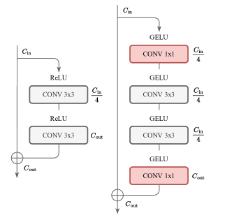
Figure 10: The residual blocks used to build our HVAEs. The block on the RHS tends to perform better but requires more GPU memory to run, so we used the LHS one for the Brain MRI dataset.

Architecture.

For the experiments on the Morpho-MNIST dataset, we built upon the general setup of the very deep VAE (VDVAE) from Child (2020) and introduced structural modifications to accommodate both parent conditioning and abduction in our exogenous prior and latent mediator models described in the text. The architecture itself is largely based on the ResNet-VAE of (Kingma et al., 2016) but contains many more layers of stochastic latent variables. The prior and posterior are diagonal Gaussian distributions and the model is trained end-to-end by optimizing the variational bound on the log-likelihood (ELBO) (Kingma & Welling, 2013; Kingma et al., 2016; Maaløe et al., 2019). Both our exogenous prior and latent mediator HVAEs for Morpho-MNIST have $20$ stochastic latent variables spanning 5 resolution scales up to the $32{\times}32$ input resolution: $\{1^{2},4^{2},8^{2},16^{2},32^{2}\}$. Each resolution scale contains $4$ inverted residual blocks (Figure 10), and each latent variable has $16$ channels. We use variable widths per resolution of: $\{16,32,64,128,256\}$, and the total trainable parameter count is $\simeq$2M. For downsampling we use average pooling layers and for upsampling we use nearest neighbour interpolation followed by convolution. In order to condition our HVAEs, we expand and concatenate $\mathbf{pa}_{\mathbf{x}}$ with the latent variables $\mathbf{z}_{i}$ at each layer of the hierarchy in the locations specified in Figures 1 and 6. The resulting tensor is then merged into the downstream via a $1{\times}1$ convolution.

Training Details.

We trained our HVAEs for $\simeq$1M steps using a batch size of 32 and the AdamW optimizer (Loshchilov & Hutter, 2017). We used an initial learning rate of 1e-3 with 100 linear warmup steps, $\beta_{1}=0.9$, $\beta_{2}=0.9$ and a weight decay of 0.01. We set gradient clipping to 350 and set a gradient update skipping threshold of 500 (based on $L2$ norm). No significant training instability was observed. The final artefact is an exponential moving average of the model parameters with a rate of 0.999 which we use at inference time. For data-augmentation, we applied zero-padding of $4$ on all borders and random cropped to $32{\times}32$ resolution. Pixel intensities we rescaled to $[-1,1]$ for and validation/test images were zero-padded to $32{\times}32$.

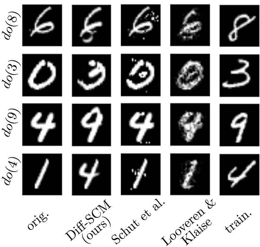
Figure 11: Figure credit belongs solely to Sanchez & Tsaftaris (2021) – reused here for qualitative comparison purposes only. From visual inspection alone, we can observe that the counterfactuals generated from our proposed deep SCM (e.g. see Appendix C.3) are far superior in both counterfactual effectiveness and composition compared to the previous methods shown (Sanchez & Tsaftaris, 2021; Schut et al., 2021; Van Looveren & Klaise, 2021).

C.3 Extra Results

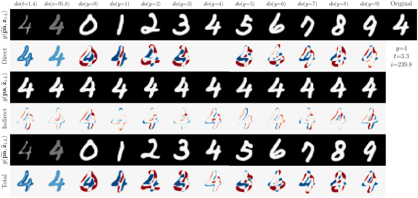
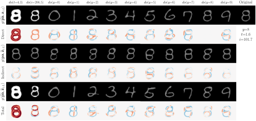
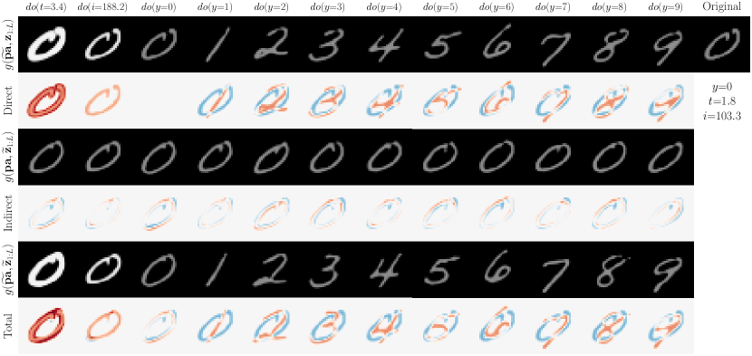
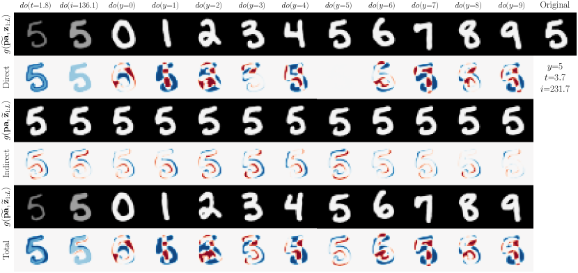
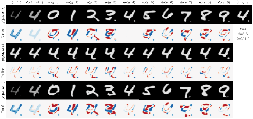
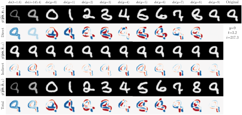
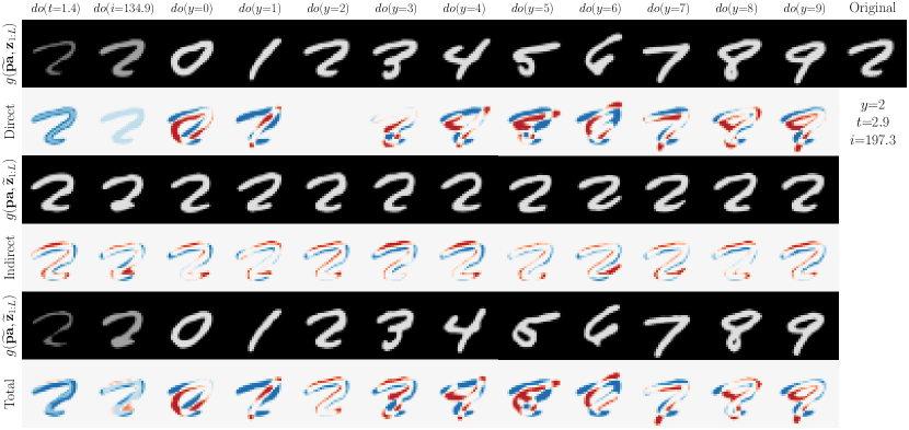
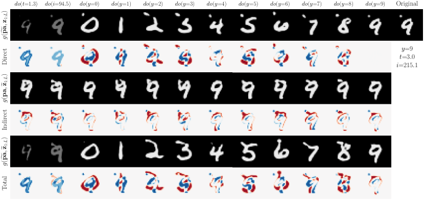
Figure 12: Visualizing additional random Morpho-MNIST test set counterfactuals from our latent mediator model ($\beta{=}1$). Direct, indirect and total effects are also shown. We observe counterfactuals which are faithful to interventions and the associated causal graph (e.g. intervening on thickness causes intensity to increase/decrease.). Intervening on the parents preserves observational identity (e.g. writing style). Recall that cross-world (indirect effect, row(s) 3) counterfactuals $\widetilde{\mathbf{x}}_{\text{IE}}\sim g(\mathbf{pa}_{\mathbf{x}},\widetilde{\mathbf{z}}_{1:L})$ are the outcome of $\mathbf{x}$ given observed $\mathbf{pa}_{\mathbf{x}}$ and the counterfactual mediator we would have observed $\widetilde{\mathbf{z}}_{1:L}$ had $\mathbf{pa}_{\mathbf{x}}$ been $\widetilde{\mathbf{pa}}_{\mathbf{x}}$. We can see that the effect of the parents is mediated by $\mathbf{z}_{1:L}$, which mostly affects the writing style, and changes according to which counterfactual parent caused the (inferred) counterfactual mediator $\widetilde{\mathbf{z}}_{1:L}$.

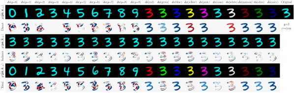
Figure 13: Test set counterfactuals produced by our latent mediator model using the Colour-MNIST dataset from (Monteiro et al., 2023). In this case, the SCM is very simple and consists of only 3 variables: digit $y$, colour $c$ and image $\mathbf{x}$. There are 10 different discrete colours, there is no assumed causal relationship between $y$ & $c$, and both $y$ and $c$ cause $\mathbf{x}$. We can observe clear localised changes based on the intervened upon parent variable whilst the identity of the observation is preserved. There is also no (visible) causal influence from $y$ to $c$ or vice-versa like in the thickness $t$ and intensity $i$ scenario from Morpho-MNIST where $t$ caused $i$. Direct, indirect and total causal effects are also shown.

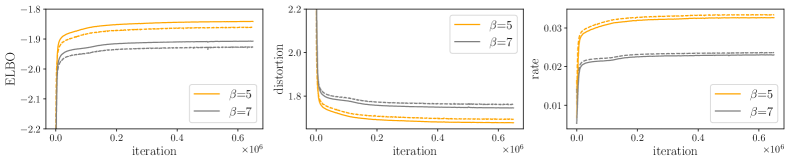
Figure 14: Evidence lower bound, distortion and rate throughout training of our exogenous prior HVAE mechanism on UK Biobank (shown in nats per dimension, top row). Dashed and solid lines correspond to training and validation respectively.

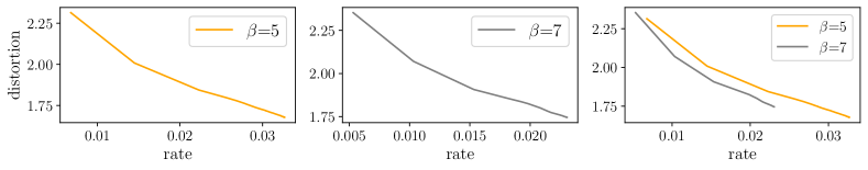
Figure 15: Rate-distortion curves of our exogenous prior HVAE mechanism on UK Biobank. We can again observe higher $\beta$ penalty encourages higher semantic compression, which leads to improvements in counterfactual conditioning (in terms of counterfactual effectiveness) at the cost of worse distortion (counterfactual composition).

Appendix D Brain MRI (UK Biobank)

D.1 Dataset Details

In terms of data generation and pre-processing, we follow the original pipeline used by Alfaro-Almagro et al. (2018) and Pawlowski et al. (2020). The pre-processing entails skull removal, bias field correction, segmentation of brain structures, and registration. Mid-axial 2D slices were then extracted and max-min normalised to $[0,255]$ inside the brain mask, whereas background pixels were set to zero. The attributes for each subject (age, sex, brain/ventricle volume) were retrieved from the UK Biobank dataset. In addition, we use both T1-weighted and T2-FLAIR brain MRI scans (when available) and include a binary indicator variable ($m$) for the scan modality in our structural causal models. We randomly split the full dataset into subsets of 19466 training, 3500 validation and 3500 test samples. Further, we ensure no overlapping subjects between the training and evaluation datasets exist.

D.2 Experiment Setup

Architecture.

For the Brain MRI experiments, we used a scaled-up version of our exogenous prior HVAE for $\mathbf{x}$’s mechanism to accommodate the higher resolution of $192{\times}192$ (see details in Appendix C). The stochastic latent variables in our HVAE span 5 resolution scales up to $\frac{1}{2}$ the input resolution: $\{1^{2},6^{2},12^{2},24^{2},48^{2},96^{2}\}$, and each respective resolution scale contains the following number of residual blocks: $\{2,4,8,12,8,4\}$. Each latent variable has 16 channels and the feature map widths at each resolution scale are: $\{512,192,160,128,96,64,32\}$, where $32$ refers to the width of the final (deterministic) $192{\times}192$ upsampling residual block. The resulting architecture comprises a total of 38 stochastic latent variables layers and $\simeq$17M trainable parameters. Conditioning this HVAE on the parents $\mathbf{pa}_{\mathbf{x}}$ follows the same expansion/concatenation strategy as for the Morpho-MNIST experiments. It is likely that using a more sophisticated conditioning strategy involving spatial/cross attention would perform better, but the one we used is simple and performed well enough in our experiments so we leave further exploration to future work.

Training Details.

We trained our HVAEs for $\simeq$650K iterations with a batch size of 32 and the AdamW optimizer. We used an initial learning rate of 1e-3 with 100 iterations of linear warmup, $\beta_{1}=0.9$, $\beta_{2}=0.9$ and a weight decay of $0.05$. We set gradient clipping to 350 and used a gradient update skipping threshold of 500 based on the $L2$ norm of the gradients. The final model is an exponential moving average of the parameters with a rate of $0.999$ which we use for inference. For data-augmentation, we apply a zero-padding of $9$ to all borders and perform random horizontal flips with probability $0.5$. Pixel intensities were normalised to a range of $[-1,1]$. As explained in Section 3.2, rather than using the (invertible) continuous likelihood mechanism proposed by Pawlowski et al. (2020) which requires dequantization of discrete pixel intensities and inversion of the sampling mechanism $h(\cdot)$ during training, we used a discretized Gaussian likelihood as is commonly used in Diffusion models (Ho et al., 2020) and infer the exogenous sampling noise for counterfactuals at inference time only. We found this to be beneficial in terms of training stability and final performance. Following  Ho et al. (2020), we obtain discrete log likelihoods as follows:

$$\begin{split}p_{\theta}(\mathbf{x}\mid\mathbf{z}_{1:L},\mathbf{pa}_{\mathbf{x}})&=\prod_{i=1}^{D}\int_{\delta_{-}(\mathbf{x}^{i})}^{\delta_{+}(\mathbf{x}^{i})}\mathcal{N}(\mathbf{x}\mid\boldsymbol{\mu}_{\theta}^{i}(\mathbf{z}_{1:L},\mathbf{pa}_{\mathbf{x}}),\boldsymbol{\sigma}_{\theta}^{i}(\mathbf{z}_{1:L},\mathbf{pa}_{\mathbf{x}}))\,d\mathbf{x}\\ \delta_{+}(\mathbf{x})&=\begin{cases}\infty&\text{if}\ \mathbf{x}=1\\ \mathbf{x}+\frac{1}{255}&\text{if}\ \mathbf{x}<1\end{cases}\qquad\delta_{-}(\mathbf{x})=\begin{cases}-\infty&\text{if}\ \mathbf{x}=-1\\ \mathbf{x}-\frac{1}{255}&\text{if}\ \mathbf{x}>-1\end{cases}\end{split}$$ (35)

where $D$ is the data dimensionality and the $i$ superscript denotes a single coordinate.

Alternative Mechanisms.

As our focus is on high fidelity counterfactual generation, we elected not to compare directly with a simple VAE baseline for $\mathbf{x}$’s mechanism in these experiments (e.g. (Pawlowski et al., 2020; Monteiro et al., 2023)), as simple VAEs are known to perform poorly in these scenarios. We felt that the comparisons would not be apple-to-apples or particularly meaningful. Early attempts to train Normalizing Flow based causal mechanisms (which are directly amenable to abduction) revealed prohibitory training instabilities in large-scale high resolution settings, as also discussed in Pawlowski et al. (2020). Furthermore, alternative deep generative models like GANs and Diffusion models are not directly amenable to explicit abduction like HVAEs, so we leave the required practical/theoretical modifications to future work. Promising avenues include variational diffusion models (Kingma et al., 2021), GAN inversion (Xia et al., 2022b), and the diffusion-based approach studied by Sanchez & Tsaftaris (2021)(Diff-SCMs), albeit in simplistic two variable causal models.

Notably, counterfactuals from Diff-SCMs (Sanchez & Tsaftaris, 2021) can be susceptible to progressive loss of the observation’s identity. This is partly because the abducted exogenous noise at time $T$ from the DDIM (Song et al., 2021a) forward diffusion process (using the learned model) is not guaranteed to be semantically meaningful (Preechakul et al., 2022), or identity-preserving as one iteratively reverses diffusion towards the counterfactual parent conditioning. Preechakul et al. (2022) attempt to address this lack of semantic meaning in diffusion model latents by introducing a two-part latent code inspired by StyleGAN (Karras et al., 2019). The first part is a semantically meaningful code vector inferred from an additional trained encoder, and the second part captures stochastic details via a diffusion model conditioned on the first part. Nonetheless, they explain that certain image reasoning tasks may require more precise local latent variables, for which 2D latent variable maps can be beneficial. This view validates our HVAE-based approach. Further, our HVAE-based mechanisms were designed to adhere to structural equation modelling by explicitly attempting to disentangle the role of the exogenous noise from the parent conditioning: $\mathbf{x}=f_{\theta}(\mathbf{pa}_{\mathbf{x}},\mathbf{u}_{\mathbf{x}})$, where $p(\mathbf{u}_{\mathbf{x}})=p_{\theta}(\mathbf{z}_{1:L})p(\boldsymbol{\epsilon})$. In this way, we leverage the exact same hierarchy of semantically meaningful abducted exogenous noise components for computing both factuals and counterfactuals, as stipulated by Pearl’s theory of interventional counterfactuals (Pearl, 2009).

D.3 Extra Results

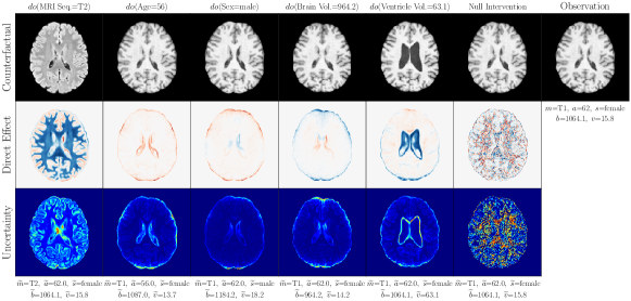
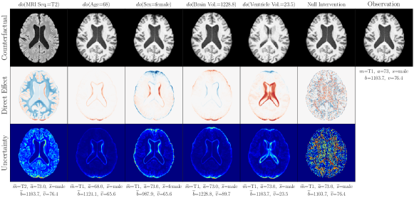
Figure 16: Additional counterfactual results from performing random interventions of each attribute (non-cherrypicked). We observed localized changes in accordance with the interventions performed and the associated assumed causal graph. Crucially, the identity of the original observation is well preserved, indicating that the approximate abduction step is fairly accurate even at high resolutions. As explained in the main text, the direct treatment effect is the difference between the generated counterfactual and the null-intervened (reconstructed) outcome. The per-pixel counterfactual uncertainty maps relate to the uncertainty in the abduction of the $\mathbf{x}$’s exogenous noise, namely $\mathbf{z}_{1:L}$ and $\boldsymbol{\epsilon}$, and were calculated as described in Appendix A.2. using 50 samples from the posterior distribution of the exogenous noise.

‘MRI Seq.’ counterfactuals $do(m)$

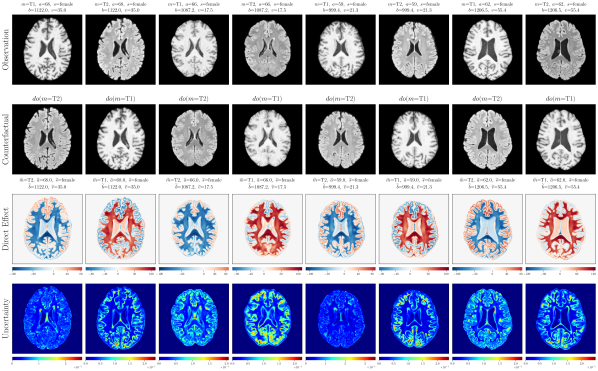
 Post counterfactual training:

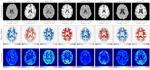
Figure 17: Visualizing brain MRI Seq. ($m$) test set counterfactuals from our Deep SCM using the proposed exogenous prior HVAE for $\mathbf{x}$’s mechanism (non-cherrypicked). Direct treatment effects and per-pixel counterfactual uncertainty maps are also shown. Counterfactuals were obtained from random interventions on T1/T2 ($do(m)$) before (rows 2 to 4) and after counterfactual training (rows 5 to 7). T1 and T2 scans belonging to the same subject are shown side-by-side in pairs.

‘Sex’ counterfactuals $do(s)$

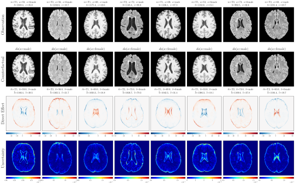
  Post counterfactual training:

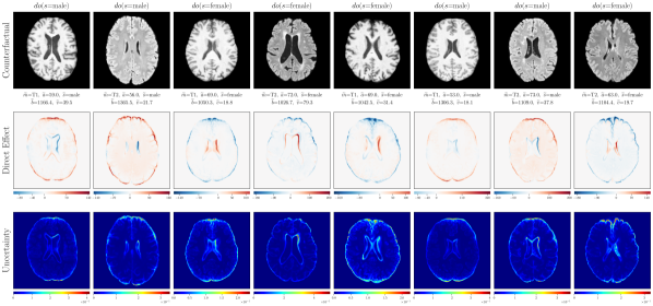
Figure 18: Visualizing brain sex ($s$) test set counterfactuals from our Deep SCM using the proposed exogenous prior HVAE for $\mathbf{x}$’s mechanism (non-cherrypicked). Direct treatment effects and per-pixel counterfactual uncertainty maps are also shown. Counterfactuals were obtained from random interventions on sex ($do(s)$) before (rows 2 to 4) and after counterfactual training (rows 5 to 7).

‘Age’ counterfactuals $do(a)$

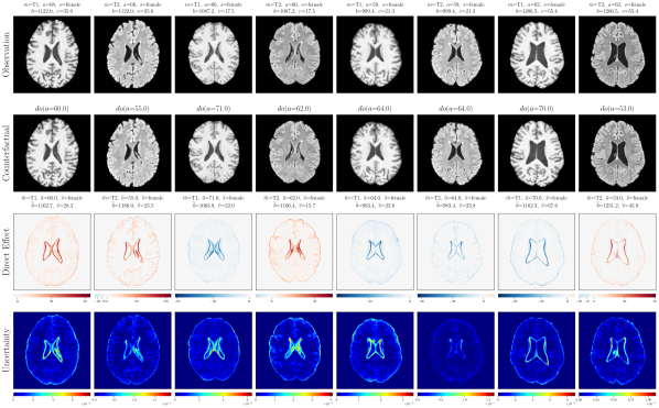
  Post counterfactual training:

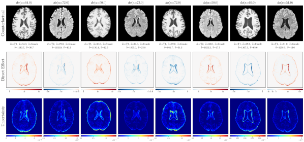
Figure 19: Visualizing brain age ($a$) test set counterfactuals from our Deep SCM using the proposed exogenous prior HVAE for $\mathbf{x}$’s mechanism (non-cherrypicked). Direct treatment effects and per-pixel counterfactual uncertainty maps are also shown. Counterfactuals were obtained from random interventions on age ($do(a)$) before (rows 2 to 4) and after counterfactual training (rows 5 to 7).

‘Brain Volume’ counterfactuals $do(b)$

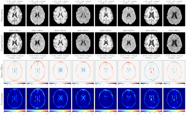
  Post counterfactual training:

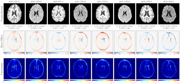
Figure 20: Visualizing brain volume ($b$) test set counterfactuals from our Deep SCM using the proposed exogenous prior HVAE for $\mathbf{x}$’s mechanism (non-cherrypicked). Direct treatment effects and per-pixel counterfactual uncertainty maps are also shown. Counterfactuals were obtained from random interventions on brain vol. ($do(b)$) before (rows 2 to 4) and after counterfactual training (rows 5 to 7).

‘Ventricle Volume’ counterfactuals $do(v)$

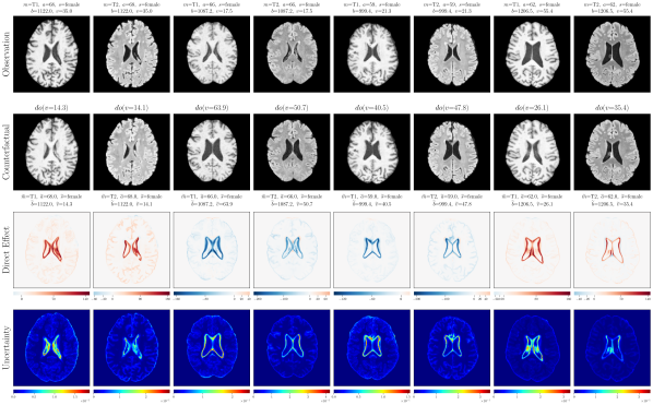
  Post counterfactual training:

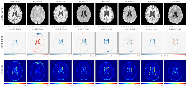
Figure 21: Visualizing ventricle volume ($v$) test set counterfactuals from our Deep SCM using the proposed exogenous prior HVAE for $\mathbf{x}$’s mechanism (non-cherrypicked). Direct treatment effects and per-pixel counterfactual uncertainty maps are also shown. Counterfactuals were obtained from random interventions on ventricle vol. ($do(v)$) before (rows 2 to 4) and after counterfactual training (rows 5 to 7).

Random Samples from full SCM

Figure 22: Random samples from our full structural causal model at different temperatures $t$ per row ($192{\times}192$ resolution, non-cherrypicked). Lower temperature samples ($t<1$) are typically used for more complex datasets. Samples above may sometimes be translated because $\mathbf{x}$’s HVAE mechanism was trained using random cropping data augmentation.

Null-Interventions on full SCM

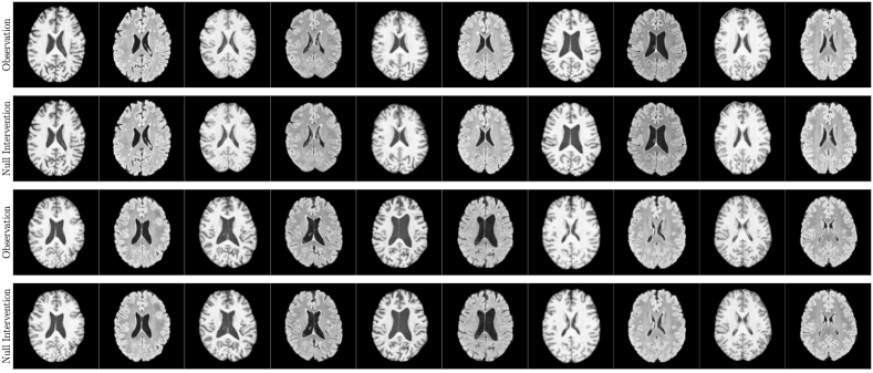
Figure 23: Null intervention results on random test set examples from UK Biobank (non-cherrypicked, using our exogenous prior HVAE as $\mathbf{x}$’s mechanism). Recall that a null intervention is simply the act of intervening on our SCM using values of the parents $\mathbf{pa}_{\mathbf{x}}$ of an observation $\mathbf{x}$. In effect, it is a reconstruction of the input and it measures the composition property.

Appendix E Chest X-ray (MIMIC-CXR)

E.1 Dataset details

We resized all the MIMIC-CXR chest X-ray images to $192{\times}192$ resolution and selected four attributes of interest from the meta-data, namely: sex, race, age and disease. The assumed causal graph is presented in Figure 5. Notably, for disease we only considered Pleural Effusion and filtered the dataset of other diseases. Therefore, our resulting dataset only contains subjects that were either diagnosed as healthy (no finding) or with Pleural Effusion. Finally, we split the dataset into 62,336 subjects for training, 9,968 for validation and 30,535 for testing.

E.2 Experiment setup

Architecture. We used the same exogenous prior HVAE architecture as in the Brain MRI experiments (see Section D.2).

Training details. We trained our HVAEs for $\simeq$210K steps using a batch size of 32 and the AdamW optimizer (Loshchilov & Hutter, 2017). The rest of the training settings are the same as in Section D.2.

E.3 Discrete counterfactuals

For the MIMIC-CXR chest X-ray dataset, we assumed a causal model as shown in Figure 5. In this causal structure, age $a$ was the parent of disease $d$ which represents the existence of Pleural Effusion. Since $d$ is not a continuous variable, normalizing flows could not be directly employed for modelling $d$’s (invertible) mechanism. To solve this, we adopted the discrete mechanisms with the Gumbel-max parametrisation as suggested in Pawlowski et al. (2020), Appendix C. More mathematical details can be found in Maddison & Tarlow (2017); Oberst & Sontag (2019).

The Gumbel-max trick is a method to draw a sample for a discrete distribution, given its probabilities over categories. Suppose we have a discrete random variable $y$ over $K$ categories, with likelihood represented by logits $\bm{\lambda}$:

$$p(y=k)=\frac{e^{\lambda{k}}}{\sum_{n=1}^{K}e^{\lambda{n}}},$$ (36)

Due to a special property of the Gumbel distribution, if we sample $\hat{y}$ by:

$$\hat{y}:={\arg\max}_{k^{\prime}\leq K}(\epsilon_{k^{\prime}}+\lambda_{k^{\prime}}), \epsilon_{k^{\prime}}\sim\text{Gumbel}(0,1),$$ (37)

the resulting $\hat{y}$ has exactly the same distribution as $y$. Furthermore, if we were to observe $y=k$, then we can infer the values of $\bm{\epsilon}$ by sampling from the exact posterior as follows:

$$\hat{\epsilon}_{k} =G_{k}+\log\sum_{l=1}^{K}e^{\lambda_{l}}-\lambda_{k}, G_{k}\sim\text{Gumbel}(0,1),$$ (38)

$$\hat{\epsilon}_{i} =-\log(e^{-G_{i}-\lambda_{i}}+e^{-\hat{\epsilon}}_{k}-\lambda_{k})-\lambda_{i}, G_{i}\sim\text{Gumbel}(0,1),\ i\neq k.$$ (39)

We can then formulate the (approximately) invertible mechanism for a discrete attribute $y$ with parents $\mathbf{pa}_{{y}}$ by making $\bm{\lambda}$ a function of $\mathbf{pa_{{y}}}$ via a neural network $g_{y}$. Thus, the forward mechanism $f_{y}$ to generate $y$ given its parents $\mathbf{pa}_{y}$ consists of first computing the logits $\bm{\lambda}$, then sampling via Eq. 37:

$$y:=f_{y}(\bm{\epsilon},\mathbf{pa}_{y})={\arg\max}_{k^{\prime}\leq K}(\epsilon_{k^{\prime}}+\lambda_{k^{\prime}}), \bm{\lambda}=g_{y}(\mathbf{pa}_{y}), \epsilon_{k^{\prime}}\sim\text{Gumbel}(0,1).$$ (40)

Moreover, when we perform an upstream intervention on $\widetilde{\mathbf{pa}}_{y}$ yielding: $\bm{\widetilde{\lambda}}=g(\mathbf{\widetilde{pa}}_{y})$, we can (non-deterministically) compute the counterfactual outcome $\widetilde{y}$ by first inferring $\bm{\hat{\epsilon}}$ from the exact posterior via Eq. 38 using the original (observational) logits $\bm{\lambda}$, and then computing $\widetilde{y}$ via Eq. 37 using $\bm{\widetilde{\lambda}}$ and the inferred $\bm{\hat{\epsilon}}$.

E.4 Extra results

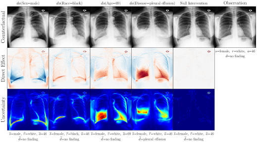
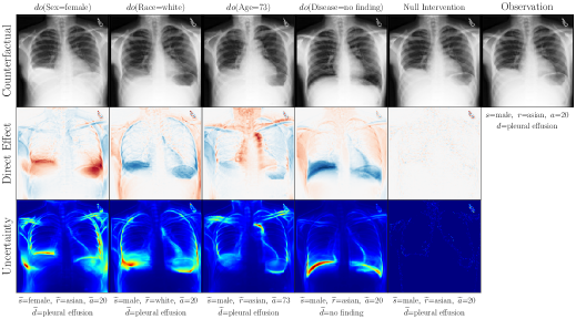
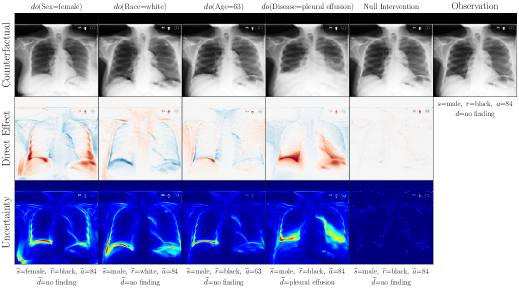
Figure 24: Additional counterfactuals from random interventions of each attribute on the chest X-ray test set. We observed localized changes in accordance with the interventions performed and the associated assumed causal graph. Crucially, the identity of the original observation is well preserved, indicating that the approximate abduction step is fairly accurate even at high resolutions. The direct causal effect is the difference between the generated counterfactual and the null-intervened (reconstructed) outcome. The per-pixel counterfactual uncertainty maps relate to the uncertainty in the abduction of the $\mathbf{x}$’s exogenous noise and were calculated as described in Appendix A.2 using 32 samples from the posterior distribution.

‘Sex’ counterfactuals $do(s)$

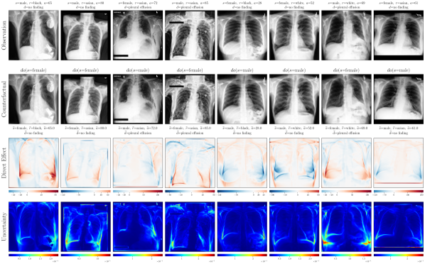
  Post counterfactual training:

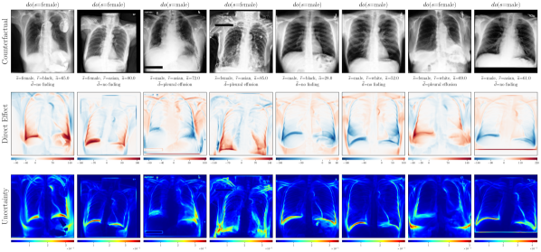
Figure 25: Visualizing chest sex ($s$) test set counterfactuals from our Deep SCM using the proposed exogenous prior HVAE for $\mathbf{x}$’s mechanism (non-cherrypicked). Direct treatment effects and per-pixel counterfactual uncertainty maps are also shown. Counterfactuals were obtained from random interventions on sex ($do(s)$) before (rows 2 to 4) and after counterfactual training (rows 5 to 7).

‘Race’ counterfactuals $do(r)$

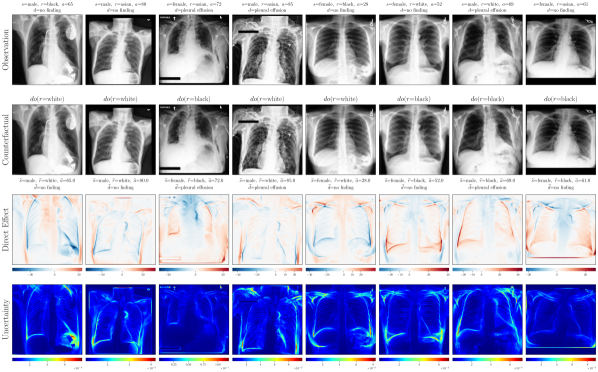
  Post counterfactual training:

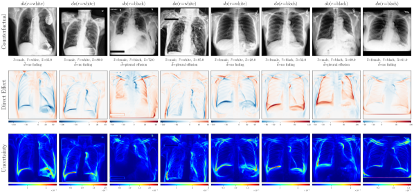
Figure 26: Visualizing chest race ($r$) test set counterfactuals from our Deep SCM using the proposed exogenous prior HVAE for $\mathbf{x}$’s mechanism (non-cherrypicked). Direct treatment effects and per-pixel counterfactual uncertainty maps are also shown. Counterfactuals were obtained from random interventions on race ($do(r)$) before (rows 2 to 4) and after counterfactual training (rows 5 to 7).

‘Age’ counterfactuals $do(a)$

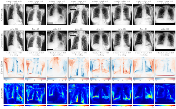
  Post counterfactual training:

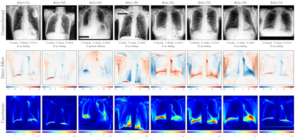
Figure 27: Visualizing chest age ($age$) test set counterfactuals from our Deep SCM using the proposed exogenous prior HVAE for $\mathbf{x}$’s mechanism (non-cherrypicked). Direct treatment effects and per-pixel counterfactual uncertainty maps are also shown. Counterfactuals were obtained from random interventions on age ($do(age)$) before (rows 2 to 4) and after counterfactual training (rows 5 to 7).

‘Disease’ counterfactuals $do(d)$

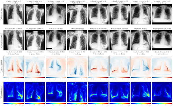
  Post counterfactual training:

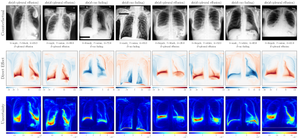
Figure 28: Visualizing chest disease ($d$) test set counterfactuals from our Deep SCM using the proposed exogenous prior HVAE for $\mathbf{x}$’s mechanism (non-cherrypicked). Direct treatment effects and per-pixel counterfactual uncertainty maps are also shown. Counterfactuals were obtained from random interventions on disease ($do(d)$) before (rows 2 to 4) and after counterfactual training (rows 5 to 7).

Null-Interventions on full SCM

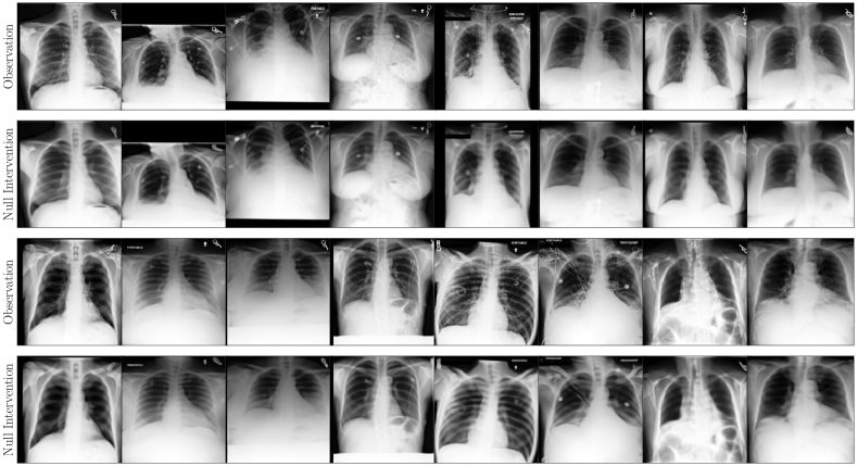
Figure 29: Null intervention results on random test set examples from MIMIC-CXR (non-cherrypicked, using our exogenous prior HVAE as $\mathbf{x}$’s mechanism). Recall that a null intervention is simply the act of intervening on our SCM using values of the parents $\mathbf{pa}_{\mathbf{x}}$ of an observation $\mathbf{x}$. In effect, it is a reconstruction of the input and it measures the composition property.

Appendix F Anticausal Predictors $q_{\psi}(k\mid\mathbf{pa}_{k})$

⬇

class MLP(nn.Module):

def __init__(self, num_inputs=1, width=32, num_outputs=1):

super().__init__()

activation = nn.LeakyReLU()

self.mlp = nn.Sequential(

nn.Linear(num_inputs, width, bias=False),

nn.BatchNorm1d(width),

activation,

nn.Linear(width, width, bias=False),

nn.BatchNorm1d(width),

activation,

nn.Linear(width, num_outputs),

)

\pardef forward(self, x):

return self.mlp(x)

⬇

class CNN(nn.Module):

def __init__(self, in_shape, width=16, num_outputs=1, context_dim=0):

super().__init__()

in_channels = in_shape[0]

res = in_shape[1]

s = 2 if res > 64 else 1

activation = nn.LeakyReLU()

self.cnn = nn.Sequential(

nn.Conv2d(in_channels, width, 7, s, 3, bias=False),

nn.BatchNorm2d(width),

activation,

(nn.MaxPool2d(2, 2) if res > 32 else nn.Identity()),

nn.Conv2d(width, 2*width, 3, 2, 1, bias=False),

nn.BatchNorm2d(2*width),

activation,

nn.Conv2d(2*width, 2*width, 3, 1, 1, bias=False),

nn.BatchNorm2d(2*width),

activation,

nn.Conv2d(2*width, 4*width, 3, 2, 1, bias=False),

nn.BatchNorm2d(4*width),

activation,

nn.Conv2d(4*width, 4*width, 3, 1, 1, bias=False),

nn.BatchNorm2d(4*width),

activation,

nn.Conv2d(4*width, 8*width, 3, 2, 1, bias=False),

nn.BatchNorm2d(8*width),

activation

)

self.fc = nn.Sequential(

nn.Linear(8*width + context_dim, 8*width, bias=False),

nn.BatchNorm1d(8*width),

activation,

nn.Linear(8*width, num_outputs)

)

\pardef forward(self, x, y=None):

x = self.cnn(x)

x = x.mean(dim=(-2, -1)) # avg pool

if y is not None:

x = torch.cat([x, y], dim=-1)

return self.fc(x)

Architecture.

The parent predictors (classifiers/regressors) shown in the PyTorch code above were used for both Morpho-MNIST and the Brain MRI dataset and were trained using Pyro. For MIMIC-CXR dataset, we adopted the standard ResNet-18 (He et al., 2016) architecture pre-defined in Torchvision (Paszke et al., 2019) for the parent predictors. These predictors play two roles in our approach: (i) to serve as pseudo-oracles in evaluating the effectiveness of generated counterfactuals; (ii) to provide guidance during our proposed counterfactual training technique. For both purposes, our parent predictors are trained on observational data and in the anticausal direction with respect to each variable in the assumed SCM. That is, each variable is predicted from its children. When a variable in the SCM is not a direct parent of the image $\mathbf{x}$, we use the MLP architecture for its predictor, otherwise, we use the CNN. As a side note, missing values for some of the parents in our observed data can restrict the applicability of SCMs. In order to handle missing values, we can use variational predictors to infer parent attributes in the anticausal direction. That is, when a certain parent is not present in an observed datum, we can infer it given its observed children (imputation). The inferred parent may then be used downstream as if it was observed to, e.g. compute approximate counterfactuals.

Table 6: Attribute predictor performance on UK Biobank observational data.

Sex $(s)$	MRI $(m)$	Age $(a)$	Brain Vol. $(b)$	Ventricle Vol. $(v)$
ROCAUC $\uparrow$	ROCAUC $\uparrow$	MAE (years) $\downarrow$	MAE (ml) $\downarrow$	MAE (ml) $\downarrow$
0.9764 $\pm$ 2e-3	1.0	4.847 $\pm$ 7e-4	26.77 $\pm$ 0.39	1.958 $\pm$ 3e-2

Table 7: Attribute predictor performance on MIMIC-CXR observational data.

Sex $(s)$	Race $(m)$	Age $(a)$	Disease $(d)$
ROCAUC $\uparrow$	ROCAUC $\uparrow$	MAE (years) $\downarrow$	ROCAUC $\uparrow$
0.9950	0.7496	6.219	0.9419

Predictor Training Details.

For each dataset, we train the predictors for all parents simultaneously until convergence, where the total loss is simply the sum of all the individual predictor losses. We use a batch size of 32, and use the AdamW optimizer with a learning rate of 1e-4 and weight decay of 0.1 for UK Biobank, 0.01 for Morpho-MNIST and 0.05 for MIMIC-CXR. The final artefacts are an exponential moving average of the predictor’s parameters with a rate of 0.999, which we use at inference time. For data augmentation, we random crop with an all-border zero-padding of 4 for Morpho-MNIST 9 for UK Biobank and MIMIC-CXR. We further perform random horizontal flips with probability 0.5 for UK Biobank. Pixel intensities were rescaled to $[-1,1]$ for all datasets.

Counterfactual Training Details.

As described in the main text, once all the mechanisms in the SCM of interest have been trained, they are combined into one PyTorch module which we use for counterfactual training/inference. For the Brain MRI and Chext X-ray datasets, we found it most effective to freeze all other mechanisms (including parent predictors) in the SCM during constrained counterfactual fine-tuning of $\mathbf{x}$’s HVAE mechanism – since we care mostly about the quality/faithfulness of $\widetilde{\mathbf{x}}$ counterfactuals. For counterfactual fine-tuning, we start with the exponential moving average of the pre-trained HVAE parameters, and use the AdamW optimizer with a learning rate 10${\times}$ smaller than what was used to originally train the HVAE mechanism, 1e-4. All else remain the same as the original HVAE training setup except for the batch size which was decreased to 24 due to GPU memory constraints. To train the Lagrange multiplier parameter $\lambda$, we used a separate AdamW optimizer with a learning rate of 0.1, and initialised $\lambda$ at 10. We optimize the Lagrangian in Eq. (26) by performing stochastic gradient descent on the HVAE’s parameters and ascent on the Lagrange multiplier. We observed that training for around 10K iterations was sufficient to achieve the desired effect on the brain MRI data, and training for 6.5K iterations led to desirable performance on the chest X-ray data. Note that the efficacy of this strategy is entirely dependent on the quality of the initial parent predictors used for counterfactual training. Moreover, in order to help identify whether the model learned shortcuts in producing effective interventions, we ensured that we used separately trained anticausal predictors for counterfactual training and for the subsequent counterfactual effectiveness evaluation. As is the case with all types of classifier-based guidance, it is important to keep the possibility of shortcut learning in mind when using counterfactual training, and to take precautions to mitigate it. Using more robust classifiers with smoother loss surfaces (e.g. Bayesian predictors, adversarial training techniques etc) may prove particularly helpful.

References

- Alfaro-Almagro et al. (2018) Alfaro-Almagro, F., Jenkinson, M., Bangerter, N. K., Andersson, J. L., Griffanti, L., Douaud, G., Sotiropoulos, S. N., Jbabdi, S., Hernandez-Fernandez, M., Vallee, E., et al. Image processing and quality control for the first 10,000 brain imaging datasets from uk biobank. Neuroimage, 166:400–424, 2018.
- Balashankar et al. (2021) Balashankar, A., Wang, X., Packer, B., Thain, N., Chi, E., and Beutel, A. Can we improve model robustness through secondary attribute counterfactuals? In Proceedings of the 2021 Conference on Empirical Methods in Natural Language Processing, pp. 4701–4712, 2021.
- Barber & Agakov (2004) Barber, D. and Agakov, F. The im algorithm: a variational approach to information maximization. Advances in neural information processing systems, 16(320):201, 2004.
- Bareinboim et al. (2022) Bareinboim, E., Correa, J. D., Ibeling, D., and Icard, T. On Pearl’s Hierarchy and the Foundations of Causal Inference, pp. 507–556. Association for Computing Machinery, New York, NY, USA, 1 edition, 2022. ISBN 9781450395861. URL https://doi.org/10.1145/3501714.3501743.
- Bengio et al. (2013) Bengio, Y., Courville, A., and Vincent, P. Representation learning: a review and new perspectives. IEEE transactions on pattern analysis and machine intelligence, 35(8):1798—1828, August 2013. ISSN 0162-8828. doi: 10.1109/tpami.2013.50.
- Bernhardt et al. (2022) Bernhardt, M., Jones, C., and Glocker, B. Potential sources of dataset bias complicate investigation of underdiagnosis by machine learning algorithms. Nature Medicine, 28(6):1157–1158, 2022.
- Bingham et al. (2019) Bingham, E., Chen, J. P., Jankowiak, M., Obermeyer, F., Pradhan, N., Karaletsos, T., Singh, R., Szerlip, P., Horsfall, P., and Goodman, N. D. Pyro: Deep universal probabilistic programming. The Journal of Machine Learning Research, 20(1):973–978, 2019.
- Brooks et al. (2022) Brooks, T., Holynski, A., and Efros, A. A. Instructpix2pix: Learning to follow image editing instructions. arXiv preprint arXiv:2211.09800, 2022.
- Burda et al. (2015) Burda, Y., Grosse, R., and Salakhutdinov, R. Importance weighted autoencoders. arXiv preprint arXiv:1509.00519, 2015.
- Castro et al. (2019) Castro, D. C., Tan, J., Kainz, B., Konukoglu, E., and Glocker, B. Morpho-mnist: quantitative assessment and diagnostics for representation learning. Journal of Machine Learning Research, 20(178):1–29, 2019.
- Castro et al. (2020) Castro, D. C., Walker, I., and Glocker, B. Causality matters in medical imaging. Nature Communications, 11(1):1–10, 2020.
- Chen et al. (2018) Chen, R. T., Li, X., Grosse, R. B., and Duvenaud, D. K. Isolating sources of disentanglement in variational autoencoders. Advances in neural information processing systems, 31, 2018.
- Chen et al. (2016) Chen, X., Duan, Y., Houthooft, R., Schulman, J., Sutskever, I., and Abbeel, P. Infogan: Interpretable representation learning by information maximizing generative adversarial nets. Advances in neural information processing systems, 29, 2016.
- Child (2020) Child, R. Very deep vaes generalize autoregressive models and can outperform them on images. In International Conference on Learning Representations, 2020.
- D’Amour et al. (2022) D’Amour, A., Heller, K., Moldovan, D., Adlam, B., Alipanahi, B., Beutel, A., Chen, C., Deaton, J., Eisenstein, J., Hoffman, M. D., et al. Underspecification presents challenges for credibility in modern machine learning. The Journal of Machine Learning Research, 23(1):10237–10297, 2022.
- Dhariwal & Nichol (2021) Dhariwal, P. and Nichol, A. Diffusion models beat gans on image synthesis. Advances in Neural Information Processing Systems, 34:8780–8794, 2021.
- Galles & Pearl (1998) Galles, D. and Pearl, J. An axiomatic characterization of causal counterfactuals. Foundations of Science, 3:151–182, 1998. ISSN 1572-8471. doi: 10.1023/A:1009602825894.
- Geffner et al. (2022) Geffner, T., Antoran, J., Foster, A., Gong, W., Ma, C., Kiciman, E., Sharma, A., Lamb, A., Kukla, M., Pawlowski, N., et al. Deep end-to-end causal inference. arXiv preprint arXiv:2202.02195, 2022.
- Glocker et al. (2023) Glocker, B., Jones, C., Bernhardt, M., and Winzeck, S. Algorithmic encoding of protected characteristics in chest x-ray disease detection models. Ebiomedicine, 89, 2023.
- Goodfellow et al. (2020) Goodfellow, I., Pouget-Abadie, J., Mirza, M., Xu, B., Warde-Farley, D., Ozair, S., Courville, A., and Bengio, Y. Generative adversarial networks. Communications of the ACM, 63(11):139–144, 2020.
- Halpern (1998) Halpern, J. Y. Axiomatizing causal reasoning. In Proceedings of the Fourteenth Conference on Uncertainty in Artificial Intelligence, UAI’98, pp. 202–210, San Francisco, CA, USA, 1998. Morgan Kaufmann Publishers Inc. ISBN 155860555X.
- He et al. (2016) He, K., Zhang, X., Ren, S., and Sun, J. Deep residual learning for image recognition. In Proceedings of the IEEE conference on computer vision and pattern recognition, pp. 770–778, 2016.
- Higgins et al. (2017) Higgins, I., Matthey, L., Pal, A., Burgess, C., Glorot, X., Botvinick, M., Mohamed, S., and Lerchner, A. beta-vae: Learning basic visual concepts with a constrained variational framework. In 5th International Conference on Learning Representations, ICLR 2017, 2017.
- Hinton et al. (1995) Hinton, G. E., Dayan, P., Frey, B. J., and Neal, R. M. The” wake-sleep” algorithm for unsupervised neural networks. Science, 268(5214):1158–1161, 1995.
- Ho & Salimans (2022) Ho, J. and Salimans, T. Classifier-free diffusion guidance. arXiv preprint arXiv:2207.12598, 2022.
- Ho et al. (2020) Ho, J., Jain, A., and Abbeel, P. Denoising diffusion probabilistic models. Advances in Neural Information Processing Systems, 33:6840–6851, 2020.
- Hyvarinen et al. (2019) Hyvarinen, A., Sasaki, H., and Turner, R. Nonlinear ica using auxiliary variables and generalized contrastive learning. In The 22nd International Conference on Artificial Intelligence and Statistics, pp. 859–868. PMLR, 2019.
- Imai et al. (2010) Imai, K., Keele, L., and Yamamoto, T. Identification, inference and sensitivity analysis for causal mediation effects. Statistical science, 25(1):51–71, 2010.
- Isola et al. (2017) Isola, P., Zhu, J.-Y., Zhou, T., and Efros, A. A. Image-to-image translation with conditional adversarial networks. In 2017 IEEE Conference on Computer Vision and Pattern Recognition (CVPR), pp. 5967–5976, 2017. doi: 10.1109/CVPR.2017.632.
- Johnson et al. (2019) Johnson, A. E., Pollard, T. J., Berkowitz, S. J., Greenbaum, N. R., Lungren, M. P., Deng, C.-y., Mark, R. G., and Horng, S. Mimic-cxr, a de-identified publicly available database of chest radiographs with free-text reports. Scientific data, 6(1):1–8, 2019.
- Karras et al. (2019) Karras, T., Laine, S., and Aila, T. A style-based generator architecture for generative adversarial networks. In Proceedings of the IEEE/CVF conference on computer vision and pattern recognition, pp. 4401–4410, 2019.
- Kaushik et al. (2020) Kaushik, D., Hovy, E., and Lipton, Z. Learning the difference that makes a difference with counterfactually-augmented data. In International Conference on Learning Representations, 2020. URL https://openreview.net/forum?id=Sklgs0NFvr.
- Ke et al. (2019) Ke, N. R., Bilaniuk, O., Goyal, A., Bauer, S., Larochelle, H., Schölkopf, B., Mozer, M. C., Pal, C., and Bengio, Y. Learning neural causal models from unknown interventions. arXiv preprint arXiv:1910.01075, 2019.
- Khemakhem et al. (2020) Khemakhem, I., Kingma, D., Monti, R., and Hyvarinen, A. Variational autoencoders and nonlinear ica: A unifying framework. In International Conference on Artificial Intelligence and Statistics, pp. 2207–2217. PMLR, 2020.
- Kim & Mnih (2018) Kim, H. and Mnih, A. Disentangling by factorising. In Proceedings of the 35th International Conference on Machine Learning, volume 80 of Proceedings of Machine Learning Research, pp. 2649–2658. PMLR, 10–15 Jul 2018.
- Kingma et al. (2021) Kingma, D., Salimans, T., Poole, B., and Ho, J. Variational diffusion models. Advances in neural information processing systems, 34:21696–21707, 2021.
- Kingma & Welling (2013) Kingma, D. P. and Welling, M. Auto-encoding variational bayes. arXiv preprint arXiv:1312.6114, 2013.
- Kingma et al. (2016) Kingma, D. P., Salimans, T., Jozefowicz, R., Chen, X., Sutskever, I., and Welling, M. Improved variational inference with inverse autoregressive flow. Advances in neural information processing systems, 29, 2016.
- Kocaoglu et al. (2017) Kocaoglu, M., Snyder, C., Dimakis, A. G., and Vishwanath, S. Causalgan: Learning causal implicit generative models with adversarial training. arXiv preprint arXiv:1709.02023, 2017.
- Kocaoglu et al. (2018) Kocaoglu, M., Snyder, C., Dimakis, A. G., and Vishwanath, S. CausalGAN: Learning causal implicit generative models with adversarial training. In International Conference on Learning Representations, 2018. URL https://openreview.net/forum?id=BJE-4xW0W.
- Kusner et al. (2017) Kusner, M. J., Loftus, J., Russell, C., and Silva, R. Counterfactual fairness. Advances in neural information processing systems, 30, 2017.
- Liu et al. (2017) Liu, M.-Y., Breuel, T., and Kautz, J. Unsupervised image-to-image translation networks. Advances in neural information processing systems, 30, 2017.
- Locatello et al. (2019) Locatello, F., Bauer, S., Lucic, M., Raetsch, G., Gelly, S., Schölkopf, B., and Bachem, O. Challenging common assumptions in the unsupervised learning of disentangled representations. In international conference on machine learning, pp. 4114–4124. PMLR, 2019.
- Loshchilov & Hutter (2017) Loshchilov, I. and Hutter, F. Decoupled weight decay regularization. arXiv preprint arXiv:1711.05101, 2017.
- Louizos et al. (2017) Louizos, C., Shalit, U., Mooij, J. M., Sontag, D., Zemel, R., and Welling, M. Causal effect inference with deep latent-variable models. Advances in neural information processing systems, 30, 2017.
- Maaløe et al. (2019) Maaløe, L., Fraccaro, M., Liévin, V., and Winther, O. Biva: A very deep hierarchy of latent variables for generative modeling. Advances in neural information processing systems, 32, 2019.
- Maddison & Tarlow (2017) Maddison, C. and Tarlow, D. Gumbel machinery. https://cmaddis.github.io/gumbel-machinery, 2017.
- Mirza & Osindero (2014) Mirza, M. and Osindero, S. Conditional generative adversarial nets. arXiv preprint arXiv:1411.1784, 2014.
- Monteiro et al. (2023) Monteiro, M., Ribeiro, F. D. S., Pawlowski, N., Castro, D. C., and Glocker, B. Measuring axiomatic soundness of counterfactual image models. In The Eleventh International Conference on Learning Representations, 2023. URL https://openreview.net/forum?id=lZOUQQvwI3q.
- Mothilal et al. (2020) Mothilal, R. K., Sharma, A., and Tan, C. Explaining machine learning classifiers through diverse counterfactual explanations. In Proceedings of the 2020 conference on fairness, accountability, and transparency, pp. 607–617, 2020.
- Nielsen et al. (2020) Nielsen, D., Jaini, P., Hoogeboom, E., Winther, O., and Welling, M. Survae flows: Surjections to bridge the gap between vaes and flows. Advances in Neural Information Processing Systems, 33:12685–12696, 2020.
- Oberst & Sontag (2019) Oberst, M. and Sontag, D. Counterfactual off-policy evaluation with gumbel-max structural causal models. In International Conference on Machine Learning, pp. 4881–4890. PMLR, 2019.
- Paszke et al. (2019) Paszke, A., Gross, S., Massa, F., Lerer, A., Bradbury, J., Chanan, G., Killeen, T., Lin, Z., Gimelshein, N., Antiga, L., et al. Pytorch: An imperative style, high-performance deep learning library. Advances in neural information processing systems, 32, 2019.
- Pawlowski et al. (2020) Pawlowski, N., Coelho de Castro, D., and Glocker, B. Deep structural causal models for tractable counterfactual inference. Advances in Neural Information Processing Systems, 33:857–869, 2020.
- Pearl (2001) Pearl, J. Direct and indirect effects. In Proceedings of the Seventeenth Conference on Uncertainty in Artificial Intelligence, UAI’01, pp. 411–420, San Francisco, CA, USA, 2001. Morgan Kaufmann Publishers Inc. ISBN 1558608001.
- Pearl (2009) Pearl, J. Causality. Cambridge university press, 2009.
- Peters et al. (2017) Peters, J., Janzing, D., and Schölkopf, B. Elements of causal inference: foundations and learning algorithms. The MIT Press, 2017.
- Platt & Barr (1987) Platt, J. and Barr, A. Constrained differential optimization. In Neural Information Processing Systems, 1987.
- Preechakul et al. (2022) Preechakul, K., Chatthee, N., Wizadwongsa, S., and Suwajanakorn, S. Diffusion autoencoders: Toward a meaningful and decodable representation. In Proceedings of the IEEE/CVF Conference on Computer Vision and Pattern Recognition, pp. 10619–10629, 2022.
- Reizinger et al. (2022) Reizinger, P., Gresele, L., Brady, J., von Kügelgen, J., Zietlow, D., Schölkopf, B., Martius, G., Brendel, W., and Besserve, M. Embrace the gap: Vaes perform independent mechanism analysis. In Koyejo, S., Mohamed, S., Agarwal, A., Belgrave, D., Cho, K., and Oh, A. (eds.), Advances in Neural Information Processing Systems, volume 35, pp. 12040–12057. Curran Associates, Inc., 2022.
- Rezende & Mohamed (2015) Rezende, D. and Mohamed, S. Variational inference with normalizing flows. In International conference on machine learning, pp. 1530–1538. PMLR, 2015.
- Rezende et al. (2014) Rezende, D. J., Mohamed, S., and Wierstra, D. Stochastic backpropagation and approximate inference in deep generative models. In International conference on machine learning, pp. 1278–1286. PMLR, 2014.
- Robins & Greenland (1992) Robins, J. M. and Greenland, S. Identifiability and exchangeability for direct and indirect effects. Epidemiology, pp. 143–155, 1992.
- Saharia et al. (2022) Saharia, C., Chan, W., Chang, H., Lee, C., Ho, J., Salimans, T., Fleet, D., and Norouzi, M. Palette: Image-to-image diffusion models. In ACM SIGGRAPH 2022 Conference Proceedings, pp. 1–10, 2022.
- Sanchez & Tsaftaris (2021) Sanchez, P. and Tsaftaris, S. A. Diffusion causal models for counterfactual estimation. In First Conference on Causal Learning and Reasoning, 2021.
- Sanchez et al. (2022a) Sanchez, P., Kascenas, A., Liu, X., O’Neil, A. Q., and Tsaftaris, S. A. What is healthy? generative counterfactual diffusion for lesion localization. In Deep Generative Models: Second MICCAI Workshop, DGM4MICCAI 2022, Held in Conjunction with MICCAI 2022, Singapore, September 22, 2022, Proceedings, pp. 34–44. Springer, 2022a.
- Sanchez et al. (2022b) Sanchez, P., Liu, X., O’Neil, A. Q., and Tsaftaris, S. A. Diffusion models for causal discovery via topological ordering. arXiv preprint arXiv:2210.06201, 2022b.
- Schölkopf (2022) Schölkopf, B. Causality for Machine Learning, pp. 765–804. Association for Computing Machinery, New York, NY, USA, 1 edition, 2022. ISBN 9781450395861. URL https://doi.org/10.1145/3501714.3501755.
- Schölkopf et al. (2021) Schölkopf, B., Locatello, F., Bauer, S., Ke, N. R., Kalchbrenner, N., Goyal, A., and Bengio, Y. Toward causal representation learning. Proceedings of the IEEE, 109(5):612–634, 2021.
- Schut et al. (2021) Schut, L., Key, O., Mc Grath, R., Costabello, L., Sacaleanu, B., Gal, Y., et al. Generating interpretable counterfactual explanations by implicit minimisation of epistemic and aleatoric uncertainties. In International Conference on Artificial Intelligence and Statistics, pp. 1756–1764. PMLR, 2021.
- Seyyed-Kalantari et al. (2020) Seyyed-Kalantari, L., Liu, G., McDermott, M., Chen, I. Y., and Ghassemi, M. Chexclusion: Fairness gaps in deep chest x-ray classifiers. In BIOCOMPUTING 2021: proceedings of the Pacific symposium, pp. 232–243. World Scientific, 2020.
- Shu & Ermon (2022) Shu, R. and Ermon, S. Bit prioritization in variational autoencoders via progressive coding. In International Conference on Machine Learning, pp. 20141–20155. PMLR, 2022.
- Simon (1954) Simon, H. A. Spurious correlation: A causal interpretation. Journal of the American statistical Association, 49(267):467–479, 1954.
- Sohl-Dickstein et al. (2015) Sohl-Dickstein, J., Weiss, E., Maheswaranathan, N., and Ganguli, S. Deep unsupervised learning using nonequilibrium thermodynamics. In International Conference on Machine Learning, pp. 2256–2265. PMLR, 2015.
- Sohn et al. (2015) Sohn, K., Lee, H., and Yan, X. Learning structured output representation using deep conditional generative models. Advances in neural information processing systems, 28, 2015.
- Sønderby et al. (2016) Sønderby, C. K., Raiko, T., Maaløe, L., Sønderby, S. K., and Winther, O. Ladder variational autoencoders. Advances in neural information processing systems, 29, 2016.
- Song et al. (2021a) Song, J., Meng, C., and Ermon, S. Denoising diffusion implicit models. In International Conference on Learning Representations, 2021a. URL https://openreview.net/forum?id=St1giarCHLP.
- Song et al. (2021b) Song, Y., Sohl-Dickstein, J., Kingma, D. P., Kumar, A., Ermon, S., and Poole, B. Score-based generative modeling through stochastic differential equations. In International Conference on Learning Representations, 2021b. URL https://openreview.net/forum?id=PxTIG12RRHS.
- Su et al. (2022) Su, X., Song, J., Meng, C., and Ermon, S. Dual diffusion implicit bridges for image-to-image translation. arXiv preprint arXiv:2203.08382, 2022.
- Sudlow et al. (2015) Sudlow, C., Gallacher, J., Allen, N., Beral, V., Burton, P., Danesh, J., Downey, P., Elliott, P., Green, J., Landray, M., et al. Uk biobank: an open access resource for identifying the causes of a wide range of complex diseases of middle and old age. PLoS medicine, 12(3):e1001779, 2015.
- Tabak & Vanden-Eijnden (2010) Tabak, E. G. and Vanden-Eijnden, E. Density estimation by dual ascent of the log-likelihood. Communications in Mathematical Sciences, 8(1):217–233, 2010.
- Tran & Blei (2017) Tran, D. and Blei, D. M. Implicit causal models for genome-wide association studies. arXiv preprint arXiv:1710.10742, 2017.
- Trippe & Turner (2018) Trippe, B. L. and Turner, R. E. Conditional density estimation with bayesian normalising flows. arXiv preprint arXiv:1802.04908, 2018.
- Vahdat & Kautz (2020) Vahdat, A. and Kautz, J. Nvae: A deep hierarchical variational autoencoder. Advances in Neural Information Processing Systems, 33:19667–19679, 2020.
- Van Looveren & Klaise (2021) Van Looveren, A. and Klaise, J. Interpretable counterfactual explanations guided by prototypes. In Machine Learning and Knowledge Discovery in Databases. Research Track: European Conference, ECML PKDD 2021, Bilbao, Spain, September 13–17, 2021, Proceedings, Part II 21, pp. 650–665. Springer, 2021.
- Wachter et al. (2017) Wachter, S., Mittelstadt, B., and Russell, C. Counterfactual explanations without opening the black box: Automated decisions and the gdpr. Harv. JL & Tech., 31:841, 2017.
- Xia et al. (2021) Xia, K., Lee, K.-Z., Bengio, Y., and Bareinboim, E. The causal-neural connection: Expressiveness, learnability, and inference. Advances in Neural Information Processing Systems, 34:10823–10836, 2021.
- Xia et al. (2023) Xia, K. M., Pan, Y., and Bareinboim, E. Neural causal models for counterfactual identification and estimation. In The Eleventh International Conference on Learning Representations, 2023. URL https://openreview.net/forum?id=vouQcZS8KfW.
- Xia et al. (2022a) Xia, T., Sanchez, P., Qin, C., and Tsaftaris, S. A. Adversarial counterfactual augmentation: Application in alzheimer’s disease classification. Frontiers in Radiology, 2022a.
- Xia et al. (2022b) Xia, W., Zhang, Y., Yang, Y., Xue, J.-H., Zhou, B., and Yang, M.-H. Gan inversion: A survey. IEEE Transactions on Pattern Analysis and Machine Intelligence, 2022b.
- Yang et al. (2021) Yang, M., Liu, F., Chen, Z., Shen, X., Hao, J., and Wang, J. Causalvae: Disentangled representation learning via neural structural causal models. In Proceedings of the IEEE/CVF Conference on Computer Vision and Pattern Recognition, pp. 9593–9602, 2021.
- Zečević et al. (2021) Zečević, M., Dhami, D. S., Veličković, P., and Kersting, K. Relating graph neural networks to structural causal models. arXiv preprint arXiv:2109.04173, 2021.
- Zhang & Bareinboim (2018) Zhang, J. and Bareinboim, E. Fairness in decision-making—the causal explanation formula. In Proceedings of the AAAI Conference on Artificial Intelligence, volume 32, 2018.