On the reconstruction of bandlimited signals from random samples quantized via noise-shaping

Abstract.

Noise-shaping quantization techniques are widely used for converting bandlimited signals from the analog to the digital domain. They work by “shaping” the quantization noise so that it falls close to the reconstruction operator’s null space. We investigate the compatibility of two such schemes, specifically $\Sigma\Delta$ quantization and distributed noise-shaping quantization, with random samples of bandlimited functions. Let $f$ be a real-valued $\pi$-bandlimited function. Suppose $R>1$ is a real number and assume that $\{x_{i}\}_{i=1}^{m}$ is a sequence of i.i.d random variables uniformly distributed on $[-\tilde{R},\tilde{R}]$, where $\tilde{R}>R$ is appropriately chosen. We show that by using a noise-shaping quantizer to quantize the values of $f$ at $\{x_{i}\}_{i=1}^{m}$, a function $f^{\sharp}$ can be reconstructed from these quantized values such that $\|f-f^{\sharp}\|_{L^{2}[-R,R]}$ decays with high probability as $m$ and $\tilde{R}$ increase. We emphasize that the sample points $\{x_{i}\}_{i=1}^{m}$ are completely random, i.e., they have no predefined structure, which makes our findings the first of their kind.

1. Introduction

In signal processing, one of the primary goals is to obtain a digital representation of a function in a signal space suitable for storage, transmission and recovery. This goal is usually attained through two steps, sampling and quantization. In the first step of sampling, we sample the function at appropriate data points, referred to as the stable set of sampling, such that the function can be stably and uniquely reconstructed using those samples. For example, take any $\pi$-bandlimited function $f$. The Shannon-Nyquist sampling theorem tells us that if we sample $f$ at the integers, then it can be stably reconstructed from its samples, hence making the set of integers a stable set of sampling for the space of $\pi$-bandlimited functions. The samples $\{f(n)\}_{n\in\mathbb{Z}}$ however, still belong to the continuous $\mathbb{R}$ and cannot be stored digitally; in the second step of quantization, we reduce these real or complex-valued function samples to a discrete finite set. The finiteness of the set allows for the digital storage and processing of its elements.

Sampling schemes such as uniform, irregular, and random sampling have been explored extensively for the space of bandlimited functions and other signal spaces, including shift-invariant spaces and reproducing kernel Hilbert spaces. We refer the reader to [1] for a comprehensive analysis of the sampling problem. Since in this paper, we work with random samples; we briefly review the relevant prior work done in this area. In [3], Bass and Gröchenig studied random sampling in the space of multivariate trigonometric polynomials. Later, Candes, Romberg and Tao [11, 12] investigated the reconstruction of sparse trigonometric polynomials from a few random samples. In [4, 5], Bass and Gröchenig proved the sampling inequality for functions belonging to the space of bandlimited functions whose energy is concentrated on a cube $C_{R}=\big{[}-\frac{R}{2},\frac{R}{2}\big{]}^{d}$ in $\mathbb{R}^{d}$, with overwhelming probability. This result was then generalized for shift-invariant spaces [2, 30, 31, 37, 47, 48], signal spaces with finite rate of innovation [38] and reproducing kernel Hilbert spaces [36, 39, 40].

Given a signal $x$ and a sample vector $y$ containing linear measurements (function samples, frame measurements etc.) $Ax$ of x. The quantization process involves replacing the vector $y$ with a vector $q$ from a finite set $\mathcal{A}$, called the quantization alphabet, such that reconstruction of $x$ from $q$ is possible with minimal error.

One of the most intuitive approaches to quantization is memoryless scalar quantization (MSQ), which requires simply replacing each coefficient of the measurement vector $y=Ax$ with its nearest element from $\mathcal{A}$. If the vector $y$ consists of frame coefficients, a simple method for reconstruction is to fix a dual frame and linearly reconstruct with MSQ quantized coefficients. For a randomly sampled bandlimited signal, this reconstruction method is essentially identical to the one described in [2, 38], applied to quantized samples. One could also apply the reconstruction formula based on an iterative method provided by the authors of [36], but as this method is specifically designed to cope with scenarios where the representation system is not a frame, we will use the first approach for our MSQ comparison.

It should be noted, however, that just applying a reconstruction method to the quantized data and treating the quantization effect as noise is not an effective approach. Rather, each quantized sample defines a feasibility region, and one should ideally aim to find the intersection of these regions. This has been done successfully in finite-dimensional scenarios [41, 43], but we are not aware of such a method for bandlimited signals, which is why we use the aforementioned linear reconstruction approach for comparison in our numerical experiments. We note that the authors in [22] show that even when using an optimal reconstruction scheme to approximate $x$ from its MSQ quantized coefficients, the mean squared error cannot be better than $O(\lambda^{-1})$ with linear reconstruction methods. Here $\lambda$ denotes the oversampling ratio. Further, no such optimal analysis is available for random samples of bandlimited functions in the context of MSQ reconstruction.

One of the reasons why the MSQ approach falls short is because it naively quantizes each coefficient without regard for how the other coefficients in the vector are quantized. Quantization schemes such as $\Sigma\Delta$ quantization and distributed noise-shaping quantization were developed to address this issue.

$\Sigma\Delta$ quantization schemes were introduced in [29] for the quantization of oversampled bandlimited functions and have since seen widespread use in practice. Various studies [23] have examined $\Sigma\Delta$ techniques from an engineering perspective. Nevertheless, their mathematical theory is relatively new. In their seminal work [18], Daubechies and Devore showed that if the samples of a bandlimited function are quantized according to a stable $n^{\text{th}}$-order $\Sigma\Delta$ scheme, then an approximation error of the order $\lambda^{-n}$ can be achieved. Güntürk [25] subsequently proved that certain $1$-bit $\Sigma\Delta$ schemes could accomplish exponential error decay (with a constant $c\approx 0.07$). The authors of [19] improved the exponent to $c\approx 0.102$. Lower bounds for the error decay incurred by coarse quantization schemes of real-valued bandlimited signals were given by the authors in [34].

Inspired by the effectiveness of $\Sigma\Delta$ schemes in exploiting redundant measurements, Benedetto et al. in [7] investigated $\Sigma\Delta$ quantization in the setting of finite frames. They showed that even the first-order $\Sigma\Delta$ scheme outperforms MSQ when the frames are adequately redundant and chosen from certain families. Further studies [6, 8, 9, 10, 26, 35] demonstrated that an $n^{\text{th}}$-order $\Sigma\Delta$ scheme could achieve an approximation error of order $\lambda^{-n}$. For instance, in [26] Güntürk et al. proved that error bounds of the order $\lambda^{-(n-\frac{1}{2})\alpha}$ could be achieved using Sobolev duals for arbitrarily generated frames with $\alpha\in(0,1)$. In [32], the authors established that it is possible to achieve root-exponential accuracy in the finite frame setting by selecting a family of tight frames that admit themselves as Sobolev duals. Recently, in [21], the authors constructed high-order, low-bit $\Sigma\Delta$ quantizers for the vector-valued configuration of fusion frames. In [46], Wang examined $\Sigma\Delta$ quantization in relation to Fourier sensing matrices.

$\Sigma\Delta$ schemes have also been proven to be well-suited for quantizing compressed sensing measurements [20, 26, 33, 44, 45] and fast binary embeddings [28].

In their work [13], Chou and Güntürk introduced the concept of distributed noise-shaping quantization and obtained an exponentially small error bound in the quantization of Gaussian random finite frame expansions. They extended their findings to the setting of unitarily generated frames in [14]. This scheme has recently been applied to fast binary embeddings [28] and spectral super-resolution [27]. For a more in-depth look at the recent advancements in noise-shaping quantization methods, we refer the reader to [15].

Although the quantization of oversampled bandlimited functions using uniform samples has been investigated significantly, the literature only contains a few papers that study quantized irregular samples of bandlimited functions [17, 42]. In [17], the authors first give a formula to reconstruct any bandlimited function $f$ from its samples $\{f(t_{n})\}_{n\in\mathbb{Z}}$, where $\{t_{n}\}_{n\in\mathbb{Z}}$ is a uniformly discrete sequence satisfying $\sup_{n\in\mathbb{Z}}|t_{n}-\frac{n}{\lambda}|<\infty$, and $\lambda>1$. They then construct a dithered A/D converter and show that f can be accurately reconstructed from its quantized samples taken at $\{t_{n}\}_{n\in\mathbb{Z}}$. In [42], the authors show that if a bandlimited function $f$ is sampled on an interleaved collection of $N$ uniform grids $\{kT+T_{n}\}_{k\in\mathbb{Z}}$ with $\{T_{n}\}_{n=1}^{N}$ chosen independently from $[0,T]$ ($T<1$), and the samples are quantized with a first order $\Sigma\Delta$ scheme, then with high probability the error $\|f-\tilde{f}\|_{L^{\infty}(\mathbb{R})}$ turns out to be atmost of the order $\frac{\log N}{N}$. Here $\tilde{f}$ represents the function reconstructed from the quantized values.

In contrast to [17], where the specially constructed A/D converter necessitates a very specific sampling procedure, and [42], where the sample points are interleaved randomly shifted grids, we do not impose such strict constraints on the sample point structure. This paper aims to investigate the effectiveness of popular noise-shaping quantization schemes when working with random samples. More precisely, we assume that the sample points $\{x_{i}\}_{i=1}^{m}$ are a sequence of i.i.d random variables uniformly distributed on a sufficiently large interval, i.e., they are truly random and have no preconceived structure.

Let $R>1$ be a real number and assume that $\{x_{i}\}_{i=1}^{m}$ is a sequence of i.i.d random variables uniformly distributed on $[-R-3m^{\frac{1}{16}},R+3m^{\frac{1}{16}}]$. Suppose $m$ satisfies certain divisibility conditions and is sufficiently large. Given a real valued $\pi$-bandlimited function $f$ satisfying $\|f\|_{L^{\infty}(\mathbb{R})}\leq 1$. We prove the following two results in this paper. Firstly, in Theorem 5.2, we show that by using a stable seventh-order $\Sigma\Delta$ quantization scheme, we attain the bound

$$\|f-f^{\sharp}_{\Sigma\Delta}\|_{L^{2}[-R,R]}\leq\frac{d_{1}R}{m^{\frac{3}{8}}}$$ (1.1)

with probability greater than $1-17m^{\frac{15}{16}}\exp\left(-\frac{m^{\frac{5}{16}}}{d_{2}R}\right)$. Here $f^{\sharp}_{\Sigma\Delta}$ is the reconstructed function from the quantized values, and $d_{1}$ and $d_{2}$ are known positive constants. Secondly, in Theorem 5.4, it is shown that if a stable distributed noise-shaping quantization scheme is used, then the quantization error satisfies

$$\|f-f^{\sharp}_{\beta}\|_{L^{2}[-R,R]}\leq\frac{d_{1}R}{m^{\frac{7}{16}}}$$ (1.2)

with probability greater than $1-17m^{\frac{15}{16}}\exp\left(-\frac{m^{\frac{3}{8}}}{d_{2}R}\right)$.

To illustrate our results, we discuss the following two cases. We assume that $m$ in both situations fulfils the requirements stated in the theorem assertions. In the first case, we obtain decay in $R$; this becomes particularly useful when $R$ is large. For this, select $m=R^{16}$ in the preceding configuration. Then, each $x_{i}$ is distributed uniformly on $[-4R,4R]$. Further, the bound in (1.1) simplifies to $\|f-f^{\sharp}_{\Sigma\Delta}\|_{L^{2}[-R,R]}\leq\frac{d_{1}}{R^{5}}$ and holds with greater probability than $1-17R^{15}\exp\left(-\frac{R^{4}}{d_{2}}\right)$. Similarly, (1.2) reduces to $\|f-f^{\sharp}_{\beta}\|_{L^{2}[-R,R]}\leq\frac{d_{1}}{R^{6}}$ and the probability bound changes to $1-17R^{15}\exp\left(-\frac{R^{5}}{d_{2}}\right)$.

Given an $\epsilon>0$, in the second case, we estimate the sample size required to attain $\epsilon$ reconstruction accuracy, i.e., $\|f-f^{\sharp}\|_{L^{2}[-R,R]}\leq\epsilon$. If $m=\left(\frac{d_{1}R}{\epsilon}\right)^{\frac{8}{3}}$ is chosen, then each $x_{i}$ is uniformly distributed on $\left[-R-3\left(\frac{d_{1}R}{\epsilon}\right)^{\frac{1}{6}},R+3\left(\frac{d_{1}R}{\epsilon}\right)^{\frac{1}{6}}\right]$ and the following estimate is obtained for the $\Sigma\Delta$ scheme.

$$\mathbb{P}\left(\|f-f^{\sharp}_{\Sigma\Delta}\|_{L^{2}[-R,R]}\leq\epsilon\right)\geq 1-17\left(\frac{d_{1}R}{\epsilon}\right)^{\frac{15}{6}}\exp\left(-\frac{d_{1}^{\frac{5}{6}}}{d_{2}\epsilon^{\frac{5}{6}}R^{\frac{1}{6}}}\right).$$

Similarly, if $m=\left(\frac{d_{1}R}{\epsilon}\right)^{\frac{16}{7}}$ is chosen, then we get

$$\mathbb{P}\left(\|f-f^{\sharp}_{\beta}\|_{L^{2}[-R,R]}\leq\epsilon\right)\geq 1-17\left(\frac{d_{1}R}{\epsilon}\right)^{\frac{15}{7}}\left(-\frac{d_{1}^{\frac{6}{7}}}{d_{2}\epsilon^{\frac{6}{7}}R^{\frac{1}{7}}}\right),$$

where each sample $x_{i}$ is uniformly distributed on $\left[-R-3\left(\frac{d_{1}R}{\epsilon}\right)^{\frac{1}{7}},R+3\left(\frac{d_{1}R}{\epsilon}\right)^{\frac{1}{7}}\right]$.

The estimates provided above attain significance when $\epsilon$ is adequately small. It is worth noting that in both Theorem 5.2 and 5.4, the sampling interval increases with increasing sample size. Also, the divisibility conditions on $m$ are due to the choices of certain variables we make and are not essential to the proof. The choices are made to arrive at the stated theoretical bounds and are not necessary for practical purposes, as shown in the numerical simulations towards the end of the paper.

The remainder of the paper is organized as follows. In Section 2, we introduce relevant concepts and results from frame, probability, quantization and sampling theories. The subsequent three sections are dedicated to proving our main results. Our proof combines the theory of quantization of bandlimited functions with the theory of frames. In Section 6, the effectiveness of our proposed reconstruction algorithm is demonstrated through numerical experiments. Finally, in Section 7, we make some concluding remarks.

We now briefly mention an outline of the proof; it is divided into three steps, and each step is proved in one section. Given a real-valued $\pi$-bandlimited function $f$, our goal is to reconstruct $f$ using its quantized sample values in the region $[-R,R]$. In the first step (Section 3), we project $f$ onto a suitable finite-dimensional approximation space and provide bounds on the error of approximation. Then, in the second step (Section 4), we identify an appropriate random frame $\{h_{j}\}_{j=1}^{p_{3}}$ for the finite-dimensional approximation space. In the third step (Section 5), we quantize the frame measurements using a noise-shaping distributed quantizer, use an appropriate dual-frame to reconstruct a function $f^{\sharp}$ from the quantized values, and then show that $\|f-f^{\sharp}\|_{L^{2}[-R,R]}$ is small with high probability.

2. Preliminaries and Notations

• For any Lebesgue measurable subset $I$ of $\mathbb{R}$ and $f\in L^{2}(\mathbb{R})$, we define $|I|$ to be the Lebesgue measure of $I$, $\|f\|_{2,I}$:=($\int_{I}|f(x)|^{2}dx)^{\frac{1}{2}}$ and $\|f\|$:=($\int_{\mathbb{R}}|f(x)|^{2}dx)^{\frac{1}{2}}$.

• Let $X=(x_{1},\cdots,x_{n_{1}})\in\mathbb{C}^{n_{1}}$ and $Y=(y_{1},\cdots,y_{n_{2}})\in\mathbb{C}^{n_{2}}$. Then

  1. $X\frown Y:=(x_{1},\cdots,x_{n_{1}},y_{1},\cdots,y_{n_{2}})\in\mathbb{C}^{n_{1}+n_{2}}$.

  2. For a positive integer $m$,

     $$\frown_{i=1}^{m}X_{m}:=X_{1}\frown X_{2}\frown\cdots\frown X_{m}.$$

• For any positive real number $t$, define

  $$[t]:=\{-\lfloor t\rfloor,-(\lfloor t\rfloor-1),\cdots,-1,0,1,\cdots,\lfloor t\rfloor-1,\lfloor t\rfloor\}.$$

  Here $\lfloor t\rfloor$ denotes the greatest integer less than or equal to $t$.

• For any $A\subset\mathbb{R}$, let $\mathbbm{1}_{A}$ denote the characteristic function on $A$.

Definition 2.1.

Let $\mathcal{H}$ be a separable Hilbert space. A sequence of functions $\{f_{k}:k\in\mathbb{Z}\}$ in $\mathcal{H}$ is said to be a frame for $\mathcal{H}$ if there exist constants $0<M\leq N<\infty$ such that

$$M\|f\|^{2}\leq\sum_{k\in\mathbb{Z}}|\left\langle f,f_{k}\right\rangle|^{2}\leq N\|f\|^{2}$$

for all $f\in\mathcal{H}$. The constants $M$ and $N$ are called the lower and upper frame bounds, respectively.

Let $\{f_{k}:k\in\mathbb{Z}\}$ be a frame in a Hilbert space $\mathcal{H}$ with frame bounds $M$ and $N$. Define the frame operator $S:\mathcal{H}\longrightarrow\mathcal{H}$ as

$$Sf=\sum_{k\in\mathbb{Z}}\left\langle f,f_{k}\right\rangle f_{k}.$$

Then, it is well known that the operator $S$ is bounded and invertible (see [16]). Moreover, $\{S^{-1}f_{k}:k\in\mathbb{Z}\}$ is also a frame for $\mathcal{H}$, it has bounds $\frac{1}{N}$ and $\frac{1}{M}$, and is called the canonical dual of $\{f_{k}:k\in\mathbb{Z}\}.$

Definition 2.2.

A Hilbert space $V$ of functions defined on $\mathbb{R}$ is called a reproducing kernel Hilbert space (RKHS) if, for every $y\in\mathbb{R}$, the linear evaluational functional $E_{y}:V\longrightarrow\mathbb{R}$ defined by $E_{y}(f)=f(y)$ is bounded.

Let $V$ be an RKHS on $\mathbb{R}$. Then, for every $y\in\mathbb{R}$, there exists a unique vector $k_{y}\in V$ such that

$$f(y)=\left\langle f,k_{y}\right\rangle\hskip 5.69046pt\forall\hskip 2.84544ptf\in V.$$

Let $K(x,y):=k_{y}(x)\hskip 5.69046pt\forall\hskip 5.69046ptx,y\in\mathbb{R}$. The multivariable function $K$ is called the reproducing kernel for $V$. Note that with this definition of $K$, we have

$$K(x,y)=k_{y}(x)=\left\langle k_{y},k_{x}\right\rangle\text{ and }\|k_{y}\|^{2}=\left\langle k_{y},k_{y}\right\rangle=K(y,y).$$

Lemma 2.3.

[24, Lemma 2] Assume that $\mathcal{X}\subset\mathbb{R}$ is separated, i.e., $\inf_{x,y\in\mathcal{X}:x\neq y}|x-y|>0$. Let $n$ and $m$ be distinct real numbers. If $r>1$ is a real number, then

$$\sum_{x\in\mathcal{X}}\frac{1}{(1+|n-x|)^{r}(1+|m-x|)^{r}} \leq$$

$$\frac{1}{\left(1+\frac{|n-m|}{2}\right)^{r}}\left(\sum_{x\in\mathcal{X}}\frac{1}{(1+|n-x|)^{r}}+\sum_{x\in\mathcal{X}}\frac{1}{(1+|m-x|)^{r}}\right).$$

Theorem 2.4 (Chernoff’s inequality for small deviations).

Let $\{X_{i}\}_{i=1}^{N}$ be independent Bernoulli random variables with parameters $\{p_{i}\}_{i=1}^{N}$. Consider the sum $S_{N}=\sum_{i=1}^{N}X_{i}$ and denote its mean by $\mu=\mathbb{E}S_{N}$. Then, for $\delta\in(0,1]$ we have

$$\mathbb{P}\{|S_{N}-\mu|\geq\delta\mu\}\leq 2e^{-\frac{\mu\delta^{2}}{3}}.$$

Definition 2.5.

For a positive integer $L$ and real $\delta>0$, the quantization alphabet $\mathcal{A}_{L}^{\delta}$ is defined as

$$\mathcal{A}_{L}^{\delta}:=\{\pm(2l-1)\delta:1\leq l\leq L,l\in\mathbb{Z}\}.$$ (2.1)

The above-mentioned alphabet will be used by us throughout the paper.

2.1. Noise-shaping quantizer

Given a quantization alphabet $\mathcal{A}$, by a noise-shaping quantizer we mean any map $Q:\mathbb{R}^{m}\rightarrow\mathcal{A}^{m}$ that satisfies

$$y-q=Hu,$$ (2.2)

where $q:=Q(y)$, $H$ is an $m\times m$ lower triangular Toeplitz matrix with unit diagonal and $u$ is a vector such that $\|u\|_{\infty}\leq c$ for some constant $c$ which is independent of $m$. The condition on $H$ may be relaxed, as done in the distributed noise-shaping quantizer, where we do not have $H$ to be Toeplitz. Noise-shaping quantizers do not exist unconditionally because of the restriction on $u$ and $H$. However, under certain suitable assumptions on $H$ and $\mathcal{A}$, they exist and can be implemented via recursive algorithms.

Lemma 2.6.

[28, Lemma 4.2] Let $\mathcal{A}:=\mathcal{A}^{\delta}_{L}$. Assume that $H=I-\tilde{H}$, where $\tilde{H}$ is strictly lower triangular, and $\mu\geq 0$ is such that

$$\|\tilde{H}\|_{\infty\rightarrow\infty}+\frac{\mu}{\delta}\leq 2L.$$

Suppose that $\|y\|_{\infty}\leq\mu$. For each $s\geq 1$, let $w_{s}:=y_{s}+\sum_{j=1}^{s-1}\tilde{H}_{s,s-j}u_{s-j},$

$$q_{s}:=(\mathcal{Q}(y))_{s}=\arg\min_{r\in\mathcal{A}}|w_{s}-r|,$$

and

$$u_{s}:=w_{s}-q_{s}.$$

Then the resulting $q$ satisfies the noise-shaping relation (2.2) with $\|u\|_{\infty}\leq\delta$.

2.1.1. $\Sigma\Delta$ quantization

For a positive integer $n$, the standard $n^{\text{th}}$-order $\Sigma\Delta$ scheme with alphabet $\mathcal{A}_{L}^{\delta}$ runs the following iteration for $s=1,\cdots,m$.

$$q_{s} =Q(u_{s-1},u_{s-2},\cdots,u_{s-n},y_{s}),$$

$$(\Delta^{n}u)_{s} =y_{s}-q_{s}.$$ (2.3)

Here $Q:\mathbb{R}^{n+1}\rightarrow{\mathcal{A}_{L}^{\delta}}$ is the quantizer, $u_{s}$ are internal state variables in the algorithm and the operator $\Delta^{n}$ results from $n$ subsequent concatenations of the operator $(\Delta u)_{s}=u_{s}-u_{s-1}$. In the vector form (2.3) can be written as

$$y-q=D^{n}u,$$ (2.4)

where $D$ is the $m\times m$ first order difference matrix with entries given by

$$(D)_{ij}=\begin{cases}1&\text{if }i=j,\\ -1&\text{if }i=j+1,\\ 0&\text{otherwise}.\\ \end{cases}$$ (2.5)

An $n^{\text{th}}$-order $\Sigma\Delta$ quantization scheme is said to be stable if there exist positive constants $D_{1}$ and $D_{2}$, independent of $m$, such that for any positive integer $m$ and $y\in\mathbb{R}^{m}$ one has

$$\|y\|_{\infty}\leq D_{1}\implies\|u\|_{\infty}\leq D_{2}.$$

Although constructing such schemes for a given alphabet is a nontrivial task, such constructions exist. The following proposition from [32] will be used by us.

Proposition 2.7.

[32] There exists a universal constant $C>0$ such that for any alphabet $\mathcal{A}^{\delta}_{L}=\{\pm(2l-1)\delta:1\leq l\leq L,l\in\mathbb{Z}\}$, there is a stable $n^{\text{th}}$-order $\Sigma\Delta$ scheme satisfying

$$\|y\|_{\infty}\leq\mu\implies\|u\|_{\infty}\leq\delta C(n),$$

where $C(n):=C\left(\bigg{\lceil}\frac{\pi^{2}}{(\cosh^{-1}(2L-\frac{\mu}{\delta}))^{2}}\bigg{\rceil}\frac{e}{\pi}\cdot n\right)^{n}.$

Next, we define the $\Sigma\Delta$ condensation operator.

Definition 2.8.

Let $m$ be a positive integer and $p\in\{1,\cdots,m\}$ be such that $\frac{m}{p}=\tilde{\lambda}n-n+1$ for some integer $\tilde{\lambda}$. Let ${\nu_{\Sigma\Delta}}$ be the row vector in $\mathbb{R}^{\frac{m}{p}}$ whose entry $\left({\nu_{\Sigma\Delta}}\right)_{j}$ is the $j$th coefficient of the polynomial $(1+x+...+x^{\tilde{\lambda}-1})^{n}$. Then the $\Sigma\Delta$ condensation operator [28] $\tilde{V}_{\Sigma\Delta}\in\mathbb{R}^{p\times m}$ is defined as

$$\tilde{V}_{\Sigma\Delta}:=\frac{V_{\Sigma\Delta}}{\|\nu_{\Sigma\Delta}\|_{1}},\text{ where }V_{\Sigma\Delta}=I_{p}\otimes{\nu_{\Sigma\Delta}}=\begin{pmatrix}{\nu_{\Sigma\Delta}}&&&\\ &{\nu_{\Sigma\Delta}}&&\\ &&\ddots&\\ &&&{\nu_{\Sigma\Delta}}\\ &&&&{\nu_{\Sigma\Delta}}\end{pmatrix}.$$ (2.6)

In [28], the $\Sigma\Delta$ condensation operator was $\ell_{2}$ normalized; here, we find that $\ell_{1}$ normalization is more convenient for our purposes. It can be shown [28, Lemma 4.6] that

$$\|\tilde{V}_{\Sigma\Delta}D^{n}\|_{\infty\rightarrow 2}\leq\sqrt{p}(8n)^{n+1}\left({\frac{m}{p}}\right)^{-n}.$$ (2.7)

2.1.2. Distributed noise-shaping quantization

Given an alphabet $\mathcal{A}_{L}^{\delta}$, a distributed noise-shaping quantization (also called $\beta$ quantization) scheme with input $y$ computes a uniformly bounded solution $u$ to the equation

$$y-q=H_{\beta}u,$$

where the matrix $H_{\beta}$ is as defined below.

Let $m$ and $p$ be positive integers such that $p$ divides $m$. Then, for any fixed $\beta>1$, the block diagonal distributed noise-shaping transfer operator [13] $H_{\beta}$ is given by

$$H_{\beta}=I_{p}\otimes\tilde{H}_{\beta}=\begin{pmatrix}\tilde{H}_{\beta}&&&\\ &\tilde{H}_{\beta}&&\\ &&\ddots&\\ &&&\tilde{H}_{\beta}\\ &&&&\tilde{H}_{\beta}\end{pmatrix},$$ (2.8)

where $\tilde{H}_{\beta}$ is the following $\frac{m}{p}\times\frac{m}{p}$ matrix

$$(\tilde{H}_{\beta})_{ij}:=\begin{cases}1&\text{if }i=j,\\ -\beta&\text{if }i=j+1,\\ 0&\text{otherwise}.\end{cases}$$

Definition 2.9.

Let the vector $\nu_{\beta}:=[\beta^{-1}\beta^{-2}\cdots\beta^{-\frac{m}{p}}]$. Then the $\beta$ condensation operator [13] $\tilde{V}_{\beta}$ is defined as

$$\tilde{V}_{\beta}:=\frac{V_{\beta}}{\|\nu_{\beta}\|_{1}},\text{ where }V_{\beta}=I_{p}\otimes\nu_{\beta}=\begin{pmatrix}\nu_{\beta}&&&\\ &\nu_{\beta}&&\\ &&\ddots&\\ &&&\nu_{\beta}\\ &&&&\nu_{\beta}\end{pmatrix}.$$ (2.9)

It can be easily seen that $\|V_{\beta}H_{\beta}\|_{\infty\rightarrow\infty}=\beta^{-\frac{m}{p}}$, which along with $\|\nu_{\beta}\|_{1}\geq\frac{1}{\beta}$ implies that

$$\|\tilde{V}_{\beta}H_{\beta}\|_{\infty\rightarrow 2}\leq\sqrt{p}\beta^{-\frac{m}{p}+1}.$$ (2.10)

2.2. Sampling in Bandlimited Functions

The Fourier transform of a function $f\in L^{1}(\mathbb{R})$ is defined as

$$\hat{f}(\xi)=\frac{1}{\sqrt{2\pi}}\int_{\mathbb{R}}f(t)e^{-it\xi}dt,$$

with the usual extension via a unitary operator to functions in $L^{2}(\mathbb{R})$. Let $PW_{[-\pi,\pi]}$ denote the space of $\pi$-bandlimited functions, i.e.,

$$PW_{[-\pi,\pi]}:=\{f\in L^{2}(\mathbb{R}):\operatorname{supp}(\hat{f})\subset[-\pi,\pi]\}.$$

and

$$C_{[-\pi,\pi]}:=\{f\in PW_{[-\pi,\pi]}:\|f\|_{L^{\infty}(\mathbb{R})}\leq 1,f\text{ is real valued}\}.$$ (2.11)

The celebrated Shannon-Nyquist sampling theorem says that for any $f\in PW_{[-\pi,\pi]}$, we have

$$f(t)=\sum_{n\in\mathbb{Z}}f(n)\operatorname{sinc}(t-n)\hskip 17.07182pt\forall\hskip 5.69046ptt\in\mathbb{R},$$ (2.12)

where $\operatorname{sinc}(t):=\frac{\sin\pi t}{\pi t}$. However, (2.12) is not useful in practice because $\operatorname{sinc}(x)$ decays too slowly. To circumvent this issue, it is useful to introduce oversampling. This amounts to viewing $PW_{[-\pi,\pi]}$ as a subspace of a shift-invariant space generated by a single smooth fast decaying function with orthonormal translates. This can easily be done as shown in [17]. We review the method over here.

Let $\lambda>1$ be a fixed real number. Choose a function $g$ such that

1. $\hat{g}\in C^{\infty}$.

2. $$\hat{g}(\xi)=\begin{array}[]{cc}\bigg{\{}&\begin{array}[]{cc}\frac{1}{\sqrt{2\pi\lambda}}&\xi\in[-\pi,\pi],\\ 0&|\xi|>(2\lambda-1)\pi.\\ \end{array}\end{array}$$ (2.13)

3. $$\sum_{k\in\mathbb{Z}}\big{|}\hat{g}(\xi+2k\lambda\pi)\big{|}^{2}=\frac{1}{2\pi\lambda}\hskip 5.69046pt\forall\hskip 2.84544pt\xi\in\mathbb{R}.$$ (2.14)

Definition 2.10.

Define,

$$V(g):=\overline{\operatorname{span}}\bigg{\{}g\left(\cdot-\frac{k}{\lambda}\right):k\in\mathbb{Z}\bigg{\}}.$$

Using [16, Theorem 9.2.5] and (2.14), it can be seen that $\left\{g\left(\cdot-\frac{k}{\lambda}\right):k\in\mathbb{Z}\right\}$ forms a orthonormal basis for $V(g)$. Now, consider any bandlimited function $f\in PW_{[-\pi,\pi]}$, then its Fourier transform can be viewed as an element in $L^{2}[-(2\lambda-1)\pi,(2\lambda-1)\pi]$. Using the Fourier series expansion of $\hat{f}$ on $[-(2\lambda-1)\pi,(2\lambda-1)\pi]$ and (2.13), it can be shown that

$$f(t)=\frac{1}{\sqrt{\lambda}}\sum_{n\in\mathbb{Z}}f\left(\frac{n}{\lambda}\right)g\left(t-\frac{n}{\lambda}\right)\hskip 5.69046pt\forall\hskip 2.84544ptt\in\mathbb{R}.$$ (2.15)

That is, $f\in V(g)$ and $\left\langle f,g\left(\cdot-\frac{n}{\lambda}\right)\right\rangle=\frac{1}{\sqrt{\lambda}}f\left(\frac{n}{\lambda}\right)\hskip 5.69046pt\forall\hskip 2.84544ptn\in\mathbb{Z}$.

In comparison to (2.12), the above reconstruction formula (2.15), although requiring more samples, has the advantage that each sample is weighted in a well-localized way ($f\left(\frac{n}{\lambda}\right)$ only contributes in a small neighbourhood of $\frac{n}{\lambda}$). This property will be exploited by us when we find a finite-dimensional approximation space for $PW_{[-\pi,\pi]}$ in the next section.

3. A suitable finite dimensional approximation space for $PW_{[-\pi,\pi]}$

Since we are dealing with functions in an infinite-dimensional Hilbert space, the space of bandlimited functions, the initial step is to project it onto a finite-dimensional space. This enables us to work with a finite number of samples, which ensures that the sequence of quantized frame measurements $(q_{\lambda})_{\lambda\in I}$ belongs to $\ell^{2}(I)$. Let $R>1$ be a real number. The chosen finite-dimensional space has to be such that when a bandlimited function $f$ is orthogonally projected onto it, the projected function $Pf$ closely resembles $f$ in the neighbourhood of $[-R,R]$. To make this notion of neighbourhood mathematically precise, fix an $\epsilon>0$ such that $\epsilon R\geq 1$ and consider the interval $[-(1+3\epsilon)R,(1+3\epsilon)R]$. It can be partitioned into $I_{1\epsilon}:=(-(1+\epsilon)R,(1+\epsilon)R)$, $I_{2\epsilon}:=(-(1+2\epsilon)R,-(1+\epsilon)R]\cup[(1+\epsilon)R,(1+2\epsilon)R)$ and $I_{3\epsilon}:=[-(1+3\epsilon)R,-(1+2\epsilon)R]\cup[(1+2\epsilon)R,(1+3\epsilon)R]$.

Let $g$ and $\lambda$ be as defined in Subsection 2.2, and $r\geq 4$ be a positive integer. As $g$ is a Schwartz class function, there exists a positive constant $C_{r}>1$ such that $|g(t)|<\frac{C_{r}}{(1+|t|)^{r}}\hskip 5.69046pt\forall\hskip 2.84544ptt\in\mathbb{R}.$

Definition 3.1.

Define,

$$V^{\left(1+\frac{5}{2}\epsilon\right)R}(g):=\operatorname{span}\bigg{\{}g\left(\cdot-\frac{k}{\lambda}\right):k\in\left[\lambda\left(1+\frac{5}{2}\epsilon\right)R\right]\bigg{\}}.$$ (3.1)

Next, we state three lemmas which will be repeatedly used by us throughout the rest of the paper. Their proofs consist mostly of straightforward computations. Thus, we highlight only the most important steps.

Lemma 3.2.

Let $k\in\mathbb{Z}$ and $R>0$ be a real number. Then

$$\bigg{\|}g\left(\cdot-\frac{k}{\lambda}\right)\bigg{\|}_{L^{2}[-R,R]}\leq\begin{cases}\frac{C_{r}}{\sqrt{2r-1}\left(1-R+\frac{|k|}{\lambda}\right)^{r-\frac{1}{2}}}&|k|>\lambda R\\ \frac{\sqrt{2}C_{r}}{\sqrt{2r-1}}&|k|\leq\lambda R.\end{cases}$$

Proof.

Follows from elementary computations. ∎

Lemma 3.3.

Let $x\in\mathbb{R}$. Then

$$\sum_{k\in\mathbb{Z}}\frac{1}{\left(1+\big{|}x-\frac{k}{\lambda}\big{|}\right)^{r}}\leq 1+\frac{\lambda}{r-1}\left(1+\left(\frac{\lambda}{\lambda-1}\right)^{r-1}\right)=:\Gamma_{r}.$$ (3.2)

Proof.

Let $y>0$ and $p>1$. Then, it is well known that

$$\sum_{n\in\mathbb{Z},n\geq 1}\frac{1}{(y+n)^{p}}\leq\frac{1}{(p-1)y^{p-1}}$$ (3.3)

Consequently,

$$\sum_{k\in\mathbb{Z}}\frac{1}{\left(1+\big{|}x-\frac{k}{\lambda}\big{|}\right)^{r}} =\sum_{k\in\mathbb{Z}}\frac{\lambda^{r}}{\left(\lambda+|\lambda x-k|\right)^{r}}$$

$$=\left(\frac{\lambda}{\lambda+\{\lambda x\}}\right)^{r}+\sum_{k\geq 1,k\in\mathbb{Z}}\left(\frac{\lambda}{\lambda+\{\lambda x\}+k}\right)^{r}+\sum_{k\geq 1,k\in\mathbb{Z}}\left(\frac{\lambda}{\lambda+k-\{\lambda x\}}\right)^{r}$$

$$\leq 1+\frac{\lambda}{r-1}+\frac{\lambda}{r-1}\left(\frac{\lambda}{\lambda-1}\right)^{r-1}.$$

Here $\{\lambda x\}:=\lambda x-\left\lfloor\lambda x\right\rfloor$ denotes the fractional part of $\lambda x$. ∎

Given a $\gamma\in(0,1)$, the following lemma states that if $\epsilon R$ is sufficiently large, then all functions $f\in V^{\left(1+\frac{5}{2}\epsilon\right)R}(g)$ are concentrated in the interval $[-(1+3\epsilon)R,(1+3\epsilon)R]$ up to a factor of $1-\gamma$.

Lemma 3.4.

Given $\gamma\in(0,1)$, if $\epsilon R\geq 2\left(\frac{\sqrt{2\lambda}C_{r}}{\sqrt{(2r-1)(r-1)}\gamma}\right)^{\frac{1}{r-1}}$, then

$$\int_{-(1+3\epsilon)R}^{(1+3\epsilon)R}|f(x)|^{2}dx\geq(1-\gamma)\int_{\mathbb{R}}|f(x)|^{2}dx\hskip 8.5359pt\forall\hskip 2.84544ptf\in V^{\left(1+\frac{5}{2}\epsilon\right)R}(g).$$ (3.4)

Proof.

It is enough to show that

$$\int_{[-(1+3\epsilon)R,(1+3\epsilon)R]^{{\mathsf{c}}}}|f(x)|^{2}dx\leq\gamma\hskip 5.69046pt\forall\hskip 2.84544ptf\in V^{\left(1+\frac{5}{2}\epsilon\right)R}(g)\text{ satisfying }\|f\|=1.$$

Let $f\in V^{\left(1+\frac{5}{2}\epsilon\right)R}(g)$ be such that $\|f\|=1$. Then $f=\sum_{k\in\left[\lambda\left(1+\frac{5}{2}\epsilon\right)R\right]}c_{k}g\left(\cdot-\frac{k}{\lambda}\right)$ for some $\{c_{k}\}_{k\in\left[\lambda\left(1+\frac{5}{2}\epsilon\right)R\right]}$ with $\left(\sum_{k\in\left[\lambda\left(1+\frac{5}{2}\epsilon\right)R\right]}|c_{k}|^{2}\right)^{\frac{1}{2}}=1$.

Hence,

$$\|f\|_{L^{2}[-(1+3\epsilon)R,(1+3\epsilon)R]^{{\mathsf{c}}}}$$

$$\hskip 28.45274pt\leq\left(\sum_{k\in\left[\lambda\left(1+\frac{5}{2}\epsilon\right)R\right]}|c_{k}|^{2}\right)^{\frac{1}{2}}\left(\sum_{k\in\left[\lambda\left(1+\frac{5}{2}\epsilon\right)R\right]}\left\|g\left(\cdot-\frac{k}{\lambda}\right)\right\|^{2}_{L^{2}[-(1+3\epsilon)R,(1+3\epsilon)R]^{{\mathsf{c}}}}\right)^{\frac{1}{2}}$$

$$\hskip 28.45274pt=\left(\sum_{k\in\left[\lambda\left(1+\frac{5}{2}\epsilon\right)R\right]}\left\|g\left(\cdot-\frac{k}{\lambda}\right)\right\|^{2}_{L^{2}[-(1+3\epsilon)R,(1+3\epsilon)R]^{{\mathsf{c}}}}\right)^{\frac{1}{2}}.$$

Let $k\in\left[\lambda\left(1+\frac{5}{2}\epsilon\right)R\right]$. Then

$$\left\|g\left(\cdot-\frac{k}{\lambda}\right)\right\|^{2}_{L^{2}[-(1+3\epsilon)R,(1+3\epsilon)R]^{{\mathsf{c}}}}$$

$$\hskip 28.45274pt=\int_{-\infty}^{-(1+3\epsilon)R}\frac{C^{2}_{r}}{\left(1+|x-\frac{k}{\lambda}|\right)^{2r}}dx+\int_{(1+3\epsilon)R}^{\infty}\frac{C^{2}_{r}}{\left(1+|x-\frac{k}{\lambda}|\right)^{2r}}dx$$

$$\hskip 28.45274pt=\frac{C^{2}_{r}}{(2r-1)\left(1+\frac{k}{\lambda}+(1+3\epsilon)R\right)^{2r-1}}+\frac{C^{2}_{r}}{(2r-1)\left(1-\frac{k}{\lambda}+(1+3\epsilon)R\right)^{2r-1}}.$$

Further, one can show that

$$\left\|g\left(\cdot-\frac{k}{\lambda}\right)\right\|^{2}_{L^{2}[-(1+3\epsilon)R,(1+3\epsilon)R]^{{\mathsf{c}}}} \leq\frac{4C^{2}_{r}\lambda^{2r-1}}{(2r-1)(\frac{\epsilon R\lambda}{2})^{2r-2}(2r-2)}$$

$$=\frac{2C^{2}_{r}\lambda}{(2r-1)(\frac{\epsilon R}{2})^{2r-2}(r-1)},$$

from which the assertion follows. ∎

Let $P$ denote the orthogonal projection from $L^{2}(\mathbb{R})$ onto $V^{\left(1+\frac{5}{2}\epsilon\right)R}(g)$. Then, for any

$$f=\frac{1}{\sqrt{\lambda}}\sum_{k\in\mathbb{Z}}f\left(\frac{k}{\lambda}\right)g\left(\cdot-\frac{k}{\lambda}\right)\in PW_{[-\pi,\pi]}\subset V(g),$$ (3.5)

we have

$$P(f)=\frac{1}{\sqrt{\lambda}}\sum_{k\in\left[\lambda\left(1+\frac{5}{2}\epsilon\right)R\right]}f\left(\frac{k}{\lambda}\right)g\left(\cdot-\frac{k}{\lambda}\right).$$ (3.6)

Given an $f\in PW_{[-\pi,\pi]}$, we approximate it with the function $Pf$ from the finite dimensional approximation space $V^{\left(1+\frac{5}{2}\epsilon\right)R}(g)$. It is evident from the above formula for $Pf$ that it was calculated by simply replacing the samples of $f$ outside $\left[-\left(1+\frac{5}{2}\epsilon\right)R,\left(1+\frac{5}{2}\epsilon\right)R\right]$, i.e., $\{f\left(\frac{n}{\lambda}\right)\}_{|\frac{n}{\lambda}|\geq\left(1+\frac{5}{2}\epsilon\right)R}$ with $0$ in (3.5). Further, as the samples are locally weighted due to the decay of $g$ when $\left(1+\frac{5}{2}\epsilon\right)R$ is sufficiently larger than $(1+2\epsilon)R$, this replacement has a minimal effect on the function $f$ in the region $(-(1+2\epsilon)R,(1+2\epsilon)R)$. Consequently, $Pf$ will be a good approximation of $f$ on $I_{1\epsilon}$ and $I_{2\epsilon}$, but not necessarily on $I_{3\epsilon}$.

In the following theorem, we provide explicit bounds on the approximation error.

Lemma 3.5.

Let $f\in C_{[-\pi,\pi]}$ and $R_{1}<\left(1+\frac{5}{2}\epsilon\right)R$ be a positive real number. Then the following bounds hold.

$$\|f-Pf\|_{L^{2}[-R_{1},R_{1}]}\leq\frac{2C_{r}\sqrt{\lambda}}{\sqrt{(2r-1)}(r-\frac{3}{2})\left(\left(1+\frac{5}{2}\epsilon\right)R-R_{1}\right)^{r-\frac{3}{2}}}.$$ (3.7)

$$\|f-Pf\|_{L^{\infty}[-R_{1},R_{1}]}\leq\frac{2C_{r}\sqrt{\lambda}}{(r-1)\left(\left(1+\frac{5}{2}\epsilon\right)R-R_{1}\right)^{r-1}}.$$ (3.8)

$$\|f-Pf\|_{L^{\infty}(\mathbb{R})}\leq\max\bigg{\{}\frac{\|g^{\prime}\|_{L^{1}(\mathbb{R})}}{\sqrt{\lambda}}+{\sqrt{\lambda}}\|g\|_{L^{1}(\mathbb{R})},1\bigg{\}}:=C_{g}.$$ (3.9)

Proof.

Let $f\in C_{[-\pi,\pi]}$. Then $f-Pf=\sum_{k\in\mathbb{Z}\setminus\left[\lambda\left(1+\frac{5}{2}\epsilon\right)R\right]}\frac{1}{\sqrt{\lambda}}f\left(\frac{k}{\lambda}\right)g\left(\cdot-\frac{k}{\lambda}\right).$ Now, using the estimates in Lemmas 3.2 and 3.3, the proof of (3.7) and (3.8) follows. It is well known that if $\psi\in L^{1}(\mathbb{R})\cap C^{1}(\mathbb{R})$ with $\psi^{\prime}\in L^{1}(\mathbb{R})$, then for all $t\in\mathbb{R}$,

$$\sum_{k\in\mathbb{Z}}\left|\psi\left(t-\frac{k}{\lambda}\right)\right|\leq\lambda\|\psi\|_{L^{1}(\mathbb{R})}+\|\psi^{\prime}\|_{L^{1}(\mathbb{R})}.$$

Using the above fact, one can show (3.9). ∎

In the following lemma, we prove certain upper bounds on the reproducing kernel of the space $V^{\left(1+\frac{5}{2}\epsilon\right)R}(g)$. The central principle behind establishing these bounds is that for any point $x$, the reproducing kernel $k_{x}\in V^{\left(1+\frac{5}{2}\epsilon\right)R}(g)$ is well localised around $x$.

Lemma 3.6.

The space $V^{\left(1+\frac{5}{2}\epsilon\right)R}(g)$ is a reproducing kernel Hilbert space with the reproducing kernel $K$ satisfying

1. $$|K(x,y)|\leq\frac{2C_{r}^{2}}{(1+|\frac{x-y}{2}|)^{r}}\Gamma_{r-\frac{1}{2}}\hskip 5.69046pt\forall\hskip 2.84544ptx,y\in\mathbb{R}.$$ (3.10)

2. $\sup_{x\in\mathbb{R}}\sqrt{K(x,x)}<C:=\sqrt{2\lambda-1}$.

Moreover, for any real number $R_{2}>R$, we have

$$\|k_{x}\|_{L^{2}[-R,R]}\leq\frac{6C^{2}_{r}\Gamma_{r-\frac{1}{2}}}{\sqrt{2r-1}(\frac{R_{2}-R}{2})^{r-\frac{1}{2}}}\hskip 5.69046pt\forall\hskip 2.84544pt|x|\geq R_{2},$$

where $k_{x}$ is the reproducing kernel at $x$ and $\Gamma_{r}$ is as defined in (3.2).

Proof.

As $\left\{g\left(\cdot-\frac{k}{\lambda}\right):k\in\mathbb{Z}\right\}$ is an orthonormal system, by the definition of $V^{\left(1+\frac{5}{2}\epsilon\right)R}(g)$, the spanning set $\left\{g\left(\cdot-\frac{k}{\lambda}\right):k\in\left[\lambda\left(1+\frac{5}{2}\epsilon\right)R\right]\right\}$ forms an orthonormal basis for $V^{\left(1+\frac{5}{2}\epsilon\right)R}(g)$. This implies that for all $f\in V^{\left(1+\frac{5}{2}\epsilon\right)R}(g)$ and $x\in\mathbb{R}$, we have $f(x)=\left\langle f,k_{x}\right\rangle,\text{ where }$

$$k_{x}(\cdot)=\sum_{k\in\left[\lambda\left(1+\frac{5}{2}\epsilon\right)R\right]}\overline{g\left(x-\frac{k}{\lambda}\right)}g\left(\cdot-\frac{k}{\lambda}\right).$$ (3.11)

So, the space $V^{\left(1+\frac{5}{2}\epsilon\right)R}(g)$ is a reproducing kernel Hilbert space with reproducing kernel

$$K(x,y)=k_{y}(x)=\sum_{k\in\left[\lambda\left(1+\frac{5}{2}\epsilon\right)R\right]}\overline{g\left(y-\frac{k}{\lambda}\right)}g\left(x-\frac{k}{\lambda}\right).$$

Let $x,y\in\mathbb{R}$. Then

$$|K(x,y)| \leq\sum_{k\in\left[\lambda\left(1+\frac{5}{2}\epsilon\right)R\right]}\left|g\left(y-\frac{k}{\lambda}\right)\right|\left|g\left(x-\frac{k}{\lambda}\right)\right|$$

$$\leq\sum_{k\in\left[\lambda\left(1+\frac{5}{2}\epsilon\right)R\right]}\frac{C_{r}^{2}}{\left(1+\left|y-\frac{k}{\lambda}\right|\right)^{r}\left(1+\left|x-\frac{k}{\lambda}\right|\right)^{r}}$$

$$\leq\frac{C^{2}_{r}}{(1+\left|\frac{x-y}{2}\right|)^{r}}\left(\sum_{k\in\mathbb{Z}}\frac{1}{\left(1+\left|y-\frac{k}{\lambda}\right|\right)^{r}}+\sum_{k\in\mathbb{Z}}\frac{1}{\left(1+\left|x-\frac{k}{\lambda}\right|\right)^{r}}\right)$$

$$\leq\frac{C_{r}^{2}}{(1+|\frac{x-y}{2}|)^{r}}\left(2\Gamma_{r-\frac{1}{2}}\right).$$

The second last, and last inequality were obtained by using Lemma 2.3 and 3.3, respectively. As $V^{\left(1+\frac{5}{2}\epsilon\right)R}(g)\subset PW_{[-(2\lambda-1)\pi,(2\lambda-1)\pi]}$, $K(x,x)\leq\tilde{K}(x,x)$ for all $x\in\mathbb{R}$, where $\tilde{K}$ is the reproducing kernel for $PW_{[-(2\lambda-1)\pi,(2\lambda-1)\pi]}$. That is, $\sup_{x\in\mathbb{R}}\sqrt{K(x,x)}\leq\sqrt{2\lambda-1}$.
Let $x\in\mathbb{R}$ be such that $|x|\geq R_{2}.$ Then

$$\|k_{x}\|_{L^{2}[-R,R]} =\left\|\sum_{k\in\left[\lambda\left(1+\frac{5}{2}\epsilon\right)R\right]}\overline{g\left(x-\frac{k}{\lambda}\right)}g\left(\cdot-\frac{k}{\lambda}\right)\right\|_{L^{2}[-R,R]}$$

$$\leq\sum_{k\in[\lambda R]}\frac{C_{r}}{\left(1+\left|x-\frac{k}{\lambda}\right|\right)^{r}}\left\|g\left(\cdot-\frac{k}{\lambda}\right)\right\|_{L^{2}[-R,R]}$$ (3.12)

$$+\sum_{k\in\left[\lambda\left(1+\frac{5}{2}\epsilon\right)R\right],k>\left\lfloor\lambda R\right\rfloor}\frac{C_{r}}{\left(1+\left|x-\frac{k}{\lambda}\right|\right)^{r}}\left\|g\left(\cdot-\frac{k}{\lambda}\right)\right\|_{L^{2}[-R,R]}$$

$$+\sum_{k\in\left[\lambda\left(1+\frac{5}{2}\epsilon\right)R\right],k<\left\lfloor\lambda R\right\rfloor}\frac{C_{r}}{\left(1+\left|x-\frac{k}{\lambda}\right|\right)^{r}}\left\|g\left(\cdot-\frac{k}{\lambda}\right)\right\|_{L^{2}[-R,R]}$$

$$\leq\frac{6C^{2}_{r}}{\sqrt{2r-1}\left(\frac{R_{2}-R}{2}\right)^{r-\frac{1}{2}}}\Gamma_{r-\frac{1}{2}}.$$

The first term in (3.12) is bounded using the fact that $\left|x-\frac{k}{\lambda}\right|\geq\left|\left|x|-|\frac{k}{\lambda}\right|\right|\geq R_{2}-R$ for all $k\in[\lambda R]$. The second and third terms in (3.12) are bounded by using Lemma 3.2 to bound $\left\|g\left(\cdot-\frac{k}{\lambda}\right)\right\|_{L^{2}[-R,R]}$. ∎

4. Finding a random frame for the approximation space

In this step, we identify a random frame for the finite-dimensional approximation space $V^{\left(1+\frac{5}{2}\epsilon\right)R}(g)$ such that the frame measurements for any function belonging to $V^{\left(1+\frac{5}{2}\epsilon\right)R}(g)$ can be calculated using its samples.

As we want to work with a reasonable number of samples, any frame satisfying the above condition will require us to sample in a region larger than $\left[-\left(1+\frac{5}{2}\epsilon\right)R,\left(1+\frac{5}{2}\epsilon\right)R\right]$. We give a simple heuristic argument for this. Suppose we have no sample points in an interval $\left[a,b\right]\subset\left[-\left(1+\frac{5}{2}\epsilon\right)R,\left(1+\frac{5}{2}\epsilon\right)R\right]$. Then it cannot be expected that a function which is concentrated on $[a,b]$ can be reconstructed using a feasible number of its frame measurements, as the frame measurements do not use the samples of the function on the region where it is concentrated.

Subsequently, assume that $\{x_{i}\}_{i=1}^{m}$ is a sequence of i.i.d random variables that are uniformly distributed on $[-(1+3\epsilon)R,(1+3\epsilon)R]$. Let $f\in PW_{[-\pi,\pi]}$. Since we work in the finite-dimensional space $V^{\left(1+\frac{5}{2}\epsilon\right)R}(g)$, we would require the projected function’s samples $\{Pf(x_{i})\}_{i=1}^{m}$ to compute the frame measurements of $Pf$. However, the samples available are of the original function $f$’s and not the projected function $Pf$’s. Since, by construction, $Pf$ approximates $f$ well in $I_{1\epsilon}\cup I_{2\epsilon}$, we use the function samples $\{f(x_{i})\}_{i=1}^{m}$ instead of $\{Pf(x_{i})\}_{i=1}^{m}$ to calculate frame measurements. Here we must remember that we also have sampling points in the region $I_{3\epsilon}$, where the $Pf$ does not approximate $f$ well.

The goal is to devise a reconstruction process where the error generated by this approximation of samples can be controlled and minimized. To do this, we construct a frame with the property that the frame measurements that rely on the accurate sample values $\{f(x_{i})\}_{x_{i}\in I_{1\epsilon}\cup I_{2\epsilon}}$ do not rely on the potentially inaccurate sample values  $\{f(x_{i})\}_{x_{i}\in I_{3\epsilon}}$, and vice versa.

It turns out that the main issue in constructing such a frame is the completely random ordering of the sample points $\{x_{i}\}_{i=1}^{m}$. In order to solve this, we design a procedure to partition the random variables $\{x_{i}\}_{i=1}^{m}$ into three disjoint collections. As the random variables are i.i.d uniformly distributed, also the random variables in each of these three collections are i.i.d uniformly distributed, albeit on different intervals.

In any realization of the random variables $\{x_{i}\}_{i=1}^{m}$, there will be some $m_{1}$ points in $I_{1\epsilon}$, $m_{2}$ points in $I_{2\epsilon}$ and $m_{3}$ points in $I_{3\epsilon}$. These $m_{1},m_{2}$ and $m_{3}$ will be random variables, can take the values $\{0,1,\cdots,m\}$ and will satisfy $m_{1}+m_{2}+m_{3}=m$. In the following, we will condition on these random variables with the effect that the three collections will follow uniform distributions on $I_{1\epsilon},I_{2\epsilon}$ and $I_{3\epsilon}$, respectively.

Definition 4.1.

Let $p$ be a positive integer that divides $m$. We define the following new random variables,

1. $p_{i}:=\sum_{j=1}^{i}\left\lfloor\frac{m_{j}p}{m}\right\rfloor\hskip 5.69046pt\forall\hskip 2.84544pti\in\{1,2,3\}$.

2. $\tilde{m}_{i}:=\left\lfloor\frac{m_{i}p}{m}\right\rfloor\frac{m}{p}\hskip 5.69046pt\forall\hskip 2.84544pti\in\{1,2,3\}$.

3. $\tilde{m}:=\frac{m}{p}p_{3}$. That is, $\frac{\tilde{m}}{p_{3}}=\frac{m}{p}$.

4. For all $i\in\{1,\cdots,\tilde{m}_{1}\}$, define $y^{1}_{i}=x_{n}$ where $n$ is the $i$-th number such that $x_{n}\in I_{1\epsilon}$. Conditionally on $m_{1},m_{2}$ and $m_{3}$, each of the random variables $\{y^{1}_{i}\}_{i=1}^{\tilde{m}_{1}}$ will be i.i.d uniformly distributed on $I_{1\epsilon}$.

5. For all $i\in\{1,\cdots,\tilde{m}_{2}\}$, define $y^{2}_{i}=x_{n}$ where $n$ is the $i$-th number such that $x_{n}\in I_{2\epsilon}$. Conditionally on $m_{1},m_{2}$ and $m_{3}$, each of the random variables $\{y^{2}_{i}\}_{i=1}^{\tilde{m}_{2}}$ will be i.i.d uniformly distributed on $I_{2\epsilon}$.

6. For all $i\in\{1,\cdots,\tilde{m}_{3}\}$, define $y^{3}_{i}=x_{n}$ where $n$ is the $i$-th number such that $x_{n}\in I_{3\epsilon}$. Conditionally on $m_{1},m_{2}$ and $m_{3}$, each of the random variables $\{y^{3}_{i}\}_{i=1}^{\tilde{m}_{3}}$ will be i.i.d uniformly distributed on $I_{3\epsilon}$.

7. Define $\{\epsilon^{1}_{i}\}_{i=1}^{\tilde{m}_{1}}$,$\{\epsilon^{2}_{i}\}_{i=1}^{\tilde{m}_{2}}$ and $\{\epsilon^{3}_{i}\}_{i=1}^{\tilde{m}_{3}}$ to be sequences of $\pm 1$ Bernoulli independent random variables that are also independent from all the above defined random variables.

Next, we find concentration inequalities for $p_{1},p_{2}$ and $p_{3}$. For all $i\in\{1,\cdots,m\}$, define the following random variables

$$X_{i}:=\begin{cases}1&\text{ if }x_{i}\in I_{1\epsilon},\\ 0&\text{ if }x_{i}\in[-(1+3\epsilon)R,(1+3\epsilon)R]\setminus I_{1\epsilon}.\end{cases}$$

That is,

$$X_{i}=\begin{cases}1&\text{ with probability }\frac{1+\epsilon}{1+3\epsilon},\\ 0&\text{ with probability }\frac{2\epsilon}{1+3\epsilon}.\end{cases}$$

Then, $m_{1}=\sum_{i=1}^{m}X_{i}$. As $\mathbb{E}m_{1}=\frac{m(1+\epsilon)}{(1+3\epsilon)}$, using the Chernoff’s bound for small deviations (Theorem 2.4) with $\delta=1/2$, we get

$$\mathbb{P}\left(\bigg{|}m_{1}-\frac{m(1+\epsilon)}{1+3\epsilon}\bigg{|}\geq\frac{m(1+\epsilon)}{2(1+3\epsilon)}\right)\leq 2\exp\left(-\frac{m(1+\epsilon)}{12(1+3\epsilon)}\right).$$

That is, $\frac{m(1+\epsilon)}{2(1+3\epsilon)}\leq m_{1}\leq\frac{3m(1+\epsilon)}{2(1+3\epsilon)}$ with probability greater than $1-2\exp\left(-\frac{m(1+\epsilon)}{12(1+3\epsilon)}\right)$. Thus the event,

$$B_{1}=\left\{\frac{p}{2(1+3\epsilon)R}-\frac{1}{(1+\epsilon)R}\leq\frac{p_{1}}{(1+\epsilon)R}\leq\frac{3p}{2(1+3\epsilon)R}\right\}$$ (4.1)

has probability greater than $1-2\exp\left(-\frac{m(1+\epsilon)}{12(1+3\epsilon)}\right)$. Similarly, it can be shown that

$$B_{i}=\left\{\frac{p}{2(1+3\epsilon)R}-\frac{1}{\epsilon R}\leq\frac{p_{i}-p_{i-1}}{\epsilon R}\leq\frac{3p}{2(1+3\epsilon)R}\right\}$$ (4.2)

has probability greater than $1-2\exp\left(-\frac{m\epsilon}{12(1+3\epsilon)}\right)$ for $i\in\{2,3\}$.

Definition 4.2.

Define the operator $E$ from $V^{\left(1+\frac{5}{2}\epsilon\right)R}(g)$ to $\mathbb{C}^{\tilde{m}}$ as

$$E(f) =\{f(y^{1}_{i})\}_{i=1}^{\tilde{m}_{1}}\frown\{f(y^{2}_{i})\}_{i=1}^{\tilde{m}_{2}}\frown\{f(y^{3}_{i})\}_{i=1}^{\tilde{m}_{3}}$$

$$=\frown_{j=1}^{3}\{f(y^{j}_{i})\}_{i=1}^{\tilde{m}_{j}}.$$

Let $V$ be either the $\Sigma\Delta$ (2.6) or the $\beta$ (2.9) condensation operator with $p_{3}$ rows and $\tilde{m}$ columns. From here on we use $\nu$ to denote both $\nu_{\Sigma\Delta}$ and $\nu_{\beta}$. We shall explicitly state what $\nu$ represents in cases where it is unclear from the context. Define the matrices $W_{p_{3}\times p_{3}}$ and $\Phi_{\tilde{m}\times\tilde{m}}$ as follows.

$$(W)_{ij}=\begin{cases}\sqrt{\frac{2(1+\epsilon)R}{p_{1}}}&i=j,i\in\{1,\cdots,p_{1}\},\\ \sqrt{\frac{2\epsilon R}{p_{2}-p_{1}}}&i=j,i\in\{p_{1}+1,\cdots,p_{2}\},\\ \sqrt{\frac{2\epsilon R}{p_{3}-p_{2}}}&i=j,i\in\{p_{2}+1,\cdots,p_{3}\},\\ 0&i\neq j.\end{cases}$$ (4.3)

$$(\Phi)_{ij}=\begin{cases}\epsilon^{1}_{i}&i=j,i\in\{1,\cdots,\tilde{m}_{1}\},\\ \epsilon^{2}_{i-\tilde{m}_{1}}&i=j,i\in\{\tilde{m}_{1}+1,\cdots,\tilde{m}_{1}+\tilde{m}_{2}\},\\ \epsilon^{3}_{i-\tilde{m}_{1}-\tilde{m}_{2}}&i=j,i\in\{\tilde{m}_{1}+\tilde{m}_{2}+1,\cdots,\tilde{m}\},\\ 0&i\neq j.\end{cases}$$

From (4.3), it is clear that $\|W\|_{2\rightarrow 2}\leq\max\left\{\sqrt{\frac{2(1+\epsilon)R}{p_{1}}},\sqrt{\frac{2\epsilon R}{p_{2}-p_{1}}},\sqrt{\frac{2\epsilon R}{p_{3}-p_{2}}}\right\},$ thus the event $\cap_{i=1}^{3}B_{i}$ (see (4.1),(4.2)) is a subset of the event

$$\|W\|_{2\rightarrow 2}\leq\max\left\{\sqrt{\frac{2}{\frac{p}{2(1+\epsilon)R}-\frac{1}{(1+\epsilon)R}}},\sqrt{\frac{2}{\frac{p}{2(1+\epsilon)R}-\frac{1}{\epsilon R}}},\sqrt{\frac{2}{\frac{p}{2(1+\epsilon)R}-\frac{1}{\epsilon R}}}\right\},$$

which in turn is a subset of the event

$$\|W\|_{2\rightarrow 2}\leq\sqrt{\frac{2}{\frac{p}{2(1+\epsilon)R}-\frac{1}{\epsilon R}}}.$$ (4.4)

Note that $WV\Phi E$ is an operator from $V^{\left(1+\frac{5}{2}\epsilon\right)R}(g)$ to $\mathbb{C}^{p_{3}}$, and for any $f\hskip 1.42271pt\in V^{\left(1+\frac{5}{2}\epsilon\right)}(g)$

$$WV\Phi E(f) =\{\left\langle f,h_{j}\right\rangle\}_{j=1}^{p_{3}},$$

where

$$h_{j}:=\sum_{i=1}^{\tilde{m}_{1}}(WV)_{ji}\epsilon^{1}_{i}k_{y^{1}_{i}}+\sum_{i=1}^{\tilde{m}_{2}}(WV)_{j(\tilde{m}_{1}+i)}\epsilon^{2}_{i}k_{y^{2}_{i}}+\sum_{i=1}^{\tilde{m}_{3}}(WV)_{j(\tilde{m}_{1}+\tilde{m}_{2}+i)}\epsilon^{3}_{i}k_{y^{3}_{i}}$$ (4.5)

for all $j\in\{1,\cdots p_{3}\}.$ For any $x\in\mathbb{R}$, here $k_{x}$ refers to the reproducing kernel (3.11) at $x$. Using the structure of $V$, it can further be concluded that

1. $h_{j}=\sqrt{\frac{2(1+\epsilon)R}{p_{1}}}\sum_{i=1}^{\tilde{m}_{1}}V_{ji}\epsilon^{1}_{i}k_{y^{1}_{i}}$ for all $j\in\{1,\cdots,p_{1}\}$,

2. $h_{j}=\sqrt{\frac{2\epsilon R}{p_{2}-p_{1}}}\sum_{i=1}^{\tilde{m}_{2}}V_{j(\tilde{m}_{1}+i)}\epsilon^{2}_{i}k_{y^{2}_{i}}$ for all $j\in\{p_{1}+1,\cdots,p_{2}\}$,

3. $h_{j}=\sqrt{\frac{2\epsilon R}{p_{3}-p_{2}}}\sum_{i=1}^{\tilde{m}_{3}}V_{j(\tilde{m}_{1}+\tilde{m}_{2}+i)}\epsilon^{3}_{i}k_{y^{3}_{i}}$ for all $j\in\{p_{2}+1,\cdots,p_{3}\}$.

In Lemma 4.6, we show that $\{h_{j}\}_{j=1}^{p_{3}}$ forms a frame for $V^{\left(1+\frac{5}{2}\epsilon\right)R}(g)$ with high probability when $m$ and $p$ are large. The lemma will be the consequence of Lemma 4.5, which requires some set-up.

4.1. Preparation for the frame inequality

Our approach adapts the methods provided in [5] to the quantization setting.

Definition 4.3.

Let $I$ be a subset of $\mathbb{R}$ whose Lebesgue measure $|I|$ satisfies $1\leq|I|<\infty$. We define the following two operators on $L^{2}(\mathbb{R})$,

$$T_{I}f:=\mathbbm{1}_{I}f\text{ and }A_{I}:=PT_{I}P.$$

Let $A^{{}^{\prime}}_{I}$ be the restriction of the operator $A_{I}$ to $V^{\left(1+\frac{5}{2}\epsilon\right)R}(g)$. Then $A^{{}^{\prime}}_{I}$ is a compact, positive semidefinite operator on $V^{\left(1+\frac{5}{2}\epsilon\right)R}(g)$ with norm less than or equal to one. Applying the spectral theorem for compact self-adjoint operators to $A^{{}^{\prime}}_{I}$, we can find an orthonormal basis for $V^{\left(1+\frac{5}{2}\epsilon\right)R}(g)$ consisting of eigenvectors $\{\phi_{k}\}_{k\in\left[\lambda\left(1+\frac{5}{2}\epsilon\right)R\right]}$ of $A^{{}^{\prime}}_{I}$ with corresponding eigenvalues $\{\lambda_{k}\}_{k\in\left[\lambda\left(1+\frac{5}{2}\epsilon\right)R\right]}$ satisfying $1\geq\lambda_{k}\geq 0$ for all $k\in\left[\lambda\left(1+\frac{5}{2}\epsilon\right)R\right]$.

Assume that $\{z_{i}\}_{i=1}^{m_{*}}$ is a sequence of i.i.d random variables that are uniformly distributed over $I$ and that $\{\epsilon_{i}\}_{i=1}^{m_{*}}$ is a sequence of $\pm 1$ Bernoulli independent random variables that are also independent from $\{z_{i}\}_{i=1}^{m_{*}}$. Let ${p_{*}}$ be a positive integer that divides $m_{*}$, and let the ${p_{*}}\times m_{*}$ matrix $V_{*}$ be either the $\Sigma\Delta$ or the $\beta$ condensation operator. For a complex sequence $u\in\mathbb{C}^{m_{*}}$, denote $u\otimes u:=u\cdot u^{*}=u\cdot\overline{u}^{\top}$.

Define,

1. The vectors $\{u^{j}\}_{j=1}^{p_{*}}$ as

   $$u^{j}:=\left(\overline{\sum_{i=1}^{m_{*}}{\left(V_{*}\right)}_{ji}\epsilon_{i}\phi_{k}(z_{i})}\right)_{k\in\left[\lambda\left(1+\frac{5}{2}\epsilon\right)R\right]}\hskip 5.69046pt\forall\hskip 5.69046ptj\in\{1,...,p_{*}\}.$$ (4.6)

2. The matrix $\Lambda$ as

   $$\hskip 22.76228pt\Lambda:=\mathbb{E}\left(u^{j}\otimes u^{j}\right).$$ (4.7)

Lemma 4.4.

Let $u^{j}$ and $\Lambda$ be as defined in (4.6), (4.7) respectively. Then the following hold.

$$\|u^{j}\|_{2}\leq C\hskip 5.69046pt\forall\hskip 5.69046ptj\in\{1,...,p_{*}\}.$$ (4.8)

$$\Lambda_{kl}=\frac{1}{|I|}\lambda_{k}\delta_{kl}\hskip 5.69046pt\forall\hskip 2.84544ptk,l\in\left[\lambda\left(1+\frac{5}{2}\epsilon\right)R\right].$$ (4.9)

Here $C$ is as defined in Lemma 3.6, and $\delta_{kl}:=1$ if $k=l$ and $\delta_{kl}:=0$ for $k\neq l$.

Proof.

First note that $u^{j}=\sum_{i=1}^{m_{*}}u^{j}_{i}$ where

$$u^{j}_{i}:=\left(\overline{{\left(V_{*}\right)}_{ji}\epsilon_{i}\phi_{k}(z_{i})}\right)_{k\in\left[\lambda\left(1+\frac{5}{2}\epsilon\right)R\right]}\hskip 5.69046pt\forall\hskip 5.69046pti\in\{1,...,m_{*}\}.$$

Using the fact that $k_{z_{i}}\in{V}^{\left(1+\frac{5}{2}\epsilon\right)R}(g)\hskip 5.69046pt\forall\hskip 5.69046pti\in\{1,...,m_{*}\}$ and that $\{\phi_{k}\}_{k\in\left[\lambda\left(1+\frac{5}{2}\epsilon\right)R\right]}$ is an orthonormal basis for ${V}^{\left(1+\frac{5}{2}\epsilon\right)R}(g)$, we obtain

$$\|u^{j}\|_{2} \leq\sum_{i=1}^{m_{*}}\|u^{j}_{i}\|_{2}=\sum_{i=1}^{m_{*}}\left(\sum_{k\in\left[\lambda\left(1+\frac{5}{2}\epsilon\right)R\right]}\left|{\left(V_{*}\right)}_{ji}\epsilon_{i}\phi_{k}(z_{i})\right|^{2}\right)^{\frac{1}{2}}$$

$$=\sum_{i=1}^{m_{*}}\left|{\left(V_{*}\right)}_{ji}\right|\left(\sum_{k\in\left[\lambda\left(1+\frac{5}{2}\epsilon\right)R\right]}\left|\phi_{k}(z_{i})\right|^{2}\right)^{\frac{1}{2}}=\sum_{i=1}^{m_{*}}\left|{\left(V_{*}\right)}_{ji}\right|\left(\sum_{k\in\left[\lambda\left(1+\frac{5}{2}\epsilon\right)R\right]}\left|\left\langle\phi_{k},k_{z_{i}}\right\rangle\right|^{2}\right)^{\frac{1}{2}}$$

$$=\sum_{i=1}^{m_{*}}\left|{\left(V_{*}\right)}_{ji}\right|\left\|k_{z_{i}}\right\|\leq\sup_{z\in\mathbb{R}}\sqrt{K(z,z)}\sum_{i=1}^{m_{*}}\left|{\left(V_{*}\right)}_{ji}\right|$$

$$=\sup_{z\in\mathbb{R}}\sqrt{K(z,z)}<C.$$

To get the last statement, we used the fact that rows in $V_{*}$ are $\ell_{1}$ normalized. Let $j\in\{1,2,...,p_{*}\}$ be arbitrary. Then

$$\left(u^{j}\otimes u^{j}\right)_{kl}=\overline{\left(\sum_{i=1}^{m_{*}}{\left(V_{*}\right)}_{ji}\epsilon_{i}\phi_{k}(z_{i})\right)}\left(\sum_{r=1}^{m_{*}}{\left(V_{*}\right)}_{jr}\epsilon_{r}\phi_{l}(z_{r})\right).$$

Therefore, for all ${k,l\in\left[\lambda\left(1+\frac{5}{2}\epsilon\right)R\right]}$, we have

$$\mathbb{E}\left(u^{j}\otimes u^{j}\right)_{kl} =\mathbb{E}_{z}\mathbb{E}_{\epsilon}\left(\sum_{i=1,r=1}^{m_{*}}{\left(V_{*}\right)}_{ji}{\left(V_{*}\right)}_{jr}\epsilon_{i}\overline{\phi_{k}(z_{i})}\epsilon_{r}\phi_{l}(z_{r})\right)$$

$$=\mathbb{E}_{z}\sum_{i=1,r=1}^{m_{*}}{\left(V_{*}\right)}_{ji}{\left(V_{*}\right)}_{jr}\overline{\phi_{k}(z_{i})}\phi_{l}(z_{r})\mathbb{E}_{\epsilon}\epsilon_{i}\epsilon_{r}$$

$$=\mathbb{E}_{z}\sum_{i=1,r=1,i\neq r}^{m_{*}}{\left(V_{*}\right)}_{ji}{\left(V_{*}\right)}_{jr}\overline{\phi_{k}(z_{i})}\phi_{l}(z_{r})\mathbb{E}\epsilon_{i}\mathbb{E}\epsilon_{r}+\mathbb{E}_{z}\sum_{i=1}^{m_{*}}{\left(V_{*}\right)}_{ji}^{2}\overline{\phi_{k}(z_{i})}\phi_{l}(z_{i})\mathbb{E}\epsilon^{2}_{i}$$

$$=\mathbb{E}_{z}\sum_{i=1}^{m_{*}}{\left(V_{*}\right)}_{ji}^{2}\overline{\phi_{k}(z_{i})}\phi_{l}(z_{i})=\frac{\|\nu\|_{2}^{2}}{\|\nu\|_{1}^{2}|I|}\int_{I}\overline{\phi_{k}(z)}\phi_{l}(z)dz$$

$$=\frac{\|\nu\|_{2}^{2}}{\|\nu\|_{1}^{2}|I|}\overline{\left\langle A_{I}\phi_{k},\phi_{l}\right\rangle}=\frac{\|\nu\|_{2}^{2}}{\|\nu\|_{1}^{2}|I|}\lambda_{k}\delta_{kl}.$$

∎

Lemma 4.5.

Let $m_{*},p_{*},{V_{*}},\{z_{i}\}_{i=1}^{m_{*}},I$ be as defined above and $t\in(0,1)$. Then

$$\frac{\|\nu\|^{2}_{2}}{\|\nu\|_{1}^{2}}(\|f\|^{2}_{2,I}-t\|f\|^{2}) \leq\frac{|I|}{p_{*}}\sum_{j=1}^{p_{*}}\bigg{|}\sum_{i=1}^{m_{*}}{\left(V_{*}\right)}_{ji}\epsilon_{i}f(z_{i})\bigg{|}^{2}$$ (4.10)

$$\leq\frac{\|\nu\|^{2}_{2}}{\|\nu\|_{1}^{2}}(\|f\|^{2}_{2,I}+t\|f\|^{2})\hskip 11.38092pt\forall f\hskip 1.42271pt\in{V}^{\left(1+\frac{5}{2}\epsilon\right)R}(g)$$

$\text{with probability greater than }1-2^{\frac{3}{4}}p_{*}\exp\left(-\frac{t^{2}p_{*}}{21\tilde{C}^{2}|I|}\right),$ where $\tilde{C}$:=$\frac{\|\nu\|_{1}C}{\|\nu\|_{2}}$.

Proof.

Let $u^{j},\Lambda$ be as defined in (4.6),(4.7) respectively. Then, using [39, Theorem 1.1], we obtain

$$\mathbb{P}\left(\bigg{\|}\frac{1}{p_{*}}\sum_{j=1}^{p_{*}}u^{j}\otimes u^{j}-\Lambda\bigg{\|}_{2\rightarrow 2}\leq\frac{\|\nu\|_{2}^{2}t}{\|\nu\|_{1}^{2}|I|}\right)\geq 1-2^{\frac{3}{4}}p_{*}\exp\left(-\frac{t^{2}p_{*}\|\nu\|^{2}_{2}}{21\|\nu\|^{2}_{1}C^{2}|I|}\right).$$ (4.11)

Although $\{u^{j}\}_{j=1}^{p_{*}}$ is not an i.i.d sequence as required by the conditions of [39, Theorem 1.1], the proof of [39, Theorem 1.1] is still valid. Also, according to their theorem statement, $\|\Lambda\|_{2\rightarrow 2}\leq 1$ is sufficient. However, we have $\|\Lambda\|_{2\rightarrow 2}\leq\frac{\|\nu\|_{2}^{2}}{\|\nu\|_{1}^{2}|I|}\leq 1$, which is stronger, hence, by making the necessary modifications to their proof, we obtain the above bound.

Let $f=\sum_{k\in\left[\lambda\left(1+\frac{5}{2}\epsilon\right)R\right]}c_{k}\phi_{k}\in{V}^{\left(1+\frac{5}{2}\epsilon\right)R}(g)$ for some $c=\{c_{k}\}_{k\in\left[\lambda\left(1+\frac{5}{2}\epsilon\right)R\right]}$. Then

$$\left\langle\left(\frac{1}{p_{*}}\sum_{j=1}^{p_{*}}u^{j}\otimes u^{j}\right)c,c\right\rangle =\frac{1}{p_{*}}\sum_{j=1}^{p_{*}}\left\langle u^{j}\otimes u^{j}c,c\right\rangle=\frac{1}{p_{*}}\sum_{j=1}^{p_{*}}\sum_{k\in\left[\lambda\left(1+\frac{5}{2}\epsilon\right)R\right]}(u^{j}\otimes u^{j}c)_{k}\overline{c}_{k}$$

$$=\frac{1}{p_{*}}\sum_{j=1}^{p_{*}}\sum_{k\in\left[\lambda\left(1+\frac{5}{2}\epsilon\right)R\right]}\left(\sum_{l\in\left[\lambda\left(1+\frac{5}{2}\epsilon\right)R\right]}\left(u^{j}\otimes u^{j}\right)_{kl}c_{l}\right)\overline{c}_{k}$$

$$\begin{split}&=\frac{1}{p_{*}}\sum_{j=1}^{p_{*}}\sum_{k\in\left[\lambda\left(1+\frac{5}{2}\epsilon\right)R\right]}\left(\sum_{l\in\left[\lambda\left(1+\frac{5}{2}\epsilon\right)R\right]}\left(\overline{\sum_{i=1}^{m_{*}}{\left(V_{*}\right)}_{ji}\epsilon_{i}\phi_{k}(z_{i}})\right)\right.\\ &\left.\hskip 5.69046pt\cdot\left(\sum_{r=1}^{m_{*}}{\left(V_{*}\right)}_{jr}\epsilon_{r}\phi_{l}(z_{r})\right)c_{l}\right)\overline{c}_{k}\end{split}$$

$$=\frac{1}{p_{*}}\sum_{j=1}^{p_{*}}\left|\sum_{i=1}^{m_{*}}{\left(V_{*}\right)}_{ji}\epsilon_{i}\sum_{k\in\left[\lambda\left(1+\frac{5}{2}\epsilon\right)R\right]}c_{k}\phi_{k}(z_{i})\right|^{2}$$

$$=\frac{1}{p_{*}}\sum_{j=1}^{p_{*}}\left|\sum_{i=1}^{m_{*}}{\left(V_{*}\right)}_{ji}\epsilon_{i}f(z_{i})\right|^{2}.$$ (4.12)

Further,

$$\left\langle\Lambda c,c\right\rangle =\sum_{k\in\left[\lambda\left(1+\frac{5}{2}\epsilon\right)R\right]}(\Lambda c)_{k}\overline{c}_{k}=\frac{1}{|I|}\sum_{k\in\left[\lambda\left(1+\frac{5}{2}\epsilon\right)R\right]}\lambda_{k}c_{k}\overline{c}_{k}=\frac{\left\langle A_{I}f,f\right\rangle}{|I|}$$

$$=\frac{\|\nu\|_{2}^{2}\|f\|^{2}_{2,I}}{\|\nu\|_{1}^{2}|I|}.$$ (4.13)

Using (4.12) and (4.13), we get

$$\left\|\frac{1}{p_{*}}\sum_{i=1}^{p_{*}}u^{j}\otimes u^{j}-\Lambda\right\|_{2\rightarrow 2} =\sup_{\|c\|_{2}=1}\left|\left\langle\left(\frac{1}{p_{*}}\sum_{i=1}^{p_{*}}u^{j}\otimes u^{j}\right)c,c\right\rangle-\left\langle\Lambda c,c\right\rangle\right|$$

$$=\sup_{\|f\|=1,f\in{V}^{\left(1+\frac{5}{2}\epsilon\right)R}(g)}\left|\frac{1}{p_{*}}\sum_{j=1}^{p_{*}}\left|\sum_{i=1}^{m_{*}}{\left(V_{*}\right)}_{ji}\epsilon_{i}f(z_{i})\right|^{2}-\frac{\|\nu\|_{2}^{2}\|f\|^{2}_{2,I}}{\|\nu\|_{1}^{2}|I|}\right|.$$ (4.14)

Using (4.11) and (4.14), we get

$$\mathbb{P}\left(\sup_{\|f\|=1,f\in{V}^{\left(1+\frac{5}{2}\epsilon\right)R}(g)}\left|\frac{1}{p_{*}}\sum_{j=1}^{p_{*}}\left|\sum_{i=1}^{m_{*}}{\left(V_{*}\right)}_{ji}\epsilon_{i}f(z_{i})\right|^{2}-\frac{\|\nu\|_{2}^{2}\|f\|^{2}_{2,I}}{\|\nu\|_{1}^{2}|I|}\right|\leq\frac{\|\nu\|_{2}^{2}t}{\|\nu\|_{1}^{2}|I|}\right)$$

$$\geq 1-2^{\frac{3}{4}}p_{*}\exp\left(-\frac{t^{2}p_{*}\|\nu\|^{2}_{2}}{21\|\nu\|^{2}_{1}C^{2}|I|}\right).$$

That is,

$$\frac{\|\nu\|^{2}_{2}}{\|\nu\|_{1}^{2}}\left(\frac{p_{*}}{|I|}\|f\|^{2}_{2,I}-\frac{tp_{*}}{|I|}\|f\|^{2}\right) \leq\sum_{j=1}^{p_{*}}\left|\sum_{i=1}^{m_{*}}{\left(V_{*}\right)}_{ji}\epsilon_{i}f(z_{i})\right|^{2}$$

$$\leq\frac{\|\nu\|^{2}_{2}}{\|\nu\|_{1}^{2}}\left(\frac{p_{*}}{|I|}\|f\|^{2}_{2,I}+\frac{tp_{*}}{|I|}\|f\|^{2}\right)\hskip 11.38092pt\forall f\hskip 1.42271pt\in{V}^{\left(1+\frac{5}{2}\epsilon\right)R}(g),\|f\|=1$$

$\text{with probability greater than }1-2^{\frac{3}{4}}p_{*}\exp\left(-\frac{t^{2}p_{*}}{21\tilde{C}^{2}|I|}\right).$ Finally, using the fact that for any $f\in{V}^{\left(1+\frac{5}{2}\epsilon\right)R}(g)$, $\frac{f}{\|f\|}$ has norm one, we get (4.10). ∎

4.2. Frame inequality

Lemma 4.6.

Let $\gamma,t\in(0,1)$ be such that $1-\gamma-3t>0$. Further, let $W$ and $\{h_{j}\}_{j=1}^{p_{3}}$ be as defined in (4.3) and (4.5) respectively. If $\epsilon R\geq 2\left(\frac{\sqrt{2\lambda}C_{r}}{\sqrt{(2r-1)(r-1)}\gamma}\right)^{\frac{1}{r-1}}$, then the inequalities

$$\frac{\|\nu\|^{2}_{2}}{\|\nu\|_{1}^{2}}(1-\gamma-3t)\|f\|^{2} \leq\sum_{j=1}^{p_{3}}|\left\langle f,h_{j}\right\rangle|^{2}\leq\frac{\|\nu\|^{2}_{2}}{\|\nu\|_{1}^{2}}(1+3t)\|f\|^{2}\hskip 11.38092pt\forall f\hskip 1.42271pt\in V^{\left(1+\frac{5}{2}\epsilon\right)R}(g)$$ (4.15)

and

$$\|W\|_{2\rightarrow 2}\leq\sqrt{\frac{2}{\frac{p}{2(1+\epsilon)R}-\frac{1}{\epsilon R}}}$$ (4.16)

are true together with probability greater than

$$1-6\exp\left(-\frac{m\epsilon}{12(1+3\epsilon)}\right)-5p\exp\left(-\frac{t^{2}}{42\tilde{C}^{2}}\left(\frac{p}{2(1+3\epsilon)R}-\frac{1}{\epsilon R}\right)\right).$$ (4.17)

Proof.

Applying Lemma 4.5 conditionally on $m_{1},m_{2}$ and $m_{3}$, with the random variables $\{y^{1}_{i}\}_{i=1}^{\tilde{m}_{1}}$, $\{\epsilon^{1}_{i}\}_{i=1}^{\tilde{m}_{1}}$, the $p_{1}\times\tilde{m}_{1}$ matrix $V_{*}=[V_{ij}]_{i\in\{1,\cdots,p_{1}\},j\in\{1,\cdots,\tilde{m}_{1}\}}$ and $I=I_{1\epsilon}$, we get that the event

$$A_{1}=\bigg{\{}\frac{\|\nu\|^{2}_{2}}{\|\nu\|_{1}^{2}}\left(\|f\|^{2}_{2,I_{1\epsilon}}-t\|f\|^{2}\right) \leq\sum_{j=1}^{p_{1}}\frac{2(1+\epsilon)R}{p_{1}}\bigg{|}\sum_{i=1}^{\tilde{m}_{1}}V_{ji}{\epsilon^{1}_{i}}f(y^{1}_{i})\bigg{|}^{2}$$ (4.18)

$$\leq\frac{\|\nu\|^{2}_{2}}{\|\nu\|_{1}^{2}}\left(\|f\|^{2}_{2,I_{1\epsilon}}+t\|f\|^{2}\right)\hskip 11.38092pt\forall f\hskip 1.42271pt\in V^{\left(1+\frac{5}{2}\epsilon\right)R}(g)\bigg{\}}$$

$$=\bigg{\{}\frac{\|\nu\|^{2}_{2}}{\|\nu\|_{1}^{2}}\left(\|f\|^{2}_{2,I_{1\epsilon}}-t\|f\|^{2}\right) \leq\sum_{j=1}^{p_{1}}|\left\langle f,h_{j}\right\rangle|^{2}$$

$$\leq\frac{\|\nu\|^{2}_{2}}{\|\nu\|_{1}^{2}}\left(\|f\|^{2}_{2,I_{1\epsilon}}+t\|f\|^{2}\right)\hskip 11.38092pt\forall f\hskip 1.42271pt\in V^{\left(1+\frac{5}{2}\epsilon\right)R}(g)\bigg{\}}$$

has probability greater than $1-2^{\frac{3}{4}}p_{1}\exp\left(-\frac{t^{2}p_{1}}{42\tilde{C}^{2}(1+\epsilon)R}\right).$

Again applying Lemma 4.5 conditionally on $m_{1},m_{2}$ and $m_{3}$, with the random variables $\{y^{2}_{i}\}_{i=1}^{\tilde{m}_{2}}$,$\{\epsilon^{2}_{i}\}_{i=1}^{\tilde{m}_{2}}$, the $p_{2}-p_{1}\times\tilde{m}_{2}$ matrix $V_{*}=[V_{ij}]_{i\in\{p_{1}+1,\cdots,p_{2}\},j\in\{\tilde{m}_{1}+1,\cdots,\tilde{m}_{1}+\tilde{m}_{2}\}}$ and $I=I_{2\epsilon}$, we get that the event

$$A_{2}=\bigg{\{}\frac{\|\nu\|^{2}_{2}}{\|\nu\|_{1}^{2}}\left(\|f\|^{2}_{2,I_{2\epsilon}}-t\|f\|^{2}\right) \leq\sum_{j=p_{1}+1}^{p_{2}}\frac{2\epsilon R}{p_{2}-p_{1}}\bigg{|}\sum_{i=1}^{\tilde{m}_{2}}V_{j\left(\tilde{m}_{1}+i\right)}{\epsilon^{2}_{i}}f(y^{2}_{i})\bigg{|}^{2}$$

$$\leq\frac{\|\nu\|^{2}_{2}}{\|\nu\|_{1}^{2}}\left(\|f\|^{2}_{2,I_{2\epsilon}}+t\|f\|^{2}\right)\hskip 11.38092pt\forall f\hskip 1.42271pt\in V^{\left(1+\frac{5}{2}\epsilon\right)R}(g)\bigg{\}}$$

$$=\bigg{\{}\frac{\|\nu\|^{2}_{2}}{\|\nu\|_{1}^{2}}\left(\|f\|^{2}_{2,I_{2\epsilon}}-t\|f\|^{2}\right) \leq\sum_{j=p_{1}+1}^{p_{2}}|\left\langle f,h_{j}\right\rangle|^{2}$$

$$\leq\frac{\|\nu\|^{2}_{2}}{\|\nu\|_{1}^{2}}\left(\|f\|^{2}_{2,I_{2\epsilon}}+t\|f\|^{2}\right)\hskip 11.38092pt\forall f\hskip 1.42271pt\in V^{\left(1+\frac{5}{2}\epsilon\right)R}(g)\bigg{\}}$$

has probability greater than $1-2^{\frac{3}{4}}(p_{2}-p_{1})\exp\left(-\frac{t^{2}(p_{2}-p_{1})}{42\tilde{C}^{2}\epsilon R}\right).$ Similarly, we get that conditionally on $m_{1},m_{2}$ and $m_{3}$, the event

$$A_{3}=\bigg{\{}\frac{\|\nu\|^{2}_{2}}{\|\nu\|_{1}^{2}}\left(\|f\|^{2}_{2,I_{3\epsilon}}-t\|f\|^{2}\right) \leq\sum_{j=p_{2}+1}^{p_{3}}|\left\langle f,h_{j}\right\rangle|^{2}$$

$$\leq\frac{\|\nu\|^{2}_{2}}{\|\nu\|_{1}^{2}}\left(\|f\|^{2}_{2,I_{3\epsilon}}+t\|f\|^{2}\right)\hskip 11.38092pt\forall f\hskip 1.42271pt\in V^{\left(1+\frac{5}{2}\epsilon\right)R}(g)\bigg{\}}$$

has probability greater than $1-2^{\frac{3}{4}}(p_{3}-p_{2})\exp\left(-\frac{t^{2}(p_{3}-p_{2})}{42\tilde{C}^{2}\epsilon R}\right).$ Note that we require $|I_{2\epsilon}|=|I_{3\epsilon}|=2\epsilon R\geq 1$ in order to apply Lemma 4.5, but this holds true since we initially assumed that $\epsilon R\geq 1$.

From the union bound, we have

$$\mathbb{P}\left(\cap_{i=1}^{3}\left(A_{i}\cap B_{i}\right)\right)\geq 1-\mathbb{P}\left(\left(A_{1}\cap B_{1}\right)^{\complement}\right)-\mathbb{P}\left(\left(A_{2}\cap B_{2}\right)^{\complement}\right)-\mathbb{P}\left(\left(A_{3}\cap B_{3}\right)^{\complement}\right).$$ (4.19)

Further, using (4.1) and (4.18),

$$\mathbb{P}\left(A_{1}\cap B_{1}\right) =\mathbb{E}\left(\mathbbm{1}_{A_{1}\cap B_{1}}\right)=\mathbb{E}\left(\mathbbm{1}_{A_{1}}\mathbbm{1}_{B_{1}}\right)=\mathbb{E}\left(\mathbb{E}\left(\mathbbm{1}_{A_{1}}\mathbbm{1}_{B_{1}}|m_{1},m_{2},m_{3}\right)\right)$$

$$=\mathbb{E}\left(\mathbbm{1}_{B_{1}}\mathbb{E}\left(\mathbbm{1}_{A_{1}}|m_{1},m_{2},m_{3}\right)\right)=\mathbb{E}\left(\mathbbm{1}_{B_{1}}\mathbb{P}\left({A_{1}}|m_{1},m_{2},m_{3}\right)\right)$$

$$\geq\mathbb{E}\left(\mathbbm{1}_{B_{1}}\left(1-2^{\frac{3}{4}}p_{1}\exp\left(-\frac{t^{2}p_{1}}{42\tilde{C}^{2}(1+\epsilon)R}\right)\right)\right)$$

$$\geq\left(1-2^{\frac{3}{4}}\frac{3p\left(1+\epsilon\right)}{2\left(1+3\epsilon\right)}\exp\left(-\frac{t^{2}}{42\tilde{C}^{2}}\left(\frac{p}{2\left(1+3\epsilon\right)R}-\frac{1}{\left(1+\epsilon\right)R}\right)\right)\right)\mathbb{P}(B_{1}).$$

That is, if $1-2^{\frac{3}{4}}\frac{3p\left(1+\epsilon\right)}{2\left(1+3\epsilon\right)}\exp\left(-\frac{t^{2}}{42\tilde{C}^{2}}\left(\frac{p}{2\left(1+3\epsilon\right)R}-\frac{1}{\left(1+\epsilon\right)R}\right)\right)\geq 0$ (we need not consider the case where this term is negative as this would imply that the bound in (4.17) is negative), then

$$\mathbb{P}\left(A_{1}\cap B_{1}\right) \geq\left(1-2^{\frac{3}{4}}\frac{3p\left(1+\epsilon\right)}{2\left(1+3\epsilon\right)}\exp\left(-\frac{t^{2}}{42\tilde{C}^{2}}\left(\frac{p}{2\left(1+3\epsilon\right)R}-\frac{1}{\left(1+\epsilon\right)R}\right)\right)\right)$$

$$\hskip 5.69046pt\cdot\left(1-2\exp\left(-\frac{m\left(1+\epsilon\right)}{12\left(1+3\epsilon\right)}\right)\right)$$

$$\geq 1-2\exp\left(-\frac{m\left(1+\epsilon\right)}{12\left(1+3\epsilon\right)}\right)-2^{\frac{3}{4}}\frac{3p\left(1+\epsilon\right)}{2\left(1+3\epsilon\right)}\exp\left(-\frac{t^{2}}{42\tilde{C}^{2}}\left(\frac{p}{2\left(1+3\epsilon\right)R}-\frac{1}{\left(1+\epsilon\right)R}\right)\right).$$

Bounding $\mathbb{P}\left(A_{2}\cap B_{2}\right)$ and $\mathbb{P}\left(A_{3}\cap B_{3}\right)$ in a similar way, and then using the bounds in (4.19), we obtain that with probability greater than

$$1-2\exp\left(-\frac{m\left(1+\epsilon\right)}{12\left(1+3\epsilon\right)}\right)-2^{\frac{3}{4}}\frac{3p\left(1+\epsilon\right)}{2\left(1+3\epsilon\right)}\exp\left(-\frac{t^{2}}{42\tilde{C}^{2}}\left(\frac{p}{2\left(1+3\epsilon\right)R}-\frac{1}{\left(1+\epsilon\right)R}\right)\right)$$

$$-2\cdot 2\exp\left(-\frac{m\epsilon}{12\left(1+3\epsilon\right)}\right)-2\cdot 2^{\frac{3}{4}}\frac{3p\epsilon}{2\left(1+3\epsilon\right)}\exp\left(-\frac{t^{2}}{42\tilde{C}^{2}}\left(\frac{p}{2\left(1+3\epsilon\right)R}-\frac{1}{\epsilon R}\right)\right)$$

the inequalities

$$\frac{\|\nu\|^{2}_{2}}{\|\nu\|_{1}^{2}}\left(\|f\|^{2}_{2,[-(1+3\epsilon)R,(1+3\epsilon)R]}-3t\|f\|^{2}\right) \leq\sum_{j=1}^{p_{3}}|\left\langle f,h_{j}\right\rangle|^{2}$$ (4.20)

$$\leq\frac{\|\nu\|^{2}_{2}}{\|\nu\|_{1}^{2}}\left(\|f\|^{2}_{2,[-(1+3\epsilon)R,(1+3\epsilon)R]}+3t\|f\|^{2}\right)\hskip 5.69046pt\forall\hskip 2.84544ptf\in V^{\left(1+\frac{5}{2}\epsilon\right)R}(g)$$

and (see (4.4))

$$\|W\|_{2\rightarrow 2}\leq\sqrt{\frac{2}{\frac{p}{2(1+\epsilon)R}-\frac{1}{\epsilon R}}}$$

are true together. The inequality (4.20) is attained by adding the inequalities in $A_{1},A_{2}$ and $A_{3}$. Simplifying the probability bound and using Lemma 3.4 to bound the inequality (4.20) from below, we conclude the proof. ∎

Using Lemma 4.6 , we conclude that with probability greater than $1-6\exp\left(-\frac{m\epsilon}{12(1+3\epsilon)}\right)-5p\exp\left(-\frac{t^{2}}{42\tilde{C}^{2}}\left(\frac{p}{2(1+3\epsilon)R}-\frac{1}{\epsilon R}\right)\right)$, the following hold.

1. The collection $\{h_{j}\}_{j=1}^{p_{3}}$ forms a frame for $V^{\left(1+\frac{5}{2}\epsilon\right)R}(g)$.

2. The frame operator corresponding to $\{h_{j}\}_{j=1}^{p_{3}}$ given by

   $$Sf=\sum_{j=1}^{p_{3}}\left\langle f,h_{j}\right\rangle h_{j}\hskip 2.84544pt\forall\hskip 2.84544ptf\in V^{\left(1+\frac{5}{2}\epsilon\right)R}(g)$$ (4.21)

   is invertible.

3. Let $G_{WV}$ denote the synthesis operator [16] associated with the canonical dual frame $\{S^{-1}h_{j}\}_{j=1}^{p_{3}}$, i.e.,

   $$G_{WV}(\{c_{j}\}_{j=1}^{p_{3}})=\sum_{j=1}^{p_{3}}c_{j}S^{-1}h_{j}\hskip 5.69046pt\forall\hskip 2.84544pt\{c_{j}\}_{j=1}^{p_{3}}\in\mathbb{C}^{p_{3}}.$$

   Then, by the frame reconstruction formula, we get that for all $f\in V^{\left(1+\frac{5}{2}\epsilon\right)R}(g)$,

   $$G_{WV}WV\Phi Ef=\sum_{j=1}^{p_{3}}\left\langle f,h_{j}\right\rangle S^{-1}h_{j}=f$$

   Thus the operator

   $$F_{WV}:=G_{WV}WV$$ (4.22)

   satisfies $F_{WV}\Phi E=I$, where $I$ is the identity operator on $V^{\left(1+\frac{5}{2}\epsilon\right)R}(g)$.

4. It can be shown that $S^{-1}=G_{WV}G^{*}_{WV}$ and that ${\|S^{-1}\|=\|G_{WV}\|^{2}}$(see [16]). Hence using (4.15) and [16, Lemma 5.1.5] we conclude that

   1. $$\|G_{WV}\|=\sqrt{\|S^{-1}\|}\leq\frac{\|\nu\|_{1}}{\|\nu\|_{2}\sqrt{(1-\gamma-3t)}}.$$ (4.23)

   2. $$\|I-B^{-1}S\|\leq\frac{B-A}{B}=\frac{6t+\gamma}{1+3t}:=\alpha,$$ (4.24)

   where $A=\frac{\|\nu\|^{2}_{2}}{\|\nu\|_{1}^{2}}\left(1-3t-\delta\right)$ and $B=\frac{\|\nu\|^{2}_{2}}{\|\nu\|_{1}^{2}}\left(1+3t\right)$. As $\alpha<1$, we further have the following expansion for $S^{-1}$,

   $$S^{-1} =\frac{1}{B}\sum_{r=0}^{\infty}(I-B^{-1}S)^{r}.$$

5. Bounding the quantization error

In this section, we combine the results of the prior two sections to determine a bound on the quantization error.

Let $f\in C_{[-\pi,\pi]}$ and $\tilde{f}:=Pf$. Define,

1. $\tilde{y}:=\Phi E\tilde{f}=\frown_{j=1}^{3}\{\epsilon^{j}_{i}\tilde{f}(y^{j}_{i})\}_{i=1}^{\tilde{m}_{j}}$,

2. $$y:=\frown_{j=1}^{3}\{\epsilon^{j}_{i}f(y^{j}_{i})\}_{i=1}^{\tilde{m}_{j}},$$ (5.1)

3. $e=\frown_{j=1}^{3}\{e^{j}_{i}\}_{i=1}^{\tilde{m}_{j}}:=y-\tilde{y}.$

We quantize $y$ using a noise-shaping quantizer with transfer operator $H$. That is, it satisfies $y-q=Hu$. Consequently, using (4.16) and (4.23), we get that under the assumptions of Lemma 4.6, with probability greater than $1-6\exp\left(-\frac{m\epsilon}{12(1+3\epsilon)}\right)-5p\exp\left(-\frac{t^{2}}{42\tilde{C}^{2}}\left(\frac{p}{2(1+3\epsilon)R}-\frac{1}{\epsilon R}\right)\right)$ we have

$$\left\|\tilde{f}-F_{WV}q\right\|_{L^{2}[-R,R]} =\left\|F_{WV}\Phi E\tilde{f}-F_{WV}q\right\|_{L^{2}[-R,R]}$$

$$=\left\|F_{WV}\tilde{y}-F_{WV}q\right\|_{L^{2}[-R,R]}$$

$$=\left\|F_{WV}(\tilde{y}-q)\right\|_{L^{2}[-R,R]}$$

$$=\left\|F_{WV}(y-e-q)\right\|_{L^{2}[-R,R]}$$

$$=\|F_{WV}(Hu-e)\|_{L^{2}[-R,R]}$$

$$\leq\|F_{WV}Hu\|_{L^{2}[-R,R]}+\|F_{VW}e\|_{L^{2}[-R,R]}$$

$$\leq\|G_{WV}WVHu\|+\|G_{WV}WVe\|_{L^{2}[-R,R]}$$

$$\leq\|G_{WV}\|\|WVHu\|_{\ell^{2}}+\|G_{WV}WVe\|_{L^{2}[-R,R]}$$

$$\leq\|G_{WV}\|\|WVH\|_{\infty\rightarrow 2}\|u\|_{\infty}+\|G_{WV}WVe\|_{L^{2}[-R,R]}$$

$$\leq\|G_{WV}\|\|W\|_{2\rightarrow 2}\|VH\|_{\infty\rightarrow 2}\|u\|_{\infty}+\|G_{WV}WVe\|_{L^{2}[-R,R]}$$

$$\leq\frac{\|\nu\|_{1}}{\|\nu\|_{2}\sqrt{1-\gamma-3t}}\sqrt{\frac{2}{\frac{p}{2(1+\epsilon)R}-\frac{1}{\epsilon R}}}\|VH\|_{\infty\rightarrow 2}\|u\|_{\infty}$$

$$+\|G_{WV}WVe\|_{L^{2}[-R,R]}.$$ (5.2)

Next, we bound the second term in (5.2).

$$\left\|G_{WV}WVe\right\|_{L^{2}[-R,R]}=\left\|\sum_{j=1}^{p_{3}}(WVe)_{j}S^{-1}h_{j}\right\|_{L^{2}[-R,R]}=\left\|S^{-1}\left(\sum_{j=1}^{p_{3}}(WVe)_{j}h_{j}\right)\right\|_{L^{2}[-R,R]}.$$

Let $\tilde{h}:=\sum_{j=1}^{p_{3}}(WVe)_{j}h_{j}$. Then

$$\left\|G_{WV}WVe\right\|_{L^{2}[-R,R]} =\left\|S^{-1}\tilde{h}\right\|_{L^{2}[-R,R]}=\left\|\frac{1}{B}\sum_{r=0}^{\infty}(I-B^{-1}S)^{r}\tilde{h}\right\|_{L^{2}[-R,R]}$$

$$=\frac{1}{B}\left\|\tilde{h}+\tilde{h}-B^{-1}S\tilde{h}+\sum_{r=2}^{\infty}(I-B^{-1}S)^{r}\tilde{h}\right\|_{L^{2}[-R,R]}$$

$$\leq\frac{2}{B}\left\|\tilde{h}\right\|_{L^{2}[-R,R]}+B^{-2}\left\|S\tilde{h}\right\|_{L^{2}[-R,R]}+\frac{1}{B}\left\|\sum_{r=2}^{\infty}(I-B^{-1}S)^{r}\tilde{h}\right\|$$

$$\leq\frac{2}{B}\left\|\tilde{h}\right\|_{L^{2}[-R,R]}+B^{-2}\left\|S\tilde{h}\right\|_{L^{2}[-R,R]}+\frac{1}{B}\sum_{r=2}^{\infty}\|I-B^{-1}S\|^{r}\|\tilde{h}\|$$

$$\leq\frac{2}{B}\left\|\tilde{h}\right\|_{L^{2}[-R,R]}+B^{-2}\left\|S\tilde{h}\right\|_{L^{2}[-R,R]}+\frac{1}{B}\frac{\alpha^{2}}{1-\alpha}\|\tilde{h}\|,$$ (5.3)

where we used (4.24) in the last step. Before we bound the three terms in (5.3), we remark the following.

Remark 5.1.

First, the structure of $V$ implies

1. $(Ve)_{j}=\sum_{i=1}^{\frac{m}{p}}V_{j((j-1)\frac{m}{p}+i)}e_{y^{1}_{(j-1)\frac{m}{p}+i}}\hskip 5.69046pt\forall\hskip 2.84544ptj\in\{1,\cdots,p_{1}\}.$

2. $(Ve)_{j}=\sum_{i=1}^{\frac{m}{p}}V_{j((j-1)\frac{m}{p}+i)}e_{y^{2}_{(j-p_{1}-1)\frac{m}{p}+i}}\hskip 5.69046pt\forall\hskip 2.84544ptj\in\{p_{1}+1,\cdots,p_{2}\}.$

3. $(Ve)_{j}=\sum_{i=1}^{\frac{m}{p}}V_{j((j-1)\frac{m}{p}+i)}e_{y^{3}_{(j-p_{2}-1)\frac{m}{p}+i}}\hskip 5.69046pt\forall\hskip 2.84544ptj\in\{p_{2}+1,\cdots,p_{3}\}.$

Now, by definition, $y^{1}_{(j-1)\frac{m}{p}+i}\in I_{1\epsilon}\hskip 5.69046pt\forall\hskip 2.84544pti\in\{1,\cdots,\frac{m}{p}\}$ and $j\in\{1,\cdots,p_{1}\}$, $y^{2}_{(j-p_{1}-1)\frac{m}{p}+i}\in I_{2\epsilon}\hskip 5.69046pt\forall\hskip 2.84544pti\in\{1,\cdots,\frac{m}{p}\}$ and $j\in\{p_{1}+1,\cdots,p_{2}\}$, and $y^{3}_{(j-p_{2}-1)\frac{m}{p}+i}\in I_{3\epsilon}\hskip 5.69046pt\forall\hskip 2.84544pti\in\{1,\cdots,\frac{m}{p}\}$ and $j\in\{p_{2}+1,\cdots,p_{3}\}$. Therefore, using Lemmas 3.5 and 3.6, we can conclude the following.

1. For $j\in\{1,\cdots,p_{1}\}$,

   1. $\begin{aligned} \left|(Ve)_{j}\right|=&\left|\sum_{i=1}^{\frac{m}{p}}V_{j((j-1)\frac{m}{p}+i)}e_{y^{1}_{(j-1)\frac{m}{p}+i}}\right|\leq\|f-\tilde{f}\|_{L^{\infty}(I_{1\epsilon})}\sum_{i=1}^{\frac{m}{p}}V_{j((j-1)\frac{m}{p}+i)}\\ &=\|f-\tilde{f}\|_{L^{\infty}(I_{1\epsilon})}\leq\frac{2C_{r}\sqrt{\lambda}}{(r-1)(\frac{3\epsilon R}{2})^{r-1}}.\end{aligned}$

   2. $\begin{aligned} \|h_{j}\|&=\left\|\sqrt{\frac{2(1+\epsilon)R}{p_{1}}}\sum_{i=1}^{\tilde{m}_{1}}V_{ji}\epsilon^{1}_{i}k_{y^{1}_{i}}\right\|\leq\sqrt{\frac{2(1+\epsilon)R}{p_{1}}}\sup_{y\in\mathbb{R}}\|k_{y}\|\sum_{i=1}^{\tilde{m}_{1}}V_{ji}\\ &=\sqrt{\frac{2(1+\epsilon)R}{p_{1}}}\sup_{y\in\mathbb{R}}\|k_{y}\|\leq\sqrt{\frac{2(1+\epsilon)R}{p_{1}}}C.\end{aligned}$
      

2. Similarly, for all $j\in\{p_{1}+1,\cdots,p_{2}\}$,

   1. $\left|(Ve)_{j}\right|\leq\left\|f-\tilde{f}\right\|_{L^{\infty}(I_{2\epsilon})}\leq\frac{2C_{r}\sqrt{\lambda}}{(r-1)(\frac{\epsilon R}{2})^{r-1}}$.

   2. $\|h_{j}\|_{L^{2}[-R,R]}\leq\sqrt{\frac{2\epsilon R}{p_{2}-p_{1}}}\sup_{x\in I_{2\epsilon}}\|k_{x}\|_{L^{2}[-R,R]}\leq\sqrt{\frac{2\epsilon R}{p_{2}-p_{1}}}\frac{6C^{2}_{r}}{\sqrt{2r-1}(\frac{\epsilon R}{2})^{r-\frac{1}{2}}}\Gamma_{r-\frac{1}{2}}$.

   3. $\|h_{j}\|\leq\sqrt{\frac{2\epsilon R}{p_{2}-p_{1}}}\sup_{x\in\mathbb{R}}\|k_{x}\|\leq\sqrt{\frac{2\epsilon R}{p_{2}-p_{1}}}C$.
      

3. Likewise, for all $j\in\{p_{2}+1,\cdots,p_{3}\}$,

   1. $|(Ve)_{j}|\leq\left\|f-\tilde{f}\right\|_{L^{\infty}(\mathbb{R})}\leq C_{g}$.

   2. $\|h_{j}\|_{L^{2}[-R,R]}\leq\sqrt{\frac{2\epsilon R}{p_{3}-p_{2}}}\sup_{x\in I_{3\epsilon}}\left\|k_{x}\right\|_{L^{2}[-R,R]}\leq\sqrt{\frac{2\epsilon R}{p_{3}-p_{2}}}\frac{6C^{2}_{r}}{\sqrt{2r-1}(\epsilon R)^{r-\frac{1}{2}}}\Gamma_{r-\frac{1}{2}}$.

   3. $\|h_{j}\|\leq\sqrt{\frac{2\epsilon R}{p_{3}-p_{2}}}\sup_{x\in\mathbb{R}}\|k_{x}\|\leq\sqrt{\frac{2\epsilon R}{p_{3}-p_{2}}}C$.

Using the bounds in Remark 5.1 and the definition of the matrix $W$ (see (4.3)), $\|\tilde{h}\|_{L^{2}[-R,R]}$ from the first term in (5.3) can be bound as follows.

$$\|\tilde{h}\|_{L^{2}[-R,R]} =\left\|\sum_{j=1}^{p_{3}}(WVe)_{j}h_{j}\right\|_{L^{2}[-R,R]}$$

$$\leq\left\|\sum_{j=1}^{p_{1}}(WVe)_{j}h_{j}\right\|+\left\|\sum_{j=p_{1}+1}^{p_{2}}(WVe)_{j}h_{j}\right\|+\left\|\sum_{j=p_{2}+1}^{p_{3}}(WVe)_{j}h_{j}\right\|_{L^{2}[-R,R]}$$

$$\leq\sum_{j=1}^{p_{1}}W_{jj}|(Ve)_{j}|\|h_{j}\|+\sum_{j=p_{1}+1}^{p_{2}}W_{jj}|(Ve)_{j}|\|h_{j}\|+\sum_{j=p_{2}+1}^{p_{3}}W_{jj}|(Ve)_{j}|\|h_{j}\|_{L^{2}[-R,R]}$$

$$\leq\frac{4CC_{r}\sqrt{\lambda}}{(r-1)}\left(\frac{(1+\epsilon)R}{(\frac{3\epsilon R}{2})^{r-1}}+\frac{\epsilon R}{(\frac{\epsilon R}{2})^{r-1}}\right)+\frac{12\epsilon RC^{2}_{r}C_{g}\Gamma_{r-\frac{1}{2}}}{\sqrt{2r-1}(\epsilon R)^{r-\frac{1}{2}}}.$$ (5.4)

Using the fact that $1-3t-\gamma>0$ implies $\|S\|\leq\frac{\|\nu\|^{2}_{2}}{\|\nu\|_{1}^{2}}(1+3t)<2$, $\left\|S\tilde{h}\right\|_{L^{2}[-R,R]}$ from the second term in (5.3) can be bound in the following way.

$$\left\|S\tilde{h}\right\|_{L^{2}[-R,R]} =\left\|\sum_{j=1}^{p_{3}}(WVe)_{j}Sh_{j}\right\|_{L^{2}[-R,R]}$$

$$\leq\sum_{j=1}^{p_{2}}W_{jj}|(Ve)_{j}|\|S\|\|h_{j}\|+\sum_{j=p_{2}+1}^{p_{3}}W_{jj}|(Ve)_{j}|\|Sh_{j}\|_{L^{2}[-R,R]}$$

$$\leq\frac{8CC_{r}\sqrt{\lambda}}{(r-1)}\left(\frac{(1+\epsilon)R}{(\frac{3\epsilon R}{2})^{r-1}}+\frac{\epsilon R}{(\frac{\epsilon R}{2})^{r-1}}\right)+\sqrt{\frac{2\epsilon R}{p_{3}-p_{2}}}\sum_{j=p_{2}+1}^{p_{3}}C_{g}\|Sh_{j}\|_{L^{2}[-R,R]},$$ (5.5)

Now, for $j\in\{p_{2}+1,\cdots,p_{3}\}$,

$$\|Sh_{j}\|_{L^{2}[-R,R]} \leq\sum_{l=1}^{p_{3}}|\left\langle h_{j},h_{l}\right\rangle|\|h_{l}\|_{L^{2}[-R,R]}$$

$$\leq\sum_{l=1}^{p_{1}}|\left\langle h_{j},h_{l}\right\rangle|\|h_{l}\|+\sum_{l=p_{1}+1}^{p_{3}}\|h_{j}\|\|h_{l}\|\|h_{l}\|_{L^{2}[-R,R]}.$$ (5.6)

The first term in (5.6) can be bound in the following way.

$$\sum_{l=1}^{p_{1}}|\left\langle h_{j},h_{l}\right\rangle|\|h_{l}\| \leq\sum_{l=1}^{p_{1}}\left|\left\langle\sqrt{\frac{2\epsilon R}{p_{3}-p_{2}}}\sum_{i=1}^{\tilde{m}_{3}}V_{j(\tilde{m}_{1}+\tilde{m}_{2}+i)}\epsilon^{3}_{i}k_{y^{3}_{i}},\sqrt{\frac{2(1+\epsilon)R}{p_{1}}}\sum_{n=1}^{\tilde{m}_{1}}V_{ln}\epsilon^{1}_{n}k_{y^{1}_{n}}\right\rangle\right|\|h_{l}\|$$

$$\leq\sqrt{\frac{2\epsilon R}{p_{3}-p_{2}}}\frac{2C(1+\epsilon)R}{p_{1}}\sum_{l=1}^{p_{1}}\sum_{i=1}^{\tilde{m}_{3}}\sum_{n=1}^{\tilde{m}_{1}}V_{j(\tilde{m}_{1}+\tilde{m}_{2}+i)}V_{ln}\left|K(y_{n}^{1},y_{i}^{3})\right|$$

$$\leq\frac{4C(1+\epsilon)RC^{2}_{r}\Gamma_{r-\frac{1}{2}}}{(\frac{\epsilon R}{2})^{r}}\sqrt{\frac{2\epsilon R}{p_{3}-p_{2}}},$$ (5.7)

where in order to obtain the last inequality, we used (3.10). The second term in the equation (5.6) can be bound in the following way.

$$\sum_{l=p_{1}+1}^{p_{3}} \|h_{j}\|\|h_{l}\|\|h_{l}\|_{L^{2}[-R,R]}$$

$$\leq\sqrt{\frac{2\epsilon R}{p_{3}-p_{2}}}C\left(\sum_{l=p_{1}+1}^{p_{2}}\|h_{l}\|\|h_{l}\|_{L^{2}[-R,R]}+\sum_{l=p_{2}+1}^{p_{3}}\|h_{l}\|\|h_{l}\|_{L^{2}[-R,R]}\right)$$

$$\begin{split}&\leq\sqrt{\frac{2\epsilon R}{p_{3}-p_{2}}}C\left(\sum_{l=p_{1}+1}^{p_{2}}\frac{12\epsilon RCC_{r}^{2}\Gamma_{r-\frac{1}{2}}}{(p_{2}-p_{1})\sqrt{2r-1}(\frac{\epsilon R}{2})^{r-\frac{1}{2}}}\right.\left.+\sum_{l=p_{2}+1}^{p_{3}}\frac{12\epsilon RCC_{r}^{2}\Gamma_{r-\frac{1}{2}}}{(p_{2}-p_{1})\sqrt{2r-1}(\epsilon R)^{r-\frac{1}{2}}}\right)\end{split}$$

$$=\sqrt{\frac{2\epsilon R}{p_{3}-p_{2}}}\frac{12\epsilon RC^{2}C_{r}^{2}\Gamma_{r-\frac{1}{2}}}{\sqrt{2r-1}(\frac{\epsilon R}{2})^{r-\frac{1}{2}}}\left(1+\frac{1}{2^{r-\frac{1}{2}}}\right).$$ (5.8)

Therefore, using (5.6),(5.7) and (5.8) in (5.5), we get

$$\|S\tilde{h}\|_{L^{2}[-R,R]} \leq\frac{8CC_{r}\sqrt{\lambda}}{(r-1)}\left(\frac{(1+\epsilon)R}{(\frac{3\epsilon R}{2})^{r-1}}+\frac{\epsilon R}{(\frac{\epsilon R}{2})^{r-1}}\right)$$

$$+2\epsilon RC_{g}\left(\frac{4C(1+\epsilon)RC^{2}_{r}\Gamma_{r-\frac{1}{2}}}{(\frac{\epsilon R}{2})^{r}}+\frac{12\epsilon RC^{2}C_{r}^{2}\Gamma_{r-\frac{1}{2}}}{\sqrt{2r-1}(\frac{\epsilon R}{2})^{r-\frac{1}{2}}}\left(1+\frac{1}{2^{r-\frac{1}{2}}}\right)\right)$$

$$\leq\frac{8CC_{r}\sqrt{\lambda}}{(r-1)}\left(\frac{(1+\epsilon)R}{(\frac{3\epsilon R}{2})^{r-1}}+\frac{\epsilon R}{(\frac{\epsilon R}{2})^{r-1}}\right)$$ (5.9)

$$+16C_{g}CC^{2}_{r}\Gamma_{r-\frac{1}{2}}\left(\frac{(1+\epsilon)R}{\left(\frac{\epsilon R}{2}\right)^{r-1}}+\frac{12C}{\sqrt{2r-1}\left(\frac{\epsilon R}{2}\right)^{r-\frac{5}{2}}}\right).$$

Lastly, $\left\|\tilde{h}\right\|$ from the third term in (5.3) can be bound as follows.

$$\left\|\tilde{h}\right\|=\left\|\sum_{j=1}^{p_{3}}(WVe)_{j}h_{j}\right\| \leq\sum_{j=1}^{p_{2}}W_{jj}|(Ve)_{j}|\|h_{j}\|+\sum_{j=p_{2}+1}^{p_{3}}W_{jj}|(Ve)_{j}|\|h_{j}\|$$

$$\leq\frac{4CC_{r}\sqrt{\lambda}}{(r-1)}\left(\frac{(1+\epsilon)R}{(\frac{3\epsilon R}{2})^{r-1}}+\frac{\epsilon R}{(\frac{\epsilon R}{2})^{r-1}}\right)+2\epsilon RCC_{g}.$$ (5.10)

If we assume that $\frac{\alpha^{2}}{1-\alpha}<1$, then using (5.4),(5.9) and (5.10) in (5.3), we obtain

$$\begin{split}\|G_{WV}WVe\|_{L^{2}[-R,R]}\leq&\left(\frac{\|\nu\|_{1}}{\|\nu\|_{2}}\right)^{4}\left(\frac{8CC_{r}\sqrt{\lambda}}{(r-1)}\left(\frac{(1+\epsilon)R}{(\frac{3\epsilon R}{2})^{r-1}}+\frac{\epsilon R}{(\frac{\epsilon R}{2})^{r-1}}\right)+\frac{24\epsilon RC^{2}_{r}C_{g}\Gamma_{r-\frac{1}{2}}}{\sqrt{2r-1}(\epsilon R)^{r-\frac{1}{2}}}\right.\\ &\left.+\frac{8CC_{r}\sqrt{\lambda}}{(r-1)}\left(\frac{(1+\epsilon)R}{(\frac{3\epsilon R}{2})^{r-1}}+\frac{\epsilon R}{(\frac{\epsilon R}{2})^{r-1}}\right)\right.\\ &\left.+16C_{g}CC^{2}_{r}\Gamma_{r-\frac{1}{2}}\left(\frac{(1+\epsilon)R}{\left(\frac{\epsilon R}{2}\right)^{r-1}}+\frac{12C}{\sqrt{2r-1}\left(\frac{\epsilon R}{2}\right)^{r-\frac{5}{2}}}\right)\right.\\ &\left.+\frac{4CC_{r}\sqrt{\lambda}}{(r-1)}\left(\frac{(1+\epsilon)R}{(\frac{3\epsilon R}{2})^{r-1}}+\frac{\epsilon R}{(\frac{\epsilon R}{2})^{r-1}}\right)\right)+2\epsilon RCC_{g}\left(\frac{\|\nu\|_{1}}{\|\nu\|_{2}}\right)^{2}\frac{\alpha^{2}}{1-\alpha}\end{split}$$

$$\begin{split}&\leq\left(\frac{\|\nu\|_{1}}{\|\nu\|_{2}}\right)^{4}\left(36CC_{g}C^{2}_{r}\sqrt{\lambda}\Gamma_{r-\frac{1}{2}}\left(\frac{(1+\epsilon)R}{(\frac{\epsilon R}{2})^{r-1}}+\frac{12C}{\sqrt{2r-1}\left(\frac{\epsilon R}{2}\right)^{r-\frac{5}{2}}}\right)\right.\\ &\left.+\frac{24C^{2}_{r}C_{g}\Gamma_{r-\frac{1}{2}}}{\sqrt{2r-1}(\epsilon R)^{r-\frac{3}{2}}}\right)+2\epsilon RCC_{g}\left(\frac{\|\nu\|_{1}}{\|\nu\|_{2}}\right)^{2}\frac{\alpha^{2}}{1-\alpha}\end{split}$$ (5.11)

$$\leq\left(\frac{\|\nu\|_{1}}{\|\nu\|_{2}}\right)^{4}\frac{C_{r}^{\sharp}}{(\frac{\epsilon R}{2})^{r-\frac{5}{2}}}\left(\frac{(1+\epsilon)R}{(\frac{\epsilon R}{2})^{\frac{3}{2}}}+\frac{12}{\sqrt{2r-1}}+\frac{1}{\sqrt{2r-1}\epsilon R}\right)$$

$$+\left(\frac{\|\nu\|_{1}}{\|\nu\|_{2}}\right)^{2}2\epsilon RCC_{g}\frac{\alpha^{2}}{1-\alpha},$$

where $C^{\sharp}_{r}=36\sqrt{\lambda}C_{g}C^{2}C_{r}^{2}\Gamma_{r-\frac{1}{2}}$. To obtain (LABEL:50000), we used that $\frac{1}{r-1}\leq\frac{1}{\sqrt{2r-1}}\hskip 5.69046pt\forall\hskip 2.84544ptr\geq 4$. Hence, using Lemmas 3.5 and 4.6, and inequality (5.2) we can conclude that if $\epsilon R\geq 2\left(\frac{\sqrt{2\lambda}C_{r}}{\sqrt{(2r-1)(r-1)}\gamma}\right)^{\frac{1}{r-1}}$ and $1-\gamma-3t>0$, then

$$\|f-F_{WV}q\|_{L^{2}[-R,R]} \leq\|f-\tilde{f}\|_{L^{2}[-R,R]}+\|\tilde{f}-F_{WV}q\|_{L^{2}[-R,R]}$$

$$\leq\frac{2C_{r}\sqrt{\lambda}}{\sqrt{2r-1}(r-\frac{3}{2})(\frac{5}{2}\epsilon R)^{r-\frac{3}{2}}}$$ (5.12)

$$+\frac{\|\nu\|_{1}}{\|\nu\|_{2}\sqrt{1-\gamma-3t}}\sqrt{\frac{2}{\frac{p}{2(1+\epsilon)R}-\frac{1}{\epsilon R}}}\|VH\|_{\infty\rightarrow 2}\|u\|_{\infty}$$

$$+\left(\frac{\|\nu\|_{1}}{\|\nu\|_{2}}\right)^{4}\frac{C_{r}^{\sharp}}{(\frac{\epsilon R}{2})^{r-\frac{5}{2}}}\left(\frac{(1+\epsilon)R}{(\frac{\epsilon R}{2})^{\frac{3}{2}}}+\frac{12}{\sqrt{2r-1}}+\frac{1}{\sqrt{2r-1}\epsilon R}\right)$$

$$+\left(\frac{\|\nu\|_{1}}{\|\nu\|_{2}}\right)^{2}2\epsilon RCC_{g}\frac{\alpha^{2}}{1-\alpha}$$

with probability greater than $1-6\exp\left(-\frac{m\epsilon}{12(1+3\epsilon)}\right)-5p\exp\left(-\frac{t^{2}}{42\tilde{C}^{2}R}\left(\frac{p}{2(1+3\epsilon)}-\frac{1}{\epsilon R}\right)\right)$.

We now consider the two quantization schemes separately.

5.1. $\Sigma\Delta$ quantization

Let $Q^{7}_{\Sigma\Delta}$ denote the stable seventh-order $\Sigma\Delta$ scheme from Proposition 2.7. Since $f\in C_{-\pi,\pi}$, $\|y\|_{\infty}\leq 1$. Let $q:=Q^{7}_{\Sigma\Delta}(y)$, $H$ be the $\tilde{m}\times\tilde{m}$ matrix $D^{7}$ and $V$ be the $p_{3}\times\tilde{m}$ matrix $\tilde{V}_{\Sigma\Delta}$, then using Proposition 2.7 and (2.7) we get

$$\|VH\|_{\infty\rightarrow 2}\|u\|_{\infty}\leq\sqrt{p_{3}}(8\cdot 7)^{7+1}C(7)\left(\frac{\tilde{m}}{p_{3}}\right)^{-7}\delta\leq\sqrt{p}(56)^{8}C(7)\left(\frac{m}{p}\right)^{-7}\delta.$$

In this case, $\nu=\nu_{\Sigma\Delta}$, and since $\nu_{\Sigma\Delta}\in\mathbb{R}^{\frac{m}{p}}$, $\frac{\|\nu\|_{1}}{\|\nu\|_{2}}\leq\sqrt{\frac{m}{p}}$. Thus,

$$\|f-F_{W\tilde{V}_{\Sigma\Delta}}q\|_{L^{2}[-R,R]} \leq\frac{2C_{r}\sqrt{\lambda}}{\sqrt{2r-1}(r-\frac{3}{2})(\frac{5}{2}\epsilon R)^{r-\frac{3}{2}}}$$ (5.13)

$$+\sqrt{\frac{m}{p}}\frac{1}{\sqrt{1-\gamma-3t}}\sqrt{\frac{2}{\frac{p}{2(1+\epsilon)R}-\frac{1}{\epsilon R}}}\sqrt{p}(56)^{8}C(7)\left(\frac{m}{p}\right)^{-7}\delta$$

$$+\left(\frac{m}{p}\right)^{2}\frac{C_{r}^{\sharp}}{(\frac{\epsilon R}{2})^{r-\frac{5}{2}}}\left(\frac{(1+\epsilon)R}{(\frac{\epsilon R}{2})^{\frac{3}{2}}}+\frac{12}{\sqrt{2r-1}}+\frac{1}{\sqrt{2r-1}\epsilon R}\right)$$

$$+2\epsilon RCC_{g}\left(\frac{m}{p}\right)\frac{\alpha^{2}}{1-\alpha}$$

with probability greater than $1-6\exp\left(-\frac{m\epsilon}{12(1+3\epsilon)R}\right)-5p\exp\left(-\frac{t^{2}p}{42mC^{2}}\left(\frac{p}{2(1+3\epsilon)R}-\frac{1}{\epsilon R}\right)\right)$.

Theorem 5.2.

Let $R>1,\delta>0$ be real numbers, and $L$ be a positive integer. Assume that $\{x_{i}\}_{i=1}^{m}$ is a sequence of i.i.d random variables that are uniformly distributed on $[-R-3m^{\frac{1}{16}},R+3m^{\frac{1}{16}}]$. Let $f\in C_{[-\pi,\pi]}$, and $\mathcal{Q}^{7}_{\Sigma\Delta}$ be the stable seventh-order $\Sigma\Delta$ quantization scheme from Proposition 2.7. If $m^{\frac{15}{16}}$ is an integer such that it divides $m$, $7$ divides $m^{\frac{1}{16}}-1$ and $m$ is sufficiently large, then with probability greater than

$$1-17m^{\frac{15}{16}}\exp\left(-\frac{m^{\frac{5}{16}}}{d_{2}R}\right)$$

we have

$$\|f-F_{W\tilde{V}_{\Sigma\Delta}}q\|_{L^{2}[-R,R]}\leq\frac{d_{1}R}{m^{\frac{3}{8}}},$$ (5.14)

where $F_{W\tilde{V}_{\Sigma\Delta}}$ is as defined in (4.22), $q:=Q^{7}_{\Sigma\Delta}(y)$, $y$ is as defined in (5.1), and $d_{1}$ and $d_{2}$ are positive constants given in the proof.

Proof.

Take $\epsilon=\frac{m^{\frac{1}{16}}}{R},r=11,\lambda=2,t=\frac{1}{12}\left(\frac{1}{m}\right)^{\frac{1}{4}}$ and $\gamma=\frac{1}{8}\left(\frac{1}{m}\right)^{\frac{1}{4}}$. Choose $p=\frac{m}{m^{\frac{1}{16}}}=m^{\frac{15}{16}}$, this causes no issues as we have already assumed all of the necessary conditions for $m$ in the theorem statement. With the above-mentioned choices, we can conclude the following.

1. $$\frac{\alpha^{2}}{1-\alpha}<\frac{(6t+\gamma)^{2}}{1-(3t+\gamma)}\leq\frac{5}{8}\left(\frac{1}{m}\right)^{\frac{1}{2}},\frac{1}{\sqrt{1-3t-\gamma}}\leq\sqrt{\frac{8}{5}}\text{ and }C=\sqrt{3}.$$ (5.15)

2. $$1+3\epsilon=1+\frac{3m^{\frac{1}{16}}}{R}\leq 4m^{\frac{1}{16}}\text{ and similarly }1+\epsilon\leq 2m^{\frac{1}{16}}.$$ (5.16)

3. If $m^{\frac{15}{16}}\geq\frac{4R}{m^{\frac{1}{16}}}+12$, then $p\geq\frac{4}{\epsilon}+12,$ which in-turn implies that

   $$\sqrt{\frac{1}{\frac{p}{(1+\epsilon)R}-\frac{1}{\epsilon R}}}\leq\sqrt{\frac{4(1+3\epsilon)R}{p}}\leq 2m^{\frac{1}{32}}\sqrt{\frac{R}{p}}.$$ (5.17)

4. $$m\geq 2^{\frac{80}{3}}\left(\frac{16C_{11}}{\sqrt{210}}\right)^{\frac{8}{3}}\text{ implies }\epsilon R\geq 2\left(\frac{\sqrt{2\lambda}C_{r}}{\sqrt{(2r-1)(r-1)}\gamma}\right)^{\frac{1}{r-1}}.$$ (5.18)

Thus, using (5.13), we get that if $m\geq 2^{\frac{80}{3}}\left(\frac{16C_{11}}{\sqrt{210}}\right)^{\frac{8}{3}}$ and $m^{\frac{15}{16}}\geq\frac{4R}{m^{\frac{1}{16}}}+12$, then

$$\|f-F_{W\tilde{V}_{\Sigma\Delta}}q\|_{L^{2}[-R,R]} \leq\frac{C_{11}}{m^{\frac{19}{32}}}+\frac{16}{\sqrt{5}}\frac{(56)^{8}C(7)\sqrt{R}}{m^{\frac{6}{16}}}\delta$$

$$+\frac{2^{\frac{17}{2}}C_{11}^{\sharp}}{m^{\frac{13}{32}}}\left(\frac{4\sqrt{2}R}{m^{\frac{1}{32}}}+\frac{12}{\sqrt{21}}+\frac{1}{\sqrt{21}m^{\frac{1}{16}}}\right)+\frac{5\sqrt{3}C_{g}}{4m^{\frac{3}{8}}}$$

with probability $1-6\exp{\left(-\frac{m^{\frac{17}{16}}}{12R\left(1+3m^{\frac{1}{16}}\right)}\right)}-5em^{\frac{15}{16}}\exp\left(-\frac{m^{\frac{5}{16}}}{145152R}\right)$. That is, for sufficiently large $m$,

$$\|f-F_{W\tilde{V}_{\Sigma\Delta}}q\|_{L^{2}[-R,R]}\leq\frac{d_{1}R}{m^{\frac{3}{8}}}$$

with probability greater than $1-17m^{\frac{15}{16}}\exp\left(-\frac{m^{\frac{5}{16}}}{d_{2}R}\right),$ where $d_{2}=145152$ and

$$d_{1}=4\cdot\max\bigg{\{}C_{11},\frac{16}{\sqrt{5}}(56)^{8}C(7)\delta,\left(2^{11}+\frac{2^{\frac{17}{2}}13}{\sqrt{21}}\right)C_{11}^{\sharp},\frac{5\sqrt{3}C_{g}}{4}\bigg{\}}.$$

∎

Remark 5.3.

If we assume that $2^{7}+\frac{1}{\delta}\leq 2L$, then selecting $H=D^{7}$ in Lemma 2.6 also yields a stable $\Sigma\Delta$ quantizer of order $7$. The preceding theorem holds true for this quantizer as well; only the constant $d_{1}$ changes.

5.2. Distributed noise-shaping quantization

Let $L$ be a positive integer and $\delta>0$. Fix $\beta\in(1,2L-\frac{1}{\delta})$. Since $f\in C_{[-\pi,\pi]}$, $\|y\|_{\infty}\leq 1$. Let $H$ be the $\tilde{m}\times\tilde{m}$ matrix $H_{\beta}$ and $V$ be the $p_{3}\times\tilde{m}$ matrix $\tilde{V}_{\beta}$. Further, let $Q_{\beta}$ be the distributed noise-shaping quantizer from Lemma 2.6 and $q:=Q_{\beta}(y)$. Then, using (2.10) and Lemma 2.6, we get

$$\|VH\|_{\infty\rightarrow 2}\|u\|_{\infty}\leq\sqrt{p_{3}}\beta^{-\frac{\tilde{m}}{p_{3}}+1}\delta\leq\sqrt{p}\beta^{-\frac{m}{p}+1}\delta.$$

As in this case $\nu=\nu_{\beta}=[\beta^{-1}\beta^{-2}\cdots\beta^{-\frac{m}{p}}]$, it can be calculated that $\frac{\|\nu\|_{1}}{\|\nu\|_{2}}\leq\sqrt{\frac{\beta+1}{\beta-1}}$. Thus,

$$\|f-F_{W\tilde{V}_{\beta}}q\|_{L^{2}[-R,R]} \leq\frac{2C_{r}\sqrt{\lambda}}{\sqrt{2r-1}(r-\frac{3}{2})(\frac{5}{2}\epsilon R)^{r-\frac{3}{2}}}$$ (5.19)

$$+\sqrt{\frac{\beta+1}{\beta-1}}\frac{1}{\sqrt{1-\gamma-3t}}\sqrt{\frac{2}{\frac{p}{2(1+\epsilon)R}-\frac{1}{\epsilon R}}}\sqrt{p}\beta^{-\frac{m}{p}+1}\delta$$

$$+\left(\frac{\beta+1}{\beta-1}\right)^{2}\frac{C_{r}^{\sharp}}{(\frac{\epsilon R}{2})^{r-\frac{5}{2}}}\left(\frac{(1+\epsilon)R}{(\frac{\epsilon R}{2})^{\frac{3}{2}}}+\frac{12}{\sqrt{2r-1}}+\frac{1}{\sqrt{2r-1}\epsilon R}\right)$$

$$+2\epsilon RCC_{g}\left(\frac{\beta+1}{\beta-1}\right)\frac{\alpha^{2}}{1-\alpha}$$

with probability greater than $1-6\exp\left(-\frac{m\epsilon}{12(1+3\epsilon)R}\right)-5p\exp\left(-\frac{t^{2}(\beta-1)}{42(\beta+1)C^{2}}\left(\frac{p}{2(1+3\epsilon)R}-\frac{1}{\epsilon R}\right)\right)$.

Theorem 5.4.

Let $R>1,\delta>0$ be a real numbers, $L$ be a positive integer, and $f\in C_{[-\pi,\pi]}$. Fix $\beta\in(1,2L-\frac{1}{\delta})$. Assume that $\{x_{i}\}_{i=1}^{m}$ is a sequence of i.i.d random variables that are uniformly distributed on $[-R-3m^{\frac{1}{16}},R+3m^{\frac{1}{16}}]$. Let $\mathcal{Q}_{\beta}$ be the quantization scheme from Lemma 2.6. If $m^{\frac{15}{16}}$ is an integer such that it divides $m$ and $m$ is sufficiently large, then with probability greater than

$$1-17m^{\frac{15}{16}}\exp\left(-\frac{m^{\frac{3}{8}}}{d_{2}R}\right)$$

we have

$$\|f-F_{W\tilde{V}_{\beta}}q\|_{L^{2}[-R,R]}\leq\frac{d_{1}R}{m^{\frac{7}{16}}},$$ (5.20)

where $F_{W\tilde{V}_{\beta}}$ is as defined in (4.22), $q:=Q_{\beta}(y)$, $y$ is as defined in (5.1), and $d_{1}$ and $d_{2}$ are positive constants given in the proof.

Proof.

Take $\epsilon,\lambda,t$,$\gamma$, $p$ and $r$ as in the proof of Theorem 5.2. Then (5.15),(5.16),(5.17) and (5.18) are still true and in addition we have that if $m\geq(\frac{15}{32\ln\beta}\ln m)^{16}$, then $\beta^{-m^{\frac{1}{16}}}\leq\frac{1}{m^{\frac{15}{32}}}$.

Thus, using (5.19), we get that for sufficiently large $m$,

$$\|f-F_{W\tilde{V}_{\beta}}q\|_{L^{2}[-R,R]}\leq\frac{d_{1}R}{m^{\frac{7}{16}}}$$

with probability greater than $1-17m^{\frac{15}{16}}\exp\left(-\frac{m^{\frac{3}{8}}}{d_{2}R}\right),$ where $d_{2}=145152\left(\frac{\beta+1}{\beta-1}\right)$ and

$$d_{1}=4\cdot\max\bigg{\{}C_{11},\sqrt{\frac{\beta+1}{\beta-1}}\frac{16}{\sqrt{5}}\beta\delta,\left(\frac{\beta+1}{\beta-1}\right)^{2}\left(2^{11}+\frac{2^{\frac{17}{2}}13}{\sqrt{21}}\right)C_{11}^{\sharp},\left(\frac{\beta+1}{\beta-1}\right)\frac{5\sqrt{3}C_{g}}{4}\bigg{\}}.$$

∎

6. Numerical experiments

In order to test the accuracy of our main results, we run numerical experiments. Let $w$ be defined as

$$w(\xi)=\begin{cases}e^{-\frac{1}{\xi}}&\xi>0,\\ 0&\xi\leq 0.\end{cases}$$

For $g$ we chose the following function defined via the Fourier transform

$$\hat{g}(\xi)=\begin{cases}\frac{1}{\sqrt{2\lambda\pi}}&|\xi|\leq\pi,\\ \frac{1}{\sqrt{2\lambda\pi}}\cos\left(\frac{\pi}{2}\nu\left(\frac{{|\xi|}-\pi}{(2\lambda-2)\pi}\right)\right)&\pi<|\xi|\leq(2\lambda-1)\pi,\\ 0&(2\lambda-1)\pi<|\xi|.\end{cases}$$

Here $\nu(\xi):=\frac{w(\xi)}{w(\xi)+w(1-\xi)}\hskip 5.69046pt\forall\hskip 2.84544pt\xi\in\mathbb{R}$ and $\lambda=2$.

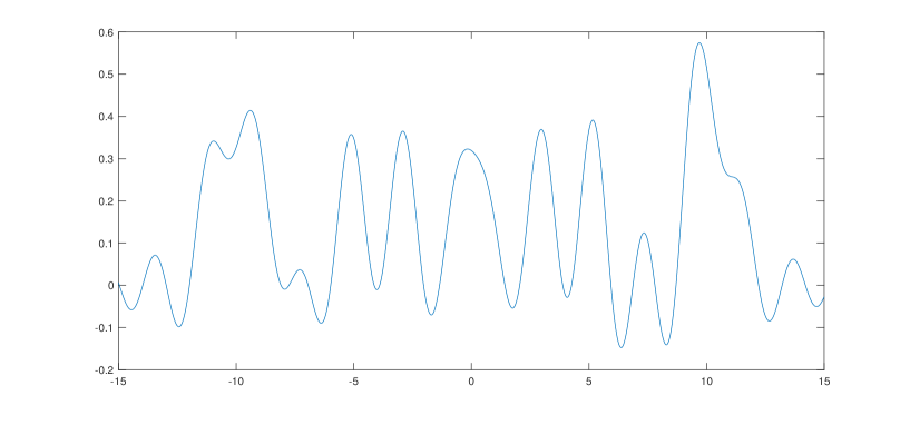
Figure 1. Test signal $f$ used in the numerical experiments.

The function $f$ shown in Fig 1 is used as the test signal throughout our numerical experiments. Further, we fix the parameters $\epsilon=\frac{1}{2}$ and $R=5$. As a result, the sampling interval $[-(1+3\epsilon)R,(1+3\epsilon)R]$ reduces to $\left[-\frac{25}{2},\frac{25}{2}\right]$, each sample $x_{i}$ is sampled according to the uniform distribution on $\left[-\frac{25}{2},\frac{25}{2}\right]$ and the finite dimensional approximation space is $V^{\left(1+\frac{5}{2}\epsilon\right)R}(g)=V^{\frac{45}{4}}(g)$.

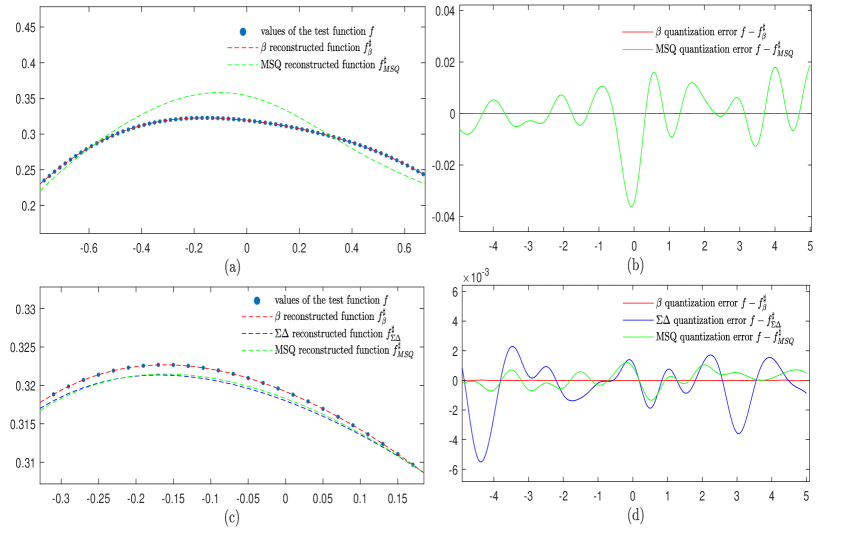
Figure 2. Panel (a) and (c): zoomed-in view of $f$ along with $f^{\sharp}$. Panel (b) and (d): error plots $f-f^{\sharp}$. The quantization alphabet for MSQ is taken as $\mathcal{A}_{10}$ and $\mathcal{A}_{80}$ (defined in (6.1)) for $L=10$ and $L=80$ respectively. For $\beta$ quantization, the greedy quantizer defined in Lemma 2.6 is used to quantize the samples. The noise transfer operator and the quantization alphabet are taken as $H_{\beta}=H_{5}$, i.e., $\beta=5$ and $\mathcal{A}^{0.1}_{10}$ for $L=10$, and $H_{20}$ and $\mathcal{A}^{1/130}_{80}$ for $L=80$, respectively. For the $\Sigma\Delta$ quantization scheme, the greedy quantizer defined in Lemma 2.6 is used to quantize the samples, with the noise transfer operator taken as $H=D^{7}$ and the quantization alphabet taken as $\mathcal{A}^{0.05}_{80}$.

We run our experiment in two parts. The whole process is carried out twice in each part, once with an alphabet of cardinality $20$ $(L=10)$ and once with an alphabet of cardinality $160$ $(L=80)$. When $L=10$, we use the MSQ and $\beta$ scheme for quantization and not the $\Sigma\Delta$ scheme. This is due to the fact that we employ the seventh-order $\Sigma\Delta$ greedy quantizer for $\Sigma\Delta$ quantization, which places constraints on the size of the alphabet (see Remark 5.3).

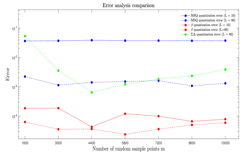
Figure 3. The quantizers and the quantization alphabets are the same as in Fig 2 for each of the three quantization schemes. We plot the reconstruction error along with the sample size $m$. For the $\Sigma\Delta$ and $\beta$ schemes $p$ is fixed as $200$.

Taking $3000$ random samples of the function $f$ from the interval $\left[-\frac{25}{2},\frac{25}{2}\right]$, in the first part (Fig 2), we show visually that we achieve good reconstruction using our method in both $\Sigma\Delta$ (seventh-order) and $\beta$ quantization schemes. We also plot the reconstructed function when using the MSQ scheme for comparison. In Fig 2(a) and 2(c), we plot a zoomed-in version of $f$ along with the reconstructed function $f^{\sharp}$. To better highlight the inaccuracy introduced by each of these three quantization procedures, we exhibit only the error introduced by each in Fig 2(b) and 2(d). Unlike the noise-shaping quantization approaches mentioned in this study, where the samples have to be partitioned into three collections due to the presence of the block diagonal matrix $V$, in the MSQ scenario as $p=m$ (which implies that $V$ is the identity matrix), no such partitioning is necessary. Further, the collection of symmetric Bernoulli random variables is also not required. For MSQ, we consider the quantization alphabet of the form

$$\mathcal{A}_{L}=\left\{-1+\frac{2n+1}{2L}:n\in\{0,\cdots,2L-1\}\right\},$$ (6.1)

with

$$q^{MSQ}_{i}:=\arg\min_{r\in\mathcal{A}_{L}}|f(x_{i})-r|\hskip 5.69046pt\forall\hskip 2.84544pti\in\{1,\cdots,m\}.$$

As discussed in the introduction, we apply a linear method for MSQ data: the function samples are quantized using the memoryless scalar quantizer, and then the canonical dual frame is operated on these quantized samples for reconstruction.

In the second part, Fig 3, we plot the average error $\left\|\left\{f(t_{i})-f^{\sharp}(t_{i})\right\}_{i=1}^{200}\right\|_{\infty}$ after five iterations. Here $\{t_{i}\}_{i=1}^{200}$ are evenly spaced points from $[-5,5]$. The following conclusions can be drawn from Fig 3. The $\beta$ scheme clearly outperforms both the $\Sigma\Delta$ scheme and MSQ. As expected, the MSQ error does not decrease with increasing sample size. The plot shows that for the considered sample range, MSQ performs slightly better than the $\Sigma\Delta$ scheme. The error in the $\Sigma\Delta$ scheme appears to decline at first; however, it levels out after a certain stage. The $\beta$ scheme exhibits similar behaviour, where increasing the number of samples does not result in further error decay after a certain point. One possible explanation for why, in neither case, we observe continued decay could be that the theorem statement requires us to increase the sampling interval as the sample size increases, which we do not do due to computational difficulties. So, there may be some inherent limitations related to the fact that the projection error $\|f-Pf\|_{L^{2}[-5,5]}$ does not decrease with increasing samples. However, it is also possible that the error will continue to reduce slowly as the sample size grows, but computational constraints prevent us from using more samples.

At the same time, the $\beta$ scheme also performs significantly better in terms of computation speed than the MSQ and the $\Sigma\Delta$ schemes. Potential reasons for that are that in MSQ, one works with considerably larger frames, necessitating more computations to calculate the dual frame, and in the $\Sigma\Delta$ scheme, the function samples must be quantized using a seventh-order $\Sigma\Delta$ quantizer, which is computationally intensive.

Remark 6.1.

We remark that $\Sigma\Delta$ quantization falls short of $\beta$ quantization and also MSQ both in terms of accuracy and computational performance. We nevertheless decided to include the method in our discussion, as it has performed quite successfully in other contexts and hence is a natural candidate for a reconstruction approach. We consider it to be an interesting observation that it should not be the method of choice in this scenario.

7. Concluding remarks

In this paper, we established a first error analysis for reconstruction from quantized random samples of bandlimited signals both in the case of $\Sigma\Delta$ and distributed noise-shaping quantization. Our theoretical findings suggest an advantage of the latter approach, which we also observed in our numerical experiments.

We see a number of interesting directions to explore our findings further.

• In this paper, we consider the three-bin scenario, in which the sample points $\{x_{i}\}_{i=1}^{m}$ are divided into three collections (bins). We are confident that by increasing the number of bins, our error decay rate will improve.

• Random sampling techniques were primarily developed to address the issues that arise when sampling multivariate functions. While we consider the quantization of bandlimited functions defined on $\mathbb{R}$ in this paper, we believe the results can be extended to higher dimensions with similar techniques.

• In the method presented in this study, function samples can only be quantized after they have all been collected and stored. We want to improve this technique further by creating a new on-line approach in which samples are quantized in real-time during the process of collection.

• Finally, as stated in the introduction, the sampling interval increases as the number of samples grows in both of our main results. We wish to improve on this by developing an algorithm in which the error decreases with increasing sample size but does not require a corresponding increase in the sampling interval.

References

[1]
A. Aldroubi and K. Gröchenig, Nonuniform sampling and reconstruction
in shift-invariant spaces, SIAM Rev. 43 (2001), no. 4, 585–620.
MR 1882684
[2]
S. Arati, P. Devaraj, and A. K. Garg, Random average sampling and
reconstruction in shift-invariant subspaces of mixed Lebesgue spaces,
Results Math. 77 (2022), no. 6, Paper No. 223, 38. MR 4491129
[3]
R. F. Bass and K. Gröchenig, Random sampling of multivariate
trigonometric polynomials, SIAM J. Math. Anal. 36 (2004/05), no. 3,
773–795. MR 2111915
[4]
by same author, Random sampling of bandlimited functions, Israel J. Math.
177 (2010), 1–28. MR 2684411
[5]
by same author, Relevant sampling of band-limited functions, Illinois J. Math.
57 (2013), no. 1, 43–58. MR 3224560
[6]
J. J. Benedetto, A. M. Powell, and Ö. Yilmaz, Second-order
sigma-delta quantization of finite frame expansions,
Appl. Comput. Harmon. Anal. 20 (2006), no. 1, 126–148. MR 2200933
[7]
by same author, Sigma-delta quantization and finite frames,
IEEE Trans. Inform. Theory 52 (2006), no. 5, 1990–2005.
MR 2234460
[8]
J. Blum, M. Lammers, A. M. Powell, and Ö. Yilmaz, Sobolev duals in
frame theory and sigma-delta quantization, J. Fourier Anal. Appl.
16 (2010), no. 3, 365–381. MR 2643587
[9]
B. G. Bodmann and V. I. Paulsen, Frame paths and error bounds for
sigma-delta quantization, Appl. Comput. Harmon. Anal. 22 (2007),
no. 2, 176–197. MR 2295294
[10]
B. G. Bodmann, V. I. Paulsen, and S. A. Abdulbaki, Smooth frame-path
termination for higher order sigma-delta quantization, J. Fourier Anal.
Appl. 13 (2007), no. 3, 285–307. MR 2334611
[11]
E. J. Candès, J.K. Romberg, and T. Tao, Robust uncertainty principles:
exact signal reconstruction from highly incomplete frequency information,
IEEE Trans. Inform. Theory 52 (2006), no. 2, 489–509. MR 2236170
[12]
by same author, Stable signal recovery from incomplete and inaccurate
measurements, Comm. Pure Appl. Math. 59 (2006), no. 8, 1207–1223.
MR 2230846
[13]
E. Chou and C. S. Güntürk, Distributed noise-shaping
quantization: I. Beta duals of finite frames and near-optimal
quantization of random measurements, Constr. Approx. 44 (2016),
no. 1, 1–22. MR 3514402
[14]
by same author, Distributed noise-shaping quantization: II. Classical
frames, Excursions in harmonic analysis. Vol. 5, Appl. Numer. Harmon.
Anal., Birkhäuser/Springer, Cham, 2017, pp. 179–198. MR 3699683
[15]
E. Chou, C. S. Güntürk, F. Krahmer, R. Saab, and Ö. Yilmaz,