A large-scale magnetic field via $\alpha\Omega$ dynamo in binary neutron star mergers

Abstract

The merger of neutron stars drives a relativistic jet which can be observed as a short gamma-ray burst [2, 1, 3, 4]. A strong large-scale magnetic field is necessary to launch the relativistic jet [5]. However, the magnetohydrodynamical mechanism to build up this magnetic field remains uncertain. Here we show that the $\alpha\Omega$ dynamo mechanism driven by the magnetorotational instability [6, 7] builds up the large-scale magnetic field inside the long-lived binary neutron star merger remnant by performing an ab initio super-high resolution neutrino-radiation magnetohydrodynamics merger simulation in full general relativity. As a result, the magnetic field induces the Poynting-flux dominated relativistic outflow with the luminosity $\sim 10^{51}$ erg/s and magnetically-driven post-merger mass ejection with the mass $\sim 0.1M_{\odot}$. Therefore, the magnetar scenario in binary neutron star mergers is possible [8]. These can be the engines of short-hard gamma-ray bursts and very bright kilonovae. Therefore, this scenario is testable in future observation.

K. Kiuchi(Max Planck Institute for Gravitational Physics, CGQPI-YITP), A. Reboul-Salze(Max Planck Institute for Gravitational Physics), Masaru Shibata(Max Planck Institute for Gravitational Physics, CGPQI-YITP), Yuichiro Sekiguchi (Toho Univ.)

The observation of GW170817/GRB 170817A/AT 2017gfo made binary neutron star mergers a leading player of multi-messenger astrophysics [9, 1]. It revealed that at least a part of the origin of short-hard gamma-ray bursts and the heavy elements via the rapid-neutron capture process ($r$-process) is binary neutron star mergers [2, 1, 3, 4, 10, 11, 12, 13].

All the fundamental interactions play an essential role in binary neutron star mergers. Thus, to theoretically explore them, a numerical-relativity simulation implementing all the effects of the fundamental interactions is the chosen way. Numerical relativity simulations manage to qualitatively explain AT 2017gfo, i.e., the kilonova emissions associated with the radioactive decay of the $r$-process elements [14, 15, 16, 17, 18, 19, 20, 21, 22, 23, 24]. However, a quantitative understanding of it is on its way. Moreover, there is no theoretical consensus about how the binary neutron star merger drove the short-hard gamma-ray burst [25, 5, 26].

A relativistic jet was launched from the binary neutron star merger and was observed as a short-hard gamma-ray burst [2, 1, 3, 4]. Such relativistic jets are most likely driven by a magnetohydrodynamics process. This indicates that a binary neutron star merger remnant must build up a large-scale magnetic field via the dynamo to launch the jet [6]. However, the mechanism of the large-scale dynamo in the merger remnant still needs to be clarified [27, 28]. We tackle this problem with a super-high resolution neutrino-radiation magnetohydrodynamics simulation of a binary neutron star merger in full general relativity.

We employ our latest version of numerical-relativity neutrino-radiation magnetohydrodynamics code [29]. We employ a static mesh refinement with 2:1 refinements to cover a wide dynamic range. For the simulations in this article, the grid structure consists of sixteen Cartesian domains, and each domain has a $2N\times 2N\times N$ grid in the $x,y$, and $z$-directions where we assume the orbital plane symmetry. We set $N=361$ and $\Delta x_{\rm finest}=12.5$ m. The employed grid resolution is the highest among the binary neutron star merger simulations [30]. The initial orbital separation is $\approx 44$ km (see Methods).

We employ DD2 [31] as an equation of state for the neutron star matter and symmetric binary with a total mass of $2.7M_{\odot}$. With this setup, a hypermassive neutron star transiently formed after the merger will survive for $>O(1)$ s [32].

The purely poloidal magnetic-field loop is embedded inside the neutron stars with a maximum field strength of $B_{0,\mathrm{max}}=10^{15.5}$ G [33]. Although it is much stronger than those observed in binary pulsars of $10^{7}$–$10^{11}$ G [34], it is natural to anticipate that the magnetic-field amplification leads to a high field strength ($>10^{16}$ G) in a short timescale after the merge in reality (see below).

Figure 1 plots the evolution of electromagnetic energy as a function of the post-merger time. As reported in Refs. [35, 30], the electromagnetic energy is exponentially amplified shortly after the merger due to the Kelvin-Helmholtz instability, which emerges at the contact interface when the binary merges. In the inset, we generate the same plot for $-1\leq t-t_{\mathrm{merger}}\leq 5$ ms but different initial magnetic-field strengths of $B_{0,\mathrm{max}}=10^{15}$ G with red and $B_{0,\mathrm{max}}=10^{14}$ G with orange while keeping the grid resolution. Also, we plot the results for the other grid resolutions of $\Delta x_{\rm finest}=100$ m and $200$ m for the brown and purple curves, respectively, while keeping $B_{0,\mathrm{max}}=10^{15.5}$ G. It clearly shows that the magnetic-field amplification for $0\lesssim t-t_{\mathrm{merger}}\lesssim 1$ ms does not depend on the employed initial field strength but on the employed grid resolution as expected from the properties of the Kelvin-Helmholtz instability [36, 37] (see Extended Data Figure 1).

At $t-t_{\mathrm{merger}}\approx 5$ ms, the electromagnetic energy temporarily settles to $\approx 3\times 10^{50}$ erg. By this time, the shock waves generated by the collision of the two neutron stars dissipate the shear layer. However, the toroidal magnetic field (dotted curve) is subsequently amplified. In particular, its contribution to the total electromagnetic energy becomes prominent for $t-t_{\mathrm{merger}}\gtrsim 20$ ms and the growth rate is proportional to $t^{2}$, which indicates that an efficient magnetic winding occurs with a coherent poloidal magnetic field [38]. We confirm that the contribution to the winding originating from the initial coherent poloidal magnetic field is sub-dominant, as plotted for the simulation with $\Delta x_{\rm finest}=200$ m in Fig. 1. With this resolution, it is hard to resolve the Kelvin-Helmholtz and magnetorotational instability (see Extended Data Figure 1 and Extended Data Figure 5). Thus, the compression at the merger and subsequent winding amplify the magnetic field, which could be an artifact due to the initial strong magnetic field. However, there is a striking difference, particularly in the poloidal magnetic field, between the simulations with $\Delta x_{\rm finest}=12.5$ m and $\Delta x_{\rm finest}=200$ m. Because the magnetic field amplified via the Kelvin-Helmholtz instability is randomly oriented [30], there should be a mechanism to generate the coherent poloidal magnetic field.

The $\alpha\Omega$ dynamo driven by the magnetorotational instability [39] in the current context is a potential mechanism to generate the large-scale magnetic field [6, 7]. In the mean-field dynamo theory, we assume that the physical quantity $Q$ is composed of the mean field $\bar{Q}$ and the fluctuation $q$, i.e., $Q=\bar{Q}+q$. With it, we cast the induction equation into

$$\partial_{t}\bar{\bf{B}}=\nabla\times\left(\bar{\bf{U}}\times\bar{\bf{B}}+\bar{\bf{\cal E}}\right),$$ (1)

where $\bar{\bf{\cal E}}=\overline{\bf{u}\times\bf{b}}$ is the electromotive force due to the fluctuations, $\bf{B}=\bar{\bf{B}}+\bf{b}$ is the magnetic field, and $\bf{U}=\bar{\bf{U}}+\bf{u}$ is the velocity field. Note that the magnetorotational instability-driven turbulence produces the fluctuation $\bf{u}$ and $\bf{b}$. In the $\alpha\Omega$ dynamo, we express the electromotive force as a function of the mean magnetic field,

$$\bar{\cal E}_{i}=\alpha_{ij}\bar{B}_{j}+\beta_{ij}\left(\overline{\nabla\times\bar{B}}\right)_{j},$$ (2)

where $\alpha_{ij}$ and $\beta_{ij}$ are tensors that do not depend on $\bar{B}_{j}$. We calculate the mean field by taking the average in the azimuthal direction.

In the presence of a cylindrical differential rotation, the simplest mean field dynamo is an $\alpha\Omega$ dynamo, where the toroidal magnetic field is generated by the shear of the poloidal magnetic field by the differential rotation $\bar{U}_{\phi}$, also called $\Omega$ effect. The decreasing rotation with radius and Eq. (1) implies that the $\bar{B}_{\phi}$ should be anti-correlated with $\bar{B}_{R}$. To complete the dynamo cycle, the poloidal magnetic field has to be generated by the toroidal electromotive force $\bar{\cal E}_{\phi}$ with a main contribution from a diagonal component, $\alpha_{\phi\phi}$; the so-called $\alpha$ effect. $\bar{\cal E}_{\phi}$ is therefore correlated/anti-correlated to $\bar{B}_{\phi}$, depending on the sign of $\alpha_{\phi\phi}$ (Eq. (2)). This complete cycle forms a dynamo wave that oscillates with a period of $P_{\mathrm{theory}}=2\pi\lvert\frac{1}{2}\alpha_{\phi\phi}\frac{d\Omega}{d\ln R}k_{z}\rvert^{-1/2}$ [6, 7] and propagates in the direction of $\alpha_{\phi\phi}\nabla\Omega\times e_{\phi}$, according to the Parker-Yoshimura rule [40, 41]. Here $k_{z}$ is the wave number of the dynamo wave in the vertical direction. In this theoretical description, we have supposed that contributions from the other $\alpha_{ij}$ components and the turbulent resistivity tensor $\beta_{ij}$ are sub-dominant. We will show that it is the case in the following.

First, we confirm that the employed simulation setup can capture the fastest-growing mode of the magnetorotational instability in the outer region of the hypermassive neutron star (see Extended Data Figure 5). Therefore, the turbulent state is developed. Figure 2 plots the butterfly diagram for $\bar{B}_{\phi}$, $\bar{B}_{R}$, and $\bar{\cal E}_{\phi}$. As a representative radius, we select $R=30$ km. The top-left and right panels show the anti-correlation between $\bar{B}_{\phi}$ and $\bar{B}_{R}$, which indicates the $\Omega$ effect. To quantify the correlation between $\bar{B}_{\phi}$ and $\bar{\mathcal{E}}_{\phi}$, we compute the Pearson correlation $C_{P}(X,Y)$ between the two quantities, $X$ and $Y$, in the bottom-right panel of Fig. 2. This figure shows that $\bar{B}_{\phi}$ and $\bar{\mathcal{E}}_{\phi}$ anti-correlate for $z\lesssim 15$ km, where the pressure scale height at $R=30$ km is $\approx 14.6$ km. The correlation between the electromotive force and mean current $\bar{J}_{i}=\left(\overline{\nabla\times\bar{B}}\right)_{i}$ is small, and thus, the $\beta_{ij}$ tensor can be neglected (see Extended Data Figure 2). Therefore, the generation of the mean poloidal magnetic field is determined primarily by the $\alpha_{ij}$ tensor. While $\alpha_{\phi R}$ has a non-negligible contribution, the contribution of $\alpha_{\phi\phi}B_{\phi}$ dominates in the turbulent region for $z\lesssim 10$ km (see Extended Data Figure 3). This shows that $\alpha_{\phi\phi}$ is the main component, which is plotted in the bottom-right panel of Fig. 2.

With these quantities, we can predict the period of the $\alpha\Omega$ dynamo listed in Table 1, where we measure the shear rate $q=-d\ln\Omega/d\ln R$ at the selected radius and choose the wave number $k_{z}$ corresponding to the pressure scale height, the most extended vertical length in the turbulent region. The sixth and seventh columns report the predicted period of the $\alpha\Omega$ dynamo and the period measured in the butterfly diagram. The agreement at $R=30$ km is remarkable. We also show the comparison at different radii from $R=20$ km to $R=50$ km in the table, and the deal is also reasonable. In addition, since $\alpha_{\phi\phi}$ is negative and $q$ is positive, the dynamo wave propagates along the direction of the Parker-Yoshimura rule, i.e., the $z$-direction.

With these findings, we conclude that the dynamo in our simulation can be interpreted as an $\alpha\Omega$ dynamo, and it builds up the large-scale magnetic field in the remnant hypermassive neutron star (see Fig. 1).

After the development of the coherent poloidal magnetic field due to the $\alpha\Omega$ dynamo and resultant efficient magnetic winding, a magnetic-tower outflow is launched toward the polar direction (http://www2.yukawa.kyoto-u.ac.jp/~kenta.kiuchi/anime/SAKURA/DD2_135_135_Dynamo.mp4, see Methods). We confirm that the contribution of the winding due to the initial coherent poloidal magnetic field to the Poynting flux-dominated outflow and the post-merger ejecta is minor (see Extended Data Figure 7).

The luminosity of the Poynting flux defined by $L_{\mathrm{Poy}}=-\oint_{r\approx 500~{}\mathrm{km}}\sqrt{-g}\left({T^{r}}_{t}\right)_{\mathrm{(EM)}}d\Omega$, where $T^{\mu\nu}_{\mathrm{(EM)}}$ is the stress energy tensor for the electromagnetic field, is $\approx 10^{51}$ erg/s at the end of the simulation of $t-t_{\mathrm{merger}}\approx 150$ ms. The high Poynting flux is confined in the region with $\theta\lesssim 12^{\circ}$ where $\theta$ is a polar angle as plotted in the top-left panel of Fig. 3 (see also Extended Data Figure 7). The luminosity and jet opening angle are compatible with observed short-hard gamma-ray bursts [42].

The dynamical ejecta driven by the tidal force and the shock wave during the merger phase is $\approx 0.002M_{\odot}$ [43]. After the development of the coherent magnetic field, we observe a new component in the ejecta driven by the Lorentz force, i.e., the magnetically-driven wind [44]. The mass of this component is $\approx 0.1M_{\odot}$ at the end of the simulation $t-t_{\mathrm{merger}}\approx 150$ ms. The electron fraction of the post-merger ejecta shows a peak around $\approx 0.2$ with an extension to $\sim 0.5$. The terminal velocity of the post-merger ejecta peaks around $\approx 0.08c$ where $c$ is the speed of light. Therefore, it could contribute to a bright kilonova emission via the synthesis of $r$-process heavy elements [8, 45].

We speculate that the high luminosity state and the post-merger mass ejection would continue for $O(1)$ s which corresponds to the neutrino cooling timescale [46, 47]. As reported in Refs. [32, 48], the envelope expands due to the angular momentum transport facilitated by the magnetorotational instability-driven turbulent viscosity after the neutrino cooling becomes inefficient. As a result, the funnel region above the remnant neutron star expands and the jet could no longer be collimated. A long-term simulation for $O(1)$ s of a remnant massive neutron star is future work to be pursued. Also, a simulation with initially weakly magnetized binary neutron stars is necessary to confirm the picture reported in this article because the saturated magneto-turbulent state and the generation timescale of the coherent poloidal magnetic field due to the magnetorotational instability could depend on the initial magnetic field strength and flux [49].

To summarize, we tackled the large-scale magnetic-field generation in the long-lived binary neutron star merger remnant by the super-high resolution neutrino-radiation magnetohydrodynamics simulation in general relativity. The magnetorotational instability-driven $\alpha\Omega$ dynamo generates the large-scale magnetic field. As a result, the launch of the Poynting-flux-dominated relativistic outflow in the polar direction and an enormous amount of magnetically-driven wind are induced. Our simulation suggests that the magnetar engine generates short-hard gamma-ray bursts and bright kilonovae emission, which could be observed in the near-future multi-messenger observations.

Table 1: The $\alpha\Omega$ dynamo period prediction and simulation data at several radii

$R$ (km)	$\alpha_{\phi\phi}$ (cm/s)	$\Omega$ (rad/s)	Shear rate	$k_{z}$ (/cm)	$P_{\mathrm{theory}}$ (s)	$P_{\mathrm{sim}}$ (s)
$20$	$-8.1\times 10^{6}$	$4025$	$q=-1.0$	$6.3\times 10^{-6}$	$0.020$	$0.018$
$30$	$-1.0\times 10^{7}$	$2515$	$q=-1.34$	$4.2\times 10^{-6}$	$0.021$	$0.018$–$0.024$
$40$	$-1.0\times 10^{7}$	$1688$	$q=-1.44$	$3.3\times 10^{-6}$	$0.037$	$0.018$–$0.030$
$50$	$-4.4\times 10^{6}$	$1200$	$q=-1.50$	$2.6\times 10^{-6}$	$0.062$	$0.030$–$0.040$

$P_{\mathrm{theory}}$: The $\alpha\Omega$ dynamo period, $P_{\mathrm{sim}}$: Butterfly diagram period in the simulation

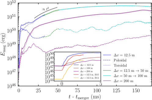
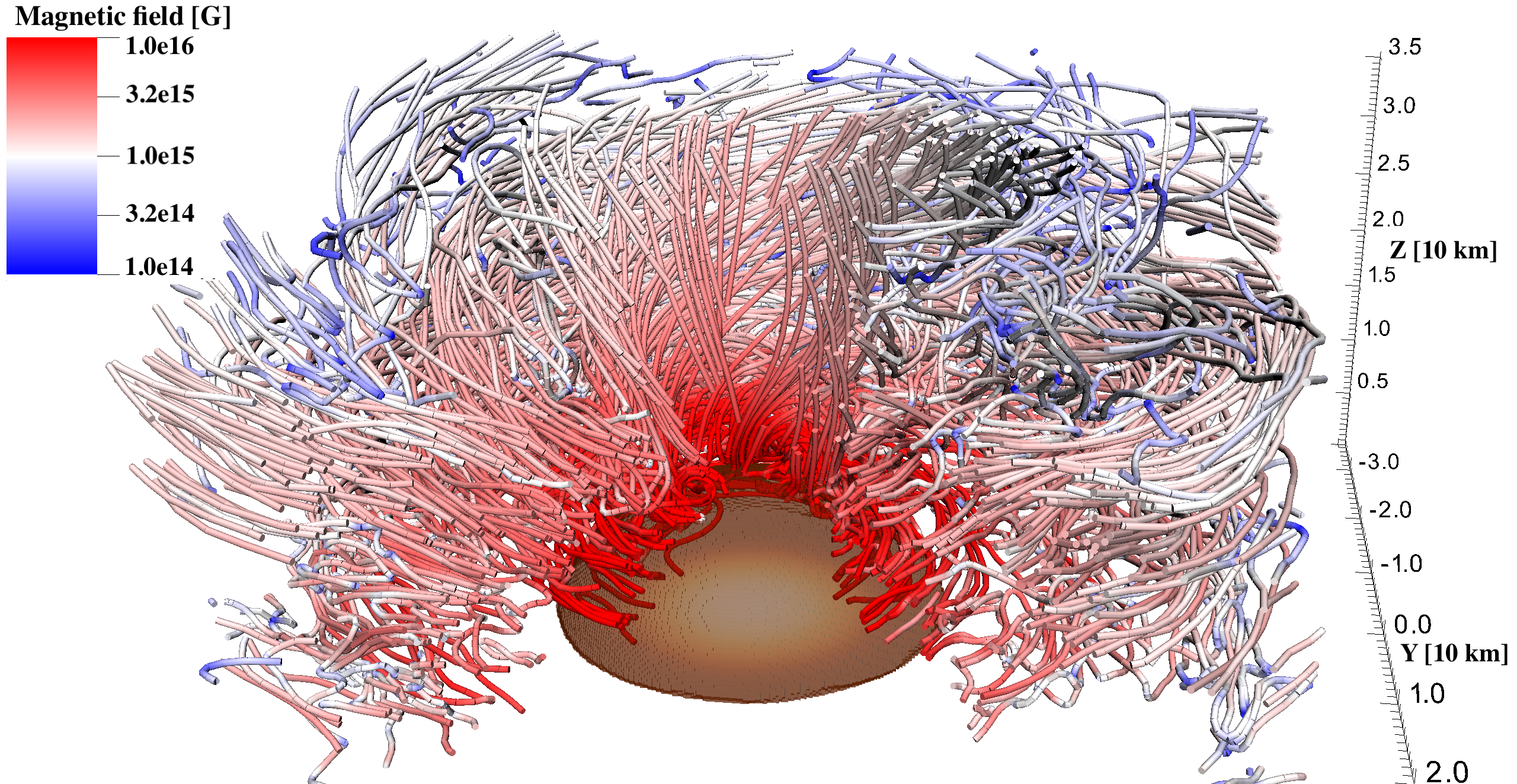
Figure 1: Overview of the magnetic field evolution in the binary neutron star merger remnant. (Top) Electromagnetic energy as a function of the post-merger time for the total (solid), the poloidal (dashed), and the toroidal (dotted) components. The purple curves are for the simulation with $\Delta x_{\rm finest}=200$ m. The inset shows how the magnetic field amplification due to the Kelvin-Helmholtz instability depends on the initial magnetic-field strength and employed grid resolution. (Bottom) Magnetic field lines for the density of $\rho<10^{13}$ g cm^-3 at $t-t_{\mathrm{merger}}\approx 130$ ms. The core of the hypermassive neutron star is shown for the density of $\rho>10^{13}$ g cm^-3.

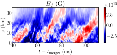
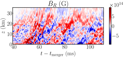
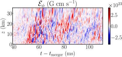
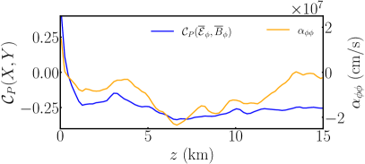
Figure 2: $\alpha\Omega$ dynamo inside the binary neutron star merger remnant. Butterfly diagram at $R=30$ km: (Top-left) Mean toroidal magnetic field $\bar{B}_{\phi}$. (Top-right) Mean radial magnetic field $\bar{B}_{R}$. (Bottom-left) Toroidal electromotive force $\bar{\mathcal{E}}_{\phi}$. (Bottom-right) $\alpha_{\phi\phi}$ parameters (orange) and correlation between $\bar{\mathcal{E}}_{\phi}$ and $\bar{B}_{\phi}$ (blue).

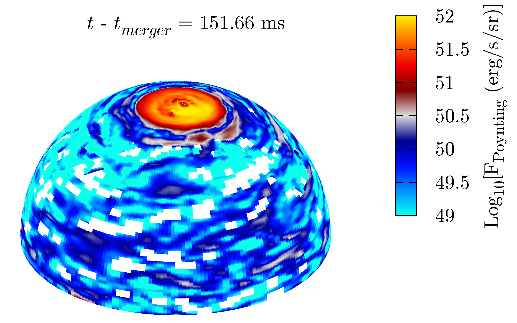
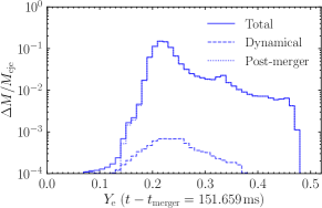
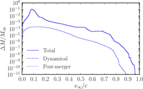
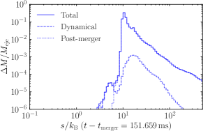
Figure 3: The electromagnetic signals from the binary neutron star merger remnants. (Top-left) Angular distribution of the Poynting flux on a sphere with $r\approx 500$ km at $t-t_{\mathrm{merger}}\approx 150$ ms. (Top-right) The electron fraction distribution for the magnetically-driven post-merger ejecta (dashed) and the dynamical ejecta (dotted). (Bottom) Same as the top-right panel, but for the terminal velocity (left) and entropy per baryon (right).

0.1 Numerical method

Our code implements the Baumgarte-Shapiro-Shibata-Nakamura-puncture formulation to solve Einstein’s equation [50, 51, 52, 53]. The code also employs the Z4c prescription to suppress the constraint violation [54]. The fourth-order accurate finite difference is used as a discretization scheme in space and time. The sixth-order Kreiss-Oliger dissipation is also employed. The HLLD Riemann solver [55] and the constrained transport scheme [56] are employed to solve the equations of motion of the relativistic magnetohydrodynamic fluid. The neutrino-radiation transfer is solved by the gray M1+GR-Leakage scheme [57] to take into account neutrino cooling and heating.

0.2 Initial data

We employ quasi-equilibrium initial data of irrotational binary neutron stars in the neutrino-free beta equilibrium derived in a previous paper [32] using the public spectral library LORENE [58]. The initial orbital angular velocity is $Gm_{0}\Omega_{0}/c^{3}\approx 0.028$ with $m_{0}=2.7M_{\odot}$, and the residual orbital eccentricity is $\approx 10^{-3}$. For our high-resolution study, the data is remapped onto the computational domain described in the section of Grid setup.

0.3 Grid setup

We employ the static mesh refinement with 2:1 refinement, i.e., a grid resolution of a coarser domain is twice that of a finer domain. All the domains are composed of concentric Cartesian domains with a fixed grid number $N$. The grid number is $2N\times 2N\times N$ in the $x$, $y$, and $z$-directions where we assume the orbital plane symmetry. We employ the sixteen domains with $N=361$ and the finest grid resolution of $\Delta x_{\rm finest}=12.5$ m. The first three finest domains whose size are $[-4.5:4.5~{}{\rm km}]^{2}\times[0:4.5~{}{\rm km}]$, $[-9:9~{}{\rm km}]^{2}\times[0:9~{}{\rm km}]$, and $[-18:18~{}{\rm km}]^{2}\times[0:18~{}{\rm km}]$, respectively, are employed to resolve the Kelvin-Helmholtz instability, which emerges on a contact interface (shear layer) when the two neutron stars merge. The initial binary separation is $\approx 44$ km, and the coordinate radius of the neutron star is $10.9$ km. Thus, the fourth finest domain with $[-36:36~{}{\rm km}]^{2}\times[0:36~{}{\rm km}]$ covers the entire binary neutron star.

We start a simulation with $\Delta x_{\rm finest}=12.5$ m and sixteen static mesh refinement domains. At $\approx 30$ ms after the merger, we remove the two finest domains with $\Delta x_{\rm finest}=12.5$ m and $\Delta x=25$ m and continue the simulation with $\Delta x_{\rm finest}=50$ m until $\approx 50$ ms after the merger. Then, we remove the domain with $\Delta x_{\rm finest}=50$ m and continue the simulation with $\Delta x_{\rm finest}=100$ m. This strategy allows capturing the efficient magnetic-field amplification via the Kelvin-Helmholtz instability and resolving the magnetorotational instability inside the remnant while saving computational costs. For the convergence test, we also perform the simulations with $\Delta x_{\rm finest}=100(200)$ m and $N=361(185)$. The number of domains is thirteen.

0.4 Equation of state

We extend an original DD2 equation of state to the low-density and temperature region with the Helmholtz equation of state [59]. Because any high-resolution shock-capturing scheme does not allow the vacuum state, we employ the atmospheric prescription outside the neutron stars. Specifically, we set the constant atmospheric density of $10^{3}~{}\mathrm{g/cm^{3}}$ inside $r\leq L_{\mathrm{atm}}$, and assume the power-law profile with $\rho_{\mathrm{atm}}=\mathrm{max}[10^{3}(L_{\mathrm{atm}}/r)^{3}~{}\mathrm{g/cm^{3}},\rho_{\mathrm{fl}}]$ for r$>L_{\mathrm{atm}}$ where we set $L_{\mathrm{atm}}=36$ km. The employed DD2 equation of state determines the floor value of the rest-mass density, which is $\rho_{\mathrm{fl}}=0.167~{}\mathrm{g/cm^{3}}$. We also assume the constant atmospheric temperature of $10^{-3}$ MeV.

0.5 Kelvin-Helmholtz instability

The top panel of Extended Data Figure 1 is the same as the inset in Fig. 1 in the main article but with additional data. The blue, brown, and purple-solid curves plot the results with $\Delta x_{\rm finest}=12.5$ m, $100$ m, and $200$ m, respectively, with $B_{0,\mathrm{max}}=10^{15.5}$ G. The red- and orange-solid curves show the results with $\Delta x_{\rm finest}=12.5$ m with $B_{0,\mathrm{max}}=10^{15}$ G and $10^{14}$ G, respectively. The cyan curve shows the result with $\Delta x_{\rm finest}=18.75$ m and $B_{0,\mathrm{max}}=10^{14}$ G. The blue- and red-dotted curves plot the result with $\Delta x_{\rm finest}=12.5$ m and $B_{0,\mathrm{max}}=10^{14}$ G magnified by the square of the ratio of the initial magnetic-field strength, i.e., $(10^{15.5}/10^{14})^{2}=10^{3}$ and $(10^{15}/10^{14})^{2}=10^{2}$, respectively.

This figure suggests the following two points: The blue(red)-solid and -dotted curves overlap until the back reaction starts to activate, which happens when the electromagnetic energy reaches $\approx 3\times 10^{49}$ erg. This implies that the magnetic field is passive for $t-t_{\mathrm{merger}}\lesssim 1$ ms, i.e., the linear phase. The saturation of the electromagnetic energy via the Kelvin-Helmholtz instability is likely to be $\approx 1$–$3\times 10^{50}$ erg corresponding to $O(0.1)\%$ of the internal energy [35]. The second point is that the growth rate of the electromagnetic energy in the linear phase is determined by the employed grid resolution, not by the employed initial magnetic field strength. To quantify the growth rate dependence on the grid resolution and initial magnetic-field strength, we estimate the growth rate by fitting the electromagnetic energy as $E_{\mathrm{mag}}(t)=A\exp\left(\sigma_{\mathrm{KH}}(t-t_{\mathrm{merger}})\right)$ for $0\lesssim t-t_{\mathrm{merge}}\lesssim 1$ ms, which corresponds to the linear phase. The bottom panel of Extended Data Figure 1 plots the estimated growth rate as a function of the initial magnetic-field strength. The symbols denote the employed grid resolutions. With $\Delta x_{\rm finest}=12.5$ m, the growth rate is $\approx 7~{}\mathrm{ms}^{-1}$, irrespective of the initial magnetic-field strength. The growth rate increases with the grid resolution. With $\Delta x_{\rm finest}=100$ and 200 m, the efficient amplification cannot be captured. All the properties are consistent with those of the Kelvin-Helmholtz instability, i.e., the smaller the scale of the vortices is, the larger the growth rate is [62]. The reality is located in the left-top direction in this diagram, i.e., the weak magnetic field observed in binary pulsars and infinitesimal grid resolution. Therefore, we anticipate that the electromagnetic energy will saturate in a very short timescale, $\ll 1$ ms after the merger, in binary neutron star mergers, irrespective of the magnetic-field strength at the onset of the merger unless a black hole is promptly formed [35, 60, 61].

0.6 $\alpha\Omega$ dynamo

To understand the dynamo process in the simulation, we use the framework of the mean field theory with an axisymmetric mean. We present in this section the complementary analysis of the other contributions to the generation of the mean magnetic field than the $\alpha_{\phi\phi}$-effect and $\Omega$-effect. We therefore show in this section the other correlations between the electromotive force and the magnetic field and the estimated values of the alpha tensor. The correlations are computed according to the Pearson correlation coefficient between two quantities $X$ and $Y$ with the following formula:

$$\mathcal{C}_{P}(X,Y)=\frac{\int_{t}(X-\langle X\rangle_{t})(Y-\langle Y\rangle_{t})dt}{\sqrt{(\int_{t}(X-\langle X\rangle_{t})^{2}dt)}\sqrt{(\int_{t}(Y-\langle Y\rangle_{t})^{2}dt)}},$$ (3)

where $\langle\cdot\rangle_{t}$ represents a time average. Since the correlations between the mean current $\bar{J}_{i}$ and the electromotive force (see Extended Data Figure 2) are lower than the the correlations between the mean magnetic field $\bar{B}_{i}$ (see left panel of Extended Data Figure 3 and Extended Data Figure 4), we neglect the contribution of the mean current and consider only the contributions from the mean magnetic field.

For the values of the alpha tensor components, several methods can be used. The simplest one is to estimate from the correlation but this method assumes that one component is dominant. In order to take into account the off-diagonal contributions, we compute the values of the alpha tensor coefficients in this study by using the singular value decomposition method to perform the least-square fit of mean-current data and mean field [63].

0.7 Generation of the mean poloidal field $\bar{B}_{R}$

The generation of the axisymmetric poloidal field is due to the curl of the toroidal component of the electromotive force in the averaged induction equation. In this section, we show the non-diagonal correlations and the diagonal ones between the toroidal electromotive force and magnetic field components (Extended Data Figure 3). The correlations with the toroidal component of the electromotive force show that the radial magnetic field is correlated as well. This can be explained as the radial field $\bar{B}_{R}$ is anti-correlated to the toroidal magnetic field $\bar{B}_{\phi}$ due to the $\Omega$-effect. Because the toroidal field is correlated to the toroidal electromotive force, the radial field is also correlated to it. To confirm this picture, we compare the time-averaged values of $\alpha_{\phi\phi}\bar{B}_{\phi}$ and $\alpha_{\phi R}\bar{B}_{R}$ in the first $10$ km and find

$$\frac{\langle\alpha_{\phi\phi}\bar{B}_{\phi}\rangle_{t}}{\langle\alpha_{\phi R}\bar{B}_{R}\rangle_{t}}=1.87.$$ (4)

The generation of the poloidal field is therefore dominated by the diagonal $\alpha$-effect, while there is an off-diagonal contribution of the mean radial field.

0.8 Generation of the mean toroidal field

For the generation of the toroidal magnetic field, we can verify whether the dynamo is an $\alpha\Omega$ dynamo or an $\alpha^{2}\Omega$ dynamo by looking at the correlations between the poloidal electromotive force and the magnetic field (see Extended Data Figure 4) and estimating the values of the corresponding alpha tensor components. Some components, for example the mean toroidal field $\bar{B}_{\phi}$, are strongly correlated with the radial component of the electromotive force. This raises the question of whether the alpha effect contributes to generating the mean toroidal field. The dynamo would be therefore an $\alpha^{2}\Omega$ dynamo rather than a $\alpha\Omega$ dynamo. To distinguish between these two dynamos, we estimated the ratio of the two dynamo numbers $C_{\alpha}=\max(\lvert\alpha_{Ri}\rvert,\lvert\alpha_{zi}\rvert)R/\eta$ for $i\in[R,\phi,z]$ and $C_{\Omega}=\Omega R^{2}/\eta$, where $\eta$ is the resistivity, in the turbulent region averaged for one scale height, which gives at $R=30$ km

$$\frac{C_{\Omega}}{C_{\alpha}}=\frac{\Omega R}{\max(\lvert\alpha_{Ri}\rvert,\lvert\alpha_{zi}\rvert)}\approx 30.8$$ (5)

The $\alpha$ effect that generates the toroidal field can therefore reasonably be neglected as the $\Omega$-effect dominates the generation of the mean toroidal field.

0.9 Magnetorotational instability, neutrino viscosity, and neutrino drag

To quantify how well the magnetorotational instability is resolved in our simulation, we estimate the rest-mass-density-conditioned magnetorotational instability quality factor defined by

$$\langle Q_{\mathrm{MRI}}\rangle_{\rho}\equiv\frac{\langle\lambda_{\mathrm{MRI}}\rangle_{\rho}}{\Delta x}=\frac{1}{\Delta x}\frac{\int_{\rho}\lambda_{\mathrm{MRI}}d^{3}x}{\int_{\rho}d^{3}x},$$ (6)

where $\lambda_{\mathrm{MRI}}=2\pi B^{z}/\left(\sqrt{4\pi\rho}\Omega\right)$ is the fastest growing mode of ideal magnetorotational instability [64]. As the condition in terms of the rest-mass density, we define a remnant core and a remnant envelope by fluid elements with $\rho\geq 10^{13}~{}{\rm g/cm^{3}}$ and $<10^{13}~{}{\rm g/cm^{3}}$, respectively. Furthermore, we exclude the core region above $10^{14.5}~{}{\rm g/cm^{3}}$ in the estimate of the quality factor because in such a region, the radial gradient of the angular velocity is positive, and it is not subject to magnetorotational instability [64] as plotted in the top-left panel of Extended Data Figure 5. Also, we introduce the cutoff density of $10^{7}~{}{\rm g/cm^{3}}$ for the envelope to suppress the overestimation of the quality factor in the polar low-density region. The top-right and bottom panels of the figure show that the fastest growing mode of magnetorotational instability is well resolved both in the core and envelope throughout the simulation. Consequently, magneto-turbulence is developed and sustained. However, the magnetorotational instability, particularly in the core throughout the entire simulation and in the envelope for $t-t_{\mathrm{merger}}\lesssim 80$–$90$ ms, can not be resolved with $\Delta x_{\rm finest}=200$ m. Thus, the turbulence is not produced in such a low-resolution run.

One caveat is that the neutrino viscosity and drag could affect the magnetorotational instability as a diffusive and damping process [65]. The former (later) becomes relevant when the neutrino mean free path is shorter (longer) than the wavelength of the magnetorotational instability. Given a profile of the merger remnant, such as the density $\rho$, angular velocity $\Omega$, temperature $T$, and hypothetical magnetic-field strength $B^{z}_{\mathrm{hyp}}$, we solve the two branches of the dispersion relations to quantify the neutrino viscosity and drag effects [65]: For the neutrino viscosity,

$$\left[\left(\tilde{\sigma}+\tilde{k}^{2}\tilde{\nu}_{\nu}\right)\tilde{\sigma}+\tilde{k}^{2}\right]^{2}+\tilde{\kappa}^{2}\left[\tilde{\sigma}^{2}+\tilde{k}^{2}\right]-4\tilde{k}^{2}=0,$$ (7)

and for the neutrino drag,

$$\left[\left(\tilde{\sigma}+\tilde{\Gamma}_{\nu}\right)\tilde{\sigma}+\tilde{k}^{2}\right]^{2}+\tilde{\kappa}^{2}\left[\tilde{\sigma}^{2}+\tilde{k}^{2}\right]-4\tilde{k}^{2}=0,$$ (8)

where $\tilde{\sigma}=\sigma/\Omega$, $\tilde{k}=kv_{A}/\Omega$, $\tilde{\kappa}^{2}=\kappa^{2}/\Omega^{2}$, $\tilde{\nu}_{\nu}=\nu_{\nu}\Omega/v_{A}^{2}$, and $\tilde{\Gamma}_{\nu}=\Gamma_{\nu}/\Omega$. $\sigma$ and $k$ are the growth rate and wave number of the unstable mode of the magneorotational instability. $v_{A}=B^{z}_{\mathrm{hyp}}/\sqrt{4\pi\rho}$ is the Alfvén wave speed. $\kappa^{2}$ is the epicyclic frequency. $\nu_{\nu}$ and $\Gamma_{\nu}$ are the neutrino viscosity and drag damping rate, respectively. The reference [65] provides their fitting formulae as a function of the rest-mass density and temperature:

$$\nu_{\nu}=1.2\times 10^{10}\left(\frac{\rho}{10^{13}~{}\mathrm{g/cm^{3}}}\right)^{-2}\left(\frac{T}{10~{}\rm{MeV}}\right)^{2}~{}\mathrm{cm^{2}/s},$$ (9)

$$\Gamma_{\nu}=6\times 10^{3}\left(\frac{T}{10\mathrm{MeV}}\right)^{6}~{}\mathrm{1/s}.$$ (10)

The neutrino mean free path $l_{\nu}$ is also fitted by

$$l_{\nu}=2\times 10^{3}\left(\frac{\rho}{10^{13}~{}{\rm g/cm^{3}}}\right)^{-1}\left(\frac{T}{10~{}\rm{MeV}}\right)^{-2}~{}\rm{cm}.$$ (11)

Extended Data Figure 6 plots the growth rate of the magnetorotational instability for a given remnant massive neutron star profile and the hypothetical value of $B^{z}_{\mathrm{hyp}}$. We take the profiles on the orbital plane at $t-t_{\mathrm{merger}}\approx 10$ ms. The purple curve denotes the boundary where the condition $\tilde{\nu}_{\nu}$ or $\tilde{\Gamma}_{\nu}\approx 1$ is met [65]. Inside the boundary, the neutrino viscosity or the neutrino drag significantly suppresses the growth rate. Outside it, the growth rate is essentially the same as the ideal magnetorotational instability. On top of it, we plot the azimuthally-averaged magnetic field strength $\bar{B}^{z}_{\mathrm{sim}}$ obtained in the simulation. Because of the efficient amplification via the Kelvin-Helmholtz instability just after the merger, the neutrino viscosity and drag effects are irrelevant in the entire region of the merger remnant.

0.10 Detailed property of the Poynting-flux dominated outflow and magnetically-driven post-merger ejecta

The link (http://www2.yukawa.kyoto-u.ac.jp/~kenta.kiuchi/anime/SAKURA/DD2_135_135_Dynamo.mp4) is a visualization for the rest-mass density (top-left), the magnetic field strength (top-second from left), the magnetization parameter (top-second from right), the unboundedness defined by the Bernoulli criterion (top-right), the electron fraction (bottom-left), the temperature (bottom-second from left), the entropy per baryon (bottom-second from right), and the geodesic criterion (bottom-right) on a plane perpendicular to the orbital plane.

The top-left panel of Extended Data Figure 7 plots the angular distribution of the luminosity of the Poynting flux. The angular distribution of the luminosity for the Poynting flux is calculated by

$$L_{\mathrm{Poynting}}(\theta)=-\int_{r\approx 500~{}{\rm km}}\alpha\psi^{6}r^{2}({T^{r}}_{t})_{\mathrm{(EM)}}d\phi,$$ (12)

where $\alpha$ and $\psi$ are the lapse function and the conformal factor, respectively. The high luminosity of $\approx 2$–$8\times 10^{52}$ erg/s/angle is confined in a region with $\theta<12^{\circ}$.

The top=right panel plots the jet-opening-angle-corrected luminosity and luminosity of the Poynting flux with green and blue as functions of the post-merger time. According to Refs. [66, 67, 68], the luminosity of the Poynting flux-dominated outflow driven by the efficient magnetic winding from the binary neutron star merger remnant is estimated by

$$L_{\mathrm{Poy}}\sim 10^{51}~{}{\rm erg/s}\left(\frac{\bar{B}_{P}}{10^{15}~{}{\rm G}}\right)^{2}\left(\frac{R}{10^{6}~{}{\rm cm}}\right)^{3}\left(\frac{\Omega}{8000~{}{\rm rad/s}}\right),$$ (13)

where $\bar{B}_{P}$ is the azimuthally-averaged poloidal magnetic field. In the current simulation, it is $\sim 10^{15}~{}{\rm G}$. Thus, the Poynting flux luminosity found in the simulation is consistent with this estimation. The jet-opening-angle corrected luminosity is $\sim 10^{52}$ erg/s. Thus, if we assume the conversion efficiency to gamma-ray photons is $\sim 10\%$, it is compatible with the observed luminosity of short-hard gamma-ray bursts [42]. Note that in the simulation with $\Delta x_{\rm finest}=200$ m, the Poynting flux-dominated outflow is also launched due to a presumable artifact originating from the initial strong magnetic field, i.e., the compression and subsequent winding. However, the luminosity is one order of magnitude smaller than those in the simulation with $\Delta x_{\rm finest}=12.5$ m. Also, the launching time is later than that in the simulation with $\Delta x_{\rm finest}=12.5$ m.

The bottom panel plots the eject as a function of the post-merger time. The solid curve denotes the result by the Bernoulli criteria. The colored region in the inset shows the error of the baryon mass conservation, and it is below $10^{-7}M_{\odot}$ throughout the simulation. The run with $\Delta x_{\rm finest}=200$ m also shows the Lorentz force-driven post-merger ejecta due to the presumable artifact. However, the amount of the ejecta mass is about one order of magnitude smaller than those in the run with $\Delta x=12.5$ m, showing that the enhanced activity of magnetohydrodynamics effects by the dynamo action plays an important role for ejecting matter.

1 Extended Data

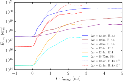
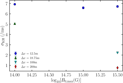
Extended Data Figure 1: (Top) Same as the inset in Fig. 1 in the main article, but with $\Delta x_{\rm finest}=18.75$ m for $B_{0,\mathrm{max}}=10^{14}$ G (cyan). The blue- and red-dotted curves show the evolution for $\Delta x_{\rm finest}=12.5$ m and $B_{0,\mathrm{max}}=10^{14}$ G magnified by a factor of $10^{3}$ and $10^{2}$, respectively.(Bottom) Dependence of the growth rate of the electromagnetic energy at the merger due to the Kelvin-Helmholtz instability on the initial magnetic field strength $B_{0,\mathrm{max}}$ and grid resolution. The error is due to the fitting.

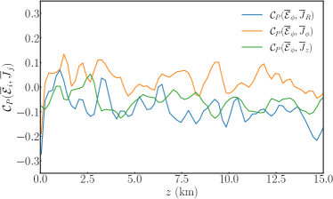
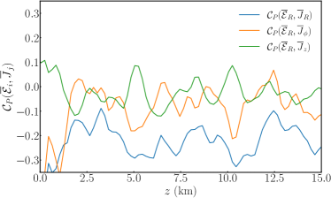
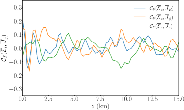
Extended Data Figure 2: Time-averaged correlations between the electromotive force and mean current components for $R=30$ km.

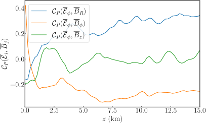
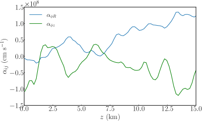
Extended Data Figure 3: (Left) Time-averaged correlations between the toroidal electromotive force and the magnetic field components for $R=30$ km. (Right) Alpha tensor components $\alpha_{\phi i}$ with $i\in[R,z]$ for $R=30$ km.

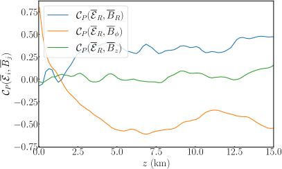
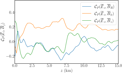
Extended Data Figure 4: Time-averaged correlations between the poloidal electromotive force and magnetic field components for $R=30$ km.

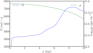
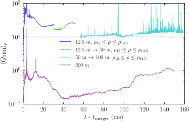
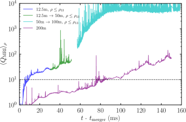
Extended Data Figure 5: (Top-left) The radial profile of the angular velocity (blue) and the rest-mass density (green) on the equatorial plane at $t-t_{\mathrm{merger}}\approx 50$ ms. Magnetorotational instability is inactive in a region with $x\lesssim 9$ km and $\rho\gtrsim 10^{14.5}~{}\rm{g/cm^{3}}$. (Top-right) Magnetorotational instability quality factor in a core region as a function of time. The remnant core is defined by a region with $\rho\geq 10^{13}~{}\rm{g/cm^{3}}$. The blue curve denotes the employed finest grid resolution of $12.5$ m. At $t-t_{\mathrm{merger}}\approx 30$ ms, the two finest domains with $\Delta x_{\rm finest}=12.5$ m and $\Delta x=25$ m are removed. Thus, the employed grid resolution is $\Delta x_{\rm finest}=50$ m plotted with the green curve. At $t-t_{\mathrm{merger}}\approx 50$ ms, the finest domain with $\Delta x_{\rm finest}=50$ m is removed and the subsequent evolution with $\Delta x_{\rm finest}=100$ m is plotted with the cyan curve. The result with $\Delta x_{\rm finest}=200$ m is plotted with the purple curve. (Bottom) The same as the middle panel, but for an envelope defined by a region with $10^{7}~{}{\rm g/cm^{3}}\leq\rho\leq 10^{13}~{}{\rm g/cm^{3}}$.

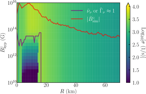
Extended Data Figure 6: Growth rate of the fastest growing mode of the neutrino viscous/drag magnetorotational instability as a function of the radius of the remnant massive neutron star and the hypothetical value of the $z$-component of the magnetic field $B^{z}_{\mathrm{hyp}}$. We take the simulation data on the orbital plane at $t-t_{\mathrm{merger}}\approx 10$ ms. The purple curve denotes the boundary where $\tilde{\nu}_{\nu}$ or $\tilde{\Gamma}_{\nu}\approx 1$. Outside the boundary, the growth rate is essentially the same as the ideal magnetorotational instability. The red curve denotes the $z$-component of the azimuthally averaged magnetic field strength in the simulation.

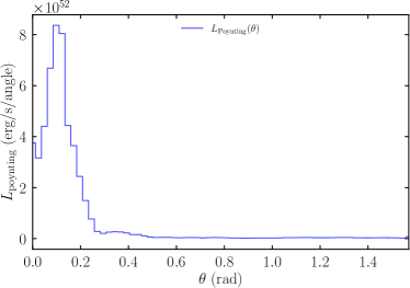
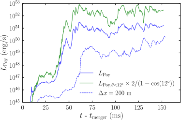
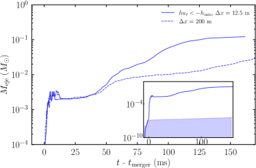
Extended Data Figure 7: (Top-left) Angular distribution of the luminosity of the Poyinting flux at the end of the simulation of $t-t_{\mathrm{merger}}\approx 150$ ms. (Top-right) Luminosity for the Poynting flux as a function of the post-merger time. The green curve is the jet-opening-angle corrected luminosity. The blue-dashed curve plots the luminosity for the simulation with $\Delta x_{\rm finest}=200$ m. (Bottom) Ejecta as a function of the post-merger time. The solid curve denotes the ejecta satisfying the Bernoulli criterion. The colored region in the inset shows the violation of the baryon mass conservation. The blue-dashed curve plots the luminosity for the simulation with $\Delta x_{\rm finest}=200$ m.

References

This work used computational resources of the supercomputer Sakura clusters at the Max Planck Computing and Data Facility. The simulation was also performed on Cobra, Raven at the Max Planck Computing and Data Facility, Fugaku provided by RIKEN through the HPCI System Research Project (Project ID: hp220174, hp230084), and the Cray XC50 at CfCA of the National Astronomical Observatory of Japan. This work was in part supported by the Grant-in-Aid for Scientific Research (grant Nos. 20H00158, 23H01172 and 23H04900) of Japan MEXT/JSPS. K.K. thanks to the Computational Relativistic Astrophysics members in AEI for a stimulating discussion. K.K. also thanks to Kota Hayashi and Koutarou Kyutoku for the helpful discussion and providing the initial data.

K.K. and A.R. were the primary drivers of the project and wrote the main text and method sections and developed the figures. M. S., Y. S., and K.K. are primarily developers of the numerical relativity code from scratch. K.K. performed the numerical relativity simulations. A. R. analyzed the simulation data. M. S. prepared an infrastructure of large-scale numerical computations. All authors were involved in interpreting the results and discussed the results, and commented on and/or edit the text.

The authors declare no competing financial interests.

Correspondence and requests for material should be addressed to K.K. (kenta.kiuchi@aei.mpg.de).

The data that support the findings of this study are available from the corresponding author upon reasonable request.

The numerical relativity code and data analysis tool are available from the correspond author upon reasonable request.

References

- [1] Abbott, B. P. et al., Multi-messenger Observations of a Binary Neutron Star Merger. Astrophys. J. Lett. 848, L12 (2017).
- [2] Goldstein, A. et al., An Ordinary Short Gamma-Ray Burst with Extraordinary Implications: Fermi-GBM Detection of GRB 170817A. Astrophys. J. Lett. 848, L14 (2017).
- [3] Savchenko, V. et al., INTEGRAL Detection of the First Prompt Gamma-Ray Signal Coincident with the Gravitational-wave Event GW170817. Astrophys. J. Lett. 848, L15 (2017).
- [4] Mooley, K. P. et al., Superluminal motion of a relativistic jet in the neutron-star merger GW170817. Nature 561, 355 (2018).
- [5] Mösta, P. et al., A magnetar engine for short GRBs and kilonovae. Astrophys. J. Lett. 901, L37 (2020).
- [6] Brandenburg, A., & Subramanian, K., Astrophysical magnetic fields and nonlinear dynamo theory. Phys. Rept. 417, 1 (2005).
- [7] Reboul-Salze, A., Guilet, J., Raynaud, R., & Bugli, M., MRI-driven dynamos in protoneutron stars. Astrophys. J. 667, A94 (2022).
- [8] Metzger, B. D. et al., The Proto-Magnetar Model for Gamma-Ray Bursts. Mon. Not. Roy. Astron. Soc. 413, 2031 (2011).
- [9] Abbott, B. P. et al., GW170817: Observation of Gravitational Waves from a Binary Neutron Star Inspiral. Phys. Rev. Lett. 119, 161101 (2017).
- [10] Metzger, B. D. et al., Electromagnetic counterparts of compact object mergers powered by the radioactive decay of r-process nuclei. Mon. Not. Roy. Astron. Soc. 406, 2650 (2010).
- [11] Lattimer, J. M., & Schramm, D. N., Black-Hole-Neutron-Star Collisions. Mon. Not. Roy. Astron. Soc. 192, L145 (1974).
- [12] Eichler, D., Livio,, M., Piran, T., & Schramm, D. N., Nucleosynthesis, neutrino bursts and -rays from coalescing neutron stars. Nature 340, 126 (1989).
- [13] Wanajo, S. et al., Production of all the -process nuclides in the dynamical ejecta of neutron star mergers. Astrophys. J. Lett. 789, L39 (2014).
- [14] Shibata, M. et al., Modeling GW170817 based on numerical relativity and its implications. Phys. Rev. D 96, 123012 (2017).
- [15] Kasen, D. et al., Origin of the heavy elements in binary neutron-star mergers from a gravitational wave event. Nature 551, 80 (2017).
- [16] Radice, D., Perego, A., Zappa, F., & Bernuzzi, S., GW170817: Joint Constraint on the Neutron Star Equation of State from Multimessenger Observations. Astrophys. J. Lett. 852, L29 (2018).
- [17] Metzger, B. D., Thompson, T. A., & Quataert, E., A magnetar origin for the kilonova ejecta in GW170817. Astrophys. J. 856, 101 (2018).
- [18] Fujibayashi, S., et al., Mass Ejection from the Remnant of a Binary Neutron Star Merger: Viscous-Radiation Hydrodynamics Study. Astrophys. J. 860, 64 (2018).
- [19] Perego, A., Radice, D., & Bernuzzi, S., AT 2017gfo: An Anisotropic and Three-component Kilonova Counterpart of GW170817. Astrophys. J. Lett. 850, L37 (2017).
- [20] Waxman, E., Ofek, E. O., Kushnir, D., & Avishay, G.-Y., Constraints on the ejecta of the GW170817 neutron-star merger from its electromagnetic emission. Mon. Not. Roy. Astron. Soc. 481, 3423 (2018).
- [21] Kawaguchi, K., Shibata, M., & Tanaka, M., Radiative transfer simulation for the optical and near-infrared electromagnetic counterparts to GW170817. Astrophys. J. Lett. 865, L21 (2018).
- [22] Breschi, M. et al., AT2017gfo: Bayesian inference and model selection of multicomponent kilonovae and constraints on the neutron star equation of state. Mon. Not. Roy. Astron. Soc. 505, 1661 (2021).
- [23] Nedora, V. et al., Numerical Relativity Simulations of the Neutron Star Merger GW170817: Long-Term Remnant Evolutions, Winds, Remnant Disks, and Nucleosynthesis. Astrophys. J. 906, 98 (2021).
- [24] Villar, V. A. et al., The Combined Ultraviolet, Optical, and Near-Infrared Light Curves of the Kilonova Associated with the Binary Neutron Star Merger GW170817: Unified Data Set, Analytic Models, and Physical Implications. Astrophys. J. Lett. 851, L21 (2017).
- [25] Ruiz, M., Shapiro, S. L., & Tsokaros, A., GW170817, General Relativistic Magnetohydrodynamic Simulations, and the Neutron Star Maximum Mass. Phys. Rev. D 97, 021501 (2018).
- [26] Fernández, R. et al., Long-term GRMHD simulations of neutron star merger accretion discs: implications for electromagnetic counterparts. Mon. Not. Roy. Astron. Soc. 482, 3373 (2019).
- [27] Shibata, M., Fujibayashi, S., & Sekiguchi, Y., Long-term evolution of a merger-remnant neutron star in general relativistic magnetohydrodynamics: Effect of magnetic winding. Phys. Rev. D 103, 043022 (2021).
- [28] Mösta, P. et al., A large scale dynamo and magnetoturbulence in rapidly rotating core-collapse supernovae. Nature 528, 376 (2015).
- [29] Kiuchi, K., Held, L. E., Sekiguchi, Y., & Shibata, M., Implementation of advanced Riemann solvers in a neutrino-radiation magnetohydrodynamics code in numerical relativity and its application to a binary neutron star merger. Phys. Rev. D 106, 124041 (2022).
- [30] Kiuchi, K., Kyutoku, K., Sekiguchi, Y., & Shibata, M., Global simulations of strongly magnetized remnant massive neutron stars formed in binary neutron star mergers. Phys. Rev. D 97, 124039 (2018).
- [31] Banik, S., Hempel, M., & Bandyopadhyay, D., New Hyperon Equations of State for Supernovae and Neutron Stars in Density-dependent Hadron Field Theory. Astrophys. J. Suppl. 214, 22 (2014).
- [32] Fujibayashi, S. et al., Postmerger Mass Ejection of Low-mass Binary Neutron Stars. Astrophys. J. 901, 122 (2020).
- [33] Kiuchi, K. et al., High resolution numerical-relativity simulations for the merger of binary magnetized neutron stars. Phys. Rev. D 90, 041502 (2014).
- [34] Lorimer, D. R., Binary and Millisecond Pulsars. Living Rev. Rel. 11, 8 (2008).
- [35] Kiuchi, K. et al., Efficient magnetic-field amplification due to the Kelvin-Helmholtz instability in binary neutron star mergers. Phys. Rev. D 92, 124034 (2015).
- [36] Price, D. J., & Rosswog, S., Producing Ultrastrong Magnetic Fields in Neutron Star Mergers. Science 312, 719 (2006).
- [37] Rasio, F. A., & Shapiro, S. L., TOPICAL REVIEW: Coalescing binary neutron stars. Classical and Quantum Gravity 16, R1 (1999).
- [38] Liu, Y. T., & Shapiro, S. L., Magnetic braking in differentially rotating, relativistic stars. Phys. Rev. D 69, 044009 (2004).
- [39] Balbus, S. A., & Hawley, J. F., A Powerful Local Shear Instability in Weakly Magnetized Disks. I. Linear Analysis. Astrophys. J. 376, 214 (1991).
- [40] Parker, E. A., Hydromagnetic Dynamo Models. Astrophys. J. 122, 293 (1955).
- [41] Yoshimura, H., Solar-cycle dynamo wave propagation. Astrophys. J. 201, 740 (1975).
- [42] Berger, E., Short-Duration Gamma-Ray Bursts. Ann. Rev. Astron. Astrophys. 52 43 (2014).
- [43] Sekiguchi, Y., Kiuchi, K., Kyutoku, K., & Shibata, M., Dynamical mass ejection from binary neutron star mergers: Radiation-hydrodynamics study in general relativity. Phys. Rev. D 91, 064059 (2015).
- [44] Blandford, R. D., & Payne, D. G., Hydromagnetic flows from accretion discs and the production of radio jets. Mon. Not. Roy. Astron. Soc. 199, 883 (1982).
- [45] Tanaka, M., & Hotokezaka, K., Radiative Transfer Simulations of Neutron Star Merger Ejecta. Astrophys. J. 775, 113 (2013).
- [46] Fujibayashi, S. et al., Mass ejection from disks surrounding a low-mass black hole: Viscous neutrino-radiation hydrodynamics simulation in full general relativity. Phys. Rev. D 101, 083029 (2020).
- [47] Metzger, B. D., Piro, A. L., & Quataert, E., Neutron-Rich Freeze-Out in Viscously Spreading Accretion Disks Formed from Compact Object Mergers. Mon. Not. Roy. Astron. Soc. 396, 304 (2009).
- [48] Hayashi, K. et al., Properties of the remnant disk and the dynamical ejecta produced in low-mass black hole-neutron star mergers. Phys. Rev. D 103, 043007 (2021).
- [49] Salvesen, G., Simon, J. B., Armitage, P. J., & Mitchell, C., Accretion disc dynamo activity in local simulations spanning weak-to-strong net vertical magnetic flux regimes. Mon. Not. Roy. Astron. Soc. 457, 857 (2016).
- [50] Shibata, M. & Namamura, T., Evolution of three-dimensional gravitational waves: Harmonic slicing case. Phys. Rev. D 52, 5428-5444 (1995).
- [51] Baumgarte, T. W. & Shapiro, S. L., On the numerical integration of Einstein’s field equations. Phys. Rev. D 59, 024007 (1998).
- [52] Baker, J. G. et al., Gravitational wave extraction from an inspiraling configuration of merging black holes. Phys. Rev. Lett. 96, 111102 (2006).
- [53] Campanelli, M., Lousto, C. O., Marronetti, P., & Zlochower, Y., Accurate evolutions of orbiting black-hole binaries without excision. Phys. Rev. Lett. 96, 111101 (2006).
- [54] Hilditch, D. et. al, Compact binary evolutions with the Z4c formulation. Phys. Rev. D 88, 084057 (2013).
- [55] Mignone, A., Ugliano, M., & Bodo, G., A five-wave HLL Riemann solver for relativistic MHD. Mon. Not. Roy. Astron. Soc. 393, 1141 (2009).
- [56] Gardiner, T. A., & Stone, J. M., An Unsplit Godunov Method for Ideal MHD via Constrained Transport in Three Dimensions. J. Comput. Phys. 227, 4123-4141 (2008).
- [57] Sekiguchi, Y., Kiuchi, K., Kyutoku, K., & Shibata, M., Current Status of Numerical-Relativity Simulations in Kyoto. PTEP 2012, 01A304 (2012).
- [58] http://www.lorene.obspm.fr/
- [59] Timmes, F. X., & Swesty, F. D., The Accuracy, Consistency, and Speed of an Electron-Positron Equation of State Based on Table Interpolation of the Helmholtz Free Energy. Astrophys. J. Suppl. 126, 501 (2000).
- [60] Kiuchi, K., Kyutoku, K., Sekiguchi, Y., & Shibata, M., Global simulations of strongly magnetized remnant massive neutron stars formed in binary neutron star mergers. Phys. Rev. D 97, 124039 (2018).
- [61] Viganò, D. et al., General relativistic MHD large eddy simulations with gradient subgrid-scale model. Phys. Rev. D 101, 123019 (2020).
- [62] Chandrasekhar, S., HYDRODYNAMIC AND HYDROMAGNETIC STABILITY. Oxford: Clarendon (1961).
- [63] Racine, É. et al., On the Mode of Dynamo Action in a Global Large-eddy Simulation of Solar Convection. Astrophys. J. 735, 46 (2011).
- [64] Balbus, S. A., & Hawley, J. F., A Powerful Local Shear Instability in Weakly Magnetized Disks. I. Linear Analysis. Astrophys. J. 376, 214 (1991).
- [65] Guilet, J., Bauswein, A., Just, O., & Janka, H. T., Magnetorotational instability in neutron star mergers: impact of neutrinos. Mon. Not. Roy. Astron. Soc. 471, 1879 (2016).
- [66] Meier, D. L., A Magnetically Switched, Rotating Black Hole Model for the Production of Extragalactic Radio Jets and the Fanaroff and Riley Class Division. Astrophys. J. 522, 753 (1999).
- [67] Shibata, M., Suwa, Y., Kiuchi, K, & Ioka, K., Afterglow of a Binary Neutron Star Merger. Astrophys. J. Lett. 734, L36 (2011).
- [68] Kiuchi, K., Kyutoku, K., & Shibata, M., Three dimensional evolution of differentially rotating magnetized neutron stars. Phys. Rev. D 86 064008 (2012).