Refractive neutrino masses, ultralight dark matter and cosmology

Abstract

We consider in detail a possibility that the observed neutrino oscillations are due to refraction on ultralight scalar boson dark matter. We introduce the refractive mass squared, $\tilde{m}^{2}$, and study its properties: dependence on neutrino energy, state of the background, etc. If the background is in a state of cold gas of particles, $\tilde{m}^{2}$ shows a resonance dependence on energy. Above the resonance ($E\gg E_{R}$), we find that $\tilde{m}^{2}$ has the same properties as usual vacuum mass squared. Below the resonance, $\tilde{m}^{2}$ decreases with energy, which (if realised) allows us to avoid the cosmological bound on the sum of neutrino masses. Also, $\tilde{m}^{2}$ may depend on time. We consider the validity of the results: effects of multiple interactions with scalars, and modification of the dispersion relation. We show that for values of parameters of the system required to reproduce the observed neutrino masses, perturbativity is broken at low energies, which border above the resonance. If the background is in the state of coherent classical field, the refractive mass does not depend on energy explicitly but may show time dependence. It coincides with the refractive mass in a cold gas at high energies. Refractive nature of neutrino mass can be tested by searches of its dependence on energy and time.

I Introduction

One of the greatest achievements in particle physics is “… the discovery of neutrino oscillations, which shows that neutrinos have mass”. Indeed, oscillations of atmospheric neutrinos Kajita:2016cak and adiabatic conversion of solar neutrinos McDonald:2016ixn have been discovered. But how do we know that the neutrino mass is behind the oscillations and conversion? Smallness of the observed neutrino mass and large mixing may testify that its nature differs from nature of other fermions.

In 1978, Wolfenstein proposed the oscillations of massless neutrinos Wolfenstein:1977ue . For this, he introduced point-like four-fermion interactions (what we call now NSI) which generate effective potentials experienced by neutrinos. The potentials mix neutrinos and give splitting of energy eigenvalues of propagation. Presumably, the interactions are due to exchange of heavy mediators. Therefore the potentials, and consequently, oscillation effects do not depend on neutrino energy.

However, the energy dependence of oscillations was found in experiments! Furthermore, the dependence is in agreement with the presence of the mass term in the Hamiltonian of evolution:

$$H\sim\sqrt{p^{2}+|m|^{2}}\approx p+\frac{|m|^{2}}{2E}\,,$$

(in 3 $\nu$ case $m^{2}\rightarrow MM^{\dagger}$, where $M$ is $3\times 3$ mass matrix). It is this energy dependence of the oscillation effects which provides a convincing argument that the neutrino mass is behind oscillations.

Still, this is not the end of the story. Notice that oscillations of relativistic neutrinos probe mass-squared and not the mass. Furthermore,

(i) mass changes the chirality of fermions, while the mass-squared does not.

(ii) The mass operator of neutrinos has a gauge charge and appears as a result of symmetry breaking. In contrast, modulus of mass squared is gauge invariant and does not require symmetry breaking. Therefore, in oscillations there is no direct probe of mass, and any contribution to the Hamiltonian of evolution which has an $A/E$ form with a constant $A$ can reproduce the oscillation data.

In fact, at high enough energies the potential generically has a $1/E$ dependence. In the Standard Model (SM), the potentials have the $1/E$ dependence above the threshold of production of the $W-$ and $Z-$ boson mediators, i.e., for $s\gtrsim m_{\rm mediator}^{2}$ Lunardini:2000swa . For neutrino scattering on electrons due to $W-$boson exchange, this requires the neutrino energy in the laboratory frame $E\gtrsim m_{W}^{2}/2m_{e}=6\cdot 10^{6}$ GeV. If mediator is light, the $1/E$ dependence of the potential shows up at low observable energies. This opens up a possibility to substitute, to some extent, the vacuum mass term in the Hamiltonian by the energy-dependent potential Choi:2019zxy ; Ge:2020ffj; Ge:2020xkm; Choi:2020ydp ; Chun:2021ief .

Since oscillations are observed in “vacuum”, where interactions with matter can be neglected, the scatterers should be new light particles that fill the space, thus being a component of the Dark Matter (DM). For example, fuzzy DM fits all these requirements Hu:2000ke ; Hui:2016ltb . In this connection, refraction effects of neutrinos on very light target particles due to exchange of light mediators were studied and the effective potentials were computed Choi:2019zxy ; Choi:2020ydp ; Smirnov:2021zgn . The phenomenology of neutrino-ultralight DM interactions has been explored extensively Berlin:2016woy ; Krnjaic:2017zlz ; Brdar:2017kbt ; Capozzi:2018bps ; Dev:2020kgz ; Losada:2021bxx ; Huang:2021kam ; Chun:2021ief ; Dev:2022bae ; Huang:2022wmz ; Davoudiasl:2023uiq ; Losada:2023zap ; Gherghetta:2023myo .

In this paper we address the following questions: can the potential with $1/E$ dependence substitute the mass completely? Can one distinguish the usual mass and potential in oscillations or in some other way ?

One fundamental difference exists between neutrino mass generation by vacuum expectation value (VEV) and that by refraction. Refractive mass is proportional to the number density of DM particles: $m^{2}\propto n$, and therefore the neutrino mass would increase in the past with redshift as $(z+1)^{3/2}$. If the present ($z=0$) neutrino mass bound is considered for the heaviest active neutrino, then in the epoch of photon decoupling $(z\sim 1000)$, the neutrino mass would become $O(10)$ eV (see details in the text). This violates the cosmological bound on the sum of neutrino masses from observations of the cosmic microwave background (CMB), as well as bounds from structure formation Planck:2018vyg . The cosmological bound still allows contribution to the neutrino mass at the level $3\cdot 10^{-3}\,{\rm eV}$, affecting solar neutrinos Berlin:2016woy .

In this paper, we consider a realistic scenario of the refractive mass with three active neutrinos which can reproduce all the oscillation data. We further elaborate on the properties of refractive neutrino masses. It will be shown that by appropriate selection of the resonance energy, the cosmological bound may be satisfied. Dependence of the refractive masses on he state of medium is discussed. We also study perturbativity violation due to multiple interactions of neutrino with the dark matter particles.

The paper is organized as follows. In sect. II, we introduce the refractive neutrino mass in a cold bath of scalar particles and study its properties. We show that with appropriate choice of parameters the existing experimental data on neutrino oscillations can be explained. In sect. III, the conditions of perturbativity violation and validity of the results are considered. In sect. IV, we discuss the refraction of neutrinos in a classical field that describes a coherent state of scalar particles, and the corresponding contribution to the neutrino mass matrix. We discuss constraints arising from astrophysical sources, terrestrial laboratories as well as the early Universe in sect. V and determine the viable parameter space. Finally, we summarize our results and conclude in sect. VI.

II Refractive masses of neutrinos in cold particle bath.

II.1 Effective potential and refractive mass

Let us consider the propagation of massless neutrinos $(\nu_{e},\nu_{\mu},\nu_{\tau})$ in a medium composed of ultralight scalar bosons $\phi$ and their antiparticles $\bar{\phi}$ with number densities $n_{\phi}$ and $\bar{n}_{\phi}$ correspondingly. These ultralight scalars can act as the cold DM, or compose a part of the DM. Neutrinos scatter on the scalars via exchange of light fermionic mediators $\chi_{k}$ due to the Yukawa couplings,

$$\mathcal{L}\supset\sum_{\alpha=e,\mu,\tau}\sum_{k}g_{\alpha k}\bar{\chi}_{kR}\nu_{\alpha L}\phi^{*}+m_{\chi k}\bar{\chi}_{kR}\chi_{kL}+{\rm h.c}\,.$$ (1)

There are two possible cases: Dirac fermion mediators and Majorana mediators: in the latter case $\chi_{kL}\rightarrow(\chi_{kR})^{c}$. As we will see, in order to explain the oscillation data, at least two mediators are needed with different couplings $g_{\alpha k}$.

The elastic forward scattering $\nu\phi\rightarrow\nu\phi$ in the cold gas of $\phi-$particles produces the effective potential through the $s-$channel and $u-$channel scattering as shown in Fig. 1  Choi:2019zxy ; Choi:2020ydp ; Smirnov:2021zgn ,

$$V_{\alpha\beta}=\sum_{k}g_{\alpha k}g_{\beta k}^{*}\,\left[\frac{\bar{n}_{\phi}(2Em_{\phi}-m_{\chi k}^{2})}{(2Em_{\phi}-m_{\chi k}^{2})^{2}+(m_{\chi}\Gamma_{\chi k})^{2}}+\frac{n_{\phi}}{2Em_{\phi}+m_{\chi k}^{2}}\right]\,,$$ (2)

where $E$ is the neutrino energy, $m_{\phi}$ is the mass of $\phi$, and $\Gamma_{\chi k}\equiv\sum_{\alpha}g_{\alpha k}^{2}m_{\chi k}/(8\pi)$ is the total decay rate of the mediator $\chi_{k}$. We consider non-relativistic $\phi$ and neglect its mass-squared in the denominator in (2).

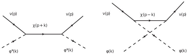
Figure 1: Feynman diagrams for scattering of neutrinos on the $\phi$ background. Left: $s-$channel. Right: $u-$channel.

The first term in (2) corresponds to $\chi_{k}$ exchange in the $s-$channel and for $m_{\chi k}>m_{\phi}$ it has a resonance character. For simplicity, we will introduce two mediators with nearly the same masses: $m_{\chi k}\approx m_{\chi}$. According to (2), for $\phi$ at rest, the resonance energy equals

$$E_{R}\simeq\frac{m_{\chi}^{2}}{2m_{\phi}}.$$ (3)

The second term in (2) is due to $\chi_{k}$ exchange in the $u-$channel. For antineutrinos, the potential can be obtained from (2) by interchanging $n_{\phi}\leftrightarrow\bar{n}_{\phi}$.

In the $\phi-$background, the Hamiltonian of evolution of massless neutrinos $(\nu_{e},\nu_{\mu},\nu_{\tau})$ is given by

$$H\simeq{V},$$ (4)

where ${V}=||V_{\alpha\beta}||$ is the matrix of potentials. We introduce the refractive neutrino mass squared as

$$\tilde{m}_{\alpha\beta}^{2}\equiv 2EV_{\alpha\beta}\,,$$

or, in a matrix form as

$$\tilde{m}^{2}=2EV.$$ (5)

Then the Hamiltonian can be written in the form of the vacuum term:

$$H\simeq\frac{\tilde{m}^{2}}{2E}\,.$$ (6)

Let us study the properties of the refractive masses-squared $\tilde{m}_{\alpha\beta}^{2}$. In terms of the dimensionless parameter $y\equiv E/E_{R}$, the refractive mass (5), with $V$ given in (2), can be written as

$$\tilde{m}_{\alpha\beta}^{2}=2yE_{R}\sum_{k}V_{\alpha\beta k}^{0}\,\left[\frac{(1-\epsilon)(y-1)}{(y-1)^{2}+\tilde{\xi}_{k}^{2}}+\frac{1+\epsilon}{1+y}\right]\,.$$ (7)

Here

$$V_{\alpha\beta k}^{0}\equiv\frac{g_{\alpha k}g_{\beta k}^{*}}{2m_{\chi}^{2}}(n_{\phi}+\bar{n}_{\phi}),$$ (8)

$\epsilon$ is the C-asymmetry of background:

$$\epsilon\equiv\frac{n_{\phi}-\bar{n}_{\phi}}{n_{\phi}+\bar{n}_{\phi}}\,,~{}~{}~{}(\epsilon=-1\div 1),$$ (9)

and $\tilde{\xi}_{k}\equiv\Gamma_{\chi k}/m_{\chi}$. Since the couplings are very small, we have $\tilde{\xi}_{k}\ll 1$, and therefore $\tilde{\xi}_{k}$ can be neglected everywhere apart from a very narrow region around the resonance, $y=1$. The energy dependent factor in the brackets of (7) does not depend on mediator type $k$ and becomes universal for all the contributions. Then using explicit expressions for $V_{\alpha\beta k}^{0}$ and $E_{R}$, the matrix of refractive mass-squared can be written as

$$\tilde{m}^{2}=\lambda\frac{n_{\phi}+\bar{n}_{\phi}}{m_{\phi}}~{}\frac{y(y-\epsilon)}{y^{2}-1}\,,$$ (10)

where $\lambda$ is the matrix of couplings:

$$\lambda=||\lambda_{\alpha\beta}||,~{}~{}~{}~{}~{}\lambda_{\alpha\beta}=\sum_{k}g_{\alpha k}g_{\beta k}^{*}\,.$$

Introducing vectors of Yukawa couplings $\vec{g}^{T}_{k}\equiv(g_{ek},g_{\mu k},g_{\tau k})$, $\lambda$ can be expressed as

$$\lambda=\sum_{k}\vec{g}^{T}_{k}\times\vec{g}_{k}\,.$$ (11)

Notice that $\tilde{m}^{2}$ in (10) does not depend on the mediator mass explicitly. Defining

$$\tilde{m}^{2}_{\rm asy}\equiv\lambda\frac{n_{\phi}+\bar{n}_{\phi}}{m_{\phi}},$$ (12)

the effective mass-squared (10) becomes

$$\tilde{m}^{2}=\tilde{m}^{2}_{\rm asy}\frac{y(y-\epsilon)}{y^{2}-1}\,.$$ (13)

Since the contribution of $\phi$ to the energy density of the Universe

$$\rho_{\phi}=m_{\phi}(n_{\phi}+\bar{n}_{\phi})\,,$$ (14)

we can rewrite the refractive masses (12) as

$$\tilde{m}^{2}_{\rm asy}=\lambda\frac{\rho_{\phi}}{m_{\phi}^{2}}\,.$$ (15)

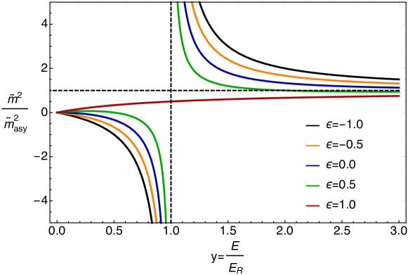
Figure 2: The rescaled refractive mass squared $\tilde{m}^{2}/\tilde{m}^{2}_{\rm asy}$ as function of rescaled energy, $y$, for different values of the asymmetry $\epsilon$.

The dependence of (13) is shown in Fig. 2 and Fig. 3. In Fig. 2, we present the ratio $\tilde{m}^{2}/\tilde{m}^{2}_{\rm asy}$ as a function of the rescaled energy $y$ for different values of the asymmetry $\epsilon$. Fig. 3 shows the dependence of the absolute values of the refractive mass squared $|\tilde{m}^{2}|$ on $y$. The mass squared has the following properties:

1. For very low energies, $y\ll 1$, we have

   $$\tilde{m}^{2}/\tilde{m}^{2}_{\rm asy}=y(\epsilon-y).$$ (16)

   When $y\rightarrow 0$, it decreases as $y\epsilon$. For $\epsilon=1$, the potential reproduces the Wolfenstein potential $V=2V_{0}=(g^{2}/m_{\chi}^{2})n_{\phi}$. In the C-symmetric medium, $\epsilon=0$, the mass squared has an additional suppression factor $y$:

   $$\tilde{m}^{2}/\tilde{m}^{2}_{\rm asy}=-y^{2}.$$

2. At resonance, $y=1$, the contribution from the $s-$channel diagram is zero, and it changes sign as the energy falls below the resonance energy. The contribution from the $u-$channel slightly shifts the pole to $\tilde{m}^{2}=\tilde{m}^{2}_{\rm asy}(1+\epsilon)/2$.

3. In the limit of high energies, $y\gg(1,\epsilon)$, with increase of $y$, the mass converges to the asymptotic value: $\tilde{m}^{2}\rightarrow\tilde{m}^{2}_{\rm asy}$. According to (13), the masses reduce to

   $$\tilde{m}^{2}/\tilde{m}^{2}_{\rm asy}=\left\{\begin{matrix}1-\frac{\epsilon}{y}~{},~{}~{}~{}~{}~{}\epsilon\neq 0\,.\\ 1+y^{-2}~{},~{}~{}~{}\epsilon=0\,.\end{matrix}\right.$$ (17)

   The convergence is faster for zero asymmetry.

4. For antineutrinos, the refractive mass squared can be obtained by changing the sign of C-asymmetry: $\epsilon\rightarrow-\epsilon$. While at low energies, this changes the sign of $\tilde{m}_{\alpha\beta}^{2}$, at high energies, $y\gg 1$, the mass $\tilde{m}_{\alpha\beta}^{2}$ is nearly the same for neutrinos and antineutrinos. This contradicts the statement in Ge:2019tdi .

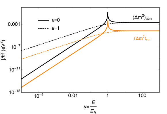
Figure 3: The moduli of eigenvalues of the refractive mass-squared matrix, $|\tilde{m}^{2}|$, as a function of rescaled energy. In asymptotics, $y\gg 1$, they can reproduce the solar and the atmospheric neutrino mass-squared differences.

Thus, at high energies, $E\gg E_{R}$, the refractive mass-squared $\tilde{m}^{2}$ has the same properties as the usual vacuum mass-squared $m^{2}$: no dependence on energy, the same for neutrinos and antineutrinos. This is not surprising: essentially, in this case, the VEV (classical scalar field at the lowest energy state) is substituted by scalar particles – quanta of the scalar field. Furthermore, at high enough density (occupation number), the sea of scalar particles can be treated as a classical scalar field, as we will discuss later.

Similarly, due to interaction with $\phi$ and $\nu$, the fermion $\chi$ acquires a refraction mass $\tilde{m}_{\chi k}^{2}$ which is of the same order as the neutrino refraction mass.

II.2 Refractive mass and the neutrino oscillation data

For a single mediator, the matrix of couplings $\lambda=\vec{g}^{T}\times\vec{g}$ has rank 1, that is, in the $3\nu-$case, only one neutrino gets an effective mass and only two mixings are defined. Therefore, the second mediator should be introduced with different set of couplings to active neutrinos. In this case, 6 real couplings can explain 6 real parameters: three mass squared differences and three mixing angles. For complex coupling constants, the CP-violation phase can be obtained. Moreover, 5 couplings are enough, so that one of the couplings can be set to zero to reproduce two $\Delta m^{2}$ and three angles.

Let us fix values of the parameters $g_{\alpha k}$, $m_{\phi}$ and $m_{\chi}$ to fit the neutrino oscillation data with refraction mass squared (7). For this, we consider the matrix of active neutrinos $\tilde{m}^{2}_{\alpha\beta}$ of the nearly tribimaximal (TBM) form Harrison:2002er . For

$$g_{e1}=g_{\mu 1}=g_{\tau 1}=g_{1},~{}~{}\,\,\,g_{e2}=0,\,\,~{}~{}g_{\mu 2}=-g_{\tau 2}=g_{2}\,,$$ (18)

the elements of the $3\times 3$ matrix $\tilde{m}^{2}_{\alpha\beta}$ become

$$\tilde{m}^{2}_{e\alpha}=g_{1}^{2}\,\frac{\rho_{\phi}}{m_{\phi}^{2}}\,,~{}~{}~{}~{}\alpha=e,\mu,\tau,$$ (19)

$$\tilde{m}^{2}_{\mu\mu}=\tilde{m}^{2}_{\tau\tau}=(g_{1}^{2}+g_{2}^{2})\frac{\rho_{\phi}}{m_{\phi}^{2}},~{}~{}~{}~{}\tilde{m}^{2}_{\mu\tau}=\tilde{m}^{2}_{\tau\mu}=(g_{1}^{2}-g_{2}^{2})\frac{\rho_{\phi}}{m_{\phi}^{2}}\,.$$ (20)

This exactly reproduces the TBM structure. Since the lightest neutrino mass is zero, the values of the parameters can be connected to the observed mass-squared differences as

$$g_{1}^{2}\frac{\rho_{\phi}}{m_{\phi}^{2}}=\frac{1}{3}\Delta m_{\rm sol}^{2}\,,~{}~{}~{}~{}g_{2}^{2}\frac{\rho_{\phi}}{m_{\phi}^{2}}=\frac{1}{2}\Delta m_{\rm atm}^{2}.$$ (21)

For normal mass ordering, we have from (21),

$$g_{1} = m_{\phi}\sqrt{\frac{\Delta m_{\rm sol}^{2}}{3\rho_{\phi}}}=3.2\cdot 10^{-10}\left(\frac{m_{\phi}}{10^{-10}\,{\rm eV}}\right)\,\left(\frac{\Delta m_{\rm sol}^{2}}{7.5\cdot 10^{-5}\,{\rm eV}^{2}}\right)^{1/2}\,\left(\frac{\rho_{\odot}}{\rho_{\phi}}\right)^{1/2}\,,$$

$$g_{2} = m_{\phi}\sqrt{\frac{\Delta m_{\rm atm}^{2}}{2\rho_{\phi}}}=2.2\cdot 10^{-9}\left(\frac{m_{\phi}}{10^{-10}\,{\rm eV}}\right)\,\left(\frac{\Delta m_{\rm atm}^{2}}{2.3\cdot 10^{-3}\,{\rm eV}^{2}}\right)^{1/2}\,\left(\frac{\rho_{\odot}}{\rho_{\phi}}\right)^{1/2}\,.$$ (22)

For numerical estimation, we assumed that $\phi$ compose the entire local DM energy density $\rho_{\odot}$, therefore, $\rho_{\phi}=\rho_{\odot}=0.3\,{\rm GeVcm}^{-3}$. The dependences (22) are shown in Fig. 7 together with various bounds, which we will discuss later. The relations (22) are based on asymptotic values of the effective masses and, therefore, practically do not depend on $m_{\chi}$.

The bounds on neutrino-scalar interactions coupling $g$ follow from laboratory experiments. Invisible decay of the Higgs ATLAS:2016neq , invisible Z-decay Electroweak:2003ram , meson decays Pasquini:2015fjv , and tau decays Brdar:2020nbj give bounds which are weaker than $g\sim 10^{-5}$. They are superseded by astrophysical and cosmological bounds. The strongest bound follows from cooling of stars: $g_{i}<10^{-7}$ Farzan:2018gtr ; Dev:2020eam . Therefore according to (22), we obtain an upper bound on the mass of scalar

$$m_{\phi}<5\cdot 10^{-9}\,{\rm eV}\left(\frac{g_{2}}{10^{-7}}\right)\,.$$ (23)

The upper bound on the resonance energy follows from non-observation of energy dependence of oscillation parameters, namely, increase of the effective mass squared with decrease of energy (see Fig. 2). The lowest energies of detected neutrinos are about 0.2 MeV (the solar pp-neutrinos). At these energies, oscillations are averaged and therefore are insensitive to $\Delta m^{2}$. The sensitivity appears in reactor neutrinos with $E\sim$ MeV. The accuracy of determination of $\Delta m^{2}$ is about $10\%$ and data are in agreement with constant $\Delta m^{2}$. Also no dependence on energy has been found in a wide energy range (from IC-Deep Core down to reactor neutrinos) and all the extractions of $\Delta m_{\rm atm}^{2}$ are in agreement within $10\%$. Therefore, according to (17), $y^{2}>10$ for $\epsilon=0$, and $y>10$ for $|\epsilon|=1$ are required. Taking the lowest testable energy 1 MeV, we find the upper bound on resonance energy $E_{R}<0.1$ MeV.

Figure 4: The allowed region in the $m_{\chi}-m_{\phi}$ plane. The pink shaded region corresponds to $E_{R}>0.1\,{\rm MeV}$ and is excluded by oscillation data. In the blue shaded region, $E_{R}<28\,{\rm eV}$ and this is excluded by cosmological considerations (see discussion in sect. V.1). The gray shaded region corresponds to $m_{\phi}>m_{\chi}$, thereby making the DM unstable. The hatched region is excluded by $\nu-\chi$ oscillations of solar neutrinos (see sect. IV.5).

The mass of mediator is determined by $m_{\phi}$ and resonance energy (3) through

$$m_{\chi}=\sqrt{2m_{\phi}E_{R}}\,.$$ (24)

From this equation and (23), we find

$$m_{\chi}<0.03\,{\rm eV}\,\left(\frac{m_{\phi}}{5\cdot 10^{-9}\,{\rm eV}}\right)^{1/2}\left(\frac{E_{R}}{0.1\,{\rm MeV}}\right)^{1/2}\,.$$ (25)

Fig. 4 shows $m_{\chi}$ as function of $m_{\phi}$ for different values of $E_{R}$.

III Scales and validity of results

For small enough $g/m_{\phi}$, and consequently small $\Delta m^{2}$, the results described above clearly work. However, with increase of $g/m_{\phi}$, various problems arise and the question we address in this section is whether we can still reproduce the observed values of the masses and avoid these problems.

III.1 Scales in the problem

Values of $m_{\phi}$, $m_{\chi}$ and minimal $E_{R}$ estimated in sect. II.2 determine several spatial scales, and consequently, the physical picture of the effects. The Compton length of the scalar has a macroscopic size:

$$\lambda_{c}=\frac{2\pi}{m_{\phi}}>2.5\cdot 10^{5}\,{\rm cm}\left(\frac{5\cdot 10^{-10}\,{\rm eV}}{m_{\phi}}\right)\,.$$

The number density of scalars equals

$$n_{\phi}=\frac{\rho_{\phi}}{m_{\phi}}>6\cdot 10^{17}\,{\rm cm}^{-3}\left(\frac{5\cdot 10^{-10}\,{\rm eV}}{m_{\phi}}\right)\,,$$

so that the distance between them

$$d\simeq n^{-1/3}\leq 1.2\cdot 10^{-6}\,{\rm cm}\,\left(\frac{m_{\phi}}{5\cdot 10^{-10}\,{\rm eV}}\right)^{1/3}\,.$$

In the Galaxy, the virialized velocity of DM is $v_{\rm vir}\sim 10^{-3}$, consequently, the de Broglie wavelength equals

$$\lambda_{dB}=\frac{2\pi}{m_{\phi}v_{\rm vir}}>2.5\cdot 10^{8}\,{\rm cm}\,\left(\frac{5\cdot 10^{-10}\,{\rm eV}}{m_{\phi}}\right).$$

Thus, the de Broglie length is bigger than typical baseline of laboratory experiments which means that production and detection of neutrinos occurs within a single de Broglie wavelength of the $\phi$. The radius of interaction is given by $m_{\chi}$:

$$r_{\chi}=\frac{1}{m_{\chi}}=6\cdot 10^{-4}~{}{\rm cm}\left(\frac{0.03~{}{\rm eV}}{m_{\chi}}\right)$$

below resonance and

$$r_{\chi}\simeq(2Em_{\phi})^{-1/2}$$

above resonance. Thus, we have

$$\lambda_{dB}\gg r_{\chi}\gg d\gg\lambda_{\nu},$$ (26)

where $\lambda_{\nu}$ is the wavelength of laboratory neutrinos. In the following sections, we will discuss the consequences of the hierarchy in scales and how this can change the results of the computations (2), which correspond to the standard $S$-matrix scattering formalism.

III.2 Wavefunction renormalization and Perturbativity

In the computation of (2), the propagator of the mediator $\chi$ equals

$$\mathrm{i}\frac{\not{p}_{\chi}+m_{\chi}}{p_{\chi}^{2}-m_{\chi}^{2}}=\mathrm{i}\frac{\not{p}\pm\not{k}+m_{\chi}}{p_{\chi}^{2}-m_{\chi}^{2}}\,,$$ (27)

where the signs $+$ and $-$ are for the $s-$ and $u-$ channels correspondingly. The potential (2) is produced by the term $\not{k}$, which gives $m_{\phi}\gamma_{0}$ in the non-relativistic case. The contribution $\not{p}$ is usually considered as the wavefunction (WF) renormalization. It modifies the potential in the next order of perturbation theory Choi:2019ixb . Notice, however, that the renormalization being proportional to $g_{\alpha k}g_{\beta k}^{*}$, is different for different neutrino species and therefore contributes to oscillations. It can be important when perturbation theory starts to break down.

Let us consider this in some detail. It is simpler to use the diagonalized (effective mass-squared) basis. The equation of motion for $i-$th neutrino component can be parameterized as

$$\left(\not{p}+\not{p}\Sigma_{1}^{i}+\not{k}\Sigma_{2}^{i}\right)u_{Li}=0\,,$$ (28)

where $\Sigma_{1,2}^{i}$ are the results of computation of the scattering amplitude. Here we assume that $\langle\phi\rangle=0$, so that any extra contribution to the equation of motion from the interaction terms in (1) is absent. From this equation, we obtain

$$\not{p}\,u_{Li}=-\frac{\not{k}\Sigma_{2}^{i}}{1+\Sigma_{1}^{i}}\,u_{Li}\,.$$ (29)

The amplitude of forward scattering is given by

$$A_{i}=\bar{u}_{Li}\left(\not{p}\Sigma_{1}^{i}+\not{k}\Sigma_{2}^{i}\right)u_{Li}\,.$$ (30)

Inserting here the expression for $\not{p}u_{Li}$ from (29), we obtain

$$A_{i}=\bar{u}_{Li}\not{k}u_{Li}\Sigma_{2}^{i}\left(1-\frac{\Sigma_{1}^{i}}{1+\Sigma_{1}^{i}}\right)\,.$$ (31)

For non-relativistic $\phi$, $\not{k}\approx m_{\phi}\gamma^{0}$. Eq. (31) gives the potential with the correction due to $\not{p}$ term included,

$$\tilde{V}^{i}=\frac{V^{i}}{1+\Sigma_{1}^{i}}\,.$$ (32)

The factor $1/{(1+\Sigma_{1}^{i}})$ is nothing but the effect of the WF renormalization. It is the next order correction in $g^{2}$ to $V$. In the perturbative regime, $\Sigma_{1}^{i}\ll 1$ and $\tilde{V}^{i}\approx V^{i}$.

Each of the factors $\Sigma_{1,2}^{i}$ has contributions from the $s-$ and $u-$ channel:

$$\Sigma_{1}^{i}=\Sigma_{1s}^{i}+\Sigma_{1u}^{i},\,\,\,\Sigma_{2}^{i}=\Sigma_{2s}^{i}+\Sigma_{2u}^{i}\,.$$

Furthermore, as can be seen from the expression for the propagator (27), the relations

$$\Sigma_{1s}^{i}=\Sigma_{2s}^{i},\,\,\,\Sigma_{1u}^{i}=-\Sigma_{2u}^{i}\,,$$ (33)

exist. In the lowest order, the potential equals

$$V^{i}=m_{\phi}(\Sigma_{2s}^{i}+\Sigma_{2u}^{i})\,.$$ (34)

Let us consider the correction due to WF renormalization for some specific cases:

1. For $\epsilon=-1$ (resonance $s-$contribution only), we have $\Sigma_{1u}^{i}=\Sigma_{2u}^{i}=0$, and from (33, 34), the perturbativity condition $\Sigma_{1}^{i}=\Sigma_{2}^{i}=V^{i}/m_{\phi}$. Therefore,

   $$\tilde{V}^{i}=\frac{V^{i}m_{\phi}}{m_{\phi}+V^{i}}\,.$$

   Consequently,

   $$\tilde{V}=\left\{\begin{matrix}V,~{}~{}m_{\phi}\gg V\,\,,\\ m_{\phi},~{}~{}m_{\phi}\ll V\,\,.\end{matrix}\right.$$ (35)

   The case $m_{\phi}\ll V$, however, corresponds to non-perturbative situations. The critical value is given by $V=m_{\phi}$. The potential equals

   $$V=\frac{\lambda\bar{n}}{2Em_{\phi}-m_{\chi}^{2}}=\frac{\Delta m^{2}_{\rm atm}m_{\phi}}{2Em_{\phi}-m_{\chi}^{2}}\,.$$

   The equality $V(E_{p})=m_{\phi}$ determines the minimal energy $E_{p}$, down to which perturbativity holds. This reads

   $$E_{p}\simeq\Delta m^{2}_{\rm atm}/2m_{\phi}\,.$$

   For $m_{\phi}=10^{-9}$ eV (which, according to Fig. 7, can be achieved for $m_{\chi}=3\cdot 10^{-4}\,$eV), we find $E_{p}\simeq 1\,$MeV. In this case, perturbativity conditions are satisfied for $E\gtrsim 1\,$MeV. This is the relevant energy scale for neutrino oscillation experiments. For lower energy, perturbativity is broken, and the results derived (2) cannot be used, although some features like energy dependence of the refractive mass may still hold.

2. For $\epsilon=1$ (no resonance), we have $\Sigma_{1s}^{i}=\Sigma_{2s}^{i}=0$ and $\Sigma_{1u}^{i}=-\Sigma_{2u}^{i}=-V/m_{\phi}$ and the situation is similar to that in the first case with $\tilde{V}^{i}=V^{i}m_{\phi}/(m_{\phi}-V^{i})$.

3. For $\epsilon=0$, explicit computations give

   $$\Sigma_{1}^{i}/\Sigma_{2}^{i}=\frac{m_{\chi}^{2}}{2Em_{\phi}}\,,$$

   therefore

   $$\Sigma_{1}=\frac{V}{m_{\phi}}\frac{m_{\chi}^{2}}{2m_{\phi}E}=\frac{V}{m_{\phi}}\frac{E_{R}}{E}\,,$$ (36)

   so above the resonance, the correction is suppressed by $E_{R}/E$. Consequently, the perturbativity energy can be obtained from $\Sigma_{1}(E_{p})=1$. According to (36),

   $$E_{p}=\frac{m_{\chi}}{2m_{\phi}}\sqrt{\Delta m^{2}_{\rm atm}}\,\,.$$

   For $m_{\chi}=3\cdot 10^{-4}$ eV and $m_{\phi}=10^{-9}\,$eV, we find $E_{p}=1.5\cdot 10^{4}\,$eV, while $E_{R}\simeq 50\,$eV. The relation between $E_{p}$ and $E_{R}$ is given by

   $$E_{p}=E_{R}\frac{\sqrt{\Delta m^{2}_{\rm atm}}}{m_{\chi}}\,.$$

   Therefore, perturbativity holds down to resonance energy only if $m_{\chi}>\sqrt{\Delta m^{2}_{\rm atm}}=0.05\,$eV. Below resonance, perturbativity would require $\Delta m^{2}_{\rm atm}\ll m_{\chi}^{2}$, which is not satisfied for the observed values of neutrino masses.

III.3 High order corrections and resummation

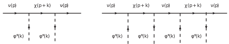
Figure 5: $s-$ channel $\nu-\phi$ interaction processes at the tree level (left) and at the next order with two $\phi$ being absorbed and emitted (right). The $u-$channel amplitude corresponds to diagrams with intersecting scalar lines.

Explanation of values of neutrino masses implies that $r_{\chi}\gg d$ in contrast to the standard case ($r_{W}\ll d$) which may testify that neutrino interactions with many $\phi$ can be important (especially if both $\phi$ and $\phi^{*}$ are around). So, one should consider processes with more than one $\phi$ being absorbed and emitted:

$$\nu\phi\rightarrow\nu\phi,\,\,\,\nu\phi\phi\rightarrow\nu\phi\phi,\,\,\,\nu\phi\phi\phi\rightarrow\nu\phi\phi\phi,\,\cdots\,$$

as shown in Fig. 5. The corresponding diagrams contain alternate propagators of $\chi$ and $\nu$ with $\phi$ vertices.

Let us consider, for definiteness, the case $\epsilon=-1$ when the $s-$channel contributes only. In the presence of two $\phi$ interactions $(\nu\phi\phi\rightarrow\nu\phi\phi)$ , the amplitude picks up an additional factor

$$\zeta=\lambda\frac{n_{\phi}}{m_{\phi}}\frac{\not{p}\not{p}_{\chi}}{p^{2}(p_{\chi}^{2}-m_{\chi}^{2})}=\Delta m_{\rm atm}^{2}\frac{\not{p}(\not{p}+\not{k})}{p^{2}(p_{\chi}^{2}-m_{\chi}^{2})}\,,$$ (37)

which should act eventually on the neutrino spinor $u_{L}$ to the right. Permuting $\not{p}$ and $\not{k}$, and using Eq. (29), we obtain

$$\zeta=\Delta m_{\rm atm}^{2}\frac{p^{2}+2(pk)-m_{\phi}\tilde{V}}{p^{2}(p_{\chi}^{2}-m_{\chi}^{2})}.$$ (38)

(The corrected potential $\tilde{V}$ is determined in eq. (32).) The dispersion relations reads $p^{2}=2VE+V^{2}\approx 2VE$. The other term $2(pk)=2Em_{\phi}$, and consequently,

$$\zeta\approx\frac{\Delta m_{\rm atm}^{2}}{p_{\chi}^{2}-m_{\chi}^{2}}=\frac{V}{m_{\phi}}=\Sigma_{1}\,.$$ (39)

Thus, the perturbativity condition $\zeta\ll 1$ coincides with the condition of smallness of WF renormalization (see (32)). This is not accidental since the neutrino WF renormalization is described through absorption and emission of multiple $\phi$, and therefore is described by the same diagram as Fig. 5 (right). Similarly, one can show the equivalence of perturbation conditions for $\epsilon=1$ and $\epsilon=0$.

Formally, resummation of the diagram with various number of insertions gives

$$V_{\rm resum}=\frac{V}{1+\zeta}\,,$$ (40)

which can lead to an additional suppression of the potential. As we saw, perturbativity holds above resonance. Below resonance $\zeta\simeq\Delta m_{\rm atm}^{2}/m_{\chi}^{2}\gg 1$ (for $\epsilon=-1$), so the result cannot be estimated reliably. However, below resonance, $\zeta$ does not depend on $E$ and therefore resummation should not produce an energy dependence of $V$ at least for $\epsilon\neq 0$. Hence, one expects a decrease of the effective mass-squared with $E$ simply due to multiplication of the potential by $(2E)$.

The convergence of this series of interactions can be tested by checking whether the $n-$th term of the series diverges. For a real field, the $n-$th term in the series gets a contribution of $n!$ from the different $\phi$ permutations. This cancels with the factor of $(1/n!)$ from the exponential, giving $(1/n!)\,n!\zeta^{n}=\zeta^{n}$. This series sum leads to $1/(1+\zeta)$, which is convergent. For a complex field, the number of permutations allowed are $(n/2)!$ for $\phi$ and $\phi^{*}$ respectively. This leads to a factor of $(1/n!)\,(n/2)!(n/2)!\zeta^{n}$ in the $n-$th term. Therefore, for a complex $\phi$, the series convergence is better due to an extra suppression by $n$.

III.4 The $\nu-\chi$ mixing due to scattering

Interaction (1) in a medium composed of the cold gas of scalars also produces $\nu_{L}-\chi^{c}_{L}$ mixing. The mixing is generated by off-diagonal potential in the space of states $(\nu,\chi^{c}_{L})$ which is proportional to the amplitude of forward off-diagonal scattering. The amplitude in the unit of length equals

$$A_{\alpha k}(x)=g_{\alpha k}\langle\chi^{c}_{kL}|\chi_{kR}\rangle\sum_{j=1\div n_{\phi}}\langle\chi_{kR}(p_{\chi})|\,\bar{\chi}_{k}(x)\nu_{\alpha}(x)\phi^{*}(x)\,|\nu_{L}(p_{\nu})\phi^{*}(p_{j})\rangle\,,$$ (41)

where summation proceeds over scatterers on the unit of length. Taking into account that $\langle\chi^{c}_{kL}|\chi_{kR}\rangle=m_{\chi k}/2E_{\chi}$ the explicit computations give the off-diagonal potential

$$V_{\alpha k}(x)=\frac{m_{\chi k}}{2E_{\chi}}\frac{g_{\alpha k}}{\sqrt{2m_{\phi}}}e^{i(p_{\chi}-p_{\nu})x}\sum_{j=1\div n_{\phi}}e^{-ip_{j}x}.$$ (42)

For ${\bf x}=0$ and non-relativistic scalars, $E_{j}\simeq m_{\phi}+m_{\phi}v_{j}^{2}/2$, hence the sum in Eq.(42) equals for random phases

$$e^{-im_{\phi}t}\sum_{j=1\div n_{\phi}}e^{-im_{\phi}v_{j}^{2}t/2}\simeq e^{-im_{\phi}t+i\phi^{\prime}}\sqrt{n_{\phi}},$$ (43)

where $\phi^{\prime}$ is some residual phase.

Consequently, the off-diagonal potential equals

$$V_{\alpha k}(x)=e^{-im_{\phi}t+i\phi^{\prime}}\,g_{\alpha k}\frac{m_{\chi k}}{2E_{\chi}}\sqrt{\frac{n_{\phi}}{2\,m_{\phi}}}\,,$$ (44)

where we have taken $E_{\nu}=E_{\chi}$ which removes the phase in eq. (42) related to $\nu$ and $\chi$.

Now the Hamiltonian of complete system which includes active neutrinos and singlets $\chi_{k}$ in the basis $(\nu_{\alpha},\chi_{k}^{c})_{L}$ can be written in the block form as

$${\bf H}\approx\frac{1}{2E}\begin{bmatrix}\tilde{m}_{\alpha\beta}^{2}&e^{-im_{\phi}t+i\phi^{\prime}}g_{\alpha k}m_{\chi k}\sqrt{n_{\phi}/2m_{\phi}}\\ e^{im_{\phi}t-i\phi^{\prime}}g_{\alpha k}m_{\chi k}\sqrt{n_{\phi}/2m_{\phi}}&m_{\chi k}^{2}+\tilde{m}_{\chi k}^{2}\end{bmatrix},$$ (45)

where $\tilde{m}_{\chi k}$ is refractive contribution to the mass squared of $\chi$. Parameters $m_{\chi k}$, $\phi^{\prime}$ can be selected in such a way that feedback of the $\nu-\chi$ mixing on the active neutrino oscillations is small. We consider phenomenological consequences of this mixing in sect. IV.5.

III.5 Resonance production of $\chi$

We can also consider the resonant production $\nu\rightarrow\chi$ in the bath of cold scalar particles. The amplitude of transition $\nu(p)+\bar{\phi}(k)\rightarrow\chi(p_{\chi})$ is proportional to

$$g\phi_{0}\left(\frac{m_{\chi}}{2E_{\chi}}\right)\,\int dx\,e^{i(p+k-p_{\chi})x},$$ (46)

where the factor $m_{\chi}/2E_{\chi}$ follows from angular momentum conservation in the scalar field, which produces the flip $\chi_{R}\rightarrow\chi_{L}$. The amplitude of scalar field $\phi_{0}$ is given by number density of $\phi$.

Integration over infinite space-time volume leads to a delta-function signifying exact energy-momentum conservation $p+k=p_{\chi}$. For $k=(m_{\phi},0)$, in the limit $m_{\chi}\gg m_{\phi}$, energy-momentum conservation gives $E=p=m_{\chi}^{2}/2m_{\phi}$, which is exactly the resonance energy $E_{R}$, as defined in (3). The uncertainty in energy $\delta E$ related to $\chi$ decay, $\chi\rightarrow\bar{\phi}+\nu$, is negligible: it is given by the width $\Gamma_{\chi,k}=g^{2}m_{\chi}/8\pi$. For instance, for $m_{\chi}=10^{-5}$ eV and $g=10^{-12}$, we find $\Gamma_{\chi}=4\cdot 10^{-19}$ eV and $\delta E=\Gamma_{\chi}m_{\chi}/E\sim 10^{-30}$ eV.

Much bigger uncertainty arises from non-zero velocities of $\phi$ particles. The energy and momentum conservation laws give

$$p_{\chi} = p\pm m_{\phi}v\,,$$ (47)

$$p_{\chi} + \frac{m_{\chi}^{2}}{2p_{\chi}}=p+m_{\phi}+\frac{m_{\phi}v^{2}}{2}\,.$$ (48)

Here $\pm$ in the Eq. (47) reflects interval of possible changes of $\phi-$momentum. From Eq. (48), we find

$$E_{R}\approx p_{R}\approx\frac{m_{\chi}^{2}}{2m_{\phi}(1\pm v)}\,.$$ (49)

That is, the resonance peak acquires the width

$$\Delta E\simeq 2E_{R}v\,.$$

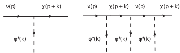
Figure 6: Left: $\nu-\chi$ transition at tree-level. Right: $\nu-\chi$ transition with additional $\phi$ interactions.

Furthermore, the transition $\nu\rightarrow\chi$ occurs in the $\phi-$medium which can be accounted in the lowest order by diagrams with two additional $\phi$ interactions in $\nu$ and $\chi$ lines, as shown in Fig. 6. This corresponds to renormalization of the $\nu-$ and $\chi-$ wave functions. The resulting two diagrams are identical giving corrections $\sim 2\Sigma_{1}$, where the factor of 2 is nothing but the Bose enhancement.

Finally, one should take into account the energy uncertainty in the propagating neutrinos which is determined by the process of their production. The uncertainty due to finite space-time integration in (46), given by inverse of baseline $L$ of experiment, $\sigma_{p}\sim 1/L$, is usually much smaller.

Thus, only a very small fraction of neutrinos $\simeq(2\cdot 10^{-3}-10^{-2})$ with energies close to the resonance energy can be converted into $\chi$. Far from the resonance $(E\gg E_{R}$ and $E\ll E_{R})$, $\chi$ is strongly virtual and can exist for a very short period of time $\sim 1/E\sim 10^{-20}\,$s.

IV Refraction in the classical field

Finding refractive mass in a cold gas via computations of the amplitudes of scattering on individual scatterers and summation over scatterers show some potential problems (unusual relation of scales, perturbativity, etc.). This may demand some other approach to computations.

IV.1 State of the scalar field

To explain neutrino masses, one should have a very large number density of $\phi$. If the occupation number of $\phi$ in the volume determined by the de Broglie wavelength is much bigger than 1, that is, $\lambda_{dB}^{3}n_{\phi}\gg 1$, a system of scalar particles can be treated as classical field $\phi_{c}$ (classicality condition) . Using that $n_{\phi}=\rho_{\phi}/m_{\phi}$, we obtain from the classicality condition,

$$m_{\phi}\ll 2\pi\left[\frac{\rho_{\phi}}{2\pi v^{3}}\right]^{1/4}.$$ (50)

For $v_{\rm vir}=10^{-3}$ and $\rho_{\phi}=\rho_{\odot}=0.3$ GeV/cm³, the equation (50) gives $m_{\phi}\ll 30$ eV. Then, for $E_{R}=0.01\,$MeV, Eq. (3) would lead to $m_{\chi}\ll 770\,$eV.

Such a scalar field can appear as an expectation value of the field operator in a coherent state of particles:

$$\phi_{c}(x)=\langle\phi_{\rm coh}|\hat{\phi}(x)|\phi_{\rm coh}\rangle\,,$$ (51)

where the coherent state $|\phi_{\rm coh}\rangle$ and its complex conjugate $|\bar{\phi}_{\rm coh}\rangle$ are defined in the Appendix A. These states could be formed in the early Universe via the misalignment mechanism.

The most general state is given by a linear combination of $|{\phi}_{\rm coh}\rangle$ and $|\bar{\phi}_{\rm coh}\rangle$,

$$|{\phi}_{\rm coh}^{\rm tot}\rangle=\cos\alpha|{\phi}_{\rm coh}\rangle+\sin\alpha|\bar{\phi}_{\rm coh}\rangle\,.$$ (52)

The corresponding field can be written as

$$\phi_{c}^{\rm tot}(x)=\langle{\phi}_{\rm coh}^{\rm tot}|\hat{\phi}(x)|{\phi}_{\rm coh}^{\rm tot}\rangle=\int\frac{d^{3}k}{(2\pi)^{3}}\frac{1}{\sqrt{2E_{k}}}\left[f_{a}^{\rm tot}(k)e^{-ikx}+f_{b}^{\rm tot}(k)e^{ikx}\right]\,.$$ (53)

$\phi_{c}^{\rm tot}(x)$ can also be parameterized as (for a detailed derivation, see Appendix A)

$$\phi_{c}^{\rm tot}(x)=F(x)e^{i\Phi}.$$ (54)

For the Hermitian conjugate, we have similarly

$$\phi_{c}^{{\rm tot}~{}\dagger}(x)=\bar{F}(x)e^{-i\bar{\Phi}}.$$ (55)

The factors $F^{2}$ and $\bar{F}^{2}$ are related to the corresponding contributions of $\phi$ to the energy density in the Universe:

$$F^{2}=\frac{\rho_{\phi}}{m_{\phi}^{2}},~{}~{}~{}\bar{F}^{2}=\frac{\rho_{\bar{\phi}}}{m_{\phi}^{2}}\,.$$ (56)

For a real field, we have $F(x)=\bar{F}(x)$ and $\tan\Phi=0$.

IV.2 Decoherence and strength of the scalar field

Even if at the moment of creation, the coherent state has $k\simeq 0$ and $E\simeq m_{\phi}$, in the course of DM halo formation (virialization), due to gravitational interactions, $\phi$ particles acquire a velocity distribution dispersion width $v_{\rm vir}$. In our Galaxy, the virialized velocities $v_{\rm vir}\simeq 10^{-3}$, and corresponding momenta $k=m_{\phi}v_{\rm vir}$. This determines the distributions functions of $\phi$ particles, described through $f(k)$ in (53). Due to dispersion of velocity, different $\phi$ acquire different momenta and energies, and consequently phases, which lead to decoherence. This appears as a suppression of the coherent component of the fields due to integration over momenta in (53).

For a given spatial point, the phase difference between different modes equals

$$\Delta\phi=\Delta Et\simeq E_{\rm vir}t=\frac{1}{2}m_{\phi}v_{\rm vir}^{2}t\,.$$ (57)

When $\Delta\phi\sim 2\pi$, coherence is lost. This gives for coherence time

$$t_{\rm coh}\simeq\frac{4\pi}{m_{\phi}v_{\rm vir}^{2}}=8\cdot 10^{-9}\,{\rm s}\left(\frac{\rm eV}{m_{\phi}}\right).$$ (58)

In reality, the time is bigger since $v_{\rm vir}$ increases in the process of virialization. For $m_{\phi}=10^{-12}\,{\rm eV},\,10^{-16}\,{\rm eV},\,10^{-20}\,{\rm eV}$, we obtain $t_{\rm coh}=8\cdot 10^{3}\,{\rm s},\,\,8\cdot 10^{7}\,{\rm s},\,\,8\cdot 10^{11}\,{\rm s}$ respectively. This implies that the field decoheres already during virialization. One can also compute the distance travelled by $\phi$ before decoherence takes over:

$$x_{\rm coh}\simeq\frac{4\pi}{m_{\phi}v_{\rm vir}}=5\cdot 10^{8}\,{\rm cm}\,\left(\frac{5\cdot 10^{-10}~{}{\rm eV}}{m_{\phi}}\right).$$ (59)

Thus, only for very tiny masses of $\phi$, coherence can be maintained over cosmological time.

In fact, for non-relativistic $\phi$, the scalar field does not vanish completely due to decoherence. The “residual" classical field will exist even for $t\rightarrow\infty$. Let us consider a unit volume at some spatial point and substitute the integration over momenta in (53) by summation:

$$\phi_{c}^{\rm tot}(x)\approx\frac{1}{\sqrt{2m_{\phi}}}\sum_{k}\left[f_{ak}e^{-ikx}+f_{bk}e^{ikx}\right].$$ (60)

Taking ${\bf x}=0$ and $E_{k}\simeq m_{\phi}+m_{\phi}v_{k}^{2}/2$, we obtain

$$\phi_{c}^{\rm tot}(x)=\frac{1}{\sqrt{2m_{\phi}}}\left[e^{-im_{\phi}t}\sum_{k}e^{-im_{\phi}v_{k}^{2}t/2}+e^{im_{\phi}t}\sum_{k}e^{im_{\phi}v_{k}^{2}t/2}\right].$$ (61)

For random phases in the exponents under sums, we have $\sum_{k}e^{im_{\phi}v_{k}^{2}t/2}=\sum_{k}e^{-im_{\phi}v_{k}^{2}t/2}\approx\sqrt{n}$, and therefore

$$\phi_{c}^{\rm tot}(t)\sim\sqrt{\frac{n_{\phi}}{m_{\phi}}}\cos m_{\phi}t\,.$$ (62)

The amplitude matches the field strength used in the cold gas computations. In addition, time variations of the field appear which have been studied extensively in a number of papers Berlin:2016woy ; Krnjaic:2017zlz ; Brdar:2017kbt ; Capozzi:2018bps ; Dev:2020kgz ; Losada:2021bxx ; Huang:2021kam ; Chun:2021ief ; Dev:2022bae ; Huang:2022wmz ; Davoudiasl:2023uiq ; Losada:2023zap ; Gherghetta:2023myo .

IV.3 Hamiltonian of propagation

The interaction (1) in the presence of non-zero expectation value of $\phi$ generate mass terms in the same way as the VEV of Higgs field generates masses in the Standard Model

$$\mathcal{L}\supset\sum_{k}g_{\alpha k}{\phi}_{c}^{{\rm tot}~{}\dagger}\bar{\chi}_{kR}\nu_{\alpha L}+\sum_{k}g_{\alpha k}^{*}\phi_{c}^{\rm tot}\bar{\nu}_{\alpha L}\chi_{kR}\,.$$ (63)

Notice that our consideration of evolution differs from that in Chun:2021ief . The resulting mass matrix in the basis of 3 flavor neutrino states and two mediators with definite Majorana masses: $(\nu_{f},\chi_{L})^{T}=(\nu_{e},\nu_{\mu},\nu_{\tau},\chi_{1},\chi_{2})^{T}$, where $\chi_{L}\equiv(\chi_{R})^{c}$, can be written as

$${\bf M}=\begin{bmatrix}0~{}~{}~{}~{}&g_{\alpha k}{\phi}_{c}^{{\rm tot}~{}\dagger}\\ g_{\alpha k}{\phi}_{c}^{{\rm tot}~{}\dagger}~{}~{}~{}~{}&{\rm diag}(m_{\chi k})\end{bmatrix}\,,~{}~{}~{}\alpha=e,\mu,\tau,~{}~{}~{}k=1,2.$$ (64)

The Hamiltonian of evolution is given by

$${\bf H}\approx\frac{1}{2E}{\bf M}{\bf M}^{\dagger}=\frac{1}{2E}\begin{bmatrix}\bar{F}^{2}\sum_{k}g_{\alpha k}g_{\beta k}^{*}~{}~{}~{}&g_{\alpha k}\bar{F}m_{\chi k}e^{-i\bar{\Phi}}\\ g_{\alpha k}^{*}\bar{F}^{*}m_{\chi k}e^{i\bar{\Phi}}~{}~{}~{}&\bar{M}_{\chi}^{2}\end{bmatrix},$$ (65)

where a common term proportional to the identity matrix is omitted and $\bar{F},\,\bar{\Phi}$ are defined in (54). Here

$$\bar{M}_{\chi}^{2}=\begin{bmatrix}\bar{F}^{2}\sum_{\alpha}|g_{\alpha 1}|^{2}+m_{\chi 1}^{2}~{}~{}~{}&\bar{F}^{2}\sum_{\alpha}g_{\alpha 1}g_{\alpha 2}^{*}\\ \bar{F}^{2}\sum_{\alpha}g_{\alpha 2}g_{\alpha 1}^{*}~{}~{}~{}&\bar{F}^{2}\sum_{\alpha}|g_{\alpha 2}|^{2}+m_{\chi 2}^{2}\end{bmatrix}.$$ (66)

For antiparticles (basis $(\bar{\nu},\bar{\chi})^{T}$), the mass matrix equals according to (63)

$$\bar{\bf M}=\begin{bmatrix}0~{}~{}~{}~{}&g_{\alpha k}^{*}{\phi}_{c}^{\rm tot}\\ g_{\alpha k}^{*}{\phi}_{c}^{\rm tot}~{}~{}~{}~{}&{\rm diag}(m_{\chi k})\end{bmatrix}~{}~{}~{}~{}~{}\alpha=e,\mu,\tau,~{}~{}~{}k=1,2.$$ (67)

Consequently, the Hamiltonian can be obtained from (65) by the following substitution: $\bar{F}\rightarrow F\,\,$, $\bar{\Phi}\rightarrow{-\Phi}$.

The Hamiltonian of evolution (65) coincides with the Hamiltonian (45) computed for cold gas at energies above the resonance, if $\Phi=m_{\phi}t-\phi^{\prime}$. The $3\times 3$ block of active neutrinos in the Hamiltonian (65), as well as the off-diagonal mixing block have the same form as the matrix $\tilde{m}_{\rm asy}^{2}$ produced by refraction on a cold $\phi$ gas (12) at high neutrino energies. We call $\bar{F}^{2}\sum_{k}g_{\alpha k}g_{\beta k}^{*}$ the refractive mass-squared in this case. We discuss in details two major features of this Hamiltonian: (1) energy and space - time dependence of neutrino effective mass matrix, and (2) $\nu-\chi$ mixing and oscillations.

IV.4 Energy and space - time dependence of neutrino effective mass matrix

Refractive mass depends on the neutrino energy, in particular, it decreases with energy below the resonance. In contrast, the mass (65) generated by the expectation value of the coherent scalar field on the first sight, has no resonance and does not depend on energy. Such a behavior would correspond to $E_{R}\rightarrow 0$ and $m_{\chi}=0$. The controversy is resolved in the following way.

The coherent field $\phi$ has time dependence and therefore can be considered as a wave with frequency $\sim m_{\phi}$. Therefore we can describe the process $\nu+\phi\rightarrow\chi$, as the $\nu\rightarrow\chi$ transition with the absorption of the $\phi$ wave. The transition occurs when frequency $m_{\phi}$ matches difference of energies of $\nu$ and final state $\chi$ and therefore has a resonance character. Below resonance, there is no on-shell $\chi$ production, therefore $\chi$ appears as a virtual particle, and the amplitude of its appearance decreases with increase of virtuality. Similarly, above the resonance, the appearance of $\chi$ decreases as $1/E$.

In fact, the wave component of the field $\phi(t,x)$ can be immediately treated as particle and therefore refraction effect can be computed with $\chi$ propagator in the same way as in a cold gas.

The scalar field depends on time, being proportional to $\bar{F}(x)$. Additional dependence on time is in the phase $\Phi$. For a real field, in the non-relativistic approximation $(k\simeq 0)$, the scalar mass squared goes as $4\bar{F}^{2}\cos^{2}m_{\phi}t$ Berlin:2016woy . Notice that $\bar{F}^{2}$ (${F}^{2}$) appears as a prefactor in the active neutrino block of the Hamiltonian. therefore its time variations do not change mixing of active neutrinos, but do change the effective masses squared. The scale of masses of neutrinos and antineutrinos, given by $\bar{F}^{2}$ and $F^{2}$, are the same for a real scalar field but can be different for a complex scalar field. This can imply that the refractive masses for neutrinos and antineutrinos can be different.

For very small $m_{\phi}$, the period of time variations, $(T_{\phi}\propto 1/m_{\phi})$, is very long - much longer than time of neutrino propagation in the oscillation setup. So, for description of oscillations one can take constant $\bar{F}^{2}(t_{0})$ and $F^{2}(t_{0})$ in a given moment $t_{0}$. This may not be true for cosmic neutrinos (SN or high energy neutrinos). However, $T_{\phi}$ can be smaller or comparable to the duration of neutrino experiments (several years). So, one can observe changes of extracted $\Delta m^{2}$ in the course of experiment. Non-observations of such changes put bounds on parameters of the field Berlin:2016woy ; Krnjaic:2017zlz ; Brdar:2017kbt ; Dev:2020kgz .

IV.5 The $\nu-\chi$ mixing and oscillations

According to the Hamiltonian in (65), there is $\nu_{\alpha}-\chi_{k}$ mixing, and therefore $\nu_{\alpha}-\chi_{k}$ oscillations. A convenient way to study this is to partially diagonalize the effective mass matrix (64). For definiteness, we will consider mixing of the neutrinos.

The off-diagonal submatrix of (64) has the form

$${\bf m}_{a\chi}=||g_{\alpha k}{\phi}_{c}^{tot~{}\dagger}||=\bar{F}e^{-i\bar{\Phi}}\begin{bmatrix}g_{1}~{}~{}~{}&0\\ g_{1}~{}~{}~{}&g_{2}\\ g_{1}~{}~{}~{}&-g_{2}\end{bmatrix}.$$ (68)

It can be diagonalized by a TBM rotation $(U_{TBM})$ of the active components only:

$$U_{TBM}{\bf m}_{a\chi}=e^{-i\bar{\Phi}}\begin{bmatrix}0~{}~{}~{}&0\\ m_{a1}~{}~{}~{}&0\\ 0~{}~{}~{}&m_{a2}\end{bmatrix},$$ (69)

where

$$m_{a1}\equiv\sqrt{3}g_{1}\,\bar{F}\,,~{}~{}~{}m_{a2}\equiv\sqrt{2}g_{2}\bar{F}\,,$$ (70)

and $a$ denotes the rotated basis of active neutrinos given by $\nu_{a}^{\prime}=U_{TBM}^{T}\nu_{\alpha}$. The Majorana mass matrix of $\chi$ remains diagonal in the transformation (69). Notice that one active (massless) state decouples, and in the limit $m_{\chi}\rightarrow 0$, the other states $(\nu_{a1},\nu_{a2})$ form two Dirac neutrinos with masses $m_{a1}$, $m_{a2}$.

After the rotation by (69) and decoupling of the $\nu_{e}^{\prime}$ state, the remaining 4-state system $(\nu_{a1},\nu_{a2},\chi_{1},\chi_{2})$ splits into two independent blocks of $(\nu_{a1},\chi_{1})$ and $(\nu_{a2},\chi_{2})$. The $(\nu_{a1},\chi_{1})$ mass matrix is given by

$${\bf M}_{a1}=\begin{bmatrix}0~{}~{}~{}&m_{a1}e^{-i\bar{\Phi}}\\ m_{a1}e^{-i\bar{\Phi}}~{}~{}~{}&m_{\chi 1}\end{bmatrix}.$$ (71)

The corresponding Hamiltonian reads

$${\bf H}_{a1}\approx\frac{1}{2E}{\bf M}_{a1}{\bf M}_{a1}^{\dagger}=\frac{1}{2E}\left(m_{a1}^{2}{\bf I}+\begin{bmatrix}0&m_{a1}m_{\chi 1}e^{-i\bar{\Phi}}\\ m_{a1}m_{\chi 1}e^{i\bar{\Phi}}&m_{\chi 1}^{2}\end{bmatrix}\right).$$ (72)

A similar Hamiltonian for $(\nu_{a2},\chi_{2})$ can be obtained by substitution $1\leftrightarrow 2$. The two pairs of states evolve independently leading to $\nu_{a1}\rightarrow\chi_{1}$ and $\nu_{a2}\rightarrow\chi_{2}$ oscillations.

The complex phase can be removed from the evolution equations by rephasing the neutrinos as $\nu_{a}^{\prime}\rightarrow e^{i\Phi(t)}\nu_{a}^{\prime}$. This leads to the appearance of an extra term in the Hamiltonian, proportional to the derivative of $\Phi$:

$${\bf H}_{a1}\approx\frac{1}{2E}\left(m_{a1}^{2}{\bf I}+\begin{bmatrix}0&m_{a1}m_{\chi 1}\\ m_{a1}m_{\chi 1}&m_{\chi 1}^{2}-2E\dot{\bar{\Phi}}\end{bmatrix}\right)\,.$$ (73)

Here $\dot{\bar{\Phi}}\simeq 0\div m_{\phi}$, where $0$ corresponds to symmetric background (real field), while $m_{\phi}$ is in the case of completely asymmetric background (for details, check Appendix A).

The terms in ${\bf H}_{ai}$ proportional to the unit matrices do not affect flavour evolution inside the pairs. However, they are important in the whole 5 neutrino system, in particular, in the relative evolution of the pairs. Diagonalization of the Hamiltonian (73) gives mass splittings and mixing:

$$\Delta m_{a1}^{2}=2\sqrt{(m_{\chi 1}^{2}-2E\dot{\bar{\Phi}})^{2}+m_{a1}^{2}m_{\chi 1}^{2}}\,\,,$$ (74)

$$\tan 2\theta_{a1}=\frac{2m_{a1}m_{\chi 1}}{m_{\chi 1}^{2}-2E\dot{\bar{\Phi}}}\,.$$ (75)

Since $m_{\chi 1}^{2}\ll m_{a1}^{2}\simeq\Delta m_{\rm sol}^{2}$, in (74), $m_{\chi 1}^{2}$ can be neglected. Therefore, for $\dot{\bar{\Phi}}=0$, we get

$$\Delta m_{a1}^{2}\geq 2\sqrt{\Delta m^{2}_{\rm sol}}m_{\chi 1}\,,~{}~{}~{}~{}\tan 2\theta_{a1}\simeq\frac{2\sqrt{\Delta m^{2}_{\rm sol}}}{m_{\chi 1}}\,.$$ (76)

For $m_{\chi 1}<10^{-3}\,$eV, the $\nu-\chi$ oscillations can be relevant for neutrinos from astrophysical sources such as the Sun, a core-collapse supernova (SN), as well as more distant sources. Furthermore, since $m_{a1}\gg m_{\chi 1}$, neutrinos turn out to be pseudo-Dirac particles with nearly maximal mixing of the active and sterile components.

Notice that the resonance character of refraction can be seen immediately from the Hamiltonian that describes oscillations. Indeed, according to (4.24) for $\dot{\Phi}=m_{\phi}$ the $\chi-\nu$ mixing becomes maximal at $E=m_{\chi}^{2}/2m_{\phi}$ which is nothing but the resonance energy in the potential $V$ due to scattering. So, the resonance here corresponds to oscillations with maximal depth. Change of the $\chi-\nu$ mixing parameter with energy corresponds to change of potential due to scattering: below the resonance $\tan 2\theta_{ai}$ converges to a constant value, while above the resonance it decreases as $1/E$.

The total mixing matrix which diagonalizes the mass matrix ${\bf M}$ in (64) is given by

$$U_{5}=\begin{bmatrix}U_{TBM}&0\\ 0&I\end{bmatrix}\times R_{24}(\theta_{a1})\times R_{35}(\theta_{a2}),$$ (77)

where $R_{24}$ and $R_{35}$ diagonalize the evolution equations of $(\nu_{a1},\chi_{1})$ and $(\nu_{a2},\chi_{2})$ pairs correspondingly. Explicitly, we get

$$U_{5}=\begin{bmatrix}\sqrt{2/3}&c_{a1}/\sqrt{3}&0&s_{a1}/\sqrt{3}&0\\ -1/\sqrt{6}&c_{a1}/\sqrt{3}&c_{a2}/\sqrt{2}&s_{a1}/\sqrt{3}&s_{a2}/\sqrt{2}\\ 1/\sqrt{6}&-c_{a1}/\sqrt{3}&c_{a2}/\sqrt{2}&-s_{a1}/\sqrt{3}&s_{a2}/\sqrt{2}\\ 0&-s_{a1}&0&c_{a1}&0\\ 0&0&-s_{a2}&0&c_{a2}\end{bmatrix}\,,$$ (78)

where $c_{a1,a2}\equiv\cos\theta_{a1,a2}$, and $s_{a1,a2}\equiv\sin\theta_{a1,a2}$.

Let us consider bounds arising from active to sterile oscillations of solar neutrinos. At low energies, $E<1$ MeV, usual matter effect can be neglected and the averaged $\nu_{e}$ survival probability equals

$$P_{ee}=\sum_{j}|U_{5ej}|^{4}=\frac{5}{9}-\frac{1}{18}\sin^{2}2\theta_{a1}.$$

Thus, for maximal mixing, $\sin^{2}2\theta_{a1}=1$, the oscillations of $\nu_{e}$ into $\chi$ reduce the probability by $1/18$ which is within the error bars. However, the effect at high energies (${}^{8}B$ neutrinos) is much stronger: $P_{ee}\approx 0.5\sin^{2}\theta_{12}\approx 0.15$ instead of 0.31, which is excluded.

A way to resolve this problem is to have $\Delta m^{2}_{a1}<10^{-12}{\,\rm eV}^{2}$ deGouvea:2009fp , so that oscillations into sterile components do not develop. In the case of a real field ($\dot{\Phi}=0$), this implies, according to Eq. (74), that

$$m_{\chi 1}\leq\frac{\Delta m^{2}_{a1}}{\sqrt{\Delta m^{2}_{\rm sol}}}\approx 10^{-10}\,{\rm eV}.$$ (79)

This bound is shown by the horizontal edge of the hatched region in Fig. 4.

In the case of maximal asymmetry, the condition of large oscillation length leads to

$$\dot{\Phi}\simeq m_{\phi}\leq\frac{\Delta m^{2}_{a1}}{4E}\approx 10^{-18}\,{\rm eV}.$$ (80)

The bounds in Eqs. (79) and (80) are consistent with what we had for refraction in the cold gas.

Another way to satisfy the solar bounds is to arrange for small mixing. If $\dot{\Phi}\simeq m_{\phi}$, and $E\dot{\Phi}\gg m_{\chi 1}^{2}$, we have, from (74) and (75),

$$\Delta m^{2}_{a1}\approx 4E\dot{\Phi}=4Em_{\phi},\,\,\,\tan 2\theta_{a1}=\frac{m_{\chi 1}\sqrt{\Delta m^{2}_{\rm sol}}}{Em_{\phi}},$$ (81)

and consequently, from the second equation,

$$\frac{m_{\chi 1}}{m_{\phi}}<\tan 2\theta_{a1}\frac{E}{\sqrt{\Delta m^{2}_{\rm sol}}}.$$ (82)

Requiring $\tan 2\theta_{a1}=10^{-2}$ for $E=1$ MeV, we obtain

$$\frac{m_{\chi 1}}{m_{\phi}}<10^{6}\,.$$ (83)

According to Fig. 4, this can be satisfied if $m_{\phi}\gtrsim 10^{-10}$ eV. This bound corresponds to the diagonal border of the hatched region in Fig. 4.

Notice that for $\dot{\Phi}=0$, we would get

$$m_{\chi 1}\geq\frac{2\sqrt{\Delta m^{2}_{\rm sol}}}{\tan 2\theta_{a1}}\,,\,\quad\tan 2\theta_{a1}=2m_{a1}/m_{\chi 1}<10^{-2}\,.$$ (84)

Therefore, $m_{\chi 1}\geq 1.6$ eV, and consequently, $\Delta m^{2}_{a1}\gtrsim 2.6\,$eV². These large values of $m_{\chi 1}$ are, however, in tension with bounds arising from big bang nucleosynthesis, as well as from observation of neutrinos from SN1987A and other cosmic sources (discussed in the next sections).

V Astrophysical and cosmological bounds on parameters

V.1 Cosmological evolution of refractive mass and structure formation

Decrease of the refractive mass-squared with energy below resonance allows to avoid (at least partially) the cosmological bound on the sum of neutrino masses. Since the DM density redshifts as ordinary non-relativistic matter $\sim(1+z)^{3}$, any neutrino mass sourced from the DM field grows in the early Universe. The current sum of neutrino masses equals $\sum m_{\nu}\approx\sqrt{\Delta m^{2}_{\rm atm}}$ in the case of normal mass hierarchy. Therefore, in the period of photon decoupling $(z\simeq 1000)$, the neutrino mass $m(z)$ becomes as large as $\mathcal{O}(10)\,$eV, thereby making the neutrinos non-relativistic. This will be in tension with the current Planck limit of $\sum m_{\nu}<0.12\,{\rm eV}$ from observations of the CMB as well as baryon acoustic oscillations Planck:2018vyg . The bound can be evaded for appropriate choice of the resonance energy since for energies below the resonance, the refractive neutrino mass decreases with energy and becomes small (see Fig. 3), if the picture described in sect. II is correct.

If the refractive mass squared in our solar system is $\tilde{m}^{2}$, then the average value of the mass in the Universe equals $\tilde{m}^{2}(0)=\xi\,\tilde{m}^{2}$, where $\xi^{-1}\simeq 10^{5}$ is the local overdensity of DM. Taking into account the energy dependence of the mass, we obtain at low energies according to (16),

$$\tilde{m}^{2}(0)=\xi\,\tilde{m}^{2}_{\rm asy}(0)\,y(\epsilon-y)=\xi\,\tilde{m}^{2}_{\rm asy}(0)\,\left(\frac{E(0)}{E_{R}}\right)\,\left[\epsilon-\frac{E(0)}{E_{R}}\right]\,,$$ (85)

where $E(0)$ is the energy in the present epoch. Due to redshift, we have $\tilde{m}^{2}_{\rm asy}(z)\propto n_{\phi}(z)\propto(1+z)^{3}$ and $E(z)=E(0)(1+z)$. Therefore the effective mass squared increased in the past as

$$\tilde{m}^{2}(z)=\xi\,\tilde{m}^{2}_{\rm asy}(0)\,(1+z)^{4}\,\left(\frac{E(0)}{E_{R}}\right)\,\left[\epsilon-\frac{E(0)}{E_{R}}(1+z)\right]\,.$$ (86)

If the asymmetry is large enough, so that the second term in brackets can be neglected, we obtain

$$\tilde{m}^{2}(z)=\xi\,\epsilon\,\Delta m_{\rm atm}^{2}\,(1+z)^{4}\,\left(\frac{E(0)}{E_{R}}\right)\,,$$ (87)

where we used $\tilde{m}^{2}_{\rm asy}(0)=\Delta m_{\rm atm}^{2}$. Eq. (87) gives expression for the resonance energy:

$$E_{R}=E(0)\,\xi\,\epsilon\,(1+z)^{4}\,\frac{\Delta m_{\rm atm}^{2}}{\tilde{m}^{2}(z)}\,.$$ (88)

Using the cosmological bound on sum of neutrino masses $\tilde{m}^{2}(z)\leq(\sum m_{\nu})^{2}$, we find, from (88), the lower bound

$$E_{R}\geq E(0)\,\xi\,\epsilon\,(1+z)^{4}\,\frac{\Delta m_{\rm atm}^{2}}{(\sum m_{\nu})^{2}}\,.$$ (89)

For $E(0)=3\,T_{\rm rel}=6.9\cdot 10^{-4}$ eV, $z=1000$ and $\sum m_{\nu}<0.12\,{\rm eV}$, this equation gives

$$E_{R}\geq 1.2\,\epsilon\,\,{\rm keV}.$$ (90)

For zero asymmetry $(\epsilon=0)$, according to (86),

$$\tilde{m}^{2}(0)=-\xi\,\tilde{m}^{2}_{\rm asy}(0)\left(\frac{E(0)}{E_{R}}\right)^{2}\,,$$ (91)

similar consideration gives

$$\tilde{m}^{2}(z)=\xi\,\Delta m_{\rm atm}^{2}\,(1+z)^{5}\,\left(\frac{E(0)}{E_{R}}\right)\,,$$ (92)

and consequently, the bound

$$E_{R}\geq E(0)\,\left[\xi\,(1+z)^{5}\right]^{1/2}\,\left(\frac{\sqrt{\Delta m_{\rm atm}^{2}}}{\sum m_{\nu}}\right)\,.$$ (93)

Numerically, for $z=1000$, Eq. (93) leads to $E_{R}\geq 28$ eV.

Notice that in this consideration we treated $\tilde{m}^{2}$ with respect to structure formation as usual VEV mass. What matters is the energy density in neutrinos and their group velocity, and these characteristics differ in the case of refractive mass.

Indeed, in our case $E=p+V(p)$, and the group velocity, following (13), equals

$$v_{g}=\frac{dE}{dp}=1+\frac{dV}{dp}\,,\qquad\frac{dV}{dp}\approx 1-\frac{\tilde{m}^{2}_{\rm asy}}{2E_{R}^{2}}\left[1-2\epsilon\frac{p}{E_{R}}\right]$$ (94)

in the lowest order in $p/E_{R}$. This should be compared with

$$v_{g}\approx 1-\frac{m^{2}}{2E^{2}}$$

in the usual case. Furthermore, the refractive mass squared depends on density perturbation. Therefore the cosmological bound should be reconsidered specifically for refractive masses taking into account its dependence on energy and density of DM.

V.2 Neutrino - Dark matter interactions

Astrophysical neutrinos interact with DM halos as well as DM in the intergalactic space along their path to the Earth. This leads to energy loss of the neutrinos and, consequently, to a suppression of their flux for a given spectra $\propto E^{-\gamma}$ with $\gamma>0$  Barranco:2010xt ; Reynoso:2016hjr ; Choi:2019ixb ; Ferrer:2022kei ; Cline:2022qld ; Carpio:2022sml ; Cline:2023tkp . This constrains $\nu-\phi$ interactions, and hence, parameters of our scenario.

The neutrino (inelastic) scattering proceeds due to $\chi$ exchange on $\phi^{*}$ ($s-$channel) and $\phi$ ($u-$channel) and is described by the same diagrams as refraction (see Fig. 1). However, in contrast to refraction, these contributions sum up incoherently. Below and above the resonance energy, the s-channel cross-section can be written as

$$\sigma_{\nu\bar{\phi}}=\begin{cases}\frac{g^{4}m_{\phi}E}{16\pi m_{\chi}^{4}}\,,&m_{\phi}\ll E\ll E_{R}\,,\\ \frac{g^{4}}{64\pi m_{\phi}E}\,,&E\gg E_{R}\,.\end{cases}\,$$ (95)

For the $u-$channel, the cross section is given by

$$\sigma_{\nu\phi}=\begin{cases}\frac{g^{4}m_{\phi}E}{8\pi m_{\chi}^{4}}\,,&m_{\phi}\ll E\ll E_{R}\,,\\ \frac{g^{4}}{32\pi m_{\phi}E}\left[-1+{\rm log}\left(\frac{2Em_{\phi}}{m_{\chi}^{2}}\right)\right]\,,&E\gg E_{R}\,.\end{cases}\,$$ (96)

The optical depth of neutrinos in $\phi-$ background equals

$$\tau\equiv\int(n_{\phi}\sigma_{\nu\phi}+\bar{n}_{\phi}\sigma_{\nu\bar{\phi}})\,dl_{\rm los}\,=\frac{1}{m_{\phi}}\int_{0}^{L}\left(\rho_{\phi}\sigma_{\nu\phi}+\bar{\rho}_{\phi}\sigma_{\nu{\bar{\phi}}}\right)\,dl_{\rm los}\,,$$ (97)

The integration proceeds along the line of sight $l_{\rm los}$ from the source to the Earth. Therefore, the experimental bound on suppression of the neutrino flux from the source at distance $L$ is transformed into a bound on the ratio of the total cross-section and $m_{\phi}$. This, in turn, gives an upper bound on $g$ as function of $m_{\phi}$ for different values of $m_{\chi}$. To obtain such a dependence for a given experiment, which detects neutrinos of the energy $\sim E$, we define the resonance value of $m_{\phi}$:

$$m_{\phi}^{R}\equiv\frac{m_{\chi}^{2}}{2E}\,.$$ (98)

Notice that with increase of energy $E$, the mass $m_{\phi}^{R}$ shifts to smaller values. Then Eqs. (95) and (96) give the upper bounds on $g$ as a function of the parameters $m_{\phi}$, $m_{\chi}$ and energy as follows. For a fixed $\rho$, in the range $m_{\phi}\ll m_{\phi}^{R}$, which corresponds to $E\ll E_{R}$, we find that $g\propto m_{\chi}/E^{1/4}$, while for $m_{\phi}\gg m_{\phi}^{R}$ ($E\gg E_{R}$), we get $g\propto m_{\phi}^{1/2}E^{1/4}$. These dependences can be seen in the IceCube and SN constraints in Fig. 7, which will be discussed below.

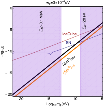
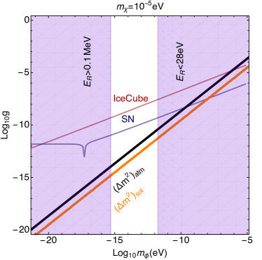
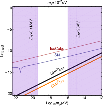
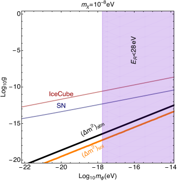
Figure 7: The bounds and regions required for explanation of oscillation data by refraction in the $g-m_{\phi}$ plane for different values of $m_{\chi}$. We take $\rho_{\phi}=\rho_{\odot}$. The values of $\Delta m_{\rm atm}^{2}$ and $\Delta m_{\rm sol}^{2}$ are reproduced along the black and orange lines correspondingly. Shown are the upper bounds on $g$ as function of $m_{\phi}$ from observations of IceCube high energy neutrinos (red) and neutrinos from SN1987A (blue). Mauve vertical bands correspond to $E_{R}>0.1$ MeV, excluded by oscillation data, and $E_{R}<28$ eV, excluded by cosmological bound on sum of neutrino masses.

In our computations, we use the DM density distribution in the Milky Way described by a Navarro-Frenk-White (NFW) profile Navarro:1996gj . The cosmological DM density in the Universe redshifts like as $\rho_{\rm EG}(z)=\xi\rho_{\odot}(1+z)^{3}$. The total DM density is given as a sum of these two terms, that is, $\rho_{\phi}+\bar{\rho}_{\phi}=\rho_{\rm gal}+\rho_{\rm EG}$. Assuming that the spatial distributions of $\phi$ and $\bar{\phi}$ are the same $(\rho_{\phi}\sim\bar{\rho}_{\phi})$, we can write expression for the optical depth as

$$\tau=\frac{1}{2m_{\phi}}\left[(1+\epsilon)\sigma_{\nu\phi}+(1-\epsilon)\sigma_{\nu{\bar{\phi}}}\right]\int\left(\rho_{\rm gal}+\rho_{\rm EG}\right)\,dl_{\rm los}\,.$$ (99)

For a symmetric medium ($\epsilon=0$), the line-of-sight integral over the galactic component $\rho_{\rm gal}$ yields

$$\int\rho_{\rm gal}\,dl_{\rm los}=2.6\times 10^{22}\,~{}{\rm GeV}/{\rm cm}^{2}\,.$$ (100)

The extra-galactic contribution to $\tau$ is given by integration over the redshift as

$$\int\rho_{\rm EG}\,dl_{\rm los}=\int_{0}^{z_{0}}\frac{\rho_{\rm EG}}{H_{0}(1+z)\sqrt{\Omega_{\Lambda}+\Omega_{m}(1+z)^{3}}}\,dz\,,$$ (101)

where $H_{0}=67.4$ km/s/Mpc, $\Omega_{\Lambda}=0.685$ and $\Omega_{m}=0.315$ Planck:2018vyg .

V.3 Bounds from SN1987A and IceCube neutrinos

Let us apply the formulae of subsection V.2 to existing observations of astrophysical neutrinos.

1. SN1987A. Requiring that the suppression of the $\mathcal{O}(10)\,{\rm MeV}$ neutrino flux from SN1987A Hirata:1987hu ; Hirata:1988ad ; Bionta:1987qt ; Alekseev:1988gp at a distance of around $50\,$ kpc from the Earth is no more than a factor 0.1 gives $\tau\leq 2.3$. Using only $\rho_{\rm gal}$ in Eq. (99), we obtain

$$\frac{\sigma_{\nu\phi}+\sigma_{\nu{\bar{\phi}}}}{m_{\phi}}\lesssim 9\times 10^{-23}\,{\rm cm}^{2}/{\rm GeV}\,.$$ (102)

2. IceCube. IceCube has reported the observation of a $290\,$TeV cosmic neutrino in association with the $\gamma$-ray blazar TXS 0506+056 at a redshift $z_{0}=0.3365\pm 0.0010$, corresponding to a distance of $~{}1421\,$Mpc IceCube:2018dnn . Now, the requirement $\tau\leq 2.3$ gives

$$\frac{\sigma_{\nu\phi}+\sigma_{\nu{\bar{\phi}}}}{m_{\phi}}\lesssim 7\times 10^{-23}~{}\,{\rm cm}^{2}/{\rm GeV}\,.$$ (103)

Using the expressions for $\sigma_{\nu\phi}$ and $\sigma_{\nu{\bar{\phi}}}$, we convert the bounds (102) and (103) into upper bounds on $g$ as a function of $m_{\phi}$ (see Fig. 7). For simplicity, we assume that $m_{\chi 1}=m_{\chi 2}=m_{\chi}$. The bounds agree with those obtained in Choi:2019ixb . Along the black and orange lines, the observed solar and atmospheric neutrino mass-squared difference can be obtained using refractive masses only.

The vertical shaded regions in mauve show the constraints arising from the condition $28\,{\rm eV}\leq E_{R}\leq 0.1\,{\rm MeV}$, as discussed in Sec.II.2. According to Fig. 7, values of the parameters which satisfy the existing bounds and allow to reproduce oscillation data are in the following ranges:

$$m_{\chi}=\left(3\cdot 10^{-9}\div 10^{-4}\right)~{}{\rm eV},~{}~{}~{}m_{\phi}=\left(10^{-19}\div 10^{-10}\right)~{}{\rm eV},~{}~{}~{}g=10^{-18}\div 10^{-7}\,.$$ (104)

V.4 Cosmological constraints on $\nu-\chi$ mixing

The relic density of $\phi$ can be set by the misalignment mechanism Preskill:1982cy ; Abbott:1982af ; Dine:1982ah . According to this mechanism, $\phi$ is initially displaced from the minimum of the potential. The field remains constant due to Hubble friction. It starts oscillating at temperatures below $T_{H}$, determined by the equality $m_{\phi}=3H(T_{H})$, where $H$ is the Hubble parameter. For $T<T_{H}$, the DM redshifts as non-relativistic matter so that its energy density varies as $T^{3}$  Dev:2022bae :

$$\rho_{\phi}(T)=\rho_{\phi}(T_{0})\left(\frac{g_{*}(T_{0})}{g_{*}(T)}\right)\left(\frac{{\rm min}(T,T_{H})}{T_{0}}\right)^{3}\,.$$ (105)

Here $T_{0}=2.72\,$K is the present temperature of the CMB. Consequently, the DM density increases with temperature upto $T$ at which $m_{\phi}=3H$, and then remains constant.

In the presence of the classical field $\phi_{c}$, the mediator $\chi$ mixes with $\nu$ and therefore can be produced from $\nu-\chi$ oscillations in the early Universe through the Dodelson-Widrow mechanism Dodelson:1993je . The distribution of $\chi$ can be computed through the following semi-classical Boltzmann equation,

$$\frac{\mathrm{d}f_{\chi i}}{\mathrm{d}T} =- \frac{\Gamma_{\nu}}{4HT}\frac{\left(\Delta m^{2}_{ai}\sin\,2\theta_{ai}\right)^{2}}{\left(\Delta m^{2}_{ai}\sin\,2\theta_{ai}\right)^{2}+E^{2}\Gamma_{\nu}^{2}+\left(\Delta m^{2}_{ai}\cos 2\theta_{ai}-2EV\right)^{2}}\,\,f_{\nu_{a}}\,.$$ (106)

Here $\Delta m^{2}_{ai}$ and $\theta_{ai}$ are oscillation parameters in the $(\nu_{a}^{\prime},\chi_{i})$ system as defined in (74), (75). In Eq. (75), the thermal scattering rates of neutrinos $\Gamma_{\nu}$ and the effective forward scattering matter potential in a symmetric medium are given by Abazajian:2001nj

$$\Gamma_{\nu} = \frac{7\pi}{24}G_{F}^{2}ET^{4}\,,$$ (107)

$$V = -\frac{14\sqrt{2}\pi^{2}}{45}G_{F}ET^{4}\left(\frac{1}{M_{Z}^{2}}+\frac{2}{M_{W}^{2}}\right)\,.$$ (108)

Eq. (106) can be solved numerically to obtain the contribution of $\chi$ to extra radiation around the time of big-bang nucleosynthesis (BBN):

$$\Delta N_{\rm eff}=\frac{\rho_{\chi}}{\rho_{\nu}}\,,$$ (109)

where $\rho_{\chi,\nu}$ is the energy density associated with $\chi$ and $\nu$ respectively. The current state-of-the-art limit is $\Delta N^{\rm BBN}_{\rm eff}<0.5$ Gariazzo:2021iiu .

The choices of $g_{e2}=0$ in the TBM form imply that the $\nu_{e}-\chi_{2}$ mixing is zero, $\sin 2\theta_{e2}=0$, therefore $\chi_{2}$ cannot be produced by $\nu_{e}$ through oscillations; however, oscillations $\nu_{\mu,\tau}\to\chi_{2}$ can happen. Similarly, $\chi_{1}$ can be produced by all three neutrino flavours in the early Universe. This can be suppressed by requiring that $\nu-\chi$ oscillations do not develop before $T\sim 1\,{\rm MeV}$, thereby avoiding the BBN bounds. This can be satisfied if $\Delta m^{2}_{ai}/(2T)<H$ at around $T=1\,{\rm MeV}$. This gives $\Delta m^{2}_{ai}<10^{-9}\,{\rm eV}^{2}$. For a real $\phi$, according to (79), this leads to $m_{\chi}<10^{-9}\,{\rm eV}$, assuming that the refractive mass stops growing at $z=1000$ and is constant till the BBN epoch. This bound is weaker than that from solar neutrinos. Another way of evading the BBN bound is to consider small mixing angles $\theta_{ai}$, as given in (81). This would also prevent $\chi$ from being populated in early Universe from $\nu-\chi$ mixing.

Other constraints can exist for the classical field component of ultralight dark matter. The wavelike nature of such a dark matter candidate can lead to wave interference, causing fluctuations which heat up stellar objects. Observations of ultrafaint dwarf (UFD) galaxies have been used to rule out masses of fuzzy dark matter $m_{\phi}<10^{-19}\,{\rm eV}$ Dalal:2022rmp . However, this constraint can be evaded by allowing for $\phi$ to produce only a fraction of the DM relic density. Hence we do not discuss these bounds further.

Combining both astrophysical and cosmological bounds considered in this section (see also Fig. 4 and Fig. 7), we obtain viable ranges of parameters,

$$m_{\chi}\simeq(1\div 3)\cdot 10^{-4}~{}{\rm eV},~{}~{}~{}m_{\phi}\simeq 10^{-10}\div 10^{-9}~{}{\rm eV},~{}~{}~{}g\simeq 10^{-10}\div 10^{-9}\,.$$ (110)

They are in agreement with the numbers found in Choi:2020ydp . Another possible region is given by

$$m_{\chi}\simeq 10^{-10}~{}{\rm eV},~{}~{}~{}m_{\phi}\simeq 10^{-21}~{}{\rm eV},~{}~{}~{}g\simeq 10^{-20}\,.$$ (111)

VI Discussion and Conclusion

We explored in detail a possibility that neutrino oscillation results can be explained by interactions of massless neutrinos with ultralight scalar dark matter $\phi$. The scheme includes light fermionic mediator $\chi$ with mass $m_{\chi}\gg m_{\phi}$ and Yukawa coupling $g\bar{\chi}\nu\phi^{*}+h.c.$. Explanation of neutrino oscillations require the existence of at least two mediators.

We introduced the refractive neutrino mass squared, $\tilde{m}^{2}$, generated dynamically via refraction of neutrinos in the $\phi-$background. Properties of the refractive masses and their phenomenological consequences are studied. We obtained constraints on parameters of the scheme $(g,m_{\phi},m_{\chi})$ from neutrino oscillations, as well as astrophysical and cosmological observations.

Properties of the refractive mass depend on the state of the scalar background, in particular, on whether it appears as a cold bath of scalar particles or as a classical scalar field representing a coherent state of scalar bosons.

In the case of a cold bath of bosons, the refraction has a resonance dependence on energy related to $\chi$ production. Above the resonance, $E>E_{R}=m_{\chi}^{2}/(2m_{\phi})$, the refractive mass has the same properties as the usual vacuum mass: it does not depend on energy, being equal for neutrinos and antineutrinos. $E_{R}$ should be much smaller than the lowest energy of detected neutrinos for which no dependence of masses and mixing on energy is found. This gives the upper bound $E_{R}\leq 0.1\,{\rm MeV}$. Below resonance $(E<E_{R})$, the refractive mass decreases with energy. For C-asymmetric background, it decreases as $\epsilon/E$, where $\epsilon$ quantifies the asymmetry, while in a C-symmetric medium (real field), the decrease is stronger: $1/E^{2}$. This can lead to very small (unobservable) effective neutrino mass in beta-decay experiments like KATRIN.

The key difference of the refractive mass from the usual VEV-induced mass is that it is proportional to the number density of particles of the background and therefore its value increased in the past due to redshift. Decrease of $\tilde{m}^{2}$ with energy below the resonance allows to satisfy the cosmological bound on the sum of neutrino masses obtained from structure formation. The bigger the resonance energy, the stronger is the decrease of mass. For C-symmetric background we obtain from cosmology the lower bound $E_{R}>28\,{\rm eV}$. Thus, $E_{R}\in[30-10^{5}]$ eV. For completely asymmetric background $(\epsilon=1)$, the lower bound is much stronger: $E_{R}>1.2\,{\rm keV}$.

For a fixed value of the mediator mass $m_{\chi}$, the allowed interval for the resonance energy is transformed onto the interval for the scalar mass. The bounds on the coupling $g$ as function scalar mass $m_{\phi}$ follow from scattering of astrophysical neutrinos (high energy cosmic neutrinos and neutrinos from SN1987A) on the background scalars. This scattering leads to energy loss of the neutrinos, and suppresses their flux. Combining both astrophysical and cosmological bounds constrain the viable ranges of parameters as $m_{\chi}\simeq(1\div 3)\cdot 10^{-4}~{}{\rm eV},~{}~{}~{}m_{\phi}\simeq 10^{-10}\div 10^{-9}~{}{\rm eV},~{}~{}~{}g\simeq 10^{-10}\div 10^{-9}\,.$ Another possible region is given by $m_{\chi}\simeq 10^{-10}~{}{\rm eV},~{}~{}~{}m_{\phi}\simeq 10^{-21}~{}{\rm eV},~{}~{}~{}g\simeq 10^{-20}\,.$ For these values of parameters, the refractive mass can reproduce the value $\Delta m^{2}_{\rm atm,sol}$ in the lowest order of perturbation theory,

Very small mass of $\phi$ means that these particles have a much larger de-Broglie wavelength than the radius of interaction, which in turn, is much larger than the distance between the scatterers. This indicates that multiple neutrino interactions with $\phi$ may become important. We find that for parameters required to reproduce the observed neutrino masses, the perturbation theory related to multiple $\phi$ interactions is broken at low energies. The perturbation parameter $\zeta$ increases with decrease in energy as $\zeta\sim 1/E$, and $\zeta(E_{\rm p})\simeq 1$ is achieved at energies above resonance: $E_{\rm p}\gg E_{R}$. For a C-symmetric medium, $E_{\rm p}$ can be smaller than 0.1 MeV so that results obtained for $\tilde{m}^{2}$ in the lowest approximation remain valid. Perturbativity can break down for energies close to the resonance energy. Below resonance, $\zeta$ is independent of energy, so we expect the refractive neutrino mass to decrease with energy as before, thus satisfying the cosmological bound. Qualitatively, in the non-perturbative situation, the dependence of $\tilde{m}^{2}$ on $E$ can be similar to the perturbative one in the lowest order. Also due to the $\bar{\chi}\nu\phi$ coupling, the off-diagonal $\chi^{c}-\nu$ potentials are generated, which lead to $\chi^{c}-\nu$ mixing and oscillations.

Notice that at the condition $d\ll r_{\chi}$, the standard computations of the local potentials $V_{\alpha,\beta}$ with integration over the infinite spatial coordinates may become problematic.

In the case of a background described by classical scalar field (coherent state of scalar bosons), the coupling $g\bar{\chi}\nu\phi^{*}$ generates off-diagonal mass terms for $\nu$ and $\chi$, that is, the off-diagonal elements of the mass matrix $M$. Then the mass matrix squared, $MM^{\dagger}$, has the $3\times 3$ active neutrino block proportional to that obtained for refractive mass squared at high energies. This mass has no explicit energy dependence and therefore differs from refractive mass at low energies. However, the $\phi$ field, and consequently, the neutrino mass squared have time dependence which effectively reproduces the resonance features. The resonance in the refractive mass corresponds to resonance in $\nu-\chi$ oscillations.

We find that at high energies, the Hamiltonian of evolution of whole the system of $(\nu,\chi^{c})$ is essentially the same for coherent classical field and a cold gas of scalars.

The $\nu-\chi$ mixing and oscillations are relevant for neutrinos from astrophysical sources. The strongest constraints arise from solar neutrinos. This can be evaded in two ways. For $m_{\chi}<\sqrt{\Delta m^{2}_{\rm sol}}$, neutrinos are pseudo-Dirac and the mixing between $\nu$ and $\chi$ is maximal. In this case, the solar neutrino constraint can be evaded by not allowing $\nu-\chi$ oscillations to develop over the solar baseline. For a real $\phi$, this imposes the bound $m_{\chi}<10^{-10}\,{\rm eV}$. Another way of avoiding these bounds is to arrange for small $\nu-\chi$ mixing. The mixing is given by $m_{\chi}\sqrt{\Delta m^{2}_{\rm sol}}/(Em_{\phi})$ and can be suppressed for $m_{\chi}<10^{6}\,m_{\phi}$ at $E=1\,{\rm MeV}$. This condition is consistent with the other constraints for $m_{\phi}\gtrsim 10^{-10}\,{\rm eV}$.

With the identification $\phi=\sqrt{n_{\phi}/m_{\phi}}$, both the states of the background can lead to the same effective neutrino masses at observable energies. In the case of a real $\phi$ or in the presence of a coherent state of $\phi$ and $\phi^{*}$, the neutrino refractive masses can show time-variations.

The neutrino oscillation phenomena are directly related to refraction on the dark matter background. The neutrino mass can change periodically with time and can be different in different spatial points. It may show energy dependence at low energies. All these features should be subject of experimental searches.

The masses of the new fermions $\chi$ need to be introduced by some high-scale physics. It may be related to some Planck scale physics, so that $m_{\chi}\sim v_{EW}^{2}/M_{Pl}$. Alternatively it can be generated by some refraction effect in the dark sector.

In conclusion, the nature of neutrino mass may be related to the nature of dark matter and the cosmological evolution of the Universe.

Appendix A General formalism for a coherent field

In this appendix, we derive the general formalism for a coherent field. We consider a complex scalar field operator

$$\hat{\phi}(x)=\int\frac{d^{3}q}{(2\pi)^{3}}\frac{1}{\sqrt{2E_{q}}}\left(\hat{a}_{q}e^{-iqx}+\hat{b}^{\dagger}_{q}e^{iqx}\right).$$ (112)

and its hermitian conjugate $\hat{\phi}^{\dagger}(x)$. The coherent states can be constructed in the second quantization formalism using creation and annihilation operators as

$$|\phi_{\rm coh}\rangle=\frac{1}{A}\exp\left\{\int\frac{d^{3}{k}}{(2\pi)^{3}}\left(f_{a}({k})\hat{a}^{\dagger}_{k}+f_{b}({k})\hat{b}_{k}\right)\right\}|0\rangle,$$ (113)

$$|\bar{\phi}_{\rm coh}\rangle=\frac{1}{A}\exp\left\{\int\frac{d^{3}{k}}{(2\pi)^{3}}\left(\bar{f}_{a}({k})\hat{a}_{k}+\bar{f}_{b}({k})\hat{b}_{k}^{\dagger}\right)\right\}|0\rangle.$$ (114)

Here $A$ is the normalization factor such that $\langle\phi_{\rm coh}|\phi_{\rm coh}\rangle=1$, and $f_{i}({k})$ are the spectra of scalars (weight function for the mode ${k}$). A coherent field appears as expectation value of the field operator in the coherent state of particles:

$$\phi_{c}(x)=\langle\phi_{\rm coh}|\hat{\phi}(x)|\phi_{\rm coh}\rangle.$$ (115)

Let us consider the most general case

$$|{\phi}_{\rm coh}^{\rm tot}\rangle=\cos\alpha|{\phi}_{\rm coh}\rangle+\sin\alpha|\bar{\phi}_{\rm coh}\rangle.$$ (116)

Inserting (116), (112) and (113) into (115), we obtain

$$\phi_{c}^{\rm tot}(x)=\langle{\phi}_{\rm coh}^{\rm tot}|\hat{\phi}(x)|{\phi}_{\rm coh}^{\rm tot}\rangle=\int\frac{d^{3}k}{(2\pi)^{3}}\frac{1}{\sqrt{2E_{k}}}\left[f_{a}^{\rm tot}({k})e^{-ikx}+f_{b}^{\rm tot}({k})e^{ikx}\right],$$ (117)

where

$$f_{a}^{\rm tot}=\cos^{2}\alpha f_{a}+\sin^{2}\alpha\bar{f}_{a}^{\dagger},~{}~{}~{}~{}~{}f_{b}^{\rm tot}=\cos^{2}\alpha f_{b}+\sin^{2}\alpha\bar{f}_{b}^{\dagger}.$$ (118)

The field $\phi_{c}^{\rm tot}(x)$ can be parametrized as

$$\phi_{c}^{\rm tot}(x)=\phi_{a}e^{-i\theta_{a}}+\phi_{b}e^{i\theta_{b}}.$$ (119)

Here

$$\phi_{a}e^{-i\theta_{a}} = \int\frac{d^{3}k}{(2\pi)^{3}}\frac{1}{\sqrt{2E_{k}}}f_{a}^{\rm tot}({k})e^{-ikx},$$ (120)

$$\phi_{b}e^{i\theta_{b}} = \int\frac{d^{3}k}{(2\pi)^{3}}\frac{1}{\sqrt{2E_{k}}}f_{b}^{\rm tot}({k})e^{ikx}.$$ (121)

The field (119) can be written as

$$\phi_{c}^{\rm tot}(x)=F(x)e^{i\Phi}\,,$$ (122)

such that

$$F(x)^{2} = \phi_{a}^{2}+\phi_{b}^{2}+2\phi_{a}\phi_{b}\cos(\theta_{a}+\theta_{b})\,,$$ (123)

$$\tan\Phi = \frac{-\phi_{a}\sin\theta_{a}+\phi_{b}\sin\theta_{b}}{\phi_{a}\sin\theta_{a}+\phi_{b}\sin\theta_{b}}\,.$$ (124)

For the Hermitian conjugate we have similarly

$$\phi_{c}^{\rm tot~{}\dagger}(x)=\langle{\phi}_{\rm coh}^{\rm tot}|\hat{\phi}^{\dagger}(x)|{\phi}_{\rm coh}^{\rm tot}\rangle=\phi_{a}^{\dagger}e^{i\theta_{a}}+\phi_{b}^{\dagger}e^{-i\theta_{b}}\equiv\bar{F}(x)e^{-i\bar{\Phi}}\,.$$ (125)

For a real field, we have $\phi_{a}=\phi_{b}=\phi_{0}$ and $\theta_{a}=\theta_{b}=\theta$. This reduces to the usual results for a real field and consequently

$$F(x) = 2\phi_{0}\cos(\theta)\,,$$ (126)

$$\tan\Phi = 0\,.$$ (127)

On the other hand, for a complex field, in the highly non-relativistic approximation $k\simeq(m_{\phi},0)$, we have

$$F(x)^{2} = \phi_{a}^{2}+\phi_{b}^{2}+2\phi_{a}\phi_{b}\cos(2m_{\phi}t)\,,$$ (128)

$$\tan\Phi = \frac{-\phi_{a}+\phi_{b}}{\phi_{a}+\phi_{b}}\tan m_{\phi}t\,.$$ (129)

The time variation of $\Phi$ that appears in the Hamiltonian equals

$$\dot{\Phi}=\frac{\eta\,m_{\phi}}{1-(1-\eta^{2})\sin^{2}m_{\phi}t}\,,$$ (130)

where

$$\eta=\frac{-\phi_{a}+\phi_{b}}{\phi_{a}+\phi_{b}}\,.$$

Here $\dot{\Phi}\in[0,m_{\phi}]$.

References

- (1) T. Kajita, Nobel Lecture: Discovery of atmospheric neutrino oscillations, Rev. Mod. Phys. 88 (2016), no. 3 030501.
- (2) A. B. McDonald, Nobel Lecture: The Sudbury Neutrino Observatory: Observation of flavor change for solar neutrinos, Rev. Mod. Phys. 88 (2016), no. 3 030502.
- (3) L. Wolfenstein, Neutrino Oscillations in Matter, Phys. Rev. D 17 (1978) 2369–2374.
- (4) C. Lunardini and A. Y. Smirnov, The Minimum width condition for neutrino conversion in matter, Nucl. Phys. B 583 (2000) 260–290, [hep-ph/0002152].
- (5) K.-Y. Choi, E. J. Chun, and J. Kim, Neutrino Oscillations in Dark Matter, Phys. Dark Univ. 30 (2020) 100606, [1909.10478].
- (6) K.-Y. Choi, E. J. Chun, and J. Kim, Dispersion of neutrinos in a medium, 2012.09474.
- (7) E. J. Chun, Neutrino Transition in Dark Matter, 2112.05057.
- (8) W. Hu, R. Barkana, and A. Gruzinov, Cold and fuzzy dark matter, Phys. Rev. Lett. 85 (2000) 1158–1161, [astro-ph/0003365].
- (9) L. Hui, J. P. Ostriker, S. Tremaine, and E. Witten, Ultralight scalars as cosmological dark matter, Phys. Rev. D 95 (2017), no. 4 043541, [1610.08297].
- (10) A. Y. Smirnov and V. B. Valera, Resonance refraction and neutrino oscillations, JHEP 09 (2021) 177, [2106.13829].
- (11) A. Berlin, Neutrino Oscillations as a Probe of Light Scalar Dark Matter, Phys. Rev. Lett. 117 (2016), no. 23 231801, [1608.01307].
- (12) G. Krnjaic, P. A. N. Machado, and L. Necib, Distorted neutrino oscillations from time varying cosmic fields, Phys. Rev. D 97 (2018), no. 7 075017, [1705.06740].
- (13) V. Brdar, J. Kopp, J. Liu, P. Prass, and X.-P. Wang, Fuzzy dark matter and nonstandard neutrino interactions, Phys. Rev. D 97 (2018), no. 4 043001, [1705.09455].
- (14) F. Capozzi, I. M. Shoemaker, and L. Vecchi, Neutrino Oscillations in Dark Backgrounds, JCAP 07 (2018) 004, [1804.05117].
- (15) A. Dev, P. A. N. Machado, and P. Martínez-Miravé, Signatures of ultralight dark matter in neutrino oscillation experiments, JHEP 01 (2021) 094, [2007.03590].
- (16) M. Losada, Y. Nir, G. Perez, and Y. Shpilman, Probing scalar dark matter oscillations with neutrino oscillations, JHEP 04 (2022) 030, [2107.10865].
- (17) G.-y. Huang and N. Nath, Neutrino meets ultralight dark matter: 0 decay and cosmology, JCAP 05 (2022), no. 05 034, [2111.08732].
- (18) A. Dev, G. Krnjaic, P. Machado, and H. Ramani, Constraining feeble neutrino interactions with ultralight dark matter, Phys. Rev. D 107 (2023), no. 3 035006, [2205.06821].
- (19) G.-y. Huang, M. Lindner, P. Martínez-Miravé, and M. Sen, Cosmology-friendly time-varying neutrino masses via the sterile neutrino portal, Phys. Rev. D 106 (2022), no. 3 033004, [2205.08431].
- (20) H. Davoudiasl and P. B. Denton, Sterile Neutrino Shape-shifting Caused by Dark Matter, 2301.09651.
- (21) M. Losada, Y. Nir, G. Perez, I. Savoray, and Y. Shpilman, Time Dependent CP-even and CP-odd Signatures of Scalar Ultra-light Dark Matter in Neutrino Oscillations, 2302.00005.
- (22) T. Gherghetta and A. Shkerin, Probing the Local Dark Matter Halo with Neutrino Oscillations, 2305.06441.
- (23) Planck Collaboration, N. Aghanim et al., Planck 2018 results. VI. Cosmological parameters, Astron. Astrophys. 641 (2020) A6, [1807.06209]. [Erratum: Astron.Astrophys. 652, C4 (2021)].
- (24) S.-F. Ge and H. Murayama, Apparent CPT Violation in Neutrino Oscillation from Dark Non-Standard Interactions, 1904.02518.
- (25) P. F. Harrison, D. H. Perkins, and W. G. Scott, Tri-bimaximal mixing and the neutrino oscillation data, Phys. Lett. B 530 (2002) 167, [hep-ph/0202074].
- (26) ATLAS, CMS Collaboration, G. Aad et al., Measurements of the Higgs boson production and decay rates and constraints on its couplings from a combined ATLAS and CMS analysis of the LHC pp collision data at and 8 TeV, JHEP 08 (2016) 045, [1606.02266].
- (27) LEP, ALEPH, DELPHI, L3, OPAL, LEP Electroweak Working Group, SLD Electroweak Group, SLD Heavy Flavor Group Collaboration, t. S. Electroweak, A Combination of preliminary electroweak measurements and constraints on the standard model, hep-ex/0312023.
- (28) P. S. Pasquini and O. L. G. Peres, Bounds on Neutrino-Scalar Yukawa Coupling, Phys. Rev. D 93 (2016), no. 5 053007, [1511.01811]. [Erratum: Phys.Rev.D 93, 079902 (2016)].
- (29) V. Brdar, M. Lindner, S. Vogl, and X.-J. Xu, Revisiting neutrino self-interaction constraints from and decays, Phys. Rev. D 101 (2020), no. 11 115001, [2003.05339].
- (30) Y. Farzan, M. Lindner, W. Rodejohann, and X.-J. Xu, Probing neutrino coupling to a light scalar with coherent neutrino scattering, JHEP 05 (2018) 066, [1802.05171].
- (31) P. S. B. Dev, R. N. Mohapatra, and Y. Zhang, Revisiting supernova constraints on a light CP-even scalar, JCAP 08 (2020) 003, [2005.00490]. [Erratum: JCAP 11, E01 (2020)].
- (32) K.-Y. Choi, J. Kim, and C. Rott, Constraining dark matter-neutrino interactions with IceCube-170922A, Phys. Rev. D 99 (2019), no. 8 083018, [1903.03302].
- (33) A. de Gouvea, W.-C. Huang, and J. Jenkins, Pseudo-Dirac Neutrinos in the New Standard Model, Phys. Rev. D 80 (2009) 073007, [0906.1611].
- (34) J. Barranco, O. G. Miranda, C. A. Moura, T. I. Rashba, and F. Rossi-Torres, Confusing the extragalactic neutrino flux limit with a neutrino propagation limit, JCAP 10 (2011) 007, [1012.2476].
- (35) M. M. Reynoso and O. A. Sampayo, Propagation of high-energy neutrinos in a background of ultralight scalar dark matter, Astropart. Phys. 82 (2016) 10–20, [1605.09671].
- (36) F. Ferrer, G. Herrera, and A. Ibarra, New constraints on the dark matter-neutrino and dark matter-photon scattering cross sections from TXS 0506+056, 2209.06339.
- (37) J. M. Cline, S. Gao, F. Guo, Z. Lin, S. Liu, M. Puel, P. Todd, and T. Xiao, Blazar constraints on neutrino-dark matter scattering, 2209.02713.
- (38) J. A. Carpio, A. Kheirandish, and K. Murase, Time-delayed neutrino emission from supernovae as a probe of dark matter-neutrino interactions, 2204.09650.
- (39) J. M. Cline and M. Puel, NGC 1068 constraints on neutrino-dark matter scattering, 2301.08756.
- (40) J. F. Navarro, C. S. Frenk, and S. D. M. White, A Universal density profile from hierarchical clustering, Astrophys. J. 490 (1997) 493–508, [astro-ph/9611107].
- (41) Kamiokande-II Collaboration, K. Hirata et al., Observation of a Neutrino Burst from the Supernova SN 1987a, Phys. Rev. Lett. 58 (1987) 1490–1493.
- (42) K. S. Hirata et al., Observation in the Kamiokande-II Detector of the Neutrino Burst from Supernova SN 1987a, Phys. Rev. D 38 (1988) 448–458.
- (43) R. M. Bionta et al., Observation of a Neutrino Burst in Coincidence with Supernova SN 1987a in the Large Magellanic Cloud, Phys. Rev. Lett. 58 (1987) 1494.
- (44) E. N. Alekseev, L. N. Alekseeva, I. V. Krivosheina, and V. I. Volchenko, Detection of the Neutrino Signal From SN1987A in the LMC Using the Inr Baksan Underground Scintillation Telescope, Phys. Lett. B 205 (1988) 209–214.
- (45) IceCube, Fermi-LAT, MAGIC, AGILE, ASAS-SN, HAWC, H.E.S.S., INTEGRAL, Kanata, Kiso, Kapteyn, Liverpool Telescope, Subaru, Swift NuSTAR, VERITAS, VLA/17B-403 Collaboration, M. G. Aartsen et al., Multimessenger observations of a flaring blazar coincident with high-energy neutrino IceCube-170922A, Science 361 (2018), no. 6398 eaat1378, [1807.08816].
- (46) J. Preskill, M. B. Wise, and F. Wilczek, Cosmology of the Invisible Axion, Phys. Lett. B 120 (1983) 127–132.
- (47) L. F. Abbott and P. Sikivie, A Cosmological Bound on the Invisible Axion, Phys. Lett. B 120 (1983) 133–136.
- (48) M. Dine and W. Fischler, The Not So Harmless Axion, Phys. Lett. B 120 (1983) 137–141.
- (49) S. Dodelson and L. M. Widrow, Sterile-neutrinos as dark matter, Phys. Rev. Lett. 72 (1994) 17–20, [hep-ph/9303287].
- (50) K. Abazajian, G. M. Fuller, and M. Patel, Sterile neutrino hot, warm, and cold dark matter, Phys. Rev. D 64 (2001) 023501, [astro-ph/0101524].
- (51) S. Gariazzo, P. F. de Salas, O. Pisanti, and R. Consiglio, PArthENoPE revolutions, Comput. Phys. Commun. 271 (2022) 108205, [2103.05027].
- (52) N. Dalal and A. Kravtsov, Excluding fuzzy dark matter with sizes and stellar kinematics of ultrafaint dwarf galaxies, Phys. Rev. D 106 (2022), no. 6 063517, [2203.05750].