Synthetic tensor gauge fields

Abstract

Synthetic gauge fields have provided physicists with a unique tool to explore a wide range of fundamentally important phenomena in physics. However, most experiments have been focusing on synthetic vector gauge fields. Here, we propose schemes to realize synthetic tensor gauge fields that can be used to explore fracton phases of matter. A lattice tilted by a strong linear potential and a weak quadratic potential naturally yields a rank-2 electric field for a lineon formed by a particle-hole pair. Such a rank-2 electric field leads to a new type of Bloch oscillations, where neither a single particle nor a single hole responds but a lineon vibrates. A synthetic vector gauge field carrying a position-dependent phase could also be implemented to produce the same synthetic tensor gauge field for a lineon. In higher dimensions, the interplay between interactions and vector gauge potentials imprints a phase to the ring-exchange interaction and thus generates synthetic tensor gauge fields for planons. Such tensor gauge fields make it possible to realize a dipolar Harper-Hofstadter model in laboratories.

The study of couplings between matter and gauge fields is an essential topic in physics, telling us how our universe functions at different length scales. At the cosmological scales, gauge fields lay the cornerstone to build our universe Lasenby et al. (1998). At microscopic scales, interesting phases arise in quantum matter subject to gauge fields Thouless et al. (1982); Tsui et al. (1982); König et al. (2007). In addition to exploring gauge fields that readily exist in nature, experimentalists have also made efforts to realize synthetic gauge fields using ultracold atoms, photonics and other highly controllable systems Lin et al. (2011); Aidelsburger et al. (2011, 2013); Miyake et al. (2013); Schweizer et al. (2019); Görg et al. (2019); Yang et al. (2020); Li et al. (2022); Zhou et al. (2022); Hafezi et al. (2011); Khanikaev et al. (2013); Mittal et al. (2014); Süsstrunk and Huber (2015); Xiao et al. (2015); Lee et al. (2018); Boada et al. (2012); Celi et al. (2014); An et al. (2017); Lustig et al. (2019). Synthetic gauge fields have allowed physicists to explore fundamental problems in high-energy physics, simulate novel topological quantum matter in condensed matter physics and accomplish many other significant tasks.

Whereas most experiments have been focusing on synthetic vector gauge fields as of now, tensors could bring us with even richer physics. For instance, tensor-momentum coupling can be realized as a generalization of spin-momentum coupling Cui et al. (2013). Furthermore, synthetic tensor monopoles produce tensor gauge fields and yield novel single-particle band structures Palumbo et al. (2018); Chen et al. (2022); Tan et al. (2021); Zhu et al. (2020). It is worth pointing out that tensor gauge fields are crucial in the study of fracton phases of matter Chamon (2005); Bravyi et al. (2011); Haah (2011); Yoshida (2013); Vijay et al. (2015, 2016); Pretko (2017a, b); Nandkishore and Hermele (2019); Pretko et al. (2020). A remarkable property of these phases is that a single fracton is immobile due to the presence of the dipole conservation law in certain quantum systems Scherg et al. (2021); Lake et al. (2022, 2023); Kohlert et al. (2023). Nevertheless, bound states of fractons, for instance, a dipole formed by a particle-hole pair, could move. Some dipoles only move in the direction parallel to the dipole moments, and thus are referred to as lineons. In contrast, the so-called planons move in directions perpendicular to the dipole moments.

Though fracton phases of matter elude experiments as of now, extensive theoretical studies have shown that coupling lineons and planons to tensor gauge fields lead to exotic phenomena unattainable in traditional platforms Pretko (2017c); Pai and Pretko (2018); Ma et al. (2018); Bulmash and Barkeshli (2018). For instance, the kinetic energy of a lineon in a bosonic system is written as,

$$\hat{K}_{L}=-\sum_{m}(t_{2}e^{-iA_{xx}}\hat{b}^{\dagger 2}_{{m}}\hat{b}_{m+1}\hat{b}_{m-1}+h.c.),$$ (1)

where $\hat{b}^{\dagger}_{{m}}$ ($\hat{b}_{{m}}$) is the creation (annihilation) operator for bosons at site ${m}$ and $t_{2}$ is the strength of the correlated tunneling. $A_{xx}$ is a rank-2 gauge potential and couples to the second derivative of the bosonic field, since the kinetic energy $\sim(A_{xx}-a^{2}\partial^{2}_{x}\theta_{B})^{2}$, where $a$ is the lattice spacing, $\theta_{B}$ is the phase of the bosonic field and $x$ is the coordinate of the lattice in the continuum limit. Whereas correlated tunnelings similar to that in Eq.(1) have been realized in various systems Yang et al. (2020); Scherg et al. (2021); Zhou et al. (2022); Kohlert et al. (2023), a fundamental question is how to imprint a phase to such exotic hoppings. It is desirable to access a finite $A_{xx}$ and other tensor gauge fields in experiments, which will allow experimentalists to test profound theoretical predictions of fracton phases of matter and their interactions with tensor gauge fields in laboratories.

In this work, we point out some schemes to realize synthetic tensor gauge fields using currently available experimental techniques. We show that a combination of a strong linear potential and a weak quadratic potential yields a rank-2 electric field for lineons that are confined in one dimension. Alternatively, external lasers could be implemented to induce photon-assisted tunnelings in a linearly tilted lattice and the same tensor gauge fields are obtained. Such electric fields lead to a new type of Bloch oscillations, in which neither a single hole nor a single particle moves but a dipole responds to the rank-2 electric field. In higher dimensions, interactions and vector gauge potentials jointly supply a phase to a ring-exchange interaction and thus deliver tensor gauge fields for planons. For instance, a planon may experience a higher rank magnetic field that allows us to access a dipolar Harper-Hofstadter model.

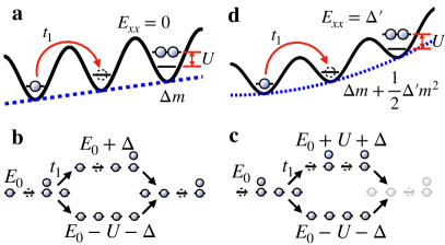
Figure 1: (a) Tensor gauge fields are absent in a linearly tilted lattice. (b) Two pathways of second-order processes give rise to the nearest neighbor tunneling of a dipole. (c) The long-range tunneling of a dipole is suppressed due to a destructive interference of two pathways. (d) A quadratic potential amounts to a finite rank-2 electric field $E_{xx}$.

We start from lineons. Since the motion of a lineon is confined in one dimension, it is sufficient to consider a one-dimensional system. As shown in Fig. 1(a), the Hamiltonian of one-dimensional bosons in a linearly tilted lattice is written as $\hat{H}_{B}=\hat{K}_{B}+\hat{V}_{B}+\sum_{m}\frac{U}{2}\hat{n}_{m}(\hat{n}_{m}-1)$, where

$$\hat{K}_{B} =-\sum_{m}(t_{1}\hat{b}^{\dagger}_{{m}}\hat{b}_{m+1}+h.c.),$$ (2)

$$\hat{V}_{B} =\sum_{m}m\Delta\hat{n}_{m},$$ (3)

and $\hat{n}_{m}=\hat{b}^{\dagger}_{{m}}\hat{b}_{{m}}$. $\Delta$ is a constant and $t_{1}$ is the single-particle tunneling strength. In the limit where $t_{1}\ll U$, double occupancy is prohibited, and each site is filled by one boson. When $t_{1}\ll\Delta$ is also satisfied, the tunneling of either the particle or the hole is suppressed. Nevertheless, a dipole can hop through some second-order processes, as shown in Fig. 1(b). These two pathways yield a finite tunneling amplitude of the dipole,

$$\hat{\tilde{K}}_{L}=-\sum_{m}(t_{2}\hat{b}^{\dagger 2}_{{m}}\hat{b}_{m+1}\hat{b}_{m-1}+h.c.),$$ (4)

where $t_{2}=-t_{1}^{2}(\frac{1}{U+\Delta}-\frac{1}{\Delta})\approx t_{1}^{2}U/\Delta^{2}$. Here, we consider the limit $U\ll\Delta$ to avoid the irrelevant tiling-assisted resonance when $U\sim\Delta$. If we define $\hat{D}_{m}^{\dagger}=\hat{b}^{\dagger}_{m}\hat{b}_{m-1}$, $\hat{\tilde{K}}_{L}=-\sum_{m}(t_{2}\hat{D}_{m}^{\dagger}\hat{D}_{m+1}+h.c.)$, describing nearest neighbor tunnelings of a dipole. Long-range tunnelings vanish due to destructive interference as shown in Fig. 1(c).

Whereas the above perturbative approach provides us with a qualitative picture, a more rigorous scheme is going to the rotating frame for eliminating the linear potential $\hat{V}_{B}$. The Hamiltonian becomes time-dependent, $\hat{\tilde{H}}_{B}=\hat{\mathcal{U}}\hat{H}\hat{\mathcal{U}}^{-1}+i\hbar(\partial_{t}\hat{\mathcal{U}})\hat{\mathcal{U}}^{-1}=\hat{\tilde{K}}_{B}(t)+\frac{U}{2}\sum_{m}\hat{n}_{m}(\hat{n}_{m}-1)$, where $\hat{\tilde{K}}_{B}=-\sum_{m}(t_{1}e^{-i\Delta t/\hbar}\hat{b}_{m}^{\dagger}b_{m+1}+h.c.)$, and

$$\hat{\mathcal{U}}=e^{i\hat{V}_{B}t/\hbar}.$$ (5)

We can then derive the Floquet Hamiltonian Goldman and Dalibard (2014),

$$\hat{\tilde{H}}_{L}=\sum_{m}\bigg{(}\frac{U}{2}-2t_{2}\bigg{)}\hat{n}_{m}(\hat{n}_{m}-1)+4t_{2}\hat{n}_{m+1}\hat{n}_{m}+\hat{\tilde{K}}_{L}.$$ (6)

Though $\hat{\tilde{H}}_{L}$ includes the kinetic energy of a lineon, $\hat{\tilde{K}}_{L}$, the lineon does not couple to a tensor gauge field. We then need to add a phase to $t_{2}$ in Eq.(4), i.e., $t_{2}\rightarrow t_{2}e^{-iA_{xx}}$. Since a constant $A_{xx}$ can be gauged away and does not lead to any physical consequence, here, we consider the simplest means to obtain a time-dependent $A_{xx}$. We add an extra small quadratic potential to the Hamiltonian, $\hat{H}_{B}^{\prime}=\hat{H}_{B}+\hat{V}_{B}^{\prime}$, where

$$\hat{V}_{B}^{\prime}=\sum_{m}\frac{1}{2}m^{2}\Delta^{\prime}\hat{n}_{m},$$ (7)

and $\Delta^{\prime}$ is a constant. To eliminate $\hat{V}_{B}+\hat{V}_{B}^{\prime}$, the unitary transformation in Eq.(5) needs to be modified,

$$\hat{\mathcal{U}}^{\prime}=e^{i(\hat{V}_{B}+\hat{V}_{B}^{\prime})t/\hbar}.$$ (8)

Using this $\hat{\mathcal{U}}^{\prime}$, $\hat{\tilde{K}}_{B}$ is replaced by $\hat{\tilde{K}}^{\prime}_{B}=-\sum_{m}(t_{1}e^{-i(\Delta+\Delta^{\prime}(m+1/2))t/\hbar}\hat{b}_{m}^{\dagger}\hat{b}_{m+1}+h.c.)$. Applying the same method, we find $\hat{\tilde{K}}_{L}$ is replaced by $\hat{\tilde{K}}^{\prime}_{L}=-\sum_{m}(t_{2}e^{-i\Delta^{\prime}t/\hbar}\hat{b}_{m}^{{\dagger}2}\hat{b}_{m+1}\hat{b}_{m-1}+h.c.)$ in the limit $\Delta\gg\Delta^{\prime}$. Compare this expression with Eq.(1), we find that $A_{xx}=\Delta^{\prime}t/\hbar$ is a rank-2 tensor gauge potential that varies linearly with time.

A time-dependent $A_{xx}$ produces a rank-2 electric field acting on dipoles,

$$E_{xx}=-\frac{\partial A_{xx}}{\partial t}=-\Delta^{\prime}/\hbar.$$ (9)

This result can also be understood from that a quadratic potential in Eq.(7) produces a linear potential for a dipole. From Eq.(7), we see that when a dipole, i.e., a particle at site $m$ and a hole at site $m-1$, move by one lattice space, the potential energy increases by a constant $\Delta^{\prime}$. A dipole thus experiences a linear potential or equivalently, a constant electric field given by Eq.(9).

We should mention that a combination of a linear potential and a quadratic one is equal to a quadratic potential that merely shifts the origin, as a well-known result. The conventional harmonic traps used in many experiments are thus able to produce $E_{xx}$. But different from ordinary experiments, the central part of the harmonic trap should be avoided. Due to the slow increase of the potential there, single-particle tunnelings cannot be suppressed. Instead, we should use the region where the gradient of the potential is strong enough to prohibit single-particle tunnelings. This can be achieved by first preparing the sample in a weak harmonic trap and then adding a strong linear potential.

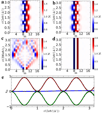
Figure 2: Time-dependent density distribution $\langle\hat{n}_{m}(t)\rangle$ of a lineon. The parameters are chosen as $U/t_{1}=4$, $\Delta/t_{1}=40$, and $\Delta^{\prime}/t_{1}=-0.01$ (a), $0.01$ (b),$0$ (c), $0.01$(d). A particle excitation is isolated from the hole in (d). These conditions lead to Bloch oscillations in opposite directions in (a) and (b), a symmetric expansion in (c) and immobile dynamics in (d). (e)$x_{D}$ as a function of time. Results of the exact diagonalization of the effective Hamiltonian of a single dipole are shown in red dotted (a), green dashed (b) and blue dash-dotted lines (c). Black curves are results of the full Hamiltonians using TEBD. Horizontal lines denote $-4t_{2}/\Delta^{\prime}$.

To explicitly show the effect of $E_{xx}$, we have numerically computed the dynamics of a lineon using the time-evolution block-decimation (TEBD) method. The Hamiltonian is chosen as $\hat{H}_{B}^{\prime}$ which includes both a strong linear potential and a weak quadratic potential. The initial state includes a single dipole, i.e., a single particle-hole excitation in a Mott insulator. Whereas the initial state of the dipole can be an arbitrary wavepacket, for convenience, we let the superposition state of the dipole occupy two lattice sites, i.e., $\ket{\Psi(t=0)}=(\hat{D}^{\dagger}_{0}+\hat{D}^{\dagger}_{1})|\text{MI}\rangle/2$, where $|\text{MI}\rangle=\prod_{m}\hat{b}^{\dagger}_{m}|0\rangle$ is a Mott insulator with one particle per site. As shown in Fig. 2(a-c), when $\Delta^{\prime}=0$, the wavepacket simply expands symmetrically towards both directions as $t$ increases. Once $\Delta^{\prime}\neq 0$, the wavepacket moves towards one direction as a result of a finite $E_{xx}$. Changing the sign of $\Delta^{\prime}$ reverses the direction of the motion. In contrast, if the separation between the particle and the hole is larger than one lattice spacing, each of them becomes an isolated excitation. Neither the particle nor the hole moves, as shown in Fig. 2(d).

To further quantitatively characterize the dynamics of a dipole, we define

$${x}_{D}=\frac{1}{2}\langle\sum_{m=1}^{L}[m-(L{+}1)/2]^{2}\hat{n}_{m}\rangle-\frac{1}{24}L(L^{2}-1).$$ (10)

In the absence of a dipole, $\langle\hat{n}_{m}\rangle=1$, $x_{D}=0$. When there is an additional particle at site $m+1$ and a hole at site $m$, $x_{D}=m-L/2$. We therefore read from ${x}_{D}$ the position of the dipole. From Fig. 2(e), it is clear that $x_{D}$ oscillates as time goes by when $\Delta^{\prime}\neq 0$. We have smoothed the curves by averaging the results within a much smaller time scale $2\pi\hbar/\Delta$ (Supplementary Materials). In the presence of a finite $E_{xx}=-\Delta^{\prime}/\hbar$, the energy penalty for a dipole to hop to the nearest neighbor site is $\hbar E_{xx}$. The effective Hamiltonian of a single dipole is written as $\hat{H}_{\rm eff}=\hat{\tilde{K}}_{L}-\hbar E_{xx}\sum_{m}m\hat{D}^{\dagger}_{m}\hat{D}_{m}{/2}$. The period of the Bloch oscillation of a dipole is given by $T_{D}=2\pi/|E_{xx}|$. Using Eq.(9), we obtain

$$T_{D}=2\pi\frac{\hbar}{|\Delta^{\prime}|}.$$ (11)

The results of $H_{\rm eff}$ are shown in Fig.2(e). Similarly, the oscillation amplitude is given by $-4t_{2}/\Delta^{\prime}$ (Supplementary material). Both expressions agree well with the numerical solution of the full Hamiltonian of bosons $\hat{H}^{\prime}_{B}$ using TEBD.

As for vector gauge fields, though a linear external potential in the real space is equivalent to a time-dependent vector potential, it is useful to realize the latter directly in experiments. The same consideration applies to tensor gauge fields. To this end, we consider another method of using external lasers to induce photon-assisted tunnelings. Such tunnelings naturally carry the phases of external lasers and can be made position-dependent, as shown in Fig. 3. This scheme was used in pioneering works of realizing the Harper-Hofstadter model Aidelsburger et al. (2013); Miyake et al. (2013). Here, a key difference is that, instead of using a resonant coupling, we consider a finite detuning, $\Delta=\Delta_{0}-\hbar\omega$, where $\Delta_{0}$ is the energy mismatch between the nearest neighbor sites of the linearly tilted lattice, and $\omega$ is the frequency of the driving field. If one uses Raman lasers, $\omega=\omega_{1}-\omega_{2}$ will be the difference between the frequencies of the two lasers. As such, there exists a residual linear potential described by Eq.(3). The one-dimensional system is then described by the same Hamiltonian described before. Most of the remaining discussions apply except an important difference that $\hat{K}_{B}$ is replaced by

$$\hat{K}^{\prime}_{B}=-\sum_{m}(t_{1}e^{-im\theta}\hat{b}^{\dagger}_{{m}}\hat{b}_{m+1}+h.c.).$$ (12)

Correspondingly, the difference in the phase carried by the particle and the hole leads to a finite phase in the tunneling of a dipole. The kinetic energy of a dipole is then readily given by Eq.(1), where $A_{xx}=\theta$, and there is no need to introduce an extra quadratic potential. To have a time-dependent $A_{xx}$, we recall that $\theta=({\bf k}_{1}-{\bf k}_{2})\cdot\bf{a}$, where ${\bf k}_{i=1,2}$ is the wave vectors of the Raman lasers and ${\bf a}$ is the unit vector of the lattice. The incident angles of the Raman lasers can then be changed as time goes by.

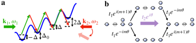
Figure 3: (a) Raman lasers (green and red arrows) produce photon-assisted tunnelings in a linearly tilted lattice. A finite detuning $\Delta=\Delta_{0}-\hbar\omega$ leads to a residual linear potential. (b) The site-dependent phase of the single-particle tunneling provides a phase in the tunneling of a dipole (violet arrow).

In higher dimensions, physics becomes even richer. Whereas the previously discussed method still works for lineons, there exist planons that could move in two directions that are perpendicular to the dipole moment. To simplify notations, we consider two dimensions as an example. A ring-exchange interaction allows a planon to move,

$$\hat{\tilde{K}}_{P}=-\sum_{\bf m}(t_{2}^{\prime}\hat{b}^{\dagger}_{\bf m}\hat{b}^{\dagger}_{{\bf m}+\hat{\bf x}+\hat{\bf y}}\hat{b}_{{\bf m}+\hat{\bf x}}\hat{b}_{{\bf m}+\hat{\bf y}}+h.c.),$$ (13)

where ${\bf m}=(m_{x},m_{y})$ is the lattice index and $\hat{\bf x}$ and $\hat{\bf y}$ are the unit vectors in the $x$ and $y$ directions, respectively. If we define the creation operator for a planon as $\hat{D}^{\dagger}_{{\bf m},{\bf\hat{n}}}=\hat{b}^{\dagger}_{\bf m}\hat{b}_{{\bf m}-\hat{\bf n}}$, where $\hat{\bf n}=\hat{\bf x},\hat{\bf y}$, $t_{2}^{\prime}$ corresponds to the tunneling strength of a planon. When applying similar second-order processes of single-particle tunnelings as that in discussions about lineons, it produces both the ring-exchange interaction and kinetic energies of lineons (Supplementary Materials).

To access purely a ring-exchange interaction with a controllable phase, we consider an alternative scheme using particles with long-range interactions in a lattice. As shown in Fig. 4(a), the lattice potential in the $x$ direction is strong such that the tunneling along this direction is suppressed, i.e., $t_{x}=0$. In the $y$ direction, Raman lasers imprint a $x$-dependent phase in the tunneling, $t_{y}e^{im_{x}\theta}$. The Hamiltonian is written as $\hat{H}_{M}=\hat{K}_{M}+\hat{U}_{M}$, where

$$\hat{K}_{M} =-\sum_{\bf m}(t_{y}e^{im_{x}\theta}\hat{b}^{\dagger}_{\bf m}\hat{b}_{{\bf m}+\hat{\bf y}}+h.c.),$$ (14)

$$\hat{U}_{M} =\frac{U}{2}\sum_{\bf m}\hat{n}_{\bf m}(\hat{n}_{\bf m}-1)+V\sum_{\langle{\bf m},{\bf n}\rangle}\hat{n}_{\bf m}\hat{n}_{\bf n}.$$ (15)

$V$ denotes the nearest neighbor interaction. Here, we consider an isotropic nearest-neighbor interaction for simplicity. Anisotropic interactions do not change the main results.

When a dipole is aligned along the $x$ direction, the tunneling of either the particle or the hole is suppressed in the limit where $V\gg t_{y}$, as such tunnelings lead to an extra energy penalty, as shown in Fig. 4(a). Nevertheless, second-order processes allow such a dipole to tunnel in the $y$ direction. The kinetic energy of this planon is written as

$$\hat{K}_{P}=-\sum_{\bf m}(J_{y}e^{-iA_{xy}}\hat{D}^{\dagger}_{\bf m,\hat{\bf x}}\hat{D}_{{\bf m}+\hat{\bf y},\hat{\bf x}}+h.c.),$$ (16)

where $J_{y}=-2t_{y}^{2}/V$, and $A_{xy}=\theta$ denotes a synthetic tensor gauge field. Similar to previous discussions, a time-dependent $A_{xy}$ gives rise to an electric field $E_{xy}=-\partial\theta/\partial t$ acting on a planon. This time, planon will perform Bloch oscillations in the direction perpendicular to the dipole moment.

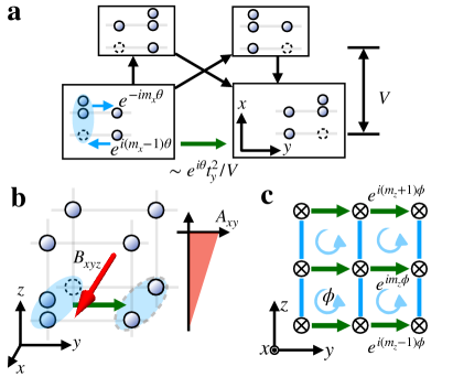
Figure 4: (a) The tunneling of a planon (green thick arrow) through second-order processes of single-particle tunnelings (thin black arrow). (b) A $z$-dependent $A_{xy}$ provides a magnetic field for the planon. (c) The side view of (b) represents a dipolar Harper-Hofstadter model where each plaquette is threaded with a finite flux $\phi$.

Going to three dimensions, the variance of $A_{xy}$ in the $z$ direction leads to a magnetic field $B_{xyz}=-\partial A_{xy}/\partial z$. As shown in Fig. 4(b), such a magnetic field can be accessed by introducing a $z$-dependent $\theta=\phi z$. To this end, we consider a three-dimensional model, $\hat{H}^{\prime}_{M}=\hat{K}^{\prime}_{M}+\hat{U}_{M}$, where

$$\hat{K}^{\prime}_{M}=-\sum_{\bf m}(t_{y}e^{im_{x}m_{z}\phi}\hat{b}^{\dagger}_{\bf m}\hat{b}_{{\bf m}+\hat{\bf y}}+t_{z}\hat{b}^{\dagger}_{\bf m}\hat{b}_{{\bf m}+\hat{\bf z}}+h.c.).$$ (17)

$\hat{m}=(m_{x},m_{y},m_{z})$ has been promoted to the index of a three-dimensional lattice. For a fixed $m_{x}$, the phase carried by $t_{y}$ changes linearly as a function of $m_{z}$. We thus just need to generalize the scheme of realizing the Harper-Hofstadter model to a $m_{x}$ dependent one. The simplest scheme is to use the synthetic dimension formed by internal degrees of freedom like hyperfine spins or different atomic species, which may feel different vector gauge potentials Aidelsburger et al. (2013). As the tunneling in the $x$ direction is suppressed, it is sufficient to consider only two layers with $m_{x}=0$ and $m_{x}=1$, respectively. In other words, only a two-component system is required. Applying component-selective Raman lasers that do not affect the first component, the tunneling of this component is unchanged. $t_{y}$ in the first layer with $m_{x}=0$ thus does not acquire an additional phase. In contrast, the Raman lasers imprint a phase to the tunneling of the second component. $t_{y}$ in the second layer with $m_{x}=1$ thus becomes $t_{y}e^{im_{z}\phi}$. The minimal version of Eq.(17) is then realized. Alternatively, if one directly implements the scheme in Aidelsburger et al. (2013), where these two components feel opposite vector gauge potentials, $\phi\rightarrow 2\phi$.

Once accessing Eq.(17) in laboratories, a dipolar Harper-Hofstadter model is realizable. Similar to the previous discussions, a dipole aligned in the $x$ direction can also tunnel in the $z$ direction with a tunneling strength $J_{z}=-t_{z}^{2}/V$. If we view the system along the $x$-axis, the dipole appears to be a two-dimensional particle moving in the $y-z$ plane, as shown in Fig. 4(c). This thus realizes a dipolar Harper-Hofstadter model,

$$\begin{split}\hat{H}_{\rm dHH}=&\frac{1}{2}\sum_{\bf m}(J_{y}e^{-im_{z}\phi}\hat{D}_{\bf m,\hat{x}}\hat{D}^{\dagger}_{\bf m+\hat{y},\hat{x}}\\ &+J_{z}\hat{D}_{\bf m,\hat{x}}\hat{D}^{\dagger}_{\bf m+\hat{z},\hat{x}}+h.c.).\end{split}$$ (18)

where the flux included in a single plaquette becomes finite. This dipolar Harper-Hofstadter model is expected to host many new quantum phenomena. Unlike conventional Chern insulators, the edge of a finite strip of such a model features a vanishing particle current but a finite dipole current that is worth future theoretical and experimental studies.

We have shown that some simple protocols fulfill the lofty goal of creating synthetic tensor gauge fields in laboratories. Our scheme can be generalized to fermions and multi-component systems. It is also possible to realize even higher rank gauge fields using related schemes. We hope that our work may stimulate more interest to study higher rank gauge fields.

This work is supported by the U.S. Department of Energy, Office of Science through the Quantum Science Center (QSC), a National Quantum Information Science Research Center and National Science Foundation (NSF) through Grant No. PHY-2110614. S.Zhang is supported by National Natural Science Foundation of China(Grant No.12174138).

Supplementary Materials for

“Synthetic tensor gauge fields”

In this supplementary material, we present results of the fast oscillation due to the micromotion of single particles, the amplitude of Bloch oscillation, and a scheme that produces both the ring-exchange interaction and the kinetics of lineons.

.1 Fast oscillations due to the micromotion of single-particles

When deriving the effective Hamiltonian for the dipole using the Floquet theory, we have dropped off the micromotion of single-particles. In the presence of a strong linear potential, a single particle experiences a Bloch oscillation with a frequency $\omega_{s}=\Delta/\hbar$. This is a micromotion in a much smaller time scale than that of the Bloch oscillation of the dipole. Whereas numerical results clearly show such fast oscillations, we consider the average over time in such a small scale $T_{f}=2\pi/\omega_{s}$ to smooth the results. Here, we show similar numerical results as that in Fig. 2 (e) using exact diagonalization with $L=7$. The main figure in Fig. S1(a) show the result before doing the average. The fast oscillations are highlighted in the inset. Fig. S1(b) shows the result after doing the average.

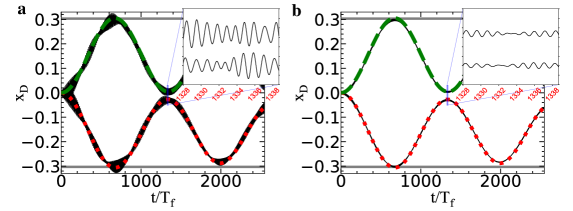
Figure S1: $x_{D}$ as a function of the time before (a) and after (b) averaging over a small time period $T_{f}=2\pi\hbar/\Delta$. The parameters are chosen as $U/t_{1}=4$, $\Delta/t_{1}=40$ and $\Delta^{\prime}/t_{1}=-0.03$, $0.03$. Results of the exact diagonalization of the effective Hamiltonian of a single dipole are shown in red dotted ($\Delta^{\prime}/t_{1}=0.03$), green dashed ($\Delta^{\prime}/t_{1}=-0.03$) lines. Black curves are the results of the exact diagonalization of the full Hamiltonians. Horizontal lines denote $-4t_{2}/\Delta^{\prime}$. Insets show the results in a small time window.

.2 The amplitude of Bloch oscillation

Within the effective theory, the dipole dynamics is captured by a tight-binding Hamiltonian with a linear potential,

$$\hat{H}_{\rm eff}=\sum_{m}-2t_{2}(\ket{m}\bra{m+1}+h.c.)+\Delta^{\prime}m\ket{m}\bra{m},$$ (S1)

where $\ket{m}=\hat{D}^{\dagger}_{m}\ket{\rm MI}/\sqrt{2}$ denotes the normalized single dipole state. The eigenstates of the effective Hamiltonian $\hat{H}_{\rm eff}$ are the Wannier Stark states. The time evolution operator is written as Hartmann et al. (2004)

$$U(t)=\sum_{m,m^{\prime}}J_{m-m^{\prime}}(8t_{2}\sin(\Delta^{\prime}t/2\hbar)/\Delta^{\prime})e^{i(m-m^{\prime})(\pi-\Delta^{\prime}t/\hbar)/2-im^{\prime}\Delta^{\prime}t/\hbar}\ket{m}\bra{m^{\prime}},$$ (S2)

where $J_{m}(x)$ is the Bessel function of the first kind. $U(t)$ has a period $T=2\pi\hbar/\Delta^{\prime}$. Without loss of generality, we consider an initial state $\ket{\psi(0)}=(\ket{0}+\ket{1})/\sqrt{2}$. The quantum state reaches its maximal extension at half of the oscillation period. The averaged dipole displacement corresponding to the oscillation amplitude is written as

$$\bra{\psi(T/2)}m\ket{\psi(T/2)}-\bra{\psi(0)}m\ket{\psi(0)}=\sum_{m}\frac{1}{2}\bigg{(}J_{m}(8t_{2}/\Delta^{\prime})-J_{m-1}(8t_{2}/\Delta^{\prime})\bigg{)}^{2}m-\frac{1}{2}=-\frac{4t_{2}}{\Delta^{\prime}}.$$ (S3)

.3 Producing both the ring-exchange interaction and kinetics of lineons

We consider a two-dimensional Hamiltonian that is written as $\hat{H}_{B}=\hat{K}_{B}+\hat{V}_{B}+\hat{U}_{B}$ where

$$\begin{aligned} \hat{K}_{B}=&-\sum_{{\bf m},\hat{\bf n}}(t_{1}\hat{b}_{\bf m}\hat{b}_{{\bf m}+\hat{\bf n}}+h.c.),\\ \hat{V}_{B}=&\sum_{\bf m}(m_{x}\Delta_{x}+m_{y}\Delta_{y})\hat{n}_{\bf m},\\ \hat{U}_{B}=&\frac{U}{2}\sum_{\bf m}\hat{n}_{\bf m}(\hat{n}_{\bf m}-1)+V\sum_{\bf m}\hat{n}_{\bf m}(\hat{n}_{\bf m+\hat{x}}+\hat{n}_{\bf m+\hat{y}}).\end{aligned}$$ (S4)

$\Delta_{x}$ and $\Delta_{y}$ are energy mismatches between nearest-neighbor sites along the $x$ and $y$ directions, respectively. In 2D, the finite nearest-neighbor interaction $V$ is necessary for realizing correlated pair tunnelings through second-order processes of single-particle tunnelings. Such $V$ can be realized by using polar molecules or Rydberg atom arrays. As shown by Fig.S2, when $V\neq 0$, four pathways yield a finite amplitude of the ring-exchange interaction, allowing a planon to tunnel along the perpendicular direction of the dipole moment,

$$\hat{\tilde{K}}_{P}=-\sum_{\bf m}(t_{2}^{\prime}\hat{b}^{\dagger}_{\bf m}\hat{b}^{\dagger}_{{\bf m}+\hat{\bf x}+\hat{\bf y}}\hat{b}_{{\bf m}+\hat{\bf x}}\hat{b}_{{\bf m}+\hat{\bf y}}+h.c.),$$ (S5)

where $t^{\prime}_{2}=t^{\prime}_{2x}+t^{\prime}_{2y}$ and $t^{\prime}_{2x}=\frac{2V}{V^{2}-\Delta^{2}_{x}}t^{2}_{1}$, $t^{\prime}_{2y}=\frac{2V}{V^{2}-(U+\Delta_{y})^{2}}t^{2}_{1}$.

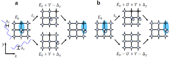
Figure S2: The ring-exchange interaction. (a) and (b) correspond to the second-order processes of single-particle tunnelings along the $x$ and the $y$ directions, respectively.

Some other tunnelings of a dipole can also be produced by second-order processes, as shown in Fig.S3. For example, the tunneling of a lineon exists,

$$\hat{\tilde{K}}_{L}=-\sum_{\bf m}(t_{2}\hat{b}^{{\dagger}2}_{\bf m}\hat{b}_{\bf m+\hat{y}}\hat{b}_{\bf m-\hat{y}}+\tilde{t}_{2}\hat{b}^{\dagger}_{\bf m-\hat{y}}\hat{b}^{\dagger}_{\bf m}\hat{b}_{\bf m+\hat{y}}\hat{b}_{\bf m+2\hat{y}}+h.c.),$$ (S6)

where $t_{2}=\frac{(2V-U)}{(V+\Delta_{y})(V-U-\Delta_{y})}t^{2}_{1}$ and $\tilde{t}_{2}=\frac{V}{(U-2V+\Delta_{y})(U-V+\Delta_{y})}t^{2}_{1}$ correspond to the amplitude of the nearest-neighbor and the next-nearest-neighbor tunneling of a lineon, respectively. Furthermore, the dipole can tunnel along the diagonal direction,

$$\hat{\tilde{K}}_{\mathrm{diag}}=-\sum_{\bf m}(\tilde{t}_{\hat{x}+\hat{y}}\hat{b}^{\dagger}_{\bf m}\hat{b}_{\bf m+\hat{y}}\hat{b}_{\bf m+\hat{x}+\hat{y}}\hat{b}^{\dagger}_{\bf m+\hat{x}+2\hat{y}}+\tilde{t}_{\hat{x}-\hat{y}}\hat{b}^{\dagger}_{\bf m}\hat{b}_{\bf m+\hat{y}}\hat{b}_{\bf m+\hat{x}-\hat{y}}\hat{b}^{\dagger}_{\bf m+\hat{x}}+h.c.),$$ (S7)

where $\tilde{t}_{\hat{x}+\hat{y}}=\tilde{t}_{\hat{x}+\hat{y}}=\tilde{t}_{2}$.

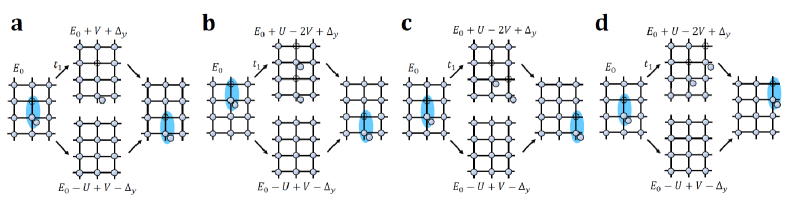
Figure S3: (a) and (b) depict the nearest-neighbor and next-nearest-neighbor hopping of a lineon, respectively. (c) and (d) depict the tunnelings of a dipole along the diagonal directions.

We define $\hat{D}^{\dagger}_{\bf m,\hat{\bf y}}=\hat{b}^{\dagger}_{\bf m}\hat{b}_{\bf m-\hat{y}}$, the creation operator of a dipole along the $y$ direction. The kinetic energy of the dipole can be written as

$$\begin{aligned} \hat{\tilde{K}}_{D}&=-\sum_{\bf m}\big{\{}t^{\prime}_{2}\hat{D}^{\dagger}_{{\bf m+\hat{x}},\hat{\bf y}}\hat{D}_{{\bf m},\hat{\bf y}}+t_{2}\hat{D}^{\dagger}_{{\bf m+\hat{y}},\hat{\bf y}}\hat{D}_{{\bf m},\hat{\bf y}}\\ &+\tilde{t}_{2}(\hat{D}^{\dagger}_{{\bf m+2\hat{x}},\hat{\bf y}}+\hat{D}^{\dagger}_{{\bf m+\hat{x}+\hat{y}},\hat{\bf y}}+\hat{D}^{\dagger}_{{\bf m+\hat{x}-\hat{y}},\hat{\bf y}})\hat{D}_{{\bf m},\hat{\bf y}}+h.c.\big{\}}\end{aligned}$$ (S8)

We note that, in the limit where $U$ is much larger than any other energy scales, $t^{\prime}_{2}\rightarrow\frac{2V}{V^{2}-\Delta^{2}_{x}}t_{1}^{2}$, $t_{2}\rightarrow\frac{1}{V+\Delta_{y}}t_{1}^{2}$, and $\tilde{t}_{2}\rightarrow 0$. In this limit, only the nearest neighbor tunnelings exist but a dipole can tunnel in both directions, being a superposition of a lineon and a planon.

To create a tensor gauge field, similar to discussions in the main text, an extra small quadratic potential in the $x-y$ plane can be added, $\hat{H}^{\prime}_{B}=\hat{H}_{B}+\hat{V}_{L}$ where

$$\hat{V}^{\prime}_{B}=\frac{1}{2}\sum_{\bf m}(\alpha m_{x}+\beta m_{y})^{2}\Delta^{\prime}\hat{n}_{\bf m},$$ (S9)

where $\alpha$ and $\beta$ are both dimensionless coefficients to control the direction of quadratic potential satisfying $\alpha^{2}+\beta^{2}=1$. Using a unitary transformation to eliminate $\hat{V}_{B}+\hat{V}^{\prime}_{B}$, the single-particle tunneling acquires an additional time-dependent phase,

$$\begin{aligned} \hat{\tilde{K}}_{B}=&-\sum_{\bf m}(t_{1}e^{-i\Delta_{x}t-i(m_{x}+1/2)\alpha^{2}\Delta^{\prime}t-im_{y}\alpha\beta\Delta^{\prime}t}\hat{b}^{\dagger}_{\bf m}\hat{b}_{\bf m+\hat{x}}\\ &+t_{1}e^{-i\Delta_{y}t-im_{x}\alpha\beta\Delta^{\prime}t-i(m_{y}+1/2)\beta^{2}\Delta^{\prime}t}\hat{b}^{\dagger}_{\bf m}\hat{b}_{\bf m+\hat{y}}+h.c.)\end{aligned}$$ (S10)

In the limit $\Delta^{\prime}\ll\Delta$, the Floquet theory gives rise to a ring-exchange interaction,

$$\hat{\tilde{K}}_{P}=-\sum_{\bf m}(t_{2}^{\prime}e^{-i\alpha\beta\Delta^{\prime}t}\hat{b}^{\dagger}_{\bf m}\hat{b}^{\dagger}_{{\bf m}+\hat{\bf x}+\hat{\bf y}}\hat{b}_{{\bf m}+\hat{\bf x}}\hat{b}_{{\bf m}+\hat{\bf y}}+h.c.).$$ (S11)

Similar discussions apply to other tunnelings.

References

- Lasenby et al. (1998) A. Lasenby, C. Doran, and S. Gull, Gravity, gauge theories and geometric algebra, Philosophical Transactions of the Royal Society of London. Series A: Mathematical, Physical and Engineering Sciences 356, 487 (1998).
- Thouless et al. (1982) D. J. Thouless, M. Kohmoto, M. P. Nightingale, and M. den Nijs, Quantized Hall conductance in a two-dimensional periodic potential, Phys. Rev. Lett. 49, 405 (1982).
- Tsui et al. (1982) D. C. Tsui, H. L. Stormer, and A. C. Gossard, Two-dimensional magnetotransport in the extreme quantum limit, Phys. Rev. Lett. 48, 1559 (1982).
- König et al. (2007) M. König, S. Wiedmann, C. Brüne, A. Roth, H. Buhmann, L. W. Molenkamp, X.-L. Qi, and S.-C. Zhang, Quantum spin Hall insulator state in HgTe quantum wells, Science 318, 766 (2007).
- Lin et al. (2011) Y.-J. Lin, R. L. Compton, K. Jiménez-García, W. D. Phillips, J. V. Porto, and I. B. Spielman, A synthetic electric force acting on neutral atoms, Nature Physics 7, 531 (2011).
- Aidelsburger et al. (2011) M. Aidelsburger, M. Atala, S. Nascimbène, S. Trotzky, Y.-A. Chen, and I. Bloch, Experimental realization of strong effective magnetic fields in an optical lattice, Phys. Rev. Lett. 107, 255301 (2011).
- Aidelsburger et al. (2013) M. Aidelsburger, M. Atala, M. Lohse, J. T. Barreiro, B. Paredes, and I. Bloch, Realization of the Hofstadter Hamiltonian with ultracold atoms in optical lattices, Phys. Rev. Lett. 111, 185301 (2013).
- Miyake et al. (2013) H. Miyake, G. A. Siviloglou, C. J. Kennedy, W. C. Burton, and W. Ketterle, Realizing the Harper Hamiltonian with laser-assisted tunneling in optical lattices, Phys. Rev. Lett. 111, 185302 (2013).
- Schweizer et al. (2019) C. Schweizer, F. Grusdt, M. Berngruber, L. Barbiero, E. Demler, N. Goldman, I. Bloch, and M. Aidelsburger, Floquet approach to lattice gauge theories with ultracold atoms in optical lattices, Nature Physics 15, 1168 (2019).
- Görg et al. (2019) F. Görg, K. Sandholzer, J. Minguzzi, R. Desbuquois, M. Messer, and T. Esslinger, Realization of density-dependent Peierls phases to engineer quantized gauge fields coupled to ultracold matter, Nature Physics 15, 1161 (2019).
- Yang et al. (2020) B. Yang, H. Sun, R. Ott, H.-Y. Wang, T. V. Zache, J. C. Halimeh, Z.-S. Yuan, P. Hauke, and J.-W. Pan, Observation of gauge invariance in a 71-site Bose–Hubbard quantum simulator, Nature 587, 392 (2020).
- Li et al. (2022) C.-H. Li, Y. Yan, S.-W. Feng, S. Choudhury, D. B. Blasing, Q. Zhou, and Y. P. Chen, Bose-Einstein condensate on a synthetic topological Hall cylinder, PRX Quantum 3, 010316 (2022).
- Zhou et al. (2022) Z.-Y. Zhou, G.-X. Su, J. C. Halimeh, R. Ott, H. Sun, P. Hauke, B. Yang, Z.-S. Yuan, J. Berges, and J.-W. Pan, Thermalization dynamics of a gauge theory on a quantum simulator, Science 377, 311 (2022).
- Hafezi et al. (2011) M. Hafezi, E. A. Demler, M. D. Lukin, and J. M. Taylor, Robust optical delay lines with topological protection, Nature Physics 7, 907 (2011).
- Khanikaev et al. (2013) A. B. Khanikaev, S. Hossein Mousavi, W.-K. Tse, M. Kargarian, A. H. MacDonald, and G. Shvets, Photonic topological insulators, Nature Materials 12, 233 (2013).
- Mittal et al. (2014) S. Mittal, J. Fan, S. Faez, A. Migdall, J. M. Taylor, and M. Hafezi, Topologically robust transport of photons in a synthetic gauge field, Phys. Rev. Lett. 113, 087403 (2014).
- Süsstrunk and Huber (2015) R. Süsstrunk and S. D. Huber, Observation of phononic helical edge states in a mechanical topological insulator, Science 349, 47 (2015).
- Xiao et al. (2015) M. Xiao, W.-J. Chen, W.-Y. He, and C. T. Chan, Synthetic gauge flux and Weyl points in acoustic systems, Nature Physics 11, 920 (2015).
- Lee et al. (2018) C. H. Lee, S. Imhof, C. Berger, F. Bayer, J. Brehm, L. W. Molenkamp, T. Kiessling, and R. Thomale, Topolectrical circuits, Communications Physics 1 (2018), 10.1038/s42005-018-0035-2.
- Boada et al. (2012) O. Boada, A. Celi, J. I. Latorre, and M. Lewenstein, Quantum simulation of an extra dimension, Phys. Rev. Lett. 108, 133001 (2012).
- Celi et al. (2014) A. Celi, P. Massignan, J. Ruseckas, N. Goldman, I. B. Spielman, G. Juzeliūnas, and M. Lewenstein, Synthetic gauge fields in synthetic dimensions, Phys. Rev. Lett. 112, 043001 (2014).
- An et al. (2017) F. A. An, E. J. Meier, and B. Gadway, Direct observation of chiral currents and magnetic reflection in atomic flux lattices, Science Advances 3 (2017), 10.1126/sciadv.1602685.
- Lustig et al. (2019) E. Lustig, S. Weimann, Y. Plotnik, Y. Lumer, M. A. Bandres, A. Szameit, and M. Segev, Photonic topological insulator in synthetic dimensions, Nature 567, 356 (2019).
- Cui et al. (2013) X. Cui, B. Lian, T.-L. Ho, B. L. Lev, and H. Zhai, Synthetic gauge field with highly magnetic Lanthanide atoms, Phys. Rev. A 88, 011601 (2013).
- Palumbo et al. (2018) G. Palumbo, and N. Goldman, Revealing Tensor Monopoles through Quantum-Metric Measurements, Phys. Rev. Lett. 121, 170401 (2018).
- Chen et al. (2022) M. Chen, C. Li, G. Palumbo, Y.-Q. Zhu, N. Goldman, and P. Cappellaro, A synthetic monopole source of Kalb-Ramond field in diamond, Science 375, 1017-1020 (2022).
- Tan et al. (2021) X. Tan, D.-W. Zhang, W. Zheng, X. Yang, S. Song, Z. Han, Y. Dong, Z. Wang, D. Lan, H. Yan, S.-L. Zhu, and Y. Yu, Experimental Observation of Tensor Monopoles with a Superconducting Qudit, Phys. Rev. Lett. 126, 017702 (2021).
- Zhu et al. (2020) Y.-Q. Zhu, N. Goldman, and G. Palumbo, Four-dimensional semimetals with tensor monopoles: From surface states to topological responses, Phys. Rev. B 102, 081109 (2020).
- Chamon (2005) C. Chamon, Quantum glassiness in strongly correlated clean systems: An example of topological overprotection, Phys. Rev. Lett. 94, 040402 (2005).
- Bravyi et al. (2011) S. Bravyi, B. Leemhuis, and B. M. Terhal, Topological order in an exactly solvable 3D spin model, Annals of Physics 326, 839 (2011).
- Haah (2011) J. Haah, Local stabilizer codes in three dimensions without string logical operators, Phys. Rev. A 83, 042330 (2011).
- Yoshida (2013) B. Yoshida, Exotic topological order in fractal spin liquids, Phys. Rev. B 88, 125122 (2013).
- Vijay et al. (2015) S. Vijay, J. Haah, and L. Fu, A new kind of topological quantum order: A dimensional hierarchy of quasiparticles built from stationary excitations, Phys. Rev. B 92, 235136 (2015).
- Vijay et al. (2016) S. Vijay, J. Haah, and L. Fu, Fracton topological order, generalized lattice gauge theory, and duality, Phys. Rev. B 94, 235157 (2016).
- Pretko (2017a) M. Pretko, Subdimensional particle structure of higher rank spin liquids, Phys. Rev. B 95, 115139 (2017a).
- Pretko (2017b) M. Pretko, Generalized electromagnetism of subdimensional particles: A spin liquid story, Phys. Rev. B 96, 035119 (2017b).
- Nandkishore and Hermele (2019) R. M. Nandkishore and M. Hermele, Fractons, Annual Review of Condensed Matter Physics 10, 295 (2019).
- Pretko et al. (2020) M. Pretko, X. Chen, and Y. You, Fracton phases of matter, International Journal of Modern Physics A 35, 2030003 (2020).
- Scherg et al. (2021) S. Scherg, T. Kohlert, P. Sala, F. Pollmann, B. H. Madhusudhana, I. Bloch, and M. Aidelsburger, Observing non-ergodicity due to kinetic constraints in tilted Fermi-Hubbard chains, Nature Communications 12 (2021), 10.1038/s41467-021-24726-0.
- Lake et al. (2022) E. Lake, M. Hermele, and T. Senthil, Dipolar Bose-Hubbard model, Phys. Rev. B 106, 064511 (2022).
- Lake et al. (2023) E. Lake, H.-Y. Lee, J. H. Han, and T. Senthil, Dipole condensates in tilted Bose-Hubbard chains, Phys. Rev. B 107, 195132 (2023).
- Kohlert et al. (2023) T. Kohlert, S. Scherg, P. Sala, F. Pollmann, B. Hebbe Madhusudhana, I. Bloch, and M. Aidelsburger, Exploring the regime of fragmentation in strongly tilted Fermi-Hubbard chains, Phys. Rev. Lett. 130, 010201 (2023).
- Pretko (2017c) M. Pretko, Emergent gravity of fractons: Mach’s principle revisited, Phys. Rev. D 96, 024051 (2017c).
- Pai and Pretko (2018) S. Pai and M. Pretko, Fractonic line excitations: An inroad from three-dimensional elasticity theory, Phys. Rev. B 97, 235102 (2018).
- Ma et al. (2018) H. Ma, M. Hermele, and X. Chen, Fracton topological order from the Higgs and partial-confinement mechanisms of rank-two gauge theory, Phys. Rev. B 98, 035111 (2018).
- Bulmash and Barkeshli (2018) D. Bulmash and M. Barkeshli, Higgs mechanism in higher-rank symmetric U(1) gauge theories, Phys. Rev. B 97, 235112 (2018).
- Goldman and Dalibard (2014) N. Goldman and J. Dalibard, Periodically driven quantum systems: Effective Hamiltonians and engineered gauge fields, Phys. Rev. X 4, 031027 (2014).

References

- Hartmann et al. (2004) T. Hartmann, F. Keck, H. J. Korsch, and S. Mossmann, Dynamics of Bloch oscillations, New Journal of Physics 6, 2 (2004).