Abstract

Comparing and evaluating small area estimation (SAE) models for a given application is inherently difficult. Typically, we do not have enough data in many areas to check unit-level modeling assumptions or to assess unit-level predictions empirically; and there is no ground truth available for checking area-level estimates. Design-based simulation from artificial populations can help with each of these issues, but only if the artificial populations (a) realistically represent the application at hand and (b) are not built using assumptions that could inherently favor one SAE model over another. In this paper, we borrow ideas from random hot deck, approximate Bayesian bootstrap (ABB), and $k$ nearest neighbor (kNN) imputation methods, which are often used for multiple imputation of missing data. We propose a kNN-based approximation to ABB (KBAABB) for a different purpose: generating an artificial population when rich unit-level auxiliary data is available. We introduce diagnostic checks on the process of building the artificial population itself, and we demonstrate how to use such an artificial population for design-based simulation studies to compare and evaluate SAE models, using real data from the Forest Inventory and Analysis (FIA) program of the US Forest Service. We illustrate how such simulation studies may be disseminated and explored interactively through an online R Shiny application.

1 Introduction

The USDA 2014 and 2018 Farm Bills [1, 2] direct the Forest Inventory and Analysis (FIA) Program to: “implement procedures to improve the statistical precision of estimates at the sub-State level” and “find efficiencies in the operations of the Forest Inventory and Analysis Program under section 3(e) of the Forest and Rangeland Renewable Resources Research Act of 1978 (16 U.S.C. 1642(e)) through the improved use and integration of advanced remote sensing technologies to provide estimates for State- and national-level inventories, where appropriate.” The FIA program (https://www.fia.fs.fed.us/) provides data and tools for delivering standardized estimates at state levels over 5-10 year periods, but there is currently no standardized methodology to generate estimates at these sub-State levels or shorter time intervals. The need for more precise information of ecological characteristics and integrity at sub-State levels is essential for field specialists and managers to make tactical assessments for local and broad-scale monitoring and planning. In response to the Farm Bill initiatives, FIA is working towards a strategic plan to define FIA user needs, evaluate small area estimation (SAE) methodology, and deliver statistically sound, standardized estimates to users at the sub-State level.

Estimation of the biomass of live trees is specifically referenced in the Farm Bill initiatives but additional examples of the survey variables FIA collects include number of trees per acre, basal area of trees per acre, above ground carbon of trees per acre, etc., while the auxiliary variables available for use in SAE models come from satellite data, climate records, elevation models, etc.

SAE methods are designed to address the limitations of small sample sizes in unplanned domains, but understanding the best SAE method to use for each particular FIA application is still an open question. More broadly, empirically comparing and evaluating SAE models is an inherently challenging problem [3, 4, 5, 6]. While there exist many useful model-comparison tools for unit-level predictive models (for instance, cross-validation, or information criteria such as AIC and BIC), these tools are often of limited use for SAEs. Sometimes we do not have unit-level data, only area-level. Even when we do have unit-level data, what we really want to assess are the area-level estimates, not the unit-level predictions themselves. In both cases, area-level direct estimates from the sample itself are not precise enough to be treated as ground truth for model comparisons; we cannot rely on checking whether the model-based estimate is close to the direct estimate for each area.

Let $P=\{(X_{i},Y_{i})\},\ i\in 1,\ldots,N$ denote the complete finite population $P$ of size $N$, where each $X_{i}$ is a $p$-dimensional vector of auxiliary data and $Y_{i}$ is the response variable whose means we wish to estimate in each small area. In practice, we do not observe all of $P$ but a sample $S=\{(X_{i},Y_{i})\},\ i\in s$ where $s\subset\{1,\ldots,N\}$ is drawn using some known sampling design $D$. Typically $D$ is chosen so that the sample means of $Y$ in $S$ have adequate precision for estimating the population means of $Y$ in $P$ as a whole. But if we also wish to estimate the population means of $Y$ for domains or small areas—subpopulations of $P$—and some or all of these domains do not have an adequate sample size to estimate these domain means precisely, we call this a SAE problem.

In Section 1.2 of [5], Dorfman lists a “Variety of Inadequate Methods of Evaluation” for small area estimation. One of these is “(7) large scale simulation studies from administrative, census or large samples—these can give useful insights but satisfactory extrapolation to the case at hand has to be assumed[…]” From the design-based perspective, such simulation studies are most straightforward to justify if they consist of repeated sampling using $D$ from a real and relevant population, either $P$ itself or complete administrative or census records of recent vintage [7, 6], but a complete real population is rarely available. Alternately, simulation studies can consist of repeated sampling using $D$ from an artificial population $\hat{P}$ [8, 9, 10, 11], but this requires extra care to justify why the artificial population resembles the real one in the relevant sense: How can we trust that model assessment across samples $S^{*}_{1},S^{*}_{2},\ldots$ drawn using $D$ from the artificial population $\hat{P}$ should be informative about model performance on our real sample $S$ from the real population $P$?

In the present paper, we describe a novel approach to generating one or more artificial populations that we call a “kNN-based approximation to the approximate Bayesian bootstrap” (KBAABB), and we justify why we believe that it allows for “satisfactory extrapolation” from simulation studies. We illustrate how to use our artificial population for model evaluation and comparison, following approaches and metrics similar to those in [5, 9]

Briefly, in our setting we have complete auxiliary data $X$ for the entire population of interest $P$, but a much smaller survey sample $S$ of the joint auxiliary and response variables $(X,Y)$. The survey dataset rows include both auxiliary and response variables; the full-population dataset rows only include auxiliary variables. To generate a complete artificial population $\hat{P}$, we wish to impute response values from the observed survey data (donor dataset) to every row of the full-population auxiliary data (recipient dataset). We begin with the approximate Bayesian bootstrap (ABB), a multiple imputation tool that approximates the process of drawing from a posterior distribution for the missing data given the observed data [12]. We use weighted sampling with kNN to implement KBAABB, a computationally-cheaper approximation of ABB, defined precisely in Section 2.1. The resulting artificial population can be interpreted as one draw from a posterior distribution for the population’s response values, given the survey sample and the full-population auxiliary values and using a nonparametric model for the likelihood. Theoretically, as argued in Chapter 4 of [14], imputation under a Bayesian model also leads to “valid” design-based inferences, in a specific sense defined in Section 2.1. Empirically, we show that the output of KBAABB on our FIA dataset is comparable to or better than artificial populations built via other imputation methods commonly used in practice: single nearest neighbor (NN) imputation, and unweighted kNN imputation where each donor is selected uniformly at random from a donor pool of the recipient’s $k$ closest neighbors [15]. Yet KBAABB avoids the worst-case risks of single NN and the ad hoc nature of unweighted kNN.

Our artificial population is designed to have the correct marginal distribution of $X$ and a reasonable estimate of the conditional distributions of each $Y|X$, and our samples from the artificial population accurately represent the real sampling design. However, we do not claim or believe that the area-level means from the artificial population are correct for the real population. Rather, we will be seeking SAE methods that produce good estimates—close to the “artificial truth” of the artificial population’s area-level means—when fitted to samples from our artificial population. If we find such a SAE method, then the same method should also produce good estimates for the real population when it is fitted to the real sample dataset. For instance, if we take repeated draws using $D$ from $\hat{P}$ and discover that when estimating the mean biomass of live trees, a unit-level Battese-Harter-Fuller model [16] with a particular set of auxiliary predictors tends to outperform an area-level Fay-Herriot model [17] using the same set of predictors, this may help us decide that we prefer the BHF model over the FH model for samples drawn using $D$ from $P$ as well. After this model selection step, we would then refit the selected Battese-Harter-Fuller model on the real sample $S$ and use it to make inferences about the real population $P$.

While our primary goal is to use our artificial population to test out models for the FIA’s real population and sampling design, our secondary goal is to also answer questions about other hypothetical populations or sampling designs. For example: If our population had been partitioned into a larger number of smaller domains, how would our models change? If we had smaller sample sizes in each domain, how much worse would our estimates be? If we changed the sampling scheme to oversample small domains, how much better could our estimates be? Such hypothetical changes to the population and/or sampling procedure are like “dials” that we can tune and the tuning of one dial, sample size, is illustrated in Section 4.

1.1 Related work

Other work on realistic artificial populations for design-based simulations typically relies only on the survey dataset itself, or on the survey data combined with population summaries of the auxiliary variables rather than a complete unit-level dataset. [8] generate fully-synthetic artificial populations through a combination of weighted sampling from the real survey data and model-based simulation from models fit to the real survey data. [10] treat a large sample as the full artificial population and mimic the real sampling design to take smaller subsamples from it for the purpose of evaluating SAE models. Beyond the survey dataset alone, if full-population marginal totals or cross-tabulations for the auxiliary data are also available, e.g. tables from a recent census, [11] summarize a few approaches to generating an artificial population by resampling entire rows from the survey data until the artificial population meets these marginal or cross-tabulated constraints. However, none of the above approaches make use of the rich unit-level auxiliary data that is available in our FIA setting.

While our primary goal is to generate artificial populations for model evaluation, we borrow the ideas of hot deck imputation, kNN, and ABB from three other distinct approaches to generating large, realistic, complete datasets: multiple imputation for missing data; statistical matching for data fusion; and synthetic microdata for disclosure avoidance or microsimulation.

Hot deck and kNN imputation methods are often used for multiple imputation (MI) of missing data, typically when some of the sampled survey units do not respond to some or all survey items [18, 15]. [19] review the literature on hot deck and kNN imputation methods, including how they relate to the bias and variance of estimates calculated on the imputed datasets. They point out that although hot deck and kNN seem to make few assumptions (no parametric model), they do rely on implicit assumptions defined by our choices of what variables to match on and what distance metric to use. Also, these methods only make sense if there are at least a few donors “near” every recipient, in the X space; if we want to impute (whether for MI or artificial populations) to rows of X where the recipient does not look anything at all like any of the observed donor rows, we would clearly be extrapolating.

[12] introduced ABB as a tool for MI and [14] defines how MI under an explicit Bayesian model can also lead to “valid” design-based inferences. We borrow this framework as one way to justify our own artificial population methods: As in MI, we too are using auxiliary Xs to provide realistic imputation of missing Ys, and we need to know whether we can trust certain design-based inferences drawn from the complete imputed dataset. Cross-validation (CV) could be yet another tool often used for a similar purpose: assessing how well candidate models would fit on average across other datasets, sampled in the same way from the same population as this one [20, 21]. However, we might not trust CV in the SAE setting because we care primarily about the area-level estimates, not the individual-pixel-level predictions for which CV is designed. Even if we applied CV at the area level, in SAE problems the area-level direct estimates are typically too noisy to be trusted as the “truth” for CV’s test sets. Hence, the Bayesian and design-based rationales behind ABB can be more appropriate than CV for SAE model comparisons.

A related but distinct problem is statistical matching for data fusion, where again NN-based methods are a popular approach [22, 23, 24]. Briefly, [23] focuses on the case where dataset A has some variables X and Y, while dataset B has variables X and Z, and the analyst wishes to match on the common variables X in order to get a “fused” dataset in order to study relationships between Y and Z. The matching is needed because Y and Z are not jointly observed in any one data source. Meanwhile, [22] focuses on the case where dataset A is a smaller sample dataset with both X and Y observed while dataset B is an auxiliary-only dataset with only X observed—similar to our FIA setting. However, they impute Y values into dataset B in order to get estimates of Y’s means or totals for the domains in dataset B, which might be a larger sample from the same population as dataset A’s population, or might be from a different geographic area or time period than dataset A. By contrast, we are imputing Ys into our artificial population only in order to select a reasonable SAE model, which will be refit to the original survey sample.

As [22] note, kNN allows for “multivariate imputation, preservation of much of the covariance structure among the variables that define the $Y$ and $X$ vectors[…], and relaxed assumptions regarding normality and homoscedasticity that are typically required by parametric estimators.” On the other hand, the use of nearest neighbor imputation for forest attribute estimation has been criticized for making overconfident predictions—or, at least, estimates whose precision is not well communicated to end users. Our use of NN imputation is different here because we do not claim that the imputed dataset can be used directly to estimate means and totals of response variables. We only claim that it can be used to evaluate and compare SAE models, the best of which will be refit to a real sample dataset in order to make actual estimates/predictions of means and totals.

[23] also discuss some approaches to matching that can respect the structure of a complex sampling design. We do not directly address that issue here, other than to stratify our kNN matching step on satellite classification of pixels into tree or non-tree, which matches the FIA’s decision not to visit sampled plots that are known to be non-tree. Otherwise, our data come from an approximately systematic sampling design, and FIA staff have found that the design is adequately addressed by estimation methods for SRS data [25].

Finally, a third closely related problem is the use of multiple imputation to generate synthetic microdata that can be released publicly while maintaining confidentiality and preventing disclosure of sensitive data [26, 27, 28]. As [26] points out, using hot-deck-like multiple imputation approaches is inadequate for disclosure protection because the synthetic datasets released would in fact consist of real individuals’ records. This is less of a concern in our FIA setting, where our sample data have already undergone transformations to avoid disclosure [29], but still worth keeping in mind.

1.2 Data

Our simulation study area is the M333 Northern Rocky Mountain Forest-Steppe-Coniferous Forest-Alpine Meadow Province from the US Forest Service’s national hierarchical framework of ecological units [30, 31]. EcoMap provinces are delineated by climatic zones and broad vegetation types with further delineations into sections and subsections, representing different geomorphic and topographic features [31]. The M333 province stretches across western Montana, through Northern Idaho, to eastern Washington and is about 98,700 km² in size. The province encompasses four mountainous sections, with an average of six subsections each, twenty-three in total. These are our 23 domains (Figure 1).

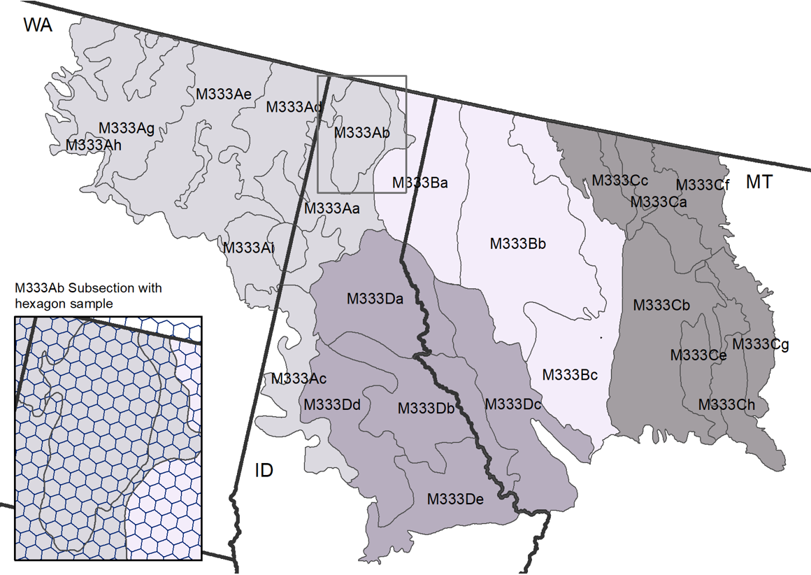
Figure 1: Simulation study area.

The FIA program surveys a sample of field plot locations across the US based on a hexagonal grid. Each plot samples approximately 2.5 acres (1.0 ha) of land and represents approximately 6000 acres (2428 ha) of land within each hexagon [32, 25]. A set of condition and tree-level attributes are measured and observed at each survey plot location and stored in FIA’s national database [29]. We extracted data from FIA’s database (last updated 2021 July 8) on 20 July 2021. There are 3946 survey plots across the 23 domains, with 98% of the plots measured between 2010 and 2019. From these plots, we compile our Y-variables and associated X-variables.

Our Y-variables were all aggregated to the plot level. These variables were: basal area (BA), net cubic-foot volume (VOLCFNET), net board-foot volume (VOLBFNET), number of trees (COUNT), aboveground dry biomass (DRYBIO), and aboveground carbon (CARBON). See Table 1 for further details.

Variable	Units	Description
BA	square feet	Basal area of live trees
VOLCFNET	cubic feet	Net cubic-foot volume in sawlog portion of a live sawtimber tree
VOLBFNET	board feet	Net board-foot volume in sawlog portion of a live sawtimber tree
COUNT	number	Number of live trees per acre unadjusted
DRYBIO	tons	Aboveground biomass of live trees [33]
CARBON	tons	Aboveground carbon of live trees [33]

Table 1: Y-variables or survey variables recorded by field crews at each surveyed plot.

We also have auxiliary X-variables from satellites, climate records, and digital elevation models that were thought to relate to and discriminate our Y variables (Table 2). The auxiliary information includes surface reflectance images, including spectral indices and classified imagery to get a picture of vegetation on the ground [34] and both broad-scale and localized climatic characteristics to understand ecological tolerances. All auxiliary data were resampled from their original resolution to 90x90m pixels. For each plot, we have the auxiliary data corresponding to that plot’s location. While Table 2 lists all auxiliary variables available to us, our kNN matching steps only used the categorical variable wc2cl for stratification and the quantitative variables tcc, elev, eastness, northness, tri, tpi, ppt, tmin01 for matching. Some of our analyses in Section 5 used tnt for post-stratification.

Variable	Units	Description
ndvi	index	LANDFIRE 2010 Landsat Normalized Difference Vegetation Index [35, 36, 37]
evi	index	LANDFIRE 2010 Landsat Enhanced Vegetation Index [35, 36, 37]
tcc	%	National Land Cover Dataset (NLCD) Analytical Tree Canopy Cover [38]
elev	meters	LANDFIRE 2010 DEM - elevation [39]
eastness	(-100 to 100)	Transformed aspect degrees to eastness [39]
northness	(-100 to 100)	Transformed aspect degrees to northness [39]
rough	meters	Degree of irregularity of the surface [39]
tri	index	Terrain Ruggedness Index [39]
tpi	index	Topographic Position Index [39]
ppt	mm$\times$100	PRISM mean annual precipitation - 30yr normals (1991-2020) [40]
tmean	∘C$\times$100	PRISM mean annual temperature - 30yr normals (1991-2020) [40]
tmax	∘C$\times$100	PRISM mean annual maximum temperature - 30yr normals (1991-2020) [40]
tmin	∘C$\times$100	PRISM mean annual minimum temperature - 30yr normals [40]
tmin01	∘C$\times$100	PRISM mean minimum temperature (Jan) - 30yr normals [40]
tdmean	∘C$\times$100	PRISM mean annual dewpoint temperature - 30yr normals (1991-2020) [40]
vpdmax	Pa$\times$100	PRISM max annual vapor pressure deficit - 30yr normals (1991-2020) [40]
def	mm	TOPOFIRE mean annual climatic water deficit - 30yr normals (1981-2010) [41]
wc2cl	class	European Space Agency (ESA) 2020 WorldCover global land cover product [42]
tnt	class	LANDFIRE 2014 tree/non-tree lifeform mask [43, 44]

Table 2: X-variables or auxiliary variables.

As a basis for the artificial population, besides the survey sample we also have complete auxiliary-only data for the full population: around 12 million pixels from around 4000 different hexagons, with around 3000 pixels per hexagon. For each of these auxiliary-only pixels, we had the same $X$ variables as for the 3946 pixels corresponding to the real survey plots, with a few exceptions: (1) We also had tmax in the real survey+auxiliary “donor” dataset, but not in the auxiliary-only “recipient” dataset. (2) We also had TMb5 and tnfdef in the “recipient” data but not in the “donor” data.

We use an analysis function in the FIESTAnalysis R package (which is an extension of the FIESTA R package), anGetPixeldat(), to generate pixel-level data tables for each subsection [45, 46]. The function creates a table of a combination of longitude and latitude extracted from each 90x90m pixel across each subsection, including a unique identifier of each pixel. This table is then used to extract values of our auxiliary information to create a set of data for our simulation models.

2 Population Generation and Design-Based Sampling

2.1 Population Generation with KBAABB

Because we have rich auxiliary data for the entire population, as well as a survey sample dataset that contains both the auxiliary and response variables for each sampled observation, we can treat the unobserved response values in our population as missing data that needs to be imputed.

Two popular approaches to imputation of missing data are based on nearest neighbors (NN). In the single NN approach, each recipient row is matched to the “nearest” donor row—the donor row whose auxiliary variables are most similar to the recipient’s—and that donor’s response variables are imputed to that recipient. However, this approach is unsuitable for multiple imputation, because the same donor will always be imputed to the same recipient. An alternative is to find a recipient’s $k$ nearest neighbors (kNN) to be the donor pool, for a $k$ such as 5, 10, or 20 [18], and then to randomly choose one case in this donor pool to be imputed to the recipient [47]. This avoids single NN’s problem of always imputing the same donor—but it can also lead to bias in the imputed conditional distributions of $Y|X$, since a larger donor pool may include $Y$ values that are not actually realistic for the recipient’s $X$ values. A third possible approach that we do not explore here would be to impute a mean or median of the kNN donor pool [22]. This may be reasonable for imputation when the goal is only to estimate means or medians, but it would make the imputed variances too low to realistically represent the whole distribution of Y values [48].

Instead, KBAABB is based on the approximate Bayesian bootstrap (ABB), in which we would first draw a bootstrap sample with replacement from the complete-data cases, then draw with replacement from this bootstrap sample to impute the missing cases [12]. Typically we impute from a smaller donor pool based on some auxiliary information, rather than imputing uniformly from the entire bootstrap sample, in order to reduce both bias and variance. If we use a single NN from the bootstrap sample to define the donor pool for each recipient, this combination of NN with ABB avoids the issue of always imputing the same donor that arises under single NN imputation alone. Yet it also avoids adding too much of the bias that can result from using kNN with a large donor pool: the probability of a given donor being in the bootstrapped donor sample is asymptotically 63.2% ($1-e^{-1}\approx 0.632$), so the original sample’s single NN for a given recipient will still be imputed around 2/3rds of the time [15].

However, NN with ABB is still computationally expensive. In multiple imputation of missing data, we need to take a new bootstrap sample and redo the NN search for each recipient every time we want another imputed dataset. Meanwhile for our own task of generating an artificial population, it would not make sense to bootstrap only once and impute the entire population from that one bootstrapped sample: the variability in Y would be too low given the bootstrapped sample, and the variability “across bootstrap samples” would be too high because we only took one. Taking a new bootstrap sample for every recipient row would be conceptually more reasonable, but too computationally expensive in practice. KBAABB is a shortcut designed to approximate this latter approach.

KBAABB first uses the original sample (not a bootstrap resample) to find a donor pool of $k$ NNs for each recipient row separately. Then, to mimic the fact that an ABB donor is in roughly 63.2% of bootstrap samples, KBAABB uses weighted sampling to choose one of the donors for each recipient. For each recipient, there is a 63.2% chance that its full-donor-sample’s first NN would be in the bootstrap sample, so we select it with probability 0.632. There is also a $(1-0.632)\times 0.632$ probability that the first NN would not be in the bootstrap sample but the second-nearest neighbor would be, so we select the 2nd-NN with probability $(1-0.632)\times 0.632\approx 0.233$. Similarly, we select the $j^{th}$ NN with probability $(1-0.632)^{j-1}\times 0.632$. In practice, this probability becomes negligible beyond $j=8$ or $j=9$, so we only find the $k=10$ NNs and select the $10^{th}$ NN with probability $1-\sum_{j=1}^{9}(1-0.632)^{j-1}\times 0.632\approx 0.000124$.

Conceptually and empirically, KBAABB allows for more realistic variability in Y than single NN, and less bias than kNN imputation with large k. Computationally, KBAABB costs no more than kNN with $k=10$, which is far less expensive than actually rerunning a full iteration of ABB for every recipient row in the artificial population. Theoretically, KBAABB should be a good approximation to ABB, and thus inherits ABB’s properties of “valid” inference under both Bayesian and design-based frameworks.

Let us briefly review how “valid” inference is defined in the setting of multiple imputation for missing data, before we connect it to our artificial population setting. In the case of missing data due to nonresponse, [14] requires us to have (1) a statistic $\hat{Q}$ which is unbiased for population parameter $Q$ under the sampling design when we have complete data (no nonresponse or missingness); and (2) a complete-data variance estimator $\widehat{\mbox{Var}}(\hat{Q})$ which is similarly unbiased for $\mbox{Var}(\hat{Q})$, the true design-based variance of $\hat{Q}$. Then, by saying that our repeated-imputation inference is “valid” in the design-based sense, we mean that $\bar{Q}_{m}$ (the average of $\hat{Q}$ across $m$ imputations) is asymptotically unbiased for $Q$ under both the sampling and nonresponse mechanisms; and that we can find a repeated-imputation variance estimator $T_{m}$ which is asymptotically unbiased for $T_{0}$, the total variance of $\hat{Q}-\bar{Q}_{m}$ with respect to both sampling and nonresponse. For details, see Chapter 4 of [14], which shows that although simple hot deck imputation or single NN imputation is not “valid” in this sense, ABB is valid. In this sense, KBAABB should allow for valid repeated-imputation inferences too, if we were to use it for multiple imputation.

However, our present interest is in generating artificial populations, not in nonresponse. For us, $\hat{Q}$ might be one of the model-assessment metrics we describe in Section 4, such as the relative bias or confidence interval coverage of a particular SAE model; and $Q$ would be the expectation of that same metric across many draws from the real population. Then $\bar{Q}_{m}$ would be the average of $\hat{Q}$ across $m$ repetitions of generating an artificial population with KBAABB and drawing a design-based sample from it. By analogy with ABB, such a $\bar{Q}_{m}$ should be asymptotically unbiased for $Q$ across hypothetical repeated samples from the real population, and likewise we could develop an approximately unbiased variance estimator using $m$ repetitions of KBAABB.

Admittedly, we create only one “imputation”—a single artificial population—so asymptotic validity across multiple imputations is not the most directly relevant property for an artificial population to have. Still, it provides at least two forms of justification for using KBAABB: we can trust the KBAABB artificial population (1) as much as a Bayesian can trust a single draw from a posterior distribution, or (2) as much as a survey methodologist can trust a single imputation from an approximately design-unbiased repeated-imputation mechanism. Such justification is admittedly incomplete, but still stronger than completely ad hoc ways of forming an artificial population—much like taking a simple random sample is incomplete but still better than taking a convenience sample. This theoretical justification does not absolve us of empirical checks on the quality of our artificial population, but it can help tip the scales when deciding between KBAABB and other methods that appear empirically comparable but lack any formal backing.

We also briefly note that KBAABB’s interpretation as a posterior draw is different from “posterior predictive checks” as in [49]. Posterior predictive checks involve drawing new data from the posterior after fitting a posited model, as a way of checking the fit of that same model. By contrast, in ABB or KBAABB, the “model” whose posterior we draw from is essentially nonparametric (resampling from the observed data), used only to impute missing data or generate the artificial population. It is deliberately distinct from any models that we want to fit to the completed dataset(s) and use for complete-data inference.

To implement KBAABB, we must only decide how to define “nearest” for the kNN search: Which variables, transformations, and distance metric should be used to rank the donor pool for each recipient?

2.2 KBAABB Implementation in our FIA Setting

First of all, we decided to form strata or “donation classes” using the categorical variable wc2cl or World Cover 2-level classification: a “tree or nontree” classification for each pixel, based on satellite measurements. By imputing separately within wc2cl classes, we reduce the risk of unrealistically imputing a heavily-forested pixel’s Y values to an unforested pixel and vice versa. Additionally, wc2cl was the only categorical auxiliary variable, so using it to form donation classes allows us to use straightforward distance metrics (such as Euclidean distance) within each class since the remaining variables are all quantitative.

Next, kNN is known to suffer from the curse of dimensionality: if we use something like Euclidean distance in a high-dimensional space, the several nearest neighbors might all be very far away [50]. When there are many auxiliary variables available for matching, NN imputation can be asymptotically biased and some analysts prefer to summarize the auxiliary variables into a univariate matching variable [51], for instance using predictive mean matching: build a predictive model on the complete data, apply it to each recipient row to get a predicted value, and impute from the $k$ donors whose responses are closest to this prediction [18]. However, in our case we wished to keep the matching process as model-free as possible, so we preferred to simply reduce our matching space to a subset of the variables. Another rationale for using a subset of the variables is that such parsimony can reduce unnecessary variance in the matching process [23]. On the other hand, [52] argues that imputation should use as many auxiliary variables as possible because the missing at random (MAR) assumption becomes more believable as we condition on more information, and the same argument appears reasonable in our own setting of creating an artificial population.

As we had access to subject-matter experts with detailed knowledge of the auxiliary variables, we relied on their expertise to choose a subset of 8 out of the 16 available variables for matching. These 8 variables were chosen so that they all measured distinct concepts and were thought to be at least somewhat predictive of the Y variables to be imputed. As a quality check, we confirmed that the selected subset of X variables had low pairwise correlations within each wc2cl donation class, in the full population as well as in the survey sample. At this point, the curse of dimensionality and high variability were deemed not to be major concerns.

Next, we transformed the most heavily skewed of the selected variables to be more symmetric. Otherwise, donors with distant outlier values might never be one of the nearest neighbors for any recipient. [53] show that for imputation purposes, NN imputation can be biased when the matching variables are not symmetric. Right-skewed variables were transformed as $\log(c_{j}+X_{j})$ and left-skewed variables as $\log(c_{j}-X_{j})$, with a separate constant $c_{j}$ chosen for each variable $X_{j}$ to ensure positive values inside the logarithm. While these simple log-transformations achieved adequately symmetric data for our purposes, alternative approaches to transforming survey data for imputation are suggested in [54].

After this step, we also centered and scaled each of the selected variables to have mean 0 and standard deviation 1 (within each wc2cl class separately) on the full-population auxiliary dataset. The same centering and scaling constants (by class and variable) were then applied to the smaller survey sample dataset. This removed the effect of different variables having different units and scales, ensuring that each variable would have effectively the same weight in the kNN matching process [50].

With these selected and transformed variables, we confirmed again that the pairwise correlations were still very small. This allowed us to use simple Euclidean distance instead of something like Mahalanobis distance that would account for covariances between variables [22].

The software we used to carry out the kNN matching step was the FNN R package [55]. For every recipient row, we match on the selected, transformed variables to find its donor pool of 10 NNs. We use the bootstrap-probability-based weights described above $(0.368^{j-1}\times 0.632)$ to sample one of each recipient’s 10 possible donors. Finally, we impute all 6 of the response Y variables from that donor to the recipient. If instead we were to impute each response variable independently, our artificial population would not accurately reflect the associations among these variables [19]. Similarly, [56] imputed missing responses for food and alcohol consumption in pairs (current consumption and consumption 5 years ago), because imputing them separately could misrepresent the nature of within-respondent changes in consumption over time.

To define the population means for each Y variable and domain that are our targets of estimation in the simulation study, we simply take the mean of that Y variable across all of that domain’s pixels in the artificial population.

In Appendix A, we show a sensitivity analysis on the probabilities of selection and the choice of $k$, comparing KBAABB to an unweighted kNN approach where donors are sampled uniformly at random from pools of the recipient’s $k$ nearest neighbors. For each response variable Y, we found the same results: As kNN’s $k$ grows, the standard deviation of Y in each domain becomes more similar across domains. For the smallest $k$ = 1, 5, or 10, as well as for KBAABB, the standard deviations of Y by domain in the artificial population are similar but not identical to those in the original sample, but $k$ = 20 or larger makes the domains too similar to each other. Furthermore, when looking at maps of the imputed Y values, the spatial patterns look realistically smooth for $k$ = 1 and for KBAABB, but begin to look unrealistically noisy for $k$ = 5 or larger. Setting aside the loose theoretical justification behind KBAABB, we chose to use KBAABB to avoid the worst-case risks of kNN with $k$ = 1, although kNN with $k$ = 1 or $k$ = 5 could have been defensible choices as well.

Section 3 describes the other diagnostics and sensitivity checks we carried out on the resulting artificial population.

2.3 Alternatives

A simpler approach to design-based simulations could have been to bootstrap or subsample directly from our survey dataset. However, in the FIA setting, we were fortunate to have auxiliary data for the complete population: every one of the roughly 12 million 90x90m pixels in EcoProvince M333. By resampling only from the survey dataset, we would miss the opportunity to use the rich information we have about how the sampled pixels differ from the rest of the population.

When creating an artificial population that does use this complete dataset, one approach could have been to simply treat one of the X variables as our response variable, for example as in [6]. However:

• Most of our X variables do not look much like our Y variables of interest. For example, COUNT is zero-inflated, but most of the auxiliary data are not. Using one of these Xs as the Y would not help us with model diagnostics and model selection for the actual Ys of interest.

• Some of the more realistically response-like X variables are transformations of each other, which could make the modeling problem too easy to be useful. For example, ndvi is defined using much of the same raw data as evi, and they are highly correlated. If we used one of them as Y and the other as an X variable, then simple models would fit well, but this would not help us know whether our models would fit well to the real Y variables.

• We want to know how well each of these Xs can be used to predict our actual Ys. If we use one of these Xs as a response instead, we cannot know how good of a predictor it is.

Another approach could be to make up a parametric model (or fit one to the sample); make a prediction $\hat{Y}(X_{i})$ for each row of the Xs; and add random noise to each prediction to generate the Ys for our artificial population. However, under this approach, the artificial population would inherently favor certain models. If the “true” artificial Ys are generated from a linear model, for example, then a linear model for the SAEs is almost certain to look best in our model comparisons; yet that might not be true of the Ys in the real population we care about. For our purposes, simulated or imputed Y values need to be generated using a different model than any of the SAE models we are planning to evaluate. Put another way, if the models we want to evaluate are quite likely mis-specified in the real population, then they should be mis-specified in the artificial population as well. Additionally, adding noise to model predictions would not match certain features of the real Ys (such as being zero-inflated) without considerable fine-tuning. This is a concern whether the noise comes from a parametric model or from donating residuals from the model fit to the original sample, as in the “local residual draws” approach [18].

Instead, we generated realistic unit-level data by KBAABB, a “kNN-based approximation to ABB.” It differs from the “parametric model plus noise” idea above in two important ways:

• Instead of using a parametric model to make predictions and add noise to them, we use $k$-nearest-neighbor matching. This ensures that our imputed Y values will have reasonable conditional distributions $Y|X$. However, they are chosen nonparametrically, so that when we evaluate possible parametric models to use as SAEs, the artificial population will not have a bias towards being fit well by these same parametric models. (Of course, if we also planned to evaluate the use of kNN-based models for SAEs, then we would want to choose a different non-kNN model to generate our artificial population, as noted in [57].)

• We choose one of these $k$ “nearest” Y values at random (using the bootstrap-based weights as described above). If instead we always used the single nearest neighbor, or always used the mean of all $k$ nearest neighbors, it could result in unrealistically low levels of variation in the imputed Y values; see [15] and our Appendix A.

The downside to kNN or ABB based approaches, including KBAABB, is that we can never impute plausible Y values that exist in the real population but were not observed in the sample survey data. We did not deem this to be a major concern in our FIA example, because we had observed several thousand distinct response values for each Y variable in our survey dataset and they covered most of the range of plausible population values for each Y variable.

2.4 Sampling for Design-Based Simulations

The artificial population consists of around 12 million pixels, each with hexagon IDs, for a total of around 3000 pixels per hexagon out of the approximately 4000 hexes.

For each replication (“rep”) of a survey sample from this population, we take a sample of one pixel per hexagon, with pixels chosen uniformly at random with each hexagon. This is approximately a form of systematic sampling, since the hexagons uniformly tile the geographic area of interest. Then we drop any locations that happen to fall outside province M333. We sampled 2500 such reps, in order to carry out design-based simulations which respect the sampling design of the actual survey data. When we fit a model across reps, and summarize the model’s empirical properties across reps, these properties are reasonable stand-ins for what we could expect to see under repeated sampling from the real sampling design.

In future refinements, we could add a simulated non-response stage after the sampling stage, to mimic the limited non-response behavior seen in the real survey.

3 Empirical Diagnostics

To check whether the artificial population generated with KBAABB looked reasonable, we compared the statistical distributions of the imputed Y variables to the original survey, and we compared the spatial smoothness of the imputed Y variables to that of similar X variables. We also looked for imbalances in how often each donor was used, and in how often each recipient’s domain matched the donor’s domain. We repeated these checks for each of the 6 Y-variables and found similar results, so for brevity most examples in this section are illustrated using a single Y variable: BA (basal area).

First, we confirmed that marginal distributions and pairwise scatterplots from the artificial population resembled the real survey data. For marginal distributions, we compared the original and imputed values of each variable using histograms or eCDFs (empirical cumulative distribution functions), as in Figure 2. Histograms are more familiar to many readers, but eCDFs do not require us to choose a bin size and can also make it easier to compare behavior in the tails. With either graph type, we found that each Y variable’s marginal distribution did not change substantially between the survey and the artificial population. Similarly, we found that pairwise scatterplots (pairs plots) of the Y variables did not differ much between the survey and the artificial population (Figures 3 and 4).

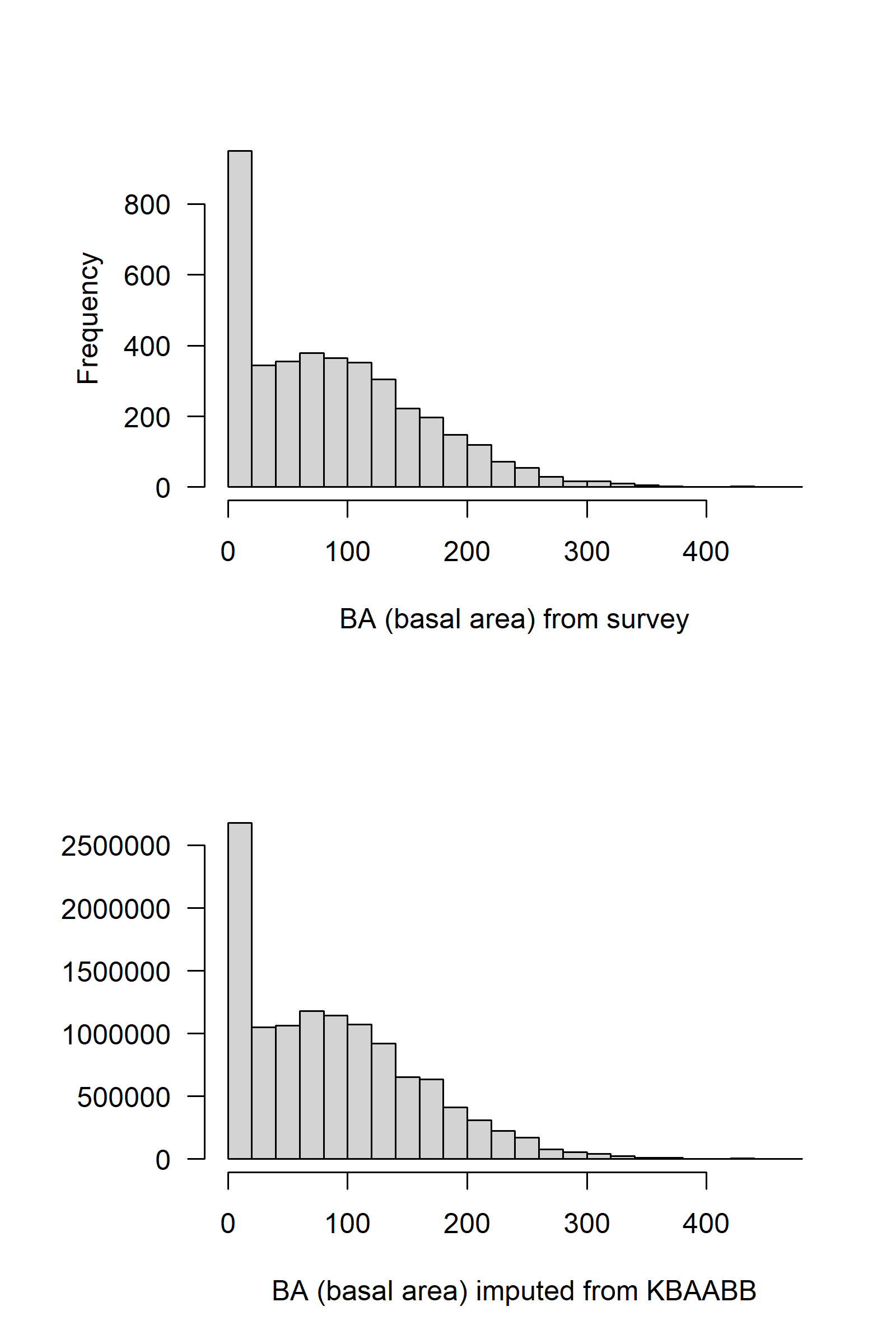
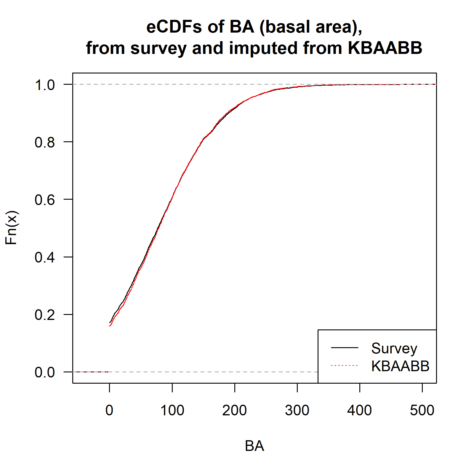
Figure 2: Histograms (left) and empirical CDFs (right) of original vs imputed BA (basal area).

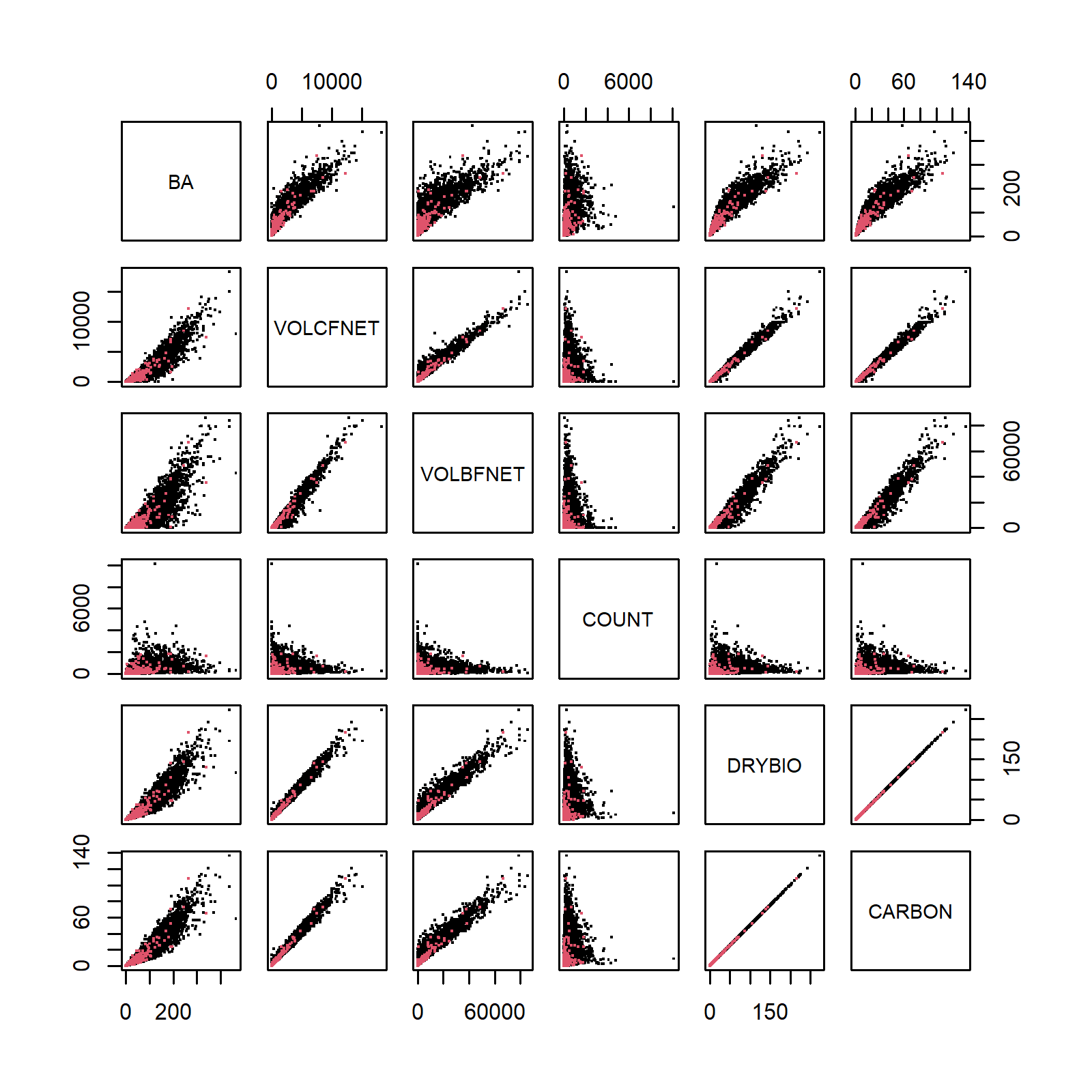
Figure 3: Pairwise scatterplots of original Y variables. Color shows wc2cl: black = class 1, red = class 2.

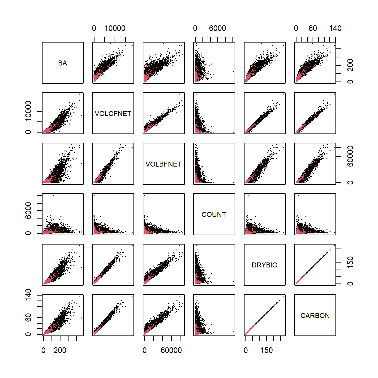
Figure 4: Pairwise scatterplots of Y variables imputed using KBAABB (on a 1% subsample of the artificial population, due to slow plotting of 30 graphs of full dataset’s 12 million points). Color shows wc2cl: black = class 1, red = class 2.

Next, we checked how well the imputed domain-level standard deviations (SDs) match the real survey SDs in each domain. Figure 5 shows that for each Y-variable, the KBAABB artificial population’s domain-level SDs are strongly but not perfectly correlated with their original-sample counterparts. This is a good sign, because if they were perfectly correlated we might simply be reproducing the original sample, while if they had low correlations we might be imputing unrealistic donors to each recipient. By contrast, we show a similar example using kNN with varying values of $k$ in Appendix A.

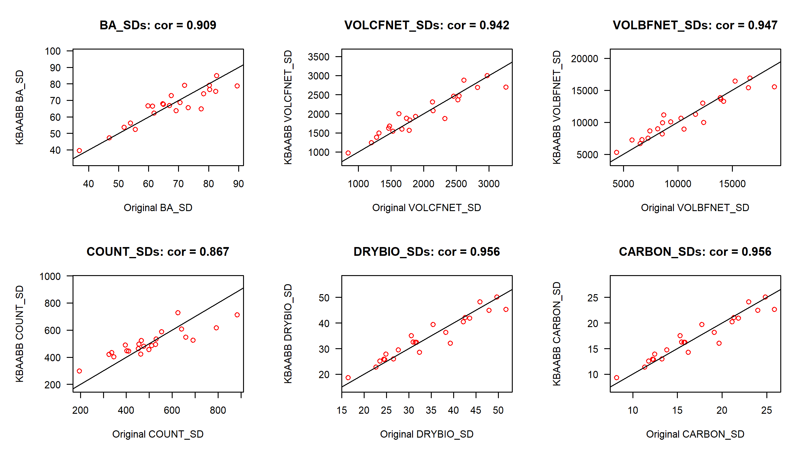
Figure 5: Original vs imputed SDs of each Y-variable for each subsection, using KBAABB. All plots show $y=x$ line as a common reference.

We also checked whether the spatial smoothness of imputed Ys looks reasonable compared to the spatial smoothness of Xs, for which we have the complete population data. For example, looking at a small portion of the map (zoomed in so that we can see each pixel in adequate separately), the spatial patterns in the imputed variable BA (Figure 6) appear to be only a little noisier than spatial patterns for related auxiliary variables tcc and ndvi (Figures 7 and 8). We report further checks in Appendix A, where we see similar maps for the other Y variables when using KBAABB, as well as when using kNN with k=1 or 5; but all maps look much too noisy when using kNN with k=10 or greater.

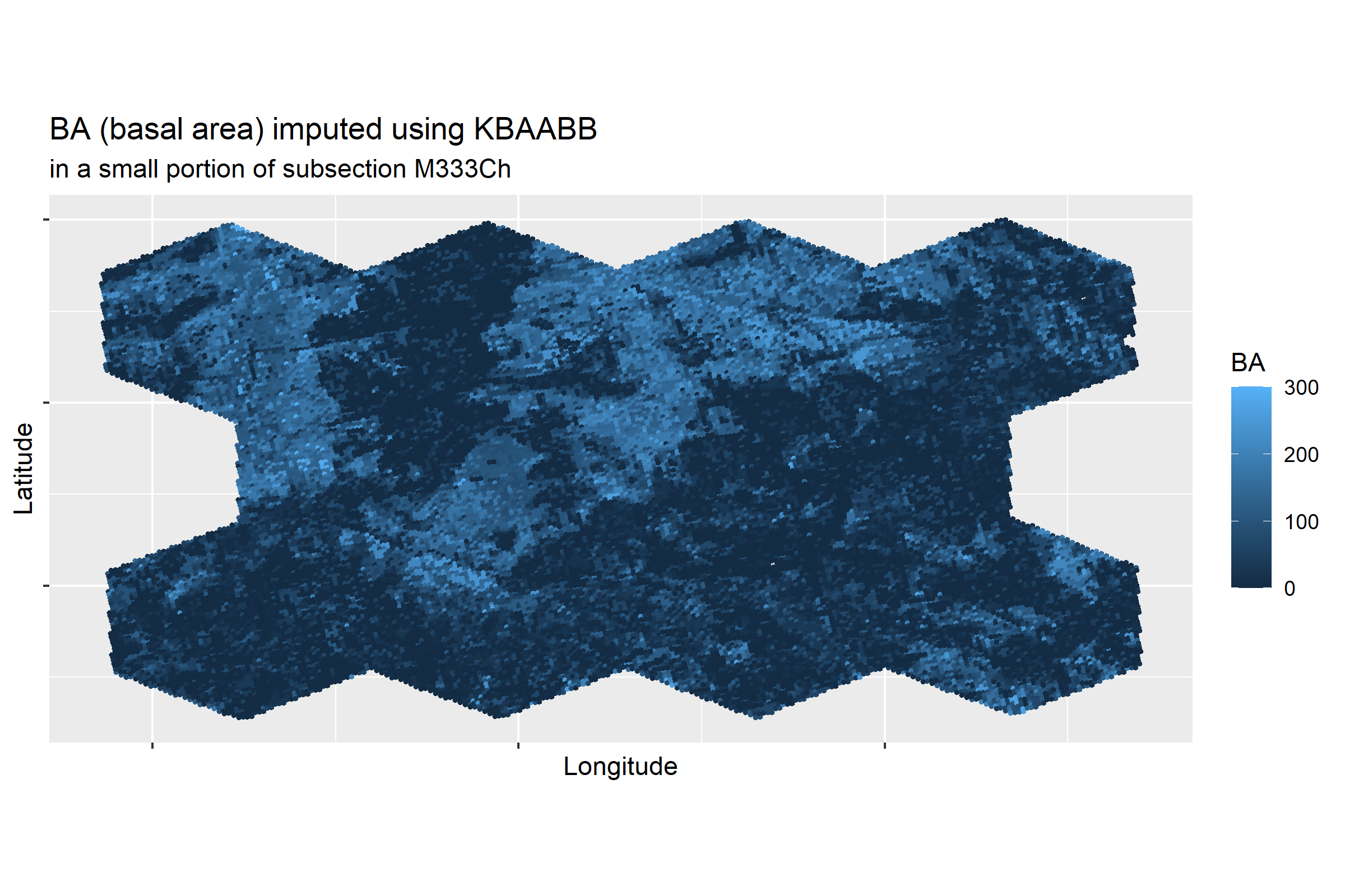
Figure 6: KBAABB imputation of BA (basal area) in a portion of subsection M333Ch.

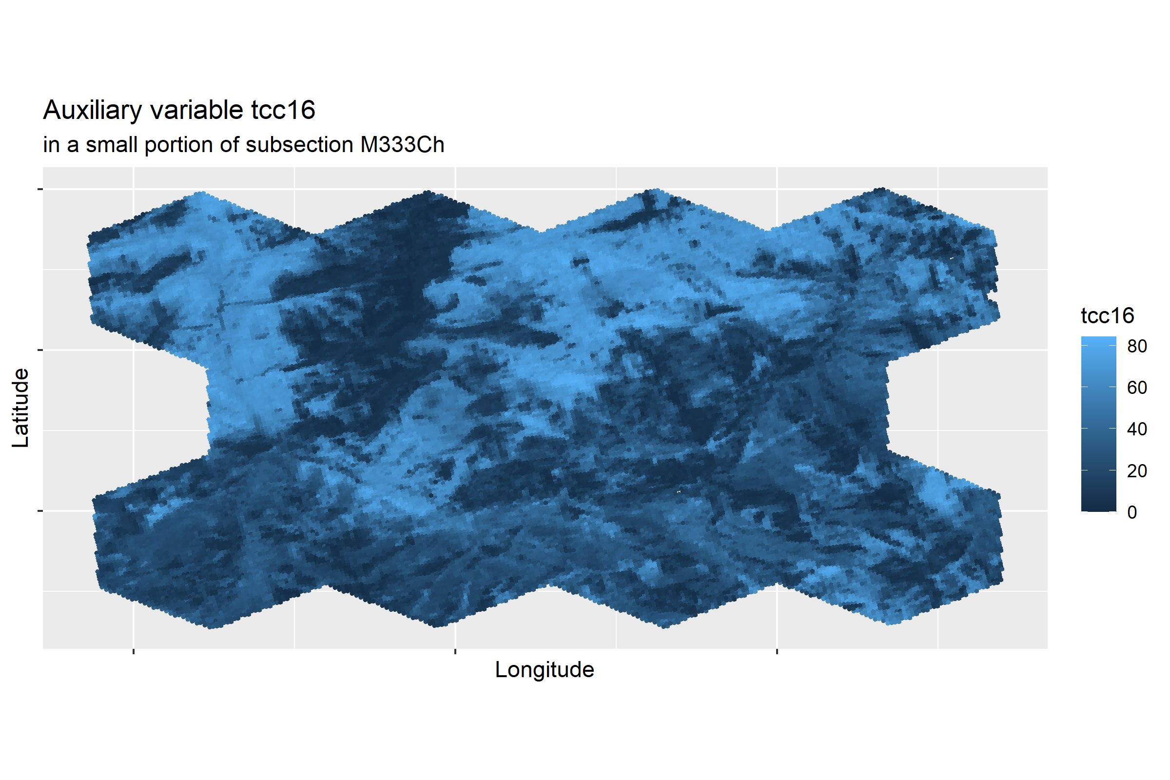
Figure 7: True values of auxiliary variable tcc (tree canopy cover) in a portion of subsection M333Ch.

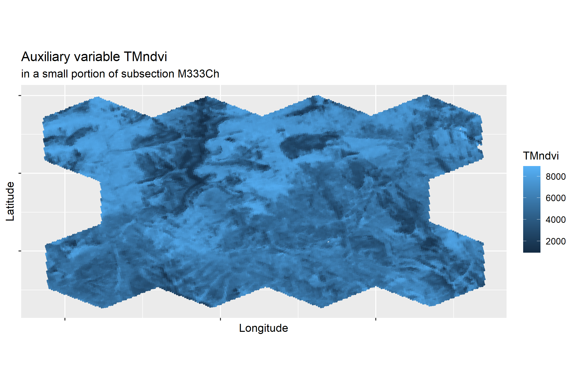
Figure 8: True values of auxiliary variable ndvi (Normalized Difference Vegetation Index) in a portion of subsection M333Ch.

Next, we checked how often each of the 3946 donor rows were used (Figure 9). Recall that for each recipient row, KBAABB finds its 10 NNs among the donor rows and then uses weighted sampling to choose one donor. Hence, first we checked how often each donor was included in a donor pool of some recipient’s 10 NNs (left side of Figure). For both wc2cl classes, most donors were chosen to be in 10,000 to 50,000 donor pools, though some were chosen for as many as 69,302 donor pools while others for as few as 1 or 0 donor pools. Every one of the 3101 donors in class 1 was in a donor pool at least once, and 811 of the 845 donors in class 2 were in a donor pool at least once. Next, we repeated the analysis but to see how often each donor row was actually used as a donor (right side of Figure). For both classes, most donors were actually used for 1,000 to 5,000 recipients, though some were used as many as 9,173 times while others were only used 1 or 0 times. Again every one of the 3101 donors in class 1 was used as a donor at least once, but 790 of the 845 donors in class 2 were used as a donor at least once. In short, only 55 of the possible donors were never used (all in wc2cl class 2); 34 of them were never in a donor pool, and the other 11 were simply never chosen by the weighted sampling. We are not concerned about these few never-used donors, because they all came from the non-tree class, in which most of the Y-variables are all 0s. The other possible donors were typically used a moderate number of times, with few over-used or under-used donors.

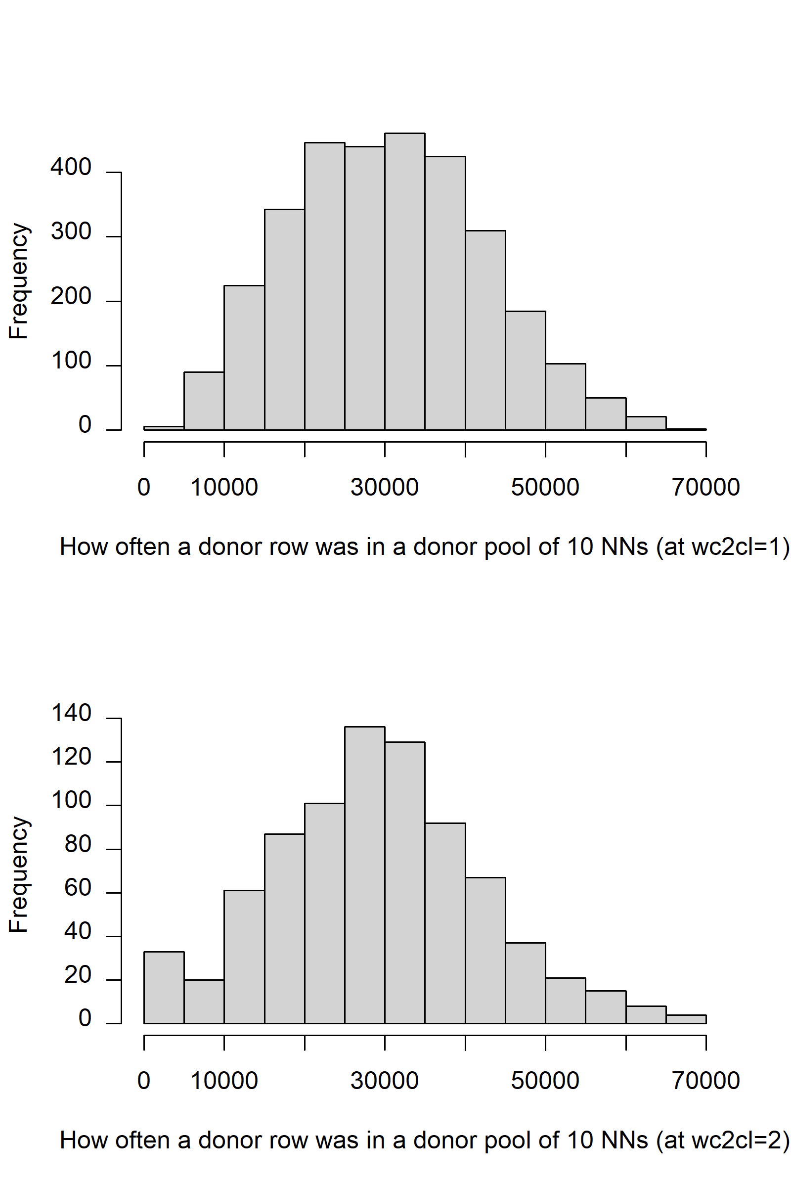
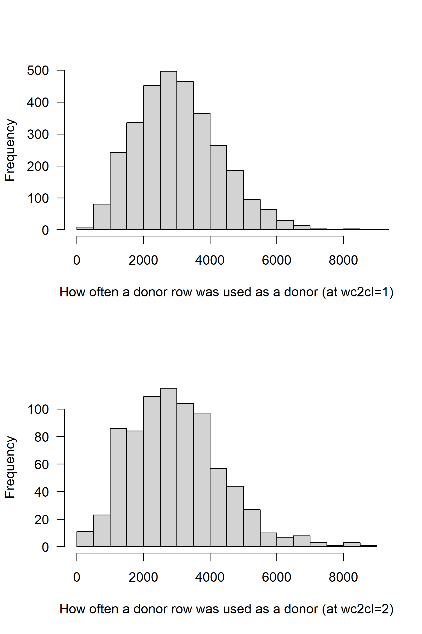
Figure 9: Count of how often each donor row was included in a donor pool of some recipient’s 10 nearest neighbors (left) or actually used as a donor (right), for wc2cl classes 1 (top) and 2 (bottom).

Finally, we cross-tabulated the domain of each donor vs. each recipient to see whether recipients tended to get donors from the same subsection; from a different subsection but still the same section; or from elsewhere (Figure 10). Within each column (recipient), the highest frequencies tend to be in the corresponding row (donor) or another row in the same section (regions separated by black lines), showing that recipients often but not always tended to get donors from the same subsection or at least the same section. If all counts had been only on the main diagonal (each domain’s imputed values all came from the same domain), we would have been concerned that the artificial population is too similar to simply taking copies of the survey sample. On the other hand, if counts were completely uniform, we would have been concerned that recipients are getting donors which do not actually resemble them. As it is, we feel comfortable seeing that our results fall between these two extremes.

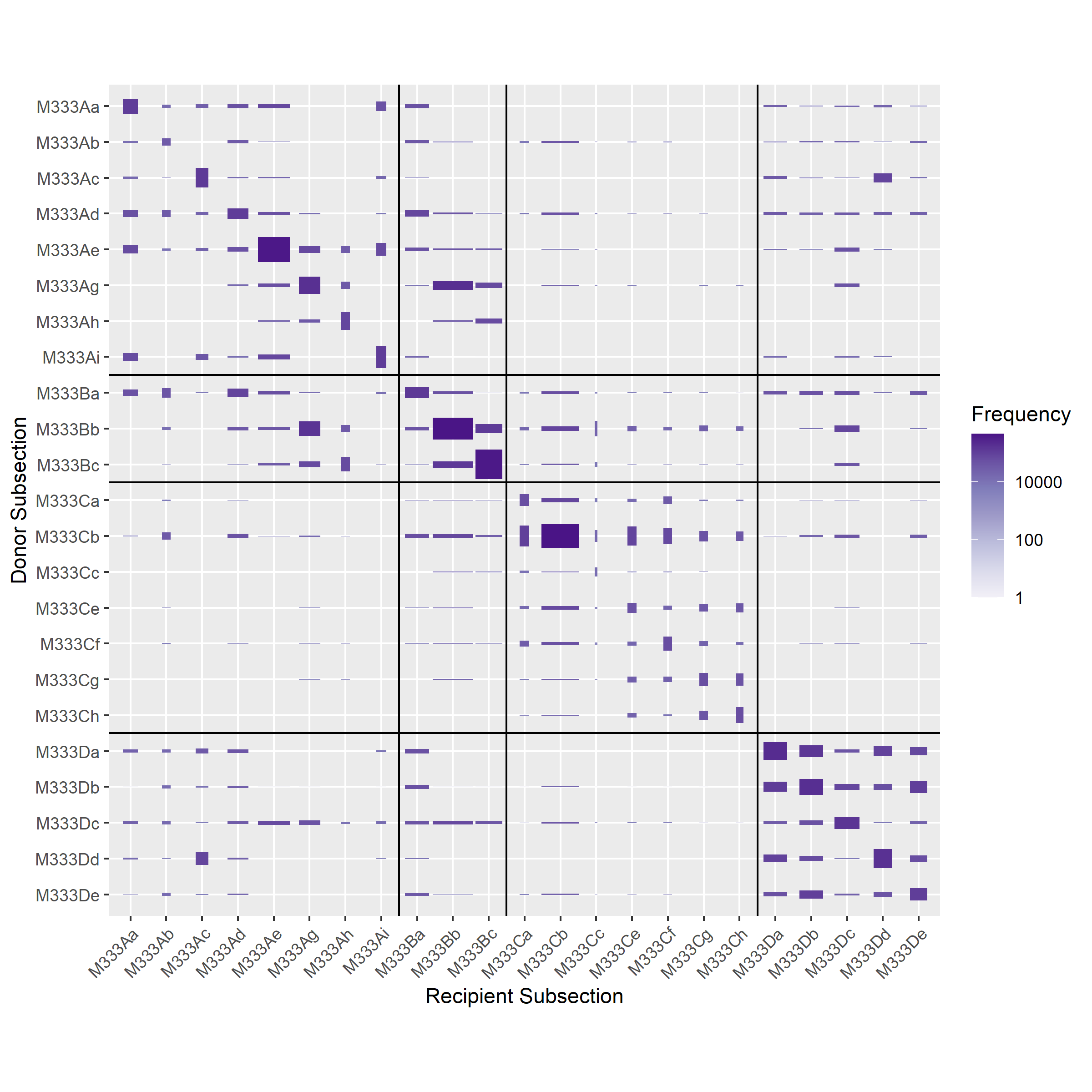
Figure 10: Count of how often donors from each subsection were used by recipients in each subsection. Box widths (fixed within each column) are proportional to the total number of pixels in each recipient subsection. Box heights (varying within each column) are proportional to the number of times a donor from that subsection was used for a recipient in that subsection, scaled so that boxes along the main diagonal would be squares if each conditional proportion (how often did that recipient use donors from its own subsection?) was equal to the overall proportion (31% of recipient pixels got donors from their own subsection).

4 Case Study

The artificial population generated with KBAABB allows for an extensive evaluation of SAE methods and strategies that may be implemented by researchers and others interested in the performance of small area estimators under a variety of conditions. In order to evaluate such small area estimators, we created 2500 samples from the artificial population, where we sampled one pixel per hexagon for each hexagon that overlaps M333, as described in Section 2.4. Next, for this case study, we reduced the sample size of the sample to 75%, 50%, and 25% of the original sample size for each replicate sample and assessed four estimators on each of these four collections of 2,500 samples. These estimators are assessed based on their estimates and variance estimates of average biomass (DRYBIO) within each subsection in M333. Varying sample size is just one of many potential “dials” one can turn to evaluate estimators; one could choose, for example, to vary the borrowing scope of some estimators, or to vary the number of small areas being used for modeling, or a variety of other dials. We have chosen to vary sample size and to use four commonly applied estimators in small area estimation literature to give a sense of what can be done with KBAABB through a basic yet illustrative example.

As mentioned above, we have chosen to assess four estimators commonly applied in the small area estimation literature. In particular, we implemented Horvitz-Thompson [58], modified generalized regression (GREG) [59, 60], area-level empirical best linear unbiased prediction (EBLUP) Fay-Herriot [17], and unit-level EBLUP Battese-Harter-Fuller [16] estimators.

These estimators were implemented in R using the FIESTAutils function SAest.large() [61]. The Horvitz-Thompson estimator was fit without weights and hence its estimate and variance estimate are the sample mean and sample variance, respectively. The modified GREG estimator’s regression coefficients were fit with ordinary least squares and the estimate and variance estimate were created based on the standard equations described in [4]. The Fay-Herriot and Battese-Harter-Fuller estimators were fit with restricted maximum likelihood to ensure unbiased estimation of the random effects.

We considered three evaluation metrics in this case study: relative bias, 95% confidence interval coverage, and mean square error ratio. The relative bias is defined as, for a particular estimator ($i$) and area of interest ($j$),

$$\frac{E[\hat{\mu}_{ij}]-\mu_{ij}}{\mu_{ij}}$$

where $\mu_{ij}$ is the true mean biomass for estimator $i$ in subsection $j$ as generated by KBAABB and $E[\hat{\mu}_{ij}]$ is the empirical expected value for estimator $i$ of mean biomass in subsection $j$ across all reps. The 95% confidence interval coverage is defined as, for a particular estimator and area of interest, the proportion of samples across all reps where a given estimator’s 95% confidence interval contains $\mu_{ij}$. Finally, the mean square error ratio is defined as the ratio of the empirical expected value of the MSE estimator and the empirical MSE for a particular estimator,

$$\frac{E[\widehat{MSE}_{ij}]}{MSE_{ij}}$$

where $E[\widehat{MSE}_{ij}]$ is the empirical expected value of the MSE estimator for estimator $i$ in subsection $j$ across all reps, and $MSE_{ij}$ is the empirical MSE for estimator $i$ in subsection $j$ calculated using all reps. For this analysis, we consider these three metrics for each subsection and as averages over the subsections.

We first assess relative bias of the four estimators in Figure 11 across (subfigure A) and between (subfigure B) subsections. For the design-based estimators we see that across subsections the relative bias does not change significantly as we vary sample size with both estimators exhibiting little to no bias, as expected. In regards to the model-based estimators, the Battese-Harter-Fuller estimator stays between -1 and 1% relative bias for each sample across subsections. The Fay-Herriot estimator does exhibit some substantial negative relative bias across subsections in the lowest sample size simulation, with about -4% relative bias. When looking within subsections, a pattern begins to emerge for the Battese-Harter-Fuller estimator; we see positive relative bias for low average biomass subsections, and negative relative bias for high average biomass subsections. This may be due to too-extreme pooling due to the random effects, or due to model-misspecification at the unit level. We do not see this pattern as strongly for the Fay-Herriot estimator, as in most subsections we see negative relative bias. In general within subsections, for the model-based estimators, we see the magnitude of relative bias increases as sample size decreases.

We now move to assessing confidence interval coverage and mean square error ratio. Figure 12 displays the 95% confidence interval coverage for each of the four estimators assessed in this case study, and Figure 13 displays the ratio of estimated and empirical mean square errors. When examining the confidence interval coverage for each estimator across subsections, we see some initially suprising results: for the modified GREG, Fay-Herriot, and Battese-Harter-Fuller estimators we see an increase in confidence interval coverage as sample size decreases (with the exception of the 0.25 sample size for the Battese-Harter-Fuller estimator). Further, we observe some extreme cases of this within subsections M333Bc (modifed GREG), M333Aa (modified GREG and Battese-Harter-Fuller), and M33Ce and M33Ab (Fay-Herriot). These results make sense in light of Figures 11 and 13, where it is clear that for subsections M333Bc and M333Aa the MSE ratios take extreme values for the referenced estimators. This is even clearer in subsections M333Ah and M333Ai where the confidence interval coverage is essentially one for each sample size simulation and the MSE ratio is greater than three for each sample size simulation. The anomalies for the Fay-Herriot estimator in M33Ce and M333Ab displayed in Figure 12 can be explained by the large negative relative bias exhibited in Figure 11 and the extremely small MSE ratio for those subsections in Figure 13.

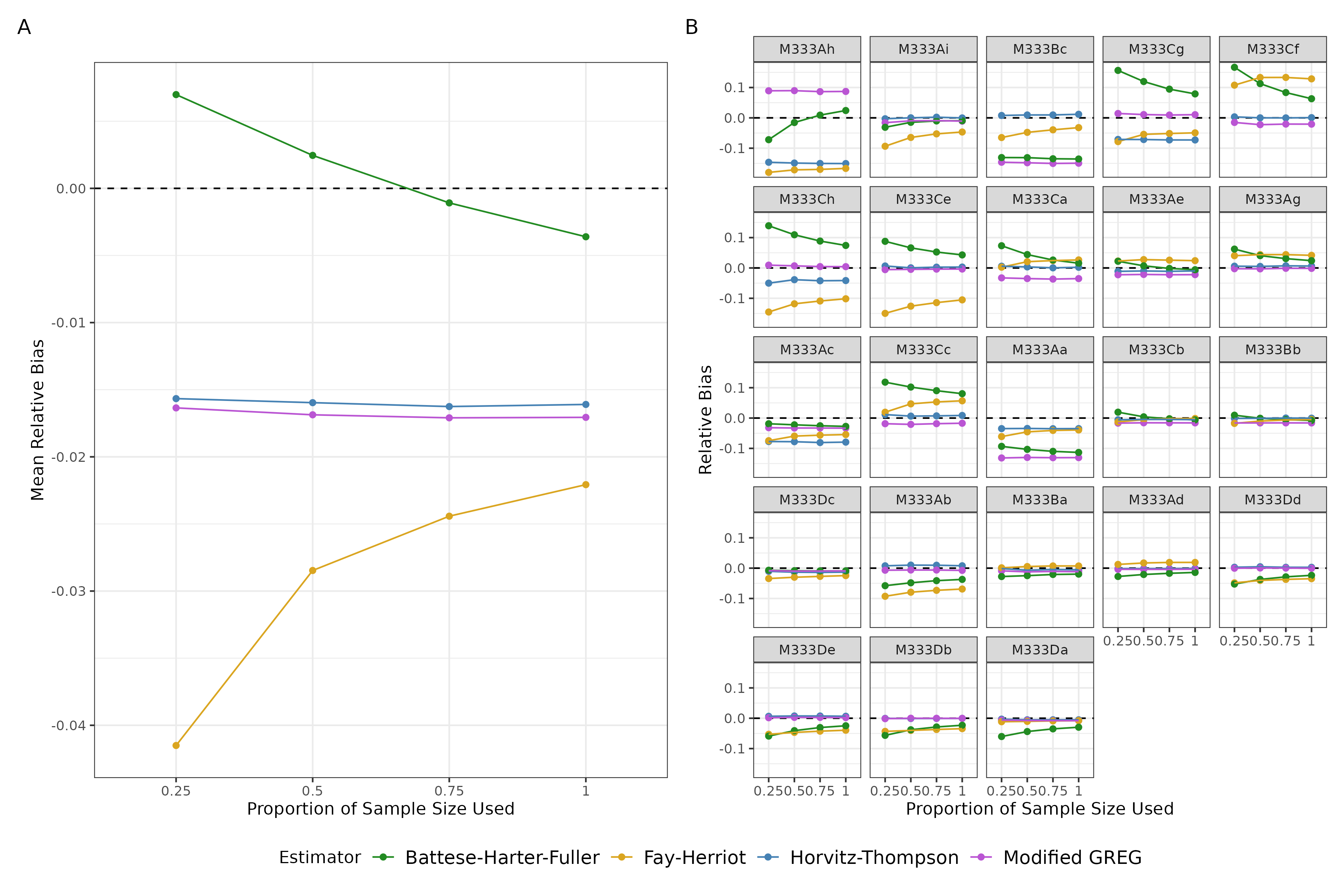
Figure 11: Relative bias of average biomass estimates across every and in each domain. Line and point color indicates the estimator used, and the x-axis corresponds to the proportion of the sample size used in each sample to produce estimates. Subfigure A shows the mean of the relative bias across domains and reps; Subfigure B shows relative bias averaged across reps, separately for each domain. The domains in Subfigure B are ordered by the true average biomass from the artificial population, least to greatest.

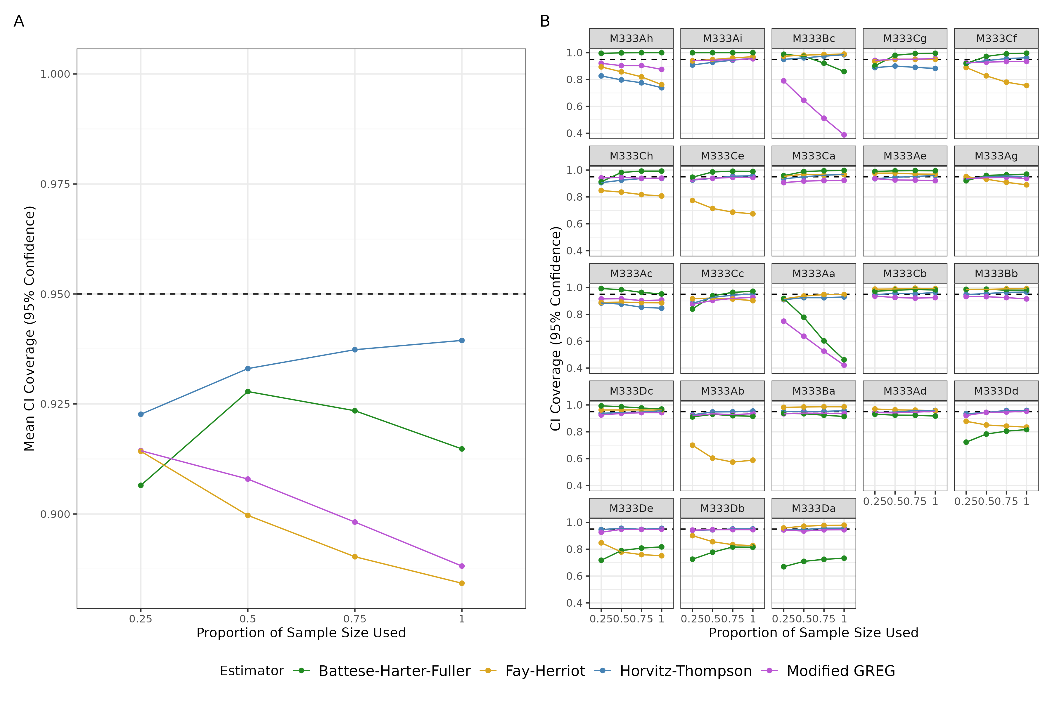
Figure 12: 95% CI coverage of average biomass estimates across every and in each domain. Line and point color indicates the estimator used, and the x-axis corresponds to the proportion of the sample size used in each sample to produce estimates. Subfigure A shows the mean coverage across domains and reps; Subfigure B shows coverage across reps, separately for each domain. The domains in Subfigure B are ordered by the true average biomass from the artificial population, least to greatest.

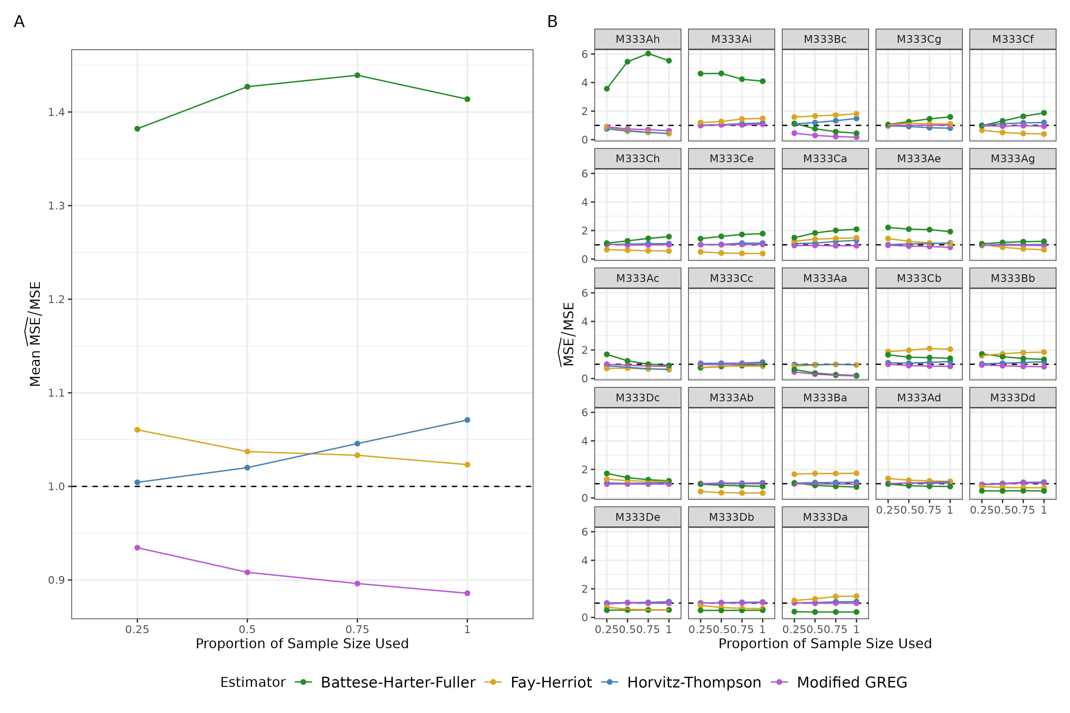
Figure 13: Ratio of estimated MSE and empirical MSE for average biomass estimates across every and in each domain. Line and point color indicates the estimator used, and the x-axis corresponds to the proportion of the sample size used in each sample to produce estimates. Subfigure A shows the mean of the MSE ratio across domains and reps; Subfigure B shows MSE ratios averaged across reps, separately for each domain. The domains in Subfigure B are ordered by the true average biomass from the artificial population, least to greatest.

5 R Shiny App

Alongside this paper we have created a draft R Shiny application [62] for exploring the artificial population and a few estimators. The app can be accessed at https://civilstat.shinyapps.io/fia-simpop-app/ and the code is available at https://github.com/ColbyStatSvyRsch/FIA-simpop-app. In our app we have not yet implemented the “dials” of Section 4, so at the moment it only displays estimates and metrics for samples mimicking the true sampling design.

For each of the 100 reps currently used in the R Shiny app, on each of the 23 domains we calculate three estimators: a direct (Horvitz-Thompson) estimator, a post-stratified estimator (using tnt for post-stratification), and a small area estimator using the unit-level Battese-Harter-Fuller model. The direct and BHF estimators and their variance estimates are as described in Section 4. The post-stratified estimator simply calculates direct estimates for each tnt class (tree or non-tree) in a domain, then weights them by the population proportions of each class in that domain. Each response variable uses a slightly different set of auxiliary variables in the linear regression for the BHF estimates (each model is specified on the app’s “About” page). Finally, for every domain and each of these three estimators, we calculate the relative bias; the $\widehat{\mbox{MSE}}/\mbox{MSE}$ ratio; and the 95% CI coverage, as in Section 4.

Even in development, the R Shiny app and artificial population have already been useful for helping us debug the R code for our SAEs. For example, the upper subfigure of Figure 14 shows a screenshot of how we noticed that our SAEs for Basal Area were consistently under-estimating the true values (but only for BA and no other response variables). This led us to notice a subtle bug in our SAE modeling code for the BA response variable. The fixed SAE model estimates are shown in the lower subfigure in Figure 14.

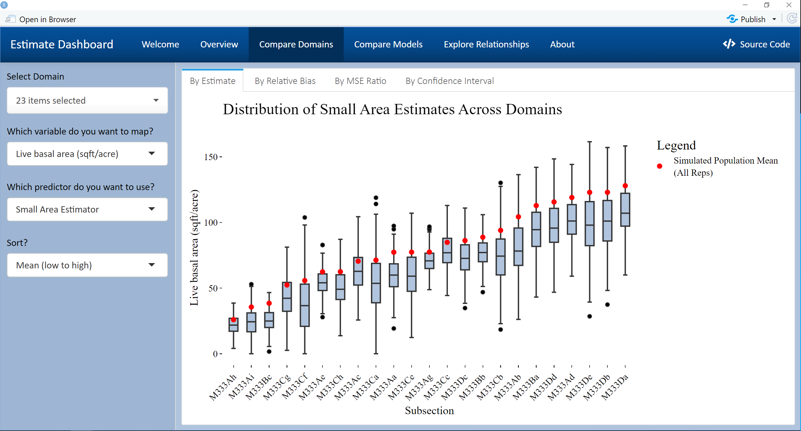
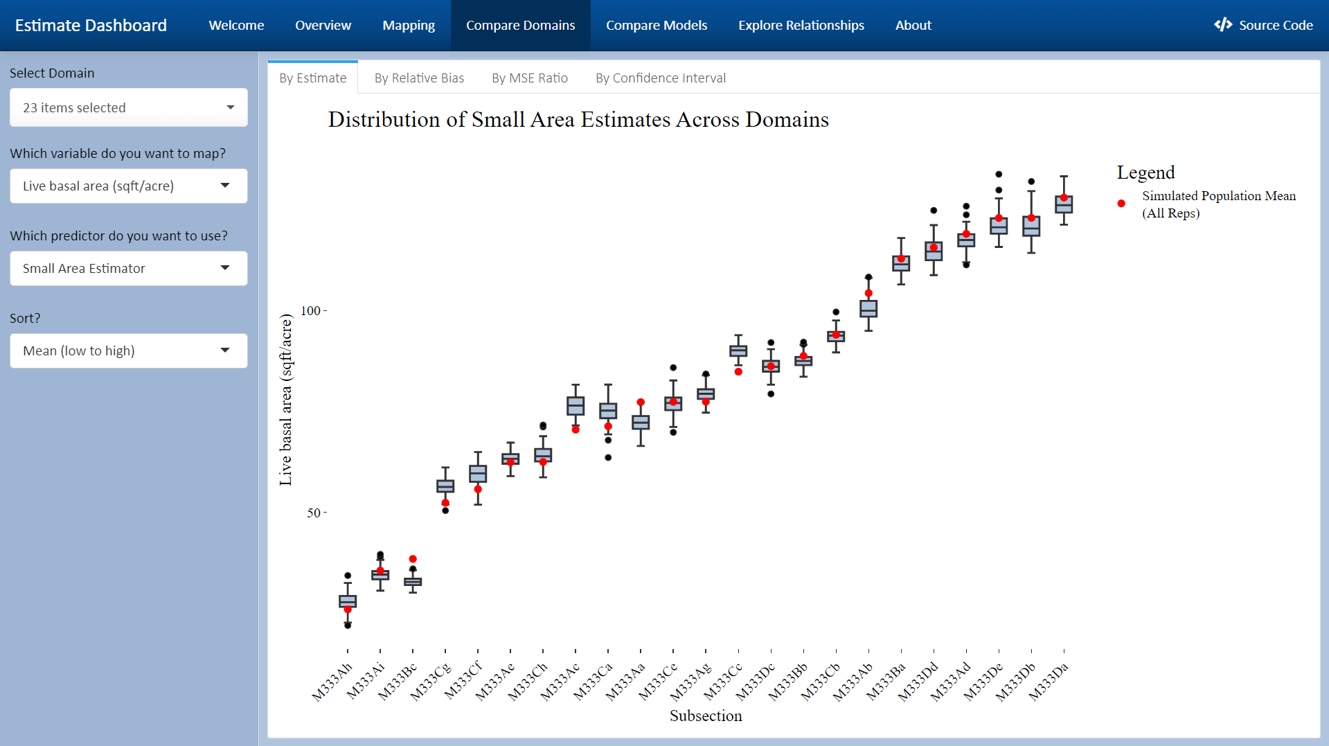
Figure 14: Screenshots of R Shiny app showing SAEs from a model with a bug in the code (above), and from the same model but with the bug fixed (below).

The app includes a “Compare Domains” page, in which the user can select one or more domains; a response variable; an estimator; and how to sort the domains. For these selections, boxplots for each of the 23 domains are used to show the distribution across 100 reps of estimates (Figure 14, lower subfigure), relative biases (Figure 15), MSE ratios (Figure 16), or CI coverages (Figure 17) on different tabs within the page. The next page is “Compare Models” (Figure 18), which is similar to “Compare Domains” except that it shows all three estimators for one domain, rather than multiple domains for one estimator.

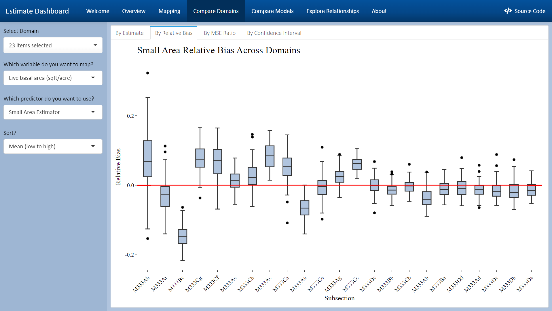
Figure 15: Screenshot of R Shiny app showing the relative biases of SAE models for Basal Area, for each of 23 domains. Each boxplot summarizes 100 reps.

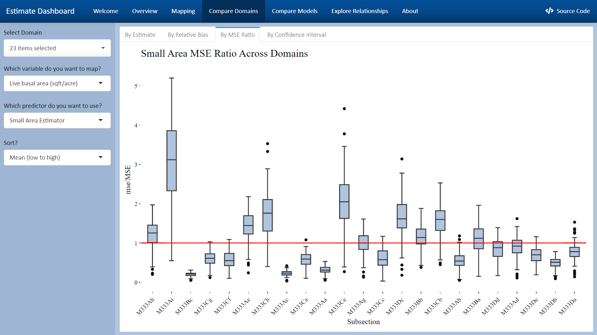
Figure 16: Screenshot of R Shiny app showing the $\widehat{\mbox{MSE}}/\mbox{MSE}$ ratios of SAE models for Basal Area, for each of 23 domains. Each boxplot summarizes 100 reps.

Figure 17: Screenshot of R Shiny app showing coverage of SAE models’ 95% confidence intervals for Basal Area, for each of 23 domains. Each bar summarizes 100 reps.

Finally, the “Explore Relationships” page (Figure 19) allows the user to view scatterplots of any response variable against any auxiliary variable, faceted into small multiples—one for each domain. This can be useful for model diagnostics: are there some auxiliary variables for which the unit-level models should differ substantially across domains?

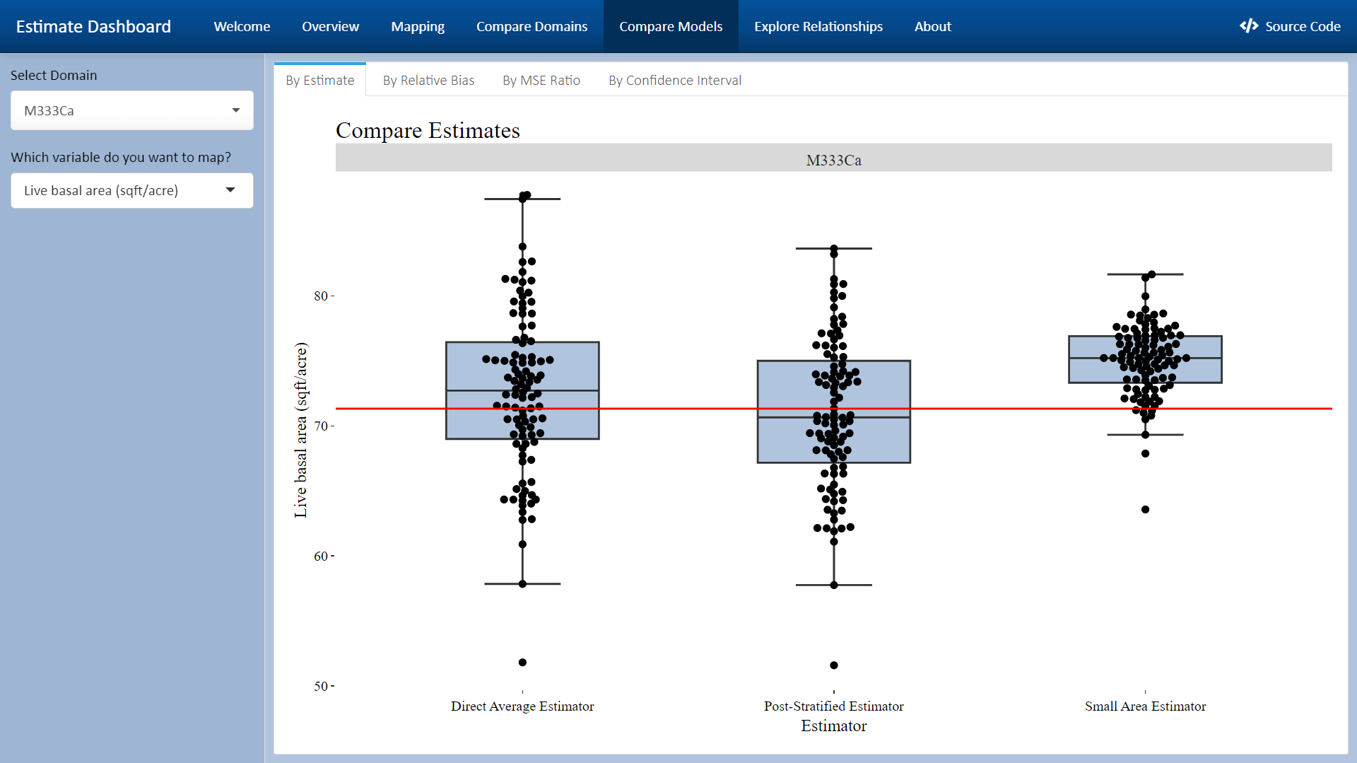
Figure 18: Screenshot of R Shiny app showing the estimates under three estimators for Basal Area, for one selected domain. Each boxplot summarizes 100 reps.

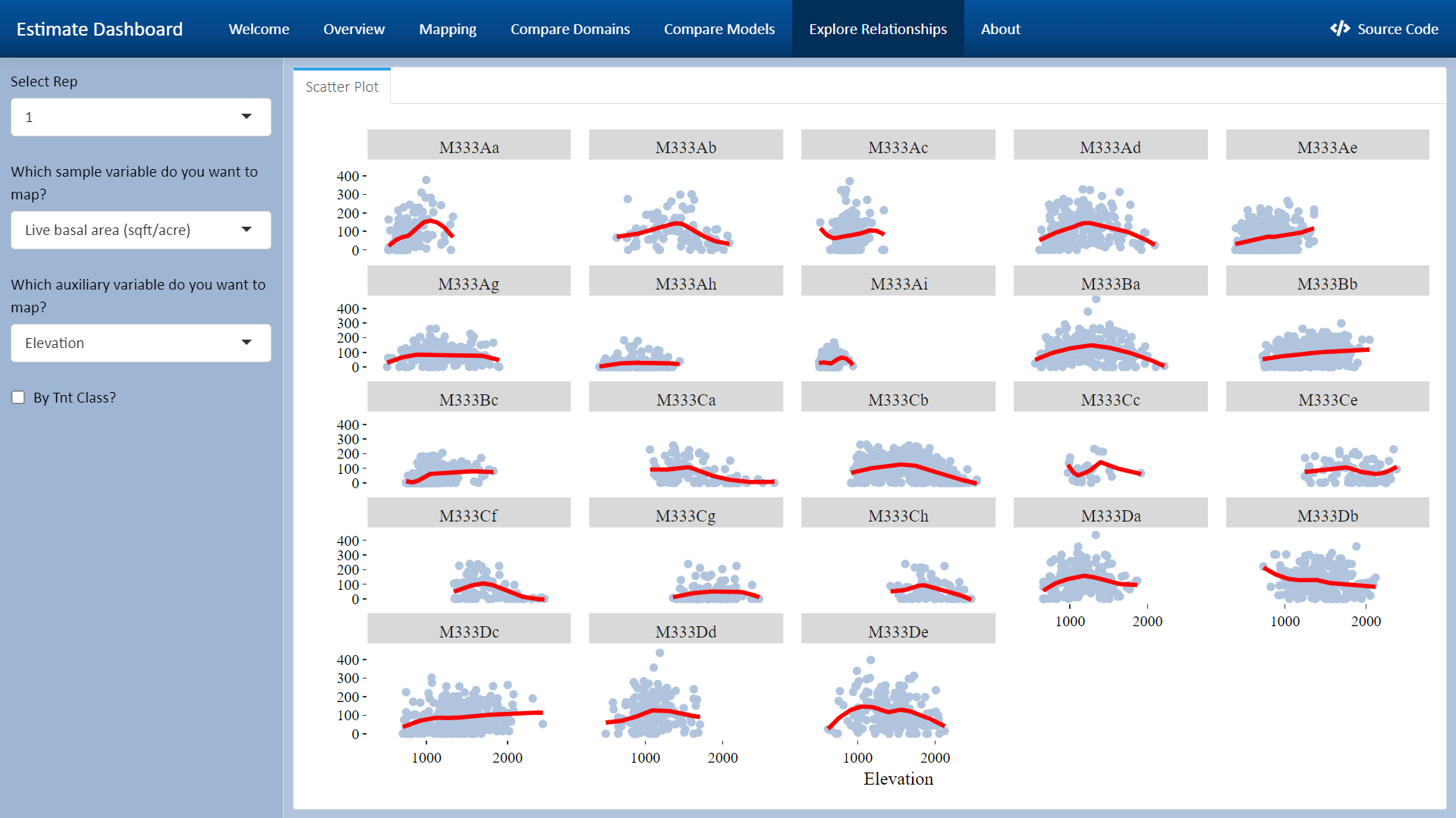
Figure 19: Screenshot of R Shiny app showing scatterplots of Basal Area against Elevation, for each of 23 domains, for sampled pixels in the first rep only.

We have also included a Mapping page (Figure 20), which shows a choropleth map of each domain’s estimates for a given estimator and rep. This allows users to see any spatial patterns that may be present in the estimates, as well as to explore how much these patterns vary across reps.

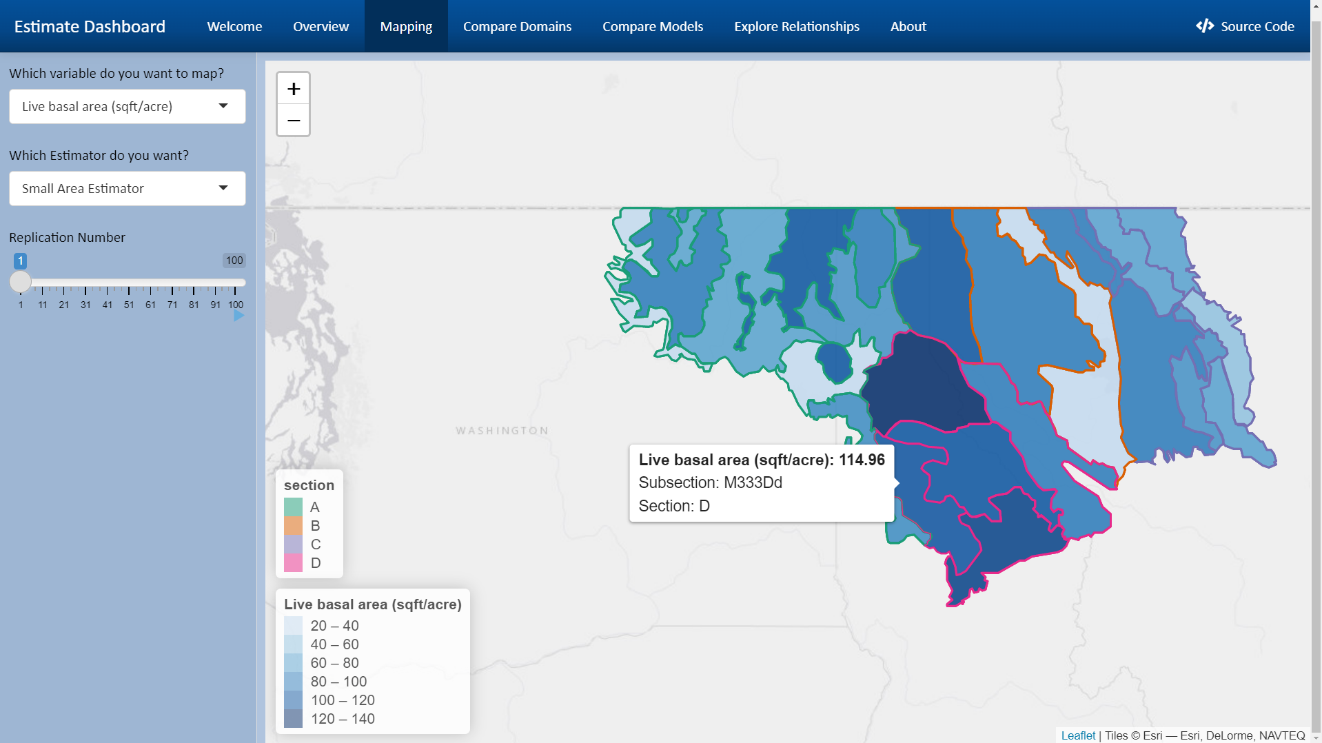
Figure 20: Screenshot of R Shiny app showing a choropleth map of SAE estimates for Basal Area for all of the 23 domains. One rep is selected, but the “Play” button can be used to start an animation to show the map for different reps.

We are currently using this R Shiny app to help us check and compare small area models ourselves. As we develop better models and concrete advice for users of SAEs for this population, we expect that the R Shiny app will also become useful for disseminating such advice to the diverse group of FIA users.

6 Discussion

We believe our kNN-based approximation to ABB works well here, where we have very rich and essentially complete auxiliary data for the entire population of interest. This is a different situation than in many demographic surveys, where we do not typically have auxiliary data for the entire human population of interest. Or if we do, it is not very rich: for instance, we might know a cross tabulation of counts of people by sex and race/ethnicity in each county, which can be converted into “complete auxiliary data”—but this is not rich enough X data to make precise matches using kNN. In such cases, the imputed Ys from KBAABB would not be much different than just using sampling weights to make multiple copies of the sample dataset.

One direction for future work is nonresponse. FIA surveys do experience some nonresponse (for instance, land owners may not admit a survey field crew, or weather conditions may make it impossible to visit a survey plot on schedule), though far less than a typical demographic survey and this nonresponse is usually treated as missing at random (MAR, [14]) within a given population [25]. So far, in generating and sampling from our artificial populations, we have assumed that nonresponse was missing completely at random (MCAR) and ignorable. However, in demographic applications we typically need to take extra care to ensure that imputation is used appropriately given what we know or posit about the nonresponse mechanism, which is often MAR or missing not at random (MNAR) rather than MCAR. Appropriate use of KBAABB for generating artificial populations when the survey data had non-MCAR nonresponse is an open question.

We have also not touched on a few complications specific to the FIA data, like subplots and condition classes or data vintage. Briefly, condition classes and subplots are more fine-grained levels of detail about the survey data collected at each plot. Our artificial population has been generated only at the plot level so far, and we may extend our methods to work at these other, smaller levels. Meanwhile, the issue of data vintage refers to accounting for the date at which each variable was measured. The survey data comes from a panel design, in which different plots are sampled in different years; and the surveyed pixels’ X variables may not be from the same year as the corresponding Y. Although most of the Xs change very slowly if at all from year to year (such as elevation or precipitation), others might be more timely (such as NDVI or EVI which should change as forests grow, become harvested, experience wildfires, etc.). Both our artificial population and our SAE models might benefit from using the right vintage of X to match the vintage of Y, though prior work by FIA researchers suggests that some common SAE models are fairly robust to data vintage in this population.

Aside from such details that are specific to our FIA data sources, we believe that KBAABB is a useful approach that could be widely applied to generate artificial populations and evaluate SAEs for any survey where rich, unit-level auxiliary data is available.

Appendix A Sensitivity to k

Besides KBAABB, we also tried to generate artificial populations by sampling uniformly from kNN with values of $k\in\{1,5,10,20,50,100\}$. We expected that $k$ of 10 or less might be reasonable, while much larger values would lead to artificial populations whose Y values were too close to being uniformly random, but we included larger $k$ values in order to check this. Indeed, results for KBAABB, $k$=1, and $k$=5 looked fairly similar, but $k$=10 or above were clearly less realistic. Among KBAABB, $k$=1, and $k$=5, the forestry subject-matter-expert on our team believed that KBAABB looks more realistic than $k$=1 or $k$=5, and the statisticians believed that KBAABB was better justified than $k$=1.

First we checked how $k$ affected the variability in imputed Y-values within each domain. Using BA (basal area) as an example, Figure 21 shows that for KBAABB as well as kNN with small values of $k$, each artificial population’s domain-level SDs are strongly but not perfectly correlated with their original-sample counterparts. As $k$ grows, we see the correlations get weaker, because for large $k$ we are drawing uniformly from a large donor pool where the donors do not necessarily resemble the recipient. Indeed, for large enough $k$ (larger than any shown here), we would simply be sampling donors uniformly from the whole sample and the scatterplot would be essentially horizontal.

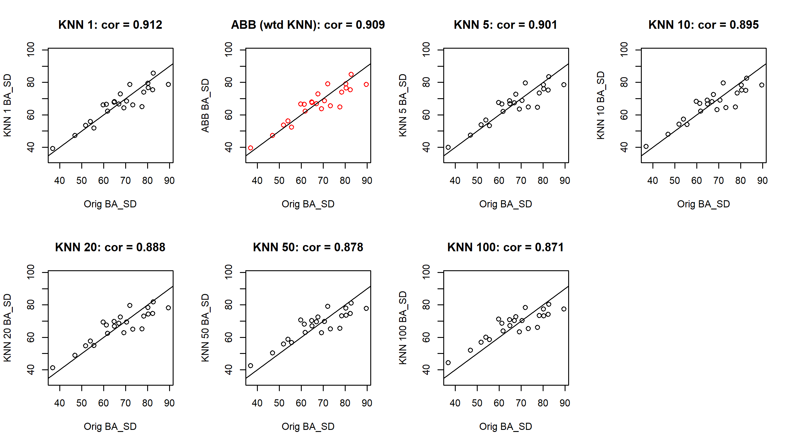
Figure 21: Original vs imputed SDs of BA (basal area) for each subsection, for KBAABB (red) and for kNN at several different $k$. All plots show $y=x$ line as a common reference.

Next, we checked the spatial smoothness of the imputed Y-variables, comparing kNN with various $k$ to the maps for KBAABB (Figure 6) and for X-variables (such as Figures 7 and 8). Spatial smoothness is not our primary goal because we are not yet attempting to fit spatial SAE models, though we may want to fit them in the future. However, we do want to have a realistic association between Ys and Xs at the unit level, and if the Xs are spatially smooth but the Ys were clearly not, that would indicate that we probably did not have a realistic association between Ys and Xs in our artificial population. The upper subfigure of Figure 22 shows kNN with $k$=1, which looks smoother than Figure 6 did, in the sense that there are many sizeable spatial regions of near-constant Y-values. However, for $k$=5 (lower subfigure of Figure 22) or greater (Figures 23 and 24), there is substantially more noise, in the sense that many pixels are quite likely to have individual spatial neighbors whose Y value is very far from their own. Although larger-scale spatial patterns can still be discerned in the plots for larger $k$, we deemed their lack of small-scale spatial smoothness to indicate unrealistic imputations.

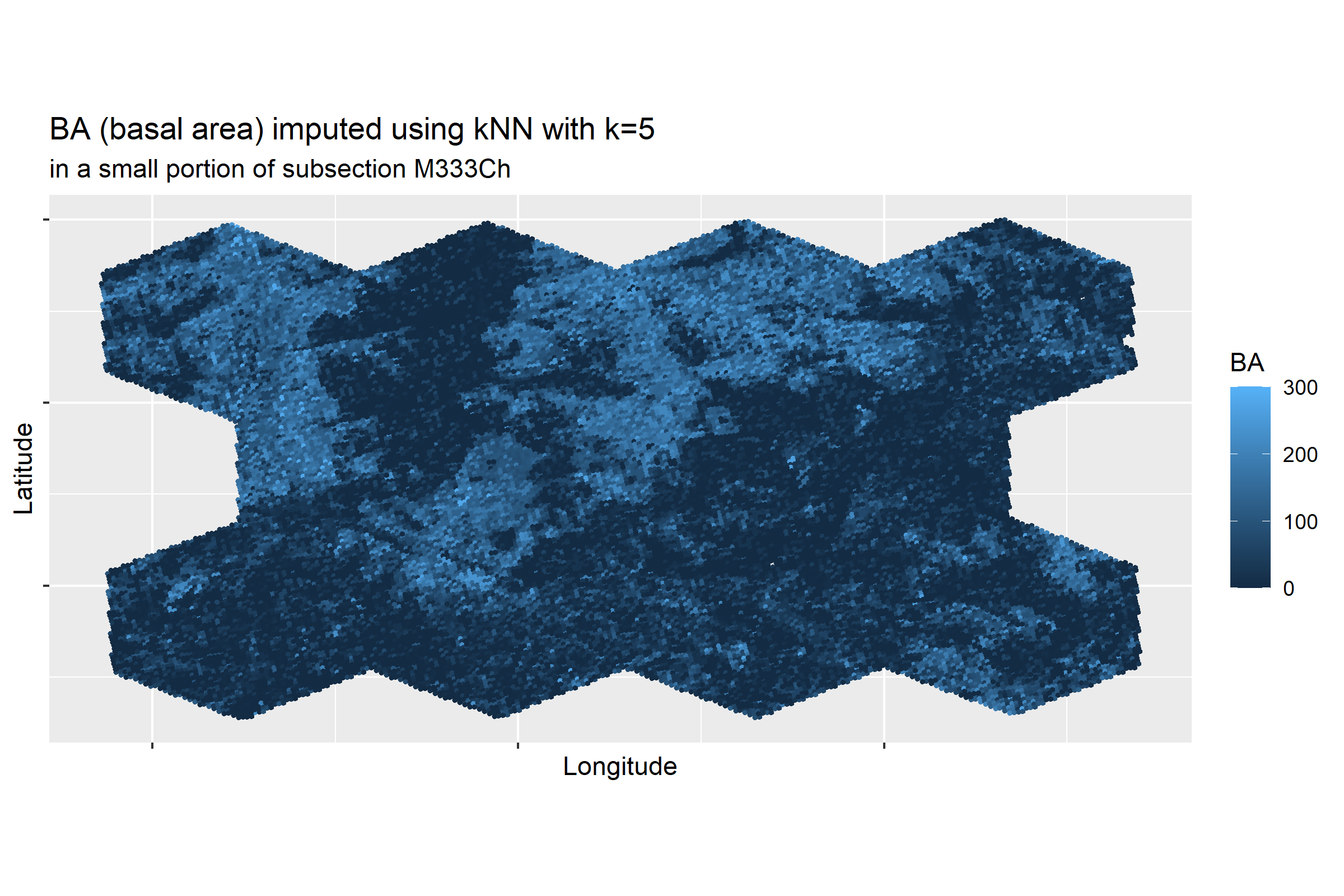
Figure 22: kNN with $k$=1 (above) and $k$=5 (below) imputations of BA (basal area) in a portion of subsection M333Ch.

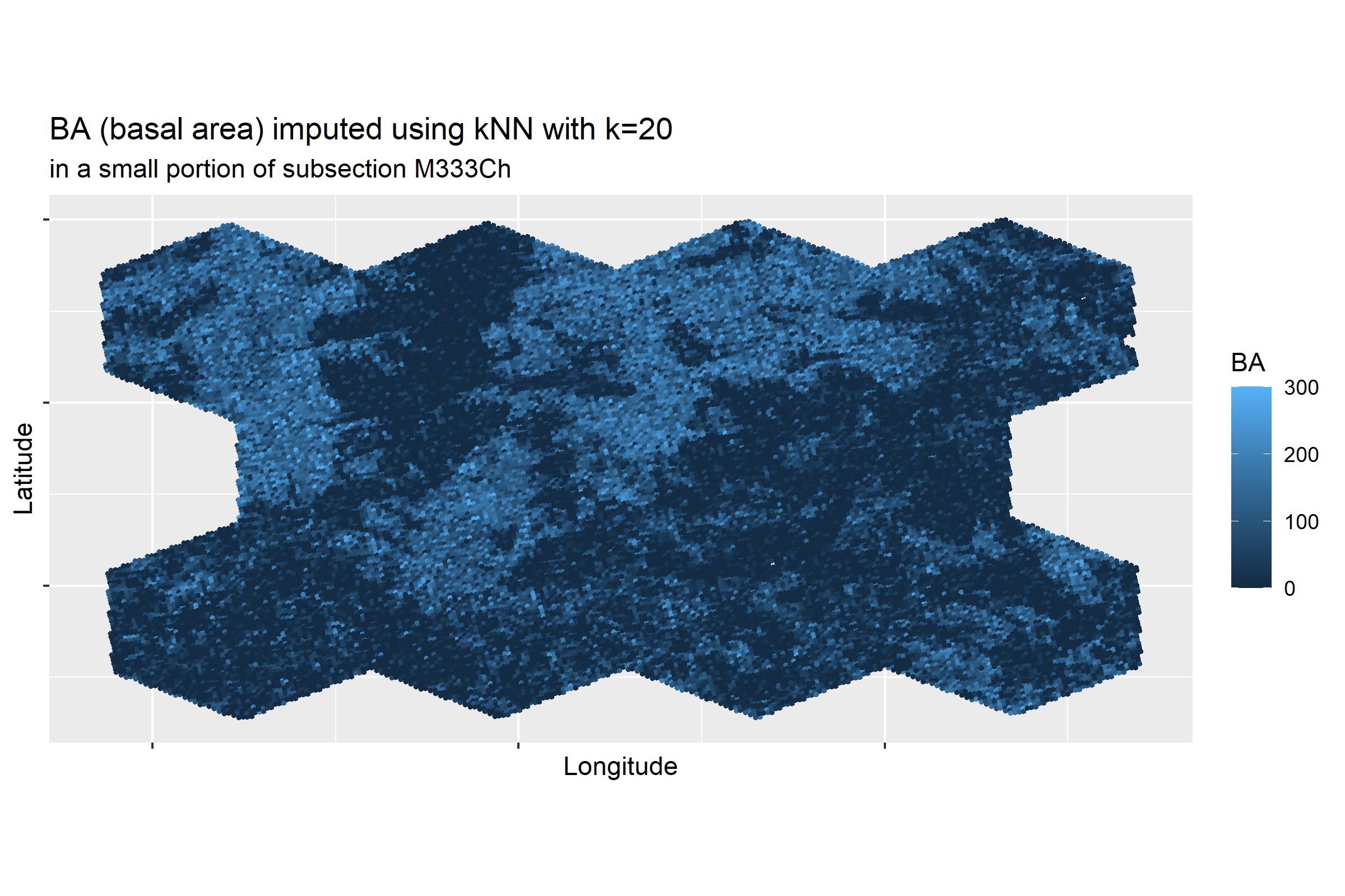
Figure 23: kNN with $k$=10 (above) and $k$=20 (below) imputations of BA (basal area) in a portion of subsection M333Ch.

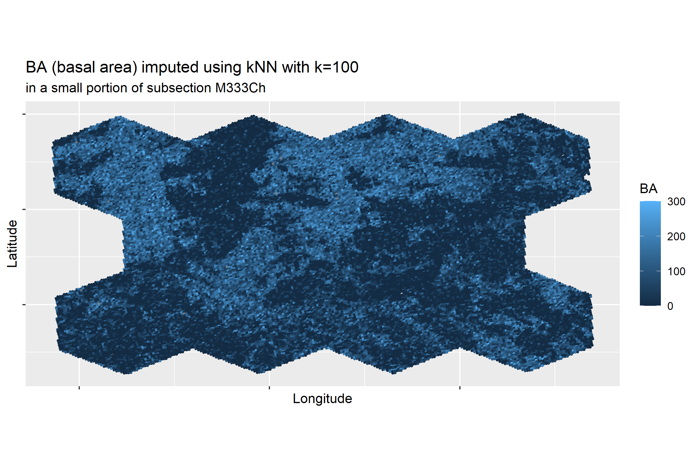
Figure 24: kNN with $k$=50 (above) and $k$=100 (below) imputations of BA (basal area) in a portion of subsection M333Ch.

References

- [1] “Agricultural Act of 2014”, 2014 URL: https://www.congress.gov/113/plaws/publ79/PLAW-113publ79.pdf
- [2] “Agriculture Improvement Act of 2018”, 2018 URL: https://www.agriculture.senate.gov/imo/media/doc/Agriculture%20Improvement%20Act%20of%202018.pdf
- [3] Gary Brown, Ray Chambers, Patrick Heady and Dick Heasman “Evaluation of small area estimation methods—an application to unemployment estimates from the UK LFS” In Proceedings of Statistics Canada Symposium 2001, 2001, pp. 1–10 Statistics Canada
- [4] John N K Rao and Isabel Molina “Small Area Estimation” John Wiley & Sons, 2015
- [5] Alan H Dorfman “Towards a routine external evaluation protocol for small area estimation” In International Statistical Review 86.2 Wiley Online Library, 2018, pp. 259–274
- [6] Nikos Tzavidis et al. “From start to finish: a framework for the production of small area official statistics” In Journal of the Royal Statistical Society, Series A (Statistics in Society) 181.4, 2018, pp. 927–979
- [7] Risto Lehtonen and Ari Veijanen “Design-based methods of estimation for domains and small areas” In Handbook of Statistics 29B Elsevier, 2009, pp. 219–249
- [8] Andreas Alfons, Stefan Kraft, Matthias Templ and Peter Filzmoser “Simulation of close-to-reality population data for household surveys with application to EU-SILC” In Statistical Methods & Applications 20.3 Springer, 2011, pp. 383–407
- [9] Jerzy Wieczorek, Ciara Nugent and Sam Hawala “A Bayesian zero-one inflated beta model for small area shrinkage estimation” In Proceedings of the 2012 Joint Statistical Meetings, American Statistical Association, Alexandria, VA, 2012
- [10] Jerzy Wieczorek and Carolina Franco “An Empirical Artificial Population and Sampling Design for Small-Area Model Evaluation” In Proceedings of the 2013 Joint Statistical Meetings, American Statistical Association, Alexandria, VA, 2013
- [11] Matthias Templ, Bernhard Meindl, Alexander Kowarik and Olivier Dupriez “Simulation of synthetic complex data: The R package simPop” In Journal of Statistical Software 79.10 UCLA, Dept. of Statistics, 2017, pp. 1–38
- [12] Donald B Rubin and Nathaniel Schenker “Multiple imputation for interval estimation from simple random samples with ignorable nonresponse” In Journal of the American Statistical Association 81.394 Taylor & Francis, 1986, pp. 366–374
- [13] Cary T Isaki and Wayne A Fuller “Survey design under the regression superpopulation model” In Journal of the American Statistical Association 77.377 Taylor & Francis, 1982, pp. 89–96
- [14] Donald B Rubin “Multiple imputation for nonresponse in surveys” John Wiley & Sons, 2004
- [15] Rebecca Roberts Andridge and Katherine Jenny Thompson “Adapting Nearest Neighbor for Multiple Imputation: Advantages, Challenges, and Drawbacks” In Journal of Survey Statistics and Methodology 11, 2023, pp. 213–233
- [16] George E Battese, Rachel M Harter and Wayne A Fuller “An error-components model for prediction of county crop areas using survey and satellite data” In Journal of the American Statistical Association 83.401 Taylor & Francis, 1988, pp. 28–36
- [17] Robert E Fay III and Roger A Herriot “Estimates of income for small places: an application of James-Stein procedures to census data” In Journal of the American Statistical Association 74.366a Taylor & Francis, 1979, pp. 269–277
- [18] Tim P Morris, Ian R White and Patrick Royston “Tuning multiple imputation by predictive mean matching and local residual draws” In BMC Medical Research Methodology 14.75 Springer, 2014, pp. 1–13
- [19] Rebecca R Andridge and Roderick JA Little “A review of hot deck imputation for survey non-response” In International Statistical Review 78.1 Wiley Online Library, 2010, pp. 40–64
- [20] Stephen Bates, Trevor Hastie and Robert Tibshirani “Cross-validation: what does it estimate and how well does it do it?” In arXiv preprint arXiv:2104.00673, 2021
- [21] Jerzy Wieczorek, Cole Guerin and Thomas McMahon “K-fold cross-validation for complex sample surveys” In Stat 11.1 Wiley Online Library, 2022, pp. e454
- [22] Nicholas L Crookston and Andrew O Finley “yaImpute: an R package for kNN imputation” In Journal of Statistical Software 23, 2008, pp. 1–16 URL: https://doi.org/10.18637/jss.v023.i10
- [23] Marcello D’Orazio “Integration and imputation of survey data in R: the StatMatch package” In Romanian Statistical Review 63.2 Romanian Statistical Review, 2015, pp. 57–68
- [24] Florian Meinfelder and Jannik Schaller “Data Fusion for Joining Income and Consumption Information using Different Donor-Recipient Distance Metrics” In Journal of Official Statistics 38.2, 2022, pp. 509–532
- [25] “The Enhanced Forest Inventory and Analysis Program—National Sampling Design and Estimation Procedures”, 2005
- [26] Donald B Rubin “Discussion: Statistical disclosure limitation” In Journal of Official Statistics 9.2 Statistics Sweden (SCB), 1993, pp. 461–468
- [27] Stephen E Fienberg, Udi E Makov and Russell J Steele “Disclosure limitation using perturbation and related methods for categorical data” In Journal of Official Statistics 14.4 Statistics Sweden (SCB), 1998, pp. 485–502
- [28] Jerome P Reiter “Satisfying disclosure restrictions with synthetic data sets” In Journal of Official Statistics 18.4 Statistics Sweden (SCB), 2002, pp. 531–543
- [29] EA Burrill et al. “The Forest Inventory and Analysis Database: Database Description and User Guide version 9.0.1 for Phase 2. USDA Forest Service”, 2021 URL: http://www.fia.fs.fed.us/library/database-documentation/
- [30] David T Cleland et al. “Ecological subregions: sections and subsections of the conterminous United States, presentation scale [1:3,500,000] [CD-ROM]”, 2007
- [31] ECOMAP “National hierarchical framework of ecological units”, 1993
- [32] Ronald E McRoberts et al. “The enhanced Forest Inventory and Analysis program of the USDA Forest Service: Historical perspective and announcement of statistical documentation” In Journal of Forestry 103.6 Oxford University Press, 2005, pp. 304–308
- [33] Linda S Heath et al. “Investigation into calculating tree biomass and carbon in the FIADB using a biomass expansion factor approach” In Proceedings of the Forest Inventory and Analysis (FIA) Symposium 2008, 2009, pp. 21–23
- [34] Patrick Schwager and Christian Berg “Remote sensing variables improve species distribution models for alpine plant species” In Basic and Applied Ecology 54 Elsevier, 2021, pp. 1–13
- [35] Kurtis J Nelson and Daniel Steinwand “A Landsat data tiling and compositing approach optimized for change detection in the conterminous United States” In Photogrammetric Engineering & Remote Sensing 81.7 Elsevier, 2015, pp. 573–586
- [36] “LANDFIRE: Landsat-derived indices”, 2016
- [37] “LANDFIRE Remap: improvements to Landsat image processing”, 2020 URL: https://www.landfire.gov/documents/LFRemap_ImageProcessing.pdf
- [38] Limin Yang et al. “A new generation of the United States National Land Cover Database: Requirements, research priorities, design, and implementation strategies” In ISPRS Journal of Photogrammetry and Remote Sensing 146 Elsevier, 2018, pp. 108–123
- [39] U.S. Geological Survey “LANDFIRE Elevation”, 2019
- [40] Christopher Daly et al. “A knowledge-based approach to the statistical mapping of climate” In Climate Research 22.2, 2002, pp. 99–113
- [41] Zachary A Holden et al. “TOPOFIRE: a topographically resolved wildfire danger and drought monitoring system for the conterminous United States” In Bulletin of the American Meteorological Society 100.9 American Meteorological Society, 2019, pp. 1607–1613
- [42] Daniele Zanaga et al. “ESA WorldCover 10 m 2020 v100” Zenodo, 2021
- [43] Matthew G Rollins “LANDFIRE: a nationally consistent vegetation, wildland fire, and fuel assessment” In International Journal of Wildland Fire 18.3 CSIRO Publishing, 2009, pp. 235–249
- [44] Joshua J Picotte et al. “LANDFIRE remap prototype mapping effort: Developing a new framework for mapping vegetation classification, change, and structure” In Fire 2.2 MDPI, 2019, pp. 35
- [45] Tracey Frescino and Grayson White “FIESTAnalysis: Analysis Functions for the FIESTA Package” R package version 0.2.1, 2022
- [46] TS Frescino et al. “FIESTA: A Forest Inventory Estimation and Analysis R Package” In Ecography Software Note, 2023 DOI: 10.1111/ecog.06428
- [47] Rebecca Andridge, Laura Bechtel and Katherine Jenny Thompson “Finding a flexible hot-deck imputation method for multinomial data” In Journal of Survey Statistics and Methodology 9.4 Oxford University Press, 2021, pp. 789–809
- [48] Lorenzo Beretta and Alessandro Santaniello “Nearest neighbor imputation algorithms: a critical evaluation” In BMC Medical Informatics and Decision Making 16.3 BioMed Central, 2016, pp. 197–208
- [49] Andrew Gelman, Xiao-Li Meng and Hal Stern “Posterior predictive assessment of model fitness via realized discrepancies” In Statistica Sinica 6, 1996, pp. 733–760
- [50] Gareth James, Daniela Witten, Trevor Hastie and Robert Tibshirani “An Introduction to Statistical Learning with Applications in R” Springer, 2021
- [51] Shu Yang and Jae Kwang Kim “Nearest neighbor imputation for general parameter estimation in survey sampling” In The Econometrics of Complex Survey Data 39 Emerald Publishing Limited, 2019, pp. 209–234
- [52] Jared S Murray “Multiple Imputation: A Review of Practical and Theoretical Findings” In Statistical Science 33.2, 2018, pp. 142–159
- [53] Jiahua Chen and Jun Shao “Nearest neighbor imputation for survey data” In Journal of Official Statistics 16.2 Statistics Sweden (SCB), 2000, pp. 113
- [54] Michael W Robbins “The utility of nonparametric transformations for imputation of survey data” In Journal of Official Statistics 30.4, 2014, pp. 675–700
- [55] Shengqiao Li “FNN: Fast Nearest Neighbor Search Algorithms and Applications” R package version 1.1.3.1, 2019 URL: https://CRAN.R-project.org/package=FNN
- [56] U A M Nur, N T Longford, J E Cade and D C Greenwood “Dealing with incomplete data in questionnaires of food and alcohol consumption” In Statistics in Transition 7.1 Polish Statistical Association, 2005, pp. 111–134
- [57] Federica Baffetta, Lorenzo Fattorini, Sara Franceschi and Piermaria Corona “Design-based approach to k-nearest neighbours technique for coupling field and remotely sensed data in forest surveys” In Remote Sensing of Environment 113.3 Elsevier, 2009, pp. 463–475
- [58] D.. Horvitz and D.. Thompson “A generalization of sampling without replacement from a finite universe” In Journal of the American Statistical Association 47, 1952, pp. 663–685
- [59] Ralph S Woodruff “Use of a regression technique to produce area breakdowns of the monthly national estimates of retail trade” In Journal of the American Statistical Association 61.314 Taylor & Francis, 1966, pp. 496–504
- [60] Olek C Wojcik et al. “GREGORY: A Modified Generalized Regression Estimator Approach to Estimating Forest Attributes in the Interior Western US” In Frontiers in Forests and Global Change 4 Frontiers, 2022
- [61] TS Frescino, C Toney and GW White “FIESTAutils: Utility Functions for Forest Inventory Estimation and Analysis” R package version 1.1.5, 2023 URL: https://CRAN.R-project.org/package=FIESTAutils
- [62] Winston Chang et al. “shiny: Web Application Framework for R” R package version 1.7.3, 2022 URL: https://CRAN.R-project.org/package=shiny