Gyrokinetic theory of toroidal Alfvén eigenmode saturation via nonlinear wave-wave coupling

Abstract

Nonlinear wave-wave coupling constitutes an important route for the turbulence spectrum evolution in both space and laboratory plasmas. For example, in a reactor relevant fusion plasma, a rich spectrum of symmetry breaking shear Alfvén wave (SAW) instabilities are expected to be excited by energetic fusion alpha particles, and self-consistently determine the anomalous alpha particle transport rate by the saturated electromagnetic perturbations. In this work, we will show that the nonlinear gyrokinetic theory is a necessary and powerful tool in qualitatively and quantitatively investigating the nonlinear wave-wave coupling processes. More specifically, one needs to employ the gyrokinetic approach in order to account for the breaking of the “pure Alfvénic state" in the short wavelength kinetic regime, due to the short wavelength structures associated with nonuniformity intrinsic to magnetically confined plasmas.

Using well-known toroidal Alfvén eigenmode (TAE) as a paradigm case, three nonlinear wave-wave coupling channels expected to significantly influence the TAE nonlinear dynamics are investigated to demonstrate the strength and necessity of nonlinear gyrokinetic theory in predicting crucial processes in a future reactor burning plasma. These are: 1. the nonlinear excitation of meso-scale zonal field structures via modulational instability and TAE scattering into short-wavelength stable domain; 2. the TAE frequency cascading due to nonlinear ion induced scattering and the resulting saturated TAE spectrum; and 3. the cross-scale coupling of TAE with micro-scale ambient drift wave turbulence and its effect on TAE regulation and anomalous electron heating.

1 Introduction

Shear Alfvén waves (SAWs) HAlfvenNature1942 are fundamental electromagnetic fluctuations in magnetised plasmas, and are ubiquitous in space and laboratories. SAWs exist due to the balance of restoring force due to magnetic field line bending and plasma inertia, and are characterized by transverse magnetic perturbations propagating along equilibrium magnetic field lines, with the parallel wavelength comparable to system size, while perpendicular wavelength varying from system size to ion Larmor radius. Due to their incompressible character, SAWs can be driven unstable with a lower threshold in comparison to that of compressional Alfvén waves or ion acoustic waves. In magnetically confined plasmas typical of fusion reactors such as ITER KTomabechiNF1991 and CFETR YWanNF2017 , with their phase/group velocity comparable to the characteristic speed of super-thermal fusion alpha particles, SAW instabilities could be strongly excited by fusion alpha particles as well as energetic particles (EPs) from auxiliary heating. The enhanced symmetry-breaking SAW fluctuations could lead to transport loss of EPs across magnetic field surfaces; raising an important challenge to the good EP confinement required for sustained burning AFasoliNF2007 ; LChenRMP2016 .

In magnetic confined fusion devices, due to the nonuniformities associated with equilibrium magnetic geometry and plasma profile, SAW frequency varies continuously across the magnetic surfaces and forms a continuous spectrum HGradPT1969 , on which SAWs suffer continuum damping by mode conversion to small scale structures Landau damped, predominantly, by electrons LChenPoF1974 ; AHasegawaPoF1976 ; LChenRMPP2021 . As a result, SAW instabilities can be excited as various kinds of EP continuum modes (EPMs) when the EP resonant drive overcomes continuum damping LChenPoP1994 , or as discretised Alfvén eigenmodes (AEs) inside continuum gaps to minimise the continuum damping, among which, the famous toroidal Alfvén eigenmode (TAE) CZChengAP1985 ; LChenVarenna1988 ; GFuPoFB1989 ; KWongPRL1991 is a celebrated example. For a thorough understanding of the SAW instability spectrum in reactors, interested readers may refer to Refs. GVladRNC1999 ; AFasoliNF2007 ; FZoncaPoP2014b ; LChenRMP2016 ; YTodoRMPP2019 for comprehensive reviews.

The SAW instability induced EP anomalous transport/acceleration/heating rate, depends on the SAW instability amplitude and spectrum via wave-particle resonance conditions LChenJGR1999 ; LChenJGR1991 , which are, determined by the nonlinear saturation mechanisms. The first channel for SAW instability nonlinear saturation is the nonlinear wave-particle interactions, i.e., the acceleration/deceleration of EPs by SAW instability induced EP “equilibrium" distribution function evolution and the consequent self-consistent SAW spectrum evolution, among which there are well-known and broadly used models introduced by Berk et al HBerkPoFB1990a ; HBerkPoFB1990b ; HBerkPoFB1990c by analogy to the wave-particle trapping in one-dimensional beam-plasma instability system TOneilPoF1965 . More recently, Zonca et al systematically developed the non-adiabatic wave-particle interaction theory, based on nonlinear evolution of phase space zonal structures (PSZS) FZoncaJPCS2021 ; FZoncaNJP2015 ; MFalessiPoP2019 ; MFalessiNJP2023 ; FZoncaPPCF2015 , i.e., the phase space structures that are un-damped by collisionless processes. The PSZS approach, by definition of the “renormalised" nonlinear equilibria typically varying on the mesoscales in the presence of microscopic turbulences, self-consistently describes the EP phase space non-adiabatic evolution and nonlinear evolution of turbulence due to varying EP “equilibrium" distribution function, very often in the form of non-adiabatic frequency chirping, and is described by a closed Dyson-Schr$\ddot{o}$dinger model FZoncaJPCS2021 . Both processes are tested and corresponding theoretical frameworks are broadly used in interpretation of experimental results as well as large scale numerical simulations, e.g., XWangPRE2012 ; HZhangPRL2012 ; LYuEPL2022 . The other channel for SAW nonlinear evolution, relatively less explored in large-scale simulations, is the nonlinear wave-wave coupling mechanism, describing SAW instability spectrum evolution due to interaction with other electromagnetic oscillations, and is the focus of the present brief review using TAE as a paradigm case. These approaches developed for TAE and the obtained results, are general, and can be applied to other SAW instabilities based on the knowledge of their linear properties.

The nonlinear wave-wave coupling process, as an important route for SAW instability nonlinear dynamic evolution and saturation LChenPoP2013 , is expected to be even more important in burning plasmas of future reactors; where, different from present-day existing magnetically confined devices, the EP power density can be comparable with that of bulk thermal plasmas, and the EP characteristic orbit size is much smaller than the system size. As a consequence, there is a rich spectrum of SAW instabilities in future reactors AFasoliNF2007 ; LChenRMP2016 ; TWangPoP2018 ; ZRenNF2020 , with most unstable modes being characterized by $n\gtrsim O(10)$ for maximized wave-particle power exchange, with $n$ being the toroidal mode number. That is, multi-$n$ modes with comparable linear growth rates could be excited simultaneously. These SAW instabilities are, thus, expected to interact with each other, leading to complex spectrum evolution that eventually affects the EP transport. It is noteworthy that the nonlinear wave-particle interaction, described by Dyson Schr$\ddot{o}$dinger model and nonlinear wave-wave couplings embedded within a generalized nonlinear Schr$\ddot{o}$dinger equation, are two pillars of the unified theoretical framework for self-consistent SAW nonlinear evolution and EP transport, as summarized in Ref. FZoncaJPCS2021 , which is being actively developed by the Center for Nonlinear Plasma Physics (CNPS) collaboration .

Due to the typically short scale structures associated with continuous spectrum, the nonlinear couplings of SAW instabilities are dominated by the perpendicular nonlinear scattering via Reynolds and Maxwell stresses, instead of the polarization nonlinearity AHasegawaPoF1976 ; LChenEPL2011 ; RSagdeevbook1969 . Thus, the kinetic treatment is needed to capture the essential ingredients of SAW nonlinear wave-wave coupling dominated by small structures that naturally occur due to SAW continuum, and some other fundamental physics not included in magnetohydrodynamic (MHD) theory, e.g., the wave-particle interaction crucial for ion induced scattering of TAEs TSHahmPRL1995 ; ZQiuNF2019a , and trapped particle effects in the low frequency range that may lead to neoclassical inertial enhancement, which plays a key role for zonal field structure (ZFS) generation MRosenbluthPRL1998 ; LChenPoP2000 ; LChenPRL2012 . These crucial physics ingredients are not included in the MHD description, and kinetic treatment is mandatory to both quantitatively and qualitatively study the nonlinear wave-wave coupling processes of SAWs. These features can be fully and conveniently covered by nonlinear gyrokinetic theory EFriemanPoF1982 derived by systematic removal of fast gyro motions with $\Omega_{c}\gg\omega_{A}$, and yield quantitatively, using TAE as a paradigm case, the nonlinear saturation level and corresponding EP transport and/or heating. The general knowledge obtained here, as noted in the context of this review, can be straightforwardly applied to other kinds of SAW instabilities, with the knowledge of their linear properties.

The rest of the paper is organized as follows. In Sec. 2, the general background knowledge of nonlinear wave-wave coupling of SAW instabilities in toroidal geometry are introduced, where SAW instabilities in toroidal plasmas and nonlinear wave-wave coupling are briefly reviewed. The kinetic theories of TAE saturation via nonlinear wave-wave coupling are reviewed in Sec. 3, where three channels for TAE nonlinear dynamic evolution are introduced. Finally, a brief summary is given in Sec. 4.

2 Theoretical framework of nonlinear mode coupling and SAWs in toroidal plasmas

In this section, the basic elements needed for SAW nonlinear mode coupling are introduced, including the linear SAW dispersion relation, pure Alfvénic state, perpendicular nonlinear coupling, and nonlinear gyrokinetic theoretical framework. For accessibility to general readers, these materials are introduced in a pedagogical way. Readers interested in more technical details may refer to references given.

2.1 Nonlinear wave-wave coupling

The nonlinear wave-wave coupling corresponds to wave spectrum evolution due to interaction with other collective oscillations, and is an important pillar of nonlinear plasma physics RSagdeevbook1969 . For SAW instability, there is an important property that, in uniform plasmas and ideal MHD limit, the Reynolds and Maxwell stresses, will exactly cancel each other. Thus, SAWs can grow to large amplitudes without being distorted by nonlinear effects. This is called “pure Alfvénic state", and will be addressed briefly below. As a result, for the nonlinear mode couplings of SAWs, the pure Alfvénic state shall be broken by, e.g., system nonuniformity and/or kinetic compression, as addressed in Ref. LChenPoP2013 .

The momentum equation for the incompressible SAW nonlinear evolution in the low $\beta$ plasma limit, keeping up to quadratic terms, can be written as

$$\rho_{0}(\partial_{t}+\delta\mathbf{v}\cdot\nabla)\delta\mathbf{v}=\delta\mathbf{J}\times\mathbf{B}_{0}/c+\delta\mathbf{J}\times\delta\mathbf{B}/c,$$ (1)

with $\rho$ being the mass density, $\mathbf{v}$ the fluid velocity, $\mathbf{J}$ the current density, $\mathbf{B}$ the magnetic field, and $\delta$ indicating perturbed quantities. Equation (1), together with the Ampere’s law

$$\nabla\times\delta\mathbf{B}=4\pi\delta\mathbf{J}/c$$ (2)

and the Faraday’s law with ideal MHD condition embedded,

$$\partial_{t}\delta\mathbf{B}=\nabla\times(\delta\mathbf{v}\times\mathbf{B}_{0}),$$ (3)

yield, in the linear limit,

$$\frac{\delta\mathbf{v}}{V_{A}}=\pm\frac{\delta\mathbf{B}}{B_{0}},$$ (4)

which correspond to the famous Walen relation CKierasJPP1982 . In deriving equation (4), the linear SAW dispersion relation, derived from linearised equations (1) and (3), $\omega^{2}=k^{2}_{\parallel}V^{2}_{A}$ is used, with $V_{A}\equiv\sqrt{B^{2}_{0}/(4\pi\rho_{0})}$ being the Alfvén velocity.

Equation (1), in the nonlinear limit, can be re-written as

$$\rho_{0}\partial_{t}\delta\mathbf{v}^{(2)}=-\nabla\lvert\delta B\rvert^{2}/(8\pi)-\mbox{MX}-\mbox{RS},$$ (5)

with $\mbox{MX}\simeq-\delta\mathbf{B}_{\perp}\cdot\nabla\delta\mathbf{B}_{\perp}/(4\pi)$ and $\mbox{RS}\equiv\rho_{0}\delta\mathbf{v}_{\perp}\cdot\nabla\delta\mathbf{v}_{\perp}$ being, respectively, the Maxwell and Reynolds stresses, and the first term on the right hand side corresponding to the parallel ponderomotive force RSagdeevbook1969 , which is typically much smaller than RS and MX due to the typical $k_{\parallel}\ll k_{\perp}$ ordering. It can be seen clearly that, in the present model of ideal MHD, uniform plasma limit, RS and MX cancel each other, so SAW can grow to large amplitude without being distorted by nonlinear processes. Thus, to understand the nonlinear evolution of SAW instabilities as this pure Alfvénic state is broken, higher order nonlinearities that occur on longer time scales should be introduced; i.e., it is necessary to go beyond the ideal MHD description. As we shall show in the following applications using TAE as an example, plasma nonuniformity as well as plasma compressibility may play crucial roles in breaking the Alfvénic state for different control parameters. In order to account for these effects for SAWs as well as drift waves (DWs) involved in the analysis with frequencies much lower than ion cyclotron frequency, nonlinear gyrokinetic theory is shown to be extremely useful in studying the nonlinear wave-wave interaction physics, and is introduced in the Sec. 2.2. For a thorough discussion of pure Alfvénic state and SAW/KAW nonlinear dynamics as it is broken by various effects, interested readers may refer to Ref. LChenPoP2013 for more details.

2.2 Nonlinear gyrokinetic theoretical framework

The nonlinear gyrokinetic equation is derived by systematic removal of the fast gyro-motion of particles, noting the conservation of magnetic moment $\mu\equiv mv^{2}_{\perp}/(2B)$ in the low frequency regime with $\omega\ll\Omega_{c}$, and it is a powerful tool in theoretical/numerical studies of low frequency fluctuations of interest in magetically confined plasmas EFriemanPoF1982 ; ABrizardRMP2007 ; HSugamaRMPP2017 . In gyrokinetic theory, the fluctuating particle response can be separated into adiabatic and non-adiabatic components,

$$\delta f_{j}=\left(\frac{q}{m}\right)_{j}\delta\phi_{k}\frac{\partial}{\partial E}F_{0j}+\exp(-\mathbf{\rho}\cdot\nabla)\delta H_{j},$$ (6)

with the non-adiabatic particle response derived from nonlinear gyrokinetic equation EFriemanPoF1982

$$\left(\partial_{t}+v_{\parallel}\mathbf{b}\cdot\nabla+\mathbf{v}_{d}\cdot\nabla\right)\delta H_{k}$$ (7)

$$= i\frac{q}{m}\left(\omega\partial_{E}+\hat{\omega}_{*}\right)F_{0}J_{k}\delta L_{k}-\sum_{\mathbf{k}=\mathbf{k}^{\prime}+\mathbf{k}^{\prime\prime}}\Lambda^{k^{\prime}}_{k^{\prime\prime}}J_{k^{\prime}}\delta L_{k^{\prime}}\delta H_{k^{\prime\prime}}.$$

Here, $E=v^{2}/2$ is the energy per unit mass, $\mathbf{v}_{d}=\mathbf{b}\times[(v^{2}_{\perp}/2)\nabla\ln B_{0}+v^{2}_{\parallel}\mathbf{b}\cdot\nabla\mathbf{b}]$ is the magnetic drift, $\hat{\omega}_{*}\equiv\mathbf{k}\cdot\mathbf{b}\times\nabla\ln{F_{0}}/\Omega_{c}$ is related to the diamagnetic drift frequency associated with plasma nonuniformities. In the present work focusing on the nonlinear evolution of TAE with prescribed amplitude due to nonlinear mode coupling, with dominant role played by thermal plasma contribution to RS and MX , in the rest of the manuscript, Maxwellian distribution function is adopted for thermal plasmas, and one has $\partial_{E}F_{M}=-(m/T)F_{M}$, $\hat{\omega}_{*}F_{M}=(m/T)\omega_{*}F_{M}$ with $\omega_{*}\equiv-i(cT/qB_{0})_{j}\mathbf{b}\times\nabla\ln F_{M}\cdot\nabla=ck_{\theta}T_{j}/(qB_{0}L_{n})_{j}\left[1+\eta(E/T-3/2)\right]_{j}$, $k_{\theta}$ is the poloidal wavenumber, and $\eta=L_{n}/L_{T}$ with $L_{n}$ and $L_{T}$ being respectively the characteristic scale length of density and temperature nonuniformities. Furthermore, $J_{k}\equiv J_{0}(k_{\perp}\rho)$ is the Bessel function of zero-index accounting for finite Larmor radius effects, $\delta L_{k}\equiv\delta\phi-v_{\parallel}\delta A_{\parallel}/c$, and $\Lambda^{k^{\prime}}_{k^{\prime\prime}}\equiv(c/B_{0})\mathbf{b}\cdot\mathbf{k^{\prime\prime}}\times\mathbf{k^{\prime}}$ accounts for perpendicular scattering with the constraint on wavenumber matching condition given by $\mathbf{k}=\mathbf{k}^{\prime}+\mathbf{k}^{\prime\prime}$. In the rest of the paper, $-i\partial_{l}\delta\psi_{k}=\omega\delta A_{\parallel k}/c$ is introduced for conveniently treating the inductive parallel electric field component, which allows recovering the ideal MHD condition ($\delta E_{\parallel}=0$) by straightforwardly taking $\delta\psi_{k}=\delta\phi_{k}$.

The governing equations are derived from quasi-neutrality condition

$$\frac{n_{0}e^{2}}{T_{i}}\left(1+\frac{T_{e}}{T_{i}}\right)\delta\phi_{k}=\sum_{j=e,i}\left\langle qJ_{k}\delta H_{k}\right\rangle,$$ (8)

with angular brackets denoting velocity space integration and, with magnetic compression being negligible in the low-$\beta$ limit of interest here, the nonlinear gyrokinetic vorticity equation becomes LChenJGR1991 ; LChenNF2001

$$\frac{c^{2}}{4\pi\omega^{2}}B\frac{\partial}{\partial l}\frac{k^{2}_{\perp}}{B}\frac{\partial}{\partial l}\delta\psi_{k}+\frac{e^{2}}{T_{i}}\left(1-\frac{\omega_{*}}{\omega}\right)_{k}\left\langle\left(1-J^{2}_{k}\right)F_{M}\right\rangle\delta\phi_{k}-\sum_{j=e,i}\left\langle qJ_{0}\frac{\omega_{d}}{\omega}\delta H\right\rangle_{k}$$ (9)

$$= -\frac{i}{\omega_{k}}\sum_{\mathbf{k}=\mathbf{k}^{\prime}+\mathbf{k}^{\prime\prime}}\Lambda^{k^{\prime}}_{k^{\prime\prime}}\left[\left\langle e(J_{k}J_{k^{\prime}}-J_{k^{\prime\prime}})\delta L_{k^{\prime}}\delta H_{k^{\prime\prime}}\right\rangle+\frac{c^{2}}{4\pi}k^{\prime\prime 2}_{\perp}\frac{\partial_{l}\delta\psi_{k^{\prime}}\partial_{l}\delta\psi_{k^{\prime\prime}}}{\omega_{k^{\prime}}\omega_{k^{\prime\prime}}}\right].$$

Nonlinear gyrokinetic vorticity equation is derived from parallel Ampere’s law, quasi-neutrality condition and nonlinear gyrokinetic equation, and it forms, together with quasi-neutrality condition, equation (8), a closed set of equations describing the dynamics of low frequency fluctuations in low $\beta$ plasmas. Note that, for the application in the present review, in equation (9), only effects associated with plasma density nonuniformity are accounted for, while effects associated with temperature gradients are neglected systematically, i.e., $\eta\equiv L_{n}/L_{T}=0$. The terms on the left hand side of equation (9) are, respectively, the field line bending, inertia and curvature-pressure coupling terms. This clearly shows the convenience of the present formulation based on the gyrokinetic vorticity equation in studying SAW related physics, since field bending and inertia terms balance at the leading order for these fluctuations. The terms on the right hand side, on the other hand, are the formally nonlinear generalized gyrokinetic RS and MX, dominated, respectively, by ion and electron contributions.

In this brief review focusing on the TAE physics due to nonlinear wave-wave interactions, TAE with prescribed amplitude are assumed, while EPs contribution is typically small. Thus, we include only the thermal plasma contribution in the above governing equations. The EPs, crucial for the TAE excitation, can also be important in ZFS generation during the TAE exponential growth phase due to resonant EP drive. This interesting topic of nonlinear ZFS forced driven process connected with the nonlinear EP response is beyond the scope of the present review and will only be briefly discussed in Sec. 3.1.

Note that, for TAE of interest of the present review, with frequency typically much larger than thermal plasma diamagnetic frequency, the system nonuniformity associated with $\omega_{*}$ is typically weak and, thus, systematically neglected in the majority of present review on TAE nonlinear physics. It is maintained, however, in Sec. 3.3 in the analysis of TAE scattering by DWs, where finite $\omega_{*}$ is crucial for the high-n DW physics, as well as for the enhancement of nonlinear scattering rates due to the $\lvert\omega_{*}\rvert\gg\lvert v_{i}/(qR_{0})\rvert$ ordering.

2.3 SAW instabilities in toroidal plasmas

In this section, the SAW dispersion relation in the WKB limit will be derived, which is then used to symbolically demonstrate the formation of SAW continuum structure and the existence of discrete Alfvén eigenmode, using the well-known TAE as an example. The obtained linear particle responses can be used in the following analysis of TAE nonlinear dynamics via nonlinear wave-wave coupling processes. For the convenience of following analysis on nonlinear wave-wave couplings, the particle responses to SAW, are derived in real space, and the obtained mode equation, will be solved by transforming into ballooning space. Note that for TAE of interest here, $\lvert\omega_{*}/\omega\rvert\ll 1$ is satisfied for most unstable TAEs with perpendicular wavelength comparable to EP drift orbit width; so that the thermal plasma $\omega_{*}$ effects on SAW dispersion relation are expected to be small. Thus, in the majority of the paper, the $\omega_{*}$ effects on TAE/KAW dispersion relation are systematically neglected. However, in our derivation of linear thermal plasma response to SAW $\omega_{*}$ correction is kept, which will be used in Sec. 3.3, where $\omega_{*}$ effects on KAW can be important due to its relatively high toroidal mode number due to momentum conservation in high-n DW scattering.

The linear electron response to SAW can be derived noting the $\lvert\omega/k_{\parallel}v_{e}\rvert\ll 1$ ordering, and one obtains

$$\delta H_{ke}\simeq-\frac{e}{T_{e}}F_{M}\left(1-\frac{\omega_{*e}}{\omega}\right)_{k}\delta\psi_{k}.$$ (10)

Meanwhile, assuming unity charge for simplicity in calculating the ion response, and noting the $\lvert\omega\rvert\gg\lvert k_{\parallel}v_{i}\rvert\gg\lvert\omega_{d}\rvert$ ordering, one has, at the leading order,

$$\delta H^{(0)}_{ki}\simeq\frac{e}{T_{i}}F_{M}J_{k}\left(1-\frac{\omega_{*i}}{\omega}\right)_{k}\delta\phi^{(0)}_{k}.$$ (11)

Substituting into quasi-neutrality condition, one obtains,

$$\delta\psi^{(0)}_{k}=\sigma_{*k}\delta\phi^{(0)}_{k},$$ (12)

with

$$\sigma_{*k}=\frac{1+\tau-\tau\Gamma_{k}(1-\omega_{*i}/\omega)_{k}}{(1-\omega_{*e}/\omega)_{k}},$$ (13)

$\Gamma_{k}=I_{0}(b_{k})\exp(-b_{k})$ , $b_{k}=k_{\perp}^{2}\rho_{i}^{2}$, $\rho_{i}^{2}=(T_{i}/m_{i})/\Omega_{ci}^{2}$, and $I_{0}$ being the modified Bessel function. Noting $\lvert k_{\perp}\rho_{i}\rvert\ll 1$ and $\lvert\omega_{*i}/\omega\rvert\ll 1$ for most unstable TAEs, one has $\sigma_{*k}\simeq 1$, i.e., ideal MHD condition is satisfied at the lowest order. At the next order, one has

$$\delta H^{(1)}_{ki}\simeq\frac{e}{T_{i}}F_{M}J_{k}\left(\delta\phi^{(1)}_{k}+\frac{\omega_{di}}{\omega}\delta\phi^{(0)}_{k}\right),$$ (14)

with $\delta\phi^{(1)}_{k}$ being derived from quasi-neutrality condition, and contributing to SAW continuum upshift. Note that, here, we have dropped odd terms in $v_{\parallel}$ resulting in vanishing contributions to the dispersion response. The hence obtained particle response can be substituted into linear gyrokinetic vorticity equation, and yields,

$$\tau b_{k}\epsilon_{Ak}\delta\phi^{(0)}_{k}=0,$$ (15)

with the SAW operator in the WKB limit given by

$$\epsilon_{Ak} \equiv -\left(\frac{V^{2}_{A}}{b}\frac{k_{\parallel}bk_{\parallel}}{\omega^{2}}\right)_{k}\sigma_{*k}+\frac{1-\Gamma_{k}}{b_{k}}\left(1-\frac{\omega_{*i}}{\omega}\right)_{k}$$ (16)

$$+\left.\left\langle qJ_{k}\frac{\omega_{d}}{\omega}\delta H^{(1)}_{ki}\right\rangle\right/\left(\frac{n_{0}e^{2}}{T_{i}}b_{k}\delta\phi^{(0)}_{k}\right).$$

The terms of $\epsilon_{Ak}$ correspond to field line bending, inertia and curvature coupling terms, where ballooning-interchange terms are included. Resonant excitation by EPs can be straightforwardly accounted for by substituting the corresponding EP response into the curvature coupling term. Note that $b_{k}\equiv\rho^{2}_{i}\nabla^{2}_{\perp}$ and $k_{\parallel}$ should be strictly understood as operators, and are not commutative. The SAW instability wave equation and eigenmode dispersion relation in torus can be derived by transforming equation (15) into ballooning space, and noting the two scale structure of SAW instabilities due to plasma nonuniformity. Here, for simplicity of discussion, we focus on modes in the TAE frequency range and, thus, the curvature coupling term that contributes to SAW continuum upshift and BAE generation is neglected from now on. The $\lvert\omega_{*i}/\omega\rvert$ correction is also systematically neglected except when explicitly stated and needed. The perturbed scalar potential $\delta\phi_{k}$ can be decomposed as

$$\delta\phi_{k}=A_{k}e^{-in\xi-i\omega t+im_{0}\theta}\sum_{j}e^{ij\theta}\Phi_{j}(nq-m),$$ (17)

with $A_{k}$ being the radial envelope, $m_{0}$ being the reference poloidal mode number, $m=m_{0}+j$, and $\Phi_{j}$ being the fine radial scale structure associated with $k_{\parallel}$. Defining $z=nq-m=-k_{\parallel}qR_{0}$, $\eta$ being the Fourier conjugate of $z$, and

$$\Phi(z)=\int\phi(\eta)e^{-i\eta z}d\eta,$$ (18)

the SAW eigenmode equation, equation (15), can be reduced to the following simplified form for a $(\hat{s},\alpha)$ model equilibrium with shifted circular magnetic flux surfaces:

$$\left[\frac{\partial^{2}}{\partial\eta^{2}}+\Omega^{2}_{A}\left(1+2\epsilon_{0}\cos\eta\right)-\frac{(\hat{s}-\alpha\cos\eta)^{2}}{\hat{\kappa}_{\perp}^{4}}+\frac{\alpha\cos\eta}{\hat{\kappa}_{\perp}^{2}}\right]\hat{\Phi}=0,$$ (19)

with $\hat{\kappa}_{\perp}^{2}=-r^{2}\nabla_{\perp}^{2}/(n^{2}q^{2})=\left(\hat{s}\eta-\alpha\sin\eta\right)^{2}\left(1+2\Delta^{\prime}\cos\eta\right)-2\hat{s}\eta\Delta^{\prime}\sin\eta+1-2\left(r/R_{0}+\Delta^{\prime}\right)\cos\eta$, $\hat{\Phi}\equiv\hat{\kappa}_{\perp}\phi(\eta)$, $\hat{s}\equiv rq^{\prime}/q$ being the magnetic shear and $\alpha=-R_{0}q^{2}d\beta/dr$ the usual ballooning mode normalized pressure gradient, $\Omega^{2}_{A}=\omega^{2}q^{2}R^{2}_{0}/V^{2}_{A}$ , and $\epsilon_{0}=2(r/R_{0}+\Delta^{\prime})$ with $\Delta^{\prime}$ being Shafranov shift. Equation (19) has a clear two-scale character, and can be solved by asymptotic matching of two scale structures. For inertial layer contribution with $\lvert\hat{s}\eta\rvert\gg 1$ (often referred to as “external region", denoted hereafter by the subscript E), equation (19) reduces to

$$\left[\frac{\partial^{2}}{\partial\eta^{2}}+\Omega^{2}_{A}\left(1+2\epsilon_{0}\cos\eta\right)\right]\hat{\Phi}_{E}=0,$$ (20)

i.e., Mathieu’s equation describing mode propagating in periodic systems, which can be solved noting its two scale character,

$$\hat{\Phi}_{E}=A(\eta)\cos(\eta/2)+B(\eta)\sin(\eta/2),$$ (21)

with $A(\eta)$ and $B(\eta)$ being slowly varying with respect to periodic variations reflecting typical $\lvert k_{\parallel}\rvert\simeq 1/2qR_{0}$ structures of TAE modes. One then has

$$-B^{\prime}(\eta) = \left(\Omega^{2}_{A}-1/4+\epsilon_{0}\Omega^{2}_{A}\right)A\equiv\Gamma_{l}A,$$ (22)

$$A^{\prime}(\eta) = \left(\Omega^{2}_{A}-1/4-\epsilon_{0}\Omega^{2}_{A}\right)B\equiv\Gamma_{u}B,$$ (23)

with $\Gamma_{l}\equiv\Omega^{2}_{A}-1/4+\epsilon_{0}\Omega^{2}_{A}$ and $\Gamma_{u}\equiv\Omega^{2}_{A}-1/4-\epsilon_{0}\Omega^{2}_{A}$ determining the lower and upper accummulational points of toroidicity induced SAW continuum gap CZChengAP1985 , which then yields,

$$\hat{\Phi}_{E}(\eta)=a\left(\sqrt{-\Gamma_{u}}\cos\frac{\eta}{2}\pm\sqrt{\Gamma_{l}}\sin\frac{\eta}{2}\right)e^{\mp\sqrt{-\Gamma_{l}\Gamma_{u}}\eta}.$$ (24)

The “$\pm$" sign should be chosen in the way such that $e^{\mp\sqrt{-\Gamma_{l}\Gamma_{u}}\eta}$ decay as $\lvert\eta\rvert\rightarrow\infty$. Noting equation (21) and that $\eta$ is the Fourier conjugate of $z=-k_{\parallel}qR_{0}$, the $\cos(\eta/2)$- and $\sin(\eta/2)$-dependence of $\hat{\Phi}_{E}$ corresponds to radial mode localization at $\lvert nq-m\rvert=1/2$; i.e., the two neighbouring poloidal harmonics $m$ and $m\pm 1$ couple between two adjacent mode rational surfaces, where $(nq-m)=-(nq-m\pm 1)$ and their respective dispersion relations are degenerate, forming the well-known “rabbit-ear" like mode structure. This feature of the radial TAE mode structure is important for the nonlinear mode coupling processes investigated in Sec. 3, due to the dominant contribution from the radially fast varying fluctuation structures in the inertial layer. The SAW continuum with corrections due to toroidicity, can be obtained from

$$k_{\parallel}qR_{0}=\frac{1}{2}\pm\sqrt{\Gamma_{l}\Gamma_{u}},$$ (25)

which then yields the toroidicity induced SAW continuum gap formation, inside which the discrete TAE can be excited with minimized continuum damping. A sketched continuum is shown in Fig. 1. The corresponding discrete Alfvén eigenmode, i.e., TAE, can then be excited by, e.g., EPs, inside this toroidicity induced continuum gap, with minimum requirement on EP drive due to the minimized continuum damping LChenVarenna1988 ; GFuPoFB1989 . The TAE excitation mechanism, however, is beyond the scope of the present review, focusing on the nonlinear evolution of TAE with prescribed amplitude due to nonlinear wave-wave coupling, and will not be addressed here.

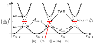
Figure 1: Toroidicity induced SAW continuum gap. The horizontal axis is radial position with $r_{m}$ denoting the $q=m/n$ rational surface, and vertical axis corresponds to $\omega^{2}$. The dashed and solid curves correspond to the SAW continuum in the cylindrical and toroidal limits, respectively; and $\omega_{U}$ and $\omega_{L}$ denote the upper and lower accumulational points of toroidicity induced continuum gap.

3 TAE saturation via nonlinear wave-wave coupling

Nonlinear mode coupling describes the TAE distortion due to interaction with other oscillations, and is expected to play crucial role in TAE nonlinear saturation in future reactors, where system size will be much larger than characteristic orbit size of EPs, and, thus, SAW instabilities with a broad spectrum in toroidal mode numbers will be simultaneously excited by EPs. To illustrate the richness of nonlinear mode couplings of TAE and the strength of gyrokinetic theory in the investigation of underlying physics, three examples are presented, i.e., the nonlinear excitation of $n=0$ zonal field structure (ZFS) by TAE LChenPRL2012 , which corresponds to single-n TAE nonlinear envelope modification via modulational instability; nonlinear spectral evolution of TAE via ion induced scattering TSHahmPRL1995 ; ZQiuNF2019a , which is expected to play crucial role in determining the broad toroidal mode number TAE saturated spectrum and ensuing EP transport; and cross-scale scattering and damping of meso-scale TAE by micro-scale DW LChenNF2022 , suggested by recent experiments as well as simulations showing improved thermal plasma confinement in the presence of significant amount of EPs JCitrinPRL2013 ; ADiSienaNF2019 ; SMazziNP2022 . All these three channels of wave-wave couplings are shown to significantly influence the TAE nonlinear dynamics in different ways, and their relative importance and implications on TAE saturation in burning plasma parameter regimes are discussed. For the sake of simplicity and for consistency with original literature, different notations that are needed are defined only in the corresponding subsection.

3.1 ZFS generation by TAE

Zonal field structures correspond to toroidally and near poloidally symmetric perturbations with $n=0$, and are, thus, linearly stable since they cannot tap the expansion free energy associated with plasma profile nonuniformities. ZFS can be nonlinearly excited by DW turbulence including drift Alfvén waves (DAWs), and in this process, self-consistently scatter DW/DAW into the linearly stable short radial wavelength domain, leading to turbulence regulation and confinement improvement. ZFS excitation was extensively studied in the DWs dynamics ZLinScience1998 ; LChenPoP2000 ; FZoncaPoP2004 ; PDiamondPPCF2005 , observed in simulations with TAEs DSpongPoP1994 ; YTodoNF2010 , while theoretical implications of ZFS to the nonlinear physics of TAE were discussed in LChenPRL2012 . The nonlinear excitation process can be described by the four-wave modulational instability, where upper/lower TAE sidebands due to ZFS modulation are generated, and the nonlinear dispersion relation for ZFS generation can be obtained by the coupled ZFS and TAE sidebands equations. It is noteworthy that, both electrostatic zonal flow (ZF) and electromagnetic zonal magnetic field (zonal current, ZC) should be accounted for on the same footing for the proper understanding of the ZFS generation process FZoncaEPL2015 ; LChenPRL2012 .

For the clarity of presentation, we focus on the modulational instability of TAE originally investigated in Ref. LChenPRL2012 . The further extensions, including the enhanced nonlinear coupling due to existence of “fine-radial-scale" structure ZFS ZQiuNF2017 , and effects of resonant EPs in rendering the ZFS generation process into a forced driven process ZQiuPoP2016 will be only briefly discussed at the end of this section to give the readers a complete picture of the state-of-art research. Considering that TAE constitutes the pump wave $\Omega_{0}(\omega_{0},\mathbf{k}_{0})$ and its upper and lower sidebands $\Omega_{\pm}(\omega_{\pm},\mathbf{k}_{\pm})$ due to the radial modulation of ZFS $\Omega_{Z}(\omega_{Z},\mathbf{k}_{Z})$, and assuming $\Omega_{\pm}=\Omega_{Z}\pm\Omega_{0}$ as the wave vector/frequency matching conditions, the perturbations can be decomposed as

$$\delta\phi_{0} = A_{0}e^{i(n\phi-m_{0}\theta-\omega_{0}t)}\sum_{j}e^{-ij\theta}\Phi_{0}(x-j),$$

$$\delta\phi_{\pm} = A_{\pm}e^{\pm(n\phi-m_{0}\theta-\omega_{0}t)}e^{i(\int k_{Z}dr-\omega_{Z}t)}\sum_{j}e^{\mp ij\theta}\left\{\Phi_{0}(x-j)\atop\Phi^{*}_{0}(x-j)\right\},$$

$$\delta\phi_{Z} = A_{Z}e^{i(\int k_{Z}dr-\omega_{Z}t)}.$$

The frequency and wavenumber matching conditions are already assumed, as illustrated in Fig. 2. We note that, the expression of $\delta\phi_{\pm}$ indicates that the parallel mode structure ($\Phi_{0}$) is not altered by the radial envelope modulation process, which occurs on a longer time scale than the formation of the parallel mode structure itself.

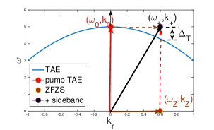
Figure 2: Frequency and wavenumber matching condition for ZFS generation by TAE. Here, the horizontal axis is the radial envelope wavenumber $k_{r}$, and vertical axis is the frequency. The solid curve is the TAE dispersion relation, and $\Delta_{T}$ is the frequency mismatch.

We start from ZFS generation. The first equation for zonal flow generation can be derived from nonlinear vorticity equation. Noting that ZFS have $k_{\parallel Z}=0$, one obtains

$$\frac{n_{0}e^{2}}{T_{i}}\left\langle(1-J^{2}_{Z})\frac{F_{M}}{n_{0}}\right\rangle\delta\phi_{Z}-\sum_{s=e,i}\left\langle\overline{\frac{q}{\omega}J_{Z}\omega_{d}\delta H^{(1)}_{Z}}\right\rangle$$

$$= -\frac{i}{\omega_{Z}}\sum_{\mathbf{k}^{\prime}+\mathbf{k}^{\prime\prime}=\mathbf{k}_{Z}}\Lambda^{k^{\prime}}_{k^{\prime\prime}}\left[\left\langle e(J_{Z}J_{k^{\prime}}-J_{k^{\prime\prime}})\delta L_{k^{\prime}}\delta H_{k^{\prime\prime}}\right\rangle+\frac{c^{2}}{4\pi}k^{\prime\prime 2}_{\perp}\frac{\partial_{l}\delta\psi_{k^{\prime}}\partial_{l}\delta\psi_{k^{\prime\prime}}}{\omega_{k^{\prime}}\omega_{k^{\prime\prime}}}\right].$$

Substituting ion responses of $\Omega_{0}$ and $\Omega_{\pm}$ into RS, noting $k_{\perp}\rho_{i}\lesssim O(1)$, and averaging over fast varying radial scale, one obtains

$$i\omega_{Z}\hat{\chi}_{iZ}\delta\phi_{Z}=-\frac{c}{B_{0}}k_{\theta 0}k_{Z}\left(1-\frac{\omega^{2}_{A}}{4\omega^{2}_{0}}\right)\left(A_{0}A_{-}-A_{0^{*}}A_{+}\right).$$ (26)

Here, $\hat{\chi}_{iZ}\equiv\chi_{iZ}/(k^{2}_{Z}\rho^{2}_{i})$, with $\chi_{iZ}\simeq 1.6k^{2}_{Z}\rho^{2}_{i}q^{2}/\sqrt{\epsilon}$ corresponds to the neoclassical inertial enhancement MRosenbluthPRL1998 , $\omega_{A}=V_{A}/(qR_{0})$ and $1-\omega^{2}_{A}/(4\omega^{2}_{0})\sim O(\epsilon)$ corresponds to the RS and MX non-cancellation due to toroidicity, and finite coupling comes from radial envelope modulation ($\propto k^{2}_{Z}\rho^{2}_{i}$) by ZFS.

The zonal magnetic field equation can be derived from electron parallel force balance equation in stead of the quasi-neutrality condition,

$$\delta E_{\parallel}+\mathbf{b}\cdot\delta\mathbf{u}_{\perp}\times\delta\mathbf{B}_{\perp}/c=0.$$ (27)

Noting that $\delta E_{\parallel}\equiv-\partial_{l}\delta\phi-c\partial_{t}\delta A_{\parallel}$, $\delta\mathbf{u}_{\perp}\simeq c\mathbf{b}\times\nabla_{\perp}\delta\phi/B$, $\delta\mathbf{B}_{\perp}=\nabla\times\delta A_{\parallel}\mathbf{b}$, one also obtains,

$$\delta\psi_{Z}=-\frac{i}{\omega_{0}}\frac{c}{B_{0}}k_{Z}k_{\theta 0}\left(A_{0}A_{-}+A_{0^{*}}A_{+}\right),$$ (28)

where we have introduced the parallel induction potential $\delta\psi_{Z}=\omega_{0}\delta A_{\parallel Z}/(ck_{\parallel 0})$ for ZFS by analogy to the definition of $\delta\psi_{k}$ for TAE. In deriving equation (28), we also noted $\omega_{\pm}=\omega_{Z}\pm\omega_{0}$ as well as ideal MHD condition for TAEs.

The TAE sidebands equations can be derived from nonlinear vorticity equation. We will start with the upper sideband, while the derivation of the governing equations for the lower sideband is similar. Neglecting the curvature coupling term due to the $\lvert\omega\rvert\gg\omega_{G}$ ordering for TAEs, substituting the linear ion responses to $\Omega_{0}$ and $\Omega_{Z}$ into equation (9), and noting $k_{\perp}\rho_{i}\lesssim O(1)$, we have

$$k^{2}_{\perp+}\left[-k^{2}_{\parallel 0}\delta\psi_{+}+\frac{\omega^{2}_{+}}{V^{2}_{A}}\delta\phi_{+}\right]=-i\frac{c}{B_{0}}k_{Z}k_{\theta 0}\left(k^{2}_{Z}-k^{2}_{\perp 0}\right)\frac{\omega_{0}}{V^{2}_{A}}\delta\phi_{0}\left(\delta\phi_{Z}-\delta\psi_{Z}\right).$$ (29)

The other equation for $\Omega_{+}$ can be derived from the electron parallel force balance equation, equation (27), noting that $k_{\parallel 0}=k_{\parallel+}$ and $\delta\phi_{0}\simeq\delta\psi_{0}$ for the pump TAE, and we obtain:

$$\delta\phi_{+}-\delta\psi_{+}=i\frac{c}{B_{0}}k_{Z}k_{\theta 0}\frac{1}{\omega_{0}}\delta\phi_{0}\left(\delta\psi_{Z}-\delta\phi_{Z}\right).$$ (30)

Substituting equation (30) into (29), one then have

$$b_{+}\epsilon_{A+}\delta\phi_{+}=2\frac{i}{\omega_{0}}\frac{c}{B_{0}}k_{\theta 0}k_{Z}b_{0}\delta\phi_{0}\left(\delta\phi_{Z}-\delta\psi_{Z}\right),$$ (31)

with $\epsilon_{A+}$ being the $\Omega_{+}$ dispersion relation in the WKB limit. The $\Omega_{-}$ equation can be derived similarly. Multiplying both sides of equation (31) by $\Phi_{0}$ and averaging over the fast radial scale, one has

$$b_{\pm}\hat{\epsilon}_{A\pm}A_{\pm}=2\frac{i}{\omega_{0}}\frac{c}{B_{0}}k_{\theta 0}k_{Z}b_{0}\left(A_{0}\atop A^{*}_{0}\right)\left(\delta\phi_{Z}-\delta\psi_{Z}\right),$$ (32)

with

$$\hat{\epsilon}_{A\pm} = \left(\omega^{4}_{A}\Lambda_{T}(\omega)D(\omega,k_{Z})/\epsilon_{0}\right)_{\omega=\omega_{\pm}},$$ (33)

$$D(\omega,k_{Z}) = \Lambda_{T}(\omega)-\delta\hat{W}(\omega,k_{Z}),$$ (34)

$\Lambda_{T}\equiv\sqrt{-\Gamma_{l}\Gamma_{u}}$ as given by equation (25), and $\delta\hat{W}(\omega,k_{Z})$ being the normalized potential energy.

The modulational dispersion relation for ZFS generation by TAE can then be derived from equations (26), (28), and (32), and one obtains

$$2\left(\frac{c}{B_{0}}k_{Z}k_{\theta 0}\lvert A_{0}\rvert\right)^{2}\frac{b_{0}}{b_{Z}}\left[\frac{1-\omega^{2}_{A}/(4\omega^{2}_{0})}{\hat{\chi}_{iZ}(\omega_{Z}/\omega_{0})}\left(\frac{1}{\hat{\epsilon}_{A+}}-\frac{1}{\hat{\epsilon}_{A-}}\right)+\left(\frac{1}{\hat{\epsilon}_{A+}}+\frac{1}{\hat{\epsilon}_{A-}}\right)\right]$$

$$=-1,$$ (35)

which can be solved by expanding $D(\omega_{\pm},k_{Z})$ as

$$D(\omega_{\pm},k_{Z})=\pm\frac{\partial D}{\partial\omega_{0}}\left(i\gamma_{Z}\mp\Delta_{T}\right),$$ (36)

with $\gamma_{Z}=-i\omega_{Z}$ and $\Delta_{T}\equiv\omega_{T}(k_{Z})-\omega_{0}$ being the frequency mismatch as shown in Fig. 2, and one obtains

$$\gamma^{2}_{Z} = \left(\frac{c}{B_{0}}k_{Z}k_{\theta 0}\lvert A_{0}\rvert\right)^{2}\frac{b_{0}}{b_{Z}}\frac{\epsilon_{0}}{\Lambda_{T}}\frac{4\omega_{0}/\omega^{2}_{A}}{\partial D_{0}/\partial\omega_{0}}\left[\frac{\Delta_{T}}{\omega_{0}}\frac{\omega^{2}_{0}}{\omega^{2}_{A}}+\frac{1}{\hat{\chi}_{iZ}}\left(\frac{\omega^{2}_{0}}{\omega^{2}_{A}}-\frac{1}{4}\right)\right]-\Delta^{2}_{T},$$

with the first term in the square brackets ($\propto\Delta_{T}/\omega_{0}$) corresponding to the contribution from ZC, while the other term accounts for ZF contribution. It is readily seen that ZF contribution can be of higher order due to the neoclassical shielding ($1/\hat{\chi}_{iZ}\ll 1$) and RS-MX near cancellation by $\omega^{2}_{0}/\omega^{2}_{A}-1/4\sim O(\epsilon)$. Thus, for $\Delta_{T}/\omega_{0}>0$, excitation via the ZC channel can be favoured due to its much lower threshold condition on pump TAE amplitude $A_{0}$. On the other hand, for $\Delta_{T}/\omega_{0}<0$, ZF excitation is still possible, however, on quite stringent conditions; i.e., $\omega^{2}_{0}/\omega^{2}_{A}>1/4$, which corresponds to the pump TAE located in the upper half of the toroidicity induced continuum gap ZQiuEPL2013 and the pump TAE amplitude being large enough to overcome the threshold due to frequency mismatch. It thus suggests that ZFS may be dominated by ZC for $\Delta_{T}/\omega_{0}>0$ due to the trapped-ion enhanced polarizability; thus, a kinetic treatment is necessary. On the other hand, if MHD model without trapped particle effects is adopted, the obtained ZFS excitation condition and corresponding ZFS level will be qualitatively in-correct. This discussion illustrates the richness of the phenomenology underlying the nonlinear route to TAE saturation via wave-wave coupling and ZFS generation. Meanwhile, it also clarifies that the result of numerical simulations may depend on the adopted physics model. Furthermore, it is also worth noting that the “preferential channel via ZC excitation" is connected with the properties of the TAE of interest here, for which RS and MX nearly cancel each other. This argument cannot be straightforwardly generalized to other SAW instabilities; e.g., BAE with $\lvert k_{\parallel}V_{A}/\omega\rvert\ll 1$ will predominantly excite ZF ZQiuNF2016 ; HZhangPST2013 ; while for reversed shear Alfvén eigenmode (RSAE) with frequency between TAE and BAE frequency range, depending on the specific $\lvert nq_{min}-m\rvert$ value, both ZF and/or ZC excitation can be preferred SWeiJPP2021 .

For ZC excitation with $\Delta_{T}/\omega_{0}>0$ and typical parameters of most unstable TAE with $k_{\perp}\rho_{E}\sim O(1)$, the threshold condition can be estimated as

$$\left\lvert\frac{\delta B_{r0}}{B_{0}}\right\rvert^{2}\sim O(10^{-8}\sim 10^{-7}),$$ (38)

which is consistent with the observed magnetic perturbations in present day tokamak experiments WHeidbrinkPRL2007 , suggesting the ZFS excitation can be important for TAE saturation. As the drive by pump TAE is significantly higher than the threshold, the ZFS growth rate is linearly proportional to pump TAE amplitude, typical of spontaneous excitation processes by modulational instability. This feature identifies the parameter space region, where spontaneous excitation is dominant, and clearly distinguishable from, e.g., the forced driven process with the ZFS growth rate determined by the instaneous TAE growth rate, as discussed below ABiancalaniPPCF2021 ; ZQiuPoP2016 .

In the present analysis, only thermal plasma contribution to inertial layer is considered; consistent with EP contribution being negligible in the perpendicular scattering process due to the $k_{\perp}\rho_{E}\gg 1$ ordering. The EP response, however, can play an important role in the ideal region, as addressed in Ref. ZQiuPoP2016 , where it was shown that, as the pump TAE is exponentially growing due to resonant EP contribution, nonlinear EP response to ZFS contributes to the curvature-pressure term in the vorticity equation, dominanting over the RS and MX in the uniform plasma limit. This EP enhanced coupling occurs in the exponentially growing stage of the pump TAE, with ZF excitation dominating over ZC contribution. In that case, the ZF excitation process corresponds to a “forced driven" process, with the ZF growth rate being twice of the instaneous TAE growth rate, as frequently observed in numerical simulations YTodoNF2010 ; ABiancalaniPPCF2021 ; SMazziNP2022 .

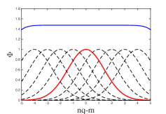
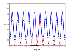
Figure 3: Cartoon for ZFS excitation by strongly ballooning DWs (left panel) v.s. weakly ballooning SAW instabilities (right panel). Here, the dashed curves correspond to the parallel mode structure $\Phi_{0}(nq-m)$ for DWs (left panel) and SAW instabilities (right panel), respectively; while the solid blue curves in both panels correspond to $\sum_{m}\lvert\Phi_{0}\rvert^{2}$. Thus, for DWs with $\sum_{m}\lvert\Phi_{0}\rvert$ being almost independent of $r$ FZoncaPoP2004 , radial envelope modulation leads to meso-scale ZF excitation; while for SAW instabilities, fine-scale structure ZFS is excited.

Another important finding on ZFS excitation by SAW instabilities is due to their weak/moderate ballooning features, corresponding to a smaller or comparable radial width of the parallel mode structure with respect to the distance between mode rational surfaces. As a result, the ZFS excited by TAE has a fine-scale radial structure ZQiuNF2016 ; HZhangPST2013 , in addition to the meso-scale radial envelope corrugation, different from the well-known “meso"-scale ZF excitation in the typically moderately/strongly ballooning DWs, as shown in Fig. 3. This fine-scale radial structure may significantly enhance the ZFS generation rate and its impact on regulating SAW instabilities via the perpendicular scattering. For a comprehensive review of gyrokinetic theory of ZFS generation by TAE, interested readers may refer to Ref. ZQiuNF2017 , where different physics are clarified; e.g., forced driven v.s. spontaneous excitation, meso-scale corrugation v.s. fine-scale structure.

3.2 TAE saturation due to ion induced scattering

Nonlinear ion induced scattering is another potentially important channel for SAW instability nonlinear saturation, corresponding to parametric decay into another SAW and a heavily ion Landau damped ion quasi-mode RSagdeevbook1969 . The role of this process in TAE saturation was originally explored in Ref. TSHahmPRL1995 . It is of particular interest since TAEs lie between two neighbouring mode rational surfaces and are characterized by finite parallel wavenumber $\lvert k_{\parallel}\rvert\simeq 1/(2qR_{0})$, as discussed in Sec. 2.3. Thus, as two counter-propagating TAEs couple, a low frequency mode with finite parallel wavenumber can be generated, i.e., an ion quasi-mode, which can be heavily ion Landau damped, leading to significant consequence on TAE nonlinear dynamics. Compared to ZFS generation investigated in the previous section as a self-interaction process of a single-n TAE, ion induced scattering process is expected to be of particular importance in reactor scale machines with system size being much larger than the characteristic orbit width of fusion alpha particles, where TAEs with multiple toroidal mode numbers and comparable linear growth rates could coexist LChenRMP2016 ; TWangPoP2018 ; ZRenNF2020 . Thus, the ion induced scattering process can determine the saturated spectrum of TAEs and the consequent alpha particle transport rate. Meanwhile, the Landau damping of the nonlinearly generated ion quasi-mode will indirectly transfer the fusion alpha particle power to heat deuterium and tritium ions, providing a potential effective alpha-channeling mechanism TSHahmPST2015 ; NFischNF1994 ; NFischPRL1992 ; ZQiuPRL2018 ; ZQiuNF2019b ; SWeiNF2022 .

The TAE saturation via ion induced scattering was originally investigated in Ref. TSHahmPRL1995 using drift kinetic theory, which was generalized to fusion relevant short wavelength regime with $k^{2}_{\perp}\rho^{2}_{i}\gg\lvert\omega/\Omega_{ci}\rvert$ in Ref. ZQiuNF2019a . Correspondingly, the dominant nonlinear scattering mechanism is qualitatively replaced by the perpendicular scattering LChenEPL2011 , and the saturation level is consequently reduced by one order of magnitude. However, the conceptual workflow of Ref. 38 is similar to that of Ref. TSHahmPRL1995 . In a single scattering process, a pump TAE decays into a counter-propagating sideband TAE and an ion quasi-mode, and the parametric decay process can occur spontaneously as the sideband TAE frequency is lower than that of the pump wave, as shown in Fig. 4.

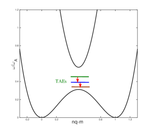
Figure 4: Cartoon of TAE parametric decay in the low-$\beta$ limit.

This process may lead to TAE saturation as the sideband TAE is damped due to the enhanced coupling to lower accumulational point of SAW continuum. As there are many TAEs co-existing, each TAE may simultaneously interact with many TAEs; in some processes it may act as the pump wave, while in some other processes it acts as the decay wave. To analyze this spectral cascading process, the interaction of a representative “test" TAE with a “background" TAE is studied; and the equation for the test TAE nonlinear evolution due to interaction with the background TAE and the ion quasi-mode is derived. In the case of multiple background TAEs simultaneously interacting with the test TAE, one then obtains the equation describing TAE spectral evolution.

Thus, with the linear instability spectrum determined by the equilibrium profiles, the nonlinear process gives the nonlinear saturation spectrum, which eventually determines the electromagnetic fluctuation induced alpha particle transport, as sketched in Fig. 5.

3.2.1 Parametric decay instability

Starting from the nonlinear interaction of the test TAE $\Omega_{0}(\omega_{0},\mathbf{k}_{0})$ with the counter-propagating background TAE $\Omega_{1}(\omega_{1},\mathbf{k}_{1})$, during which the ion sound mode (ISM) $\Omega_{s}(\omega_{s},\mathbf{k}_{s})$ fluctuation is generated, our analysis involves the coupled equations of ISM generation and background TAE evolution. Considering the $\lvert k_{\parallel s}v_{e}\rvert\gg\lvert\omega_{s}\rvert,\lvert\omega_{ds}\rvert$ ordering, and assuming electrostatic ISM, the linear thermal plasma response to ISM can be derived as

$$\delta H^{(1)}_{si} = \frac{e}{T_{i}}F_{M}\frac{\omega_{s}}{\omega_{s}-k_{\parallel s}v_{\parallel}}J_{s}\delta\phi_{s},$$ (39)

$$\delta H^{(1)}_{se} = 0.$$ (40)

Adopting the linear electron response to TAEs derived in equation (10), the nonlinear gyrokinetic equation for electron response to ISW becomes

$$v_{\parallel}\partial_{l}\delta H^{(2)}_{se} = -\sum_{\mathbf{k}^{\prime}+\mathbf{k}^{\prime\prime}=\mathbf{k}}\Lambda^{k^{\prime}}_{k^{\prime\prime}}\delta L_{k^{\prime}}\delta H_{k^{\prime\prime}e}$$ (41)

$$\simeq -\Lambda^{k^{*}_{1}}_{k_{0}}\frac{e}{T_{e}}F_{M}v_{\parallel}\left(\frac{k_{\parallel 1^{*}}}{\omega_{1^{*}}}-\frac{k_{\parallel 0}}{\omega_{0}}\right)\delta\phi_{0}\delta\psi_{1^{*}},$$

with $\Lambda^{k^{*}_{1}}_{k_{0}}\equiv(c/B_{0})\hat{\mathbf{b}}\cdot\mathbf{k_{0}}\times\mathbf{k_{1^{*}}}$. Noting that $\omega_{1^{*}}\simeq-\omega_{0}$, $k_{\parallel 1^{*}}\simeq k_{\parallel 0}$ and consequently that $k_{\parallel s}\simeq 2k_{\parallel 0}$, one has

$$\delta H^{(2)}_{se}\simeq-i\frac{\Lambda^{k^{*}_{1}}_{k_{0}}}{\omega_{0}}\frac{e}{T_{e}}F_{M}\delta\phi_{0}\delta\psi_{1^{*}}.$$ (42)

Nonlinear ion response to $\Omega_{s}$ can be derived noting the $\omega_{s}\sim k_{\parallel s}v_{\parallel}\gg\omega_{ds}$ ordering, and one has

$$\delta H^{(2)}_{si}\simeq-i\frac{\Lambda^{k^{*}_{1}}_{k_{0}}}{\omega_{0}}\frac{e}{T_{i}}F_{M}\frac{k_{\parallel s}v_{\parallel}}{\omega_{s}-k_{\parallel s}v_{\parallel}}J_{0}J_{1}\delta\phi_{0}\delta\phi_{1^{*}}.$$ (43)

It is noteworthy that $\omega_{s}\sim k_{\parallel s}v_{\parallel}$, which is crucial for the resonant wave-particle interactions that determines the scattering process. Substituting equations (41) and (43) into quasi-neutrality condition, one obtains the nonlinear equation for $\Omega_{s}$ generation:

$$\epsilon_{s}\delta\phi_{s}=i\frac{\Lambda^{k^{*}_{1}}_{k_{0}}}{\omega_{0}}\beta_{1}\delta\phi_{0}\delta\phi_{1^{*}},$$ (44)

with $\epsilon_{s}\equiv 1+\tau+\tau\Gamma_{s}\xi_{s}Z(\xi_{s})$ being the ISM linear dispersion relation, $\xi_{s}\equiv\omega_{s}/(k_{\parallel s}v_{it})$, $Z(\xi_{s})$ being the well-known plasma dispersion function defined as

$$Z(\xi_{s})\equiv\frac{1}{\sqrt{\pi}}\int^{\infty}_{-\infty}\frac{e^{-y^{2}}}{(y-\xi_{s})}dy,$$

the nonlinear coupling coefficient $\beta_{1}=1+\tau F_{1}(1+\xi_{s}Z(\xi_{s}))$ and $F_{1}\equiv\langle J_{0}J_{1}J_{s}F_{M}/n_{0}\rangle$.

The nonlinear particle response to the test TAE, can be derived as

$$\delta H^{(2)}_{0e} = -\frac{(\Lambda^{k^{*}_{1}}_{k_{0}})^{2}}{\omega^{2}_{0}}\frac{e}{T_{e}}F_{M}\lvert\delta\phi_{1}\rvert^{2}\delta\phi_{0},$$ (45)

$$\delta H^{(2)}_{0i} = i\frac{\Lambda^{k^{*}_{1}}_{k_{0}}}{\omega_{0}}\frac{e}{T_{i}}F_{M}\frac{k_{\parallel s}v_{\parallel}}{\omega_{s}-k_{\parallel s}v_{\parallel}}\left[J_{1}J_{s}\delta\phi_{s}\delta\phi_{1}-i\frac{\Lambda^{k^{*}_{1}}_{k_{0}}}{\omega_{0}}J^{2}_{1}J_{0}\lvert\delta\phi_{1}\rvert^{2}\delta\phi_{0}\right].$$ (46)

In deriving $\delta H^{(2)}_{0e}$ and $\delta H^{(2)}_{0i}$, the nonlinear particle responses to $\Omega_{s}$ are also included due to the fact that it may be heavily ion Landau damped. One then obtains,

$$\delta\psi_{0}=\left(1+\sigma^{(2)}_{0}\right)\delta\phi_{0}+D_{0}\delta\phi_{1}\delta\phi_{s},$$ (47)

with $\sigma^{(2)}_{0}\equiv(\Lambda^{k^{*}_{1}}_{k_{0}})^{2}\left[-1+\tau F_{2}(1+\xi_{s}Z(\xi_{s})\right]\lvert\delta\phi_{1}\rvert^{2}/\omega^{2}_{0}$, $D_{0}=i\tau\Lambda^{k^{*}_{1}}_{k_{0}}F_{1}[1+\xi_{s}Z(\xi_{s})]/\omega_{0}$, and $F_{2}=\langle J^{2}_{0}J^{2}_{1}F_{M}/n_{0}\rangle$.

The other equation of $\Omega_{0}$ can be derived from nonlinear vorticity equation as

$$b_{0}\left[\frac{1-\Gamma_{0}+\alpha^{(2)}_{0}/\omega^{2}_{0}}{b_{0}}\delta\phi_{0}-\frac{k^{2}_{\parallel 0}V^{2}_{A}}{\omega^{2}_{0}}\delta\psi_{0}\right]=D_{2}\delta\phi_{1}\delta\phi_{s},$$ (48)

with

$$\alpha^{(2)}_{0} = (\Lambda^{k^{*}_{1}}_{k_{0}})^{2}(F_{2}-F_{1})(1+\xi_{s}Z(\xi_{s}))\lvert\delta\phi_{1}\rvert^{2},$$

$$D_{2} = -i\Lambda^{k^{*}_{1}}_{k_{0}}[F_{1}(1+\xi_{s}Z(\xi_{s}))-\Gamma_{s}\xi_{s}Z(\xi_{s})-\Gamma_{1}]/\omega_{0}.$$

From equations (47), (48) and (44), one obtains the following nonlinear eigenmode equation of the test TAE $\Omega_{0}$ due to interaction with the background TAE $\Omega_{1}$

$$b_{0}\left(\epsilon_{A0}+\epsilon^{(2)}_{0}\right)\delta\phi_{0}=-\frac{(\Lambda^{k^{*}_{1}}_{k_{0}})^{2}\beta_{1}\beta_{2}}{\tau\epsilon_{s}}\lvert\delta\phi_{1}\rvert^{2}\delta\phi_{0},$$ (49)

with $\beta_{2}\equiv\beta_{1}-\epsilon_{s}$. Multiplying both sides of equation (49) with $\Phi^{*}_{0}$, and averaging over the fast radial scale of $1/(n_{s}q^{\prime})\ll\delta\ll 1/(n_{0}q^{\prime})$, one then obtains

$$\left(\hat{\epsilon}_{A0}-\Delta_{0}\lvert A_{1}\rvert^{2}-\chi_{0}\epsilon_{s}\lvert A_{1}\rvert^{2}\right)A_{0}=-(\hat{C}_{0}/\epsilon_{s})\lvert A_{1}\rvert^{2}A_{0},$$ (50)

with $\hat{\epsilon}_{A0}$ being the $\Omega_{0}$ linear eigenmode dispersion relation obtained from $\hat{\epsilon}_{A0}\equiv\int\lvert\Phi_{0}\rvert^{2}\epsilon_{A0}dr/\int\lvert\Phi_{0}\rvert^{2}dr$, $\Delta_{0}$, $\chi_{0}$ and $\hat{C}_{0}$ corresponding, respectively, to nonlinear frequency shift, ion Compton scattering and shielded-ion scattering. Their specific expressions can be found in Ref. ZQiuNF2019a . Equation (50) can be understood as the parametric dispersion relation for $\delta\phi_{1}$ decaying into $\delta\phi_{0}$ and $\delta\phi_{s}$ and the condition for the nonlinear process to occur can be determined for different parameter regimes that crucially enter through the properties of $\delta\phi_{s}$.

For typical tokamak parameters with $\tau\sim O(1)$, $\Omega_{s}$ is heavily Landau damped with $\lvert\epsilon_{s,I}\rvert$ comparable to $\lvert\epsilon_{s,R}\rvert$, with subscripts “$R$" and “$I$" denoting real and imaginary parts. One then has, from the imaginary part of equation (50),

$$\gamma+\gamma_{0}=\frac{\lvert A_{1}\rvert^{2}}{\partial_{\omega_{0}}\epsilon_{0,R}}\left(\frac{\hat{C}_{0}}{\lvert\epsilon_{s}\rvert^{2}}+\chi_{0}\right)\epsilon_{s,I}.$$ (51)

with $\hat{C}_{0}$ and $\chi_{0}$ corresponding, respectively, to the shielded-ion and nonlinear ion Compton scatterings. Since both $\hat{C}_{0}$ and $\chi_{0}$ are positive definite, and that $\epsilon_{s,I}=\sqrt{\pi}\tau\Gamma_{s}\xi_{s}\exp(-\xi^{2}_{s})$ with $\xi_{s}\equiv(\omega_{0}-\omega_{1})/\lvert k_{\parallel s}v_{it}\rvert$, one then has, $\gamma>0$ corresponds to $\omega_{1}>\omega_{0}$, i.e., the parametric decay spontaneously occur as the pump TAE frequency is higher than the sideband TAE. Thus, the above discussed parametric decay process will lead to power transfer from higher frequency part of the spectrum to the lower frequency part RSagdeevbook1969 ; TSHahmPRL1995 , as shown in Fig. 5. The sideband TAE, with lower frequency, can be saturated due to enhanced damping due to coupling to the lower part of the SAW continuum.

3.2.2 Spectral evolution

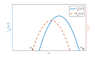
Figure 5: Cartoon of TAE spectral cascading due to ion induced scattering. The horizontal axis is the mode frequency, solid curve is the linear growth rate while the dashed curve is the saturated spectrum due to ion induced scattering.

The spontaneous power transfer from $\delta\phi_{1}$ to $\delta\phi_{0}$ investigated above can lead to TAE scattering to the lower frequency fluctuation spectrum. In burning tokamak plasma of reactor scale, where multiple TAEs coexist, characterized by comparable frequencies and growth rates, each TAE can interact with the “bath" of background TAEs, and this process can be described by an equation for spectral evolution derived from equation (50). Denoting the generic test TAE with subscript $k$ and background TAE with subscript $k_{1}$, and summing over all background TAEs, one obtains

$$\hat{\epsilon}_{Ak}A_{k}=\sum_{k_{1}}\left(\Delta_{0}+\chi_{0}\epsilon_{s}-\frac{\hat{C}_{0}}{\epsilon_{s}}\right)\lvert A_{k_{1}}\rvert^{2}A_{k}.$$ (52)

Multiplying equation (52) with $A^{*}_{k}$, and taking the imaginary part, we then obtain the equation describing TAE nonlinear evolution due to interaction with the bath of TAEs:

$$\left(\partial_{t}-2\gamma_{L}(k)\right)I_{k}=\frac{2}{\partial_{\omega_{k}}\hat{\epsilon}_{Ak,R}}\sum_{k_{1}}\frac{1}{k^{2}_{\perp 1}}\left(\frac{\hat{C}_{0}}{\lvert\epsilon_{s}\rvert^{2}}+\chi_{0}\right)\epsilon_{s,i}I_{k_{1}}I_{k},$$ (53)

which can be rewritten as

$$\left(\partial_{t}-2\gamma_{L}(\omega)\right)I_{\omega}=\frac{2}{\partial_{\omega}\epsilon_{\omega,R}}\int^{\omega_{M}}_{\omega_{L}}d\omega^{\prime}V(\omega,\omega^{\prime})I_{\omega^{\prime}}I_{\omega},$$ (54)

with $I_{\omega}=\sum_{k}I_{k}\delta(\omega-\omega_{k})$ being the continuum version of $I_{k}$, $I_{k}\equiv\lvert\nabla_{\perp}A_{k}\rvert^{2}$, $\omega_{M}$ being the highest frequency for TAE to be linearly unstable, and $\omega_{L}$ being the lowest frequency of TAE spectrum, which is, in fact, linearly stable, and nonlinearly excited in the downward cascading process, as shown by Fig. 5. The integration kernel $V(\omega,\omega^{\prime})$ is given by

$$V(\omega,\omega^{\prime})\equiv\frac{1}{k^{2}_{\perp\omega^{\prime}}}\left(\frac{\hat{C}_{0}}{\lvert\epsilon_{s}\rvert^{2}}+\chi_{0}\right)\epsilon_{s,i}.$$ (55)

The saturated TAE spectrum can thus be derived from the fixed point solution of equation (54) by taking $\partial_{t}I_{\omega}=0$. The obtained integral equation, can be reduced to a differential equation noting that $I_{\omega^{\prime}}$ varies in $\omega^{\prime}$ much slower than $V(\omega,\omega^{\prime})$, with the former varying on the scale of $\lvert\omega_{M}-\omega_{L}\rvert\simeq\epsilon_{0}\omega_{A}$, while the latter on the scale of $\lvert v_{it}/(qR_{0})\rvert$ determined by $\epsilon_{s,I}$. Thus, noting $I_{\omega^{\prime}}=I_{\omega}-\omega_{s}\partial_{\omega}I_{\omega}$, and $\lvert\omega_{M}-\omega_{L}\rvert\sim\epsilon_{0}\omega_{A}\gg\omega_{s}$ for the ion induced scattering process to be important as shown in Fig. 4, one has

$$\gamma_{L}(\omega) = -\frac{1}{\partial_{\omega}\epsilon_{\omega,R}}\int^{\omega-\omega_{L}}_{\omega-\omega_{M}}d\omega_{s}V(\omega_{s})\left(I_{\omega}-\omega_{s}\partial_{\omega}I_{\omega}\right)$$ (56)

$$= -\frac{1}{\partial_{\omega}\epsilon_{\omega,R}}\left[U_{0}I_{\omega}-U_{1}\partial_{\omega}I_{\omega}\right].$$

with

$$U_{0} \equiv \int^{\omega-\omega_{L}}_{\omega-\omega_{M}}d\omega_{s}V(\omega_{s})\simeq\int^{\infty}_{-\infty}d\omega_{s}V(\omega_{s})\rightarrow 0,$$ (57)

$$U_{1} \equiv \int^{\omega-\omega_{L}}_{\omega-\omega_{M}}d\omega_{s}\omega_{s}V(\omega_{s})\simeq\int^{\infty}_{-\infty}d\omega_{s}\omega_{s}V(\omega_{s})$$ (58)

$$\simeq \frac{\pi^{3/2}}{2k^{2}_{\perp}}\left(\frac{\hat{C}_{0}}{\lvert\epsilon_{s}\rvert^{2}}+\chi_{0}\right)k^{2}_{\parallel s}v^{2}_{it}.$$

In deriving equations (57) and (58), it is noted that $V(\omega_{s})\propto\epsilon_{s,I}$ is odd function of $\omega_{s}$. Equation (56) is the desired differential equation for the saturated spectrum, and gives

$$I_{\omega}=\frac{2k_{\parallel s}v_{it}\omega_{M}\gamma_{L}(\omega_{M})}{U_{1}}-\frac{1}{U_{1}}\int^{\omega_{M}}_{\omega}\gamma_{L}\partial_{\omega}\epsilon_{\omega,R}d\omega,$$ (59)

which, after integrating over the fluctuation population zone, yields the overall TAE intensity

$$I_{Sat}\equiv\int^{\omega_{M}}_{\omega_{L}}I_{\omega}d\omega\simeq\frac{\overline{\gamma_{L}}}{U_{1}}\omega^{3}_{T}\epsilon^{2}_{eff},$$ (60)

with $\epsilon_{eff}\equiv 1-\omega_{M}/\omega_{L}\sim O(\epsilon)$. Noting that $\lvert\delta B_{r}\rvert^{2}\simeq\lvert k_{\theta}\delta A_{\parallel}\rvert^{2}=\lvert ck_{\theta}k_{\parallel}/(\omega k_{r})\rvert^{2}I_{Sat}$, one then obtains the saturation level of the magnetic fluctuations

$$\lvert\delta B_{r}\rvert^{2}\simeq\frac{c^{2}\epsilon^{2}\epsilon^{2}_{eff}}{2\pi^{3/2}}\frac{\omega_{T}\overline{\gamma_{L}}k^{2}_{r}}{(\hat{C}_{0}/\lvert\epsilon_{s}\rvert^{2}+\chi_{0})\Omega^{2}_{ci}\rho^{2}_{it}},$$ (61)

which then yields, for typical parameters in burning plasma regime, the scaling law for the magnetic perturbations,

$$\left\lvert\frac{\delta B_{r}}{B_{0}}\right\rvert^{2} \sim \frac{m_{i}}{8\tau\pi^{3/2}e^{2}\mu_{0}}\frac{\overline{\gamma_{L}}}{\omega_{T}}\frac{T^{2}_{E}}{T^{2}_{i}}q^{2}n^{-1}_{0}\epsilon^{6}R^{-2}_{0}$$ (62)

$$\sim 1.2\times 10^{15}A_{m}q^{2}n^{-1}_{0}\epsilon^{6}R^{-2}_{0}\frac{T^{2}_{E}}{T^{2}_{i}}\frac{\overline{\gamma_{L}}}{\omega_{T}}.$$

Here, $A_{m}$ is the mass ratio of thermal ion to proton, and $n_{0}$ is the thermal plasma density. For typical parameters of reactors, e.g., ITER KTomabechiNF1991 or CFETR YWanNF2017 , the expected magnetic fluctuation level is $\lvert\delta B_{r}/B_{0}\rvert^{2}\sim O(10^{-8}\sim 10^{-7})$. It is noteworthy that the obtained TAE magnetic perturbation depends sensitively on the local inverse aspect ratio $\epsilon$, which is, however, not surprising, since TAE exist due to toroidicity ($\propto\epsilon$) induced SAW continuum gap and the saturation process, determined by ion-induced scattering, is the TAE downward spectrum cascading (by $\sim\epsilon\omega_{A}$) that leads to enhanced coupling to SAW continuum.

3.2.3 EP transport

The TAE induced fusion alpha particle transport, can be obtained from nonlinear gyrokinetic transport theory LChenJGR1999 ; LChenRMPP2021 , with the expected magnetic fluctuation level given by equation (62). Here, taking circulating EP as an example, whose transport is mainly caused by resonance overlapping induced EP orbit stochasticity TWangPoP2019 , the quasilinear transport equation for EP equilibrium distribution function evolution is LChenJGR1999 ; ABrizardPoP1995

$$\partial_{t}F_{0E}=-\overline{\sum_{\mathbf{k}=\mathbf{k^{\prime}}+\mathbf{k^{\prime\prime}}}\Lambda^{k^{\prime}}_{k^{\prime\prime}}J_{k^{\prime}}\delta L_{k^{\prime}}\delta H_{k^{\prime\prime}}},$$ (63)

with $\mathbf{k}=k_{Z}\hat{\mathbf{r}}=\mathbf{k^{\prime}}+\mathbf{k^{\prime\prime}}$ denoting the bounce averaged phase space zonal structure modulation MFalessiPoP2019 in the radial direction. Meanwhile, the perturbed linear EP distribution function for well circulating EPs can be given by ZQiuPoP2016 ; GFuPoFB1992

$$\delta H_{kE}=-\frac{e}{m}Q_{k}F_{0E}J_{k}\delta L_{k}\sum_{l,p}\frac{J_{l}(\hat{\lambda}_{k})J_{p}(\hat{\lambda}_{k})e^{-i(l-p)(\theta-\theta_{0r})}}{\omega_{k}-k_{\parallel}v_{\parallel}+l\omega_{tr}},$$ (64)

with $QF_{0E}\equiv(\omega\partial_{E}-\hat{\omega}_{*})F_{0E}$, $F_{0E}$ being equilibrium EP distribution function, $\hat{\lambda}_{k}=k_{\perp}\hat{v}_{d}/\omega_{tr}$ denoting finite drift orbit width effects, and $\theta_{0r}\equiv\tan^{-1}(k_{r}/k_{\theta})$. Substituting equation (64) into equation (63) and integrating over velocity space, one then obtains,

$$\partial_{t}n_{0E}\simeq-\partial_{r}\left(D_{Res}\partial_{r}n_{0E}\right),$$ (65)

with $n_{0E}$ being the equilibrium EP density, the resonant circulating EP radial diffusion rate given as

$$D_{Res}\equiv\left\langle 2\pi\sum_{l}\lvert\delta V_{Er,l}\rvert^{2}J^{2}_{l}(\hat{\lambda}_{l})\delta(\omega-k_{\parallel}v_{\parallel}+l\omega_{tr})\frac{F_{0E}}{n_{0E}}\right\rangle,$$ (66)

and $\lvert\delta V_{Er,l}\rvert\equiv ck_{\theta}J_{k}\lvert\delta\phi_{k}\rvert l\omega_{tr}/(B_{0}\omega_{k})$ being the resonant EP electric-field drift velocity. Substituting the saturated TAE fluctuation given by equation (61) into equation (66), and noting again $\lvert\delta\phi\rvert^{2}=\omega^{2}\delta B^{2}_{r}/(c^{2}k^{2}_{\theta}k^{2}_{\parallel})$, one obtains,

$$D_{Res}\simeq\frac{1}{4}\frac{V_{A}}{k_{\parallel 0}}\left\lvert\frac{\delta B_{r}}{B_{0}}\right\rvert^{2},$$ (67)

corresponding to the resonant EP transit time $\omega^{-1}_{tr,Res}$ being the wave-particle de-correlation time. The scaling law for TAE induced circulating EP diffusion rate can then be derived as

$$D_{Res}\sim 1.3\times 10^{31}A^{1/2}_{m}\epsilon^{6}q^{3}n^{-3/2}_{0}R^{-1}_{0}\frac{T^{2}_{E}}{T^{2}_{i}}\frac{\overline{\gamma_{L}}}{\omega_{T}}.$$ (68)

For typical parameters of a reactor-size tokamak, the TAE induced resonant circulating EP diffusion rate can be estimated as $D_{Res}\sim 1-10\ m^{2}/s$ for $\epsilon\sim 1/6-1/3$.

3.2.4 Open questions

The present analysis of TAE saturation via nonlinear ion-induced scattering extends the previous work based on drift kinetic theory TSHahmPRL1995 , and gaves a more quantitatively accurate estimation of the TAE saturation level and, thus, of the fusion alpha particle transport rate. For a predictive ability of the impact on fusion plasma performance, besides validation of the present analytical results using first-principle-based large scale simulations, there are several factors, which remain to be explored.

First, the present analysis neglects the nonuniformity of bulk plasma, and focuses on the scattering off ion quasi mode. However, in the nonlinear parametric decay of kinetic Alfvén wave (KAW), it has been demonstrated that bulk plasma nonuniformity may significantly affect the nonlinear process, by enhancing the ion Compton scattering rate by an order of magnitude since $\lvert\omega_{*i}\rvert\gg\lvert k_{\parallel s}v_{it}\rvert$. Furthermore, plasma nonuniformity qualitatively breaks the parity of the decay KAW spectrum and may have significant implications on finite momentum transport LChenPoP2022 . As the TAE cascading process of interest in the present review has a one-to-one correspondence to the KAW parametric decay in slab geometry, we expect that thermal plasma nonuniformity may also have an important consequence on the TAE saturation; this aspect will be further explored in a separate work ZChengNF2023 .

Second, the nonlinearly generated ion quasi-mode in the present analysis, or drift sound wave as bulk plasma nonuniformity is accounted for, are both heavily ion Landau damped,. Thus, they provide a channel for nonlinearly transfer the alpha particle power to fuel deuterium-tritium ions, as originally proposed and investigated in Ref. TSHahmPST2015 based on the results from Ref. TSHahmPRL1995 . Deriving the ion heating power from the present results and evaluating the implications to sustained burning may provide elements of crucial importance for reactors with high temperature plasma and thus low collisonality.

The third point to be explored is alpha particle global transport and the steady state alpha particle as well as bulk plasma profiles in reactor relevant conditions. In fact, equation (68) provides an estimate of local transport. However, the feedbacks of alpha particle driven instabilities on bulk plasmas and energetic particles themselves via different channels ADiSienaNF2019 ; JCitrinPRL2013 ; LChenNF2023 should be properly taken into account.

3.3 TAE scattering and damping by DW turbulence

The last nonlinear process to be discussed is TAE scattering by DW turbulence. Microscopic DW turbulence driven by expansion free energy associated with plasma nonuniformities is another significant low frequency fluctuation in magnetically confined plasmas, and is crucial for thermal plasma transport WHortonRMP1999 . DWs typically have frequencies comparable to plasma diamagnetic frequency, and perpendicular wavelength in the range of thermal ion Larmor radius or even shorter, when electron dynamics plays an important role. With different free energy sources, DWs may be driven as ion temperature gradient mode, trapped electron modes, etc., and be predominant in different frequency range of the spectrum. Effects of DWs on EP transport were investigated in Refs. WZhangPRL2008 ; ZFengPoP2013 , suggesting that the direct EP transport by DWs can be negligible due to the scale separation between EP orbit size and typical DW perpendicular wavelength. This result is consistent with theoretical expectations and should be considered a well assessed fact, despite some discussions of about a decade ago, due to the anomaly in EP confinement that was reported by AUG SGunterNF2007 , JT-60U TSuzukiNF2008 and DIII-D WHeidbrinkPRL2009 . In fact, it was demonstrated that the observed behavior was due to ITG driven diffusion of EP with low relative energy $E$ w.r.t. the core thermal energy $T_{c}$. For $E/T_{c}\gtrsim 10$, the EP diffusivity is typically an order of magnitude less than that of core plasma ions SZwebenNF2000 , and, thus, “EP transport by microturbulence in reactor relevant conditions and above the critical energy (at which plasma ions and electrons are heated at equal rates by EPs) is negligible and EP turbulent diffusivities have intrinsic interest mostly in present day experiments with low characteristic values of $E/Tc$." LChenRMP2016 . On the other hand, EP may influence the DWs stability via many mechanisms, such as thermal ion dilution GTardiniNF2007 , modification of curvature by increased pressure gradient CBourdelleNF2005 , etc. For the reference of EP stabilization of DW turbulence, interested readers may refer to a recent review by Citrin et al JCitrinPPCF2023 .

With two fundamental fluctuations groups coexisting, DWs and SAWs, or more precisely drift Alfvén waves (DAWs), characterized by distinct spatial and temporal scales, and dominating transport in different energy ranges, it is natural to consider their mutual effects. The nonlinear interactions of DWs and SAW instabilities via ZFS have been proposed theoretically LChenRMP2016 ; LChenPRL2012 ; ZQiuPoP2016 ; LChenNF2001 ; ZQiuNF2016 ; FZoncaPPCF2015 and investigated numerically YTodoNF2010 ; DSpongPoP1994 ; HZhangPST2013 , and were suggested as possible interpretation of experimental observation of confinement improvement with large fraction of EPs JCitrinPRL2013 ; ADiSienaNF2019 ; ADiSienaJPP2021 ; SMazziNP2022 . This “indirect channel" remains to be investigated in more detail due to the multiple facets consiting of complex nonlinear behaviours. It was proposed, in our recent work, that the DWs and SAW instabilities can also mutually interact via direct nonlinear mode coupling processes, which can lead to, e.g., suppression of TAE due to the scattering by finite amplitude electron DW (eDW) LChenNF2022 . The “inverse" process, on the other hand, shows that finite amplitude TAE has negligible effects on the eDW stability LChenNF2023 . This paradigm, proposed using TAE and eDW as example, can be generalized to include other effects such as trapped electron contribution. Here, we will briefly review the TAE scattering by finite amplitude eDW.

The TAE-eDW scattering process, can be understood as the test TAE “linear" stability in the presence of finite amplitude eDW, and can be considered as a two-step process. In the first process, short wavelength upper and lower kinetic Alfvén wave (KAW) sidebands are generated, with frequency comparable to TAE and high toroidal mode number determined by eDW. In the second step, KAW then couple with eDW and feed back on the test TAE, modifying its dispersive properties and stability as shown in Fig. 6. The damping of the mode-converted upper and lower KAWs, as shown in Fig. 7, then lead to the damping of the test TAE.

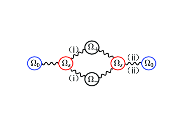
Figure 6: Cartoon of the two-step nonlinear process of TAE scattering by eDW. The first process corresponds to short scale KAW sidebands generation due to eDW scattering, while the second corresponds to their feedback on the test TAE.

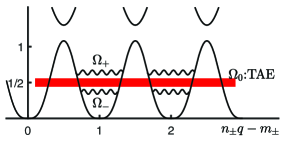
Figure 7: Cartoon of upper and lower KAWs generation due to TAE-eDW scattering, and coupling to continuum.

3.3.1 KAW generation

We start from the upper sideband $\Omega_{+}$ generation channel due to test TAE $\Omega_{0}$ and eDW $\Omega_{s}$ coupling, noting that the analysis for $\Omega_{-}$ is similar. The linear and nonlinear particle responses to $\Omega_{+}$, can be derived noting the $\lvert k_{\parallel}v_{te}\rvert\gg\lvert\omega_{+}\rvert\gg\lvert k_{\parallel}v_{ti}\rvert$ ordering, and one has, to the leading order,

$$\delta H^{(1)}_{+i} \simeq \frac{e}{T_{i}}F_{M}\left(1-\frac{\omega_{*i}}{\omega}\right)_{+}J_{+}\delta\phi_{+},$$ (69)

$$\delta H^{(1)}_{+e} \simeq -\frac{e}{T_{e}}F_{M}\left(1-\frac{\omega_{*e}}{\omega}\right)_{+}\delta\psi_{+}.$$ (70)

The nonlinear ion response to $\Omega_{+}$ can be derived as

$$\delta H^{(2)}_{+,i}\simeq-i\frac{\Lambda^{s}_{0}}{2\omega_{0}}J_{0}J_{s}\frac{e}{T_{i}}F_{M}\left(\frac{\omega_{*i}}{\omega}\right)_{s}\delta\phi_{s}\delta\phi_{0},$$ (71)

having noted the linear ion response to $\Omega_{0}$ and $\Omega_{s}$. On the other hand, nonlinear electron contribution to upper KAW can be neglected, since $\Omega_{s}$ is predominantly electrostatic. Substituting the particle responses into quasi-neutrality condition, we then have,

$$\delta\psi_{+}=\sigma_{*+}\delta\phi_{+}+i\frac{\Lambda^{s}_{0}}{2\omega_{0}}D_{+}\delta\phi_{0}\delta\phi_{s},$$ (72)

where $\sigma_{*k}$, derived in equation (13), denotes the deviation from ideal MHD condition due to plasma nonuniformity and/or FLR effects, while $D_{+}=\tau(\omega_{*i}/\omega)_{s}F_{+}/(1-\omega_{*e}/\omega)_{+}$ denotes nonlinear contribution with $F_{+}=\langle J_{0}J_{s}J_{+}F_{M}/n_{0}\rangle_{v}$. The other equation for $\Omega_{+}$, can be derived from nonlinear vorticity equation, by substituting the linear particle responses to $\Omega_{0}$ and $\Omega_{s}$ into the Reynolds stress term

$$\tau b_{+}\left[\left(1-\frac{\omega_{*i}}{\omega}\right)_{+}\frac{(1-\Gamma_{+})}{b_{+}}\delta\phi_{+}-\left(\frac{V^{2}_{A}}{b}\frac{k_{\parallel}bk_{\parallel}}{\omega^{2}}\right)_{+}\delta\psi_{+}\right]$$ (73)

$$= -i\frac{\Lambda^{s}_{0}}{2\omega_{0}}\gamma_{+}\delta\phi_{0}\delta\phi_{s},$$

with $\gamma_{+}=\tau[\Gamma_{s}-\Gamma_{0}+(\omega_{*i}/\omega)_{s}(F_{+}-\Gamma_{s})]$.

Combining equations (72) and (73), one obtains, the equation for upper KAW generation due to $\Omega_{0}$ and $\Omega_{s}$ coupling

$$\tau b_{+}\epsilon_{A+}\delta\phi_{+}=-i(\Lambda^{s}_{0}/2\omega_{0})\beta_{+}\delta\phi_{s}\delta\phi_{0},$$ (74)

where $\epsilon_{A+}$ is the linear SAW/KAW operator given by equation (16) with curvature coupling term neglected due to high TAE frequency range, and

$$\beta_{+} = \tau(\Gamma_{s}-\Gamma_{0})+\tau\left(\frac{\omega_{*i}}{\omega}\right)_{s}\left[F_{+}-\Gamma_{s}-\left(\frac{k_{\parallel}bk_{\parallel}}{\omega^{2}}\right)_{+}\frac{\tau V^{2}_{A}F_{+}}{(1-\omega_{*e}/\omega)_{+}}\right].$$ (75)

The generation of lower KAW $\Omega_{-}$ due to $\Omega^{*}_{0}$ and $\Omega_{s}$ coupling, can be derived similarly as

$$\tau b_{-}\epsilon_{A-}\delta\phi_{-}=i(\Lambda^{s}_{0}/2\omega_{-})\beta_{-}\delta\phi_{s}\delta\phi^{*}_{0},$$ (76)

with

$$\beta_{-}=\tau(\Gamma_{s}-\Gamma_{0})+\tau\left(\frac{\omega_{*i}}{\omega}\right)_{s}\left[F_{-}-\Gamma_{s}-\left(\frac{k_{\parallel}bk_{\parallel}}{\omega^{2}}\right)_{-}\frac{\tau V^{2}_{A}F_{-}}{(1-\omega_{*e}/\omega)_{-}}\right].$$ (77)

3.3.2 Feedback to $\Omega_{0}$ and consequence on TAE stability

The effect of eDW scattering on the test TAE, can be derived by accounting for feedback of $\Omega_{\pm}$ via nonlinear coupling to $\Omega_{s}$. Here, we only discuss the contribution to $\Omega_{0}$ by nonlinear coupling between $\Omega_{+}$ and $\Omega^{*}_{s}$, noting that the contribution due to $\Omega_{-}$ and $\Omega_{s}$ coupling can be derived similarly.

The nonlinear ion response to $\Omega_{0}$ can be derived as

$$\delta H^{(2)}_{0i} \simeq \frac{e}{T_{i}}F_{M}\left(\frac{\omega_{*i}}{\omega}\right)_{s}\left[i\frac{\Lambda^{s}_{0}}{2\omega_{0}}J_{s}J_{+}\delta\phi^{*}_{s}\delta\phi_{+}+\left(\frac{\Lambda^{s}_{0}}{2\omega_{0}}\right)^{2}J_{0}J^{2}_{s}\lvert\delta\phi_{s}\rvert^{2}\delta\phi_{0}\right]$$ (78)

$$+ \delta\phi_{-}\ \mbox{contribution},$$

with the second term corresponding to $\delta H^{(2)}_{+i}$ contribution. The nonlinear electron response to $\Omega_{0}$ is negligible. The quasi-neutrality condition then yields

$$\delta\psi_{0}=\left(\sigma_{*0}+\alpha_{0}\lvert\delta\phi_{s}\rvert^{2}\right)\delta\phi_{0}-i(\Lambda^{s}_{0}/2\omega_{0})D^{+}_{0}\delta\phi^{*}_{s}\delta\phi_{+}+\delta\phi_{-}\ \mbox{contribution},$$ (79)

with $\alpha_{0}=-(\Lambda^{s}_{0}/2\omega_{0})^{2}\tau(\omega_{*i}/\omega)_{s}F_{2}$, $F_{2}\equiv\langle J^{2}_{0}J^{2}_{s}F_{M}/n_{0}\rangle_{v}$ mainly contributing to nonlinear frequency shift, while $D^{+}_{0}=\tau(\omega_{*i}/\omega)_{s}F_{+}/(1-\omega_{*e}/\omega)_{0}$.

The other equation for $\Omega_{0}$ can then be derived from nonlinear vorticity equation, as

$$\tau b_{0}\left\{\left[\left(1-\frac{\omega_{*i}}{\omega_{0}}\right)_{0}\frac{(1-\Gamma_{0})}{b_{0}}+\alpha^{+}_{0}\lvert\delta\phi_{s}\rvert^{2}\right]\delta\phi_{0}-\left(\frac{V^{2}_{A}}{b}\frac{k_{\parallel}bk_{\parallel}}{\omega^{2}}\right)_{0}\delta\psi_{0}\right\}$$ (80)

$$= i\frac{\Lambda^{s}_{0}}{2\omega_{0}}\gamma^{+}_{0}\delta\psi^{*}_{s}\delta\phi_{+}+\delta\phi_{-}\ \mbox{contribution}.$$

Substituting equation (79) into (80), and neglecting the nonlinear frequency shift while focusing on the stability of the test TAE due to scattering by background eDW, one then obtains

$$\tau b_{0}\epsilon_{A0}\delta\phi_{0}=i\frac{\Lambda^{s}_{0}}{2\omega_{0}}\beta^{+}_{0}\delta\phi^{*}_{s}\delta\phi_{+}+\delta\phi_{-}\ \mbox{contribution}.$$ (81)

Substituting $\delta\phi_{+}$ from equation (74) into (81), one obtains,

$$\tau b_{0}\epsilon_{A0}\delta\phi_{0}=\left[\left(\frac{\Lambda^{s}_{0}}{2\omega_{0}}\right)^{2}\beta^{+}_{0}\delta\phi^{*}_{s}\frac{\beta_{+}}{\tau b_{+}\epsilon_{A+}}\delta\phi_{s}\right]\delta\phi_{0}+\delta\phi_{-}\ \mbox{contribution},$$ (82)

which can be solved noting the spatial scale separation between $\delta\phi_{0}$ and $\delta\phi_{s}$, as sketched in Fig. 8.

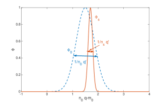
Figure 8: Cartoon of scale separation between TAE and eDW, with the dashed curve being the sketched parallel mode structure of a TAE poloidal harmonic, while the solid curve being the parallel mode structure of eDW with much smaller radial width than that of the TAE.

Thus, the nonlinear coupling processes occur in in a narrow region of the eDW localization. Expanding $\delta\phi_{0}=\Phi_{0}(\mathbf{x}_{0})+\tilde{\Phi}_{0}(\mathbf{x}_{s},\mathbf{x}_{0})$ with $\mathbf{x}_{0}=(R/n_{0},r/m_{0},1/n_{0}q^{\prime})$, $\mathbf{x}_{s}=(R/n_{s},r/m_{s},1/n_{s}q^{\prime})$ and $\lvert\tilde{\Phi}_{0}\rvert/\lvert\Phi_{0}\rvert\sim O(\lvert e\delta\phi_{s}/T_{e}\rvert^{2})\ll 1$, equation (82) becomes, after averaging over $\mathbf{x}_{s}$ scale,

$$\tau b_{0}\epsilon_{A0}\Phi_{0}=\left\langle\left(\frac{\Lambda^{s}_{0}}{2\omega_{0}}\right)^{2}\beta^{+}_{0}\delta\phi^{*}_{s}\frac{\beta_{+}}{\tau b_{+}\epsilon_{A+}}\delta\phi_{s}\right\rangle_{s}\Phi_{0}+\delta\phi_{-}\ \mbox{contribution},$$ (83)

with $\langle\cdots\rangle_{s}$ denoting averaging over eDW scales

$$\langle(\cdots)\lvert\delta\phi_{s}\rvert_{s}\rangle_{s}\equiv\lvert A_{n_{s}}\rvert^{2}\left(\int^{\infty}_{\infty}dz_{s}\lvert\Phi_{s}(z_{s})\rvert^{2}\right)^{-1}\int^{\infty}_{\infty}dz_{s}(\cdots)\lvert\Phi_{s}(z_{s})\rvert^{2}.$$ (84)

Equation (83) can then be solved noting that the absorption due to $\mbox{Im}(1/\epsilon_{A+})$ can be expressed as $\mbox{Im}(1/\epsilon_{A+})=-\pi\delta(\epsilon_{A+})\simeq-(\pi/4\sigma_{*+})\delta(z^{2}_{s}-z^{2}_{+})$ with $z^{2}_{+}=(1-\omega_{*i}/\omega)_{+}(1-\Gamma_{+})(\omega/\omega_{A})^{2}_{+}/(b_{+}\sigma_{*+})$. This implies that KAW are absorbed locally. Thus, expanding $\beta_{+}$ with respect to $b_{s}$ noting the two spatial scale separation $k^{2}_{\perp+}\simeq k^{2}_{\perp s}+2k_{rs}k_{r0}$, and properly reinstating the lower KAW contribution, one obtains,

$$\tau b_{0}\left[\epsilon_{A0}+i\nu(k_{r0}\rho_{i})^{2}\right]\Phi_{0}=0,$$ (85)

with $\nu=\nu_{+}+\nu_{-}$, and

$$\nu_{\pm}\simeq\pi\left(\frac{\Omega_{ci}}{\omega_{0}}\right)^{2}\sum_{n_{s}}\lvert A_{n_{s}}\rvert^{2}\left[\left(\tau+\frac{\sigma_{s}}{2\Gamma_{s}}\right)\frac{\partial\Gamma_{s}}{\partial b_{\theta s}}\right]^{2}\frac{b_{\theta s}\hat{s}^{2}}{\sigma^{2}_{\pm s}z_{\pm}}\left\lvert\frac{\partial\Phi_{s}}{\partial z_{s}}\right\rvert^{2}_{z_{\pm}}.$$ (86)

Equation (85) can be solved perturbatively in ballooning space, $\eta$. Letting $\hat{\Phi}_{0}(\eta)$ being the lowest order linear eigenmode satisfying $\hat{b}_{0}\hat{\epsilon}_{A0}(\eta,\partial_{\eta},\omega_{0})\hat{\Phi}_{0}(\eta)=0$, and expanding $\omega_{0}=\omega_{0,R}+i\gamma_{AD}$ with $\gamma_{AD}$ being the eDW scattering induced test TAE damping rate, equation (85) then gives,

$$\frac{2\gamma_{AD}}{\omega_{0,R}}\left\langle\hat{\Phi}_{0}\hat{b}_{0}\hat{\Phi}_{0}\right\rangle_{\eta}=-\left\langle\hat{\Phi}_{0}\hat{b}_{0}\nu b_{\theta 0}\hat{s}^{2}\eta^{2}\hat{\Phi}_{0}\right\rangle_{\eta},$$ (87)

with $\langle\cdots\rangle_{\eta}\equiv\int^{\infty}_{-\infty}(\cdots)d\eta$. Noting equation (24) for TAE, we obtain

$$\frac{\gamma_{AD}}{\omega_{0,R}}=-\frac{1}{4}\frac{\nu b_{\theta 0}\hat{s}^{2}}{\sqrt{-\Gamma_{l}\Gamma_{u}}}\sim O(10^{-2}-10^{-1}),$$ (88)

as estimated using typical parameters, i.e., $\lvert\Omega_{ci}/\omega_{0,R}\rvert\sim O(10^{2})$, $\sum_{n_{s}}\lvert A_{n_{s}}\rvert^{2}\sim\lvert e\delta\phi_{s}/T_{e}\rvert^{2}\sim O(10^{-4})$, $b_{\theta s}\sim\hat{s}\sim\tau\sim O(1)$ and $4\sqrt{-\Gamma_{l}\Gamma_{u}}\sim O(\epsilon^{2})\sim O(10^{-2}-10^{-1})$. The eDW scattering induced TAE damping rate is comparable to the TAE growth rate due to EP drive LChenRMP2016 , and can significantly reduce or completely suppress TAE fluctuations with sufficiently large eDW intensity. This may imply improved fusion alpha particle confinement in the existence of micro turbulence, and consequently, enhanced thermal plasma heating.

As the nonlinearly generated KAW quasi-modes are dissipated by predominantly electron Landau damping AHasegawaPoF1976 ; LChenRMPP2021 , the resulting electron heating rate can be estimated as

$$\left(\frac{d\beta_{e}}{dt}\right)_{AD}=4\lvert\gamma_{AD}\rvert\left\lvert\frac{\delta B_{\perp}}{B_{0}}\right\rvert^{2}\simeq O(10^{-2}-10^{-1})s^{-1},$$ (89)

which, for typical parameters, can be comparable to the electron heating by alpha particle slowing down, and potentially, contribute significantly to the “anomalous" electron heating in burning plasmas LChenNF2022 .

The present analysis, using TAE scattering by ambient eDW as an example to demonstrate the novel physics of direct cross-scale interaction among meso/macro-scale SAW instabilities and micro-scale DW turbulence, and the obtained results are expected to be, at least qualitatively, applicable to other Alfvén eigenmodes, such as reversed shear Alfvén eigenmode (RSAE), interacting with various branches of DWs, including the physics of finite temperature gradients or trapped electrons. These applications to more realistic scenarios can be investigated for a more detailed understanding of the SAW stabilities and fusion alpha particle confinement in reactors.

4 Summary

Using toroidal Alfvén eigenmode (TAE) nonlinear saturation due to mode-mode coupling as example, we show that, nonlinear gyrokinetic theory is not only efficient, but also necessary to investigate various crucial physics in the nonlinear mode coupling processes of SAW instabilities. This necessity occurs since SAW instabilities often have a small scale structure associated with the SAW continuum related to equilibrium magnetic geometry and plasma nonuniformity of magnetically confined fusion devices. The nonlinear coupling is, thus, dominated through perpendicular scattering LChenEPL2011 . Three main processes developed in the past decade are briefly reviewed, i.e., the zonal field structure generation by TAE LChenPRL2012 , TAE spectral cascading due to ion induced scattering TSHahmPRL1995 ; ZQiuNF2019a , and cross-scale interaction with electron drift wave (eDW) via direct nonlinear interaction LChenNF2022 . The fundamental physics involved in the three processes are reviewed in a pedagogical way, discussing parameter regimes for them to occur and dominate, and state-of-art developments as well as open questions are introduced. These understandings present a road map for a comprehensive and quantitative study of SAW instability spectrum in fusion reactors, and provide guidance for large scale simulations using realistic geometry and plasma parameters.

It is obvious that the nonlinear mode coupling processes reviewed in the present work, and the self-consistent EP transport should be considered on the same footing for the comprehensive understanding nonlinear dynamics and self-organization in burning fusion plasmas. There exists a general theoretical framework that addresses the former wave-wave coupling processes, which can be described by the nonlinear radial envelope equation in the form of a nonlinear Schr$\ddot{o}$dinger equation. Meanwhile, the latter nonlinear wave-particle interactions and ensuing EP transport may be described by the Dyson-Schr$\ddot{o}$dinger model, providing a general theoretical framework for SAW nonlinear dynamics and EP transport in burning plasmas FZoncaNJP2015 ; LChenRMP2016 ; FZoncaJPCS2021 ; MFalessiPoP2019 ; MFalessiNJP2023 .

Declarations

• Conflict of interest

  The authors have no conflicts to disclose.

• Data availability

  The data that support the findings of this study are available from the corresponding author upon reasonable request.

References

- \bibcommenthead
- (1) Alfvén, H.: Existence of electromagnetic-hydrodynamic waves. Nature 150(3805), 405–406 (1942)
- (2) Tomabechi, K., Gilleland, J.R., Sokolov, Y.A., Toschi, R., Team, I.: Iter conceptual design. Nuclear Fusion 31(6), 1135 (1991)
- (3) Wan, Y., Li, J., Liu, Y., Wang, X., Chan, V., Chen, C., Duan, X., Fu, P., Gao, X., Feng, K., et al.: Overview of the present progress and activities on the cfetr. Nuclear Fusion 57(10), 102009 (2017)
- (4) Fasoli, A., Gormenzano, C., Berk, H.L., Breizman, B., Briguglio, S., Darrow, D.S., Gorelenkov, N., Heidbrink, W.W., Jaun, A., Konovalov, S.V., Nazikian, R., Noterdaeme, J.-M., Sharapov, S., Shinohara, K., Testa, D., Tobita, K., Todo, Y., Vlad, G., Zonca, F.: Chapter 5: Physics of energetic ions. Nuclear Fusion 47(6), 264 (2007)
- (5) Chen, L., Zonca, F.: Alfvén waves and energetic particles. Review of Modern Physics 88(1), 015008 (2016)
- (6) Grad, H.: Plasmas. Physics Today 22(12), 34 (1969)
- (7) Chen, L., Hasegawa, A.: Plasma heating by spatial resonance of alfven wave. The Physics of Fluids 17(7), 1399–1403 (1974)
- (8) Hasegawa, A., Chen, L.: Kinetic processes in plasma heating by resonant mode conversion of alfvén wave. Physics of Fluids 19(12), 1924–1934 (1976)
- (9) Chen, L., Zonca, F., Lin, Y.: Physics of kinetic alfvén waves: a gyrokinetic theory approach. Reviews of Modern Plasma Physics 5(1), 1–37 (2021)
- (10) Chen, L.: Theory of magnetohydrodynamic instabilities excited by energetic particles in tokamaks. Physics of Plasmas 1(5), 1519 (1994)
- (11) Cheng, C.Z., Chen, L., Chance, M.S.: High-n ideal and resistive shear alfvén waves in tokamaks. Ann. Phys. 161, 21 (1985)
- (12) Chen, L.: On resonant excitation of high-n magnetohydrodynamic modes by energetic/alpha particles in tokamaks. In: SIF (ed.) Theory of Fusion Plasmas, p. 327. Association EUROATOM, Bologna, Italy (1988)
- (13) Fu, G.Y., Van Dam, J.W.: Excitation of the toroidicity induced shear alfvén eigenmode by fusion alpha particles in an ignited tokamak. Physics of Fluids B 1(10), 1949–1952 (1989)
- (14) Wong, K.L., Fonck, R.J., Paul, S.F., Roberts, D.R., Fredrickson, E.D., Nazikian, R., Park, H.K., Bell, M., Bretz, N.L., Budny, R., Cohen, S., Hammett, G.W., Jobes, F.C., Meade, D.M., Medley, S.S., Mueller, D., Nagayama, Y., Owens, D.K., Synakowski, E.J.: Excitation of toroidal alfvén eigenmodes in tftr. Phys. Rev. Lett. 66, 1874–1877 (1991)
- (15) Vlad, G., Zonca, F., Briguglio, S.: Dynamics of alfvén waves in tokamaks. La Rivista del Nuovo Cimento (1978-1999) 22(7), 1 (1999)
- (16) Zonca, F., Chen, L.: Theory on excitations of drift alfvén waves by energetic particles. ii. the general fishbone-like dispersion relation. Physics of Plasmas 21(7), 072121 (2014)
- (17) Todo, Y.: Introduction to the interaction between energetic particles and alfven eigenmodes in toroidal plasmas. Reviews of Modern Plasma Physics 3(1) (2019)
- (18) Chen, L.: Theory of plasma transport induced by low-frequency hydromagnetic waves. Journal of Geophysical Research: Space Physics 104(A2), 2421 (1999)
- (19) Chen, L., Hasegawa, A.: Kinetic theory of geomagnetic pulsations: 1. internal excitations by energetic particles. Journal of Geophysical Research: Space Physics 96(A2), 1503 (1991)
- (20) Berk, H.L., Breizman, B.N.: Saturation of a single mode driven by an energetic injected beam. i. plasma wave problem. Physics of Fluids B 2(9), 2226 (1990)
- (21) Berk, H.L., Breizman, B.N.: Saturation of a single mode driven by an energetic injected beam. ii. electrostatic universal destabilization mechanism. Physics of Fluids B 2(9), 2235 (1990)
- (22) Berk, H.L., Breizman, B.N.: Saturation of a single mode driven by an energetic injected beam. iii. alfvén wave problem. Physics of Fluids B 2(9), 2246 (1990)
- (23) O’Neil, T.: Collisionless damping of nonlinear plasma oscillations. Physics of Fluids 8(12), 2255–2262 (1965)
- (24) Zonca, F., Chen, L., Falessi, M., Qiu, Z.: Nonlinear radial envelope evolution equations and energetic particle transport in tokamak plasmas. Journal of Physics: Conference Series 1785(1), 012005 (2021)
- (25) Zonca, F., Chen, L., Briguglio, S., Fogaccia, G., Vlad, G., Wang, X.: Nonlinear dynamics of phase space zonal structures and energetic particle physics in fusion plasmas. New Journal of Physics 17(1), 013052 (2015)
- (26) Falessi, M.V., Zonca, F.: Transport theory of phase space zonal structures. Physics of Plasmas 26(2), 022305 (2019)
- (27) Falessi, M., Chen, L., Qiu, Z., Zonca, F.: Nonlinear equilibria and transport processes in burning plasmas. to be submitted to New Journal of Physics (2023)
- (28) Zonca, F., Chen, L., Briguglio, S., Fogaccia, G., Milovanov, A.V., Qiu, Z., Vlad, G., Wang, X.: Energetic particles and multi-scale dynamics in fusion plasmas. Plasma Physics and Controlled Fusion 57(1), 014024 (2015)
- (29) Wang, X., Briguglio, S., Chen, L., Di Troia, C., Fogaccia, G., Vlad, G., Zonca, F.: Nonlinear dynamics of beta-induced alfvén eigenmode driven by energetic particles. Phys. Rev. E 86, 045401 (2012)
- (30) Zhang, H.S., Lin, Z., Holod, I.: Nonlinear frequency oscillation of alfvén eigenmodes in fusion plasmas. Phys. Rev. Lett. 109, 025001 (2012)
- (31) Yu, L., Zonca, F., Qiu, Z., Chen, L., Chen, W., Ding, X., Ji, X., Wang, T., Wang, T., Ma, R., et al.: Experimental evidence of nonlinear avalanche dynamics of energetic particle modes. Europhysics Letters 138(5), 54002 (2022)
- (32) Chen, L., Zonca, F.: On nonlinear physics of shear alfvén waves. Physics of Plasmas 20(5), 055402 (2013)
- (33) Wang, T., Qiu, Z., Zonca, F., Briguglio, S., Fogaccia, G., Vlad, G., Wang, X.: Shear alfvén fluctuation spectrum in divertor tokamak test facility plasmas. Physics of Plasmas 25(6), 062509 (2018)
- (34) Ren, Z., Chen, Y., Fu, G., Wang, Z.: Stability of alfvén eigenmodes in the china fusion engineering test reactor. Nuclear Fusion 60(1), 016009 (2020)
- (35) Chen, L., Zonca, F.: Gyrokinetic theory of parametric decays of kinetic alfvén waves. Europhysics Letters 96(3), 35001 (2011)
- (36) Sagdeev, R.Z., Galeev, A.A.: Nonlinear Plasma Theory [by] R.Z. Sagdeev and A.A. Galeev: Rev. and Edited by T.M. O’Neil [and] D.L. Book. Frontiers in physics. W.A. Benjamin, New York (1969)
- (37) Hahm, T.S., Chen, L.: Nonlinear saturation of toroidal alfvén eigenmodes via ion compton scattering. Phys. Rev. Lett. 74, 266 (1995)
- (38) Qiu, Z., Chen, L., Zonca, F.: Gyrokinetic theory of the nonlinear saturation of a toroidal alfvén eigenmode. Nuclear Fusion 59(6), 066024 (2019)
- (39) Rosenbluth, M.N., Hinton, F.L.: Poloidal flow driven by ion-temperature-gradient turbulence in tokamaks. Phys. Rev. Lett. 80, 724–727 (1998)
- (40) Chen, L., Lin, Z., White, R.: Excitation of zonal flow by drift waves in toroidal plasmas. Physics of Plasmas 7(8), 3129–3132 (2000)
- (41) Chen, L., Zonca, F.: Nonlinear excitations of zonal structures by toroidal alfvén eigenmodes. Phys. Rev. Lett. 109, 145002 (2012)
- (42) Frieman, E.A., Chen, L.: Nonlinear gyrokinetic equations for low-frequency electromagnetic waves in general plasma equilibria. Physics of Fluids 25(3), 502–508 (1982)
- (43) Kieras, C., Tataronis, J.: The shear alfvén continuous spectrum of axisymmetric toroidal equilibria in the large aspect ratio limit. Journal of Plasma Physics 28(3), 395 (1982)
- (44) Brizard, A.J., Hahm, T.S.: Foundations of nonlinear gyrokinetic theory. Rev. Mod. Phys. 79, 421 (2007)
- (45) Sugama, H.: Modern gyrokinetic formulation of collisional and turbulent transport in toroidally rotating plasmas. Reviews of Modern Plasma Physics 1(1), 9 (2017)
- (46) Todo, Y., Berk, H., Breizman, B.: Nonlinear magnetohydrodynamic effects on alfvén eigenmode evolution and zonal flow generation. Nuclear Fusion 50(8), 084016 (2010)
- (47) Qiu, Z., Chen, L., Zonca, F.: Effects of energetic particles on zonal flow generation by toroidal alfvén eigenmode. Physics of Plasmas (1994-present) 23(9), 090702 (2016)
- (48) Chen, L., Lin, Z., White, R.B., Zonca, F.: Nonlinear zonal dynamics of drift and drift-alfvén turbulence in tokamak plasmas. Nuclear fusion 41(6), 747 (2001)
- (49) Chen, L., Qiu, Z., Zonca, F.: On scattering and damping of toroidal alfvén eigenmode by drift wave turbulence. Nuclear Fusion 62(9), 094001 (2022)
- (50) Citrin, J., Jenko, F., Mantica, P., Told, D., Bourdelle, C., Garcia, J., Haverkort, J., Hogeweij, G., Johnson, T., Pueschel, M.: Nonlinear stabilization of tokamak microturbulence by fast ions. Physical review letters 111(15), 155001 (2013)
- (51) Di Siena, A., Görler, T., Poli, E., Navarro, A.B., Biancalani, A., Jenko, F.: Electromagnetic turbulence suppression by energetic particle driven modes. Nuclear Fusion 59(12), 124001 (2019)
- (52) Mazzi, S., Garcia, J., Zarzoso, D., Kazakov, Y.O., Ongena, J., Dreval, M., Nocente, M., Štancar, Ž., Szepesi, G., Eriksson, J., et al.: Enhanced performance in fusion plasmas through turbulence suppression by megaelectronvolt ions. Nature Physics 18(7), 776–782 (2022)
- (53) Lin, Z., Hahm, T.S., Lee, W.W., Tang, W.M., White, R.B.: Turbulent transport reduction by zonal flows: Massively parallel simulations. Science 281(5384), 1835–1837 (1998)
- (54) Zonca, F., White, R.B., Chen, L.: Nonlinear paradigm for drift wave–zonal flow interplay: Coherence, chaos, and turbulence. Physics of Plasmas 11(5), 2488–2496 (2004)
- (55) Diamond, P.H., Itoh, S.-I., Itoh, K., Hahm, T.S.: Zonal flows in plasma: a review. Plasma Physics and Controlled Fusion 47(5), 35 (2005)
- (56) Spong, D., Carreras, B., Hedrick, C.: Nonlinear evolution of the toroidal alfvén instability using a gyrofluid model. Physics of plasmas 1(5), 1503 (1994)
- (57) Zonca, F., Lin, Y., Chen, L.: Spontaneous excitation of convective cells by kinetic alfvén waves. Europhysics Letters 112(6), 65001 (2015)
- (58) Qiu, Z., Chen, L., Zonca, F.: Nonlinear excitation of finite-radial-scale zonal structures by toroidal alfvén eigenmode. Nuclear Fusion 57(05), 056017 (2017)
- (59) Qiu, Z., Chen, L., Zonca, F.: Spontaneous excitation of geodesic acoustic mode by toroidal alfvén eigenmodes. Europhysics Letters 101(3), 35001 (2013)
- (60) Qiu, Z., Chen, L., Zonca, F.: Fine radial structure zonal flow excitation by beta-induced alfvén eigenmode. Nuclear Fusion 56(10), 106013 (2016)
- (61) Zhang, H., Lin, Z.: Nonlinear generation of zonal fields by the beta-induced alfvén eigenmode in tokamak. Plasma Science and Technology 15(10), 969 (2013)
- (62) Wei, S., Wang, T., Chen, N., Qiu, Z.: Nonlinear reversed shear alfvén eigenmode saturation due to spontaneous zonal current generation. Journal of Plasma Physics 87(5), 905870505 (2021)
- (63) Heidbrink, W.W., Gorelenkov, N.N., Luo, Y., Van Zeeland, M.A., White, R.B., Austin, M.E., Burrell, K.H., Kramer, G.J., Makowski, M.A., McKee, G.R., Nazikian, R.: Anomalous flattening of the fast-ion profile during alfvén-eigenmode activity. Phys. Rev. Lett. 99, 245002 (2007)
- (64) Biancalani, A., Bottino, A., Siena, A.D., Gurcan, O., Hayward-Schneider, T., Jenko, F., Lauber, P., Mishchenko, A., Morel, P., Novikau, I., Vannini, F., Villard, L., Zocco, A.: Gyrokinetic investigation of alfvén instabilities in the presence of turbulence. Plasma Physics and Controlled Fusion 63(6), 065009 (2021)
- (65) Hahm, T.S.: Ion heating from nonlinear landau damping of high mode number toroidal alfvén eigenmodes. Plasma Science and Technology 17(7), 534 (2015)
- (66) Fisch, N.J., Herrmann, M.C.: Utility of extracting alpha particle energy by waves. Nuclear Fusion 34(12), 1541 (1994)
- (67) Fisch, N.J., Rax, J.-M.: Interaction of energetic alpha particles with intense lower hybrid waves. Phys. Rev. Lett. 69, 612–615 (1992)
- (68) Qiu, Z., Chen, L., Zonca, F., Chen, W.: Nonlinear decay and plasma heating by a toroidal alfvén eigenmode. Phys. Rev. Lett. 120(13), 135001 (2018)
- (69) Qiu, Z., Chen, L., Zonca, F., Chen, W.: Nonlinear excitation of a geodesic acoustic mode by toroidal alfvén eigenmodes and the impact on plasma performance. Nuclear Fusion 59(6), 066031 (2019)
- (70) Wei, S., Wang, T., Chen, L., Zonca, F., Qiu, Z.: Core localized alpha-channeling via low frequency alfvén mode generation in reversed shear scenarios. Nuclear Fusion 62(12), 126038 (2022)
- (71) Wang, T., Wang, X., Briguglio, S., Qiu, Z., Vlad, G., Zonca, F.: Nonlinear dynamics of shear alfvén fluctuations in divertor tokamak test facility plasmas. Physics of Plasmas 26(1), 012504 (2019)
- (72) Brizard, A.J.: Nonlinear gyrokinetic vlasov equation for toroidally rotating axisymmetric tokamaks. Physics of Plasmas 2(2), 459–471 (1995)
- (73) Fu, G., Cheng, C.: Excitation of high-n toroidicity-induced shear alfvén eigenmodes by energetic particles and fusion allpha-particles in tokamaks. Physics of Fluids B - Plasma Physics 4(11), 3722 (1992)
- (74) Chen, L., Qiu, Z., Zonca, F.: Parity-breaking parametric decay instability of kinetic alfvén waves in a nonuniform plasma. Physics of Plasmas 29(5), 050701 (2022)
- (75) Cheng, Z., Shen, K., Chen, L., Zonca, F., Qiu, Z.: Effects of plasma non-uniformity on toroidal Alfvén eigenmode nonlinear saturation via ion induced scattering (2023)
- (76) Chen, L., Qiu, Z., Zonca, F.: On nonlinear scattering of drift wave by toroidal alfvén eigenmode in tokamak plasmas. submitted to Nuclear Fusion (2023)
- (77) Horton, W.: Drift waves and transport. Rev. Mod. Phys. 71, 735–778 (1999)
- (78) Zhang, W., Lin, Z., Chen, L.: Transport of energetic particles by microturbulence in magnetized plasmas. Phys. Rev. Lett. 101(9), 095001 (2008)
- (79) Feng, Z., Qiu, Z., Sheng, Z.: The mechanism of particles transport induced by electrostatic perturbation in tokamak. Physics of Plasmas 20(12), (2013)
- (80) Günter, S., Conway, G., Fahrbach, H.-U., Forest, C., Muñoz, M.G., Hauff, T., Hobirk, J., Igochine, V., Jenko, F., Lackner, K., et al.: Interaction of energetic particles with large and small scale instabilities. Nuclear Fusion 47(8), 025 (2007)
- (81) Suzuki, T., Ide, S., Oikawa, T., Fujita, T., Ishikawa, M., Seki, M., Matsunaga, G., Hatae, T., Naito, O., Hamamatsu, K., et al.: Off-axis current drive and real-time control of current profile in jt-60u. Nuclear Fusion 48(4), 045002 (2008)
- (82) Heidbrink, W., Park, J.M., Murakami, M., Petty, C., Holcomb, C., Van Zeeland, M.: Evidence for fast-ion transport by microturbulence. Physical review letters 103(17), 175001 (2009)
- (83) Zweben, S., Budny, R., Darrow, D., Medley, S., Nazikian, R., Stratton, B., Synakowski, E., Taylor, G.: Alpha particle physics experiments in the tokamak fusion test reactor. Nucl. Fusion 40, 91 (2000)
- (84) Tardini, G., Hobirk, J., Igochine, V., Maggi, C., Martin, P., McCune, D., Peeters, A., Sips, A., Stäbler, A., Stober, J., et al.: Thermal ions dilution and itg suppression in asdex upgrade ion itbs. Nuclear fusion 47(4), 280 (2007)
- (85) Bourdelle, C., Hoang, G., Litaudon, X., Roach, C., Tala, T.: Impact of the parameter on the microstability of internal transport barriers. Nuclear fusion 45(2), 110 (2005)
- (86) Citrin, J., Mantica, P.: Overview of tokamak turbulence stabilization by fast ions. Plasma Physics and Controlled Fusion 65(3), 033001 (2023)
- (87) Di Siena, A., Gorler, T., Poli, E., Banon Navarro, A., Biancalani, A., Bilato, R., Bonanomi, N., Novikau, I., Vannini, F., Jenko, F.: Nonlinear electromagnetic interplay between fast ions and ion-temperature-gradient plasma turbulence. Journal of Plasma Physics 87(2), 555870201 (2021)