Answer to the referee’s report

We thank the referee for his/her review report which enabled us to improve significantly our manuscript. Here are our answers to the comments:

The manuscript analyses CME simulations using the heliospheric model EUHFORIA in several different setups to analyse how CME propagates/evolves in different conditions. It is well structured, with fair references and may possibly offer significant new results within the scope of the journal after some issues are clarified. These are highlighted below.

1.Why use GONG in minimum activity and GONG adapt in maximum? Why not use GONG in both (to be consistent)? How do you know how much difference between 2 runs is coming from max/min activity and how much from using different magnetograms?

Our reply: GONG-ADAPT magnetic maps are only available after 2010, so because the minimum of activity case was selected in 2008, it was not possible to use GONG-ADAPT for the minimum case. We initially tried the simulation at maximum of activity with the GONG map, but it produced spurious structures at the outer boundary conditions that we feared would interfere with the CME and thus produce unrealistic results (see example on figure 1 of this document. GONG maps are known to perform less well than GONG-ADAPT at maximum of activity, so we preferred having a difference in the magnetograms rather than a non-physical run. We will have an upcoming study dedicated to the differences induced by different magnetograms that will focus on this specific point, but this is beyond the scope of this study. Also, from figure 2 of this answer, it is very clear that the difference created by taking a minimum vs. a maximum of activity is going to produce a greater effect than taking two different magnetograms from the same date.

We have changed Figure 1 in the manuscript to now include all 3 maps, and have made these points more clear in the manuscript (lines 260-269): This causes a difference in the provider and thus the processing of the input map. However, it guarantees that the final solution does not suffer from numerical artifacts. We also show in Figure 1 the difference between GONG and GONG-ADAPT at maximum of activity. We can see that there is a difference in amplitude for the most intense active region, sometimes a difference in polarity for the quiet Sun and a different method for filling the solar poles. However, the general structure is still very similar, and these differences are still less than the difference between minimum and maximum of activity. This means that the differences we may see in the final CME solutions are indeed mainly due to the difference in solar activity. We will dedicate a specific study on the impact of the input magnetic map on the final CME solution, but for now it is out of the scope of this paper.

Figure 1: Visualization of a test simulation using the GONG map for the maximum of activity case. We show the ecliptic view on the left panel and the meridional view on the right panel. In the right panel, we can see an elongated north-south transversal structure of high density that did not disappear after 14 days of relaxation. This type of structure is the reason why we switched to GONG-ADAPT maps for maximum of activity.

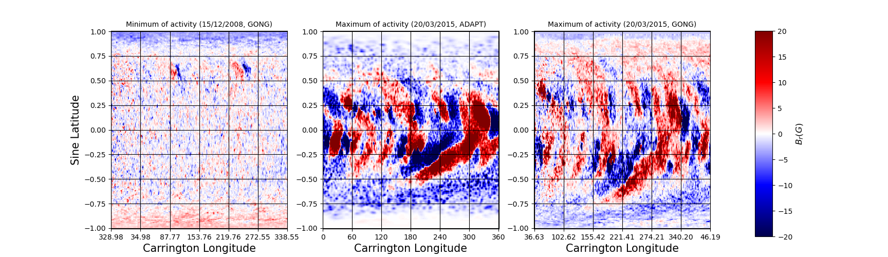
Figure 2: Comparison between the different magnetic maps used as inputs. The left panel is the GONG map for minimum of activity (15th of December 2008), the middle panel is the GONG-ADAPT map for maximum of activity (20th of March 2015), and the right panel is the GONG map for maximum of activity. We can see a greater difference between the left and middle panel, than the middle and right panel.

2. Line 282/283: What is Radius (set to 15Rsun)? Is this CME radius (if so at which height)? What is the motivation for using this value, how does it compare to observations?

Our reply: The radius we describe here is the radius of the cone/spheromak CME (both assumed spherical) at the injection point, which is 0.1 au. This has been made clearer in the manuscript: which then defines an initial radius at the injection point (lines 214-215), initial radius at injection (lines 299-300).

Based on previous studies conducted on EUHFORIA, it is a standard value that guarantees visible measurements at Earth. This has been made clearer in the manuscript: This value corresponds to an average of the values found by GCS fitting for the events studied in Scolini2019, which were 10.5, 14.5, 16.8 and 18.0 solar radii (lines 299-301).

3. In EUHFORIA input description you state that spheromak uses the same input as Cone + magnetic properties. Why then do you not use the same input in your study but shift to Donki input for Cone model? The speed is almost double and temperature 3x larger!? It’s like looking at two completely different CMEs, not really comparable?

Our reply: We agree that our formulation was misleading. What we meant is that the physical nature and meaning of the input parameters is the same, but the values have to be adjusted. As explained in Scolini2019 (and in our section 5), the radial speed of the CME is the same as its 3D speed in the case of a cone CME, but not a spheromak (where you also have to take into account the expansion speed). To have a CME of similar geo-effectiveness, we then need to divide the speed by around two. This was the case is Scolini2019, where they compared a cone and spheromak run for the 12th of July 2012 event : the cone CME has an input speed of 1266 km/s, and the spheromak CME of 763 km/s (because now we need to subtract the expansion speed of the CME). We performed an initial run with the same CME speed for the cone CME, and it was barely visible at Earth in the 1D physical quantities signatures.

This has been made more clear in the manuscript sooner: This means that the total speed of the CME $v_{3D}$ can be decomposed into two components: the radial speed $v_{rad}$ and the expansion speed $v_{exp}$. In our case, we prescribe only the radial speed at the injection point (lines 224-226), It requires the same physical input parameters as the cone model, plus three additional magnetic parameters (lines 226-227), The lower initial speed is due to the fact that we prescribe only the input radial speed, which is equal to the full 3D speed inferred from observations for a cone model ($v_{rad}=v_{3D}$), but equal to the difference between the 3D speed and the expansion speed for a spheromak ($v_{rad}=v_{3D}-v_{exp}$). For the reference case, the CME geometric parameters were derived using a GCS model (Graduated Cylindrical Shell model, see Thernisien2009; Thernisien2011), which gave a full 3D speed $v_{3D}$ of 1266 or 1352 km/s depending on the fitting. The expansion speed of the CME is derived using empirical relations from DalLago2003 and Schwenn2005, which is an alternative when 3D reconstruction of the event is not possible due to a single spacecraft configuration for the observation (more details in Scolini2019). These relations give: $v_{rad}=0.43v_{3D}$ in the case of a spheromak, which explains the difference in input speed of a factor close to 2. The DONKI database values are thus consistent with the values obtained from Scolini2019. This is explained in more details in Scolini2019. (lines 307-318), but we recall from section 3.2 that the full 3D speed is actually the same (line 498).

4. Appendix B, lines 679-686: From how is now written the criteria for shock using B is 10 times increase of B? Is this correct? That means for a typical ambient magnetic field (upstream) of 5 nT downstream magnetic field (in the sheath) would have to be 50 nT, which is definitely much higher than typical observations. The criteria that is referenced being used by Scolini et al. (Bthreshold = 1.2 nT) sounds more reasonable, but it is stated that the values are adjusted to obtain most logical results with eye comparison. So in the end it is not clear whether a strict criteria for threshold is used on all examined cases (and if so, what criteria this is) or the borders were determined visually for each case, thus the thresholds are different for each case (if so these should be written somewhere). Please elaborate.

Our reply: We agree that our formulation was misleading. First it needs to be clear that, although we are using a similar criteria that Scolini2021_radial, we apply it to a different configuration: in their cases, they compare a wind-only simulation to a wind+CME simulation; in our cases, we use only one wind+CME simulation, and we compare the current instant with a past instant. Also, they used only one specific background which was set for maximum of activity, and only one modeling of the ICME which was a spheromak. That is why we cannot have the same values as in Scolini2021_radial for all our cases. We could have used more refined criteria for each case, but here we wanted to go for a generic criterion that would work for all our cases.

Still, we have tried to get values closer to theirs, and succeeded. The new thresholds are: $v_{thresh}=30$ km/s, $n_{thresh}=1.5$, $B_{thresh}=1.5$, for $\Delta t=10$ (with 10 minutes between each output, this means an interval of around 1.6 hours). The previous difference lied in the fact that our $\Delta t$ was large, while Scolini2021_radial compared quantities at the same instant, which explains why we have reduced it. We also have a case at minimum of activity, which means the Earth is closer to the HCS and as a result, values of the magnetic field do decrease significantly locally. Hence the ratio of 20 was achieved, but because of these low values close to 0. We have now excluded them from the shock research, and this gave better results in closer agreement with Scolini2021_radial.

We have updated all corresponding figures and tables with this new criterion, and made this clearer in the manuscript: Scolini2021_radial set their own thresholds to the following values: $v_{thresh}=20$ km/s, $n_{thresh}=1.2$, $B_{thresh}=1.2$. However, these were for a comparison between the CME run and the corresponding wind-only simulation, which means they used a wind model for reference. In our case, we use only one CME run and compare present time with previous time data. This means that our threshold values need to be different. We have thus adjusted these values by trying different combinations, and selected the most robust and efficient ones. These final parameter values are: $\Delta t=10$ (with 10 minutes between each output, this means an interval of around 1.6 hours), $v_{thresh}=30$ km/s, $n_{thresh}=1.5$, $B_{thresh}=1.5$ ($n_{thresh}$ and $B_{thresh}$ do not have units because they are ratios). Since we have a minimum of activity configuration, the HCS is close to the equatorial place and as a result, the magnetic field can become very close to 0 locally, producing false detection of the shock because of these low values. To avoid this, we have set an additional threshold of 1 G for the local magnetic field. (lines 707-720).

Concerning the following sentence: "We have adjusted these values to our cases to obtain the most logical results with eye-comparison", we agree that it was confusing. What we meant to say is that every case has also been checked visually by the authors to make sure our automatic threshold did not produce unrealistic boundaries. The threshold parameters are the same for every case, as explained now in the manuscript: On top of the automatic selection given by this criterion, systematic visual verification has been made to ensure the validity of the results (lines 719-720).

5. Appendix B, lines 691-692: "If the $\beta$ parameter is overall smaller than 0.2" this low beta value for ambient solar wind sounds quite weird. Mag. field has to be very large in those cases and/or temperature and density very low. Please refer to some examples and why/how this would be in the ’normal’ solar wind.

Our reply: Here we are not referring to the value inside the solar wind, we are referring to the value inside the CME ejecta, as can be seen in Figure 16.

We have also provided a table (Table 2) with all the values used for $\beta$ for the border selection of the magnetic ejecta to make it more clear: For our cases, it is the value of 0.1 which usually gives the best results. However, we sometimes had to adjust it manually in order to get a ME selection consistent with the other physical quantities. For clarity, we have indicated the value of $\beta$ used for the border selection in table 3 (lines 724-727).

6. 342/343: "the opposite side of Earth" with respect to what? Solar equator?

Our reply: We agree that our formulation was confusing. We meant behind the Sun as viewed from Earth, so that these structures would not affect the Earth spatial environment. We have rephrased it accordingly: …any large-scale structures (such as high-speed streams where the wind speed reaches 500 km/s or more) is not Earth directed and thus not geo-effective… (lines 371-372).

7. Figure 7: is Earth plotted in all three views? I cannot recognize it, please use different color.

Our reply: Yes, Earth is always plotted at 1 au in the HEEQ frame in blue. We have added a white contour to make it more visible in all relevant figures.

8. Figure 8: By looking at the Figure I would not say that a clear shock arrival or ME is observed in all cases. Also I disagree that CMEs produced similar 1D profiles at Earth, please support this claim. Please also plot magnetic field and temperature to give more credibility to your border selection and to help understand the behavior of the beta parameter. Also, change the y-axis for beta for sol max, as it looks as a flat line. The border where MEmin ends seems to be put at beta>5, much higher than any threshold mentioned in appendix B - can you explain why? As a result of your method of border selection the standoff distance in sol max is more than 5x greater than in the sol min for the same CME - how do you explain this and how does this compare to real observations?

Our reply: We have added words of caution and discussed the visibility of the shock: Because it is a cone CME, the detection of the ICME and its internal borders is a bit more challenging due to the lack of internal magnetic structure, but the global overview of all these physical quantities allow us to make estimations. The initial shock of the ICME is visible in velocity, but more clear in density and in the total magnetic field (lines 443-446).

We have also specified that the similarity we discussed was in particular focused on the speed profile: Although the two CMEs have very different 3D structures, their 1D profile at Earth are actually not so different in density, temperature, and especially radial velocity (lines 441-443).

We have added the temperature and total magnetic field in all the relevant figures (8, 10, 11 and 13).

We have adjusted the y-axis of the last panel as recommended.

We have added a new table in the appendix in order to clarify the values of $\beta$ used in each case for the border selection (Table 3).

Finally, in this paper our goal is not to compare to observations, we aim at performing a theoretical study in order to assess and quantify the effect of the activity level of the Sun on the propagation of CMEs. Relating these results to real cases would be the object of an entirely new paper. What we can say is that for magnetized cases studied previously in Scolini2021_radial, we expect to use values of $\beta$ between 0.1 and 1, which is the case here.

9. Figures 10, 11, 13: Please also plot magnetic field and temperature to give more credibility to your border selection and to help understand the behavior of the beta parameter. Also, change the y-axis for beta, as it looks as a flat line (perhaps use a log scale)?

Our reply: We have made the recommended changes.

10. It would be good to see a table summarizing arrival times of shocks and ejectas, as well as sheath and ejecta duration for solar min and max and two helicities before making conclusions about possible influence of handedness on the propagation. It seems not only arrival times of shock/ME change but also sheath and ME duration. How much is this influenced by thresholds used to define borders (this is especially important since, as I expressed earlier, there might be some doubts related to border selection). Which handedness results in earlier shock arrival and which in earlier ME arrival (this was not very clearly written in the text)? What is the possible explanation? (simply stating that one is faster and thus arrives earlier is not really explanation, why would difference in handedness cause difference in speed of ME or shock?)

Our reply: We thank the referee for this suggestion, and have added the corresponding table summarizing our arrival times of shock, sheath and ejecta (Table 2). As explained previously, the criteria used is the same for every model, hence the result is indeed in the simulation and not the visualization. We have highlighted in the text our possible explanation, which could be both numerical (the spheromak CME at negative handedness follows a quick reconnection at injection that accelerates it, as seen in figure 14) and physical (following the results of Chané et al. 2005 and 2006, it has been shown before that the handedness can have such an effect for a minimum of activity configuration, because it causes an anti-aligned CME configuration). All of these explanations can be found in section 6.3, supported by Figure 14.

11. Also, I suppose it could be important to see in which polarity the CME is dominantly moving (as I seem to remember these were not the same for sol min and max conditions you set)?

Our reply: The information about the polarity in which the CME propagate is already available in Figures 4 and 6 (last panel for both), and is also pointed out in the text. We have however added movies to the material attached to the paper, and in these movies we can see the velocity, density and magnetic field polarity in which the ICME propagates for all cases.