Bubbletrons

Abstract

In cosmological first-order phase transitions (PT) with relativistic bubble walls, high-energy shells of particles generically form on the inner and outer sides of the walls. Shells from different bubbles can then collide with energies much larger than the PT or inflation scales, and with sizable rates, realising a ‘bubbletron’. As an application, we calculate the maximal dark matter mass $M_{\rm DM}$ that can be produced from shell collisions in a $U(1)$ gauge PT, for scales of the PT $v_{\phi}$ from MeV to $10^{16}$ GeV. We find for example $M_{\rm DM}\sim 10^{6}/10^{11}/10^{15}$ GeV for $v_{\phi}\sim 10^{-2}/10^{3}/10^{8}$ GeV. The gravity wave signal sourced at the PT then links Pulsar Timing Arrays with the PeV scale, LISA with the ZeV one, and the Einstein Telescope with grand unification.

I Introduction

Particle accelerators of different sorts continue to play a prominent role in physics. Laboratory accelerators gave us an immense amount of knowledge about the fundamental building blocks of Nature. Astrophysical accelerators (supernovae, active galactic nuclei, …), furthermore, contributed not only to our understanding of the universe, but also shaped the way it looks. In this letter we point out that cosmological particle accelerators may also have existed, if a first order phase transition (PT) took place in the early universe, and we begin to quantitatively explore their implications.

Along with the electroweak (EW) and QCD transitions, known to be crossovers in the Standard Model (SM) [1, 2], one or more first order phase transitions may have taken place in the first second after inflation. They are indeed commonly predicted in several motivated extensions of the SM, such as extra-dimensional [3], confining [4, 5], or supersymmetric models [6], and solutions to the strong CP [7, 8], flavour [9], or neutrino mass problems [10]. Independently of where they come from, such early universe phase transitions may have far reaching consequences through the possible cosmological relics they can leave behind, e.g. primordial black holes [11, 12, 13, 14, 15, 16, 17, 18, 19, 20, 21], topological defects [22, 23, 24, 25, 26], magnetic fields [27, 28, 29, 30, 31, 32, 33], dark matter (DM) [34, 35, 36, 37, 38, 39, 40, 41, 42, 43], the baryon asymmetry [44, 45, 46, 47, 48, 49, 50, 51, 52, 53, 54, 55, 56], together with a background of gravitational waves (GW) [57, 58, 59, 60, 61, 62, 63, 64, 65, 66], to cite just a few.

As the universe expands, sitting in its lowest free energy vacuum, another vacuum may develop at a lower energy due to the fall in temperature, eventually triggering a PT. If a PT is first order then it proceeds via the nucleation of bubbles of broken phase into the early universe bath (see e.g. [67, 68] for reviews), analogously to the PT of water to vapor. Bubble walls that expand with ultrarelativistic velocities store a lot of energy, locally much higher than both the bath temperature and the scale of the PT. Wall interactions with the bath then necessarily accelerate particles to high energies and accumulate them into shells, as first worked out in specific cases in [39, 69, 70, 71]. Collisions of shells from different bubbles constitute a ultra-high-energy collider in the early universe, which we dub ‘bubbletron.’ 

In this letter we initiate a quantitative study of bubbletrons. We review wall velocities in Sec. II and determine the shells’ collision energies in Sec. III, we classify bubbletrons and calculate the resulting production of heavy particles in Sec. IV, apply our findings to heavy DM in Sec. V and correlate them with the GW from the PT in Sec. VI. In Sec. VII we conclude.

II First order phase transitions with fast bubble walls

We consider a cosmological first-order phase transition between two vacuum states with zero-temperature energy density difference $\Delta V=c_{\rm vac}\,v_{\phi}^{4}$, where $c_{\rm vac}\lesssim\mathcal{O}(1)$ is a model-dependent parameter and $v_{\phi}$ is the VEV of the PT order parameter $\phi$ (e.g. a scalar field) in the final vacuum. As the universe expands and cools its temperature falls below the critical temperature $T_{c}$, i.e. when the two minima of the thermal potential have the same free energy density, and the PT becomes energetically allowed. The PT happens around the temperature $T=T_{n}<T_{c}$, defined by the condition $\Gamma(T_{n})=H^{4}(T_{n})$, where $H$ is the Hubble parameter and $\Gamma$ the tunneling rate, per unit volume, between the two vacua. At $T_{n}$ bubbles of the broken phase (i.e. where the order parameter sits in its zero-temperature vacuum) are nucleated and start expanding to eventually fill the universe. The time they take to do so and complete the PT is set by $\beta^{-1}$, with $\beta\equiv(d\Gamma/dt)/\Gamma$, which is shorter than a Hubble time.

The bubble walls are defined as the spherically symmetric regions of space where the background field $\phi$ rapidly varies, from the high-temperature value outside the bubble, to $v_{\phi}$ inside it. The pressure density inside is larger than outside, so the bubbles expand. If friction pressure on the walls is negligible, then they run away with a Lorentz boost $\gamma(R)=R/(3R_{\text{nuc}})$ [69], where $R$ is the bubble radius and $R_{\text{nuc}}\approx T_{n}^{-1}$ is its radius at nucleation, see e.g. [39]. If the walls runaway until colliding, they reach

$$\gamma_{\rm run}=\frac{R_{\rm coll}}{3\,R_{\text{nuc}}}\simeq 2.7\cdot 10^{14}\cdot\frac{T_{\rm n}}{T_{\rm eq}}\,\frac{\rm TeV}{v_{\phi}}\,\frac{1}{(c_{{\rm vac}}g_{b})^{\!\frac{1}{4}}}\frac{20}{\beta/H}$$ (1)

where $R_{\rm coll}\leavevmode\nobreak\ \simeq\leavevmode\nobreak\ (8\pi)^{\!\frac{1}{3}}\beta^{-1}$ is their radius at collision [73], $T_{\rm eq}=(30c_{\rm vac}/(\pi^{2}g_{b}))^{\!\frac{1}{4}}\,v_{\phi}$ is the temperature when the radiation energy density, $\rho_{\rm rad}=g_{b}\pi^{2}T^{4}/30$ with $g_{b}$ the number of relativistic degrees of freedom before the PT, equals $\Delta V$, and we have assumed $T_{n}\leq T_{\rm eq}$ so that $H\simeq\sqrt{c_{{\rm vac}}/3}v_{\phi}^{2}/M_{{\rm Pl}}$.

A number of effects can exert pressure on walls and slow them down. Collisional plasma effects are expected to exert a negligible pressure for $T_{n}\lesssim T_{\rm eq}$ (see e.g. [74, 75, 76, 77]), which is the case we will be interested in. One then enters the so-called ballistic regime, where particle interactions can be neglected. Then, one has pressure from single particles getting a mass across the wall, $\mathcal{P}_{{\rm LO}}=g_{*}\Delta m^{2}\,T_{n}^{2}/24$ [78], with $g_{*}$ the number of degrees of freedom getting an average mass squared $\Delta m^{2}\propto v_{\phi}^{2}$ at the PT. Another pressure that could be relevant in some models, $\mathcal{P}_{{\rm heavy}}$, is that from degrees of freedom heavier than $v_{\phi}$ that couple to the particles that feel the PT [79]. $\mathcal{P}_{{\rm LO}}$ and $\mathcal{P}_{{\rm heavy}}$ are both smaller than $\Delta V$ for $T_{n}^{2}<v_{\phi}^{2}$, up to order-one model-dependent coefficients. In this case, which will be the focus of this letter, the velocity of bubble walls becomes ultrarelativistic.

Ultrarelativistic bubble walls can either run away until they collide with those of other bubbles, or reach a terminal velocity beforehand, set by yet another source of pressure given by the particle emitted by the bath and that get a mass $m$ at wall crossing. If this transition radiation is soft-enhanced, as for emitted gauge bosons, then their pressure grows with $\gamma$ [80]. Its size is enhanced by large logarithms, that have been resummed in [69], which gives the pressure $\mathcal{P}_{{\rm LL}}\simeq\frac{\zeta(3)}{\pi^{4}}g^{2}g_{\rm eff}\,\gamma\,m_{V}\,T_{n}^{3}\log(m_{V}/\mu)$, where $g$ is the gauge coupling, $g_{\rm eff}$ a weighted sum of the radiating degrees of freedom times their charges, $m_{V}$ is the gauge boson mass and $\mu$ a physical IR cut-off. If $\mathcal{P}_{{\rm LL}}(\gamma)$ reaches $\Delta V=c_{{\rm vac}}v_{\phi}^{4}$ before collision, then walls reach a terminal velocity

$$\gamma_{{\rm LL}}\simeq 3.5\cdot 10^{4}\cdot\Big{(}\frac{T_{\rm eq}}{T_{n}}\Big{)}^{\!3}\Big{(}\frac{0.1}{g}\Big{)}^{\!\!3}\Big{(}\frac{c_{{\rm vac}}g_{b}^{3}}{10^{4}}\Big{)}^{\!\!\frac{1}{4}}\frac{10}{g_{\rm eff}\log\!\frac{m_{V}}{\mu}},$$ (2)

where we have chosen $m_{V}=gv_{\phi}$ for definiteness. The typical boost of bubble walls at collision then is

$$\gamma_{{\rm coll}}\simeq\textrm{Min}\big{[}\gamma_{{\rm LL}},\,\gamma_{\rm run}\big{]}.$$ (3)

Large boosts at collision are realised for small gauge coupling $g$, or for large $v_{\phi}/T_{n}$, or in global (rather than gauged) PTs because there $\mathcal{P}_{{\rm LL}}$ does not grow with $\gamma$.

III Shells of particles at the walls

The mechanisms at the origin of the pressures above also cause particles to accumulate into shells, which we list below:

1. Particles acquiring their mass [78, 56];

2. Particles radiated and transmitted in the wall [69];

3. Heavier particles if produced by lighter ones that feel the PT [79, 56, 70];

4. In confining PTs, hadrons from string fragmentation [39];

5. Vectors acquiring a small part of their mass [71];

6. Particles produced by oscillations of the wall $\phi$ [81];

7. In confining PTs, ejecta from string fragmentation [39];

8. Particles radiated and reflected by the wall [69].

Shells 1 to 6 follow the bubble walls, shells 7 and 8 precede them. When bubbles collide, also these shells do. If their constituent particles still have an energy much larger than $v_{\phi}$ by that time, then they realise what we define a ‘bubbletron.’ Whether that happens depends on a number of propagation effects, their study can be model-dependent and pretty complicated, and we are aware of very few attempts at carrying it out in some detail [39, 69, 70]. Accordingly, we have made a novel systematic study of shell propagation, that we present in another paper [82] because its interest goes beyond bubbletrons (for example it could affect GW from PTs), and whose results will be used in this letter.

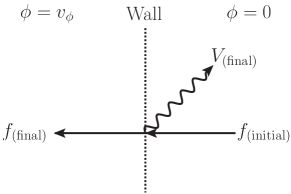
Figure 1: The shell source considered in this letter. Charged particles entering the bubble can radiate a gauge boson which is reflected by the wall back into the false vacuum phase. These gauge bosons form shells propagating in front of the bubble walls.

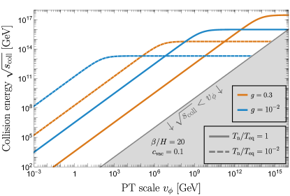
Figure 2: Center-of-mass scattering energies of two gauge bosons radiated and reflected at the walls of different bubbles.

To give a quantitative idea of the center-of-mass energies achievable, let us consider as an example the case of gauge bosons, with mass $m_{V}$, radiated and reflected by the walls (see Fig. 1). If shells free stream until they collide, one has the typical center-of mass collision energy squared (see Fig. 2)

$$s_{\rm coll}\simeq 4\,\gamma_{{\rm coll}}^{2}\,E_{V}^{2}\simeq 0.4\,\gamma_{{\rm coll}}^{2}\,m_{V}^{2}\,,$$ (4)

where $E_{V}$ is the typical energy of a reflected shell particle in the wall frame and we have assumed heads-on collisions for simplicity. In the second equality we have used $E_{V}^{2}\simeq 0.1m_{V}^{2}$, which we computed from the distribution $dP_{V}\propto\frac{dk_{\perp}^{2}}{k_{\perp}^{2}}\frac{dE_{V}}{E_{V}}(\frac{m_{V}^{2}}{m_{V}^{2}+k_{\perp}^{2}})^{2}$ [69], with $k_{\perp}$ the component of $V$ momentum parallel to the wall. Interestingly, collision energies can lie above the scales of both grand unification [83] and inflation [84],

$$\sqrt{s_{\rm coll}}\simeq 1.7\cdot 10^{17}\leavevmode\nobreak\ {\rm GeV}\,g\,\frac{\gamma_{\rm coll}}{\gamma_{\rm run}}\frac{T_{\rm n}}{T_{\rm eq}}\frac{1}{(c_{{\rm vac}}g_{b})^{\!\frac{1}{4}}}\frac{20}{\beta/H}\,.$$ (5)

Let us further consider for simplicity a gauged $U(1)$ with coupling $g$ spontaneously broken by a scalar $\phi$ with charge 1. The condition that shells free stream until collision is realised for small $g$, large $v_{\phi}$, or large $v_{\phi}/T_{n}$, see Fig. 3 and [82]. In that case one obtains collisions at energies much larger than the scale of the PT, and thus potentially than the temperature ever reached by the universe after inflation, opening up the possibility to test such high energies with cosmology.

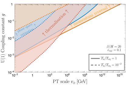
Figure 3: Shells constituted by radiated reflected gauge bosons at a $U(1)$ PT. Free streaming until collision is not realised in the shaded areas, which are an envelope of various effects calculated in [82], like shell thermalisation (dominating for $T_{n}/T_{\rm eq}=10^{-2}$), momentum reversal of shell particles in the wall frame (dominating for $T_{n}/T_{\rm eq}=1$) and saturation of phase space.

IV Shell collision products

We assume that a collision of particles $i$ and $j$ from two different shells produces one much heavier particle $Y$ with cross section times Moeller velocity $\sigma v_{\rm M}|_{ij}(s)$. The probability that a particle $i$ undergoes one such interaction is given by $\int_{\mathcal{\lambda}=0}^{L_{\rm shell}}\frac{d\lambda}{v_{w}}\,n_{j}(\lambda)\,\sigma v_{\rm M}|_{ij}(s(x_{i},\lambda))$, where $L_{\rm shell}$ is the length of the shell of particles $j$, $v_{w}$ the speed of the wall, $\lambda$ a radial coordinate and $x$ a space one, and $s$ depends on them because particles in different layers in a shell have different energy (e.g. in the run-away regime particles reflected later are more energetic, because $\gamma$ grows with $R$). Spherical symmetry of the layers implies $d\lambda=d^{3}x_{j}/(4\pi R_{\rm coll}^{2})$. We can then multiply by the total number of particles $i$ $N_{i}=\int_{\rm shell1}\!d^{3}x_{i}\,n_{i}(x)$ and, using $v_{w}\simeq 1$ and $v_{\rm M}\simeq 2$, write the total number of $Y$ produced as

$$N_{Y}=\frac{N_{\rm shells}}{4\pi R_{\rm coll}^{2}}\int_{\rm shell1}\!\!\!\!\!\!\!\!\!d^{3}\!x_{i}\,n_{i}(x_{i})\!\int_{\rm shell2}\!\!\!\!\!\!\!\!\!d^{3}\!x_{j}\,n_{j}(x_{j})\,\sigma_{ij}(s(x_{i},x_{j})),$$ (6)

where $N_{\rm shells}$ is the total number of shells (i.e. of bubbles) that collide and we have divided by 2 to avoid double-counting the initial $i,j$ particles when summing over all shells. Let us now write for simplicity $s(x_{i},x_{j})\simeq s_{\rm coll}$, which is an excellent approximation in the terminal velocity regime, and only overestimates $s$ by an $\mathcal{O}(1)$ factor in the run-away one. Then we can take $\sigma_{ij}^{\rm coll}\equiv\sigma_{ij}(s_{\rm coll})$ out of the integrals, and write the average number density of $Y$ from collisions as

$$n_{Y}\equiv\frac{N_{Y}}{V_{\rm uni}}\simeq N_{\rm shells}\frac{N_{i}N_{j}\sigma_{ij}^{\rm coll}}{V_{\rm uni}4\pi R_{\rm coll}^{2}}=\frac{N_{\rm b}^{2}P_{b\to i}P_{b\to j}\sigma_{ij}^{\rm coll}}{N_{\rm shells}V_{\rm uni}4\pi R_{\rm coll}^{2}}\,,$$ (7)

where $V_{\rm uni}$ is the spatial volume of the universe, $N_{b}=n_{b}V_{\rm uni}$ is the number of bath particles in the entire universe and $P_{b\to i,j}$ the probability that they produce one particle $i$ or $j$ upon encountering a bubble (which is independent of $x$). In the last equality we have used $N_{k}=N_{b}P_{b\to k}V_{\rm bubble}/V_{\rm uni}=N_{b}P_{b\to k}/N_{\rm shells}$. We now use $V_{\rm bubble}=4\pi R_{\rm coll}^{3}/3$ to finally write the Yield

$$Y_{Y}\equiv\frac{n_{Y}}{s_{\rm RH}}=\frac{1}{s_{\rm RH}}n_{b}^{2}P_{b\to i}P_{b\to j}\sigma_{ij}^{\rm coll}\,\frac{R_{\rm coll}}{3}\,,$$ (8)

where $s_{\rm RH}$ is the entropy density at reheating after the PT. This result is valid as long as $Y\bar{Y}\to ij$ is not efficient, we checked this holds in the parameter space of our interest.

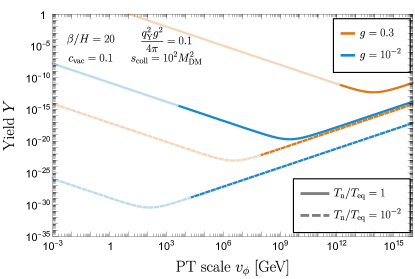
Figure 4: Yield of secondary particles $Y$ produced from collision of radiated reflected $U(1)$ gauge bosons $V$. Lines become lighter when free streaming conditions are not respected, and thus our derivation of the yield should be changed.

The discussion above applies to any bubbletron, including those where different populations are colliding. For concreteness, we now specify it to the case of a gauged $U(1)$, with $i=j=V$, for which [69]

$$P_{b\to V}\simeq\frac{g_{\rm emit}}{g_{b}}\frac{g^{2}}{16\pi^{2}}\log_{V}^{2},\quad\log_{V}^{2}=\log{\frac{m_{V}^{2}}{\mu^{2}}}\Big{(}\log{\frac{m_{V}^{2}}{\mu^{2}}}-2\Big{)},$$ (9)

where $g_{b}$ is the number of relativistic degrees of freedom in the bath and $g_{\rm emit}$ is the subset charged under $U(1)$, which can thus emit a $V$. For reference, in our figures we use $g_{\rm emit}=g_{\rm eff}=10$ and $g_{b}=106.75+g_{\rm emit}$. Here $\mu$ is an IR cut-off which, dealing with an abelian theory, we take as the thermal mass $\mu^{2}\simeq\frac{g_{\rm emit}}{10}g^{2}T_{n}^{2}$. In principle one should also include the screening length due to the high density of particles in the shell (see e.g. [39]), but the $V$’s are $U(1)$ singlets and so do not contribute at this order, and the density of fermions or scalars in the shell is suppressed, with respect to $n_{V}$, by extra powers of $g^{2}$ or $1/\gamma_{{\rm coll}}$. We assume further that a heavier fermion $Y$ with charge $q_{Y}$ under the $U(1)$ exists in the spectrum. We compute the $Y\bar{Y}$ production cross section as

$$\sigma_{VV\to Y\bar{Y}}=\dfrac{q_{Y}^{4}g^{4}}{4\pi s}\,f_{Y\bar{Y}}\xrightarrow[s\gg M_{Y}^{2}]{}\frac{q_{Y}^{4}g^{4}}{4\pi s}\Big{(}\log\frac{s}{M_{Y}^{2}}-1\Big{)}\,,$$ (10)

where in figures and numerical results we use the full expression $f_{Y\bar{Y}}(y\equiv\frac{4m_{Y}^{2}}{s})=(-\sqrt{1-y}(1+y)+(2+(2-y)y)\tanh^{-1}(\sqrt{1-y}))$. Using Eq. (3), $m_{V}=gv_{\phi}$, $n_{b}=g_{b}\zeta(3)T_{n}^{3}/\pi^{2}$ and $s_{\rm RH}=g_{\rm RH}2\pi^{2}T^{3}_{\rm RH}/45$, with $T_{\rm RH}=(30c_{{\rm vac}}/(g_{\rm RH}\pi^{2}))^{\frac{1}{4}}v_{\phi}$ the reheating temperature and $g_{\rm RH}$ the number of relativistic degrees of freedom after the PT, we find

$$Y_{Y+\bar{Y}}^{U(1)}\simeq 3.1\cdot 10^{-20}g^{2}\Big{(}\frac{T_{n}}{T_{\rm eq}}\Big{)}^{\!4}\Big{(}\frac{\gamma_{\rm run}}{\gamma_{{\rm coll}}}\Big{)}^{\!2}\frac{v_{\phi}}{\rm TeV}\frac{\beta/H}{20}\frac{g_{\rm emit}^{2}}{g_{b}}\Big{(}\frac{q_{Y}^{2}g^{2}/4\pi}{0.1}\Big{)}^{2}\Big{(}\frac{c_{{\rm vac}}}{0.1}\Big{)}^{\!\frac{3}{4}}\Big{(}\frac{100}{g_{\rm RH}}\Big{)}^{\!\frac{1}{4}}\frac{f_{Y\bar{Y}}\log_{V}^{4}}{100}\,.$$ (11)

$Y_{Y+\bar{Y}}^{U(1)}$ is visualized in Fig. 4 for some representative values of the parameters. We stress that Eqs. (11), and the more general one (8), apply only in regions of parameter space where the free-streaming conditions (see Fig. 3) are satisfied. We display this in Fig. 4 by interrupting the lines of $Y_{Y}^{U(1)}$ as soon as the free-streaming conditions are violated. Our calculations have potentially wide applications, whcih we begin to explore here for the production of heavy dark matter.

V Heavy dark matter

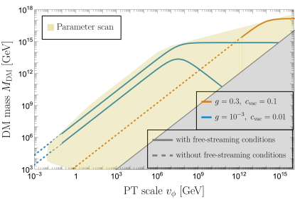
Figure 5: Mass of dark matter produced by a bubbletron of reflected $U(1)$ gauge bosons. Lines: $M_{\rm DM}$ in two representative scenarios, both with $\beta/H=20$ and $T_{n}=T_{\rm eq}$. Lines turn dashed when they stop satisfying the condition of shells free streaming. The champagne shaded area is the envelope of all the solid lines we obtain upon varying $g$, $T_{n}/T_{\rm eq}$, $\beta/H$, $c_{{\rm vac}}$, $q_{Y}$. See text for more details.

We now specify our discussion to the case where $Y$ is stable on cosmological scales, and thus a potential DM candidate. We assume zero initial abundance of $Y,\bar{Y}$ and impose that their yield from shell collisions reproduces the observed DM one, i.e. $Y_{Y+\bar{Y}}^{U(1)}=Y_{\rm Planck}^{\rm DM}\simeq 0.43\leavevmode\nobreak\ {\rm eV}/M_{\rm DM}$ [85] with $M_{Y}=M_{\rm DM}$. This allows us to plot lines of DM abundance on an $M_{\rm DM}-v_{\phi}$ plane, for any value of the other parameters $g$, $T_{n}$, etc. We do so varying the parameters as $1\geq T_{n}/T_{\rm eq}\geq 10^{-4}$, $1\geq g\geq 10^{-5}$, $10^{4}\geq\beta/H\geq 10$, $1\geq c_{{\rm vac}}\geq 10^{-3}$, $10^{-4}<g^{2}q_{Y}^{2}/4\pi<0.1$, with the perturbativity condition $P_{b\to V}<1$. We then discard all lines of DM abundance that do not satisfy the free streaming conditions visualized in Fig 3. The envelope of the remaining lines gives the maximal DM mass as a function of $v_{\phi}$, which we visualize in Fig. 5. For easiness of the reader, we also visualize the lines corresponding to two benchmark values of the parameters. One sees that in general there are two solutions that reproduce $Y_{\rm Planck}^{\rm DM}$, one for $M^{2}_{\rm DM}\to s_{\rm coll}/4$ and one for smaller $M_{\rm DM}$. At large $g$ the latter line falls in the region $M_{\rm DM}<v_{\phi}$. At large $v_{\phi}$, $\gamma_{{\rm coll}}=\gamma_{\rm run}$, which decreases because bubbles have less room to expand and $M_{\rm DM}$ saturates to a constant. We stop the plots at $v_{\phi}=10^{16}$ GeV in order to avoid the ‘ping-pong’ regime (see e.g. [39]) where gauge bosons are reflected multiple times. At small values of $v_{\phi}$ the free-streaming conditions impose small values of $g$.

VI Gravity waves from the phase transition

We finally compute the GW spectrum generated by the PT for ultra-relativistic bubble walls, which is an essential condition for the occurrence of the bubbletron scenario. According to whether their Lorentz factor $\gamma_{\rm coll}$ is set by $\gamma_{\rm run}$ or $\gamma_{{\rm LL}}$ in Eq. (3), the latent heat fraction $\alpha\equiv\Delta V/\rho_{\rm rad}|_{T_{n}}=\left(T_{\rm eq}/T_{n}\right)^{4}$ of the PT is either kept in the bubble wall kinetic energy or is transferred to the plasma in the form of ultra-relativistic shocks. In the former case, the GW spectrum is given by the bulk flow model [63], which has been calculated analytically [63] and numerically [64, 66, 86, 87]. It extends the envelop approximation [59, 61] by accounting for the propagation of bubble wall remnants long after the collision. In the latter case, ultra-relativistic shocks can be described by extremely thin and long-lived shells of stress-energy tensor [88]. From a gravitational point of view, they should be indistinguishable from stress-energy profile stored in the scalar field. Hence, the bulk flow model should offer a good description of the GW spectrum (also see [86]). First results in the moderately-relativistic regime $\gamma_{\rm coll}\lesssim 10$ support this choice [89]. We take the GW spectrum $\Omega_{\rm GW}h^{2}$ from [64] to which we impose a scaling in frequency $f^{3}$ for $f\lesssim H/2\pi$ as required by causality [90, 91, 92, 93]. In Fig. 6 we display $\Omega_{\rm GW}h^{2}$ for three different benchmark points, the one for $v_{\phi}=0.1$ GeV can provide a good fit [94, 95] of pulsar timing array data [96, 97, 98, 99].

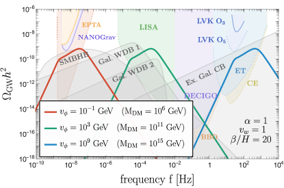
Figure 6: Lines: GW signal from a $U(1)$ gauge phase transition. The associated bubbletron can produce dark matter with mass $M_{\rm DM}$ up to the values written in the figure for each $v_{\phi}$, for $\beta/H=20$ and $\alpha\equiv(\frac{T_{n}}{T_{\rm eq}})^{4}=1$. Shaded in gray: expected foregrounds [100, 101, 102, 103, 104, 105]. Shaded in color: current [105, 106, 107] and projected limits [108, 109, 110, 111, 112, 113].

VII Discussion and Outlook

In this letter we have pointed out the existence of ‘bubbletrons’, i.e. particle accelerators and colliders in the early universe that are generically realised by first-order phase transitions with ultrarelativistic bubble walls. Among many processes that lead to bubbletrons, we have focused on radiated reflected particles at the walls in gauge PTs and computed their scattering energies (see Fig. 2) if they free-stream until collision (see [82] and Fig. 3). These collision can produce particles much heavier than the scale $v_{\phi}$ of the PT and of inflation, with sizeable yields displayed in Fig. 4. We stress that bubbletrons are predicted in any PT with fast bubble walls, so they do not necessarily require supercooling (i.e. $T_{n}<T_{\rm eq}$). As an application, we found that they can produce DM as heavy as the PeV (grand-unification) scale for $v_{\phi}\gtrsim 10^{-2}(10^{8})$ GeV, see Fig. 5.

Our study realises a new connection between primordial GW signals and physics at energy scales otherwise unaccessible not only in the laboratory but, so far, also in the early universe. In the example of heavy DM, these GW could be accompanied by high energy cosmic rays from decays of DM, if unstable: this could intriguingly link, e.g., GW at pulsar timing arrays with high-energy neutrinos and photons at IceCube, KM3NeT, CTA or LHAASO.

Our study opens several avenues of exploration. These include bubbletrons other than those induced by radiated reflected particles, or in the region where shells do not free-stream, and applications for baryogenesis and possible trans-Planckian scatterings in the early universe. We plan to return to some of these aspects in future work.

Acknowledgements.—YG is grateful to the Azrieli Foundation for the award of an Azrieli Fellowship. This work was supported by the European Union’s Horizon 2020 research and innovation programme under grant agreement No 101002846, ERC CoG “CosmoChart.”

References

- Kajantie et al. [1996] K. Kajantie, M. Laine, K. Rummukainen, and M. E. Shaposhnikov, Is there a hot electroweak phase transition at ?, Phys. Rev. Lett. 77, 2887 (1996), arXiv:hep-ph/9605288 .
- Aoki et al. [2006] Y. Aoki, G. Endrodi, Z. Fodor, S. D. Katz, and K. K. Szabo, The Order of the quantum chromodynamics transition predicted by the standard model of particle physics, Nature 443, 675 (2006), arXiv:hep-lat/0611014 .
- Creminelli et al. [2002] P. Creminelli, A. Nicolis, and R. Rattazzi, Holography and the electroweak phase transition, JHEP 03, 051, arXiv:hep-th/0107141 [hep-th] .
- Nardini et al. [2007] G. Nardini, M. Quiros, and A. Wulzer, A Confining Strong First-Order Electroweak Phase Transition, JHEP 09, 077, arXiv:0706.3388 [hep-ph] .
- Konstandin and Servant [2011] T. Konstandin and G. Servant, Cosmological Consequences of Nearly Conformal Dynamics at the TeV scale, JCAP 1112, 009, arXiv:1104.4791 [hep-ph] .
- Craig et al. [2020] N. Craig, N. Levi, A. Mariotti, and D. Redigolo, Ripples in Spacetime from Broken Supersymmetry, JHEP 21, 184, arXiv:2011.13949 [hep-ph] .
- Delle Rose et al. [2020] L. Delle Rose, G. Panico, M. Redi, and A. Tesi, Gravitational Waves from Supercool Axions, JHEP 04, 025, arXiv:1912.06139 [hep-ph] .
- Von Harling et al. [2020] B. Von Harling, A. Pomarol, O. Pujolàs, and F. Rompineve, Peccei-Quinn Phase Transition at LIGO, JHEP 04, 195, arXiv:1912.07587 [hep-ph] .
- Greljo et al. [2020] A. Greljo, T. Opferkuch, and B. A. Stefanek, Gravitational Imprints of Flavor Hierarchies, Phys. Rev. Lett. 124, 171802 (2020), arXiv:1910.02014 [hep-ph] .
- Jinno and Takimoto [2017] R. Jinno and M. Takimoto, Probing a classically conformal B-L model with gravitational waves, Phys. Rev. D 95, 015020 (2017), arXiv:1604.05035 [hep-ph] .
- Hawking et al. [1982] S. W. Hawking, I. G. Moss, and J. M. Stewart, Bubble Collisions in the Very Early Universe, Phys. Rev. D26, 2681 (1982).
- Kodama et al. [1982] H. Kodama, M. Sasaki, and K. Sato, Abundance of Primordial Holes Produced by Cosmological First Order Phase Transition, Prog. Theor. Phys. 68, 1979 (1982).
- Khlopov et al. [1998] M. Y. Khlopov, R. V. Konoplich, S. G. Rubin, and A. S. Sakharov, Formation of Black Holes in First Order Phase Transitions, (1998), arXiv:hep-ph/9807343 .
- Lewicki and Vaskonen [2020a] M. Lewicki and V. Vaskonen, On bubble collisions in strongly supercooled phase transitions, Phys. Dark Univ. 30, 100672 (2020a), arXiv:1912.00997 [astro-ph.CO] .
- Gross et al. [2021] C. Gross, G. Landini, A. Strumia, and D. Teresi, Dark Matter as dark dwarfs and other macroscopic objects: multiverse relics?, JHEP 09, 033, arXiv:2105.02840 [hep-ph] .
- Liu et al. [2022] J. Liu, L. Bian, R.-G. Cai, Z.-K. Guo, and S.-J. Wang, Primordial Black Hole Production during First-Order Phase Transitions, Phys. Rev. D 105, L021303 (2022), arXiv:2106.05637 [astro-ph.CO] .
- Jung and Okui [2021] T. H. Jung and T. Okui, Primordial Black Holes from Bubble Collisions during a First-Order Phase Transition, (2021), arXiv:2110.04271 [hep-ph] .
- Hashino et al. [2021] K. Hashino, S. Kanemura, and T. Takahashi, Primordial Black Holes as a Probe of Strongly First-Order Electroweak Phase Transition, (2021), arXiv:2111.13099 [hep-ph] .
- Hashino et al. [2022] K. Hashino, S. Kanemura, T. Takahashi, and M. Tanaka, Probing First-Order Electroweak Phase Transition via Primordial Black Holes in the Effective Field Theory, (2022), arXiv:2211.16225 [hep-ph] .
- Lewicki et al. [2023] M. Lewicki, P. Toczek, and V. Vaskonen, Primordial black holes from strong first-order phase transitions, (2023), arXiv:2305.04924 [astro-ph.CO] .
- Gouttenoire and Volansky [2023] Y. Gouttenoire and T. Volansky, Primordial Black Holes from Supercooled Phase Transitions, (2023), arXiv:2305.04942 [hep-ph] .
- Aharonov and Bohm [1959] Y. Aharonov and D. Bohm, Significance of Electromagnetic Potentials in the Quantum Theory, Phys. Rev. 115, 485 (1959).
- Nielsen and Olesen [1973] H. B. Nielsen and P. Olesen, Vortex Line Models for Dual Strings, Nucl. Phys. B 61, 45 (1973).
- Kibble [1976] T. W. B. Kibble, Topology of Cosmic Domains and Strings, J. Phys. A 9, 1387 (1976).
- Gouttenoire et al. [2020a] Y. Gouttenoire, G. Servant, and P. Simakachorn, Beyond the Standard Models with Cosmic Strings, JCAP 07, 032, arXiv:1912.02569 [hep-ph] .
- Gouttenoire et al. [2020b] Y. Gouttenoire, G. Servant, and P. Simakachorn, BSM with Cosmic Strings: Heavy, up to EeV mass, Unstable Particles, JCAP 07, 016, arXiv:1912.03245 [hep-ph] .
- Hogan [1983] C. J. Hogan, Magnetohydrodynamic Effects of a First-Order Cosmological Phase Transition, Phys. Rev. Lett. 51, 1488 (1983).
- Quashnock et al. [1989] J. M. Quashnock, A. Loeb, and D. N. Spergel, Magnetic Field Generation during the Cosmological QCD Phase Transition, Astrophys. J. Lett. 344, L49 (1989).
- Vachaspati [1991] T. Vachaspati, Magnetic Fields from Cosmological Phase Transitions, Phys. Lett. B 265, 258 (1991).
- Enqvist and Olesen [1993] K. Enqvist and P. Olesen, On Primordial Magnetic Fields of Electroweak Origin, Phys. Lett. B 319, 178 (1993), arXiv:hep-ph/9308270 .
- Sigl et al. [1997] G. Sigl, A. V. Olinto, and K. Jedamzik, Primordial Magnetic Fields from Cosmological First Order Phase Transitions, Phys. Rev. D 55, 4582 (1997), arXiv:astro-ph/9610201 .
- Ahonen and Enqvist [1998] J. Ahonen and K. Enqvist, Magnetic Field Generation in First Order Phase Transition Bubble Collisions, Phys. Rev. D 57, 664 (1998), arXiv:hep-ph/9704334 .
- Ellis et al. [2020] J. Ellis, M. Lewicki, and V. Vaskonen, Updated Predictions for Gravitational Waves Produced in a Strongly Supercooled Phase Transition, JCAP 11, 020, arXiv:2007.15586 [astro-ph.CO] .
- Falkowski and No [2013] A. Falkowski and J. M. No, Non-thermal Dark Matter Production from the Electroweak Phase Transition: Multi-TeV WIMPs and ’Baby-Zillas’, JHEP 02, 034, arXiv:1211.5615 [hep-ph] .
- Hambye et al. [2018] T. Hambye, A. Strumia, and D. Teresi, Super-cool Dark Matter, JHEP 08, 188, arXiv:1805.01473 [hep-ph] .
- Baldes and Garcia-Cely [2019] I. Baldes and C. Garcia-Cely, Strong gravitational radiation from a simple dark matter model, JHEP 05, 190, arXiv:1809.01198 [hep-ph] .
- Baker et al. [2019] M. J. Baker, J. Kopp, and A. J. Long, Filtered Dark Matter at a First Order Phase Transition, (2019), arXiv:1912.02830 [hep-ph] .
- Chway et al. [2020] D. Chway, T. H. Jung, and C. S. Shin, Dark matter filtering-out effect during a first-order phase transition, Phys. Rev. D 101, 095019 (2020), arXiv:1912.04238 [hep-ph] .
- Baldes et al. [2021a] I. Baldes, Y. Gouttenoire, and F. Sala, String Fragmentation in Supercooled Confinement and Implications for Dark Matter, JHEP 04, 278, arXiv:2007.08440 [hep-ph] .
- Azatov et al. [2021a] A. Azatov, M. Vanvlasselaer, and W. Yin, Dark Matter production from relativistic bubble walls, JHEP 03, 288, arXiv:2101.05721 [hep-ph] .
- Baldes et al. [2022] I. Baldes, Y. Gouttenoire, F. Sala, and G. Servant, Supercool composite Dark Matter beyond 100 TeV, JHEP 07, 084, arXiv:2110.13926 [hep-ph] .
- Kierkla et al. [2022] M. Kierkla, A. Karam, and B. Swiezewska, Conformal Model for Gravitational Waves and Dark Matter: a Status Update, (2022), arXiv:2210.07075 [astro-ph.CO] .
- Freese and Winkler [2023] K. Freese and M. W. Winkler, Dark matter and gravitational waves from a dark big bang, Phys. Rev. D 107, 083522 (2023), arXiv:2302.11579 [astro-ph.CO] .
- Kuzmin et al. [1985] V. A. Kuzmin, V. A. Rubakov, and M. E. Shaposhnikov, On the Anomalous Electroweak Baryon Number Nonconservation in the Early Universe, Phys. Lett. B 155, 36 (1985).
- Shaposhnikov [1986] M. E. Shaposhnikov, Possible Appearance of the Baryon Asymmetry of the Universe in an Electroweak Theory, JETP Lett. 44, 465 (1986).
- Cohen et al. [1990] A. G. Cohen, D. B. Kaplan, and A. E. Nelson, Weak Scale Baryogenesis, Phys. Lett. B 245, 561 (1990).
- Shaposhnikov [1992] M. E. Shaposhnikov, Standard Model Solution of the Baryogenesis Problem, Phys. Lett. B 277, 324 (1992), [Erratum: Phys.Lett.B 282, 483 (1992)].
- Farrar and Shaposhnikov [1993] G. R. Farrar and M. E. Shaposhnikov, Baryon Asymmetry of the Universe in the Minimal Standard Model, Phys. Rev. Lett. 70, 2833 (1993), [Erratum: Phys.Rev.Lett. 71, 210 (1993)], arXiv:hep-ph/9305274 .
- Huet and Sather [1995] P. Huet and E. Sather, Electroweak Baryogenesis and Standard Model CP Violation, Phys. Rev. D 51, 379 (1995), arXiv:hep-ph/9404302 .
- Gavela et al. [1994] M. B. Gavela, P. Hernandez, J. Orloff, O. Pene, and C. Quimbay, Standard Model CP Violation and Baryon Asymmetry. Part 2: Finite Temperature, Nucl. Phys. B 430, 382 (1994), arXiv:hep-ph/9406289 .
- Morrissey and Ramsey-Musolf [2012] D. E. Morrissey and M. J. Ramsey-Musolf, Electroweak Baryogenesis, New J. Phys. 14, 125003 (2012), arXiv:1206.2942 [hep-ph] .
- Konstandin [2013] T. Konstandin, Quantum Transport and Electroweak Baryogenesis, Phys. Usp. 56, 747 (2013), arXiv:1302.6713 [hep-ph] .
- Servant [2018] G. Servant, The serendipity of electroweak baryogenesis, Phil. Trans. Roy. Soc. Lond. A 376, 20170124 (2018), arXiv:1807.11507 [hep-ph] .
- Katz and Riotto [2016] A. Katz and A. Riotto, Baryogenesis and Gravitational Waves from Runaway Bubble Collisions, JCAP 1611 (11), 011, arXiv:1608.00583 [hep-ph] .
- Azatov et al. [2021b] A. Azatov, M. Vanvlasselaer, and W. Yin, Baryogenesis via Relativistic Bubble Walls, JHEP 10, 043, arXiv:2106.14913 [hep-ph] .
- Baldes et al. [2021b] I. Baldes, S. Blasi, A. Mariotti, A. Sevrin, and K. Turbang, Baryogenesis via relativistic bubble expansion, Phys. Rev. D 104, 115029 (2021b), arXiv:2106.15602 [hep-ph] .
- Witten [1984] E. Witten, Cosmic Separation of Phases, Phys. Rev. D30, 272 (1984).
- Kosowsky et al. [1992] A. Kosowsky, M. S. Turner, and R. Watkins, Gravitational Waves from First Order Cosmological Phase Transitions, Phys. Rev. Lett. 69, 2026 (1992).
- Kamionkowski et al. [1994] M. Kamionkowski, A. Kosowsky, and M. S. Turner, Gravitational radiation from first order phase transitions, Phys. Rev. D49, 2837 (1994), arXiv:astro-ph/9310044 [astro-ph] .
- Randall and Servant [2007] L. Randall and G. Servant, Gravitational waves from warped spacetime, JHEP 05, 054, arXiv:hep-ph/0607158 [hep-ph] .
- Huber and Konstandin [2008] S. J. Huber and T. Konstandin, Gravitational Wave Production by Collisions: More Bubbles, JCAP 0809, 022, arXiv:0806.1828 [hep-ph] .
- Hindmarsh et al. [2014] M. Hindmarsh, S. J. Huber, K. Rummukainen, and D. J. Weir, Gravitational waves from the sound of a first order phase transition, Phys. Rev. Lett. 112, 041301 (2014), arXiv:1304.2433 [hep-ph] .
- Jinno and Takimoto [2019] R. Jinno and M. Takimoto, Gravitational waves from bubble dynamics: Beyond the Envelope, JCAP 1901, 060, arXiv:1707.03111 [hep-ph] .
- Konstandin [2018] T. Konstandin, Gravitational radiation from a bulk flow model, JCAP 1803 (03), 047, arXiv:1712.06869 [astro-ph.CO] .
- Cutting et al. [2018] D. Cutting, M. Hindmarsh, and D. J. Weir, Gravitational waves from vacuum first-order phase transitions: from the envelope to the lattice, Phys. Rev. D97, 123513 (2018), arXiv:1802.05712 [astro-ph.CO] .
- Lewicki and Vaskonen [2020b] M. Lewicki and V. Vaskonen, Gravitational wave spectra from strongly supercooled phase transitions, (2020b), arXiv:2007.04967 [astro-ph.CO] .
- Hindmarsh et al. [2021] M. B. Hindmarsh, M. Lüben, J. Lumma, and M. Pauly, Phase transitions in the early universe, SciPost Phys. Lect. Notes 24, 1 (2021), arXiv:2008.09136 [astro-ph.CO] .
- Gouttenoire [2022] Y. Gouttenoire, Beyond the Standard Model Cocktail, (2022), arXiv:2207.01633 [hep-ph] .
- Gouttenoire et al. [2022] Y. Gouttenoire, R. Jinno, and F. Sala, Friction pressure on relativistic bubble walls, JHEP 05, 004, arXiv:2112.07686 [hep-ph] .
- Baldes et al. [2023] I. Baldes, Y. Gouttenoire, and F. Sala, Hot and heavy dark matter from a weak scale phase transition, SciPost Phys. 14, 033 (2023), arXiv:2207.05096 [hep-ph] .
- Garcia Garcia et al. [2022] I. Garcia Garcia, G. Koszegi, and R. Petrossian-Byrne, Reflections on Bubble Walls, (2022), arXiv:2212.10572 [hep-ph] .
- Arkani-Hamed and Maldacena [2015] N. Arkani-Hamed and J. Maldacena, Cosmological Collider Physics, (2015), arXiv:1503.08043 [hep-th] .
- Enqvist et al. [1992] K. Enqvist, J. Ignatius, K. Kajantie, and K. Rummukainen, Nucleation and bubble growth in a first order cosmological electroweak phase transition, Phys. Rev. D45, 3415 (1992).
- Konstandin and No [2011] T. Konstandin and J. M. No, Hydrodynamic obstruction to bubble expansion, JCAP 02, 008, arXiv:1011.3735 [hep-ph] .
- Cline et al. [2021] J. M. Cline, A. Friedlander, D.-M. He, K. Kainulainen, B. Laurent, and D. Tucker-Smith, Baryogenesis and gravity waves from a UV-completed electroweak phase transition, Phys. Rev. D 103, 123529 (2021), arXiv:2102.12490 [hep-ph] .
- Laurent and Cline [2022] B. Laurent and J. M. Cline, First principles determination of bubble wall velocity, Phys. Rev. D 106, 023501 (2022), arXiv:2204.13120 [hep-ph] .
- De Curtis et al. [2023] S. De Curtis, L. Delle Rose, A. Guiggiani, A. Gil Muyor, and G. Panico, Collision integrals for cosmological phase transitions, JHEP 05, 194, arXiv:2303.05846 [hep-ph] .
- Bodeker and Moore [2009] D. Bodeker and G. D. Moore, Can electroweak bubble walls run away?, JCAP 0905, 009, arXiv:0903.4099 [hep-ph] .
- Azatov and Vanvlasselaer [2021] A. Azatov and M. Vanvlasselaer, Bubble wall velocity: heavy physics effects, JCAP 01, 058, arXiv:2010.02590 [hep-ph] .
- Bodeker and Moore [2017] D. Bodeker and G. D. Moore, Electroweak Bubble Wall Speed Limit, JCAP 1705 (05), 025, arXiv:1703.08215 [hep-ph] .
- [81] Y. Gouttenoire and et al., Wall decay during first-order phase transition, In progress .
- [82] I. Baldes, M. Dichtl, Y. Gouttenoire, and F. Sala, (To Appear), arXiv:23mm.nnnnn .
- Croon et al. [2019] D. Croon, T. E. Gonzalo, L. Graf, N. Košnik, and G. White, GUT Physics in the era of the LHC, Front. in Phys. 7, 76 (2019), arXiv:1903.04977 [hep-ph] .
- Akrami et al. [2020] Y. Akrami et al. (Planck), Planck 2018 results. X. Constraints on inflation, Astron. Astrophys. 641, A10 (2020), arXiv:1807.06211 [astro-ph.CO] .
- Aghanim et al. [2020] N. Aghanim et al. (Planck), Planck 2018 results. VI. Cosmological parameters, Astron. Astrophys. 641, A6 (2020), [Erratum: Astron.Astrophys. 652, C4 (2021)], arXiv:1807.06209 [astro-ph.CO] .
- Lewicki and Vaskonen [2021] M. Lewicki and V. Vaskonen, Gravitational waves from colliding vacuum bubbles in gauge theories, Eur. Phys. J. C 81, 437 (2021), [Erratum: Eur.Phys.J.C 81, 1077 (2021)], arXiv:2012.07826 [astro-ph.CO] .
- Cutting et al. [2020] D. Cutting, E. G. Escartin, M. Hindmarsh, and D. J. Weir, Gravitational waves from vacuum first order phase transitions II: from thin to thick walls, (2020), arXiv:2005.13537 [astro-ph.CO] .
- Jinno et al. [2019] R. Jinno, H. Seong, M. Takimoto, and C. M. Um, Gravitational waves from first-order phase transitions: Ultra-supercooled transitions and the fate of relativistic shocks, JCAP 10, 033, arXiv:1905.00899 [astro-ph.CO] .
- Jinno et al. [2022] R. Jinno, B. Shakya, and J. van de Vis, Gravitational Waves from Feebly Interacting Particles in a First Order Phase Transition, (2022), arXiv:2211.06405 [gr-qc] .
- Durrer and Caprini [2003] R. Durrer and C. Caprini, Primordial Magnetic Fields and Causality, JCAP 11, 010, arXiv:astro-ph/0305059 .
- Caprini et al. [2009] C. Caprini, R. Durrer, T. Konstandin, and G. Servant, General Properties of the Gravitational Wave Spectrum from Phase Transitions, Phys. Rev. D79, 083519 (2009), arXiv:0901.1661 [astro-ph.CO] .
- Cai et al. [2020] R.-G. Cai, S. Pi, and M. Sasaki, Universal Infrared Scaling of Gravitational Wave Background Spectra, Phys. Rev. D 102, 083528 (2020), arXiv:1909.13728 [astro-ph.CO] .
- Hook et al. [2021] A. Hook, G. Marques-Tavares, and D. Racco, Causal Gravitational Waves as a Probe of Free Streaming Particles and the Expansion of the Universe, JHEP 02, 117, arXiv:2010.03568 [hep-ph] .
- Arzoumanian et al. [2021] Z. Arzoumanian et al. (NANOGrav), Searching for Gravitational Waves from Cosmological Phase Transitions with the NANOGrav 12.5-Year Dataset, Phys. Rev. Lett. 127, 251302 (2021), arXiv:2104.13930 [astro-ph.CO] .
- Bringmann et al. [2023] T. Bringmann, P. F. Depta, T. Konstandin, K. Schmidt-Hoberg, and C. Tasillo, Does NANOGrav observe a dark sector phase transition?, (2023), arXiv:2306.09411 [astro-ph.CO] .
- Arzoumanian et al. [2020] Z. Arzoumanian et al. (NANOGrav), The Nanograv 12.5 Yr Data Set: Search for an Isotropic Stochastic Gravitational-Wave Background, Astrophys. J. Lett. 905, L34 (2020), arXiv:2009.04496 [astro-ph.HE] .
- Goncharov et al. [2021] B. Goncharov et al., On the Evidence for a Common-spectrum Process in the Search for the Nanohertz Gravitational-wave Background with the Parkes Pulsar Timing Array, Astrophys. J. Lett. 917, L19 (2021), arXiv:2107.12112 [astro-ph.HE] .
- Chen et al. [2021] S. Chen et al., Common-red-signal analysis with 24-yr high-precision timing of the European Pulsar Timing Array: inferences in the stochastic gravitational-wave background search, Mon. Not. Roy. Astron. Soc. 508, 4970 (2021), arXiv:2110.13184 [astro-ph.HE] .
- Antoniadis et al. [2022] J. Antoniadis et al., The International Pulsar Timing Array second data release: Search for an isotropic gravitational wave background, Mon. Not. Roy. Astron. Soc. 510, 4873 (2022), arXiv:2201.03980 [astro-ph.HE] .
- Rosado [2011] P. A. Rosado, Gravitational wave background from binary systems, Phys. Rev. D 84, 084004 (2011), arXiv:1106.5795 [gr-qc] .
- Lamberts et al. [2019] A. Lamberts, S. Blunt, T. B. Littenberg, S. Garrison-Kimmel, T. Kupfer, and R. E. Sanderson, Predicting the Lisa White Dwarf Binary Population in the Milky Way with Cosmological Simulations, Mon. Not. Roy. Astron. Soc. 490, 5888 (2019), arXiv:1907.00014 [astro-ph.HE] .
- Boileau et al. [2022] G. Boileau, A. C. Jenkins, M. Sakellariadou, R. Meyer, and N. Christensen, Ability of Lisa to Detect a Gravitational-Wave Background of Cosmological Origin: the Cosmic String Case, Phys. Rev. D 105, 023510 (2022), arXiv:2109.06552 [gr-qc] .
- Boileau et al. [2023] G. Boileau, N. Christensen, C. Gowling, M. Hindmarsh, and R. Meyer, Prospects for LISA to detect a gravitational-wave background from first order phase transitions, JCAP 02, 056, arXiv:2209.13277 [gr-qc] .
- Robson et al. [2019] T. Robson, N. J. Cornish, and C. Liu, The Construction and Use of Lisa Sensitivity Curves, Class. Quant. Grav. 36, 105011 (2019), arXiv:1803.01944 [astro-ph.HE] .
- Abbott et al. [2021] R. Abbott et al. (KAGRA, Virgo, LIGO Scientific), Upper limits on the isotropic gravitational-wave background from Advanced LIGO and Advanced Virgo’s third observing run, Phys. Rev. D 104, 022004 (2021), arXiv:2101.12130 [gr-qc] .
- Lentati et al. [2015] L. Lentati et al., European Pulsar Timing Array Limits On An Isotropic Stochastic Gravitational-Wave Background, Mon. Not. Roy. Astron. Soc. 453, 2576 (2015), arXiv:1504.03692 [astro-ph.CO] .
- Arzoumanian et al. [2018] Z. Arzoumanian et al. (NANOGRAV), The NANOGrav 11-year Data Set: Pulsar-timing Constraints On The Stochastic Gravitational-wave Background, Astrophys. J. 859, 47 (2018), arXiv:1801.02617 [astro-ph.HE] .
- Audley et al. [2017] H. Audley et al. (LISA), Laser Interferometer Space Antenna, (2017), arXiv:1702.00786 [astro-ph.IM] .
- Yagi and Seto [2011] K. Yagi and N. Seto, Detector Configuration of Decigo/Bbo and Identification of Cosmological Neutron-Star Binaries, Phys. Rev. D 83, 044011 (2011), [Erratum: Phys.Rev.D 95, 109901 (2017)], arXiv:1101.3940 [astro-ph.CO] .
- Hild et al. [2011] S. Hild et al., Sensitivity Studies for Third-Generation Gravitational Wave Observatories, Class. Quant. Grav. 28, 094013 (2011), arXiv:1012.0908 [gr-qc] .
- Punturo et al. [2010] M. Punturo et al., The Einstein Telescope: A third-generation gravitational wave observatory, Proceedings, 14th Workshop on Gravitational wave data analysis (GWDAW-14): Rome, Italy, January 26-29, 2010, Class. Quant. Grav. 27, 194002 (2010).
- Abbott et al. [2018] B. P. Abbott et al. (KAGRA, LIGO Scientific, Virgo, VIRGO), Prospects for observing and localizing gravitational-wave transients with Advanced LIGO, Advanced Virgo and KAGRA, Living Rev. Rel. 21, 3 (2018), arXiv:1304.0670 [gr-qc] .
- Janssen et al. [2015] G. Janssen et al., Gravitational wave astronomy with the SKA, PoS AASKA14, 037 (2015), arXiv:1501.00127 [astro-ph.IM] .