Tommaso Salvatori^1,4     Luca Pinchetti²     Amine M’Charrak²
Beren Millidge³     Thomas Lukasiewicz^4,2
1 VERSES Research Lab, Los Angeles, CA 90016, USA
² Department of Computer Science, University of Oxford, UK
³ MRC Brain Network Dynamics Unit, University of Oxford, UK
⁴ Institute of Logic and Computation, TU Wien, Austria
Corresponding author: tommaso.salvatori@verses.ai.

Causal Inference via Predictive Coding

Tommaso Salvatori^1,4     Luca Pinchetti²     Amine M’Charrak²
Beren Millidge³     Thomas Lukasiewicz^4,2
1 VERSES Research Lab, Los Angeles, CA 90016, USA
² Department of Computer Science, University of Oxford, UK
³ MRC Brain Network Dynamics Unit, University of Oxford, UK
⁴ Institute of Logic and Computation, TU Wien, Austria
Corresponding author: tommaso.salvatori@verses.ai.

Abstract

Bayesian and causal inference are fundamental processes for intelligence. Bayesian inference models observations: what can be inferred about y if we observe a related variable x? Causal inference models interventions: if we directly change x, how will y change? Predictive coding is a neuroscience-inspired method for performing Bayesian inference on continuous state variables using local information only. In this work, we go beyond Bayesian inference, and show how a simple change in the inference process of predictive coding enables interventional and counterfactual inference in scenarios where the causal graph is known. We then extend our results, and show how predictive coding can be generalized to cases where this graph is unknown, and has to be inferred from data, hence performing causal discovery. What results is a novel and straightforward technique that allows us to perform end-to-end causal inference on predictive-coding-based structural causal models, and demonstrate its utility for potential applications in machine learning.

1 Introduction

Our brain is generally considered to be an inference machine, where a generative model of the world updates internal states to predict upcoming observations (Friston, 2012; Seth, 2014; Clark, 2013; Knill and Pouget, 2004). When observations from the external world do not match our internal predictions, this generates a prediction error, or surprise, necessitating correction. Handling this discrepancy involves the update of the internal states to better model their posterior distribution, given the observations. In variational inference, this is done by minimizing a quantity called the variational free energy. When our generative model is formed by a hierarchy of Gaussian distributions, the process of minimizing the variational free energy is equivalent to minimizing the prediction errors at the neuronal level, hence connecting the theories of variational inference and predictive coding (Friston, 2003, 2005, 2010, 2008; Rao and Ballard, 1999).

Conventional literature on predictive coding primarily deals with hierarchical generative models relating top-down predictions to internal states and external stimuli (Rao and Ballard, 1999; Friston, 2005, 2008; Whittington and Bogacz, 2017). While providing a good explanation of the general process, it fails to model networks with a more complex topology which can, in contrast, be modeled using Bayesian networks (i.e., directed acyclic graphical models) (Pearl, 1985). Recent work has shown that predictive coding can also perform learning on non-hierarchical structures (Salvatori et al., 2022a) such as Bayesian networks. To do so, we can consider every node of the Bayesian network to be an independent generative model, whose state is dependent on its own Markov blanket, the set of nodes that contain the information needed to compute its posterior distribution. In Bayesian networks, the Markov blanket of a node is the set of its parent nodes, its children nodes, and all the parents of the children nodes. This concept is illustrated in Fig. 1 (left).

Classical predictive coding approaches are limited to the computation of correlations (Rao and Ballard, 1999; Friston, 2005). This work extends previous research by demonstrating that predictive coding networks can accurately model causal relationships between the variables of a system, and naturally perform interventional and counterfactual inference. Research on causality is divided into two primary areas: causal inference, which aims to infer the effect of an intervention in a known system, and causal discovery, which aims to discover the causal graphical model underlying observational data (a dataset). Here, we tackle both tasks. We first show how predictive coding models, structured according to a known probabilistic graphical model, are able to naturally model interventions using a differentiable framework that aims to minimize a variational free energy (Friston, 2005; Rao and Ballard, 1999), with only a simple and slight adjustment to their standard Bayesian inference procedure. Next, we show how to use the same framework to perform structure learning, which is the problem of inferring causal dependencies from data (Heinze-Deml et al., 2018). We demonstrate that predictive coding models are able to perform end-to-end causal inference, which is the joint task of observing a dataset, learn a causal graph, and then using it to perform causal inference tasks. Our contributions are summarized as follows:

• In Section 2, we review the basic concepts of Bayesian networks, and their connection with causal inference. Then, we show how the predictive coding framework developed to train graphs with arbitrary graph topologies (Salvatori et al., 2022a) can be used to perform conditional inference on Bayesian networks.

• In Section 3, we show how to model interventions in predictive coding networks. This can be simply done by fixing the prediction error of a specific node to zero during the inference process. Empirically, we test our claims on predictive coding-based structural causal models, and show promising results on machine learning and causal inference benchmarks (De Brouwer, 2022).

• In Section 4, we show both theoretically and empirically how to use predictive coding graphs to perform causal structure learning from data. This shows that predictive coding is an end-to-end causality engine, able to answer causal queries without previous knowledge of the parent-child relationships.

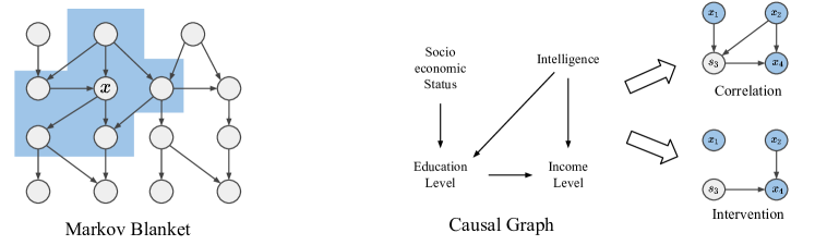
Figure 1: Left: An example of the Markov blanket of a node $\mathbf{x}$. Right: An example of a causal graph in society. The corresponding Bayesian network has the joint probability $p(\mathbf{x}_{1},\mathbf{x}_{2},\mathbf{x}_{3},\mathbf{x}_{4})=p(\mathbf{x}_{1})p(\mathbf{x}_{2})p(\mathbf{x}_{3}\mid\mathbf{x}_{1},\mathbf{x}_{2})p(\mathbf{x}_{4}\mid\mathbf{x}_{2},\mathbf{x}_{3})$. The arrows point on conditional and interventional inference on the same causal graph. In a conditional query, we know from data that $\mathbf{x}_{3}=\mathbf{s}_{3}$. The goal of an interventional query is to infer the effect that $\mathbf{s}_{3}$ causes, that is, compute the posterior $p(\mathbf{x}_{1},\mathbf{x}_{2},\mathbf{x}_{4}\mid\mathbf{x}_{3}=\mathbf{s}_{3})$ in the intervention graph. In an interventional query, we compute $p(\mathbf{x}_{4}\mid do(\mathbf{x}_{3}=\mathbf{s}_{3}))$. To do that, we have to first act on the structure of the graph, and then perform conditional inference on the new graph, with the joint probability $p(\mathbf{x}_{1},\mathbf{x}_{2},\mathbf{x}_{3},\mathbf{x}_{4})=p(\mathbf{x}_{1})p(\mathbf{x}_{2})p(\mathbf{x}_{4}\mid\mathbf{x}_{2},\mathbf{x}_{3})$.

2 Bayesian Networks and Predictive Coding

Assume that we have a set of $N$ random variables $\mathbf{X}=\{\mathbf{x}_{1},\dots,\mathbf{x}_{N}\}$, with $\mathbf{x}_{i}\in\mathbb{R}^{d}$. Relations among variables are represented by a directed graph $G=(V,E)$, also called causal graph of $S$. Every vertex $v_{i}\,{\in}\,V$ represents a random variable $\mathbf{x}_{i}$, and every edge $(i,j)$ represents a causal relation from $\mathbf{x}_{i}$ to $\mathbf{x}_{j}$. The causal graph defines the joint distribution of the system, computed as follows:

$$p(\mathbf{x}_{1},\dots,\mathbf{x}_{N})=\Pi_{i=1}^{N}\,p(\mathbf{x}_{i}|par(\mathbf{x}_{i})),$$

where $par(\mathbf{x}_{i})$ is the set of parent nodes of $\mathbf{x}_{i}$. An example of a causal graph is shown in Fig. 1. Given the values of some random variables, we want to infer the causes that generate them. Here, these causes correspond to the missing (and unconstrained) variables of the system. More formally, let us partition the set of variables $\mathbf{X}=\mathbf{X}_{data}\ \cup\ \mathbf{X}_{unk}$, where $\mathbf{X}_{data}=\mathbf{x}_{i_{1}},\dots,\mathbf{x}_{i_{n}}$ is a subset of variables of which we have information via a data point $\mathbf{S}_{data}=\mathbf{s}_{i_{1}},\dots,\mathbf{s}_{i_{n}}$. We want to infer the values of the unknown nodes. This is trivial when a data point $\mathbf{s}_{i}$ is the root of a tree only formed by unknown variables. In this case, in fact, it is possible to compute the unknown variables via a forward pass. The problem, however, becomes more complex, and often intractable, when it is necessary to infer missing nodes that are parents of data points, as we need to invert the generative model of specific nodes. When dealing with continuous variables, we can use predictive coding to perform such an inversion (Friston, 2005).

Posterior distribution.

In most cases, the computation of the posterior distribution $p(\mathbf{X}_{unk}|\mathbf{X}_{data}=\mathbf{S}_{data})$ is intractable, or of exponential time complexity. A standard approach is to use a variational inference model and an approximate posterior $q(\mathbf{X}_{unk})$, which is restricted to belong to a family of distributions of simpler form than the true posterior. To make this approximation as similar as possible to the true posterior, the KL-divergence between the two distributions is minimized. Since the true posterior is not known, we instead minimize an upper bound on this KL divergence, known as the variational free energy.

$$F=\mathbb{E}_{q}[log(q(\mathbf{X}_{unk}))-\log(p(\mathbf{X}_{unk},\mathbf{X}_{data}))].$$

We consider every edge $(i,j)$ to be a linear map $\mathbf{W}^{(i,j)}$ composed with a non-linearity $f(\mathbf{x})$ (such as ReLU). This defines how every parent node influences its child nodes. We further set the probability distribution of every node to be a multivariate Gaussian with unitary covariance matrix. In detail, every variable $\mathbf{x}_{i}$ is sampled from a Gaussian distribution of mean $\bm{\mu}_{i}$ and variance $1$, where

$$\bm{\mu}_{i}=\textstyle\sum_{k\in par(i)}\mathbf{W}^{(k,i)}f(\mathbf{x}_{k}).$$ (1)

To better derive a tractable formulation of the variational free energy, we use a mean-field approximation to assume a factorization into conditional independent terms, and assume that each of these terms is a Dirac delta (or, equivalently, a Laplace approximation). Note that these assumptions are standard in the literature (Friston, 2003; Friston et al., 2007; Millidge et al., 2021; Salvatori et al., 2022c), and lead to the following variational free energy:

$$F=\textstyle\sum_{i}\|\mathbf{x}_{i}-\bm{\mu}_{i}\|^{2}+ln(2\pi).$$ (2)

2.1 Predictive Coding Graphs

Algorithm 1 Learning a data point $\mathbf{S}_{data}=\mathbf{s}_{i_{1}},\dots,\mathbf{s}_{i_{n}}$

0:  $(\mathbf{x}_{i_{1},t},\dots,\mathbf{x}_{i_{n},t})$ is fixed to $(\mathbf{s}_{i_{1}},\dots,\mathbf{s}_{i_{n}})$ for every $t$.

1:  for $t=1$ to $T$ do

2:     for each vertex $i$ do

3:        update $\mathbf{x}_{i,t}$ to minimize $F_{t}$ via Eq. (4)

4:     if $t=T$ then

5:        update every $\mathbf{W}_{i,j}$ to minimize $F_{t}$ via Eq. (5).

The derived variational free energy corresponds, up to an irrelevant constant, to the energy function of predictive coding (PC) graphs, flexible models that can be queried in different ways (Salvatori et al., 2022a). Each vertex $v_{i}$ of a PC graph encodes several quantities: the main one is the value of its activity, which changes over time, and we refer to it as a value node $\mathbf{x}_{i,t}$. This is a parameter of the model, which is updated via gradient descent during inference. Additionally, each vertex has a prediction $\bm{\mu}_{i,t}$ of each value node, based on its input from value nodes of other vertices, already introduced in Eq. (1). The error of every vertex at every time step $t$ is then given by the difference between its value node and its prediction, i.e., $\mathbf{e}_{i,t}=\mathbf{x}_{i,t}-\bm{\mu}_{i,t}.$ This local definition of error is what allows PC graphs to learn using only local information. In this section, we review the inference phase of PC graphs, which computes correlations among data and results in computing an approximate Bayesian posterior over all node values. It is also possible to train these models by updating the parameters $\mathbf{W}$, which is usually done via stochastic gradient descent over a dataset of examples. For a detailed description of how learning on PC graphs work, we refer to the supplementary material.

Query by conditioning.

Assume that we are presented with a data point of the form $\mathbf{S}_{data}=\{\mathbf{s}_{i_{1}},\dots,\mathbf{s}_{i_{n}}\}$. Then, the value nodes $\mathbf{x}_{i_{1}},\dots,\mathbf{x}_{i_{n}}$ of the corresponding vertices are fixed to the entries $\mathbf{S}_{data}$ for every $t$, while the remaining ones are initialized to some random values, and continuously updated until convergence via gradient descent to minimize the energy function, hence following the rule $\Delta{\mathbf{x}}_{i,t}\propto{\partial F_{t}}/{\partial\mathbf{x}_{i,t}}.$ The unconstrained sensory vertices will then converge to the minimum of the energy given the fixed vertices, thus computing the conditional expectation of the latent vertices given the observed stimulus. Formally, running inference until convergence estimates the conditional expectation

$$E(\mathbf{X}_{T}\mid\forall t\colon(\mathbf{x}_{i_{1},t},\dots,\mathbf{x}_{i_{n},t})=(\mathbf{s}_{i_{1}},\dots,\mathbf{s}_{i_{n}})),$$ (3)

where $\mathbf{X}_{T}$ is the matrix of all value nodes at convergence. This computes the correlation among different parameters of the causal graph. In the next section, we show how to model interventions (and hence causation) in PC graphs. For a neural implementation of a PC graph, we refer to Fig. 2(a), and for the neural implementation of a conditional query, where the value of a specific node is fixed to a data point, we refer to Fig. 2(b).

Learning.

Given a labelled point, two phases are needed to perform a single weight update: inference and learning. The inference phase corresponds to query by conditioning, as described above. During this phase, the weights are frozen, and the unconstrained value nodes are updated to minimize the variational free energy. The second phase happens after inference has converged, and hence the ‘best’ neural activities are computed. In the learning phase, the roles reverse: all the value nodes are now frozen, and a single weight update is performed to further minimize the same energy function. If we are considering models with an adjacency matrix $A$ with continuous connection strengths, we also update its parameters. We will now provide a more formal description of the two phases.

Assume a given data point $\mathbf{S}_{data}=\mathbf{s}_{i_{1}},\dots,\mathbf{s}_{i_{n}}$. First, the value nodes of the vertices $v_{i_{1}},\dots,v_{i_{n}}$ are fixed to be equal to the entries of $\mathbf{S}_{data}$ for the whole duration of the training process, i.e., for every $t$. Second, the variational free energy is minimized via gradient descent on the value nodes. When the inference phase is completed, the value nodes get fixed, and a single weight update is performed. Both update rules are represented here:

$$\Delta{\mathbf{x}}_{i,t}=-\gamma\frac{\partial F_{t}}{\partial\mathbf{x}_{i,t}}=\gamma\cdot(-\mathbf{e}_{i,t}+f^{\prime}(\mathbf{x}_{i,t})\mathbf{W}_{i,j}{\textstyle\sum}_{k\in par(i)}\mathbf{e}_{k,t}\mathbf{W}^{k,i}),$$ (4)

$$\Delta\mathbf{W}_{i,j}=-\alpha\cdot\frac{\partial F_{t}}{\partial\bm{\mathbf{W}}_{i,j}}=\alpha\cdot\mathbf{e}_{i,T}f(\mathbf{x}_{j,T}).$$ (5)

where $\gamma$ and $\alpha$ are positive real numbers that denote the learning rate. We provide the pseudocode of the training process on PC graphs in Algorithm 1.

3 Causal Inference via Predictive Coding

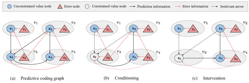
Figure 2: $(a)$ PC graph with the same causal structure of that in Fig.1. Every vertex $v_{i}$ of the graph is associated with a value node $\mathbf{x}_{i}$, and an error node $\mathbf{e}_{i}$. The arrows show the influence of every node of the graph to the others: the prediction information follows the direction of the arrows of the original graph, while the error information goes backwards. $(b)$ Example of conditioning in PC graphs. Here, we fix the value of $\mathbf{x}_{3}$, making the effect of all the arrows entering $v_{3}$ irrelevant, as $\mathbf{x}_{3}$ is fixed and hence does not change accordingly to in-coming information anymore. This, however, does not apply to error information going out from $v_{3}$, which keeps influencing $\mathbf{x}_{1}$ and $\mathbf{x}_{2}$. This is solved in $(c)$, where we provide an example of an intervention in PC graphs. According to Pearl’s causal theory, the do-operator on a specific node ($v_{3}$ in this case) removes the incoming edges, to avoid the newly introduced information to flow backwards and influence the parent nodes. As in predictive coding, the only information flowing opposite to the causal relations is the error information, an intervention can simply be performed by removing (or setting to zero) the error node.

The main goal of causal inference is to be able to simulate intervenions in a process, and study the counterfactual effects of such interventions. In statistics, interventions are denoted by the $do(-)$ operator (Pearl, 1995, 2009). The value of a random variable $\mathbf{x}_{i}$ when performing an intervention on a different variable $\mathbf{x}_{j}$ is denoted by $p(\mathbf{x}_{i}\mid do(\mathbf{x}_{j}=\mathbf{s}))$. This is equivalent to the question What would $\mathbf{x}_{i}$ be in this environment if we set $\mathbf{x}_{j}=\mathbf{s}$? In the case of the example in Fig. 1, the question could be What would the expected income level be, if we change the education level of this person? In fact, while ‘education’ and ‘income level’ may be correlated by a hidden confounder (intelligence, in this case), an intervention removes this correlation by changing the education level of a randomly selected individual, regardless of level of intelligence.

To perform an intervention on a Bayesian network, we first have to act on the structure of the graph, and then query the model by conditioning on the new graph, as shown in Fig. 1. Assume that we have a graph $G$, and we want to know the value of $\mathbf{x}_{i}$ after performing an intervention on $\mathbf{x}_{j}$, by fixing it to some value $s$. This can be done according to the two following steps:

1. Generate a new graph $G^{\prime}$ by removing all the in-coming edges of $v_{i}$ from $G$.

2. Compute the conditional expectation $E(\mathbf{X}\mid\mathbf{x}_{j}=\mathbf{s})$ using $G^{\prime}$.

Interventional query.

We now show how to perform an intervention on a PC graph. Here, the only information that flows in the opposite direction of an arrow is the prediction error. In fact, if we have $v_{1}\rightarrow v_{2}$, the update of the value node $\mathbf{x}_{1}$ is affected by the error $\mathbf{e}_{2}$. This can be avoided by simply fixing the prediction error of $\mathbf{e}_{2}$ to zero throughout the inference phase. This is convenient, since it allows us to not directly act on the structure of the graph to perform interventions but rather perform them dynamically ‘at runtime’, which results in increased efficiency in the case of nodes with a large number of incoming edges. Hence, we have the following:

$$E(\mathbf{x}_{i}\mid do(\mathbf{x}_{j}=\mathbf{s}))=E(\mathbf{x}_{i,T}\mid\forall t:\mathbf{x}_{j,t}=\mathbf{s},\mathbf{e}_{j,t}=0).$$ (6)

3.1 Structural Causal Models

To determine the outcome of a specific action, it is imperative to carry out an intervention and monitor the resulting effects. Consequently, interventions serve as a tool to address queries about outcomes of interventions in the present. Conversely, counterfactuals are used to study the impact of interventions in the past. Given that the action resides in the past, counterfactuals inherently lack observability of the causal effect. Counterfactual inference can, however, use structural causal models (SCMs). An SCM is a triple $(U,V,F)$, where $V$ is a set of endogenous (observable) variables, which represent the internal vertices of the graph, and $U$ a set of exogenous (unobservable) variables, representing the roots of the graph, i.e., vertices with no parents. To conclude, $F$ is a set of functions that determine the predicted values of the endogenous variables according to the structure of $G$. We denote the value nodes of the exogenous variables by $\mathbf{u}_{1},\dots,\mathbf{u}_{M}$. An SCM can then be used to model counterfactuals, i.e., answers to the question What would $\mathbf{x}_{i}$ be, had $\mathbf{x}_{j}$ been equal to $\mathbf{s}^{*}_{j}$ in situation $U=\mathbf{u}$? In our case, What would the income of this person have been, had his education level been a master degree in situation $U=\mathbf{u}$? Here, $\mathbf{u}$ could be a specific year/period with information about how much people with a specific job would be paid. To compute this, three steps are needed:

1. Abduction: Here, we are provided with values $(\mathbf{s}_{1},\dots,\mathbf{s}_{N})$ for all the internal nodes in $V$. We use them to compute the values of the exogenous variables, which we denote by $\tilde{u}_{1},\dots,\tilde{u}_{M}$. Hence, according to the following:

   $$E(\mathbf{u}_{1},\dots,\mathbf{u}_{M}\mid\forall t:(\mathbf{x}_{1},\dots,\mathbf{x}_{N})=(\mathbf{s}_{1},\dots,\mathbf{s}_{N})).$$ (7)

2. Action: Now that we computed the values of the exogenous variables, we fix them and perform an intervention on $\mathbf{x}_{j}$. Particularly, we set $\mathbf{x}_{j}=\mathbf{s}^{*}_{j}$, and we set $\mathbf{e}_{j}=0$, which has the effect of removing any influence of $x_{j}$ on its parent nodes.

3. Prediction: We now have all the elements to compute the counterfactual on $\mathbf{x}_{i}$, which is:

   $$E(\mathbf{x}_{i}\mid\forall t:(\mathbf{u}_{1},\dots,\mathbf{u}_{M})=(\tilde{\mathbf{u}}_{1},\dots,\tilde{\mathbf{u}}_{M}),\ \mathbf{x}_{j}=\mathbf{s}^{*}_{j},\ \mathbf{e}_{j}=0).$$ (8)

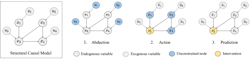
Figure 3: What would $\mathbf{x}_{4}$ be, had $\mathbf{x}_{3}$ been equal to $\mathbf{s}^{*}_{3}$ in situation $U=\mathbf{u}$? This figure provides an example of the three-step process to perform counterfactuals, using a structural causal model with four exogenous and four endogenous variables. We are given two kinds of data: the original values of $\mathbf{x}_{1},\dots,\mathbf{x}_{4}$, which correspond to past information, here denoted by $\mathbf{s}_{1},\dots,\mathbf{s}_{4}$, and the intervention information $\mathbf{s}_{3}^{*}$, needed to understand the what would have happened to $\mathbf{x}_{4}$ if we had changed $\mathbf{s}_{3}$ to $\mathbf{s}_{3}^{*}$?. The final answer corresponds to the node $\tilde{\mathbf{x}}_{4}$ obtained in the prediction step.

3.2 Experiments

We now perform a series of experiments that confirm the theoretical claims made in the previous section, as well as showing possible applications of the proposed method. We divide the experiments into three groups: causal inference, classification, and robustness. In detail, we empirically demonstrate the correctness of our claims, and discuss the potential applications in machine learning. To this end, we test PC graphs on the three levels of Pearl’s ladder of causation [2009], namely, association (statistical, at level 1), intervention (level 2), and counterfactual (at level 3). Then, we show how interventions can be used to improve the performance of classification tasks on fully connected models. We conclude with an experiment showing the robustness of PC graphs when performing counterfactual inference on more complex tasks. A more detailed presentation of the experiments, as well as all the details needed to reproduce the results, are given in the supplementary material.

Causal Inference.

We test interventional and counterfactual query capabilities based on different common causal graph structures, namely, (i) collider ($N=3$), (ii) confounder ($N=3$), (iii) mediator ($N=3$), (iv) chain ($N=3$), (v) fork ($N=3$), (vi) M-bias ($N=5$), and (vii) butterfly bias ($N=5$), an extension of M-bias that is sometimes called bow-tie bias. Given a linear SCM with additive Gaussian noise (for one of the structures above), we generate observational training data, as well as associational, interventional, and counterfactual test datasets. First, the observational data is generated by randomly sampling values for the exogenous variables $\mathbf{u}$. We then use the exogenous values to compute the values of the endogenous variables $\mathbf{x}_{i}$. Second, for interventional data, we follow a similar procedure, but the structural equations are altered by an intervention. Finally, the counterfactual data consist of pairs, ($\mathbf{x},\mathbf{x}^{\prime}$) with $\mathbf{x}$ being observational data and $\mathbf{x}^{\prime}$ interventional data, both sharing the same $\mathbf{u}$. To perform causal inference, we fit the predictive coding network to the observed data to learn the parameters of the structural equations including the noise distribution parameters. We evaluate the learned SCM by comparing a metric, e.g., the Mean Absolute Error (MAE), between the true and inferred values for association, intervention, and counterfactual queries. We refer the reader to the appendix for more details on the various metrics used.

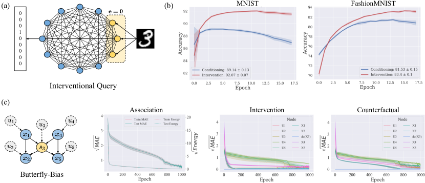
Figure 4: (a) How to compute a prediction given a data point on a fully connected PC graph, using interventional queries. (b) Plots of test accuracies over epochs obtained using conditional and interventional queries on the same trained model. (c) Left to right: causal structure of the underlying SCM. Convergence behaviour of predictive coding energy vs. error metric, MAE, during SCM learning for butterfly bias DAG. Error of interventional query estimates by node for intervention on $\mathbf{x}_{3}$ (yellow node in DAG). Error of counterfactual query estimates by node for counterfactuals with intervention on $\mathbf{x}_{3}$ and given factual data (colored nodes in DAG).

Here, we only provide results for the most interesting and complex graph among the proposed ones, namely, the butterfly bias. In Section A, we provide a detailed study of all the aforementioned graphs, on a large number of metrics. The results show that PC graphs are able to estimate accurate distributions for all nodes in the causal graph in both the interventional and the counterfactual setting, and that our proposed approach allows for SCMs with arbitrary Gaussian distribution. The plots in Fig. 4(c) show that the model is able to correctly infer interventional and counterfactual queries, as shown by the converging MAE of non-intervened nodes.

Classification.

In the original work on PC graphs (Salvatori et al., 2022a), the authors have trained a fully connected model to perform classification tasks using conditional queries. The performances are poor compared to those of hierarchical models for two reasons: First, conditional queries do not impose any direction to the information flow, making the graph learn $p(\bf{y}|\bf{x})$ as well as $p(\bf{x}|\bf{y})$, even though we only need the first term. Similarly, the model also learns $P(\mathbf{x})$ and $P(\bf{y})$, which is, how the prior depends on itself. Second, the model complexity is too high, not allowing the model to use any kind of background knowledge, such as hierarchical/structural information/prior, usually present in sparser models. Here, we address the first limitation by performing an intervention on the input: this prevents the error of the inputs to spread in the network, and enforces a specific direction of the information flow, which goes from cause (the image) to effect (the label). To assess the impact of such an intervention on the test accuracy, we train a fully connected model with $2000$ neurons on the MNIST and FashionMNIST datasets, and compute the test accuracy for conditional and interventional queries. We perform a large hyperparameter search on learning rates, activation functions, and weight decay values. In all cases, performing an intervention improves the results. In Fig. 6(d), we present an example showcasing the best results obtained after hyperparameter search. The interventional query led to improvements in the final test accuracy of almost $2\%$ for both datasets. Additional experiment details can be found in the supplementary material.

Robustness.

A recent work demonstrates that existing deep-learning methods fail to obtain sufficient robustness or performance on counterfactual queries in certain scenarios (De Brouwer, 2022). To address this limitation, the authors proposed a new technique to overcome these shortcomings. We show that predictive coding surpasses current state-of-the-art results for counterfactual queries while requiring a simpler architecture without relying on ad hoc training techniques. We evaluate the robustness of our model on counterfactual inference tasks of higher dimensions, thereby examining the feasibility of our method to perform causal inference on more complex data. The dataset that we consider here consists of tuples $(\mathbf{x},\mathbf{u}_{z},\mathcal{T},\mathbf{y},\mathcal{T}^{\prime},\mathbf{y}^{\prime})$, where $\mathbf{x}$ is an image from the MNIST dataset, $\mathcal{T}$ is the assigned treatment, which is a rotation angle (confounded by $\mathbf{x}$). Furthermore, $\mathbf{u}_{z}$ is a hidden exogenous random variable that determines the color of the observed outcome image $\mathbf{y}$, that is added to the forth variable $\mathbf{y}^{\prime}$, a colored and rotated MNIST image representing the counterfactual response obtained when applying the alternative treatment $\mathcal{T}^{\prime}$. We consider SCMs with $4$ nodes that encode the four variables, as sketched in Fig. 5. Here, every edge represents a feed-forward network of different depth and hidden dimension $1024$. We perform a large hyperparameter search, and a detailed explanation of how to reproduce the results are given in the supplementary material.

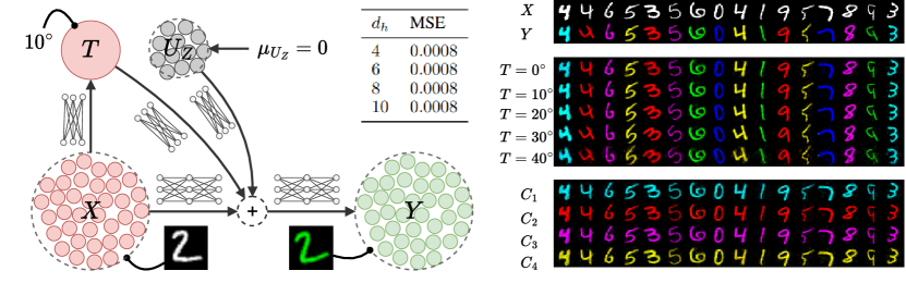
Figure 5: Architecture used to reconstruct counterfactual images. $U_{Z}$ corresponds to the color of the digit, $T$ to the rotation angle, $X$ to the input, $Y$ to the colored and rotated image. The colored digits show that our method is robust when performing interventions on the rotation angle. The table shows that the model performance does not depend on the choice of the number of neurons for the node $\mathbf{u}_{z}$. The work proposing the experiment (De Brouwer, 2022) reports an MSE of $0.001$.

Results.

The results show that PC graphs improve on state-of-the-art methods, despite the fact that we do not use convolutional layers like in the original work. First, the generated images have an MSE on the test set ($0.0008\pm 0.0002$) that is lower than that reported in the original work ($0.001\pm 0.001$). The high quality of reconstruction is also visible in the generated images reported in Fig. 5. Compared to the work (De Brouwer, 2022), we are able to generalize to rotations of $40^{\circ}$, even if this introduces some noise in the generated output. Furthermore, contrary to the original model, our architecture is robust with respect to the choice of the hyperparameter linked to $u_{z}$ and does not necessitate to perform a hyperparameter sweep to find the right value. Hence, we conclude that PC graphs are able to correctly model the treatment rotation in the counterfactual outcome, while keeping the color, which is independent of rotation, unchanged.

4 Structure Learning

Learning the underlying causal structure from observational data is a critical and highly active research area, primarily due to its implications for explainability and modeling interventions. Traditional approaches use combinatorial search algorithms to find causal structures. However, such methods tend to become computationally expensive and slow as the complexity (e.g., the number of nodes) of the graph increases, as shown in previous works (Chickering, 1996, 2002). Therefore, we focus on gradient-based learning methods instead (Zheng et al., 2018), as these allow us to handle larger causal graph structures in a computationally efficient manner. Let us consider $\mathbf{A}$ to be the adjacency matrix of a graph. Ideally, this matrix should be a binary matrix with the property that $a_{i,j}=1$, if there exists an edge from $v_{i}$ to $v_{j}$, and $0$, otherwise. In this work, however, we adopt a Bayesian perspective. We regard $\mathbf{A}$ not as a static matrix but as a matrix composed of continuous, learnable parameters, which assign weights to signify the importance of specific connections. To this end, we can consider every predictive coding graph to be fully connected, where the prediction of every node $\mathbf{x}_{i}$ now depends on the entries of the adjacency matrix:

$$\bm{\mu}_{i}=\textstyle\sum_{k=0}^{N}a_{k,i}f_{k,i}(\mathbf{x}_{k}),\ \ \ \ \ \ \ \ \ \ \mathrm{update\ rule:}\ \ \ \Delta a_{i,j}\propto-\frac{\partial F}{\partial a_{i,j}}=\beta\cdot\mathbf{e}_{i,T}\mathbf{W}^{\top}f(\mathbf{x}_{j,T}),$$ (9)

where $\beta$ is the specific learning rate of the parameters of $\mathbf{A}$. With this formulation, the entries of $\mathbf{A}$ are updated via gradient descent to minimize the variational free energy of Eq. 2. Our goal is to learn an acyclic, sparsely connected graph, which requires a prior distribution that enforces these two constraints. We consider three possible priors: a Gaussian prior, a Laplace prior, and the acyclicity prior. The latter prior is equal to zero if and only if the corresponding graph is acyclic (Zheng et al., 2018):

$$l(\mathbf{A})=exp(-\textstyle\sum_{i,j}|a_{i,j}|),\ \ \qquad g(\mathbf{A})=\mathcal{N}(0,1),\ \ \qquad h(\mathbf{A})=tr(exp(\mathbf{A}\times\mathbf{A}))-d.$$

The energy function that we aim to minimize via gradient descent is given by the sum of the total energy, as defined in Eq. 2, and the three aforementioned prior distributions, each weighted by a scaling coefficient. The first two priors effectively apply the $L1$ and $L2$ norms to the parameters of the adjacency matrix, and they form the elastic norm when used in conjunction.

Negative Examples.

The regulariser $h(A)$ introduces an inductive bias that may be undesirable, as we know that cyclic structures, such as lateral connections, are beneficial in several tasks (Salvatori et al., 2022a). Without $h(A)$, however, training converges towards a degenerate structure, where each output node predicts itself, ignoring any contribution of the input nodes. We solve this degeneration behavior by introducing negative examples, which are data points with a wrong label, into the training set. The model is then trained in a contrastive way (Chen et al., 2020), i.e., by increasing the prediction error of every node for negative examples $k$, and decreasing it otherwise, when the label is correct, as shown in Fig. 6(c). A detailed explanation of how training with negative samples works, as well as examples of degenerate structures learned when training without the acyclicity prior, are given in the supplementary material. We show that negative examples address the convergence issue towards a degenerate graph by rendering the label nodes contingent on the inputs, thus steering the model towards adopting a hierarchical structure instead.

4.1 Experiments

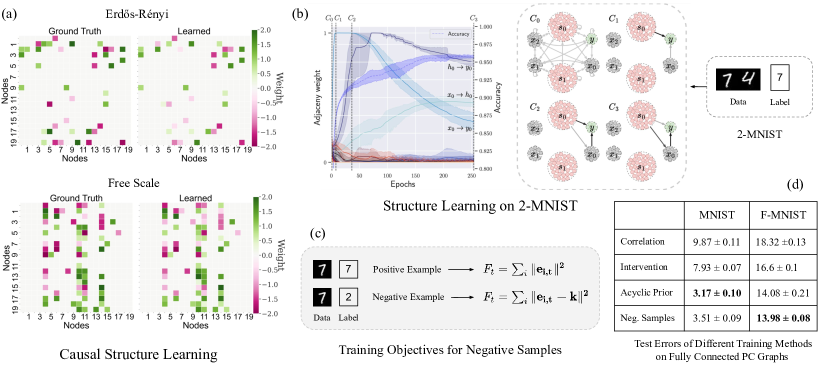
Figure 6: (a) Experiments on structure learning from synthetic data, generated from Erdős-Rényi and scale-free random graphs with $20$ nodes. On the left, the connection strength of the true graph; on the right, the one learned by a PC graph. (b) Structure learning on the $2$-MNIST dataset: the plot shows the weights of the adjacency matrix $\mathbf{A}$ over the number of epochs, the sketch on the right the resulting PC graph. (c) A description of the two energy functions optimized by the PC graph when training on negative and non-negative examples. (d) Table with test error of all experiments performed on MNIST and FashionMNIST, averaged over three seeds. The best results are obtained when augmenting the training process with both the proposed structure learning methods.

We perform two different structure learning experiments. In the first experiment, we assume that we are provided with a dataset generated by a Bayesian network with one-dimensional nodes and unknown causal structure. The task is then to retrieve the original graph from a fully connected predictive coding graph. This is a standard task in causal discovery (Morales-Alvarez et al., 2022; Geffner et al., 2022b; Zheng et al., 2018). In the second experiment, we perform classification for MNIST and FashionMNIST using a fully connected predictive coding graph. This time, however, we augment the classification objective with priors to enforce sparsity and acyclicity, and conjecture that $(i)$ this will improve the final test accuracy, and $(ii)$ reduce a fully connected graph to the “correct” sparse network, i.e., the hierarchical one.

4.1.1 Structure Learning

For the following experiment, we use synthetic data, sampled from an SCM with $N\in\{10,15,20\}$ nodes and a graph with either $2N$ or $4N$ expected edges. The graph structure is either of an Erdős-Rényi or a scale-free random graph. To this end, we denote an Erdős-Rényi graph with $2N$ expected edges as ER2, while SF4 denotes a scale-free graph with expected $4N$ edges, for example. We vary the number of nodes and edges to demonstrate the versatility and robustness of our method in handling various graph structures. Next, we place uniformly random edge weights onto the binary adjacency matrix of a graph, to obtain a weighted adjacency matrix, $\mathbf{W}$. Finally, we sample observational data based on a set of linear structural equations with additive Gaussian noise, $\mathbf{u}\sim\mathcal{N}(\mathbf{0},\mathbf{I}_{N})$, such that

$$\mathbf{x}=\mathbf{W}^{T}\mathbf{x}+\mathbf{u}\in\mathbb{R}^{N}.$$

As each node is one dimensional, we can set without loss of generality the parameters of the adjacency matrix to be the actual parameters $\mathbf{W}$ of the fully connected PC model. To prune the parameters that are not used in the linear structural equations that generate the observed data, we require our model to be sparse and acyclic. Hence, we consider the parameters to have prior distributions $h(\mathbf{W})$ and $l(\mathbf{W})$. Then, the experiment consists of training the fully connected model to fit the dataset, and checking whether the predictive coding graph can converge to the random graph structure that initially generated the data.

Results.

The results show that PC graphs are able to learn the causal structure for arbitrary dense graphs of various sizes. The heatmaps in Fig. 6(a) show that PC graphs are able to estimate the true weight adjacency matrix for dense SF4 and ER2 graphs with $20$ nodes. Hence, we conclude that the learned adjacency matrix, which we chose as the median performing model across multiple runs, is able to well capture the causal dependencies in the considered datasets. More details on how the datasets are generated, on how the experiment is performed, a table with quantitative results showing the performance, as well as a detailed comparison against multiple baselines (PC (Kalisch and Bühlman, 2007), GES (Chickering, 2002), NOTEARS (Zheng et al., 2018), and ICALiNGAM (Shimizu et al., 2006)), are given in the supplementary material. In contrast to the baselines that display inconsistent results across graphs, our method sustains a stable and competitive performance in all ER and SF graph setups, as validated by the structural Hamming distance (SHD), F1 score, and other supplementary accuracy metrics.

4.1.2 Classification

Here, we extend the study on the experiments performed in Section 3, and check whether we are able to improve the results by allowing the predictive coding graph to cut extra connections during training. Additionally, we create a new dataset, called $2$-MNIST, whose data consist of pairs $(\mathbf{s}_{0},\mathbf{s}_{1})$ of MNIST images, and the label is the label of $\mathbf{s}_{0}$. This is to check whether predictive coding networks are able to understand the underlying causal structure of the dataset, and remove connections that start from $\mathbf{s}_{1}$. As an architecture, we consider a predictive coding graph with $6$ nodes, one of dimension $784$, one of dimension $10$, and $4$ hidden nodes of dimension $d$. In the case of $2$-MNIST, we have two nodes of dimension $784$, and only three of dimension $d$. The adjacency matrix $\mathbf{A}$ has then dimension $6\times 6$. Note that, when the entries of $\mathbf{A}$ are all equal to one, then this model is equivalent to the fully connected one of Section 3. Here, however, we propose two techniques to augment the training process, and let the model converge to a hierarchical network. The first one consists of adding the three proposed priors on the matrix $\mathbf{A}$, to enforce sparsity and acyclicity in the graph; the second one consists of augmenting the dataset via negative examples, while enforcing sparsity via the Laplace prior only.

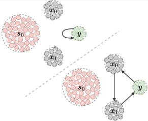
Figure 7: Examples of degenerate networks, where the label predicts itself either via self loops, or via cycles.

Degenerate Example. We start our discussion by showing a degenerate example, which arises when we do not use either negative examples, or a prior that forces an acyclic structure, but only the prior $l(A)$ which enforces sparsity. In this case, the modes is unable to learn the causal dependency between input and output, and converges towards a degenerate structure, where each output node predicts itself via a cyclic structure, which can be a self loop, or a closed loop with length larger than one. As each node either predicts itself or is unused, the total variational free energy of the network is going to be close to $0$, despite the network being randomly guessing the output. An example of such structures is provided in Figure 7. This shows the importance of additional methods, that force the network to be aware of the causal dependency between the input and the output. We now test the two proposed methods: the acyclic prior, and the use of negative examples.

Setup.

In the first experiment, we use the $2$-MNIST dataset to test whether the acyclic and sparse priors are able to both remove the out-going connections from the second image $\mathbf{s}_{2}$, and learn a hierarchical structure, which we know to be the best one to perform classification on MNIST. In the second experiment, we train the same fully-connected model of Section 3 and check whether the priors allow to increase the classification accuracy of the model. To conclude, we perform a classification task with the negative examples and the Laplace prior, to test whether this method also allows to avoid converging to degenerated graph structures.

Results.

The results on the $2$-MNIST dataset show that the model immediately prunes the parameters out-going from $\mathbf{s}_{2}$. In the first $~{}100$ epochs, the edge with the largest weight is the linear one, which directly connects the input to the label. While this shows that the model correctly learned the dependencies, linear classification on MNIST and FashionMNIST does not yield great accuracies. This problem is naturally addressed in the later stages of the training process, where the entry of the adjacency matrix relative to the linear map loses weights, and hence influence on the final performance of the model. When training finally converges, the resulting model is hierarchical, with one hidden layer, as shown in the plot in Fig. 6(b). This shows that PC graphs are not only able to learn the causal dependencies correctly, but also to be able to discriminate among these structures, and converge to a well performing one.

In the second experiment, where we perform classification on MNIST and FashionMNIST with $h(\mathbf{A})$, the model shows a clear improvement over the baseline proposed in Section 3. The same applies for the training with negative examples, as reported in the table in Fig. 6(d), which shows a performance comparable to these of training with an acyclicity prior. To reach the usual results that can be obtained via standard neural networks trained with backpropagation (i.e., a test error $<2\%$), it suffices to fine-tune the model using the newly learned structure.

5 Related Work

In recent years, there have been a large number of works that have tackled machine learning problems using predictive coding networks. They have been shown to perform relatively well in classification tasks using all kinds of architectures, such as feedforward models, convolutional networks, graph neural networks, and transformer models (Whittington and Bogacz, 2017; Han et al., 2018; Salvatori et al., 2022c; Byiringiro et al., 2022; Pinchetti et al., 2022). These results are partially justified by some similarities that predictive coding shares with backpropagation when performing supervised learning (Song et al., 2020; Millidge et al., 2020; Salvatori et al., 2022b). Multiple works have also applied it to tasks such as image generation (Ororbia and Kifer, 2022; Ororbia and Mali, 2019), continual learning (Ororbia et al., 2022; Song et al., 2022), and associative memories (Salvatori et al., 2021; Yoo and Wood, 2022; Tang et al., 2023).

Causality has found applications in problems such as treatment effect estimation, time series modeling, image generation, and natural language processing, as well as enhancing interpretability and fairness in machine learning (Shalit et al., 2017; Runge et al., 2019; Lopez-Paz et al., 2017; Kaushik et al., 2019; Kusner et al., 2017). Different works have used deep generative modeling techniques to investigate causality problems, such as graph neural networks, variational autoencoders, and flow and diffusion models (Sanchez and Tsaftaris, 2022a; Khemakhem et al., 2021; Karimi et al., 2020; Pawlowski et al., 2020a; Yu et al., 2019). Some works study the problem of learning the causal structure from observational data, previously done via combinatorial search (Spirtes et al., 2000; Chickering, 2002; Shimizu et al., 2006; Kalisch and Bühlman, 2007). However, combinatorial search algorithms grow double exponentially in complexity with respect to the dimension of the graph. To this end, recent works mostly performing continuous optimization by using the acyclic prior that we have also discussed in our work (Zheng et al., 2018; Bello et al., 2022; Yu et al., 2019).

Most recently, end-to-end approaches for causality have emerged, combining causal discovery and causal inference tasks into a unified deep learning pipeline (Sharma and Kiciman, 2020; Geffner et al., 2022b; Khemakhem et al., 2021). Our predictive coding approach follows a similar path, concurrently addressing both tasks in a single framework. However, we differ from the existing methodologies in that we neither require a pipeline of deep neural networks (Geffner et al., 2022a) nor do we need to simplify the causal graph to its non-unique causal ordering (Khemakhem et al., 2021) for executing causal discovery and inference.

6 Conclusion

In this work, we have provided a bridge between the fields of causal inference and computational neuroscience. In detail, we have shown that predictive coding graphs have the ability of both learning the causal structure from observational data, and modeling associational, interventional, and counterfactual distributions (Geffner et al., 2022b; Sharma and Kiciman, 2020). This makes it an end-to-end causality engine, which can answer causal queries without knowing the child-parent relationships in the structural equations of the SCM. In the case of causal inference, we have shown how interventions can be performed by simply setting prediction errors of nodes that we are intervening on to zero, and how this leads to the formulation of predictive-coding based structural causal models. For structure learning, we have shown how to use existing techniques to derive causal relations from data. More generally, this work further highlights the flexibility of predictive coding models, which can be used to both train deep neural networks that perform relatively well in different machine learning tasks, and to perform Bayesian and causal inference on directed graphical models.

Appendix

Appendix A Interventional and Counterfactual Inference

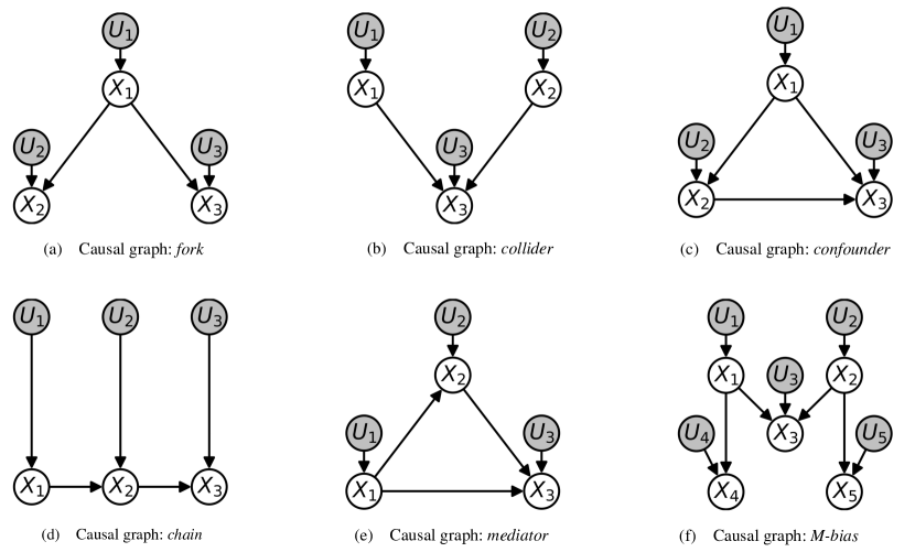
Figure 8: Additional graph structures used in experiments of Section 3. White nodes are endogenous variables and observed. Shaded nodes denote independent, exogenous variables for which we do not observe data unless they have no parents in which case $\mathbf{x}_{i}\coloneqq\mathbf{u}_{i}$.

Here, we provide a detailed discussion on the experiments proposed in Section 3, where we test the ability of PC graphs to model interventional and counterfactual queries. The core of decision making is to be able to determine which intervention/action results in an outcome of interest. As such, being able to answer causal queries on a variety of DAG structures and intervention nodes in a DAG is essential. The causal inference approach that we propose only requires knowledge of the causal structure in the form of parent-child relationships among endogenous variables $\mathbf{x}$. We assume the parameters of the structural equations, $F$, to be unknown. We make the causal sufficiency assumption, meaning that there is no hidden confounding [Peters et al., 2017]. This is achieved by having an independent exogenous variable, $\mathbf{u}_{i}$, for each endogenous node, $\mathbf{x}_{i}$.

Setup.

We test the associational, interventional, and counterfactual query capabilities of our method on different common causal graph structures with $N$ endogenous nodes, namely (i) collider ($N=3$), (ii) confounder ($N=3$), (iii) mediator ($N=3$), (iv) chain ($N=3$), (v) fork ($N=3$), (vi) M-bias ($N=5$), and (vii) butterfly bias ($N=5$). Each of these structures is visualized in Fig. 8. For every structure, we generate datasets from a linear SCM with additive Gaussian noise and no restrictions on the location and scale parameters. We use observational training data, $\mathbf{X}$, to fit the PC model. We learn each structural equation, $F_{i}$, via a training scheme in which we infer the exogenous variables, $\mathbf{u}$, given observed endogenous variables, $\mathbf{x}$, from the training dataset. As such, the SCM is fitted by estimating the parameters of each exogenous variable according to $\mathbf{u}_{i}\sim\mathcal{N}(\bm{\mu}_{i},\sigma_{i})$. This way, we learn to approximate the distribution of the SCM’s exogenous variables $\mathbf{u}$. Note that during the training process, we do not use the factual data once the abduction step is completed. Instead, we replace node values of factual data with inferred values, $\hat{\mathbf{x}}$, by applying the currently learned set of structural equations $\hat{F}$ to the inferred exogenous node values, $\hat{\mathbf{u}}$. We use associational (obs), interventional (do), and counterfactual (cf) test datasets $\{\mathbf{X}^{obs}$, $\mathbf{X}^{do}$, $\mathbf{X}^{cf}$ } to evaluate our method. The interventions required for $\mathbf{X}^{do}$ and $\mathbf{X}^{cf}$ are randomly sampled from $\bm{\mu}_{i}+\sigma(\mathbf{x}_{i})\times\{-1.0,-0.5,-0.1,0,0.1,0.5,1.0\}$ to ensure realistic intervention values in the support of the each observed marginal distribution. Here, $\bm{\mu}_{i}$ and $\sigma(\mathbf{x}_{i})$, represent the empirical mean and standard deviation of $\mathbf{x}_{i}$ from the training data. To generate an interventional or counterfactual sample, we perform do-operation on individual nodes only, one variable at a time.

For every SCM, we repeat experiments over five different seeds, each using a different PC model initialization. We report error metrics with mean and standard deviation, both multiplied by 100 for clarity. The PC graph is trained with $3000$ samples for $1000$ epochs with a batch size of $128$. We use the vanilla stochastic gradient descent (SGD) optimizer for the node values with a learning rate of $\gamma=3e-3$ and $T=8$ iterations for inference of node values during training and testing. For the weights, we use the AdamW optimizer with a learning rate of $\alpha=8e-3$ and a weight decay of $\lambda_{w}=1e-4$. We fit the model using one-dimensional linear layers for each connection between the endogenous and exogenous variables of the SCM according to the causal structure defined given by the adjacency matrix $\mathbf{A}$. Our approach does not require the use of neural networks with many hidden layers. This makes our causal PC graph efficient and lightweight, because we only learn the parameters that define the structural equations $F$ of the true data generating SCM. Note that, despite the large amount of epochs considered, every model converges in less than two minutes. All results are averaged over five random seeds.

Metrics.

We now specify the metrics used to evaluate performance in estimating associational, interventional, and counterfactual distributions, as detailed in Section 3. Observational metrics are computed by comparing the true and estimated values of exogenous variables, using the available endogenous node data. Furthermore, note that for interventions and counterfactuals only the descendants, $des(\mathbf{x}_{i})$, of an intervened node $\mathbf{x}_{i}$ are affected. Therefore, the causal order of a DAG becomes important when assessing performance on interventional and counterfactual queries. As such, we report metrics with respect to the descendants of the intervention node, as per the adjacency matrix. We follow the works in the related literature [Sánchez-Martin et al., 2022, Chao et al., 2023] and report the following metrics:

• mean absolute error (MAE),

• maximum mean discrepancy (MMD) [Gretton et al., 2012],

• estimation squared error for the mean (MeanE),

• estimation squared error for standard deviation (StdE),

• mean of the squared error (MSE),

• standard deviation of the squared error (SSE).

We use MAE as a generic metric to assess the error between the estimated query and the ground truth query. The MMD metric is a sample-based distance measure between distributions. We use MMD to assess the match between the estimated distribution and the true distribution. The idea is to compare the means of both samples, $\widehat{\mathbf{X}}$ and $\mathbf{X}$, in a higher-dimensional feature space defined by a kernel function $k$.

For a pair of samples from each distribution, we compute the MMD as follows:

$$\text{MMD}(\mathbf{X},\widehat{\mathbf{X}}) =\left\lVert\frac{1}{M}\sum_{i=1}^{M}\phi(\mathbf{x}^{i})-\frac{1}{M}\sum_{i=1}^{M}\phi(\hat{\mathbf{x}}^{i})\right\rVert^{2}$$ (10)

$$=\frac{1}{M^{2}}\sum_{i=1}^{M}\sum_{j=1}^{M}k(\hat{\mathbf{x}}^{i},\hat{\mathbf{x}}^{j})-\frac{2}{M^{2}}\sum_{i=1}^{M}\sum_{j=1}^{M}k(\mathbf{x}^{i},\hat{\mathbf{x}}^{j})+\frac{1}{M^{2}}\sum_{i=1}^{M}\sum_{j=1}^{M}k(\mathbf{x}^{i},\mathbf{x}^{j}).$$ (11)

Here, $\phi$ is the feature map of the kernel function $k$, and $\mathbf{x}^{i}$ and $\hat{\mathbf{x}}^{i}$ are the $i$-th samples from the ground truth and the inferred data, respectively. Each $\hat{\mathbf{x}}^{i}$ and $\mathbf{x}^{i}$ is a vector of $N$ features, one for each endogenous node in the DAG. The kernel function $k$ measures the similarity between data points in the feature space. In our implementation, we use a mixture of RBF (Gaussian) kernels with varying bandwidth parameters [Gretton et al., 2012].

We use MeanE and StdE to assess the estimated interventional distributions. MeanE and StdE measure the average squared error between the true and estimated mean and standard deviation of an interventional distribution, respectively. Both metrics are computed as averages across a set of intervention indices, $\mathcal{I}$, that correspond to nodes in the DAG that have descendants and thus are not leaf nodes.

Given the empirical means, $E\left[\mathbf{x}_{i}|do(\mathbf{x}_{j})\right]$ and $E\left[\hat{\mathbf{x}}_{i}|do(\mathbf{x}_{j})\right]$, and the empirical standard deviations, $SD\left[\mathbf{x}_{i}|do(\mathbf{x}_{j})\right]$ and $SD\left[\hat{\mathbf{x}}_{i}|do(\mathbf{x}_{j})\right]$, for node, $\mathbf{x}_{i}$, with intervention on node, $\mathbf{x}_{j}$, with index $j$, the MeanE and StdE are computed in the following way:

$$\text{MeanE}=\frac{1}{|\mathcal{I}|}\sum\limits_{j\in\mathcal{I}}\frac{1}{|des(j)|}\sum\limits_{i\in des(j)}{\left(E\left[\mathbf{x}_{i}|do(\mathbf{x}_{j})\right]-E\left[\hat{\mathbf{x}}_{i}|do(\mathbf{x}_{j})\right]\right)}^{2},$$ (12)

$$\text{StdE}=\frac{1}{|\mathcal{I}|}\sum\limits_{j\in\mathcal{I}}\frac{1}{|des(j)|}\sum\limits_{i\in des(j)}{\left(SD\left[\mathbf{x}_{i}|do(\mathbf{x}_{j})\right]-SD\left[\hat{\mathbf{x}}_{i}|do(\mathbf{x}_{j})\right]\right)}^{2}.$$ (13)

We denote the number of intervention nodes in the DAG as $|\mathcal{I}|$, and $des(j)$ is the the set of descendants of the intervention node with index $j$. Finally, to assess the performance for the counterfactuals, we report the MSE and SSE for the descendants of an intervention node with index $j$. Both metrics are computed as averages across all intervention nodes in $\mathcal{I}$. We use the Frobenius norm, $T_{j}=\|\mathbf{x}_{des(j)}-\hat{\mathbf{x}}_{des(j)}\|_{F}$, to measure the difference between true and estimated values of a counterfactual query with intervention on node index $j$. Defining the average of the empirical mean of $T_{j}$ as $E\left[T_{j}\right]$ and the average of the empirical standard deviation of $T_{j}$ as $SD\left[T_{j}\right]$, we retrieve the MSE and SSE metrics as:

$$\text{MSE}=\sum\limits_{j\in\mathcal{I}}\frac{1}{|des(j)|}\,E\left[T_{j}\right],$$ (14)

$$\text{SSE}=\sum\limits_{j\in\mathcal{I}}\frac{1}{|des(j)|}\,SD\left[T_{j}\right].$$ (15)

To summarize, for associational inference, we report MMD on the observational test set. For interventional inference, we report MMD, MeanE, and StdE. For counterfactual inference, we report MSE and SSE. Additionally, we report MAE on the associational and interventional inference as well as MSE and SSE for our method’s estimates of exogenous noise distributions, which are inferred in the abduction step while performing counterfactual inference. While not all the above metrics are required to evaluate a model’s causal inference performance, we still include them for benchmark comparison against state-of-the-art methods [Sánchez-Martin et al., 2022, Khemakhem et al., 2021, Karimi et al., 2020]. Across all metrics, lower values indicate better performance.

Appendix B Experiments on Common Causal Graphs

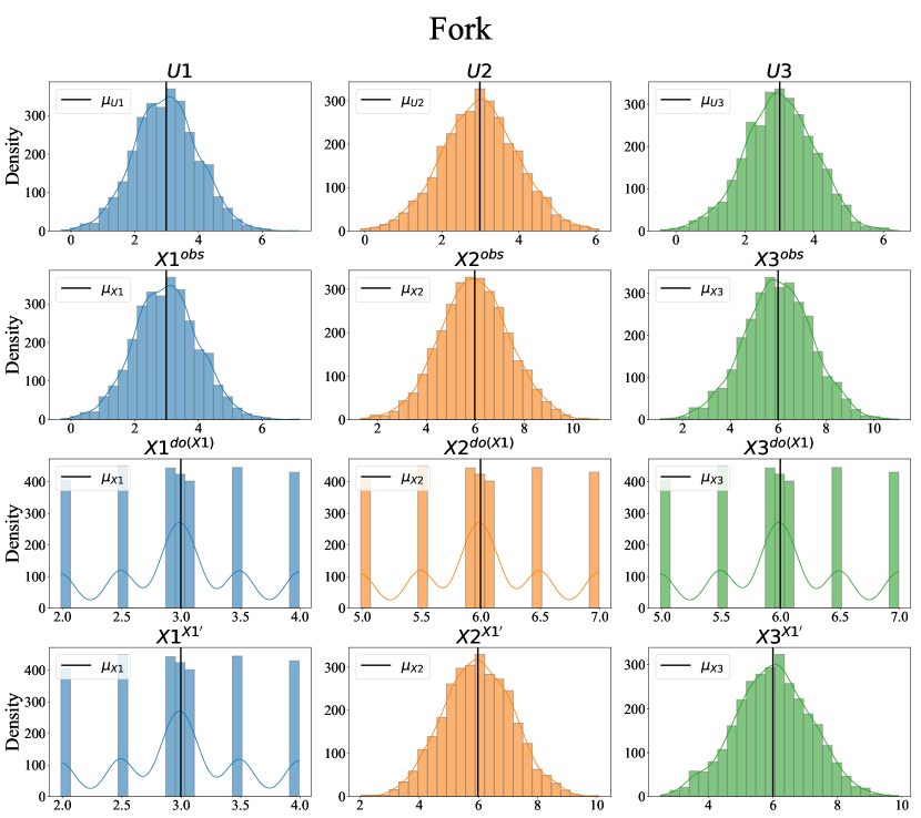
Figure 12: Causal hierarchy of distributions for fork SCM with intervention on $\mathbf{x}_{1}$. First row: Exogenous distribution. Second row: Associational distribution. Third row: Interventional distribution. Last row: Counterfactual distribution.

To generate data from a causal graph, we first sample a value for each of the $N$ exogenous variables that follow $\mathbf{u}_{i}\sim\mathcal{N}(\bm{\mu}_{i},\sigma_{i})$. Then, we use the deterministic structural equation, $F_{i}$, of node $\mathbf{x}_{i}$ to compute its value as $x_{i}\coloneqq F_{i}(par(x_{i}),\mathbf{u}_{i})$. Each $F_{i}$ is a linear equation with additive noise of the form $F_{i}=\sum_{j\in par(\mathbf{x}_{i})}w_{ji}\mathbf{x}_{j}+\mathbf{u}_{i}$, where $par(\mathbf{x}_{i})$ denotes the direct parents of node $\mathbf{x}_{i}$ according to the causal graph structures provided in Fig. 8. For the causal inference experiments with the common causal graphs in Fig. 8 as well as the butterfly bias DAG presented in the main body of the paper, we focused on performing interventions on nodes that are interesting. By interesting we mean that we want to show experimental results for interventions and counterfactuals on nodes that are neither root nodes nor leaf nodes. The reason being that interventions on such nodes either correspond to (a) regular conditional (associational) queries, as is the case with interventions on root nodes or (b) counterfactual queries that are not differentiable from interventional queries, as is the case for interventions on leaf nodes. Consequently, we provide results for the following causal inference scenarios: (i) chain graph with intervention on the middle node $\mathbf{x}_{2}$, (ii) confounder graph with intervention on confounding node $\mathbf{x}_{2}$, (iii) collider graph with intervention on root node $\mathbf{x}_{1}$ (colliders only contains root and leaf nodes), (iv) fork graph with intervention on root node $\mathbf{x}_{1}$, (v) mediator graph with intervention on the mediating node $\mathbf{x}_{2}$, (vi) M-bias graph with intervention on node $\mathbf{x}_{1}$, and finally (vii) butterfly bias graph with intervention on node $\mathbf{x}_{3}$. The $\mathbf{x}_{3}$ intervention on the butterfly bias is interesting and challenging, because $\mathbf{x}_{3}$ is a collider and confounder at the same time. Finally, to provide a better understanding of the datasets, what an intervention entails, and how the associational, interventional, and counterfactual distributions differ from each other for each of the causal graphs depcited in Fig. 8, we provide the histograms of each graph-intervention scenario in Figs. 12 to 15. The distribution of each exogenous variable is depicted in the first row as $\mathbf{u}_{i}$. The histograms show the difference between observational distribution (second row), interventional distribution (third row), and counterfactual distribution (last row), which are denoted as $\mathbf{x}^{obs}$, $\mathbf{x}_{i}^{do(\mathbf{x}_{j})}$, $\mathbf{x}_{i}^{{\mathbf{x}_{i}}^{\prime}}$, respectively (for the purpose of these figures).

Results.

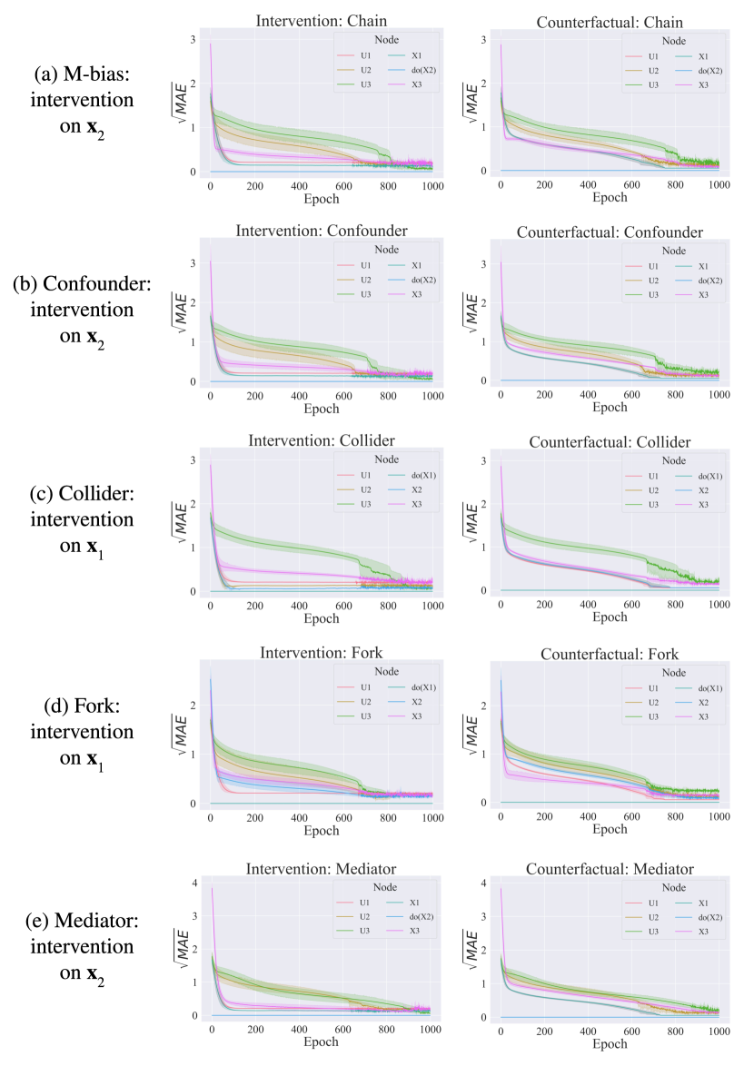
Figure 20: Performance of interventional and counterfactual inference throughout SCM learning process. For each three node causal graph we choose a specific intervention node, if available a node that is neither a root nor leaf node, and track MAE by node.

The experiments in this section display that our method is able to infer correctly associational, interventional, and counterfactual distributions. More specifically, we show how we can (1) learn the parameters of the SCM (structural equations and exogenous distributions) and (2) deploy the error nodes of a fitted PC model in such a way that allows us to manipulate a structural equation to answer causal queries. First, in Figs. 16 and 17, we show the convergence of our predictive coding network while learning the parameters of the SCM for all three and five node causal graphs. In the left column, we can see that our method converges for all graph structures and that we do not overfit the training data. Moreover, we observed that a low free energy does not correspond to a converged model. The MAE continues to decrease, while the energy changes minimally after 50 epochs. The right column shows that the convergence is stable and smooth among all nodes in the causal graph. We show the free energy by node for all exogenous and endogenous variables. Second, in Figs. 18 and 19, we show the causal inference performance of our method by tracking the MAE for associational, interventional, and counterfactual test queries throughout the SCM learning process. We perform interventions on all types of nodes to show that our model is able to correctly infer causal queries on: root nodes with no parents, intermediate nodes with parents and children, and leaf nodes with no children. Note that the left column represents the associational inference error on the exogenous nodes only because during training we are provided with data of the endogenous variables. Third, in Figs. 20 and 21, we plot the MAE metric for test interventions and counterfactuals during the SCM learning process. We choose intervention nodes that are non-trivial by selecting, wherever available, intervention nodes that are neither root nor leaf nodes.

To conclude, in Table 1, we summarize our results and compare our method to state-of-the-art models on all common causal graphs of this work. First, we see that our method consistently outperforms all state-of-the-art methods, on all causal graph structures, for all types of causal queries. Second, we see that a further advantage of our method is that our PC network is as efficient as the underlying SCM that generated the data. Compared to the state-of-the-art methods presented in [Sánchez-Martin et al., 2022, Khemakhem et al., 2021, Karimi et al., 2020], which require thousands of parameters to infer causal distributions, our method only requires as many parameters as the true SCM. More specifically, we only learn the parameters for each of the exogenous distributions plus one parameter for each adjacency weight that connects two nodes in the causal graphs.

Discussion.

Our proposed method does not require more parameters than the number of parameters that define the true structural equations of the SCM. As such, our model is lightweight and simple to train. Having explored various hyperparameters, we found that our model is not prone to overfitting nor does it require hyperparameter tuning or model selection to infer causal distributions. The metrics reported in Table 1 show that our method is consistent with the increasing complexity of DAG structures and able to well capture observational, interventional and counterfactual distributions for all graphs. We experimented with varying Gaussian distribution parameters for the exogenous variables and found that our causal inference approach is robust to arbitrary Gaussians. As such, our method does not require the assumption of standard normally distributed exogenous variables as is the case in some of the related literature [Sánchez-Martin et al., 2022, Saha and Garain, 2022, Chao et al., 2023]. Furthermore, our model is minimal as in being the simplest model that adequately explains the data which is shown by the number of parameters our model architectures require. Therefore, we provide an Occam’s razor like solution [Blumer et al., 1987] for causal inference with linear SCMs. Finally, we do not rely on complex approximators, such as GNN, VAE, gradient boosted regressor or normalizing flow models that require extensive hyperparameter tuning, to learn causal relationships between the observed variables.

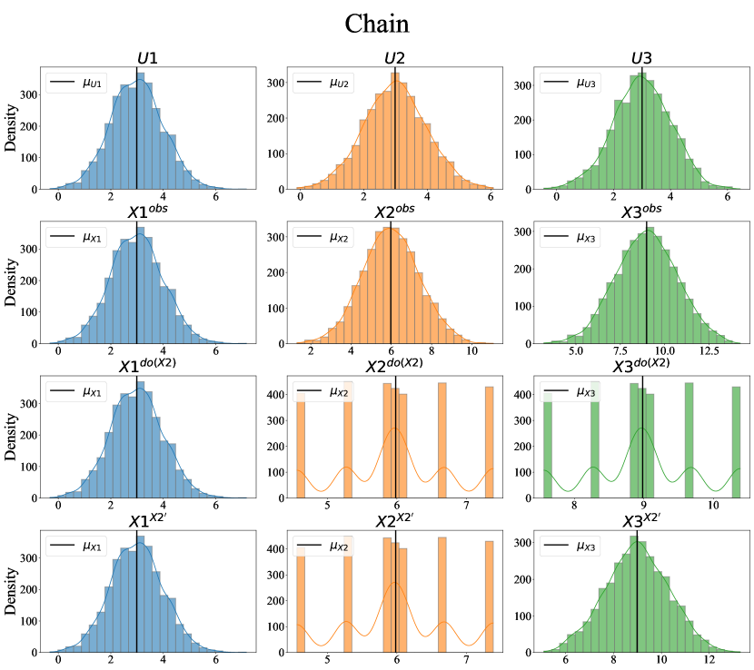
Figure 9: Causal hierarchy of distributions for chain SCM with intervention on $\mathbf{x}_{2}$. First row: Exogenous distribution. Second row: Associational distribution. Third row: Interventional distribution. Last row: Counterfactual distribution.

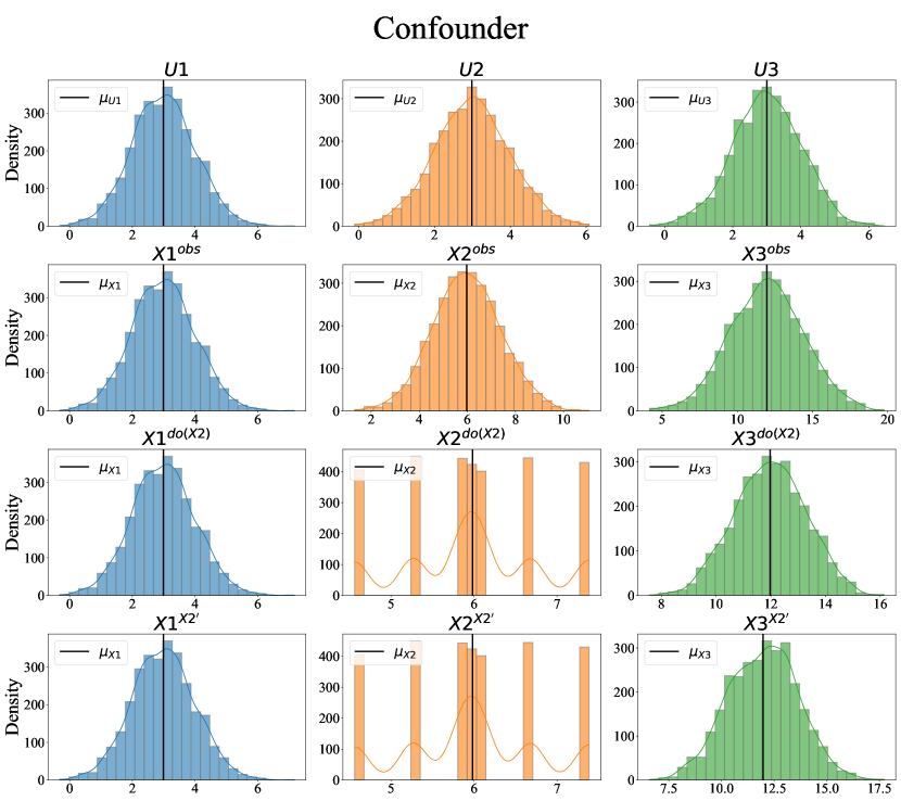
Figure 10: Causal hierarchy of distributions for confounder SCM with intervention on $\mathbf{x}_{2}$. First row: Exogenous distribution. Second row: Associational distribution. Third row: Interventional distribution. Last row: Counterfactual distribution.

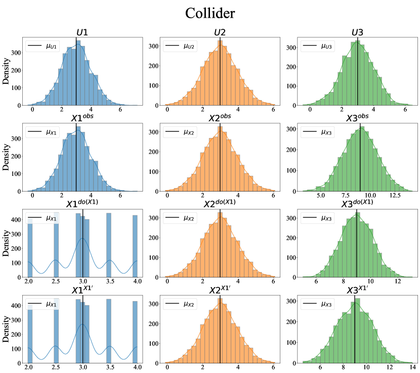
Figure 11: Causal hierarchy of distributions for collider SCM with intervention on $\mathbf{x}_{1}$. First row: Exogenous distribution. Second row: Associational distribution. Third row: Interventional distribution. Last row: Counterfactual distribution.

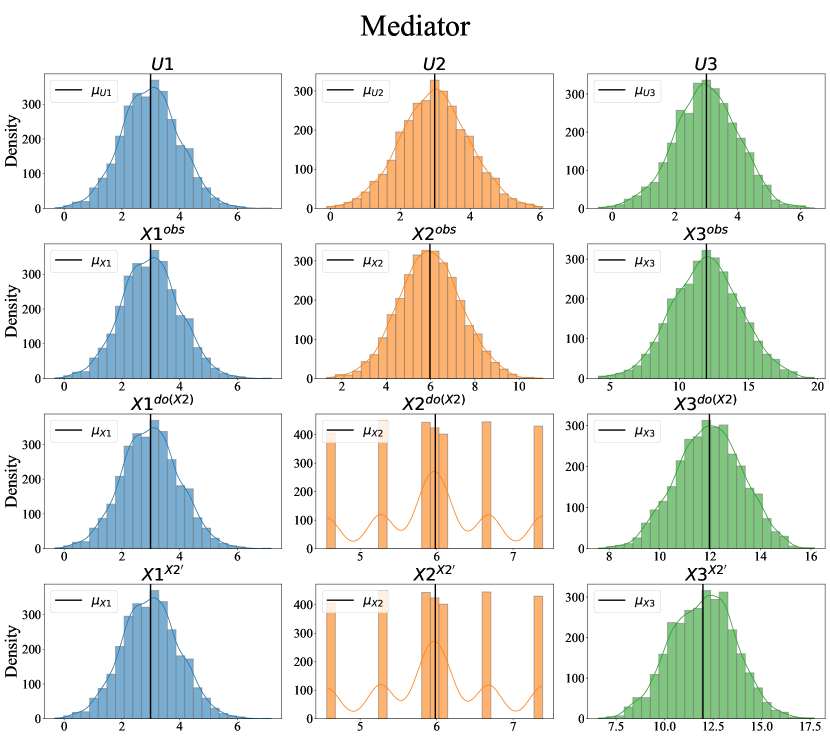
Figure 13: Causal hierarchy of distributions for mediator SCM with intervention on $\mathbf{x}_{2}$. First row: Exogenous distribution. Second row: Associational distribution. Third row: Interventional distribution. Last row: Counterfactual distribution.

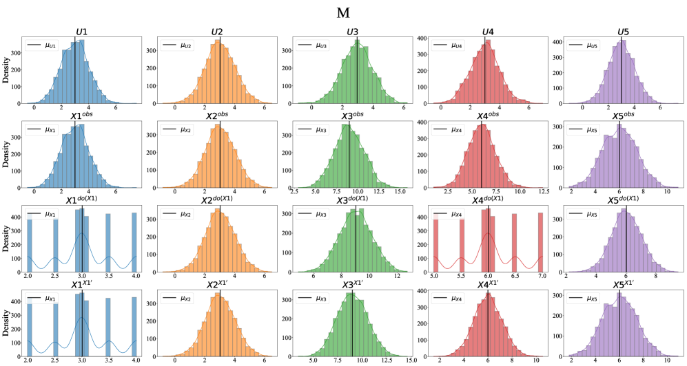
Figure 14: Causal hierarchy of distributions for M-bias SCM with intervention on $\mathbf{x}_{1}$. First row: Exogenous distribution. Second row: Associational distribution. Third row: Interventional distribution. Last row: Counterfactual distribution.

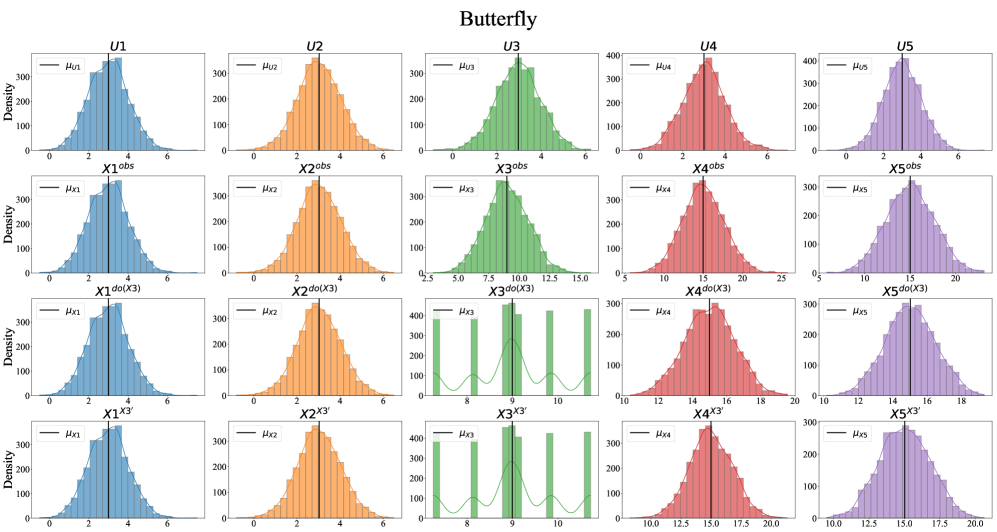
Figure 15: Causal hierarchy of distributions for butterfly bias SCM with intervention on $\mathbf{x}_{3}$. First row: Exogenous distribution. Second row: Associational distribution. Third row: Interventional distribution. Last row: Counterfactual distribution.

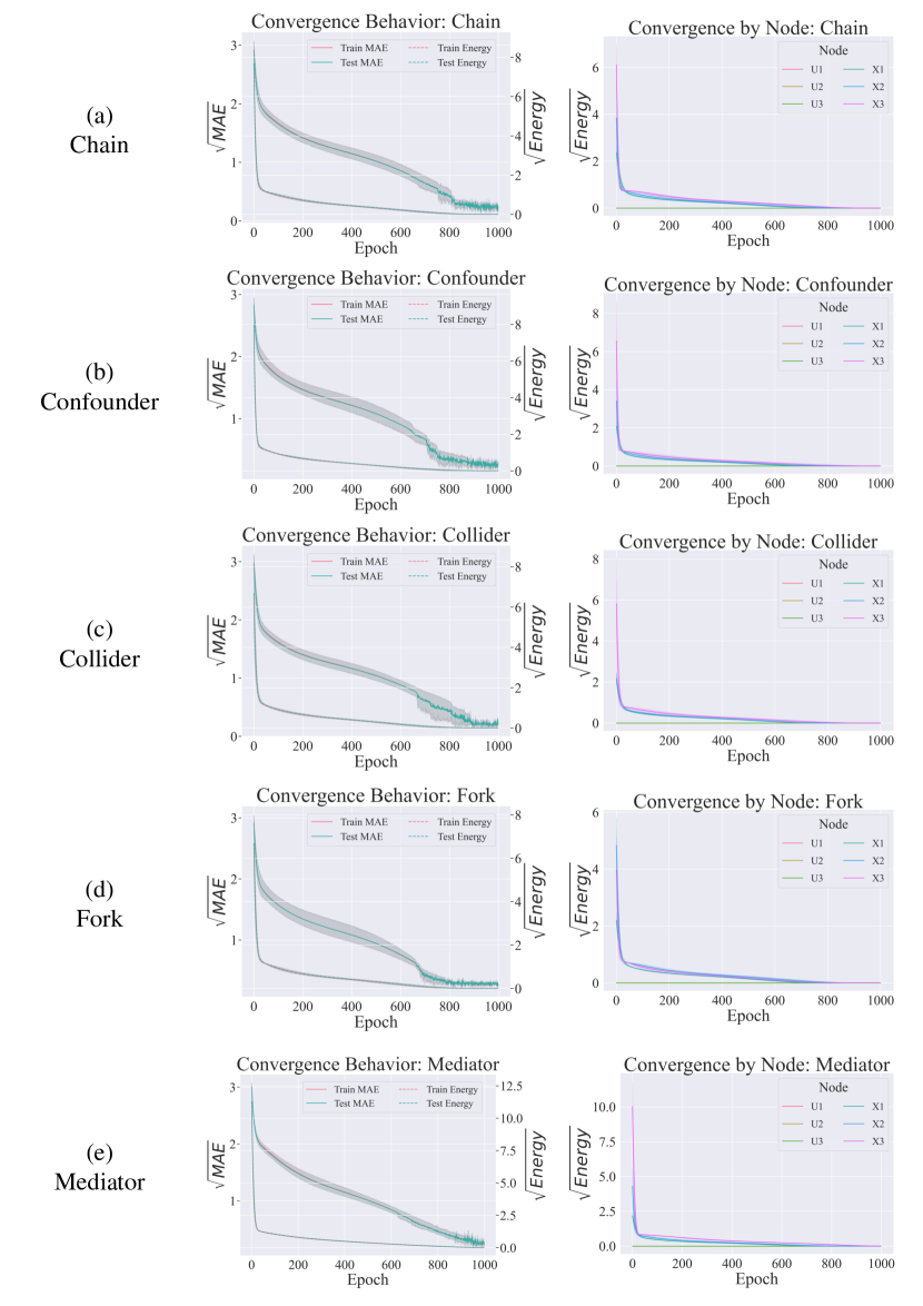
Figure 16: Convergence of energy and MAE by node for causal graphs with three nodes. Left column: Convergence of total train and test MAE in comparison to free energy. Right column: Energy by node.

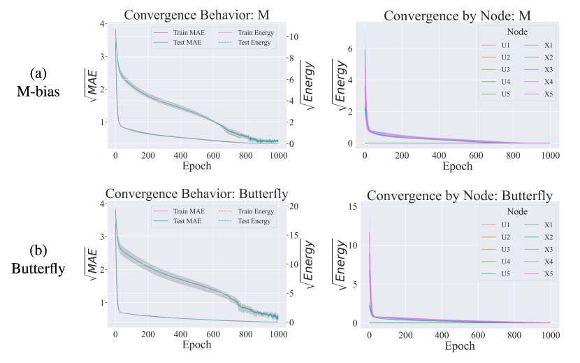
Figure 17: Convergence of energy and MAE by node for causal graphs with five nodes. Left column: Convergence of total train and test MAE in comparison to free energy. Right column: Energy by node.

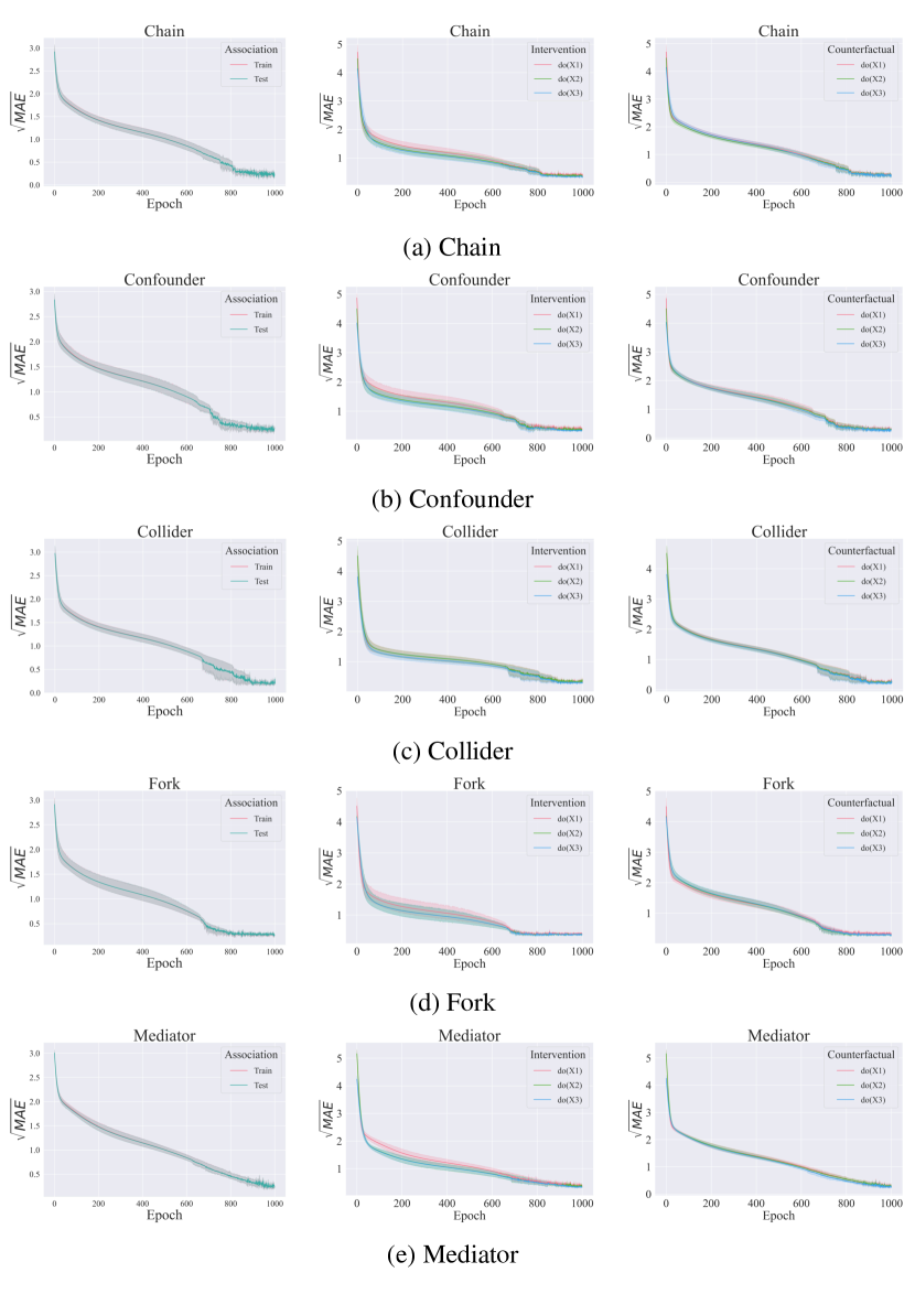
Figure 18: Causal inference performance throughout SCM learning process. We track MAE for all interventions of all three node causal graphs. For association plots (left column) inference is performed on exogenous nodes given factual test data.

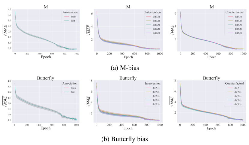
Figure 19: Causal inference performance throughout SCM learning process. We track MAE for all interventions of all five node causal graphs. For association plots (left column) inference is performed on exogenous nodes given factual test data.

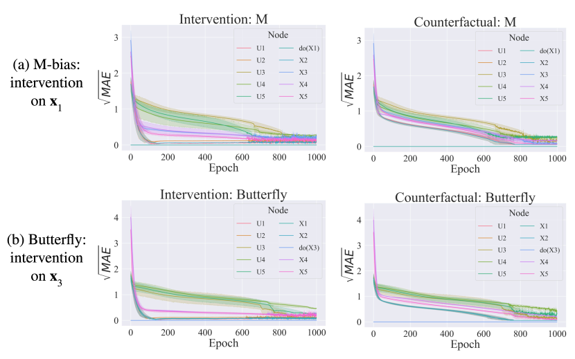
Figure 21: Performance of interventional and counterfactual inference throughout SCM learning process. For each five node causal graph we choose a specific intervention node, if available a node that is neither a root nor leaf node, and track MAE by node.

		Observational	Interventional			Counterfactual
SCM	Model	MMD $\downarrow$	MMD $\downarrow$	MeanE $\downarrow$	StdE $\downarrow$	MSE $\downarrow$	SSE $\downarrow$	Params. # $\downarrow$
chain	Ours	0.01 $\pm$ 0.01	0.04 $\pm$ 0.05	0.21 $\pm$ 0.25	0.00 $\pm$ 0.00	0.68 $\pm$ 0.30	0.49 $\pm$ 0.23	8
	MultiCVAE	7.98$\pm$1.16	62.66$\pm$6.47	75.74$\pm$3.94	40.53$\pm$1.09	57.74$\pm$12.24	25.92$\pm$7.01	7145
	CAREFL	14.81$\pm$0.63	19.70$\pm$0.28	1.29$\pm$0.40	89.53$\pm$1.88	36.58$\pm$5.17	29.78$\pm$4.10	1488
	VACA	4.73$\pm$1.01	14.65$\pm$4.54	8.34$\pm$2.43	19.78$\pm$0.72	98.21$\pm$8.85	6.08$\pm$2.06	2045
confounder	Ours	0.02 $\pm$ 0.02	0.04 $\pm$ 0.04	0.21 $\pm$ 0.19	0.01 $\pm$ 0.01	1.30 $\pm$ 0.15	0.91 $\pm$ 0.11	9
	MultiCVAE	4.35$\pm$0.63	56.68$\pm$3.86	135.05$\pm$5.03	45.62$\pm$1.00	52.40$\pm$11.85	23.11$\pm$3.65	7209
	CAREFL	16.48$\pm$0.72	26.04$\pm$1.03	0.91$\pm$0.38	96.90$\pm$2.56	32.59$\pm$6.41	32.05$\pm$10.56	1488
	VACA	4.48$\pm$1.59	10.94$\pm$6.06	5.43$\pm$1.56	17.85$\pm$0.49	78.80$\pm$14.23	5.34$\pm$1.58	2454
collider	Ours	0.03 $\pm$ 0.03	0.05 $\pm$ 0.04	0.33 $\pm$ 0.33	0.03 $\pm$ 0.01	1.18 $\pm$ 0.18	0.85 $\pm$ 0.14	8
	MultiCVAE	10.41$\pm$1.25	47.12$\pm$10.20	58.73$\pm$3.57	68.06$\pm$3.22	81.63$\pm$15.99	49.35$\pm$7.12	7145
	CAREFL	12.39$\pm$0.73	10.50$\pm$0.14	1.15$\pm$0.31	94.69$\pm$3.53	31.06$\pm$5.18	30.51$\pm$5.13	1488
	VACA	4.13$\pm$2.70	9.79$\pm$6.99	4.96$\pm$3.02	34.51$\pm$0.78	97.74$\pm$21.20	12.53$\pm$2.82	2045
fork	Ours	0.03 $\pm$ 0.01	0.02 $\pm$ 0.02	0.04 $\pm$ 0.03	0.01 $\pm$ 0.00	1.13 $\pm$ 0.09	0.80 $\pm$ 0.06	8
	MultiCVAE	11.28$\pm$1.44	46.91$\pm$10.52	59.04$\pm$4.35	67.76$\pm$3.32	81.16$\pm$15.48	49.10$\pm$7.04	7145
	CAREFL	11.39$\pm$0.65	10.44$\pm$0.47	0.77$\pm$0.25	94.62$\pm$3.68	29.51$\pm$5.34	31.22$\pm$2.88	1488
	VACA	5.26$\pm$3.12	9.19$\pm$7.00	4.67$\pm$2.92	34.41$\pm$0.72	97.62$\pm$23.12	13.97$\pm$3.10	2045
mediator	Ours	0.02 $\pm$ 0.02	0.03 $\pm$ 0.03	0.13 $\pm$ 0.13	0.01 $\pm$ 0.01	1.27 $\pm$ 0.27	0.89 $\pm$ 0.20	9
	MultiCVAE	5.93$\pm$0.88	55.31$\pm$3.57	134.42$\pm$5.23	46.64$\pm$1.50	52.18$\pm$11.70	23.19$\pm$3.89	7209
	CAREFL	13.60$\pm$0.64	26.04$\pm$1.03	0.91$\pm$0.38	96.90$\pm$2.56	34.93$\pm$8.19	36.05$\pm$13.23	1488
	VACA	6.25$\pm$2.06	10.94$\pm$6.06	5.43$\pm$1.56	17.85$\pm$0.49	78.69$\pm$14.21	5.61$\pm$1.70	2454
M-bias	Ours	0.03 $\pm$ 0.01	0.23 $\pm$ 0.15	0.22 $\pm$ 0.14	0.01 $\pm$ 0.00	1.23 $\pm$ 0.13	0.81 $\pm$ 0.09	14
	MultiCVAE	16.20$\pm$2.69	63.95$\pm$7.35	58.02$\pm$1.90	32.36$\pm$2.73	47.15$\pm$10.02	19.55$\pm$4.99	11951
	CAREFL	19.47$\pm$1.63	15.62$\pm$0.74	0.92$\pm$0.23	67.21$\pm$3.04	26.39$\pm$2.63	20.73$\pm$0.58	3080
	VACA	2.50$\pm$0.46	6.60$\pm$1.53	3.35$\pm$0.93	12.53$\pm$0.22	62.26$\pm$4.97	6.53$\pm$2.36	3681
butterfly	Ours	0.10 $\pm$ 0.03	0.27 $\pm$ 0.11	0.43 $\pm$ 0.24	0.02 $\pm$ 0.00	2.84 $\pm$ 0.38	1.88 $\pm$ 0.21	16
	MultiCVAE	16.85$\pm$3.31	83.44$\pm$10.15	139.98$\pm$5.83	79.49$\pm$11.86	55.45$\pm$3.50	24.49$\pm$2.64	12079
	CAREFL	22.03$\pm$2.28	38.93$\pm$1.16	1.23$\pm$0.17	88.59$\pm$3.31	23.52$\pm$3.20	18.14$\pm$1.48	3080
	VACA	4.16$\pm$0.55	6.89$\pm$1.25	3.83$\pm$0.90	8.73$\pm$0.11	57.40$\pm$3.84	4.16$\pm$0.94	4499

Table 1: Comparing our method against state-of-the-art methods for estimating observational, interventional, and counterfactual distributions of various SCM structures. For clarity, all values are multiplied by 100. Mean and standard deviation are reported over five different seeds.

Appendix C Classification Experiments

Here, we provide all the information needed to reproduce the results of the classification experiments provided in the main body of the paper. Furthermore, we also provide a more detailed study on how the results are affected when changing the parameters of the model.

Setup.

The primary focus of our experiments is on the training of fully-connected neural network models with $2000$ neurons on two datasets: MNIST and FashionMNIST. The chosen architecture for the models is a simple fully connected PC graph. For the models, we conducted an exhaustive hyperparameter search. We opted for a grid search approach, examining several combinations of learning rates for the weights and the latent variables, and subsequently training the models for each combination. The chosen learning rates for the weights were $\{0.0001,0.00005,0.00001\}$. As for the latent variables, the learning rates tested were $\{1,0.5\}$, and every batch of $128$ examples was observed for $T\in\{3,5,7\}$ iterations. To optimize the weights of our models, we have used the Adam optimizer; for the value nodes, we have used SGD; as an activation function, ReLU. To conclude, have also tested incremental predictive coding (iPC), a variation of PC that updates the weight parameters at every time step $t$. This method has been shown to improve both the performance and the stability of predictive coding models [Salvatori et al., 2022c]. Training was performed for $20$ epochs for each combination of learning rates in the grid search. It is important to note that training always converged before the 20th epoch, ensuring a stable model for each hyperparameter combination. At every epoch of the training process, we have computed the test accuracy using both interventional queries and conditional queries.

Results.

The results of our experiments showed a clear pattern: regardless of the combination of hyperparameters, interventional queries consistently outperformed conditional queries. This pattern was observed across all models and datasets, suggesting that interventional queries might be a more effective tool for PC graphs. The best results were obtained using a learning rate of the value nodes of $0.5$, and $T=3$. The learning rate of the parameters slightly affected the performance, unless we consider values outside the proposed range. As a learning algorithm, we observe that iPC is indeed more performing and stable, as shown in Figure 22.

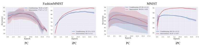
Figure 22: Difference in performance and stability of iPC and PC on classification tasks.

Appendix D Robustness Experiments

Recent work has shown that available deep-learning-based methods fail to obtain sufficient performance on counterfactual queries under specific circumstances, and proposed novel techniques to overcome this shortcoming [De Brouwer, 2022]. Here, we show that predictive coding achieves the same state-of-the-art results, while requiring a simpler architecture with no ad hoc training techniques. To do so, we test PC graphs on the colored-MNIST dataset introduced in [De Brouwer, 2022]. The dataset consists of tuples $(\mathbf{x},\mathbf{u}_{z},\mathcal{T},\mathbf{y},\mathcal{T}^{\prime},\mathbf{y}^{\prime})$, where $\mathbf{x}$ is the original MNIST image, $\mathcal{T}$ is the assigned treatment, $\mathbf{u}_{z}$ is a hidden exogenous random variable that determines the color of the observed outcome image $\mathbf{y}$, and $\mathbf{y}^{\prime}$ is the counterfactual response obtained when applying the alternative treatment $\mathcal{T}^{\prime}$.

Setup.

To replicate the experiment, we have used a PC graph with a structure that is equivalent to the $4$-nodes SCM used in the original work, and trained it with Algorithm 1. We used nodes with the ground truth number of dimensions (i.e., $784$, $1$, and $784$ respectively) to represent the observed variables $\mathbf{x}$, $\mathcal{T}$, and $\mathbf{y}$. Instead, we left the dimension of the remaining hidden node $h$ as a hyperparameter $d_{h}$ as the value $\mathbf{u}_{z}$ is never observed by the model. The edges between the nodes in the PC graph represent feedforward networks. Figure 5 summarizes the architecture used. We experimented with different depths, widths, and activation functions, without experiencing any unexpected results (e.g., deeper and wider networks would have slightly better performance). The architecture can be seen as an encoder-decoder structure. The nodes $\mathbf{x}$, $\mathcal{T}$, and $\mathbf{u}_{z}$ are encoded using respectively $3$, $1$, and $1$ fully connected layers with a hidden dimensions of $1024$ and tanh as activation function. Then, the embedding is decoded into $\mathbf{y}$ using $3$ other fully connected layers with the same hidden dimension of $1024$. The experiment was conducted as follows:

• During training, we fix the nodes $\mathbf{x}$, $\mathcal{T}$, and $\mathbf{y}$ to the corresponding observed variables and we initialize $h$ to $0$. We train for $128$ epochs with a batch size of $256$. We train using iPC and $T=16$. We set the nodes learning rate to $\gamma=0.005$ and the weights learning rate to $\alpha=0.00005$. We use the SGD optimizer for the nodes and the Adamw optimizer for the weights. Consequently, the model has never direct access to any of $\mathbf{u}_{z}$, $\mathcal{T}^{\prime}$, or $\mathbf{y}^{\prime}$.

• The inference process is divided in two phases. Firstly, we repeat the same procedure as above, while setting $\alpha=0.0$, so that the weights of the model are not changed. This allows the network to adapt to the provided $\mathbf{y}$ by storing its extra information (i.e., the color, in this instance) in the hidden node $\mathbf{u}_{z}$. Secondly, for each sample in a batch, after $T=16$ steps, we replace $\mathcal{T}$ with $\mathcal{T}^{\prime}$ to compute the counterfactual $\mathbf{y}^{\prime}$ and compare it with the ground truth image. To obtain $\mathbf{y}^{\prime}$, we simply forward through the network the information stored in the nodes $\mathbf{x}$, $\mathcal{T}$, and $\mathbf{u}_{z}$ during the first phase. To produce the digits in Fig. 5, we fixed the node $\mathcal{T}$ to each angle $\in\{0^{\circ},10^{\circ},20^{\circ},30^{\circ},40^{\circ}\}$. Furthermore, our model is able to produce counterfactual not only by modifying the rotation $\mathcal{T}$, but also the color encoded by $\mathbf{u}_{z}$. To show this, we take the value of the node $\mathbf{u}_{z}$ computed for the a sample and use it to generate all the remaining $\mathbf{y}^{\prime}$ in the batch.

Results.

We obtain results comparable with the ones in [De Brouwer, 2022]. Our method has the advantage of using a straightforward multi-layer perceptron architecture trained with an unmodified version of the predictive coding learning algorithm. This shows the capability and versatility of predictive coding to work in various tasks in which other deep-learning techniques tend to fail, such as Diff-SCM [Sanchez and Tsaftaris, 2022b], Deep-SCM [Pawlowski et al., 2020b], and Deep-ITE [Shalit et al., 2017]. Figure 5 in the main body shows a magnified example of counterfactual reconstructions that demonstrate that our method is robust with respect to interventions on either rotation or color. Compared to [De Brouwer, 2022], we are able to generalize to rotations of $40^{\circ}$, even if this introduces some noise in the generated output. Furthermore, contrary to the model presented in [De Brouwer, 2022], our architecture is robust with respect to the choice of the hyperparameter linked to $u_{z}$ and does not necessitate to perform a hyperparameter sweep to find the right value.

Appendix E Structure Learning

E.1 Experiments on Random Graphs

In this section, we show results on the convergence behavior of structure learning with a PC graph to understand the relationship between variational free energy and the approximation error of the weighted adjacency matrix. Furthermore, we describe in detail the metrics used to evaluate the estimated weighted adjacency matrix as well as accuracy metrics for assessing the learned relationships and directions of the adjacency matrix. We also provide all the details on the model and training parameters used to reproduce our causal discovery experiments. Finally, we compare our method to causal discovery baselines for various types of complexities of random graphs.

Setup.

Our causal structure learning method only requires observational data as input. The two types of random graphs that we consider for our experiments are (1) Erdős-Rényi (ER) with either 1 or 2 expected edges per node, denoted as ER1 and ER2, and (2) scale-free (SF) graphs with either 2 or 4 expected edges per node, denoted as SF2 and SF4, respectively. We use graphs with $N\in\{10,15,20\}$ nodes and generate datasets with $2000$ samples. These two graph types are selected to demonstrate the versatility and robustness of our method in handling various graph structures.

We generate synthetic data by first sampling a binary adjacency matrix, $\mathbf{A}$, for a DAG. Next, we place uniformly random edge weights onto the binary adjacency matrix, to obtain a weighted adjacency matrix, $\mathbf{W}$. Finally, we sample observational data based on a set of linear structural equations with additive Gaussian noise, $\mathbf{u}\sim\mathcal{N}(\mathbf{0},\mathbf{I}_{N})$, such that

$$\mathbf{x}=\mathbf{W}^{T}\mathbf{x}+\mathbf{u}\in\mathbb{R}^{N}.$$

To fit the PC model to the observational data, we use the stochastic gradient descent (SGD) optimizer for the node values with a learning rate of $\gamma=1e-4$ and $T=16$. For the weights, we use the Adamw optimizer with a learning rate of $\alpha=5e-3$. We enforce two penalties onto our learning algorithm. First, a DAG penalty to ensure that the discovered graph is acyclic and directed, as proposed in [Zheng et al., 2018]. Second, an L1 penalty that encourages the PC network to find a causal structure that is sparse. We add both penalties into the predictive coding objective. The penalties are each weighted by $\lambda_{L1}=5e-6$ and $\lambda_{DAG}=200$, for L1 and DAG penalty, respectively.

Structure learning metrics

Here, we describe the metrics used to evaluate the performance for estimating causal graph structures in the experiments of Section 4. First, for the weighted adjacency matrix of a DAG with $N$ nodes, we report the mean absolute error (MAE) between the true, $\mathbf{W}$, and the estimated, $\widehat{\mathbf{W}}$, weighted adjacency matrix as the average of the absolute differences between corresponding entries in the two matrices:

$$\text{MAE}(\mathbf{W},\widehat{\mathbf{W}})=\frac{1}{N^{2}}\sum_{i=1}^{N}\sum_{j=1}^{N}|\mathbf{W}_{ij}-\widehat{\mathbf{W}}_{ij}|.$$ (16)

Second, to evaluate the correctness of the learned edge directions and the adjacency relationships in the causal graph, we report metrics on the estimated binary adjacency matrix, $\widehat{\mathbf{A}}$, that is obtained via thresholding as follows:

$$\widehat{\mathbf{A}}_{ij}=\begin{cases}1&\text{if }\widehat{\mathbf{W}}_{ij}>\omega\\ 0&\text{otherwise.}\end{cases}$$

We use the same data as proposed in [Zheng et al., 2018], and we follow their procedure and use $\omega=0.3$ in all experiments. We report the following graph metrics: (i) F-score (F1), (ii) structural Hamming distance (SHD), (iii) false discovery rate (FDR), (iv) true positive rate (TPR), (iv) false positive rate (FPR), and (v) number of directed edges discovered (NNZ). Each metric is computed between the true adjacency matrix, $\mathbf{A}$, and the estimated adjacency matrix, $\widehat{\mathbf{A}}$. To compute each metric, we first need the following quantities:

• true positive (TP): a discovered edge, with correct direction,

• reverse (R): a discovered edge, with incorrect direction,

• false positive (FP): a discovered edge, not present in $\mathbf{A}$,

• true negative (TN): a non-discovered edge, not present in $\mathbf{A}$,

• false negative (FN): a non-discovered edge, present in $\mathbf{A}$,

• missing (M): a non-discovered edge, present in $\mathbf{A}$.

Based on these quantities, each metric is computed as follows:

• $\text{F1}=\frac{2\text{TP}}{2\text{TP}+\text{FP}+\text{FN}}$,

• $\text{SHD}=\text{R}+\text{M}+\text{FP}=\sum_{i=1}^{N}\sum_{j=1}^{N}|\mathbf{A}_{ij}-\widehat{\mathbf{A}}_{ij}|$,

• $\text{FDR}=\frac{\text{FP}+\text{R}}{\text{FP}+\text{TP}}$,

• $\text{FPR}=\frac{\text{FP}+\text{R}}{\text{FP}+\text{TN}}$,

• $\text{TPR}=\frac{\text{TP}}{\text{TP}+\text{FN}}$,

• $\text{NNZ}=\text{TP}+\text{FP}$.

Results.

First, we show results on learning the causal structure for the two most difficult graphs of our experiments, namely, ER2 and SF4 graphs, each with $N=20$. We see that PC graphs are able to learn good approximations of the ground truth weighted adjacency matrix of complex random graphs. This is depicted in the left columns of Figs. 23 and 24, respectively. The right columns in Figs. 23 and 24 shows how the MAE decreases as the predictive coding objective converges. In all cases, we observe that while the energy converges early on, the causal discovery performance (MAE) keeps improving. Second, in Table 2, we compare our method against established and recent causal discovery algorithms. In contrast to the baselines, our method consistently exhibits a good performance across various graph structures and does not deteriorate strongly for graphs of varying complexity by maintaining its causal structure learning abilities despite irregular node degree distributions and an increasing number of edges and nodes. This is reflected in the high accuracy metrics (F1) and low structural hamming distance (SHD) obtained with our method. From our experiments, we observed that our method performs very well on scale-free graphs different to most of the benchmarks, which struggle on such random graphs. To conclude, the causal structure learning experiments conducted demonstrate that our method can learn arbitrary DAG structures of varying characteristics and levels of complexity. The complexity is determined by factors such as the number of nodes in the graph and the degree distribution of each node. Furthermore, our method demonstrates a robust performance even in the face of challenges such as increasingly uneven degree distributions and growing node cardinality. This distinguishes our approach from the baseline methods, thereby further highlighting the effectiveness of our predictive coding framework for causal structure learning.

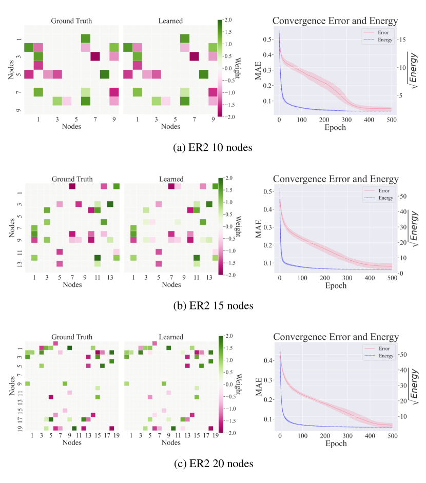
Figure 23: Learned structures and convergence behavior (energy vs. MAE) for ER2 graphs of various complexity.

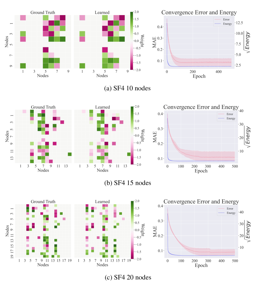
Figure 24: Learned structures and convergence behavior (energy vs. MAE) for SF4 graphs of various complexity.

model	$N$	graph	FDR $\downarrow$	TPR $\uparrow$	FPR $\downarrow$	SHD $\uparrow$	NNZ -	F1 $\uparrow$
Ours			0.11 $\pm$ 0.11	0.92 $\pm$ 0.08	0.03 $\pm$ 0.04	1.40 $\pm$ 1.34	10.40 $\pm$ 1.14	0.90 $\pm$ 0.09
GES			0.22 $\pm$ 0.08	0.88 $\pm$ 0.11	0.07 $\pm$ 0.03	3.00 $\pm$ 1.41	11.20 $\pm$ 0.45	0.68 $\pm$ 0.09
PC	10	ER1	0.13 $\pm$ 0.04	0.82 $\pm$ 0.04	0.03 $\pm$ 0.01	2.20 $\pm$ 0.45	9.40 $\pm$ 0.55	0.77 $\pm$ 0.03
ICALiNGAM			0.25 $\pm$ 0.15	0.86 $\pm$ 0.11	0.09 $\pm$ 0.05	3.20 $\pm$ 2.05	11.60 $\pm$ 1.14	0.80 $\pm$ 0.13
NOTEARS			0.00 $\pm$ 0.00	1.00 $\pm$ 0.00	0.00 $\pm$ 0.00	0.00 $\pm$ 0.00	10.00 $\pm$ 0.00	1.00 $\pm$ 0.00
Ours			0.04 $\pm$ 0.05	0.91 $\pm$ 0.09	0.03 $\pm$ 0.04	2.40 $\pm$ 2.27	19.00 $\pm$ 1.63	0.93 $\pm$ 0.06
GES			0.86 $\pm$ 0.03	0.26 $\pm$ 0.05	1.30 $\pm$ 0.02	33.60 $\pm$ 0.55	37.60 $\pm$ 1.14	0.17 $\pm$ 0.03
PC	10	ER2	0.47 $\pm$ 0.09	0.45 $\pm$ 0.08	0.32 $\pm$ 0.06	13.20 $\pm$ 1.48	17.00 $\pm$ 0.71	0.47 $\pm$ 0.08
ICALiNGAM			0.31 $\pm$ 0.14	0.74 $\pm$ 0.12	0.27 $\pm$ 0.13	9.20 $\pm$ 4.76	21.60 $\pm$ 1.14	0.71 $\pm$ 0.13
NOTEARS			0.07 $\pm$ 0.03	0.85 $\pm$ 0.09	0.05 $\pm$ 0.02	3.00 $\pm$ 1.87	18.20 $\pm$ 1.79	0.89 $\pm$ 0.06
Ours			0.06 $\pm$ 0.08	0.97 $\pm$ 0.04	0.01 $\pm$ 0.02	1.20 $\pm$ 1.79	15.60 $\pm$ 0.89	0.87 $\pm$ 0.07
GES			0.22 $\pm$ 0.14	0.83 $\pm$ 0.10	0.04 $\pm$ 0.03	5.00 $\pm$ 3.00	16.00 $\pm$ 1.00	0.80 $\pm$ 0.12
PC	15	ER1	0.16 $\pm$ 0.05	0.85 $\pm$ 0.03	0.03 $\pm$ 0.01	3.40 $\pm$ 0.89	15.20 $\pm$ 0.45	0.78 $\pm$ 0.03
ICALiNGAM			0.30 $\pm$ 0.06	0.77 $\pm$ 0.09	0.06 $\pm$ 0.01	5.40 $\pm$ 1.14	16.60 $\pm$ 1.52	0.73 $\pm$ 0.07
NOTEARS			0.00 $\pm$ 0.00	1.00 $\pm$ 0.00	0.00 $\pm$ 0.00	0.00 $\pm$ 0.00	15.00 $\pm$ 0.00	1.00 $\pm$ 0.00
Ours			0.18 $\pm$ 0.01	0.85 $\pm$ 0.03	0.07 $\pm$ 0.01	10.20 $\pm$ 0.45	31.00 $\pm$ 1.41	0.83 $\pm$ 0.01
GES			0.56 $\pm$ 0.08	0.77 $\pm$ 0.07	0.40 $\pm$ 0.10	31.60 $\pm$ 7.70	52.80 $\pm$ 5.72	0.54 $\pm$ 0.08
PC	15	ER2	0.62 $\pm$ 0.07	0.37 $\pm$ 0.06	0.24 $\pm$ 0.03	33.40 $\pm$ 3.05	28.80 $\pm$ 1.48	0.37 $\pm$ 0.07
ICALiNGAM			0.38 $\pm$ 0.08	0.75 $\pm$ 0.08	0.18 $\pm$ 0.04	17.60 $\pm$ 3.65	36.20 $\pm$ 2.49	0.68 $\pm$ 0.07
NOTEARS			0.10 $\pm$ 0.03	0.91 $\pm$ 0.04	0.04 $\pm$ 0.01	5.80 $\pm$ 1.64	30.20 $\pm$ 1.30	0.90 $\pm$ 0.03
Ours			0.25 $\pm$ 0.04	0.99 $\pm$ 0.02	0.04 $\pm$ 0.01	6.80 $\pm$ 1.48	26.60 $\pm$ 1.14	0.80 $\pm$ 0.04
GES			0.43 $\pm$ 0.12	0.74 $\pm$ 0.13	0.07 $\pm$ 0.02	14.90 $\pm$ 6.47	26.30 $\pm$ 1.95	0.65 $\pm$ 0.13
PC	20	ER1	0.43 $\pm$ 0.08	0.61 $\pm$ 0.07	0.06 $\pm$ 0.01	13.80 $\pm$ 1.92	21.60 $\pm$ 1.14	0.54 $\pm$ 0.07
ICALiNGAM			0.47 $\pm$ 0.05	0.72 $\pm$ 0.06	0.08 $\pm$ 0.01	14.60 $\pm$ 2.19	27.20 $\pm$ 1.92	0.61 $\pm$ 0.05
NOTEARS			0.23 $\pm$ 0.08	0.79 $\pm$ 0.07	0.03 $\pm$ 0.01	8.80 $\pm$ 2.86	20.60 $\pm$ 0.55	0.78 $\pm$ 0.07
Ours			0.15 $\pm$ 0.05	0.91 $\pm$ 0.02	0.04 $\pm$ 0.02	9.40 $\pm$ 1.95	42.80 $\pm$ 2.59	0.88 $\pm$ 0.03
GES			0.70 $\pm$ 0.07	0.64 $\pm$ 0.11	0.42 $\pm$ 0.10	65.80 $\pm$ 13.57	88.80 $\pm$ 11.90	0.40 $\pm$ 0.09
PC	20	ER2	0.65 $\pm$ 0.04	0.37 $\pm$ 0.06	0.18 $\pm$ 0.01	44.00 $\pm$ 1.41	41.80 $\pm$ 2.39	0.36 $\pm$ 0.05
ICALINGAM			0.34 $\pm$ 0.10	0.80 $\pm$ 0.06	0.11 $\pm$ 0.04	19.60 $\pm$ 6.47	49.20 $\pm$ 4.21	0.72 $\pm$ 0.08
NOTEARS			0.00 $\pm$ 0.00	0.96 $\pm$ 0.01	0.00 $\pm$ 0.00	1.60 $\pm$ 0.55	38.40 $\pm$ 0.55	0.98 $\pm$ 0.01
Ours			0.03 $\pm$ 0.09	0.99 $\pm$ 0.04	0.02 $\pm$ 0.07	0.70 $\pm$ 2.21	17.40 $\pm$ 1.26	0.98 $\pm$ 0.07
GES			0.39 $\pm$ 0.02	0.89 $\pm$ 0.03	0.35 $\pm$ 0.05	9.80 $\pm$ 1.30	25.00 $\pm$ 1.73	0.69 $\pm$ 0.02
PC	10	SF2	0.24 $\pm$ 0.03	0.69 $\pm$ 0.03	0.14 $\pm$ 0.02	7.40 $\pm$ 0.55	15.60 $\pm$ 0.55	0.72 $\pm$ 0.02
ICALiNGAM			0.40 $\pm$ 0.09	0.79 $\pm$ 0.07	0.33 $\pm$ 0.09	10.80 $\pm$ 2.77	22.60 $\pm$ 1.67	0.68 $\pm$ 0.08
NOTEARS			0.00 $\pm$ 0.00	1.00 $\pm$ 0.00	0.00 $\pm$ 0.00	0.00 $\pm$ 0.00	17.00 $\pm$ 0.00	1.00 $\pm$ 0.00
Ours			0.08 $\pm$ 0.08	0.94 $\pm$ 0.06	0.17 $\pm$ 0.19	3.50 $\pm$ 3.78	30.80 $\pm$ 1.87	0.93 $\pm$ 0.07
GES			0.60 $\pm$ 0.05	0.56 $\pm$ 0.07	1.69 $\pm$ 0.12	27.00 $\pm$ 2.35	42.20 $\pm$ 0.45	0.44 $\pm$ 0.05
PC	10	SF4	0.18 $\pm$ 0.08	0.59 $\pm$ 0.06	0.25 $\pm$ 0.12	14.60 $\pm$ 2.41	21.40 $\pm$ 1.52	0.68 $\pm$ 0.06
ICALiNGAM			0.21 $\pm$ 0.06	0.83 $\pm$ 0.05	0.45 $\pm$ 0.15	9.40 $\pm$ 3.21	31.80 $\pm$ 1.64	0.81 $\pm$ 0.06
NOTEARS			0.03 $\pm$ 0.05	0.83 $\pm$ 0.09	0.05 $\pm$ 0.07	5.40 $\pm$ 3.29	25.80 $\pm$ 1.64	0.89 $\pm$ 0.07
Ours			0.02 $\pm$ 0.02	0.98 $\pm$ 0.02	0.01 $\pm$ 0.01	0.60 $\pm$ 0.55	27.00 $\pm$ 0.00	0.98 $\pm$ 0.02
GES			0.27 $\pm$ 0.02	0.99 $\pm$ 0.02	0.13 $\pm$ 0.01	10.00 $\pm$ 1.00	36.80 $\pm$ 0.84	0.79 $\pm$ 0.01
PC	15	SF2	0.15 $\pm$ 0.08	0.76 $\pm$ 0.03	0.05 $\pm$ 0.03	9.40 $\pm$ 2.70	24.00 $\pm$ 1.41	0.77 $\pm$ 0.04
ICALiNGAM			0.36 $\pm$ 0.11	0.87 $\pm$ 0.07	0.17 $\pm$ 0.07	15.20 $\pm$ 7.26	37.20 $\pm$ 3.83	0.74 $\pm$ 0.10
NOTEARS			0.00 $\pm$ 0.00	1.00 $\pm$ 0.00	0.00 $\pm$ 0.00	0.00 $\pm$ 0.00	27.00 $\pm$ 0.00	1.00 $\pm$ 0.00
Ours			0.10 $\pm$ 0.06	0.94 $\pm$ 0.05	0.09 $\pm$ 0.06	7.20 $\pm$ 4.55	52.20 $\pm$ 1.79	0.92 $\pm$ 0.05
GES			0.47 $\pm$ 0.09	0.82 $\pm$ 0.10	0.67 $\pm$ 0.16	39.40 $\pm$ 11.04	77.60 $\pm$ 4.39	0.62 $\pm$ 0.09
PC	15	SF4	0.52 $\pm$ 0.06	0.29 $\pm$ 0.04	0.28 $\pm$ 0.03	45.40 $\pm$ 2.51	30.00 $\pm$ 0.71	0.36 $\pm$ 0.05
ICALiNGAM			0.44 $\pm$ 0.09	0.69 $\pm$ 0.09	0.50 $\pm$ 0.11	36.40 $\pm$ 7.83	62.00 $\pm$ 3.39	0.62 $\pm$ 0.09
NOTEARS			0.09 $\pm$ 0.00	0.85 $\pm$ 0.02	0.07 $\pm$ 0.00	10.40 $\pm$ 0.89	46.60 $\pm$ 0.89	0.88 $\pm$ 0.01
Ours			0.10 $\pm$ 0.14	0.96 $\pm$ 0.05	0.03 $\pm$ 0.04	5.40 $\pm$ 7.40	40.20 $\pm$ 4.38	0.93 $\pm$ 0.10
GES			0.30 $\pm$ 0.12	0.96 $\pm$ 0.02	0.10 $\pm$ 0.05	16.00 $\pm$ 7.28	51.20 $\pm$ 6.98	0.77 $\pm$ 0.08
PC	20	SF2	0.26 $\pm$ 0.07	0.70 $\pm$ 0.06	0.06 $\pm$ 0.02	17.80 $\pm$ 4.38	34.80 $\pm$ 1.48	0.68 $\pm$ 0.06
ICALiNGAM			0.34 $\pm$ 0.17	0.87 $\pm$ 0.06	0.12 $\pm$ 0.08	19.80 $\pm$ 13.01	50.80 $\pm$ 9.88	0.75 $\pm$ 0.13
NOTEARS			0.00 $\pm$ 0.00	1.00 $\pm$ 0.00	0.00 $\pm$ 0.00	0.00 $\pm$ 0.00	37.00 $\pm$ 0.00	1.00 $\pm$ 0.00
Ours			0.06 $\pm$ 0.05	0.98 $\pm$ 0.03	0.04 $\pm$ 0.03	5.60 $\pm$ 5.50	73.00 $\pm$ 1.73	0.96 $\pm$ 0.04
GES			0.28 $\pm$ 0.03	0.94 $\pm$ 0.04	0.21 $\pm$ 0.02	26.60 $\pm$ 3.13	91.40 $\pm$ 1.52	0.79 $\pm$ 0.03
PC	20	SF4	0.38 $\pm$ 0.04	0.34 $\pm$ 0.02	0.12 $\pm$ 0.01	54.60 $\pm$ 2.70	38.80 $\pm$ 1.30	0.44 $\pm$ 0.03
ICALiNGAM			0.37 $\pm$ 0.13	0.73 $\pm$ 0.05	0.27 $\pm$ 0.13	45.20 $\pm$ 17.25	83.40 $\pm$ 12.46	0.67 $\pm$ 0.10
NOTEARS			0.18 $\pm$ 0.01	0.81 $\pm$ 0.02	0.10 $\pm$ 0.01	22.80 $\pm$ 1.64	69.40 $\pm$ 0.55	0.82 $\pm$ 0.02

Table 2: Comparison of our method against different causal discovery baselines on various accuracy metrics for ER and SF graphs of increasing complexity and number of nodes $N$.

E.2 Classification

In the main body of this work, we showed that pruning unnecessary connections in a complete graph results in a hierarchical structure with improved performance. In this section, we provide further details to reproduce our results.

The classification experiments are performed on the MNIST, FashionMNIST, and 2-MNIST datasets. The latter is obtained by pairing the image $\hat{\mathbf{x}}$ in each sample $(\hat{\mathbf{x}},\hat{\mathbf{y}})$ of the MNIST dataset with a new digit image $\hat{\mathbf{x}}^{\prime}$ sampled uniformly from the dataset (while maintaining the train and test splitting intact). Thus, a data point of the 2-MNIST dataset consists of the tuple $(\hat{\mathbf{x}},\hat{\mathbf{x}}^{\prime},\hat{\mathbf{y}})$.

We consider a predictive coding graph with 6 nodes, one of dimension $784$ (input dimension), one of dimension $10$ (output dimension), and 4 hidden nodes of dimension $d$. In the case of 2-MNIST, we have two nodes of dimension 784, and only three of dimension $d$. The results reported in this work were obtained with $d=128$. During training, we used a batch size of $512$ and $T=32$. To start from a complete graph, as the one defined in Section 3, we define a fully connected layer $f_{i,j}$, with $gelu$ activation function, going from node $i$ to node $j$ for each ordered pair of nodes $(i,j)$. The output of each layer $f_{i,j}$ is then multiplied by a scaling factor $a_{i,j}$ that determines the strength of the connection from node $i$ to node $j$. Together, the factors $a_{i,j}$ determine the adjacency matrix $A$. To enforce sparse connectivity and prune unnecessary edges, we add to the matrix $A$ the $L1$ regularizer $l(A)$. Consequently, the loss function to optimize becomes $\mathcal{L}=F+\omega\cdot l(A)$, where $\omega$ is a weighting factor.

To overcome this, we propose two different methods:

1. force an acyclic structure, by adding to the loss function the regulariser $h(A)=tr(exp(A\times A))$ introduced in [Zheng et al., 2018]. We weight $h(A)$ by a scalar $\eta$.

2. force a connection between input nodes and output nodes, by introducing negative samples in the training dataset: with probability $p_{ns}$ we sample randomly a new label $\hat{y}_{ns}$. We modify the energy function:

   $$\hat{F}=\textstyle\sum_{i\neq i_{\mathbf{y}}}\|\mathbf{x}_{i}-\bm{\mu}_{i}\|^{2}+(\|\mathbf{x}_{i_{y}}-\mu_{i_{y}}\|^{2}-k)^{2},$$ (17)

   where $i_{y}$ is the index of the node fixed to $\hat{\mathbf{y}}$ and $k$ the new energy target. We set $k=0$ for positive samples and $k>0$ for negative samples. With negative samples, the output node cannot simply learn to predict itself, as the energy would be non-zero for negative samples, for which the energy target is $k>0$.

Discussion Both methods produce hierarchical structures that achieve a better performance than the original complete graph. Method (1) has the disadvantage of introducing an inductive bias in the architecture by completely removing loops and requiring a complex balance between the $\omega$ and $\eta$ parameters, as they affect each other. On the other hand, method (2), despite overcoming these issues, seems more brittle with respect of the choice of hyperparameters and produces a smaller variety of networks. The value of $\omega$ determines the overall network structure. For method (1), we observed a wide range of possible output structures (e.g., using zero or multiple hidden-nodes, in parallel or in sequence, with and with-out skip connections) depending on the chosen $\omega$. The best accuracy, however, was always achieved with a structure equivalent to a hierarchical neural network with two fully connected layers as shown in Figure 6. For method (2), instead, the only non-degenerate possibilities were either a complete graph (for low $\omega$ values), the optimal 2-layer network, or a network with no edges (for high $\omega$ values). A possible future research direction could be aiming at combining the two methods to overcome their respective limitations. Table 3 reports the best hyperparameters for each method and dataset.

Dataset	Method	$\gamma$	$\alpha$	$\beta$	$\omega$	$\eta$	$p_{ns}$
MNIST	DAG	$0.5$	$4e-05$	$2e-05$	$8e-$4	$40.0$	-
Fashion-MNIST	DAG	$0.3$	$3e-05$	$5e-05$	$1e-3$	$20.0$	-
2-MNIST	DAG	$0.5$	$4e-05$	$2e-05$	$8e-4$	$40.0$	-
MNIST	NS	$0.8$	$1e-04$	$8e-05$	$0.05$	-	$0.1$
Fashion-MNIST	NS	$0.5$	$1e-04$	$8e-05$	$0.05$	-	$0.2$
2-MNIST	NS	$0.8$	$1e-04$	$8e-05$	$0.05$	-	$0.1$

Table 3: Hyperparameters used to obtain the results reported in Fig. 6. DAG (directed acyclic graphs) refers to method (1), while NS (negative samples) to method (2). The accuracy obtained on 2-MNIST is similar to the one obtained for MNIST. $k$ was set to $1.0$ for negative samples. A weight decay of $0.001$ was applied to the node values during the NS experiments.

Appendix F End-to-end Causal Learning

The goal of the presented experiments so far was to show that a causal predictive coding network can solve both tasks of causality:

• Given observational data, perform unsupervised causal structure learning of the (weighted) adjacency matrix that represents the data generating SCM.

• Given observational data and causal structure, perform inference of associational, interventional, and counterfactual distributions to answer causal queries.

Therefore, this section is motivated by studying the capability of our proposed method to combine both tasks into a single framework. We use the same PC graph to conduct structure learning for the common causal graphs used in the causal inference experiments (chain, collider, confounder, fork, mediator, butterfly bias, M-bias) using only observational data generated by the corresponding SCM. Given that our method is able to (i) discover complex causal structures for random DAGs in Section 4 and (ii) correctly answer causal queries for common DAG structures in Section 3, we hypothesize that our method should be able to discover graph structures used in Section 3 without prior knowledge. The motivation behind this approach is that in the real-world, true causal structures are rarely known and often only observational data from an unknown SCM is available. In the following, we perform causal structure learning for the graphs used in the causal inference experiments of Section 3. The procedure is as follows: First, given observational data, we learn the causal structure of the underlying SCM that generated the observed data. More specifically, we start with a fully connected PC graph and prune unnecessary node connections using sparsity and acyclicity constraints with subsequent thresholding as described in Appendix B. Second, given the observational data and the discovered causal structure, we learn the SCM parameters including an approximation of the parameters of each node’s exogenous distribution $\mathbf{u}_{i}$. To be more specific, once the causal structure is discovered, we modify the PC graph by including one exogenous node, $\mathbf{u}_{i}$, for each endogenous variable, $\mathbf{x}_{i}$, into our PC graph. Augmenting the PC graph with exogenous nodes enables us to learn the distribution of each exogenous node, which is crucial in the SCM framework, as exogenous variables are essential for conducting counterfactual inference. This procedure provides us with a simple and closed form end-to-end causal inference engine. Using a single PC model with no pipelines, enables us to (1) discover the adjacency matrix of the SCM and to (2) answer causal queries on any of the three levels of Pearl’s ladder of causation [2009]. We report results for the structure learning step in Table 4.

graph	$N$	MAE $\downarrow$	FDR $\downarrow$	TPR $\uparrow$	FPR $\downarrow$	SHD $\downarrow$	NNZ -	F1 $\uparrow$
butterfly	5	0.02 $\pm$ 0.01	0.00 $\pm$ 0.00	1.00 $\pm$ 0.00	0.00 $\pm$ 0.00	0.00 $\pm$ 0.00	6.00 $\pm$ 0.00	1.00 $\pm$ 0.00
M	5	0.03 $\pm$ 0.01	0.04 $\pm$ 0.09	1.00 $\pm$ 0.00	0.03 $\pm$ 0.07	0.20 $\pm$ 0.45	4.20 $\pm$ 0.45	0.98 $\pm$ 0.05
chain	3	0.01 $\pm$ 0.00	0.00 $\pm$ 0.00	1.00 $\pm$ 0.00	0.00 $\pm$ 0.00	0.00 $\pm$ 0.00	2.00 $\pm$ 0.00	1.00 $\pm$ 0.00
confounder	3	0.22 $\pm$ 0.12	0.27 $\pm$ 0.15	0.73 $\pm$ 0.15	0.80 $\pm$ 0.45	0.80 $\pm$ 0.45	3.00 $\pm$ 0.00	0.73 $\pm$ 0.15
collider	3	0.01 $\pm$ 0.00	0.00 $\pm$ 0.00	1.00 $\pm$ 0.00	0.00 $\pm$ 0.00	0.00 $\pm$ 0.00	2.00 $\pm$ 0.00	1.00 $\pm$ 0.00
fork	3	0.01 $\pm$ 0.01	0.00 $\pm$ 0.00	1.00 $\pm$ 0.00	0.00 $\pm$ 0.00	0.00 $\pm$ 0.00	2.00 $\pm$ 0.00	1.00 $\pm$ 0.00
mediator	3	0.46 $\pm$ 0.33	0.27 $\pm$ 0.15	0.73 $\pm$ 0.15	0.80 $\pm$ 0.45	0.80 $\pm$ 0.45	3.00 $\pm$ 0.00	0.73 $\pm$ 0.15

Table 4: End-to-end causality engine: Causal predictive coding for discovery of DAGs based on observational data only. Numbers are reported over 5 different runs.

Despite the graphs being very different, the experimental results show that our method performs well in causal discovery for most common causal graphs despite using the same hyperparameters and no hyperparameter search, even though the graphs are very different. We do not show the causal inference results again, because the results for learning associational, interventional, and counterfactual distributions and the distribution of the exogenous noise variables in SCM remained the same. The discovered causal structures are consistent with the adjacency matrices used as prior knowledge in Section 3. Our method is able to solve both causality tasks without prior knowledge of any graph structures. We showed how our causal predictive coding framework can be used in an end-to-end unsupervised causal inference pipeline similar to [Geffner et al., 2022b] but without the need of complex neural networks. Thus, our proposed causal predictive coding maintains transparency and interpretability despite good performance.

References

- Bello et al. (2022) K. Bello, B. Aragam, and P. Ravikumar. DAGMA: Learning DAGs via M-matrices and a log-determinant acyclicity characterization. In Advances in Neural Information Processing Systems, 2022.
- Blumer et al. (1987) A. Blumer, A. Ehrenfeucht, D. Haussler, and M. K. Warmuth. Occam’s razor. Information Processing Letters, 24(6):377–380, 1987.
- Byiringiro et al. (2022) B. Byiringiro, T. Salvatori, and T. Lukasiewicz. Robust graph representation learning via predictive coding. arXiv:2212.04656, 2022.
- Chao et al. (2023) P. Chao, P. Blöbaum, and S. P. Kasiviswanathan. Interventional and counterfactual inference with diffusion models. arXiv:2302.00860, 2023.
- Chen et al. (2020) T. Chen, S. Kornblith, M. Norouzi, and G. Hinton. A simple framework for contrastive learning of visual representations. Proceedings of the 37th International Conference on Machine Learning, 2020.
- Chickering (1996) D. M. Chickering. Learning Bayesian networks is NP-complete. Learning from Data: Artificial Intelligence and Statistics V, pages 121–130, 1996.
- Chickering (2002) D. M. Chickering. Optimal structure identification with greedy search. Journal of Machine Learning Research, 3(Nov):507–554, 2002.
- Clark (2013) A. Clark. Whatever next? Predictive brains, situated agents, and the future of cognitive science. Behavioral and Brain Sciences, 36(3):181–204, 2013.
- De Brouwer (2022) E. De Brouwer. Deep counterfactual estimation with categorical background variables. arXiv:2210.05811, 2022.
- Friston (2003) K. Friston. Learning and inference in the brain. Neural Networks, 16(9):1325–1352, 2003.
- Friston (2005) K. Friston. A theory of cortical responses. Philosophical Transactions of the Royal Society B: Biological Sciences, 360(1456), 2005.
- Friston (2008) K. Friston. Hierarchical models in the brain. PLoS Computational Biology, 2008.
- Friston (2010) K. Friston. The free-energy principle: A unified brain theory? Nature Reviews Neuroscience, 11(2):127–138, 2010.
- Friston (2012) K. Friston. The history of the future of the Bayesian brain. NeuroImage, 62(2):1230–1233, 2012.
- Friston et al. (2007) K. Friston, J. Mattout, N. Trujillo-Barreto, J. Ashburner, and W. Penny. Variational free energy and the Laplace approximation. Neuroimage, 2007.
- Geffner et al. (2022a) T. Geffner, J. Antoran, A. Foster, W. Gong, C. Ma, E. Kiciman, A. Sharma, A. Lamb, M. Kukla, N. Pawlowski, et al. Deep end-to-end causal inference. arXiv:2202.02195, 2022a.
- Geffner et al. (2022b) T. Geffner, J. Antoran, A. Foster, W. Gong, C. Ma, E. Kiciman, A. Sharma, A. Lamb, M. Kukla, N. Pawlowski, et al. Deep end-to-end causal inference. arXiv:2202.02195, 2022b.
- Gretton et al. (2012) A. Gretton, K. M. Borgwardt, M. J. Rasch, B. Schölkopf, and A. Smola. A kernel two-sample test. The Journal of Machine Learning Research, 13(1):723–773, 2012.
- Han et al. (2018) K. Han, H. Wen, Y. Zhang, D. Fu, E. Culurciello, and Z. Liu. Deep predictive coding network with local recurrent processing for object recognition. Advances in Neural Information Processing Systems, 31, 2018.
- Heinze-Deml et al. (2018) C. Heinze-Deml, M. H. Maathuis, and N. Meinshausen. Causal structure learning. Annual Review of Statistics and Its Application, 5:371–391, 2018.
- Kalisch and Bühlman (2007) M. Kalisch and P. Bühlman. Estimating high-dimensional directed acyclic graphs with the PC-algorithm. Journal of Machine Learning Research, 8(3), 2007.
- Karimi et al. (2020) A.-H. Karimi, J. Von Kügelgen, B. Schölkopf, and I. Valera. Algorithmic recourse under imperfect causal knowledge: A probabilistic approach. Advances in Neural Information Processing Systems, 33:265–277, 2020.
- Kaushik et al. (2019) D. Kaushik, E. Hovy, and Z. C. Lipton. Learning the difference that makes a difference with counterfactually-augmented data. arXiv:1909.12434, 2019.
- Khemakhem et al. (2021) I. Khemakhem, R. Monti, R. Leech, and A. Hyvarinen. Causal autoregressive flows. In International Conference on Artificial Intelligence and Statistics, pages 3520–3528. PMLR, 2021.
- Knill and Pouget (2004) D. C. Knill and A. Pouget. The Bayesian brain: The role of uncertainty in neural coding and computation. TRENDS in Neurosciences, 27(12):712–719, 2004.
- Kusner et al. (2017) M. J. Kusner, J. Loftus, C. Russell, and R. Silva. Counterfactual fairness. Advances in Neural Information Processing Systems, 30, 2017.
- Lopez-Paz et al. (2017) D. Lopez-Paz, R. Nishihara, S. Chintala, B. Schölkopf, and L. Bottou. Discovering causal signals in images. In Proceedings of the IEEE Conference on Computer Vision and Pattern Recognition, pages 6979–6987, 2017.
- Millidge et al. (2020) B. Millidge, A. Tschantz, and C. L. Buckley. Predictive coding approximates backprop along arbitrary computation graphs. arXiv:2006.04182, 2020.
- Millidge et al. (2021) B. Millidge, A. Seth, and C. L. Buckley. Predictive coding: A theoretical and experimental review, 2021.
- Morales-Alvarez et al. (2022) P. Morales-Alvarez, W. Gong, A. Lamb, S. Woodhead, S. Peyton Jones, N. Pawlowski, M. Allamanis, and C. Zhang. Simultaneous missing value imputation and structure learning with groups. Advances in Neural Information Processing Systems, 35:20011–20024, 2022.
- Ororbia and Kifer (2022) A. Ororbia and D. Kifer. The neural coding framework for learning generative models. Nature Communications, 13(1):2064, 2022.
- Ororbia et al. (2022) A. Ororbia, A. Mali, C. L. Giles, and D. Kifer. Lifelong neural predictive coding: Learning cumulatively online without forgetting. Advances in Neural Information Processing Systems, 35:5867–5881, 2022.
- Ororbia and Mali (2019) A. G. Ororbia and A. Mali. Biologically motivated algorithms for propagating local target representations. In Proc. AAAI, volume 33, pages 4651–4658, 2019.
- Pawlowski et al. (2020a) N. Pawlowski, D. Coelho de Castro, and B. Glocker. Deep structural causal models for tractable counterfactual inference. Advances in Neural Information Processing Systems, 33:857–869, 2020a.
- Pawlowski et al. (2020b) N. Pawlowski, D. Coelho de Castro, and B. Glocker. Deep structural causal models for tractable counterfactual inference. Advances in Neural Information Processing Systems, 33:857–869, 2020b.
- Pearl (1985) J. Pearl. Bayesian networks: A model self-activated memory for evidential reasoning. In Proceedings of the 7th Conference of the Cognitive Science Society, University of California, Irvine, CA, USA, pages 15–17, 1985.
- Pearl (1995) J. Pearl. Causal diagrams for empirical research. Biometrika, 82(4):669–688, 1995.
- Pearl (2009) J. Pearl. Causality. Cambridge University Press, 2009.
- Peters et al. (2017) J. Peters, D. Janzing, and B. Schölkopf. Elements of Causal Inference: Foundations and Learning Algorithms. MIT Press, 2017.
- Pinchetti et al. (2022) L. Pinchetti, T. Salvatori, Y. Yordanov, B. Millidge, Y. Song, and T. Lukasiewicz. Predictive coding beyond Gaussian distributions. In Advances in Neural Information Processing Systems, volume 35, 2022.
- Rao and Ballard (1999) R. P. Rao and D. H. Ballard. Predictive coding in the visual cortex: A functional interpretation of some extra-classical receptive-field effects. Nature Neuroscience, 2(1):79–87, 1999.
- Runge et al. (2019) J. Runge, S. Bathiany, E. Bollt, G. Camps-Valls, D. Coumou, E. Deyle, C. Glymour, M. Kretschmer, M. D. Mahecha, J. Muñoz-Marí, et al. Inferring causation from time series in earth system sciences. Nature Communications, 10(1):2553, 2019.
- Saha and Garain (2022) S. Saha and U. Garain. On noise abduction for answering counterfactual queries: A practical outlook. Transactions on Machine Learning Research, 2022. ISSN 2835-8856.
- Salvatori et al. (2021) T. Salvatori, Y. Song, Y. Hong, L. Sha, S. Frieder, Z. Xu, R. Bogacz, and T. Lukasiewicz. Associative memories via predictive coding. In Advances in Neural Information Processing Systems, volume 34, 2021.
- Salvatori et al. (2022a) T. Salvatori, L. Pinchetti, B. Millidge, Y. Song, T. Bao, R. Bogacz, and T. Lukasiewicz. Learning on arbitrary graph topologies via predictive coding. arXiv:2201.13180, 2022a.
- Salvatori et al. (2022b) T. Salvatori, Y. Song, T. Lukasiewicz, R. Bogacz, and Z. Xu. Reverse differentiation via predictive coding. In Proc. AAAI, 2022b.
- Salvatori et al. (2022c) T. Salvatori, Y. Song, B. Millidge, Z. Xu, L. Sha, C. Emde, R. Bogacz, and T. Lukasiewicz. Incremental predictive coding: A parallel and fully automatic learning algorithm. arXiv:2212.00720, 2022c.
- Sanchez and Tsaftaris (2022a) P. Sanchez and S. A. Tsaftaris. Diffusion causal models for counterfactual estimation. arXiv:2202.10166, 2022a.
- Sanchez and Tsaftaris (2022b) P. Sanchez and S. A. Tsaftaris. Diffusion causal models for counterfactual estimation. In Conference on Causal Learning and Reasoning, pages 647–668. PMLR, 2022b.
- Sánchez-Martin et al. (2022) P. Sánchez-Martin, M. Rateike, and I. Valera. Vaca: Designing variational graph autoencoders for causal queries. In Proceedings of the AAAI Conference on Artificial Intelligence, volume 36, pages 8159–8168, 2022.
- Seth (2014) A. K. Seth. The cybernetic Bayesian brain. In Open Mind. Open MIND. Frankfurt am Main: MIND Group, 2014.
- Shalit et al. (2017) U. Shalit, F. D. Johansson, and D. Sontag. Estimating individual treatment effect: Generalization bounds and algorithms. In International Conference on Machine Learning, pages 3076–3085. PMLR, 2017.
- Sharma and Kiciman (2020) A. Sharma and E. Kiciman. DoWhy: An end-to-end library for causal inference. arXiv:2011.04216, 2020.
- Shimizu et al. (2006) S. Shimizu, P. O. Hoyer, A. Hyvärinen, A. Kerminen, and M. Jordan. A linear non-Gaussian acyclic model for causal discovery. Journal of Machine Learning Research, 7(10), 2006.
- Song et al. (2020) Y. Song, T. Lukasiewicz, Z. Xu, and R. Bogacz. Can the brain do backpropagation? — Exact implementation of backpropagation in predictive coding networks. In Advances in Neural Information Processing Systems, volume 33, 2020.
- Song et al. (2022) Y. Song, B. Millidge, T. Salvatori, T. Lukasiewicz, Z. Xu, and R. Bogacz. Inferring neural activity before plasticity: A foundation for learning beyond backpropagation. bioRxiv, pages 2022–05, 2022.
- Spirtes et al. (2000) P. Spirtes, C. N. Glymour, and R. Scheines. Causation, Prediction, and Search. MIT Press, 2000.
- Tang et al. (2023) M. Tang, T. Salvatori, B. Millidge, Y. Song, T. Lukasiewicz, and R. Bogacz. Recurrent predictive coding models for associative memory employing covariance learning. PLOS Computational Biology, 19(4):e1010719, 2023.
- Whittington and Bogacz (2017) J. C. Whittington and R. Bogacz. An approximation of the error backpropagation algorithm in a predictive coding network with local Hebbian synaptic plasticity. Neural Computation, 29(5), 2017.
- Yoo and Wood (2022) J. Yoo and F. Wood. BayesPCN: A continually learnable predictive coding associative memory. Advances in Neural Information Processing Systems, 35:29903–29914, 2022.
- Yu et al. (2019) Y. Yu, J. Chen, T. Gao, and M. Yu. DAG-GNN: DAG structure learning with graph neural networks. In International Conference on Machine Learning, pages 7154–7163. PMLR, 2019.
- Zheng et al. (2018) X. Zheng, B. Aragam, P. K. Ravikumar, and E. P. Xing. DAGs with no tears: Continuous optimization for structure learning. Advances in Neural Information Processing Systems, 31, 2018.