Permanent magnet systems to study the interaction between magnetic nanoparticles and cells in microslide channels

Abstract

We optimized designs of permanent magnet systems to study the effect of magnetic nanoparticles on cell cultures in microslide channels. This produced two designs, one of which is based on a large cylindrical magnet that applies a uniform force density of 6MN/m^3 on soft magnetic iron-oxide spherical nanoparticles at a field strength of over 300mT. We achieved a force uniformity of better than 14 over the channel area, leading to a concentration variation that was below our measurement resolution. The second design was aimed at maximizing the force by using a Halbach array. We indeed increased the force by more than one order of magnitude at force density values over 400MN/m^3, but at the cost of uniformity. However, the latter system can be used to trap magnetic nanoparticles efficiently and to create concentration gradients. We demonstrated both designs by analyzing the effect of magnetic forces on the cell viability of human hepatoma Hep G2 cells in the presence of bare Fe₂O₃ and cross-linked dextran iron-oxide cluster-type particles (MicroMod). Python scripts for magnetic force calculations and particle trajectory modeling as well as source files for 3D prints have been made available so these designs can be easily adapted and optimized for other geometries.

I Introduction

Depending on their concentration, micro- and nanoparticles can be cyto-toxic [1] and can enter our bodies accidentally. They can also be administered intentionally in biomedical procedures such as drug delivery [2, 3] and in vivo imaging.[4, 5]

To assess the effect of nanoparticles on cells, most interaction studies start with tests on in vitro cell cultures in multi-well plates. In the case of small molecules, diffusion ensures that the molecule concentration is reasonably constant over the volume of the well. However, micro- and nanoparticles are subject to sedimentation. This has two implications. First, sedimentation gradually increases particle concentration at the cell membrane, the rate of which depends strongly on the particle diameter. Secondly, the particles exert a force on the cell membrane, which may affect particle incorporation.[6]

The material composition of the nanoparticles is the prime aspect determining particle toxicity. In this study we focus on magnetic nanopartices, in particulare those composed of iron-oxide. Iron-oxide has adverse effects at a concentration in the order of 50g/mL, far above the 1g/mL of for instance silver nanoparticles.[7, 8] The advantage of magnetic nanoparticles however is that they can be manipulated by external magnetic fields. The magnetic forces that one can apply are several orders of magnitude greater than gravitational forces. Therefore, by magnetically attracting nanoparticles towards the bottom of the well, we can accelerate sedimentation and increase particle incorporation. This study of the relation between force and toxicity can help us to better understand the toxicity of non-magnetic nanoparticles.

The ability to manipulate magnetic nanoparticles magnetically has made them useful for targeted drug delivery,[9, 10] mechano-stimulation [11] and hyperthermia treatment.[12] Unprotected iron-oxide particles have strong effects on cell viability. Experiments with epithelial cells showed that viability noticeably declined above 50g/mL.[13] Similarly, fibroblast cell proliferation strongly decreased in the presence of bare iron-oxide nanoparticles with concentrations above 50g/mL.[14] Therefore, magnetic nanoparticles for biomedical treatment are usually embedded in a protective coating.[15] Their interaction with cells depends strongly on the type of coating. For instance, starch-coated particles show no reduction of cell viability up to concentrations of 500mg/mL. In contrast, dextran-sulfide-coated particles have noticeably decreased cell viability at concentrations above 50g/mL.[16]

The application of magnetic forces has a strong effect on cell viability. To study the effect of magnetic forces, permanent magnets are typically positioned below the cell culture dishes or multi-well plates. Prijic and colleagues elegantly demonstrated the increased uptake of super-paramagnetic particles in human melanoma and mesothelial cell cultures placed on top of magnets.[17] They found that the total iron content in the cell, measured by inductively coupled plasma atomic emission spectroscopy, increased by a factor of $3$–$8$. Cell viability decreased by 50 for a concentration of 100g/ mL.

A particularly convincing method to study particle uptake is to use magnetic particles to transinfect cells, a method called magnetofection.[18, 19] Pickard and Chari [20] attached green fluorescent protein (GFP) plasmids to Neuromag SPIONs. When the particles entered the cell, the plasmids were reproduced. The subsequent generation of GFP determined whether cells are transfected. The application of force by means of magnetic field gradients enhanced the uptake by a factor of 5. A slow oscillation appeared to have a positive effect.

Particles in a cell can be identified with optical microscopy by means of fluorescence, for which Dejardin and colleagues used ScreenMag-Amine magnetic particles tagged with fluorescein.[21] The particles were treated with activated penetratin to increase their uptake. By integrating the intensity of the emitted light over the sample area, an increase in uptake of about 30 was observed. A similar approach was taken by Venugopal and colleagues [22] as well as by Park and colleagues,[23] who used flow cytometry to demonstrate an increase in uptake ranging from a factor of $0.5$ to $7$, respectively.

In all cases cited above, the magnets were smaller than or of a similar size as the cell culture area, leading to particle accumulation in the center of the observation area and subsequent loss of information on particle concentration. In this work, we designed magnetic systems for maximum uniformity so that the particle concentration is known more precisely.

If a uniform particle concentration is not important, for instance if the aim is merely to capture particles, then non-uniform forces are not an issue. In that case, higher gradients can be achieved by arrays of magnets. For example, a (circular) Halbach array has been used to capture magnetically labeled connective tissue progenitor cells from bone marrow [24] or to trap magnetically labeled cells in the leg [25] or the brain.[26] Using a yoke with an embedded rotating magnet, so that the field can be removed [27], magnetically labelled polyclonal antibodies could be captured at efficiencies of 95. [28]

In a microfluidic system, non-uniform magnetic forces are used to capture magnetically labeled circulating tumor cells by means of small single magnets [29] or by linear [30] or rotating cylindrical Halbach arrays.[31]

Most of the magnets used are alloys of NdFeB. These can be manufactured down to millimeter dimensions. Smaller magnets can be obtained with thin-film technology by using lithography to pattern the thin film. Examples are 12-$\mu$m-thick, 40x40m permalloy squares, which were used to capture cells decorated with magnetic particles,[32] or 100-nm-thick 300x50 bars to grow magnetically labeled neurons directly.[33]

The research mentioned above focused primarily on the effect of magnetic forces on cells, but less so on the design of the magnetic systems themselves. In this contribution, we therefore analyzed the magnetic force profiles in more detail, either to achieve as uniform a field as possible by using bigger magnets, or to achieve high forces by using Halbach arrays. The designs were made specifically for microslides dedicated to cell cultures. We used these combinations of magnetic systems and microslides to study the effect of magnetic forces on the viability of human liver cells in the presence of magnetic nanoparticles.

In the following, we introduce models to calculate magnetic fields, forces and trajectories of magnetic nanoparticles. We compare calculations and measurements of the fields and forces on a system designed for maximum uniformity and on a system based on a Halbach array. We will then draw conclusions regarding the strength of fields and forces of both magnetic systems and the efficiency of particle capture under flow conditions for a Halbach array.

To illustrate the application to cell viability studies, we analyzed the effect of bare and protected iron-oxide particles on the viability of liver cells with and without an applied magnetic force.

II Theory

II.1 Field and force calculations

To calculate the magnetic field and forces generated by a single cylindrical magnet, we integrated magnetic charge densities. In contrast to finite-element methods, the field is calculated only at the points of interest, which is much faster at high precision. The resulting equations are generated automatically by the MagMMEMS package, which is a preprocessor for Cades.[34] The input files are available in the Supplementary Material.

For Halbach arrays, the calculated field profiles serve as input to particle trajectory calculations. Therefore, we implemented the integrals in Python using the dblquad integration method of the scipy package. The source files are available on github (https://github.com/LeonAbelmann/Trajectory).

The force on a magnetic object, which is small compared to the spatial variation of the externally applied field $\boldsymbol{B}$ [T], can be approximated from its total magnetic moment $\boldsymbol{m}$ [A/m]

$$\boldsymbol{F}=-\boldsymbol{\nabla}(\boldsymbol{m}\boldsymbol{B})\text{.}$$ (1)

The magnetic moment of a magnetic object in a fluid is generally a function of strength, direction and history of the applied field. The applied field is a combination of the external field and the field of all other magnetic particles in the fluid. Moreover, very small particles will be subject to Brownian motion. Therefore, in principle, the calculation of forces on magnetic particles in a magnetic field gradient is complex. To obtain first approximations, we consider a single particle that is either a permanent magnetic dipole or a soft magnetic sphere.

In the case of the permanent magnetic dipole approximation, we assume a particle with a permanent magnet moment $\mu_{0}m_{\text{r}}=I_{\text{r}}V_{\text{p}}$, where $I_{\text{r}}$ [T] is the remanent magnetization of the particle with volume $V_{\text{p}}$ [m³]. We further assume that field changes are slow such that particles can rotate against viscous drag into the direction of the field. In this case, Eq. (1) reduces to

$$\boldsymbol{F}=m_{\text{r}}\boldsymbol{\nabla}B\text{, }B=|\boldsymbol{B}|\text{.}$$ (2)

For the second approximation, we assume a soft magnetic sphere with a susceptibility of $\chi$, which is the ratio between the magnetization $I$ [T] in the particle and the internal field $B_{\text{in}}$ [T]. As a sphere has a demagnetization factor of 1/3, the internal magnetic field is

$$B_{\text{in}}=-B+\frac{1}{3}I=-B+\frac{1}{3}\chi B_{\text{in}}\text{,}$$

where

$$I=\frac{3\chi}{(3+\chi)}B$$

and all fields are (anti-)parallel. In this approximation, the energy and resulting force are

$$U =-\frac{1}{2}V_{\text{p}}\frac{3\chi}{\mu_{0}(3+\chi)}B^{2}$$ (3)

$$F =\frac{1}{2}V_{\text{p}}\frac{3\chi}{\mu_{0}(3+\chi)}\boldsymbol{\nabla}B^{2}$$

$$=V_{\text{p}}\frac{3\chi}{\mu_{0}(3+\chi)}(\boldsymbol{B}\boldsymbol{\nabla})\boldsymbol{B}\text{.}$$

The factor 1/2 originates from integrating from $-\infty$, where the energy is 0, and we used the vector identity $\boldsymbol{\nabla}B^{2}=2(\boldsymbol{B}\boldsymbol{\nabla})\boldsymbol{B}$.

II.2 Trajectory calculations

In our experiments with the Halbach array, we filled the channel with the nanoparticle suspension when it is on top of the array. The nanoparticles are taken along by the fluid flow and at the same time dragged down towards the array. As the particles are small and flow velocities are low, inertial effects are negligible. In that case, the magnetic force $F_{\text{mag}}$ (N) is instantly balanced by the drag force

$$F_{\text{mag}}=6\pi\eta r(v_{\text{p}}-v_{\text{f}})\text{,}$$ (4)

where $\eta$ is the fluid viscosity (set to $1\text{\,}\mathrm{m}\mathrm{P}\mathrm{a}\mathrm{s}$). From the force balance, we can obtain the velocity of the particles $v_{\text{p}}$ with respect to the fluid background velocity $v_{\text{f}}$ (m/s).

The average background fluid velocity $v_{\text{flow}}$ is estimated from the filling time and length of the channel to be around $25\text{\,}\mathrm{m}\mathrm{m}\mathrm{/}\mathrm{s}$. As the flow velocity is zero at the surfaces of the channel, the flow profile is parabolic

$$v_{\text{f}}(z)=1.5v_{\text{flow}}\left(1-(\frac{2z}{h}-1)^{2}\right)\text{,}$$ (5)

where $h$ is the channel height ($0.8\text{\,}\mathrm{m}\mathrm{m}$). We assume the flow direction to be uniquely along the channel length ($x$). However, the magnetic force is allowed to have components in all directions.

The resulting differential equation is solved by using the solve_int routine of the scipy.integrate package using the RK23 integration method with an absolute tolerance of $1\text{\times}{10}^{-5}$ and relative tolerance of $2\text{\times}{10}^{-3}$. [35, 30] Particles at the top of the channel have the least chance of being captured. In case of incomplete capture, the capture height and capture efficiency are obtained by integrating backwards in time from a trajectory that starts exactly at the bottom of the channel at the channel exit. Source codes are available on github https://github.com/LeonAbelmann/Trajectory.

III Experimental

III.1 Fabrication cylindrical magnet system

The aim of the first magnetic system was to obtain as uniform a force as possible over the area of interest. To maximize uniformity, we used the largest NdFeB magnet we could readily obtain (Supermagnete.de). This magnet has a diameter of 70mm, a height of 35mm and is made of N45, which is specified to have a remanent magnetization of 1.3T. These magnets can seriously injure the experimentalist if accidentally brought too close together. Therefore we encased them in PVC (70mm (121605), 100mm (121457) and 125mm (121620) reducer rings from Wildkamp, Netherlands). The position of the $\mu$-slide channel and the distance to the magnet were accurately fixed using a 3D-printed nylon plastic top holder, see Figure 1. The holder can be disinfected by a 70 isopropanol solution. The source files for the 3D-printed holder are available in the Supplementary Material.

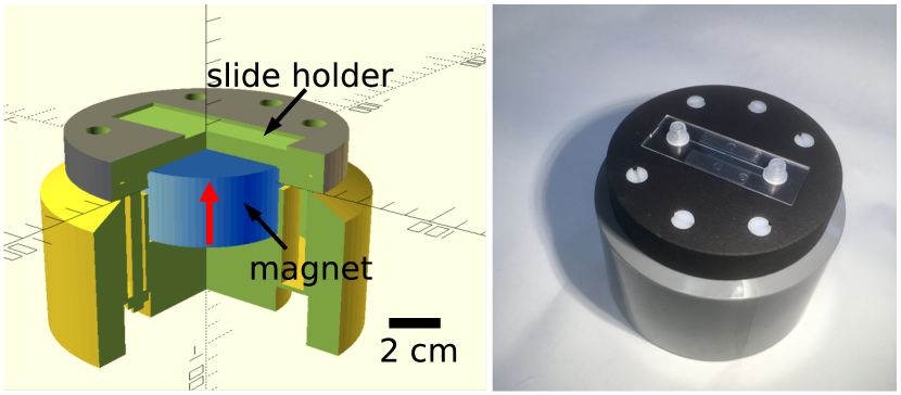
Figure 1: System to investigate the effect of a high magnetic field gradient from a single magnet on the interaction of magnetic nanoparticles on cells. The magnet has a diameter of 70mm and a height of 35mm. The cell culture is located 10.5mm above the magnet in a slide channel.

III.2 Fabrication Halbach magnet system

The Halbach array was assembled from $48$ individual 1.5x1.0x5.0mm magnets (supermagnet.de), see Figure 2. The magnets were placed at a distance on a thin copper foil on a tapered soft magnetic plate and then carefully pushed together. After assembly, the array was glued together using a thin cyanoacrylate glue, and carefully slid off the thin end of the wedge. The array, including the copper foil, was then glued with the foil on top onto a 3D-printed holder. The design for the holder is available in the Supplementary Material.

Figure 2: System to investigate the effect of concentration gradients. A strong field gradient is achieved by means of a Halbach array consisting of $48$ 1.5x1.0x5.0mm magnets (top). The Halbach array (top) is embedded in a 3D-printed holder (center) that keeps the channel slide in place (bottom).

III.3 Magnetic field measurements

The magnetic field above the cylindrical magnet (Figure 3) and Halbach array (Figure 7) was measured with a MetroLab THM1176 three-axis Hall sensor. The sensor was placed at the same height as the channel of the $\mu$-slide and translated using a manual micromanipulator. The location of the probe was estimated to within 1mm and was then fine-tuned laterally to the symmetry in the field profile. The orientation of the probe with respect to the vertical ($z$-axis) is difficult to adjust and could deviate up to $4\mathrm{°}$.

The field profile of the Halbach array was visualized using a magnet viewer, see Figure 7, which has low contrast when the field is parallel to the sheet (TRU components 507706).

III.4 Microscopy

Overview images of the particle distribution in the $\mu$-slide channel were taken by a Canon EOS 800D camera with a Canon EFS18-55 lens at a distance of approximately 20cm, see Figure 8.

The contrast variation over the channel is very low as observed on the cylindrical magnet. For this reason, we mounted the camera in a light-shielded box and illuminated it with a home-built LED ring driven by a constant voltage, see Figure 5. For future experiments, we advise using a constant-current driver to avoid illumination intensity changes during long experiments. Time-lapse images were taken at 2-min intervals using the external shutter input of the Canon camera. The images were then isolated using an optocoupler and driven by an Arduino Uno.

Images were taken using the raw CR2 format (41MB each) until the 64-GB SD card was full (approximately $128$ images). A Python script was used to load the CR2 images and average the pixel intensity $I$ for the green channel over $160$ slices of 16x400pixel (0.2x3.6mm). A reference image was taken from an empty channel ($I_{0}$), and the measured average intensity was converted to absorbance using $\log_{10}(I/I_{0})$.

Higher-resolution images of particle suspension inside the $\mu$-slide channel on top of the cylindrical magnet were taken with a Zeiss Stemi 508 stereo microscope, see Figure 6.

When the $\mu$-slides are removed from their magnet, they can be imaged by transmitted light microscopy. The images in Figure 11 were taken with a Zeiss Axiovert 100 using a 12V 100W halogen light source, a Zeiss LD A-Plan 10$\times$/0.25 Ph1 lens and a Jenoptik Gryphax Prokyon camera. The microscope stage is equipped with stepper motors. To image along the channel, images were taken every 1mm at fixed illumination and combined into a 0.7x36mm image using a Hugin photo stitcher (hugin.sourceforge.io). The intensity profiles were extracted from the stitched images by means of Gwyddion’s “extract profile along arbitrary lines” tool, using the green channel for the bare Fe₂O₃ particles and the red channel for the core-shell particles and a width of 128 pixels.

The $\mu$-slide channels are dedicated to cell studies. Images of cells (Figures 13, 14 and  15) with a size of 2048x2048pixel were taken with a Leica DMi8 fluorescence microscope with a K5 sCMOS camera. Both a $20$$\times$ and a $40$$\times$ lens were used, calibrated at $324$ and 162nm/pixel, respectively. To observe the channels on the Halbach array, we 3D-printed a holder that allowed us to image the location along the channel with a reproducibility of at least $1\text{\,}\mathrm{m}\mathrm{m}$.

III.5 Particles

We used both bare Fe₂O₃ and core-shell magnetic nanoparticle suspensions. The bare Fe₂O₃ suspension was based on iron(III) oxide powder (Alfa Aesar NanoArc, 45007). According to the manufacturer, the particles have a diameter of 2040nm and are over 98 in the $\gamma$ crystal phase. The powder was mixed with demineralized water at an iron concentration of 10.6/. From experiments by Prijic [17] and Rafieepour [13], we esimated that for significant cell mortality, we needed to apply concentrations well above 250/ml. . Therefore, for cell studies on the cylindrical magnet, the stock suspension was diluted $27$ times into a phosphate-buffered saline (PBS) solution with a pH of $7.4$ to achieve an iron concentration of 393(20)/, corresponding to ($2$ to $18$)$\times$e12particles / . For the experiments on the Halbach array, the suspension was diluted further to 100(5)/, so that the expected maximum concentration was approximately equal to the experiment with the cylindrical magnet.

In addition to the bare Fe₂O₃ powder, we used crosslinked dextran iron-oxide cluster-type particles prepared by a core-shell method (Bionized NanoFerrite (BNF) 94-00-102 from Micromod). These particles are red fluorescent (redF) and shipped in a PBS suspension. According to the manufacturer, they have a core of 7580 (w/w) magnetite and a shell of dextran. The particles have a reported diameter of 100nm with a magnetite crystallite diameter of about 20nm. The hydrodynamic diameter of these particles lies between $95$ and 140nm.[36] The original iron concentration as reported by the manufacturer is 6.0/, and particle concentration is 6e12particles/mL. The original suspension was diluted into PBS to achieve an iron concentration of 280(10)/, corresponding to a concentration of 3e12particles / .

Suspensions were kept inside a refrigerator in the dark. Before use, the tubes with suspensions were vigorously shaken and ultrasonically agitated for approximately one minute. For studies that did not involve cells, the PBS was replaced with demineralized water.

III.6 Channel slides

All experiments were performed using Ibidi $\mu$-Slide I Luer channels with an Ibitreat surface coating to promote cell adhesion (Ibidi 80606). The dimension of the channels is 0.8x5.0x50mm.

III.7 Cell staining

Cells were stained for the microscopy images in Figures 13 and 15 with an Iron Stain Kit (ab150674; Abcam, Cambridge, UK). To identify cellular uptake and localization of iron-oxide nanoparticles, HepG2 cells in the $\mu$-slide were washed with PBS and incubated in a mix of potassium ferrocyanide and hydrochloric acid for 3 min. After being rinsed with deionized water, the cells were counterstained with a nuclear fast red solution.

III.8 Mortality assay

For the cell studies (Figures 12 and 14), human hepatoma HepG2 cells (ATCC, HB-8065) were cultured in Eagle’s minimum essential medium supplemented with 10 fetal bovine serum and 1 penicillin-streptomycin in an incubator at 37 and 5 CO₂ atmosphere. The cell concentration was determined by means of a hemocytometer and diluted to 5e4cells/. Of this solution, 200 was introduced into the $\mu$-slide channels. The maximum cell density was 40cells/mm^2.

The Ibidi channels were left inside the incubator for 24hours on top of the holder with and without a magnet before analysis. To assess cell viability, we used a live/dead double-staining assay (Sigma-Aldrich, 04511). Ten fluorescent microscopy images (Leica DMi8) were chosen randomly over the channel area for analysis. Average and standard deviations were calculated from three independent experiments ($30$ images in total).

IV Results and discussion

IV.1 Magnetic field and forces

To verify the calculations of fields and forces, we measured the fields of both the cylindrical magnet and the Halbach array as well as the concentration variation over the channel filled with magnetic nanoparticles.

IV.1.1 Uniform forces: Cylindrical magnet

The force field above the permanent cylindrical magnet varies with distance to the magnet surface in both strength and direction. For experiments with magnetic nanoparticles inside the channel slide, we want the lateral forces in the plane of the channel to be as small as possible, yet the vertical force to be as high as possible and very uniform over the area of interest. Using the soft sphere model of Eq. 3, we determined that the optimal height of the channel slide for both conditions is 10.5mm above the magnet.

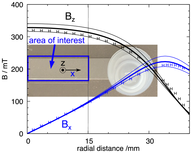
Figure 3: Field strength above the cylindrical magnet showing both calculated and measured vertical (top) and lateral (bottom) field components at the height of the channel slide (10.5mm). Calculated field values for 9.5mm and 11.5mm are shown by thinner lines as well. Assuming a remanent magnetization of 1.30T, the field is predicted within measurement error. Over the length of the channel (30mm), the vector component of the field in the vertical direction is dominant, with a strength greater than 300mT.

Figure 3 shows the measured and calculated magnetic field components perpendicular to channel $B_{\text{z}}$ and along channel $B_{\text{x}}$ at the optimum height of 10.5mm. The measurements follow the prediction quite accurately, but the deviations are greater than the field measurement uncertainty. Additional sources of uncertainty are the angle of the sensor with respect to the magnet’s surface and the distance between the sensor and the magnet’s surface. The latter deviation has a greater impact and may vary over the radial distance. Therefore, we also show predictions that are 1mm higher and lower than the optimum height, respectively. Assuming a remanent magnetization of 1.3T as provided by the manufacturer’s data, the measurements fall in this band within measurement error. Over the length of the channel (30mm, radial distance 15mm), the perpendicular field component is dominant with a value in excess of 300mT. The field strength varies only by 5, and the field angle rotates at a maximum of $\pm$17.

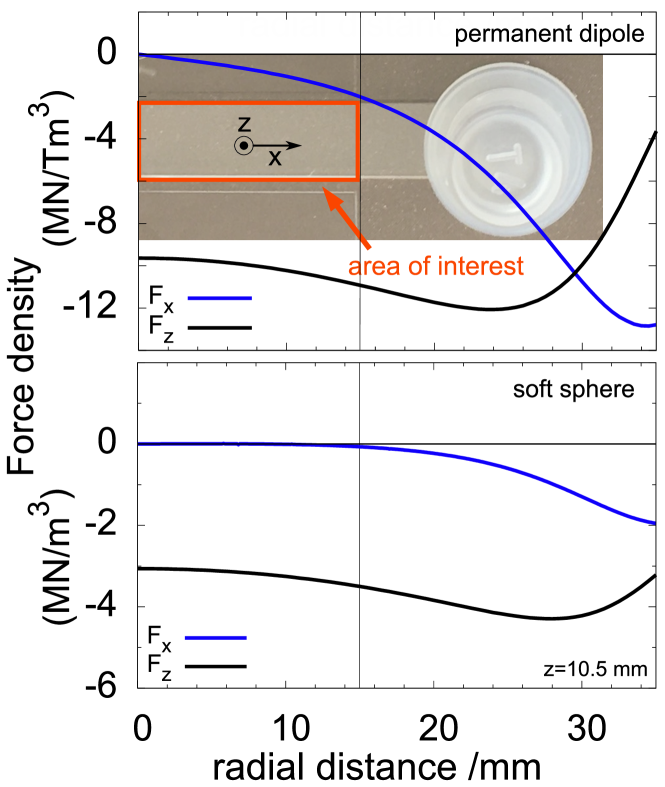
Figure 4: Force densities calculated from the field profiles shown in Figure 3 in vertical (black) and lateral (blue) directions as a function of the position over the length of the channel slide. We apply two extreme models. The top curve shows the result for a model in which we assume that the particle is a permanent magnet with remanent moment $I_{\text{r}}$ (Eq. 2). To obtain the force, multiply by $V_{\text{p}}I_{\text{r}}$. For the bottom curve, we assumed that the particle is a sphere of volume $V_{\text{p}}$ and susceptibility $\chi$ (Eq. 3). To obtain the force, multiply the value on the vertical axis by $3V_{\text{p}}\chi/(3+\chi)$. The vector component of the force in the vertical direction is dominant, with a strength in excess of 3MN/m^3. Over the length of the 30mm channel, the force strength remains within 14 and the force direction varies by less than 1.

Figure 4 shows the calculated forces on particles for both the permanent dipole magnet (top) and soft sphere (bottom) models. For the permanent dipole model, the forces are normalized to the particle magnetic moment $I_{\text{r}}V_{\text{p}}$ [Tm³]. A typical particle has a magnetization in the range from 0.1 to 1T, so force densities are on the order of 1 to 10MN/m^3. For comparison, the gravitation force density on a typical iron-oxide particle is only 40kN/m^3 (standard gravity times mass density difference with water).

For the soft sphere model, the forces are normalized to $3V_{\text{p}}\chi/(3+\chi)$, which ranges from 0 to 3$V_{\text{p}}$. A typical iron-oxide particle has a susceptibility greater than 1 [37], so force densities are in the same range as for the permanent dipole approximation.

Both models show a variation of 14 in the vertical component of the force over the length of the 30-mm channel. The soft sphere model has a much weaker lateral force. At the entrance of the channel, the force tilts only about 1 inward, whereas for the permanent dipole model, it tilts at 10.

Figure 5: Channel filled with core-shell magnetic nanoparticles immediately after filling (top, black) and after 4.3h. The graph shows the absorbance averaged over a 3.6-mm band in the center of the channel, referenced to an empty channel. In the Beer–Lambert approximation, the absorbance is proportional to the concentration. Error bars indicate the standard deviation of the absorbance over the width of the band. The concentration variation over the length of the channel is less than the measurement uncertainty of 12. The reduction in light absorbance with time could also be caused by a gradual decrease in the intensity of the light source. A time-lapse video of the 256-min process is available in the Supplementary Material.

The large magnet produces a very uniform distribution of magnetic particles. Figure 5 shows a channel slide filled with a diluted suspension of 5-nm iron-oxide particles. No concentration gradient can be observed even after more than 4hours. We measured the intensity of the image over a 3.6-mm band over the center of the channel. By comparison with an empty channel, we can measure the concentration variation. Assuming that the logarithm of the ratio of the filled and unfilled channels is proportional to the concentration (Beer–Lambert law), the variation in concentration along the channel is less than the measurement uncertainty of 12. A time-lapse video of the 256-min process with timesteps of 32s is available in the Supplementary Material (CoreShell.mp4). There is a gradual reduction in overall intensity. Closer inspection of the images shows that the magnetic field causes the appearance of many small spots in the case of core-shell particles, see Figure 6, left. We assume that the appearance of these spots is caused by particle clustering, which may explain the reduction in overall reflection of light. Clustering can also be observed for the bare Fe₂O₃ particles, see Figure 6, right.

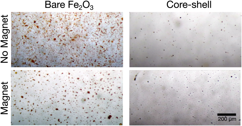
Figure 6: Optical microscopy of bare Fe₂O₃ and core-shell particles without an applied magnetic field (top) and on top of the cylindrical magnet. In the presence of the magnetic field, the particles have a greater tendency to cluster, leading to a reduction of light brown areas in the case of Fe₂O₃ and the appearance of many more small spots in the case of the core-shell particles.

IV.1.2 Concentration gradients: Halbach array

The aim of the large cylindrical magnet described above was to create as uniform a force as possible. If uniformity is not an issue, then a Halbach array can create much higher forces.

Figure 7 (top) shows the calculated and measured magnetic field profiles of a Halbach array of $16$ 1.5x1.0mm magnets. The total width of the array (in $y$-direction) is 15mm. The values of the field components fit very well with measurements if we assume a distance between probe and magnet surface of 0.58mm, which is very reasonable. The maximum field strength is on the order of 400mT, which is comparable to the large cylindrical magnet.

An image of a magnetic viewer film is shown in the background. The light and dark areas indicate regions where the field is parallel and perpendicular to the plane of the viewer film, respectively. The measurement and model show very good qualitative as well as quantitative agreement. There is a small shift in the pattern, which may be caused by the fact that the distance between magnet centers is slightly increased because of the glue used to assemble the array.

Using this model, we can calculate the forces on magnetic nanoparticles. The bottom two graphs in Figure 7 show the in-plane and perpendicular force components for a model, assuming that the nanoparticles are either permanent magnets (center) or soft magnetic spheres (bottom). The perpendicular force is always attractive, and varies by 25 (permanent dipole) to 30 (soft sphere). In contrast, the in-plane force can be both positive and negative. Particles will therefore tend to diffuse to regions where the in-plane force is zero, leading to very non-uniform particle concentrations. However, the force densities are approximately $60$ to $90$ times higher than for the cylindrical magnet. This is the effect of reducing the size of the magnets by a factor of $70$ and using the Halbach configuration.

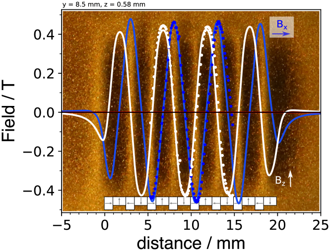
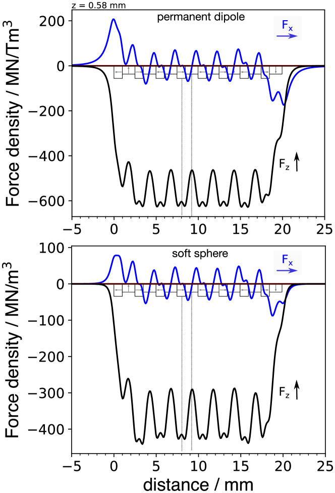
Figure 7: Calculated and measured vertical and lateral components of the field (top) and calculated forces on permanent magnet (center) and soft magnetic sphere (bottom) particles as a function of distance along the Halbach array. To obtain the force, multiply by $V_{\text{p}}I_{\text{r}}$ for the permanent magnet or by $3V_{\text{p}}\chi/(3+\chi)$ for the soft magnetic sphere. In the background of the top field graph, the field direction is shown by means of a magnetic viewer (in the light areas, the field is parallel to the viewer sheet). The circles are measured values. The height was set to 0.58mm in the calculation to match these values. As can be seen by the shift in the measured pattern, the dimensions of the magnets are slightly larger than specified. The field strength is of the same order as was the case for the uniform field in Figure 3. However, the forces are more than one order of magnitude higher because the individual magnets in the Halbach array are $70$ times smaller. In contrast to the cylindrical magnet, the Halbach array has very non-uniform forces, with lateral forces being both positive and negative and vertical forces varying by as much as 30.

In the experiment with the large cylindrical magnet, the channel was filled first with magnetic nanoparticles, so that the concentration distribution was uniform. The channel slide was then carefully lowered vertically along the axis of the magnet to avoid disturbing the concentration. In the case of the Halbach array, we first positioned the empty slide on the array, slightly titled, and filled it from the lower side, see Figure 8. As the suspension flows over the array, particles are trapped by the magnetic field gradient, and the concentration decreases. This achieves a gradient in the concentration. The filling process can be observed in the video in the Supplementary Material (GradientFilling.mov).

As the particles are trapped at the transitions between the magnets, the concentration oscillates slightly. However, the increase in intensity is more or less linear over a range of 12mm (from 820mm). Assuming a Beer–Lambert law for the relation between intensity and concentration, the concentration decreases approximately exponentially. This suggests that a fixed fraction of the particles is indeed captured as the suspension flows over the array.

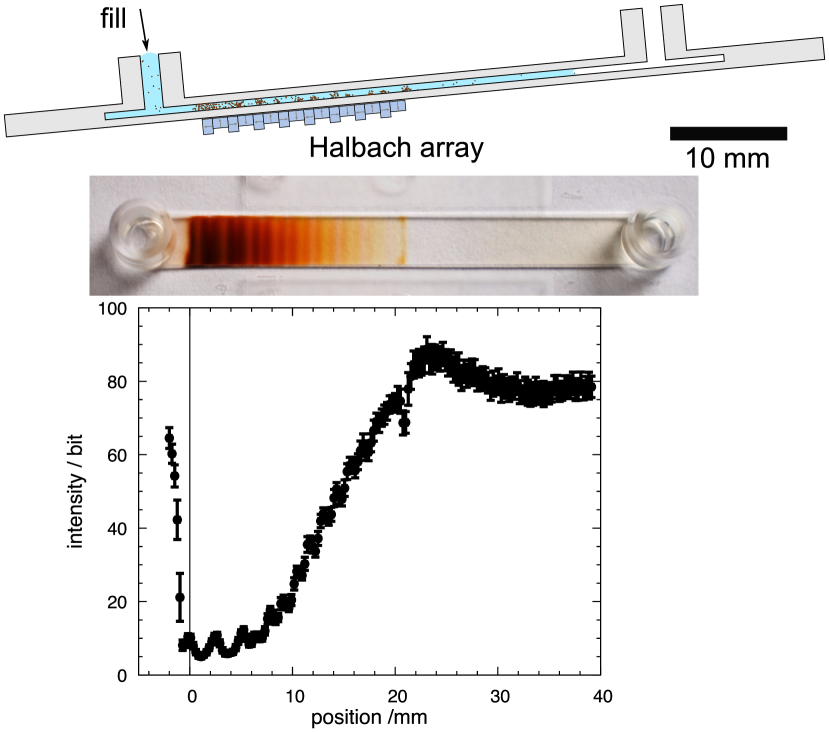
Figure 8: As the channel slowly fills, bare Fe₂O₃ nanoparticles are captured in the stray field of the Halbach array. Particles are captured as the fluid moves over the array, leading to a concentration gradient. The contrast of the image is shown below and increases almost linearly from 5 to 90bit in the range of 820mm. On the basis of the Beer–Lambert law, we conclude that there is a logarithmic reduction in concentration in this region. A video of the filling process (GradientFilling.mov) is available in the Supplementary Material.

The velocity of the particles with respect to the fluid is determined by the balance between magnetic and drag force. Using the magnetic force calculated by the permanent dipole model and assuming a parabolic flow profile, we can calculate the trajectories of magnetic nanoparticles in suspension, see Section II.2. Figure 9 shows an example of magnetic nanoparticles with a radius of 67nm and a remanent magnetization of 1.0T in a flow with an average velocity of 25mm/s. For this particular situation, about half the particles are trapped on the array, whereas the other half leaves the channel slide. Particles at the bottom of the channel are captured more easily. Using this type of calculation, we can predict a capture height and capture efficiency. In this particular calculation, the capture height is 0.4mm and the capture efficiency is 50.

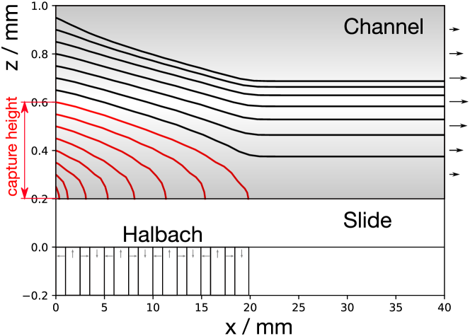
Figure 9: Calculated trajectories of magnetic nanoparticles released at the left-hand side of the Halbach array. The flow profile in the channel is assumed to be of parabolic shape with an average flow velocity of 25mm/s, or 6mL/min. Note that the $x$ and $z$ scales of the image are very different. The particular example we have chosen here illustrates the situation where 50 are captured (particles with a radius of 67nm and magnetic remanence of 1.0T.)

The magnetic force of the particles in the suspension scales with their volume, whereas the drag force scales with the radius. The smaller the particles, the less chance they have of being captured. Figure 10 shows the estimated capture height and capture efficiency as a function of particle radius (again assuming particles with a remanent magnetization of $1.0\text{\,}\mathrm{T}$). Up to a particle radius of about 75nm, the capture rate increases linearly with particle radius. Owing to the parabolic flow profile, the capture efficiency increases quadratically. Particles with radii above 110nm are all captured. Particles with radii of less than 20nm have a chance of less than 7 of being captured in this specific situation.

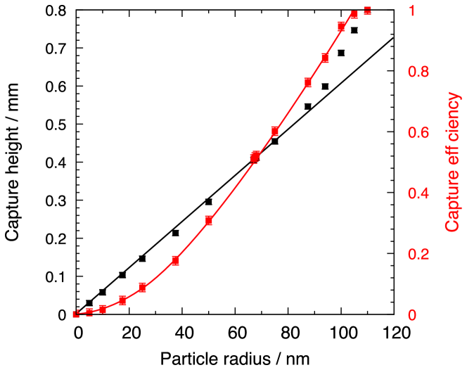
Figure 10: Calculated capture height, see Figure 9 (left axis, black) and resulting capture efficiency (right axis, red) as a function of particle radius. The capture rate for particles with radii below 20nm is less than 7. Owing to the parabolic flow profile, the capture efficiency increases quadratically with increasing particle radius. A capture efficiency of 50 is reached for a particle radius of about 67nm, which is the example shown in Figure 9. For small particle radii, the capture height increases linearly with increasing particle radius. Above this value, the linear relationship between capture height and radius is lost. The red line is not a fit, but shown merely to guide the eye. Full capture is achieved for particle radii above 110nm.

Experiments on liver cell viability were performed with bare Fe₂O₃ particles, as described above, as well as with core-shell magnetic nanoparticles. Figure 11 shows stitched microscope images over the length of the channel slide for both types of particles. The gradient in particle concentration is clearly visible. The black dots at the entry of the channel with the Fe₂O₃ suspension are gas bubbles. These bubbles did not form in the suspension of core-shell particles. The Fe₂O₃ particles show a less uniform distribution. Rather, the particles cluster into elongated structures with lengths up to 100. At the start of the Halbach array, these clusters are irregularly distributed. Further into the channel, the distribution becomes more regular. Above the in-plane magnets of the array, the clusters align along the channel; above the perpendicular magnets, the clusters are oriented more randomly. Not all particles are captured by the Halbach array. At the end of the array, a number of larger clusters can be found. In the remaining part of the channel, chains of particles can be seen aligned very well along the channel length. For the Fe₂O₃ particles, this alignment is lost towards the end of the channel. In the case of the core-shell particles, the alignment turns towards 45 at the end of the channel.

In the case of bare Fe₂O₃ particles, we observed the formation of tiny bubbles at the entry of the channel. We have two hypotheses regarding the origin of these bubbles. They could be caused by heating of the fluid due to the intense illumination in the microscope. The increased temperature of the fluid could trigger the release of dissolved gases (nitrogen, oxygen). Indeed, we have been able to melt the channel slide by using full-intensity light, so an increase in temperature is very likely. However, the channel filled with core-shell particles did not show bubble formation, not even in the very dark, i.e. light-absorbing, area from 03mm. Bubbles formed also at moderate light intensity, see Supplementary Materials, video Fe2O3.mp4. Our other hypothesis is that Fe₂O₃ causes photo-oxidation of water, releasing hydrogen and oxygen.[38] Indeed, when a suspension of bare Fe₂O₃ is placed in sunlight, gas bubbles are produced continuously for days. In the case of core-shell particles, the dextran shell may prevent contact between water and the Fe₂O₃, which could explain the absence of bubbles. Further research will be required to determine the origin of the bubbles. In any case, if the concentrations are low and/or illumination is moderate, bubbles do not form.

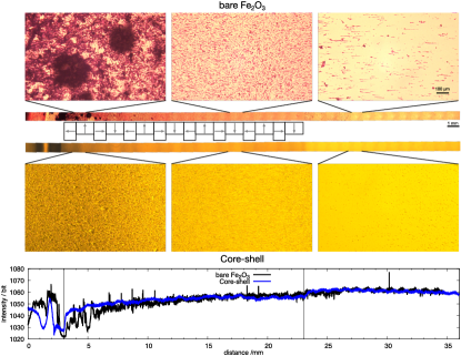
Figure 11: Microscopy images of bare Fe₂O₃ (top) and core-shell particles (bottom) after the channel slide is removed from the Halbach array. The images were stitched to visualize a $36$$\times$0.7mm^2 band along the center of the channel and are available in full resolution in the Supplementary Material (FullGradient*.png). Typical examples are extracted, and the estimated location of the Halbach array is shown. The bare Fe₂O₃ particles show a more non-uniform distribution. Particles tend to cluster into structures that can be as long as 100. At the start of the Halbach array, the clusters are irregularly distributed. Midway through the array, the clusters align along the channel. Not all particles are captured. Those that escape the Halbach array tend to align into chains along the channel length. The bottom graph shows intensity profiles along the stitched images for both types of particles. The change in intensity along the channel is stronger for the bare Fe₂O₃ particles. The strong variation at the start of the array is caused by the gas bubbles.

IV.2 Cell viability

We demonstrated the use of two designs on human hepatoma HepG2 cells in channel slides. The viability of the cells in the presence of magnetic nanoparticles was observed over a period of one to six days.

IV.2.1 Cylindrical Magnet

Figure 12 shows the viability of HepG2 cells inside channel slides after six days, with and without application of a uniform magnetic force and with and without the presence of magnetic nanoparticles. The application of a magnetic force by itself does not significantly affect cell viability. However, when there are magnetic nanoparticles in the solution, the application of a magnetic force strongly reduces cell viability. The effect is similar for bare Fe₂O₃ and core-shell nanoparticles. There seems to be a small reduction in cell death when magnetic nanoparticles are added. However, this effect is only statistically significant for the core shell particles.

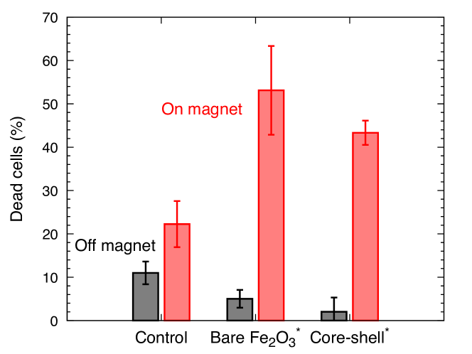
Figure 12: Human hepatoma HepG2 cell mortality after $6\text{\,}\mathrm{d}\mathrm{a}\mathrm{y}\mathrm{s}$, with (red) and without (black) application of a uniform magnetic field. Error bars indicate the standard error, based on ten images per slide and three independent experiments. The control without magnetic particles shows that the magnetic field by itself has no statistically significant effect on cell mortality (confidence less than $95\text{\,}\mathrm{\char 37\relax}$). The presence of bare Fe₂O₃ particles at a concentration of $400\text{\,}\mathrm{\SIUnitSymbolMicro}\mathrm{g}\mathrm{/}\mathrm{m}\mathrm{L}$ and core-shell particles at $280\text{\,}\mathrm{\SIUnitSymbolMicro}\mathrm{g}\mathrm{/}\mathrm{m}\mathrm{L}$ increases cell mortality up to approximately $50\text{\,}\mathrm{\char 37\relax}$ (confidence exceeds $99\text{\,}\mathrm{\char 37\relax}$).

Closer inspection of the cells and nanoparticles in the channel slides shows that, on the magnet, the nanoparticles tend to cluster more strongly, see Figure 13. The effect is strongest for the bare Fe₂O₃ particles, which form elongated structures with lengths of up to 100. However, cell morphology does not seem to be strongly affected by the application of a magnetic force.

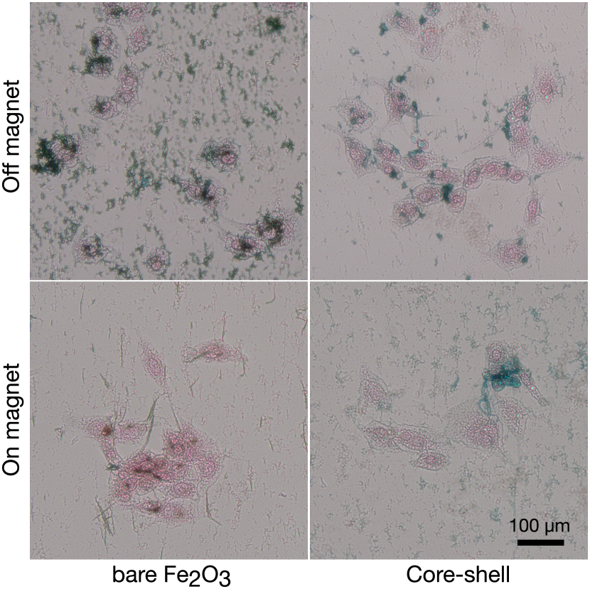
Figure 13: Optical microscopy image of HepG2 cells cultivated for six days in the presence of bare Fe₂O₃ (left, $400\text{\,}\mathrm{\SIUnitSymbolMicro}\mathrm{g}\mathrm{/}\mathrm{m}\mathrm{L}$) and core-shell particles (right, $280\text{\,}\mathrm{\SIUnitSymbolMicro}\mathrm{g}\mathrm{/}\mathrm{m}\mathrm{L}$). The top and bottom rows show cells that were cultivated off- and on-magnet, respectively. The nuclei in the cells are stained red; the iron-oxide is stained blue. Cell morphology is not noticeably dependent on the type of particles. In the magnetic field, the particles agglomerate into chains. This effect is strongest for the bare Fe₂O₃ nanoparticles.

IV.2.2 Halbach array

Figure 14, top, shows the viability of HepG2 cells in the presence of bare Fe₂O₃ nanoparticles with an average concentration of 100g/mL. If the channel slide is not positioned on the Halbach array (“control”), the nanoparticles have no effect on cell viability. This is in agreement with experimental results for the cylindrical magnet.

If the channel with HepG2 cells is filled when it is positioned on top of the Halbach array, a gradient forms. If it is kept there for several days, cell viability strongly decreases. The decrease is strongest at the start of the channel where the concentration is highest. From 15mm onwards, there is no difference in the control.

If we assume that all particles are captured on the array, i.e. on the first half of the microslide, the average concentration doubles to 200g / mL. Taking the intensities extracted from Figure 11, we can use the Beer–Lambert model to estimate the concentration as a function of position. With a single experiment, we can therefore obtain a first estimate of cell viability versus concentration. The result is shown in Figure 14 (bottom). Cells in areas where the concentration is below 75g/mL are not noticeably affected.

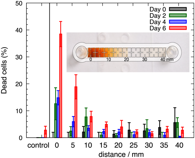
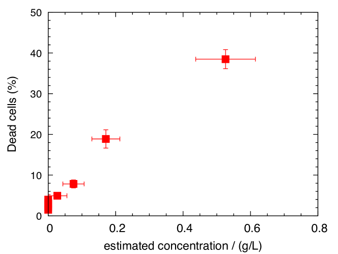
Figure 14: Top: Viability of HepG2 cells cultivated in the presence of bare Fe₂O₃ nanoparticles with concentration decreasing to zero at about $20\text{\,}\mathrm{m}\mathrm{m}$ as a function of time. Error bars indicate the standard error, based on ten images per slide and three independent experiments. As the control (left), a channel slide without magnetic particles was analyzed at day 6. Bottom: Viability at day 6 as a function of nanoparticle concentration, estimated based on intensity gradients as shown in Figure 11 and the Beer–Lambert law. Error bars indicate the standard error for the fraction of dead cells and standard deviation for the estimated concentration. Cell mortality increases with increasing concentration and time up to $40(5)\text{\,}\mathrm{\char 37\relax}$ at the highest concentration after 6 days of exposure. Cells at a distance of $15\text{\,}\mathrm{m}\mathrm{m}$ and above, i.e. with concentrations below $75\text{\,}\mathrm{\SIUnitSymbolMicro}\mathrm{g}\mathrm{/}\mathrm{m}\mathrm{L}$, are not noticeably affected.

V Conclusions

We constructed magnetic systems that exert a strong force on magnetic nanoparticles inside a channel slide with a two-dimensional human liver cell culture. These systems were used to assess the effect of these magnetic forces on the mortality of mixtures of liver cells and nanoparticles. The nanoparticles we used were bare Fe₂O₃ with diameters of $20$ to 40nm and core-shell particles of 100nm diameter with a magnetite core and a cross-linked dextran shell.

The first system we investigated exerts a uniform force over the entire channel via a cylindrical magnet with a diameter of 70mm. The vector components of the field and force in the vertical direction are dominant, with a strength in excess of 300mT and 6MN/m^3, respectively. Over the length of the 30-mm channel, the force strength remains within 14, and the force direction varies by less than 1, leading to a concentration gradient that is less than the measurement uncertainty of 12 after 4.3h exposure. Application of a magnetic field leads to an increased clustering of particles, both for bare Fe₂O₃ and core-shell nanoparticles.

The second system is based on a Halbach array that applies non-uniform fields, the strength of which is on the same order as the field of the large magnet of the first system. However, the forces are more than one order of magnitude higher because the individual magnets in the Halbach array are $70$ times smaller. Owing to the Halbach configuration, the lateral forces are both positive and negative and attract particles toward the transitions. The vertical forces are always downward but vary up to 30.

When a suspension of bare Fe₂O₃ is passed over the Halbach array, particles are captured, and the concentration in the flow diminishes as the wavefront progresses. As a result, a gradient in particle concentration is achieved over the length of the Halbach array.

Calculations show that particles with a radius of less than 20nm and a remanent magnetization of 1T are trapped above the Halbach array with an efficiency of less than 7. However, our results show that we are able to capture most of the Fe₂O₃ particles. Therefore, we conclude that clustering already takes place in suspension. Calculations show that clusters with a diameter of 67nm and a remanence of 1T are captured with an efficiency of 51. For cluster radii below this value, capture height increases linearly with increasing radius. Above this value, capture efficiency increases rapidly, and full capture is achieved for cluster radii greater than 110nm.

We observed that particles form clusters of structures with lengths of up to 100 at the bottom of the channel. At the start of the Halbach array, these clusters are distributed irregularly. Midway through the array, however, the distribution becomes more regular. Above the in-plane magnets of the array, the clusters align along the channel, whereas above the perpendicular magnets, the clusters become oriented more randomly. Not all particles are captured by the Halbach array. At the end of the array, a number of larger clusters can be found. In the remainder of the channel, chains of particles can be seen aligned along the channel length.

Both systems demonstrate cell survival in the presence of magnetic nanoparticles and strong magnetic field gradients. Application of a uniform magnetic force reduces the viability of liver cells in the presence of bare Fe₂O₃ as well as core-shell nanoparticles by approximately 50. Cell morphology is not noticeably dependent on the type of particles, but the presence of the magnetic field has a strong influence on their distribution. In the magnetic field, the particles agglomerate into chains. This effect is strongest for the bare Fe₂O₃ nanoparticles.

The Halbach array allows us to analyze the cell response as a function of concentration. In a gradient of Fe₂O₃ nanoparticles, cell mortality depends on the local concentration, ranging from 40(5) after six days of exposure at the highest concentration of approximately 500g/mL to indistinguishable from the control at a concentration of less than 75g/mL.

The models presented in this paper offer a solid basis for designing magnetic systems for cell culture studies and particle trapping. These design methodologies, together with the tools available online, can be used to modify designs for other channel geometries. The simulation tools presented here for analyzing particle trajectories can serve as a fast alternative to finite-element simulations.[30] The capability of creating concentration gradients may speed up the screening of the effect of magnetic particles on cell lines. It may also allow other applications, such as cell migration studies.[39]

Appendix A Supplementary Material

A.1 Optical microscope of stained cells and bare Fe₂O₃ nanoparticles

Figure 15 shows optical microscopy images of bare Fe₂O₃ nanoparticles in combination with cells (similar to Figure 13) as a function of the position in the channel. From left to right, the particle concentration decreases, as indicated by the positions on the image of the slide channel below. (For clarity, note that this is the image of Figure 8 that was at higher concentration and without cells. The actual particle density is more comparable to Figure 11.) The cell morphology does not vary significantly with nanoparticle concentration. The increase in nanoparticle concentration is clearly visible, but the concentration is non-uniform over length scales comparable to the cell dimensions.

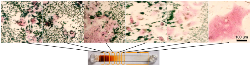
Figure 15: Optical microscopy of cells (stained red) and bare Fe₂O₃ nanoparticles (stained blue) inside the channel slides after 4 days of cultivation.

A.2 Cades input files

The compressed folder Cades.zip contains the source files for the MagMMEMS package. They are used to calculate the magnetic field and forces of the cylindrical magnet, see Section II.1.

A.3 Python source files

The Python source code used to calculate the trajectories of particles above the Halbach array is available on github: https://github.com/LeonAbelmann/Trajectory

A.4 3D-print source files

The OpenScad source files (*.scad) and print files (*.stl) for the 3D-printed holders are available in the compressed folder 3Dprints.zip.

A.5 Time-lapse videos

The time-lapse video CoreShell.mp4 shows the change in concentration over time, see Figure 5. Also shown is the same experiment for the bare Fe₂O₃ suspension, Fe2O3.mp4, where the formation of gas bubbles can be observed.

A.6 Gradient filling

The formation of the concentration gradient can be observed in the video GradientFilling.mp4. The end result is shown in Figure 8.

A.7 High resolution stiched images

Figures FullGradientFe2O3.png and FullGradientCoreShell.png show high-resolution versions of the images in Figure 11.

References

- Elsaesser and Howard [2012] A. Elsaesser and C. V. Howard, Advanced Drug Delivery Reviews 64, 129 (2012).
- Anselmo and Mitragotri [2016] A. C. Anselmo and S. Mitragotri, Bioengineering & translational medicine 1, 10 (2016).
- Mornet et al. [2004] S. Mornet, S. Vasseur, F. Grasset, and E. Duguet, Journal of Materials Chemistry 14, 2161 (2004).
- Pankhurst et al. [2003] Q. A. Pankhurst, J. Connolly, S. K. Jones, and J. Dobson, Journal of physics D: Applied physics 36, R167 (2003).
- Zabow et al. [2011] G. Zabow, S. Dodd, E. Shapiro, J. Moreland, and A. Koretsky, Magnetic Resonance in Medicine 65, 645 (2011).
- Teeguarden et al. [2006] J. G. Teeguarden, P. M. Hinderliter, G. Orr, B. D. Thrall, and J. G. Pounds, Toxicological Sciences 95, 300 (2006).
- Vazquez-Muñoz et al. [2017] R. Vazquez-Muñoz, B. Borrego, K. Juárez-Moreno, M. García-García, J. D. M. Morales, N. Bogdanchikova, and A. Huerta-Saquero, Toxicology Letters 276, 11 (2017).
- Greulich et al. [2012] C. Greulich, D. Braun, A. Peetsch, J. Diendorf, B. Siebers, M. Epple, and M. Köller, RSC Advances 2, 6981 (2012).
- Pondman et al. [2014] K. Pondman, N. Bunt, A. Maijenburg, R. van Wezel, U. Kishore, L. Abelmann, J. ten Elshof, and B. Ten Haken, Journal of Magnetism and Magnetic Materials 380, 299 (2014).
- Kim et al. [2010] D. . H. Kim, E. A. Rozhkova, I. V. Ulasov, S. D. Bader, T. Rajh, M. S. Lesniak, and V. Novosad, Nature Materials 9, 165 (2010).
- Kilinc et al. [2016] D. Kilinc, C. Dennis, and G. Lee, Advanced Materials , 5672 (2016).
- Colombo et al. [2012] M. Colombo, S. Carregal-Romero, F. Casula M., L. Gutiérrez, P. Morales M., B. Bahm I., J. T. Heverhagen, D. Prosperi, and W. J. Parak, Chemical Society Reviews 41, 4306 (2012).
- Rafieepour et al. [2019] A. Rafieepour, M. R. Azari, H. Peirovi, F. Khodagholi, J. P. Jaktaji, Y. Mehrabi, P. Naserzadeh, and Y. Mohammadian, Toxicology and Industrial Health 35, 703 (2019).
- Berry et al. [2003] C. C. Berry, S. Wells, S. Charles, and A. S. Curtis, Biomaterials 24, 4551 (2003).
- Soenen and Cuyper [2010] S. J. Soenen and M. D. Cuyper, Nanomedicine 5, 1261 (2010).
- Yanai et al. [2012] A. Yanai, U. O. Häfeli, A. L. Metcalfe, P. Soema, L. Addo, C. Y. Gregory-Evans, K. Po, X. Shan, O. L. Moritz, and K. Gregory-Evans, Cell Transplantation 21, 1137 (2012).
- Prijic et al. [2010] S. Prijic, J. Scancar, R. Romih, M. Cemazar, V. B. Bregar, A. Znidarsic, and G. Sersa, The Journal of Membrane Biology 236, 167 (2010).
- Haim et al. [2004] H. Haim, I. Steiner, and A. Panet, Journal of Virology 79, 622 (2004).
- Scherer et al. [2002] F. Scherer, M. Anton, U. Schillinger, J. Henke, C. Bergemann, A. Krüger, B. Gänsbacher, and C. Plank, Gene therapy 9, 102 (2002).
- Pickard and Chari [2010] M. Pickard and D. Chari, Nanomedicine 5, 217 (2010).
- Dejardin et al. [2011] T. Dejardin, J. de la Fuente, P. del Pino, E. P. Furlani, M. Mullin, C.-A. Smith, and C. C. Berry, Nanomedicine 6, 1719 (2011).
- Venugopal et al. [2016] I. Venugopal, S. Pernal, A. Duproz, J. Bentley, H. Engelhard, and A. Linninger, Materials Research Express 3, 095010 (2016).
- Park et al. [2016] J. Park, N. R. Kadasala, S. A. Abouelmagd, M. A. Castanares, D. S. Collins, A. Wei, and Y. Yeo, Biomaterials 101, 285 (2016).
- Joshi et al. [2015] P. Joshi, P. S. Williams, L. R. Moore, T. Caralla, C. Boehm, G. Muschler, and M. Zborowski, Analytical Chemistry 87, 9908 (2015).
- Riegler et al. [2011] J. Riegler, K. D. Lau, A. Garcia-Prieto, A. N. Price, T. Richards, Q. A. Pankhurst, and M. F. Lythgoe, Medical Physics 38, 3932 (2011).
- Shen et al. [2017] W.-B. Shen, P. Anastasiadis, B. Nguyen, D. Yarnell, P. J. Yarowsky, V. Frenkel, and P. S. Fishman, Cell Transplantation 26, 1235 (2017).
- Hoffmann et al. [2002] C. Hoffmann, M. Franzreb, and W. Holl, IEEE Transactions on Appiled Superconductivity 12, 963 (2002).
- Gomes et al. [2018] C. S. Gomes, A. Fashina, A. Fernández-Castané, T. W. Overton, T. J. Hobley, E. Theodosiou, and O. R. Thomas, Journal of Chemical Technology & Biotechnology 93, 1901 (2018).
- Kang et al. [2012] J. H. Kang, S. Krause, H. Tobin, A. Mammoto, M. Kanapathipillai, and D. E. Ingber, Lab on a Chip 12, 2175 (2012).
- Stevens et al. [2021] M. Stevens, P. Liu, T. Niessink, A. Mentink, L. Abelmann, and L. Terstappen, Diagnostics 11, 1020 (2021).
- Xue et al. [2019] M. Xue, A. Xiang, Y. Guo, L. Wang, R. Wang, W. Wang, G. Ji, and Z. Lu, RSC Advances 9, 38496 (2019).
- Ooi et al. [2013] C. Ooi, C. M. Earhart, R. J. Wilson, and S. X. Wang, IEEE Transactions on Magnetics 49, 316 (2013).
- Alon et al. [2015] N. Alon, T. Havdala, H. Skaat, K. Baranes, M. Marcus, I. Levy, S. Margel, A. Sharoni, and O. Shefi, Lab on a Chip 15, 2030 (2015).
- Delinchant et al. [2007] B. Delinchant, D. Duret, L. Estrabaut, L. Gerbaud, H. Nguyen Huu, B. Du Peloux, H. L. Rakotoarison, F. Verdière, and F. Wurtz, COMPEL-The international journal for computation and mathematics in electrical and electronic engineering 26, 368 (2007).
- Midelet et al. [2017] J. Midelet, A. H. El-Sagheer, T. Brown, A. G. Kanaras, and M. H. V. Werts, Particle & Particle Systems Characterization 34, 1700095 (2017).
- Giustini et al. [2009] A. J. Giustini, R. Ivkov, and P. J. Hoopes, in Energy-based Treatment of Tissue and Assessment V, edited by T. P. Ryan (SPIE, 2009).
- Yun et al. [2014] H. Yun, X. Liu, T. Paik, D. Palanisamy, J. Kim, W. D. Vogel, A. J. Viescas, J. Chen, G. C. Papaefthymiou, J. M. Kikkawa, M. G. Allen, and C. B. Murray, ACS Nano 8, 12323 (2014).
- Kay et al. [2006] A. Kay, I. Cesar, and M. Grätzel, Journal of the American Chemical Society 128, 15714 (2006).
- Greiner et al. [2014] A. M. Greiner, M. Jäckel, A. C. Scheiwe, D. R. Stamow, T. J. Autenrieth, J. Lahann, C. M. Franz, and M. Bastmeyer, Biomaterials 35, 611 (2014).