Anisotropy in the dielectric function of Bi₂Te₃ from first principles: From the UV-visible to the infrared range

Abstract

The dielectric properties of Bi₂Te₃, a layered compound crystallizing in a rhombohedral structure, are investigated by means of first-principles calculations at the random phase approximation level. A special attention is devoted to the anisotropy in the dielectric function and to the local field effects that strongly renormalize the optical properties in the UV-visible range when the electric field is polarized along the stacking axis. Furthermore, both the Born effective charges for each atom and the zone center phonon frequencies and eigenvectors needed to describe the dielectric response in the infrared range are computed. Our theoretical near-normal incidence reflectivity spectras in both the UV-visible and infrared range are in fairly good agreement with the experimental spectras, provided that the free carriers Drude contribution arising from defects is included in the infrared response. The anisotropic plasmon frequencies entering the Drude model are computed within the rigid band approximation, suggesting that a measurement of the reflectivity in the infrared range for both polarizations might allow to infer not only the type of doping but also the level of doping.

I INTRODUCTION

A great deal of interest has been focused on Bi₂Te₃ because of its outstanding thermoelectric properties at room temperature arising from both a narrow gap electronic structure and a low thermal conductivitysnyder_2008 . The more recent discovery of three-dimensional topological insulators has renewed the interest for this compound. Indeed, soon after Bi₂Te₃ was theoretically predicted to host topologically non trivial metallic surface states with a Dirac-like dispersion around the surface Brillouin zone centerzhang_2009 , some angular-resolved photoemission spectroscopy (ARPES) studies revealed the existence of such linearly dispersing surface stateschen_2009 ; hsieh1_2009 ; hsieh2_2009 . While these extraordinary electronic properties encoded in the bulk wavefunctions have been thoroughly investigated both experimentallykohler1_1976 ; kohler2_1976 ; mohelsky_2020 ; hajlaoui_2012 ; weis_2021 and theoreticallywang_2007 ; luo_2012 ; kioupakis_2010 ; yazyev_2012 ; aguilera_2013 ; nechaev_2013 , the infrared (IR) and optical responses have been studied more sparselyrichter_1977 ; chapler_2014 ; Greenaway_1965 ; dubroka_2017 , notwithstanding the fact that applications in the technology relevant IR to visible range have been envisionned. Indeed, experiments have shown that Bi₂Te₃ can support surface plasmons in the entire visible rangezhao_2015 and some ellipsometry measurements even suggest that Bi₂Te₃ is a natural hyperbolic material in the near-IR to visible spectral range with appealing applications like hyperresolved superlensingesslinger_2014 . Surprisingly, the optical properties infered from reflectivity spectrasGreenaway_1965 or ellipsometry measurementsdubroka_2017 ; zhao_2015 ; esslinger_2014 are rather scattered. Hence, it’s important to compute reference optical properties at a given level of theoryonida_2002 that can be directly compared to the available experimental results. Such a confrontation between theory and experiment is crucial not only to refine the level of theory needed to achieve a good description of the experimental results but also to spur new experiments guided by theory.

The paper is organized as follows. In section II, we give an account of the technicalities used to perform our first-principles calculations. In section III, we describe the crystallographic structure of Bi₂Te₃ and compare our calculated lattice constants and internal coordinates to the experimental values extracted from X-ray measurements. In section IV, we discuss the rather complex bandstructure including spin-orbit coupling (SOC) computed within the local density approximation (LDA) and show that the band gaps, as expected and already demonstrated in other theoretical studieskioupakis_2010 ; yazyev_2012 ; aguilera_2013 ; nechaev_2013 , are underestimated with respect to the values infered from optical spectroscopy measurements. In section V, we compute the optical properties within the random phase approximation (RPA) for an electric field either parallel or perpendicular to the stacking axis, discuss the crucial role of local field (LF) effects and make a direct comparison with available experimental results. In section VI, we compare our calculated zone center phonon frequencies to the frequencies extracted from both Raman and infrared (IR) spectroscopy measurements. In section VII, we compute the Born effective charge tensors that are key ingredients to compute the IR dielectric tensor. In section VIII, we derive the formalism used to compute the IR dielectric tensor with our home made code and discuss the anisotropy in our computed dielectric tensor for frequencies in the THz range. In section IX, we compute the normal incidence reflectivity spectras for both polarizations and only partially reproduce the experimental spectras because free carriers arising from defects contribute to the IR dielectric tensor and lead to a drastic change in the calculated spectras. Finally, in section X, we compute the anisotropic plasmon frequencies using a rigid band approximation for different type and level of doping. A direct comparison with the fitted plasmon frequencies used in part IX to reproduce the experimental spectras seems to indicate that it might be possible to infer not only the type of doping but also the level of doping from our calculations.

II COMPUTATIONAL DETAILS

All the calculations are done within the framework of the local density approximation (LDA) for the exchange-correlation functional to density functional theory (DFT) using the ABINIT codegonze_2009 ; gonze_2016 . Relativistic separable dual-space Gaussian pseudo-potentialshartwigsen_1998 are used with Bi ($6s^{2}6p^{3}$) and Te ($5s^{2}5p^{4}$) levels treated as valence states. Spin-orbit coupling is included and an energy cut-off of 40 Hartree in the planewave expansion of wavefunctions together with a $16\times 16\times 16$ kpoint grid for the Brillouin zone integration are used.

III LATTICE PARAMETERS AND INTERNAL COORDINATES

Table 1: Calculated LDA lattice parameters and internal parameters including spin-orbit coupling (SOC) compared to both existing experimentalfrancombe_1958 ; wiese_1960 and theoreticalluo_2012 results.

	Rhombohedral structure			Hexagonal structure		Internal parameters
	$a_{0}$ (Å)	$\alpha_{0}$ (o)	$V_{0}$ (Å3)	$a_{\parallel,0}$ (Å)	$a_{\perp,0}$ (Å)	$\nu$ (Te)	$\mu$ (Bi)
Expt.francombe_1958 ; wiese_1960	10.473	24.159	169.10	30.487	4.383	0.2095	0.4001
This work (0 K)	10.214	24.706	163.71	29.692	4.370	0.2071	0.4009
LDA+SOCluo_2012	10.124	24.806	160.65	29.423	4.349	0.2063	0.4012
This work (300 K)	10.473	24.159	169.10	30.487	4.383	0.2091	0.4002

Bi₂Te₃ crystallizes in a rhombohedral structure, also called A7 structure, with five atoms per unit cell. The vectors spanning the unit cell are given by

$${\bf{a}}_{1}=\left(a\xi,-\frac{a\xi}{\sqrt{3}},h\right);{\bf{a}}_{2}=\left(0,\frac{2a\xi}{\sqrt{3}},h\right);{\bf{a}}_{3}=\left(-a\xi,-\frac{a\xi}{\sqrt{3}},h\right),$$ (1)

where $\xi=\sin[\frac{\alpha}{2}]$ and $h=a\sqrt{1-\frac{4}{3}\xi^{2}}$. The length of the three lattice vectors is equal to $a$ and the angle between any pair of vector is $\alpha$. The three Te atoms can be classified into two inequivalent types. Two of them, labelled as Te₁, are located at $\pm\nu{\bf{c}}$ while the last Te atom, labelled as Te₂, is set at the origin. The two Bi atoms are equivalent and located at $\pm\mu{\bf{c}}$. Here $\nu$ and $\mu$ are dimensionless parameters and ${\bf{c}}={\bf{a}}_{1}+{\bf{a}}_{2}+{\bf{a}}_{3}$ is parallel to the trigonal axis (C₃ axis). The rhombohedral structure is depicted in Fig. 1(a).

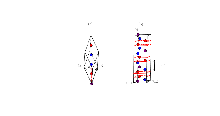
Figure 1: (a) Rhombohedral structure with 5 atoms per unit cell. The two Te₁ atoms, the Te₂ atom and the two Bi atoms are respectively colored in red, purple and blue. (b) Hexagonal structure with 15 atoms per unit cell. The planes containing Te₁ atoms are highligthed and one quintuple layer (QL) Te₁-Bi-Te₂-Bi-Te₁ is shown.

Alternatively, the structure can be viewed as an hexagonal structure depicted in Fig. 1(b) and spanned by the following three lattice vectors

$${\bf{a}}_{\perp,1}={\bf{a}}_{1}-{\bf{a}}_{2};~{}{\bf{a}}_{\perp,2}={\bf{a}}_{2}-{\bf{a}}_{3};~{}{\bf{a}}_{\parallel}={\bf{c}},$$ (2)

where $a_{\perp,1}=a_{\perp,2}\equiv a_{\perp}$. The lattice cell parameters of the two structures are related to each other by the following relations

$$\begin{array}[]{lcl}a_{\perp}=2a\sin\left(\frac{\alpha}{2}\right)&&a=\frac{1}{3}\sqrt{3a_{\perp}^{2}+a_{\parallel}^{2}}\\ a_{\parallel}=a\sqrt{3+6\cos(\alpha)}&&\sin\left[\frac{\alpha}{2}\right]=\frac{3}{2}a_{\perp}/\sqrt{3a_{\perp}^{2}+a_{\parallel}^{2}.}\end{array}$$ (3)

The hexagonal structure is easier to visualize as compared to the rhombohedral structure and can be viewed as made of three quintuple layers Te₁-Bi-Te₂-Bi-Te₁. However, it’s worth noting that all the calculations have been performed using the rhombohedral structure because it contains three times atoms less than the hexagonal structure.

The calculated LDA lattice parameters including spin-orbit coupling (SOC) are displayed in table 1 and compared to the lattice parameters obtained from X-ray diffraction experiments performed at 300 Kfrancombe_1958 as well as to other existing theoretical resultsluo_2012 . Our calculated lattice parameters $a_{\parallel,0}$ and $a_{\perp,0}$ are slightly larger than those obtained by Luo et alluo_2012 . Such a difference might be due to a different choice of the pseudo-potentials and/or to a different implementation of the electronic structure calculation. We also observe that our calculated $a_{\parallel,0}$ and $a_{\perp,0}$ are respectively underestimated from 2.6 % and 0.3 % with respect to the experimental valuesfrancombe_1958 . Such an underestimation for $a_{\parallel,0}$ might be ascribed to thermal expansion effects ignored in our calculations and to long range effects such as Van der Waals interactions not captured by the LDA exchange-correlation functional. It’s worth considering the three relevant distances between successive planes perpendicular to the stacking axis (trigonal axis). When considering the fully relaxed structure, the two shortest distances $d_{Bi-Te_{1}}=1.75$ Å  and $d_{Bi-Te_{2}}=2.0$ Å  are in fairly good agreement with $d_{Bi-Te_{1}}^{~{}expt}=1.74$ Å  and $d_{Bi-Te_{2}}^{~{}expt}=2.03$ Å  whereas the largest distance $d_{Te_{1}-Te_{1}}=2.40$ Å  is strongly underestimated with respect to $d_{Te_{1}-Te_{1}}^{~{}expt}=2.61$ Å  in accordance with the fact that Van der Waals interactions between Te₁ atoms are expected to be significant. In contrast, the interplane distances $d_{Bi-Te_{1}}=1.75$ Å , $d_{Bi-Te_{2}}=2.04$ Å  and $d_{Te_{1}-Te_{1}}=2.59$ Å  are almost correctly predicted when imposing the experimental lattice parameters and relaxing the internal coordinates $\mu$ and $\nu$. All the forthcoming calculations have been performed for the experimental lattice parametersfrancombe_1958 and for the relaxed internal coordinates shown in table 1.

IV ELECTRONIC STRUCTURE AT THE LDA LEVEL

The electronic structure of Bi₂Te₃ has received a lot of attention and has been studied either at the DFT levelluo_2012 ; wang_2007 or at the GW levelkioupakis_2010 ; yazyev_2012 ; aguilera_2013 ; nechaev_2013 . As shown in Fig. 2, the band structure, even at the LDA level, is rather complex.

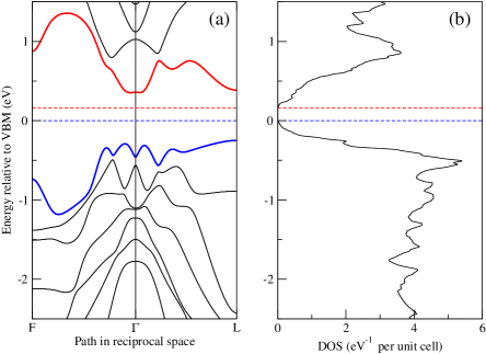
Figure 2: (a) LDA bandstructure of Bi₂Te₃ including spin-orbit coupling (SOC) calculated along F-$\Gamma$-L where F$=(0,0.5,0.5)$ and L$=(0,0.5,0)$ in units of the reciprocal lattice vectors. The last valence bands and first conduction bands are respectively colored in blue and red. (b) Density of states (DOS) per unit cell computed for a $256\times 256\times 256$ grid of kpoints with a gaussian smearing of 10 meV. In both pannels, the valence band maximum is set at zero and displayed as a blue dashed line while the conduction band minimum is displayed as a red dashed line. The conduction bands are shifted towards higher energies from 120 meV to mimic the self-energy corrections.

Indeed, the spin-orbit coupling (SOC) produces a band inversion in the vicinity of the $\Gamma$ point and shifts the band extremas from the high symmetry lines. Our calculated band extremas are found in the three mirror planes in agreement with other theoretical studiesluo_2012 ; wang_2007 ; kioupakis_2010 ; nechaev_2013 . As two extremas are found in each mirror plane, the multiplicity of our calculated extremas is 6 as suggested by Shubnikov-de Haas experimentskohler1_1976 ; kohler2_1976 and Landau level spectroscopymohelsky_2020 . The extremas of the valence band and conduction band in the $x=0$ mirror plane depicted in Fig. 3 are respectively found at $\pm(0.349,0.523,0.349)$ and $\pm(0.542,0.647,0.542)$ in units of the reciprocal lattice vectors while these extremas are respectively located at $\pm(0.37,0.54,0.37)$ and $\pm(0.58,0.68,0.58)$ in Ref. kioupakis_2010 .

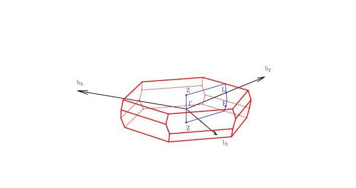
Figure 3: First Brillouin zone where the $x=0$ mirror plane (in blue) has been highlighted and where four high symetry ${\bf{k}}$-points, labelled $\Gamma$, $Z$, $L$ and $F$ are shown. The $x=0$ mirror plane is spanned by the reciprocal lattice vectors ${\bf{b}}_{2}$ ($\Gamma-L$ direction) and ${\bf{b}}_{1}+{\bf{b}}_{2}+{\bf{b}}_{3}$ ($\Gamma-Z$ direction) and the two other mirror planes (not shown) are obtained by applying $C_{3}$ rotations around the trigonal axis to the $x=0$ mirror plane.

Furthermore, the calculated LDA indirect gap is $\sim 42$ meV while the minimum direct gap is $\sim 91$ meV. The indirect gap differs from the LDA gap $\sim 87$ meV reported in Ref. kioupakis_2010 . Such a difference might be ascribed to the lattice cell parameters and/or internal coordinates that are expected to play a significant role on both the positions of the extremas and the values of the gapsnechaev_2013 . Optical measurements performed at 10 K led to a probably indirect band gap of $150\pm 20$ meVthomas_1992 and a direct gap of $220\pm 20$ meVthomas_1992 confirmed by more recent ellipsometry measurementsdubroka_2017 . The discrepancy between the theoretical and experimental results is noticeable and reflects the fact that the LDA eigenvalues can not be interpreted as quasiparticle energies. More sophisticated approaches based on the evaluation of the self-energy within the GW approximationhybertsen_1986 ; onida_2002 ; arnaud_2000 ; lebegue_2003 , are needed to provide a better description of quasiparticle properties. All the GW calculationskioupakis_2010 ; yazyev_2012 ; aguilera_2013 ; nechaev_2013 produce band gaps in better agreement with experiments. It’s worth highlighting that an accurate description of the quasiparticle bandstructure near the $\Gamma$ point necessitates to take into account the non diagonal elements of the self-energy operatoraguilera_2013 . The self-energy corrections, while less than 200 meV for one band and one kpointyazyev_2012 , are highly non trivial. Indeed, the rigid shift scissor approximation is not valid for the highest valence band and lowest conduction bandyazyev_2012 ; aguilera_2013 , especially in the vicinity of the $\Gamma$ point where the band inversion occurs and where the direct LDA band gaps are reducedaguilera_2013 . However, as this approximation seems to be well founded for other bands, we shift all conduction bands from 120 meV with respect to the valence bands to reproduce both the experimental indirect and direct gaps and keep in mind that we only achieve a poor description of the self-energy corrections needed to compute the optical properties beyond the standard random-phase approximation (RPA).

V OPTICAL PROPERTIES AT THE RPA LEVEL

Within the RPAadler_1962 ; wiser_1963 , the dielectric matrix for a given ${\bf q}$ wavevector reads:

$$\epsilon_{{\bf G},{\bf G}^{\prime}}({\bf q},\omega) = \delta_{{\bf G},{\bf G}^{\prime}}-\frac{e^{2}}{4\pi\epsilon_{0}}\frac{4\pi}{v|{\bf q}+{\bf G}||{\bf q}+{\bf G}^{\prime}|}\frac{1}{N}\sum_{{\bf k},n,m}\frac{f_{n,{\bf k}-{\bf q}}-f_{m,{\bf k}}}{\epsilon_{n{\bf k}-{\bf q}}-\epsilon_{m{\bf k}}+\hbar\omega+i\delta}$$ (4)

$$\times\langle n{\bf k}-{\bf q}|e^{-i({\bf q}+{\bf G}).{\bf r}}|m{\bf k}\rangle\langle m{\bf k}|e^{i({\bf q}+{\bf G}^{\prime}).{\bf r}}|n{\bf k}-{\bf q}\rangle$$

where $({\bf G},{\bf G}^{\prime})$ is a couple of reciprocal lattice vectors, $\epsilon_{m{\bf k}}$ are the Kohn-Sham energies for band $m$ and wave vector ${\bf k}$, $f_{m,{\bf k}}\equiv f(\epsilon_{m{\bf k}})$ are the occupation numbers within the Fermi-Dirac distribution $f$ at temperature $T$, $v$ is the unit cell volume and $N$ is the number of kpoints included in the summation. In this expression, the time dependence of the field was assumed to be $e^{-i\omega t}$ and the small positively defined constant $\delta$ guarantees that the matrix elements of $\epsilon(\omega)$ are analytic functions in the upper half plane. The macroscopic dielectric tensor $\overline{\overline{\epsilon}}(\omega)$ is a $3\times 3$ matrix given by:

$$\hat{{\bf q}}^{\top}~{}\overline{\overline{\epsilon}}(\omega)~{}\hat{{\bf q}}=1/\lim_{{\bf q}\to 0}\epsilon^{-1}_{{\bf{0}},{\bf{0}}}=\lim_{{\bf q}\to 0}\epsilon_{0,0}({\bf q},\omega)-\lim_{{\bf q}\to 0}\sum_{{\bf G},{\bf G}^{\prime}\neq{\bf{0}}}\epsilon_{0,{\bf G}}({\bf q},\omega)\epsilon^{-1}_{{\bf G},{\bf G}^{\prime}}({\bf q},\omega)\epsilon_{{\bf G}^{\prime},0}({\bf q},\omega),$$ (5)

where $\hat{{\bf q}}$ is a unitary vector along the wavevector ${\bf q}$. Neglecting the local field (LF) effects amounts to assuming that the dielectric matrix is diagonal, i.e. to neglecting the second term in Eq. 5. Given the hexagonal symmetry of Bi₂Te₃, $\overline{\overline{\epsilon}}(\omega)$ is diagonal with only two independent elements, namely $\epsilon_{\perp}(\omega)$ and $\epsilon_{\parallel}(\omega)$ that are respectively obtained for $\hat{{\bf q}}$ perpendicular and $\hat{{\bf q}}$ parallel to the trigonal axis. The dielectric matrix defined in Eq. 4 is computed with the YAMBO codeyambo_2009 ; yambo_2019 which requires the ground state electronic structure computed with the ABINIT codegonze_2009 ; gonze_2016 . Indeed, the Kohn-Sham eigenvalues $\epsilon_{m{\bf k}}$ and eigenvectors $|m{\bf{k}}\rangle$ are key ingredients to compute the dielectric function at the RPA level. From a practical point of view, we used a $64\times 64\times 64$ kpoints grid (22913 irreducible kpoints) and included 28 valence bands and 34 conduction bands in our calculations to converge the dielectric function without LF effects. The LF effects are included by taking into account the second term in Eq. 5, where a $302\times 302$ body matrix $\epsilon_{{\bf G},{\bf G}^{\prime}}({\bf q}\to{\bf{0}},\omega)$ with ${\bf G},{\bf G}^{\prime}\neq{\bf{0}}$, ensures the convergence of the macroscopic dielectric function.

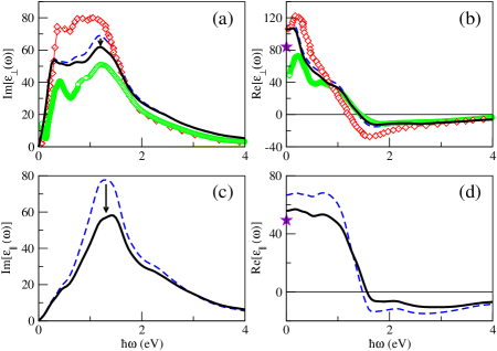
Figure 4: Imaginary and real part of the dielectric function of Bi₂Te₃ computed at the RPA level with LF effects (thick black lines) and without LF effects (blue dashed lines) for an electric field perpendicular to the trigonal axis (upper pannels) and parallel to the trigonal axis (lower pannels) as a function of the photon energy $\hbar\omega$ (in eV). All the conduction bands have been shifted from 120 meV with respect to the valence bands in order to roughly reproduce the self-energy corrections. The imaginary and real part of the dielectric function obtained from ellipsometry measurementsdubroka_2017 and from a Kramers Kronig analysis of reflectivity measurementsGreenaway_1965 are respectively displayed as green circles and red diamonds in the upper pannels. The two vertical arrows in pannels (a) and (c) show how the imaginary part of the dielectric function evolves when LF effects are included. The stars in pannel (b) and (d) denote the experimental clamped-nuclei static dielectric constants extracted from the IR reflectance spectras measured at 300 Krichter_1977 .

Both the imaginary part and the real part of the dielectric function $\epsilon_{\perp,\parallel}(\omega)$ computed with LF effects (thick black lines) and without LF effects (blue dashed lines) at $T=300$ K are displayed in Fig. 4 and compared to the experimental resultsdubroka_2017 ; Greenaway_1965 shown as circles and diamonds in the upper pannels of Fig. 4. The imaginary part of the dielectric function computed without LF effects for an electric field ${\bf{E}}\perp{\bf{c}}$ (see Fig. 4(a)) displays two peaks respectively located at 0.32 eV and 1.21 eV while the experimental peaksdubroka_2017 are respectively located at 0.42 eV and 1.22 eV. Such a difference might be related to our crude implementation of the self-energy corrections (the conduction bands have been shifted from 120 meV with respect to the valence bands) or to excitonic effects neglected at our level of approximationonida_2002 ; arnaud_2001 ; arnaud_2006 . It’s important to point out that the peak located at $0.32$ eV is sensitive to the temperature $T$ and disappears at $T=300$ K when the conduction bands are not shifted, which can be explained by the unphysical thermal excitation of electrons from the highest valence band to the lowest conduction band arising from the tiny indirect band gap $\sim 42$ meV at the LDA level. We also observe that the LF effects do not affect the positions of the peaks but slightly reduce the intensity of the peak located at 1.21 eV. The situation is clearly different for ${\bf{E}}\parallel{\bf{c}}$ (see Fig. 4(c)). Indeed, the imaginary part of the dielectric function computed without LF effects displays one peak located at 1.31 eV which is shifted to 1.43 eV when LF effects are included. Furthermore, the intensity of this peak is decreased by $\sim 25$ % when LF effects are included, suggesting that LF effects are crucial to predict the optical properties for ${\bf{E}}\parallel{\bf{c}}$. This observation is somehow expected as the LF effects, vanishing for an homogeneous electron gas, are as large as the degree of inhomogeneity in the charge density increasesarnaud_2001 . Indeed, the inhomogeneity in the charge density is undeniably strong along the trigonal axis, namely the stacking axis of the quintuple layers.

We observe a discrepancy between theory and experiment as our calculated imaginary part of the dielectric function for ${\bf{E}}\perp{\bf{c}}$ (see Fig. 4(a)) falls in between the two experimental resultsdubroka_2017 ; Greenaway_1965 . Importantly, the two experimental results only coincide above 3 eV, where the anisotropy in the optical response starts to be negligible as shown in our calculations with or without LF effects. The experimental results of Ref.Greenaway_1965 are deduced from a Kramers-Kronig (KK) transformation of the near-normal incidence reflectivity spectra for ${\bf{E}}\perp{\bf{c}}$. Thus, both the real and imaginary part of the dielectric function might be erroneous because they are very sensitive to small errors in the reflectivity data and in the high energy extrapolation. The experimental results obtained from ellipsometry measurementsdubroka_2017 might also be in error as the authors assumed that they only probe the in-plane component of the dielectric function ($\epsilon_{\perp}$) in the oblique geometry of their measurements while they also probed the out of plane component of the dielectric function ($\epsilon_{\parallel}$), introducing some errors in the determination of $\epsilon_{\perp}$ as our calculations show that the anisotropy in the optical response up to 3 eV is far from being negligible. Therefore, it’s difficult to draw a definitive conclusion as two measurements do not lead to the same results, highlighting the need for new experimental studies. It’s also important to point out that excitonic effects, neglected at the RPA level, might change the calculated dielectric function. However, excitonic effects are expected to be small because of the large dielectric screening. Indeed, our clamped-nuclei static dielectric constants $\epsilon_{\infty,\perp}$ and $\epsilon_{\infty,\parallel}$ with (without) LF effects are respectively equal to 105 (110) and 56 (67), while the experimental static dielectric constants infered from infrared spectroscopy measurementsrichter_1977 and shown as stars in Fig. 4(b) and 4(d), are respectively equal to 85 and 50. Such a large contribution of the electrons to the static dielectric constants can be understood from the Kramers Kronig transformation that relates the real part of the dielectric function to the imaginary part of the dielectric function. Indeed, we have

$$\epsilon_{\infty,\perp,\parallel}=\frac{2}{\pi}\int_{0}^{\infty}d\omega~{}\frac{\textrm{Im}\left[\epsilon_{\perp,\parallel}(\omega)\right]}{\omega}.$$ (6)

As $\textrm{Im}\left[\epsilon_{\perp}(\omega)\right]>\textrm{Im}\left[\epsilon_{\parallel}(\omega)\right]$ for $\hbar\omega$ below 1.4 eV , we can conclude that $\epsilon_{\infty,\perp}>\epsilon_{\infty,\parallel}$ since the anisotropy in the optical response is weak above 1.4 eV when LF effects are included. Furthermore, $\epsilon_{\infty,\perp}$ and $\epsilon_{\infty,\parallel}$ are very large because of strong interband transitions starting from 210 meV (direct LDA band gap increased from 120 meV) that strongly contribute to the static dielectric constant because of the $1/\omega$ weighting factor in the integrand of Eq. 6.

Interestingly, as shown in Fig. 4(b) and Fig. 4(d), the real part of $\epsilon_{\perp}$ ($\epsilon_{\parallel}$) including LF effects crosses the zero axis around 1.42 eV (1.56 eV) and becomes negative up to 6 eV. Thus, plasmonic applications, as nicely demonstrated in Ref.zhao_2015 , can be envisionned but with the inconvenient that the imaginary part of the dielectric function is far from being negligible in this spectral range, especially in the visible range. Our calculations also show that Bi₂Te₃ behaves as an hyperbolic material in a very narrow range of energy between 1.42 and 1.56 eV where the permittivity components in different directions have opposite sign ($\epsilon_{\perp}\cdot\epsilon_{\parallel}<0$). Therefore, our theoretical results contradict the ellipsometry measurements of Ref.esslinger_2014 , where the authors claimed that Bi₂Te₃ is a natural hyperbolic material in the visible range. Such a discrepancy might be ascribed to the fact that the real part of the dielectric function for ${\bf{E}}\parallel{\bf{c}}$ is incorrectly measured.

We also computed the normal incidence reflectivity according to

$$R_{\perp,\parallel}(\omega)=\left|\frac{n_{\perp,\parallel}(\omega)-1}{n_{\perp,\parallel}(\omega)+1}\right|^{2},$$ (7)

where $n_{\perp,\parallel}(\omega)=\sqrt{\epsilon_{\perp,\parallel}(\omega)}$ is the optical index calculated with or without LF effects for $\mathbf{E}\perp\mathbf{c}$ or $\mathbf{E}\parallel\mathbf{c}$.

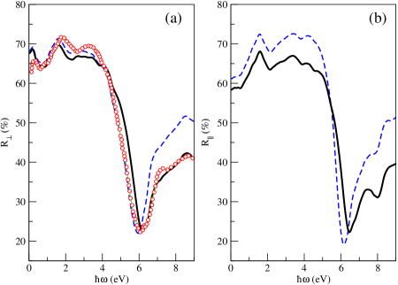
Figure 5: Computed optical reflectivity with (thick black lines) and without (thin blue dashed lines) LF effects for $\mathbf{E}\perp\mathbf{c}$ (left pannel) and $\mathbf{E}\parallel\mathbf{c}$ (right pannel) compared to the near-normal incidence reflectance spectra (open circles) measured at 300 K for $\mathbf{E}\perp\mathbf{c}$Greenaway_1965 .

As shown in Fig. 5(a), the overall agreement between theory and experimentGreenaway_1965 for $\mathbf{E}\perp\mathbf{c}$ is fairly good when LF effects are included. It’s worth remarking that LF effects do not change the reflectivity spectra very much between 0 eV and 4 eV as can be inferred from Fig. 4(a) and Fig. 4(b) but lead to a strong decrease of the calculated reflectivity from 6 to 9 eV bringing the calculated spectra in closer agreement with the experimental spectraGreenaway_1965 . The situation is more contrasted for $\mathbf{E}\parallel\mathbf{c}$ as LF effects are noticeable everywhere. As shown in Fig. 5(b), the calculated reflectivity with LF effects is much smaller than the calculated reflectivity without LF effects almost everywhere up to 9 eV, except for a narrow range of energy between 5.5 eV and 6.4 eV, where the reflectivity displays a dip.

VI FREQUENCIES AT THE ZONE CENTER

As the primitive cell contains five atoms, there are 15 lattice dynamical modes at the Brillouin zone center, three of which are acoustic modes. Group theory classifies the remaining 12 optical modes into 2 A_1g (R), 2 E_g (R), 2 A_2u (IR) and 2 E_u (IR) modes, where R and IR refer to Raman and infrared active modes respectively. We computed the zone center frequencies within a DFPT approachgonze_1997 for the experimental structure at 300 Kfrancombe_1958 , where only the internal coordinates have been relaxed (see table 1).

Table 2: Experimental and theoretical values of Raman and infrared phonon frequencies for Bi₂Te₃ in units of cm^-1. Experimental Ramanrichter_1977 ; wang_2013 and infrared valuesrichter_1977 were measured at 300 K. The values within parentheses correspond to the frequencies in THz and the most recent experimental resultswang_2013 are underlined.

Symmetry	Experiment		Theory
E${}_{g}^{1}$	-	37 (1.11)	36.81 (1.10)
A${}_{1g}^{1}$	62.5 (1.87)	62 (1.86)	57.25 (1.71)
E${}_{g}^{2}$	103 (3.09)	102 (3.06)	97.96 (2.93)
A${}_{1g}^{2}$	134 (4.02)	135 (4.05)	129.25 (3.87)
E${}_{u}^{1}$	$50\pm 2$ (1.50 $\pm 0.06$)		54.25 (1.62)
A${}_{2u}^{1}$	$94\pm 4$ (2.82 $\pm 0.12$)		93.23 (2.79)
E${}_{u}^{2}$	$95\pm 5$ (2.85 $\pm 0.15$)		91.75 (2.75)
A${}_{2u}^{2}$	$120\pm 5$ (3.60 $\pm 0.15$)		120.25 (3.60)

As shown in Table 2, the overall agreement between theory and experimentrichter_1977 ; wang_2013 is satisfactorily and the largest discrepancy occurs for the A${}_{1g}^{1}$ and E${}_{u}^{1}$ frequencies that are respectively underestimated and overestimated from 8% with respect to the experimental frequencies. Such a difference might be ascribed to anharmonic effects not captured in our calculationsyang_2020 .

VII BORN EFFECTIVE CHARGES

We used a finite electric field approachsouza_2002 in order to compute the Born effective charge tensors. The force along $\beta$ acting on atom $p$ reads

$$F_{p}^{\beta}=e\sum_{\alpha}Z^{*}_{p,\alpha,\beta}E^{\alpha},$$ (8)

where $E^{\alpha}$ is the component along $\alpha$ of the macroscopic electric field and $Z^{*}_{p,\alpha,\beta}$ is the Born effective charge tensor defined for each atom $p$. Given the hexagonal symmetry of Bi₂Te₃, the tensor is diagonal and reduces to two values $Z^{*}_{p,\perp}=Z^{*}_{p,1,1}=Z^{*}_{p,2,2}$ and $Z^{*}_{p,\parallel}=Z^{*}_{p,3,3}$ for each atom. Using Eq. 8, we conclude that

$$\left\{\begin{array}[]{ll}F_{p}^{\beta}=Z^{*}_{p,\perp}E^{\beta}&~{}\textrm{when}~{}\beta=1,2\\ F_{p}^{\beta}=Z^{*}_{p,\parallel}E^{\beta}&~{}\textrm{when}~{}\beta=3\\ \end{array}\right.$$ (9)

Thus, we computed the forces acting on each atom for an electric field perpendicular and parallel to the trigonal axis whose amplitude is varied from $-10^{-6}$ a.u to $10^{-6}$ with a step of $0.5\times 10^{-6}$ a.u (2.57 kV.cm^-1).

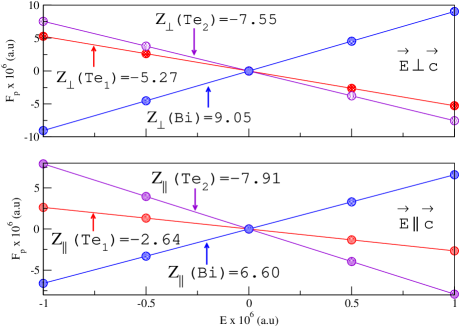
Figure 6: Forces $F_{p}$ (in a.u) as a function of the macroscopic electric field $E$ (in a.u) applied perpendicular (upper pannel) and parallel (lower pannel) to the trigonal axis for the experimental structure at 300 Kfrancombe_1958 .

As shown in Fig. 6, the forces $F_{p}$ acting on each atom $p$ vary linearly with the amplitude of the macroscopic electric field $E$. A linear fitting provides the Born effective charges that are gathered in table 3.

Table 3: Calculated Born effective charges for the two equivalent Bi atoms, the two equivalent Te₁ atoms and the Te₂ atom underlying the five-point basis. The degree of anisotropy in the Born effective charges is quantified by Z${}_{\parallel}^{*}/$Z${}_{\perp}^{*}$.

	Bi	Te1	Te2
Z${}_{\parallel}^{*}$	6.60	-2.64	-7.91
Z${}_{\perp}^{*}$	9.05	-5.27	-7.55
Z${}_{\parallel}^{*}/$Z${}_{\perp}^{*}$	0.729	0.500	1.047

It’s worth pointing out that the acoustic sum rule $\sum_{p}Z^{*}_{p,\perp~{}\textrm{or}~{}\parallel}$ is fulfilled to within $10^{-5}$ suggesting that our calculations are well converged. The effective charges are large and differ strongly from what can be expected for fully ionic configurations corresponding to closed shell ions ($+3$ for Bi and $-2$ for Te). However, it’s worth reminding that effective charges are dynamic only and reflect the effect of covalencylee_2003 . Interestingly, the Born effective charges have surprisingly different values for the Te₁ and Te₂ atoms and show large anisotropy for the Te₁ atoms that form strongly covalent bonds with the Bi atoms as the distance between the Te₁ and Bi atoms is the shortest one. The Born effective charges of Bi atoms also display some degree of anisotropy. From a physical point of view, the two Bi atoms and the two Te₁ atoms behave respectively as anisotropic cations and anions, while the Te₂ atom behaves as an isotropic anion.

VIII INFRARED DIELECTRIC TENSOR

We consider a unit cell of volume $v$ containing $n$ atoms. The total energy of the unit cell $E_{tot}$, when a macroscopic electric field $\bf{E}$ is applied, can be taylor expanded as:

$$E_{tot}=E_{0}+\frac{1}{2}\sum_{p,p^{\prime},\alpha,\alpha^{\prime}}u_{p}^{\alpha}\frac{\partial^{2}E_{tot}}{\partial u_{p}^{\alpha}\partial u_{p^{\prime}}^{\alpha^{\prime}}}u_{p^{\prime}}^{\alpha^{\prime}}+\sum_{p,\alpha,\beta}\frac{\partial^{2}E_{tot}}{\partial u_{p}^{\alpha}\partial E^{\beta}}u_{p}^{\alpha}E^{\beta}+\frac{1}{2}\sum_{\alpha,\beta}\frac{\partial^{2}E_{tot}}{\partial E^{\alpha}\partial E^{\beta}}E^{\alpha}E^{\beta},$$ (10)

where $u_{p}^{\alpha}$ is the displacement of atom $p$ ($p\in\{1,\cdots,n\}$) along the direction $\alpha$ and $E^{\beta}$ the component of the macroscopic field along $\beta$ with $\alpha,\beta\in\{1,2,3\}$. We can introduce the elastic constants $C_{p,p^{\prime}}^{\alpha,\alpha^{\prime}}$, the dimensionless Born effective charge tensor $Z^{*}_{p,\beta,\alpha}$ and the dimensionless electronic tensor susceptibility $\chi_{\alpha,\beta}$, respectively defined by

$$C_{p,p^{\prime}}^{\alpha,\alpha^{\prime}}=\frac{\partial^{2}E_{tot}}{\partial u_{p}^{\alpha}\partial u_{p^{\prime}}^{\alpha^{\prime}}},~{}Z^{*}_{p,\beta,\alpha}=-\frac{1}{e}\frac{\partial^{2}E_{tot}}{\partial u_{p}^{\alpha}\partial E^{\beta}},~{}\textrm{and}~{}\chi_{\alpha,\beta}=-\frac{1}{v\epsilon_{0}}\frac{\partial^{2}E_{tot}}{\partial E^{\alpha}\partial E^{\beta}}.$$ (11)

Thus, the total energy reads

$$E_{tot}=E_{0}+\frac{1}{2}\sum_{p,p^{\prime},\alpha,\alpha^{\prime}}u_{p}^{\alpha}C_{p,p^{\prime}}^{\alpha,\alpha^{\prime}}u_{p^{\prime}}^{\alpha^{\prime}}-e\sum_{p,\alpha,\beta}Z^{*}_{p,\beta,\alpha}u_{p}^{\alpha}E^{\beta}-\frac{1}{2}v\epsilon_{0}\sum_{\alpha,\beta}\chi_{\alpha,\beta}E^{\alpha}E^{\beta},$$ (12)

leading to a force (See Eq. 8) exerted on atom $p$ by the macroscopic elecric field when the atoms are held at their equilibrium position. From Eq. 12, we get the component along $\beta$ of the polarization

$$P^{\beta}=-\frac{1}{v}\frac{\partial E_{tot}}{\partial E^{\beta}}=P^{\beta,ion}+P^{\beta,el},$$ (13)

where the ionic contribution to the polarization reads

$$P^{\beta,ion}=\frac{e}{v}\sum_{\alpha,p}Z^{*}_{p,\beta,\alpha}u_{p}^{\alpha},$$ (14)

and the electronic contribution reads

$$P^{\beta,el}=\epsilon_{0}\sum_{\alpha}\chi_{\beta,\alpha}E^{\alpha}.$$ (15)

Using Eq. 12, the equation of motion for atom $p$ of mass $M_{p}$ reads

$$M_{p}\ddot{u}_{p}^{\alpha}=-\frac{\partial E_{tot}}{\partial u_{p}^{\alpha}}=-\sum_{p^{\prime},\alpha^{\prime}}C_{p,p^{\prime}}^{\alpha,\alpha^{\prime}}u_{p^{\prime}}^{\alpha^{\prime}}+e\sum_{\beta}Z^{*}_{p,\beta,\alpha}E^{\beta}.$$ (16)

When $\mathbf{E}=\mathbf{0}$, we can plug

$$u_{p}^{\alpha}=\sqrt{\frac{M}{M_{p}}}\epsilon_{p}^{\alpha}\exp[-i\omega t],$$ (17)

where $M=\sum_{p}M_{p}$, in Eq. 16 and solve the following eigenvalue problem

$$\sum_{p^{\prime},\alpha^{\prime}}D_{p,p^{\prime}}^{\alpha,\alpha^{\prime}}\epsilon_{p^{\prime}}^{\alpha^{\prime}}(\lambda)=\omega_{\lambda}^{2}\epsilon_{p}^{\alpha}(\lambda),$$ (18)

where $D_{p,p^{\prime}}^{\alpha,\alpha^{\prime}}=C_{p,p^{\prime}}^{\alpha,\alpha^{\prime}}/\sqrt{M_{p}M_{p^{\prime}}}$ is the dynamical matrix at the zone center. Here $\omega_{\lambda}$ and $\epsilon_{p}^{\alpha}(\lambda)$ are respectively the frequency and the displacement of atom $p$ along $\alpha$ for the mode $\lambda$, where $\lambda\in\{1,\cdots,3n\}$. The eigenvectors of Eq. 18 satisfy the orthogonality relations

$$\sum_{p,\alpha}\epsilon_{p}^{\alpha}(\lambda)\epsilon_{p}^{\alpha}(\lambda^{\prime})=\delta_{\lambda,\lambda^{\prime}}\Longleftrightarrow\mathbf{\epsilon}(\lambda)^{\top}\mathbf{\epsilon}(\lambda^{\prime})=\delta_{\lambda,\lambda^{\prime}},$$ (19)

since the zone center dynamical matrix is real and symmetric.

When $\mathbf{E}=\mathbf{E}_{0}\exp(-i\omega t)$, where $\omega$ is the frequency of the electric field in the THz range, we can plug

$$u_{p}^{\alpha}=\sqrt{\frac{M}{M_{p}}}z_{p}^{\alpha}\exp[-i\omega t],$$ (20)

into Eq. 16. Thereby, the following equation

$$\omega^{2}z_{p}^{\alpha}=\sum_{p^{\prime},\alpha^{\prime}}D_{p,p^{\prime}}^{\alpha,\alpha^{\prime}}z_{p^{\prime}}^{\alpha^{\prime}}-\frac{e}{\sqrt{MM_{p}}}\sum_{\beta}Z^{*}_{p,\beta,\alpha}E_{0}^{\beta}$$ (21)

must be solved. As $\{\mathbf{\epsilon}(\lambda),\lambda=1,\cdots,3n\}$ forms a complete basis set, we can seek a solution in the form

$$z_{p}^{\alpha}=\sum_{\lambda}A(\lambda)\epsilon_{p}^{\alpha}(\lambda),$$ (22)

where the coefficients $A(\lambda)$ have to be determined. Introducing Eq. 22 in Eq. 21 and using Eq. 18 leads to

$$\sum_{\lambda^{\prime}}A(\lambda^{\prime})\left[\omega^{2}-\omega_{\lambda^{\prime}}^{2}\right]\epsilon_{p}^{\alpha}(\lambda^{\prime})=-\frac{e}{\sqrt{MM_{p}}}\sum_{\beta}Z^{*}_{p,\beta,\alpha}E_{0}^{\beta}$$ (23)

By multiplying this identity with $\epsilon_{p}^{\alpha}(\lambda)$, summing over $p$ and $\alpha$ and using the orthogonality relation (Eq. 19), we obtain

$$A(\lambda)=-\frac{e}{M}\frac{1}{\omega^{2}-\omega_{\lambda}^{2}}\sum_{\beta^{\prime}}Z_{\beta^{\prime}}(\lambda)E_{0}^{\beta^{\prime}},$$ (24)

where the mode effective charge

$$Z_{\beta}(\lambda)=\sum_{p,\alpha}\sqrt{\frac{M}{M_{p}}}\epsilon_{p}^{\alpha}(\lambda)Z^{*}_{p,\beta,\alpha},$$ (25)

is a dimensionless quantity. Plugging Eq. 24 in Eq. 22, and using the definition of ionic polarization (Eq. 14) as well as Eq. 20, we obtain

$$P^{\beta,ion}(\omega)=\frac{e^{2}}{v}\frac{1}{M}\sum_{\beta^{\prime},\lambda}\frac{Z_{\beta}(\lambda)Z_{\beta^{\prime}}(\lambda)}{\omega_{\lambda}^{2}-\omega^{2}}E^{\beta^{\prime}}$$ (26)

By analogy with the definition of the electronic susceptibility (Eq. 15), we can define an ionic susceptibility

$$\chi^{ion}_{\beta,\beta^{\prime}}(\omega)=\frac{e^{2}}{\epsilon_{0}v}\frac{1}{M}\sum_{\lambda}\frac{S_{\beta,\beta^{\prime}}(\lambda)}{\omega_{\lambda}^{2}-\omega^{2}-2i\omega\gamma_{\lambda}},$$ (27)

where $2\gamma_{\lambda}$ is the full width at half maximum (FWHM) of the phonon peak and $S_{\beta,\beta^{\prime}}(\lambda)=Z_{\beta}(\lambda)Z_{\beta^{\prime}}(\lambda)$ is a dimensionless $3\times 3$ real symmetric matrix. It’s straightforward to show using Eq. 25 that this matrix $S$ is zero for a gerade mode. Interestingly, $S$ might be non diagonal for degenerated modes like the $E_{u}^{1}$ mode at 1.62 THz or the $E_{u}^{2}$ mode at 2.75 THz that can couple to an electric field perpendicular to the trigonal axis. However, the matrix $S$ becomes diagonal when the polarization of the first $E_{u}$ mode is chosen along one of the two fold axis (x-axis) while the polarization of the second $E_{u}$ mode lies along one of the mirror plane (y-axis). Thus, we get:

$$\chi^{ion}_{\perp,\parallel}(\nu)=\frac{e^{2}}{4\pi^{2}\epsilon_{0}v}\frac{1}{M}\sum_{\lambda}\frac{S_{\perp,\parallel}(\lambda)}{\nu_{\lambda}^{2}-\nu^{2}-i\nu\gamma_{\lambda}/\pi},$$ (28)

where $S_{\perp}(\lambda)=\left[Z_{1}(\lambda)\right]^{2}~{}\textrm{or}~{}\left[Z_{2}(\lambda)\right]^{2}$, $S_{\parallel}(\lambda)=\left[Z_{3}(\lambda)\right]^{2}$ (see Eq. 25) and where the summation can be restricted to the IR active modes.

Table 4: Frequencies (in THz), oscillator strengths (dimensionless quantities) and normalized atomic displacements (see Eq. 19) for the IR active modes. The calculations have been done for the experimental lattice structurefrancombe_1958 using the values of the Born effective charges reported in table 3.

Symmetry	Frequency	Oscillator strengths		Normalized atomic displacements					Direction
		$S_{\perp}$	$S_{\parallel}$	Te1	Bi	Te2	Bi	Te1
E${}_{u}^{1}$	1.62	1318.15	-	0.310	-0.475	0.596	-0.475	0.310	$x$, $y$
E${}_{u}^{2}$	2.75	15.48	-	0.494	-0.114	-0.696	-0.114	0.494	$x$, $y$
A${}_{2u}^{1}$	2.79	-	540.46	0.122	0.262	-0.913	0.262	0.122	$z$
A${}_{2u}^{2}$	3.60	-	273.73	0.571	-0.413	-0.085	-0.413	0.571	$z$

The oscillator strengths $S_{\perp}$ and $S_{\parallel}$ for an electric field respectively perpendicular and parallel to the trigonal axis are reported in table 4. We have previously seen that the oscillator strengths are related to both the eigenvectors of the zone center dynamical matrix and the mode effective charges (See Eq. 25). The huge difference between the oscillator strength for the $E_{u}^{1}$ and $E_{u}^{2}$ modes arises from the fact that all atoms contribute to $S_{\perp}$ for the $E_{u}^{1}$ mode while only the Bi atoms contribute significantly for the $E_{u}^{2}$ mode. Indeed, the displacements of atoms have the same sign for both modes with the exception of the Te₂ atom whose displacement along the $E_{u}^{2}$ mode is reversed, producing an almost complete cancellation of the Te atoms to $S_{\perp}$.

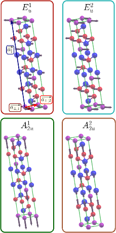
Figure 7: Displacements of the atoms for the two $E_{u}$ modes polarized along the $x$-axis and for the two $A_{2u}$ modes polarized along the $z$-axis (trigonal axis). The Te₁, Te₂ and Bi atoms are respectively colored in red, purple and blue.

For the sake of completeness, the displacements of atoms inside the hexagonal unit cell for the four different IR active modes are depicted in Fig. 7.

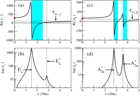
Figure 8: Imaginary and real part of the IR dielectric function of Bi₂Te₃ computed with Eq. 28 for an electric field perpendicular to the trigonal axis (pannels a and b) and parallel to the trigonal axis (pannels c and d) as a function of frequency $\nu$ (in THz). We assumed that $\gamma_{\lambda}=0.44$ THz for the $E_{u}$ modes and that $\gamma_{\lambda}=0.22$ THz for the $A_{2u}$ modes. Note that the frequencies of both $E_{u}$ modes have been slightly renormalized to match the experimental frequenciesrichter_1977 reported in table 2 while the theoretical frequencies of both $A_{2u}$ modes have been considered. The stars in pannel (a) and (c) denote the experimental static dielectric constants extracted from the IR reflectance spectras measured at 15 Krichter_1977 and the colored domain in pannel (a) delimits the Restrahlen band of the $E_{u}^{1}$ mode situated between the transversal optical frequency at 1.5 THz and the longitudinal optical frequency at 2.49 THz while the two colored domains in pannel (c) delimit the Restrahlen bands of the $A_{2u}^{1}$ ($A_{2u}^{2}$) mode situated between the transversal optical frequency at 2.79 THz (3.60 THz) and the longitudinal optical frequency at 3.14 THz (3.95 THz).

The IR dielectric constant is defined as

$$\epsilon_{\perp,\parallel}(\nu)=\epsilon_{\infty,\perp,\parallel}+\chi^{ion}_{\perp,\parallel}(\nu),$$ (29)

where the electronic contribution to the static dielectric function at the RPA level denoted as $\epsilon_{\infty,\perp,\parallel}$, also named clamped-nuclei dielectric constant, can be approximated as a constant for frequencies less than 5 THz. Fig. 8(a) and 8(c) display the real part of the IR dielectric function computed for an electric field perpendicular (${\bf{E}}\perp{\bf{c}}$) and parallel (${\bf{E}}\parallel{\bf{c}}$) to the trigonal axis. The two $E_{u}$ modes can be driven for ${\bf{E}}\perp{\bf{c}}$ while the two $A_{u}$ modes can be driven for ${\bf{E}}\parallel{\bf{c}}$. The real part changes sign each time the frequency $\nu$ crosses the frequency of an IR active mode depicted as a vertical dashed line in Fig. 8. The only exception concerns the mode $E_{u}^{2}$ whose oscillator strength is very weak (see Table 4). Interestingly, our calculations reproduce the static dielectric functions denoted as stars for both polarizations. The ionic and electronic contributions to the total susceptibility are respectively $\sim$ 192 and $\sim$ 104 ($\sim$ 29 and $\sim$ 55) for ${\bf{E}}\perp{\bf{c}}$ (${\bf{E}}\parallel{\bf{c}}$), reflecting the high degree of anisotropy of the optical properties in the THz range. It’s worth outlining that $\textrm{Re}[\epsilon_{\perp}].\textrm{Re}[\epsilon_{\parallel}]<0$ for the three Restrahlen bands depicted as vertical colored domains in Fig. 8. Hence, Bi₂Te₃ as h-BNCaldwell_2014 or $\alpha$-MoO$3$Ma_2018 exhibits natural hyperbolicity and might support hyperbolic phonon-polaritons. We also note that the imaginary part of the IR dielectric function displayed in Fig. 8(b) and 8(d) has a lorentzian profile in the vicinity of each resonance with a full width at half maximum (FHWM) given by $\gamma_{\lambda}/\pi$ and remind that the phonon lifetime is given by $1/\gamma_{\lambda}$. Here, we assumed that the lifetimes of both $E_{u}$ modes is $\sim 2.27$ ps while the lifetimes of both $A_{u}$ modes is $\sim 4.54$ ps to best reproduce the IR reflectance spectras discussed in the following section.

IX INFRARED REFLECTIVITY SPECTRUM

The normal incidence reflectivity spectras computed according to Eq. 7 for ${\bf{E}}\perp{\bf{c}}$ and ${\bf{E}}\parallel{\bf{c}}$ are compared to the experimental spectras at 15 Krichter_1977 in Fig. 9.

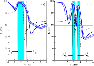
Figure 9: Computed IR reflectivity spectras with (thick lines) and without (dashed lines) the free electron contribution for ${\bf{E}}\perp{\bf{c}}$ (left pannel) and ${\bf{E}}\parallel{\bf{c}}$ (right pannel) compared to the experimental spectras (open circles) recorded at 15 Krichter_1977 . The restrahlen bands are depicted as colored domains and the horizontal lines correspond to the expected value of the reflectivity well above the highest IR frequency ($\sim 3.6$ THz) but below the band gap frequency ($\sim 51$ THz).

Roughly speaking, the overall agreement between the calculated reflectivity (dashed lines) and the experimental reflectivity (open circles) for both polarizations is fairly good within the Restrahlen bands, while poor outside, suggesting that the free electrons arising from doping contribute to the dielectric function. Hence, we consider the dielectric function

$$\overline{\epsilon}_{\perp,\parallel}(\nu)=\epsilon_{\perp,\parallel}(\nu)-\nu_{pl,\perp,\parallel}^{2}/\nu(\nu+i\gamma_{\perp,\parallel}),$$ (30)

where $\epsilon_{\perp,\parallel}$ is defined in Eq. 29 and where the charge carrier contribution depends on two parameters, namely the plasmon frequency $\nu_{pl,\perp,\parallel}$ and plasmon damping $\gamma_{\perp,\parallel}$. The calculated reflectivity shown as a solid line in Fig. 9 for ${\bf{E}}\perp{\bf{c}}$ (${\bf{E}}\parallel{\bf{c}}$) with $\nu_{pl,\perp}\sim 26.6$ THz ($\nu_{pl,\parallel}\sim 24.2$ THz) reproduces nicely the experimental reflectivity provided that the plasmon damping constant $\gamma_{\perp}$ ($\gamma_{\parallel}$) is well chosen. We found that a constant plasmon damping $\gamma_{\perp}\sim 0.95$ THz allows to reproduce the experimental reflectivity spectra for ${\bf{E}}\perp{\bf{c}}$ while a frequency dependent plasmon damping $\gamma_{\parallel}$ is crucial to reproduce the reflectivity spectra for ${\bf{E}}\parallel{\bf{c}}$. Hence, we considered the following formula:

$$\gamma_{\parallel}(\nu)=\frac{\gamma_{l}+\gamma_{h}}{2}+\frac{\gamma_{h}-\gamma_{l}}{2}\tanh\left(\frac{\nu-\nu_{0}}{\Delta\nu}\right),$$ (31)

to interpolate between the low frequency value of the plasmon damping denoted as $\gamma_{l}\sim 0.24$ THz and the high frequency value, denoted as $\gamma_{h}\sim 1.7$ THz with a fairly steep variation in a frequency interval $2\Delta\nu\sim$ 1.4 THz centered on $\nu_{0}\sim 2.3$ THz.

X PLASMON FREQUENCIES

As shown in the previous part, the Drude contribution to the IR reflectivity can not be ignored. Indeed, a bulk charge carrier contribution originates from intrinsic defects, such as anion vacancies and antisite defects that are ubiquitous in most compound semiconductorsChuang_2018 . For instance, focusing on the latter, either a Te₁ atom can be replaced by a Bi atom, leading to hole charge carriers or a Bi atom can be replaced by a Te atom, leading to electron charge carriers. From an experimental point of view, the p-type or n-type charge carrier concentration can range from $3\times 10^{17}$ to $5\times 10^{19}$ cm^-3, depending on the growth conditions.

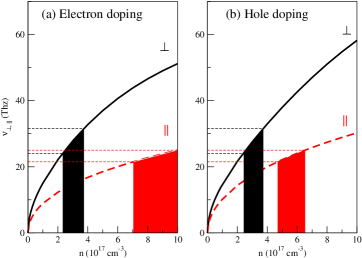
Figure 10: Plasmon frequencies $\nu_{pl,\perp}$ and $\nu_{pl,\parallel}$ (in THz) computed as a function of electron doping (left pannel) and hole doping (right pannel) up to $n=10^{18}$ cm^-3. The horizontal dashed lines of the same color span the range of plasmon frequencies that gives a good fitting of the reflectivity spectras shown in Fig. 9. The range of doping corresponding to the range of $\nu_{pl,\perp}$ ($\nu_{pl,\parallel}$) is depicted in black (red). The plasmon frequencies, that are hard to converge, are computed using a very dense $256\times 256\times 256$ grid of kpoints for a temperature $T\sim 15$ K.

Assuming that the rigid band model is valid, the plasma frequencies can be evaluated by tuning the Fermi level to achieve either electron or hole doping. In such a case, it is straightforward to show that the intraband contribution to the dielectric tensor defined in Eq. 5 behaves as $-\overline{\overline{\omega_{pl}^{2}}}/\omega^{2}$ where:

$$\omega_{pl,\alpha,\beta}^{2}=\frac{e^{2}}{4\pi\epsilon_{0}}\frac{4\pi}{v}\frac{1}{N}\sum_{{\bf k},n}v_{n{\bf k}}^{\alpha}v_{n{\bf k}}^{\beta}\left(-\frac{\partial f}{\partial\epsilon}\right)_{\epsilon_{n{\bf k}}}.$$ (32)

Here ${\bf v}_{n{\bf k}}\equiv\nabla_{\bf k}\epsilon_{n{\bf k}}/\hbar$ are the band velocities. It is important to note that only states at the Fermi level contribute to $\omega_{pl,\alpha,\beta}^{2}$ at $T=0$ since $-\frac{\partial f}{\partial\epsilon}\to\delta[\epsilon-\epsilon_{F}]$ when $T\to 0$ and that $\omega_{pl,\alpha,\beta}^{2}$ is expected to increase when $T$ increases because of the larger number of states contributing to the sum in Eq. 32. Replacing $\epsilon_{n{\bf k}}$ by $\hbar^{2}k^{2}/2m$ in Eq. 32 is tantamount to considering a free electron gas and leads to the classical equation $\omega_{pl}^{2}=ne^{2}/m\epsilon_{0}$ where $n$ is the electron density number. In such a case, we obtain an isotropic plasma frequency. For Bi₂Te₃, the situation is clearly different. Indeed, $\overline{\overline{\omega_{pl}^{2}}}$ is a diagonal tensor with only two independent elements, namely $\omega_{pl,\perp}^{2}\equiv\omega_{pl,1,1}^{2}=\omega_{pl,2,2}^{2}$ and $\omega_{pl,\parallel}^{2}\equiv\omega_{pl,3,3}^{2}$. Furthermore, both the last valence and first conduction band near the six extremas discussed in part IV display a non-parabolic dispersion as shown in Shubnikov-de Haas experimentskohler1_1976 ; kohler2_1976 . We computed the plasmon frequencies $\nu_{pl,\perp,\parallel}=\omega_{pl,\perp,\parallel}/2\pi$ as a function of doping $n$ with $n$ up to $10^{18}$ cm^-3, corresponding to a low level of doping ($\sim 1.69\times 10^{-4}$ electrons or holes per unit cell). As shown in Fig. 10, $\nu_{pl,\perp}$ is larger than $\nu_{pl,\parallel}$ for each $n$ and they both increase when $n$ increases. However, $\nu_{pl,\parallel}$ increases faster for hole doping (See Fig. 10(b)) than for electron doping (See Fig. 10(a)) while $\nu_{pl,\perp}$ does not depend on the type of doping up to $n_{c}=4\times 10^{17}$ cm^-3 and becomes larger for hole doping, as compared to electron doping, above $n_{c}$. Interestingly, we reported in Fig. 10 the range of $\nu_{pl,\perp}$ (see the dashed black lines) and $\nu_{pl,\parallel}$ (see the dashed red lines) respectively giving a fairly good agreement between theory and experiment for $R_{\perp}$ and $R_{\parallel}$. The corresponding values of $n$ are colored in black (red) for $\nu_{pl,\perp}$ ($\nu_{pl,\parallel}$). A nice agreement between our fitted and theoretical values involves an overlap between the two colored domains. Neither the calculations for electron doping nor the calculations for hole doping produce such an overlap. However, the two colored domains in Fig. 10(b) are closest to each other , suggesting that the sample used in the experimentsrichter_1977 might be hole doped with $n\sim 4\times 10^{17}$ cm^-3. While our approach to model doping is very crude, our calculations suggest that a measure of the reflectivity spectras in the THz range for both polarizations might be helpful to infer both type and level of doping. The validity of our approach might be assessed by cross-checking the results with Hall measurements.

XI CONCLUSION

We studied the optical properties of Bi₂Te₃ in both the visible and IR range. Our first-principles calculations reveal that the dielectric functions computed at the RPA level are rather anisotropic (a fact disregarded in ellipsometry measurementsdubroka_2017 ) and strongly impacted by the LF effects when the electric field is polarized along the trigonal axis. The agreement between our calculated near-normal incidence reflectivity spectra for an electric field perpendicular to the trigonal axis and the experimental spectraGreenaway_1965 is fairly good, assessing the validity of our approach to compute the optical spectras by simply shifting the conduction bands with respect to the valence bands from 120 meV to roughly mimic the self-energy corrections. The clamped nuclei static dielectric constants including LF effects ($\epsilon_{\perp}^{\infty}\sim 105$ and $\epsilon_{\parallel}^{\infty}\sim 56$) are very large because of strong direct interband transitions starting from the direct band gap $\sim 210$ meV and extending up to 4 eV, suggesting that excitonic effects can be neglected in the optical calculations. The ionic contributions to the static dielectric constants, that can be computed from both the Born effective charges and the IR phonon frequencies and eigenvectors, are also very large as $\chi_{\perp}^{ion}\sim 192$ and $\chi_{\parallel}^{ion}\sim 29$. The huge value for $\chi_{\perp}^{ion}$ reflects the strong coupling between an electric field perpendicular to the trigonal axis and the $E_{u}^{1}$ mode. Furthermore, the calculated reflectivity spectras in the THz range agree fairly well with the experimental spectrasrichter_1977 provided that the unavoidable contribution of the free carriers arising from defects is taken into account by considering a Drude contribution parametrized by plasmon frequencies and plasmon damping that are fitted to reproduce the experimental spectras. We showed that the plasmon frequencies can be computed within the rigid band approximation as a function of both type and level of doping. Thus, a measurement of the reflectivity in the THz range for both polarizations might offer the opportunity to infer not only the type of doping but also the level of doping. Finally, this work is a first step towards the understanding of the mechanisms governing the generation of the coherent $A_{1g}$ phonon in a THz excited Bi₂Te₃ nanofilmLevchuk_2020 as a non linear coupling between the $E_{u}^{1}$ mode driven by the THz pulse and the $A_{1g}$ mode might be at the heart of the experimental observationsMankowski_2016 .

- (1) G. Snyder and E. Toberer, Complex thermoelectric materials, Nature Mater 7, 105 (2008).
- (2) H. Zhang, C. Liu, X. Qi, , X. Dai, Z. Fang and S. Zhang, Topological insulators in Bi2Se3, Bi2Te3 and Sb2Te3 with a single Dirac cone on the surface, Nature Phys 5, 438 (2009).
- (3) Y. L. Chen, J. G. Analytis, J.-H. Chu, Z. K. Liu, S.-K. Mo, X. L. Qi, H. J. Zhang, D. H. Lu, X. Dai, Z. Fang, S. C. Zhang, I. R. Fisher, Z. Hussain and Z.-X. Shen, Experimental Realization of a Three-Dimensional Topological Insulator, Bi2Te3, Science 325, 178 (2009).
- (4) D. Hsieh, Y. Xia, D. Qian, L. Wray, J. H. Dil, F. Meier, J. Osterwalder, L. Patthey, J. G. Checkelsky, N. P. Ong, A. V. Fedorov, H. Lin, A. Bansil, D. Grauer, Y. S. Hor, R. J. Cava , M. Z. Hasan, A tunable topological insulator in the spin helical Dirac transport regime, Nature 460, 1101 (2009).
- (5) D. Hsieh, Y. Xia, D. Qian, L. Wray, F. Meier, J. H. Dil, J. Osterwalder, L. Patthey, A. V. Fedorov, H. Lin, A. Bansil, D. Grauer, Y. S. Hor, R. J. Cava, and M. Z. Hasan, Observation of Time-Reversal-Protected Single-Dirac-Cone Topological-Insulator States in Bi2Te3 and Sb2Te3, Phys. Rev. Lett. 103, 146401 (2009).
- (6) H. Kohler, Non-Parabolicity of the Highest Valence Band of Bi2Te3 from Shubnikov-de Haas Effect, Phys. Status Solidi B 74, 591 (1976).
- (7) H. Kohler, Non-Parabolic E(k) Relation of the Lowest Conduction Band in Bi2Te3, Phys. Status Solidi B 73, 95 (1976).
- (8) I. Mohelský, A. Dubroka, J. Wyzula, A. Slobodeniuk, G. Martinez, Y. Krupko, B. A. Piot, O. Caha, J. Humlíček, G. Bauer, G. Springholz and M. Orlita, Landau level spectroscopy in Bi2Te3, Phys. Rev. B 102, 085201 (2020).
- (9) M. Hajlaoui, E. Papalazarou, J. Mauchain, G. Lantz, N. Moisan, D. Boschetto, Z. Jiang, I. Miotkowski, Y. P. Chen, A. Taleb-Ibrahimi, L. Perfetti, M. Marsi, Ultrafast Surface Carrier Dynamics in the Topological Insulator Bi2Te3, Nano Lett. 12, 3532-3536 (2012).
- (10) M. Weis, K. Balin, B. Wilk, T. Sobol, A. Ciavardini, G. Vaudel, V. Juvé, B. Arnaud, B. Ressel, M. Stupar, K. C. Prince, G. De Ninno, P. Ruello, and J. Szade, Hot-carrier and optical-phonon ultrafast dynamics in the topological insulator Bi2Te3 upon iron deposition on its surface, Phys. Rev. B 104, 245110 (2021).
- (11) G. Wang and T. Cagin, Electronic structure of the thermoelectric materials Bi2Te3 and Sb2Te3 from first-principles calculations, Phys. Rev. B 76, 075201 (2007).
- (12) X. Luo, M. B. Sullivan, and S. Y. Quek, First-principles investigations of the atomic, electronic, and thermoelectric properties of equilibrium and strained Bi2Se3 and Bi2Te3 including van der Waals interactions, Phys. Rev. B 86, 184111 (2012).
- (13) E. Kioupakis, M. L. Tiago, and S. G. Louie, Quasiparticle electronic structure of bismuth telluride in the GW approximation, Phys. Rev. B 82, 245203 (2010).
- (14) O. V. Yazyev, E. Kioupakis, J. E. Moore, and S. G. Louie, Quasiparticle effects in the bulk and surface-state bands of Bi2Se3 and Bi2Te3 topological insulators, Phys. Rev. B 85, 161101(R) (2012).
- (15) I. Aguilera, C. Friedrich, G. Bihlmayer and S. Blügel, GW study of topological insulators Bi2Se3, Bi2Te3 and Sb2Te3: Beyond the perturbative one-shot approach, Phys. Rev. B 88, 045206 (2013).
- (16) I. A. Nechaev, and E. V. Chulkov, Quasiparticle band gap in the topological insulator Bi2Te3, Phys. Rev. B 88, 165135 (2013).
- (17) W. Richter, H. Köhler and C.R. Becker, A Raman and Far-Infrared Investigation of Phonons in the Rhombohedral V2VI3 Compounds, phys. stat. sol. (b) 84, 619 (1977).
- (18) B. C. Chapler, K. W. Post, A. R. Richardella, J. S. Lee, J. Tao, N. Samarth, and D. N. Basov, Infrared electrodynamics and ferromagnetism in the topological semiconductors Bi2Te3 and Mn-doped Bi2Te3, Phys. Rev. B 89, 235308 (2014).
- (19) D. L. Greenaway and G. Harbeke, Band structure of bismuth telluride, bismuth selenide and their respective alloys, J. Phys. Chem. Solids 26, 1585 (1965).
- (20) A. Dubroka, O. Caha, M. Hroniček, P. Friš, M. Orlita, V. Holý, H. Steiner, G. Bauer, G. Springholz and J. Humlíček, Interband absorption edge in the topological insulators , Phys. Rev. B 96, 235202 (2017).
- (21) M. Zhao , M. Bosman , M. Danesh , M. Zeng , P. Song , Y. Darma , A. Rusydi , H. Lin , C.-W. Qiu , K. P. Loh, Visible Surface Plasmon Modes in Single Bi2Te3 Nanoplate, Nano Lett. 15 , 8331 (2015).
- (22) M. Esslinger, R. Vogelgesang, N. Talebi, W. Khunsin, P. Gehring, S. De Zuani, B. Gompf, and K. Kern, Tetradymites as Natural Hyperbolic Materials for the Near-Infrared to Visible, ACS Photonics 1, 12, 1285–1289 (2014).
- (23) G. Onida, L. Reining, A. Rubio, Electronic excitations: density-functional versus many-body Green’s-function approaches, Reviews of modern physics 74 (2), 601 (2002).
- (24) X. Gonze, B. Amadon, P.-M. Anglade, J.-M. Beuken, F. Bottin, P. Boulanger, F. Bruneval, D. Caliste, R. Caracas, M. Côté et al, ABINIT: First-principles approach to material and nanosystem properties, Comput. Phys. Commun. 180, 2582 (2009).
- (25) X. Gonze, F. Jollet, F. Abreu Araujo, D. Adams, B. Amadon , T. Applencourt, C. Audouze, J.-M. Beuken, J. Bieder, A. Bokhanchuk et al, Recent developments in the ABINIT software package, Comput. Phys. Commun. 205, 106 (2016).
- (26) C. Hartwigsen, S. Goedecker, and J. Hutter, Relativistic separable dual-space Gaussian pseudopotentials from H to Rn, Phys. Rev. B 58, 3641 (1998).
- (27) M. H. Francombe, Structure cell data and expansion coefficients of bismuth tellurium, Br. J. Appl. Phys. 9, 415 (1958).
- (28) J. R. Wiese and L. Muldawer, Lattice constants of Bi2Te3-Bi2Se3 solid solution alloys, J. Phys. Chem. Solids 15, 13 (1960).
- (29) G. A. Thomas, D. H. Rapkine, R. B. Van Dover, L. F. Mattheiss, W. A. Sunder, L. F. Schneemeyer, and J. V. Waszczak, Large electronic-density increase on cooling a layered metal: Doped Bi2Te3, Phys. Rev. B 46, 1553 (1992).
- (30) M. S. Hybertsen and S. G. Louie, Electron correlation in semiconductors and insulators: Band gaps and quasiparticle energies, Phys. Rev. B 34, 5390 (1986).
- (31) B. Arnaud and M. Alouani, All-electron projector-augmented-wave GW approximation : Application to the electronic properties of semiconductors, Phys. Rev. B 62, 4464 (2000).
- (32) S. Lebègue, B. Arnaud, M. Alouani and P.E. Bloechl, Implementation of an all-electron GW approximation based on the projector augmented wave method without plasmon pole approximation: Application to Si, SiC, AlAs, InAs, NaH, and KH, Phys. Rev. B 67, 155208 (2003).
- (33) S.L. Adler, Quantum Theory of the Dielectric Constant in Real Solids, Phys. Rev. 126, 413 (1962).
- (34) N. Wiser, Dielectric Constant with Local Field Effects Included, Phys. Rev. 129, 62 (1963).
- (35) A. Marini, C. Hogan, M. Grüning, D. Varsano, Yambo: an ab initio tool for excited state calculations, Comput. Phys. Commun. 180, 1392 (2009)
- (36) D. Sangalli, A. Ferretti, H. Miranda, C. Attaccalite, I. Marri, E. Cannuccia, P. Melo, M. Marsili, F. Paleari, A. Marrazzo, G. Prandini, P. Bonfà, M. O Atambo, F. Affinito, M. Palummo, A. Molina-Sánchez, C. Hogan, M Grüning, D. Varsano and A. Marini, Many-body perturbation theory calculations using the yambo code, Journal of Physics: Condensed Matter 31, 325902 (2019)
- (37) B. Arnaud and M. Alouani, Local-field and excitonic effects in the calculated optical properties of semiconductors from first-principles, Phys. Rev. B 63, 085208 (2001)
- (38) B. Arnaud, S. Lebègue, P. Rabiller, and M. Alouani, Huge excitonic effects in layered hexagonal boron nitride, Phys. Rev. Lett. 96, 026402 (2006)
- (39) X. Gonze, First-principles responses of solids to atomic displacements and homogeneous electric fields: Implementation of a conjugate-gradient algorithm, Phys. Rev. B 55, 10337 (1997).
- (40) C. Wang, X. Zhu, L. Nilsson, J. Wen, G. Wang, X. Shan, Q. Zhang, S. Zhang, J. Jia, and Q. Xue, In situ Raman spectroscopy of topological insulator Bi2Te3 films with varying thickness, Nano Res. 6, 688-692 (2013).
- (41) X. Yang, T. Feng, J. S. Kang, Y. Hu, J. Li, and X. Ruan, Observation of strong higher-order lattice anharmoniticity in Raman and infrared spectra, Phys. Rev. B 101, 161202(R) (2020).
- (42) I. Souza, J. Iiguez and D. Vanderbilt, First-principles Approach to Insulators in Finite Electric Fields, Phys. Rev. Lett. 89, 117602 (2002).
- (43) Kwan-Woo Lee and W. E. Pickett, Born effective charges and infrared response of LiBC, Phys. Rev. B 68, 085308 (2003).
- (44) Joshua D. Caldwell, Andrey V. Kretinin, Yiguo Chen, Vincenzo Giannini, Michael M. Fogler, Yan Francescato, Chase T. Ellis, Joseph G. Tischler, Colin R. Woods, Alexander J. Giles, Minghui Hong, Kenji Watanabe, Takashi Taniguchi, Stefan A. Maier and Kostya S. Novoselov, Sub-diffractional volume-confined polaritons in the natural hyperbolic material hexagonal boron nitride, Nat. Commun. 5, 5221 (2014).
- (45) W. Ma, P. Alonso-González, S. Li, A. Y. Nikitin, J. Yuan, J. Martín-Sánchez, J. Taboada-Gutiérrez, I. Amenabar, P. Li, S. Vélez, C. Tollan, Z. Dai, Y. Zhang, S. Sriram, K. Kalantar-Zadeh, S. Lee, R. Hillenbrand and Q. Bao, In-plane anisotropic and ultra-low-loss polaritons in a natural van der Waals crystal, Nature 562, 557-562 (2018).
- (46) P.-Y. Chuang, S.-H. Su, C.-W. Chong, Y.-F. Chen, Y.- H. Chou, J.-C.-A. Huang, W.-C. Chen, C.-M. Cheng, K.- D. Tsuei, C.-H. Wang, Y.-W. Yang, Y.-F. Liao, S.-C. Weng, J.-F. Lee, Y.-K. Lan, S.-L. Chang, C.- H. Lee, C.-K. Yang, H.- L. Suh, Y.-C. Wu, Anti-site defect effect on the electronic structure of a Bi2 Te3 topological insulator, RSC Adv. 8, 423-428 (2018).
- (47) A. Levchuk , Wilk, G. Vaudel , F. Labbé , B. Arnaud, K. Balin, J. Szade , P. Ruello , and V. Juvé, Coherent acoustic phonons generated by ultrashort terahertz pulses in nanofilms of metals and topological insulators, Phys. Rev. B 101, 180102(R) (2020).
- (48) R. Mankowski, M. Först and A. Cavalleri, Non-equilibrium control of complex solids by nonlinear phononics, Rep. Prog. Phys. 79, 064503 (2016).