Classification of the Fermi-LAT Blazar Candidates of Uncertain type using eXtreme Gradient Boosting

Abstract

Machine learning based approaches are emerging as very powerful tools for many applications including source classification in astrophysics research due to the availability of huge high quality data from different surveys in observational astronomy. The Large Area Telescope on board Fermi satellite (Fermi-LAT) has discovered more than 6500 high energy gamma-ray sources in the sky from its survey over a decade. A significant fraction of sources observed by the Fermi-LAT either remains unassociated or has been identified as Blazar Candidates of Uncertain type (BCUs). We explore the potential of eXtreme Gradient Boosting (XGBoost)- a supervised machine learning algorithm to identify the blazar subclasses among a sample of 112 BCUs of the 4FGL catalog whose X-ray counterparts are available within 95$\%$ uncertainty regions of the Fermi-LAT observations. We have used information from the multi-wavelength observations in IR, optical, UV, X-ray and $\gamma$-ray wavebands along with the redshift measurements reported in the literature for classification. Among the 112 uncertain type blazars, 62 are classified as BL Lacertae objects (BL Lacs) and 6 have been classified as Flat Spectrum Radio Quasars (FSRQs). This indicates a significant improvement with respect to the multi-perceptron neural network based classification reported in the literature. Our study suggests that the gamma-ray spectral index, and IR color indices are the most important features for identifying the blazar subclasses using the XGBoost classifier. We also explore the importance of redshift in the classification BCU candidates.

1 Introduction

Blazars represent a dominant population of high energy $\gamma$-ray sources in the extragalactic Universe. They are observed to emit non-thermal radiation over the whole electromagnetic spectrum from radio to very high energy gamma rays. Their broadband emission exhibits various observational features like frequent occurrence of flaring episodes with strong flux variability at different timescales, high degree of polarization and swing in polarization angle, superluminal motion of jets, compact radio emission, relativistic beaming and Doppler boosting of radiation. These observational properties are very well explained by a standard paradigm which suggests that blazars are radio loud active galactic nuclei and their broadband emission originates from a relativistic plasma jet oriented at a very small acute angle to the line of sight of the observer on Earth (Urry & Padovani, 1995; Netzer, 2015; Dermer, 2015). A supermassive black hole, located at the center of host galaxy with elliptical morphology, is assumed to launch a pair of highly collimated plasma jets extending to large distances (at kiloparsec scale) in opposite directions. These outflows arise from the proximity of black hole and are powered by the accretion of low viscosity gaseous matter in the Keplerian orbit from the surrounding onto the black hole. The angular momentum of infalling matter, being transferred outward, provides a steady and slow inflow to the jet (Blandford & Payne, 1982; Blandford et al., 2019).

In the inner jet regions, particles are accelerated to ultra-high energies and the plasma moves at relativistic speed. Therefore, the non-thermal radiation produced in the jet is blue-shifted and Doppler boosting is invoked to explain some of the observed features of blazars. A complete understanding of the physical processes involved in the non-thermal emission from blazar jets, covering about 15 orders of magnitude in energy, still remains an active area of research. This continuum emission is described by a broadband spectral energy distribution (SED) having two characteristic humps peaking at low and high energies. The peak of first/low-energy hump lies in the optical, ultraviolet or X-ray range and the second/high-energy hump peaks at gamma-ray energies. Thermal emissions from the host galaxy, accretion disk and other components also dominate at low energies in the SED of a few blazars (Singh et al., 2019c). A range of physically acceptable models are proposed to explain and best fit the multi-wavelength data points from different observations of the blazars (Sol & Zech, 2022; Singh & Meintjes, 2020). Depending on the structure of emission region and radiating particles, the blazar emission models are described as single-zone leptonic, single-zone hadronic and multi-zone leptonic/hadronic. The most likely radiative process for low energy hump is the widely accepted synchrotron radiation of utrarelativistic electrons in the jet for all the models (Giommi et al., 2021; Singh et al., 2022a). The origin of high energy peak is still not clear and remains an open question in the field of blazar research. In the single zone leptonic models, inverse Compton scattering of synchrotron photons itself or external photon field by the relativistic electrons in the emission region is considered as the dominant process for producing energetic $\gamma$-ray photons in the blazar jets (Marscher & Gear, 1985; Singh et al., 2022c; Tolamatti et al., 2022). In some cases, synchrotron radiation of relativistic protons and photo-hadronic interactions are invoked to reproduce the observed high energy hump in the SED of blazars (Aharonian, 2002; Böttcher et al., 2013). One zone models are often not found to be suitable for explaining the broadband SED of blazars and therefore two zone or multi-zone emission models have also been proposed as viable alternative (Yamada et al., 2020; Sahu et al., 2021; Ghosal et al., 2022). In such models, the accelerated particles more or less continuously radiate non-thermal emission along the jet and the energy densities associated with radiating particles and jet magnetic field follow a power law as a function of distance from central region (Potter & Cotter, 2013).

Blazars are phenomenologically classified on the basis of observational evidences and key features to develop a better understanding of the physical processes involved in the broadband emission. According to the emission/absorption line features over the continuum non-thermal optical emission and equivalent width of emission lines in the source rest frame, blazars are divided into two classes namely BL Lacaerte objects (BL Lacs) and Flat Spectrum Radio Quasars (FSRQs). Of the two subclasses, BL Lacs have either weak or no emission lines whereas FSRQs exhibit strong and broad emission lines (Stocke et al., 1991). The accretion disk in FSRQs are observed to be radiatively more efficient than that in BL Lacs and therefore FSRQs have brighter accretion disks. The luminosity of broad emission line can also be used as an important feature for blazar classification (Ghisellini et al., 2011). Alternatively, blazars are also classified on the basis of the position of peak-frequency of the low-energy/synchrotron hump in their characteristic broadband SED. According to this classification, blazars are grouped as low-synchrotron peaked (LSP), intermediate-synchrotron peaked (ISP) and high-synchrotron peaked (HSP) sources (Abdo et al., 2010). Most of the FSRQs are LSP with their synchrotron peak frequency below $10^{14}$ Hz whereas synchrotron peak is positioned between $10^{14}$ Hz and $10^{17}$ Hz for BL Lacs which are mostly HSP. LSP, ISP and HSP BL Lac sources are also referred to as LBL, IBL and HBL respectively in literature. A small fraction of blazars exhibit synchrotron peak frequency above $10^{17}$ Hz and are referred extremely high-synchrotron peaked (EHSP) sources or EHBL (Costamante et al., 2001; Singh et al., 2019b). The high energy observations in the energy range above 100 MeV suggest that FSRQs are characterized, on an average, by softer $\gamma$-ray spectra than BL Lacs (Ghisellini et al., 2009). Consequently, BL Lacs are considered to be the most extreme TeV gamma-ray sources. The cosmological evolution of blazars suggests that the distribution of the population of FSRQs peaks at higher redshift than that of the BL Lacs observed so far (Ackermann et al., 2015). This implies that BL Lacs are relatively younger objects than FSRQs in the extragalactic Universe.

Dedicated multi-wavelength monitoring programs involving different instruments world-wide over the last two decades have greatly helped in better understanding of the blazars. However, the synergy and link between blazar subtypes remain poorly understood even today. Launch of Large Area Telescope (LAT) onboard the Fermi satellite in 2008 (Atwood et al., 2009; Ajello et al., 2021) has revolutionized the field of observational high energy astrophysics with the successive release of several point source catalogs containing thousands of gamma-ray sources (Abdo et al., 2010; Ackermann et al., 2016; Ajello et al., 2017; Abdollahi et al., 2020; von Kienlin et al., 2020). Majority of the high altitude sources detected by the Fermi-LAT in the energy range from 100 MeV to close to 1 TeV are blazars. With the detection of gamma-ray emission from more than 3000 blazars at high confidence level, the Fermi-LAT instrument provides cleanest and largest blazar sample at present in the high energy range (Ajello et al., 2022). However, a large fraction of these gamma-ray sources remains unassociated with the blazar-subclasses and are referred to as the blazar candidates of uncertain type (BCUs) in the Fermi-LAT point source catalogs. Observational identification of BCUs is a challenging task. In the last decade, machine learning and artificial intelligence based approaches have received enormous attention among the astrophysics community for astrophysical and cosmological studies (Nun et al., 2014; Singh et al., 2019a; Baron, 2019; Singh et al., 2022a; Singh et al., 2022b) including the classification of gamma-ray sources with unknown nature (Ackermann et al., 2012; Lee et al., 2012; Mirabal et al., 2012; Chiaro et al., 2016; Salvetti et al., 2017; Kovačević et al., 2019, 2020; Chiaro et al., 2021; Balakrishnan et al., 2021; Kaur et al., 2023).

Here, we apply eXtreme Gradient Boosting (XGBoost) algorithm to the data set reported in (Kaur et al., 2023) to identify the nature of a sample of 112 BCUs. This contains observational features of the sources in IR, optical, UV, X-ray and $\gamma$-ray wavebands. Therefore, it provides an opportunity to use the machine learning algorithms for better classification of BCU candidates using observed multi-wavelength information. In addition to this data set, we also use the redshift ($z$) measurements available in literature as an input to improve their identification. We start with a brief description of BCUs in the Fermi-LAT era in Section 2. In Section 3, we describe the data set used in the present study. The XGBoost algorithm and its application in the identification of blazar subclasses are detailed in Section 4. We discuss the results in Section 5 and give the conclusions in Section 6.

2 Blazar Candidates of Uncertain Nature in Fermi Era

The Fermi-LAT has been conducting a continuous monitoring of thousands of blazars for more than a decade. Based on the twelve years of science data collected by the Fermi-LAT in energy range up to 1TeV, the most recent fourth source catalog (4FGL-DR3) reports more than 6600 point gamma-ray sources (Abdollahi et al., 2022). Of the 6658 sources in the 4FGL catalog, 389 are identified on the basis of pulsations, correlated variability with observations at other wavelengths, 4112 have likely lower-energy counterparts, and the remaining 2157 sources remain unassociated. Blazars form the largest class in 4FGL catalog with 2251 associated with BL Lacs or FSRQs subclasses and 1493 as the BCUs. This suggests that BCUs represent a large fraction of the Fermi-LAT blazars and call for new strategies to enable their proper identification and classification. BCUs include gamma-ray sources having low energy counterparts and showing blazar-like characteristics but their exact nature needs to be confirmed. Dedicated optical spectroscopic follow up campaigns are mainly required to identify the exact nature of BCUs observed by the Fermi-LAT. However, large Fermi-LAT positional uncertainty in the locations of gamma-ray sources as compared to the radio, optical and even soft X-ray observations prevent from the positional cross matching using standard astronomical procedures (Massaro et al., 2013; Marchesini et al., 2019). Therefore, data from the multi-wavelength observations along with the machine learning algorithms involving efficient statistical tools can be utilized to investigate the nature of BCUs (Doert & Errando, 2013; Hassan et al., 2013; Salvetti et al., 2017; Kang et al., 2019; Chiaro et al., 2021).

3 Data Selection

The main objective of present work is classification of a sample of 112 BCUs of the 4FGL catalog, reported by Kaur et al. (2023) (K23 hereafter), on the basis of broadband features using XGBoost algorithm. K23 have used information derived from the multi-wavelength observations in the gamma-ray, X-ray, UV/optical and IR bands to classify 112 BCUs by applying neural networks. This data set is interesting because it contains information from both the gamma-ray observations with the Fermi-LAT and the low energy counterparts. However, earlier classifications of BCUs of the 4FGL catalog are based on the gamma-ray properties only (Doert & Errando, 2013; Hassan et al., 2013; Salvetti et al., 2017; Kang et al., 2019; Chiaro et al., 2021). Therefore, the unique broadband data set provided by K23 offers an opportunity to investigate the importance of multi-wavelength features in the classification of BCUs using efficient machine learning algorithms. Here, we briefly describe the data set reported by K23 and more details of the multi-wavelength data analysis and selection of 112 BCU candidates can be found in (Kerby et al., 2021; Kaur et al., 2023). Soft X-ray and UV/optical observations with the Neil Gehrels Swift observatory have been used to identify likely counterparts in the sample of unassociated gamma-ray sources of the 4FGL catalog (Kerby et al., 2021). Out of 500 sources observed with the Swift, authors found a total of 205 X-ray sources located within the 95$\%$ Fermi-LAT positional uncertainty region of 188 unassociated sources in the 4FGL catalog. For such sources, a power law model was fit to derive the X-ray spectral indices and integral fluxes in the energy range of 0.3-10 keV. A photometric analysis of these source regions was also performed to obtain the magnitudes in the AB system. A neural network analysis predicted that out of 205 sources X-ray sources, 132 are blazar-like candidates with a probability (for a source being associated with a blazar class as defined by the underlying neural network approach) of more than 99$\%$. After employing the infrared properties in the $w1$, $w2$ and $w3$ bands from the WISE (Wide-field Infrared Survey Explorer) observations, a sample of 112 BCU candidates was obtained from the 4FGL catalog by K23.

Following observed quantities of 1098 blazars of the 4FGL catalog, as defined and specified by K23, form the data set for this work.

• $\log{F_{\gamma}}$: $F_{\gamma}$ is the gamma-ray flux in units of $\rm{erg/s/cm^{2}}$ (Energy_Flux in the 4FGL catalog)

• $\Gamma_{\gamma}$: Power law spectral index of gamma-ray photons (PL_Index in the 4FGL catalog)

• Variability Index: Year-over-year gamma-ray variability index (Variability_Index in the 4FGL catalog)

• Curvature: Significance of the curvature in the gamma-ray spectrum (PLEC_SigCurv in the 4FGL catalog)

• $\log{F_{X}/F_{\gamma}}$: $F_{X}$ is the X-ray energy flux in the energy range 0.3-10keV

• $\log{F_{V}/F_{\gamma}}$: $F_{V}$ is optical flux in the V-band

• w1-w2: Color index 1 measured by WISE

• w2-w3: Color index 2 measured by WISE

This basic data, designated as Set A in the present study, is same as that used by K23. We also use the redshift ($z$) measurements as an additional information (not included by K23) to explore its importance in the classification of BCUs and define this data as Set B. A brief description of these two data sets is given below:

3.1 Set A

This data set consists of broadband features of 1098 known blazars (671 BL Lacs and 427 FSRQs) of the 4FGL catalog. The eight observed parameters (defined above) of 671 BL Lacs and 427 FSRQs of the 4FGL catalog are used for training and validation of the XGBoost algorithm in this work. The frequency distributions and pair plots of these parameters for the BL Lacs and FSRQs used in training and validation are shown in Figure 1. It is evident from Figure 1 that the parameter distributions, particularly the gamma-ray index ($\Gamma_{\gamma}$) and WISE color indices, of the BL Lacs and FSRQs are bimodal. Also, these two parameters, occupying different parameter spaces in correlation plots, seem to be the better features for identification of the blazar subclasses.

3.2 Set B

The redshift ($z$) distribution of FSRQs is significantly different from that of the BL Lacs (Giommi et al., 2012; Ajello et al., 2022). The mean redshift for FSRQs is $\sim$ 1.14, while for BL Lacs this is $\sim$ 0.55. Therefore, we want to explore whether redshift can also be used as a potential parameter in machine learning classification of gamma-ray sources. We have included the redshifts ($z$) of blazar sample in Set A as an additional parameter and define this data sample as Set B. It is derived from Set A on the basis of the availability of redshift measurements of the sources. Out of 1098 blazars in Set A, redshift measurements of 886 blazars are available in the 4th catalog of active galactic nuclei (Ajello et al., 2020; Lott et al., 2020). This sample of 886 blazars in Set B, consisting of 479 BL Lacs and 407 FSRQs, is used for training and validation purposes. Therefore, Set B is a subset of Set A and contains a total of nine input parameters for identification of the blazar subclasses. The distributions and pair plots of nine parameters for FSRQs and BL Lacs considered in Set B are depicted in Figure 2.

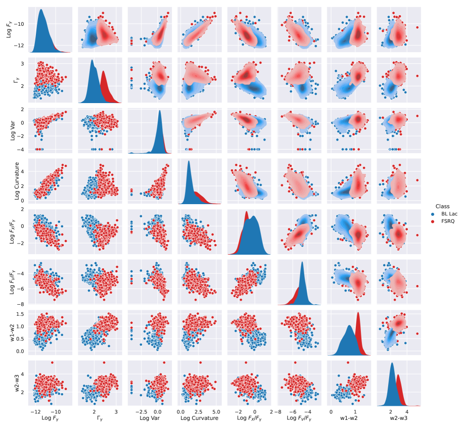
Figure 1: Full pair plots of all the eight parameters described in Section 3. Blue and Red colors correspond to the BL Lacs (671) and FSRQs respectively. The diagonal plots are smoothed histogram distributions of parameters for each class of sources. Off-diagonal plots in the upper and lower regions are the Kernel Density Estimate (KDE) and scatter plots for different parameters respectively.

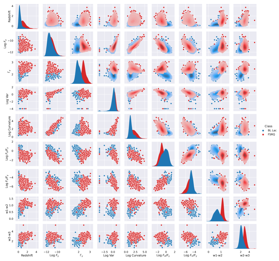
Figure 2: Full pair plots of all the nine parameters described in Set B. Blue and Red colors correspond to the BL Lacs (479) and FSRQs (407) respectively. The diagonal plots are smoothed histogram distributions of parameters for each class. The plots in the upper and lower diagonal are the Kernel Density Estimate (KDE) and scatter plots for different parameters respectively.

4 Extreme Gradient Boosting (XGBoost)

In this work, we investigate the potential of eXtreme Gradient Boosting (XGBoost) algorithm for classification of blazar candidates. It is a supervised machine learning algorithm which has been developed on the basis of Gradient Boosting Decision Tree (GBDT), also known as gradient boosting machine or gradient boosted regression tree (Friedman, 2001; Chen & Guestrin, 2016). XGBoost classifier, a scalable machine learning system, has appeared more recently and is able to provide state-of-the-art results with stability on a wide range of problems in the fields of machine learning and data mining challenges. In recent times, it has been used in astronomy for different purposes including classification of gamma-ray sources detected by the Fermi-LAT (Li et al., 2019; Li et al., 2021; Ivanov et al., 2021; Agarwal, 2023; Sahakyan et al., 2023). The scalability of XGBoost is attributed to several innovative algorithmic optimizations including a novel tree learning algorithm to handle the sparse data and a theoretically justified weighted quantile sketch procedure for handling instance weights in approximate tree learning (Chen & Guestrin, 2016).

Similar to the GBDT, the XGBoost algorithm applies boosting method and builds strong classifiers by means of learning multiple weak classifiers sequentially. However the XGBoost excels in performance and efficiency and also differs from the GBDT in the calculation of residuals. Both the first and second derivatives of the loss function are used for calculating the residuals in the XGBoost whereas only first derivative is used in the case of GBDT. The XGBoost model typically consists of a certain number of trees. The first tree is constructed after applying a cost function which tests all features and chooses the best features and conditions from data. Specifically, the feature with the highest gain is chosen as the root node, and its corresponding condition is decided during the first epoch of testing. Subsequently, features are chosen and added to the tree as internal nodes one by one recursively until the tree grows to the specified depth or the maximum depth. The ends of branches are called leaves and they hold the results of the tree. The results in leaf nodes decide degree of an unknown source to belong to a particular class. Similarly, the $(i+1)^{th}$ tree is built in the same way as the first tree, except that the aim of this tree is to fit the residuals i.e. the measurement of the difference between the predicted and the original target of the previous model consisting of $i$-trees rather than the original target. The residuals are fitted with a certain learning rate which is related to the step size of the fitting. Finally, the process of building the XGBoost classifier stops when a specific number of trees or number of estimators has been built. In the present work, we have used XGBoost python package provided by scikit-learn as an open source (Pedregosa et al., 2011). Application of XGBoost machine learning algorithm for identifying the exact nature of BCUs is described below.

4.1 Data Balancing with SMOTE

The Synthetic Minority Over-sampling Technique (SMOTE) is used in astronomy to deal with the imbalanced data sets (Bethapudi & Desai, 2018; Sutrisno et al., 2019; Carruba et al., 2023). It has also been used for classification of gamma-ray sources (Kaur et al., 2019; Kaur et al., 2021, 2023). In the present work, the number of BL Lacs is more than that of the FSRQs in both data Set A & B (Section 3). Thus, the two blazar subclasses are not equally represented in the data sets for training the XGBoost algorithm. Such imbalance in the data leads to the selection effects in the ensemble based algorithms which may be biased against the under represented classes (Last et al., 2017). In order to balance the representation of BL Lacs and FSRQs in the data Set A & B, we employ Synthetic Minority Over-sampling Technique (SMOTE) for generating additional synthetic members of the under represented blazar subclass (i.e. FSRQ) using k-nearest neighbor approach (Chawla et al., 2002). As a result of the SMOTE expansion, the data Set A & B now contain original BL Lacs and FSRQs as well as new synthetic FSRQs generated with the same distribution in parameter-space as the real FSRQs. Thus, the training data samples in Set A and Set B are balanced with a total of 671 FSRQs/BL Lacs and 479 FSRQs/BL Lacs respectively. A comparison of the Pre-SMOTE and Post-SMOTE smoothed distributions of each parameter for FSRQs in Set A and Set B is presented in Figures 3 and 4 respectively. It is observed that changes in distributions of the parameters are minimal and the artificially generated FSRQs mimic the original FSRQs in both the data sets. These balanced data sets are used for training the XGBoost algorithm to classify the BCUs among FSRQs and BL Lacs.

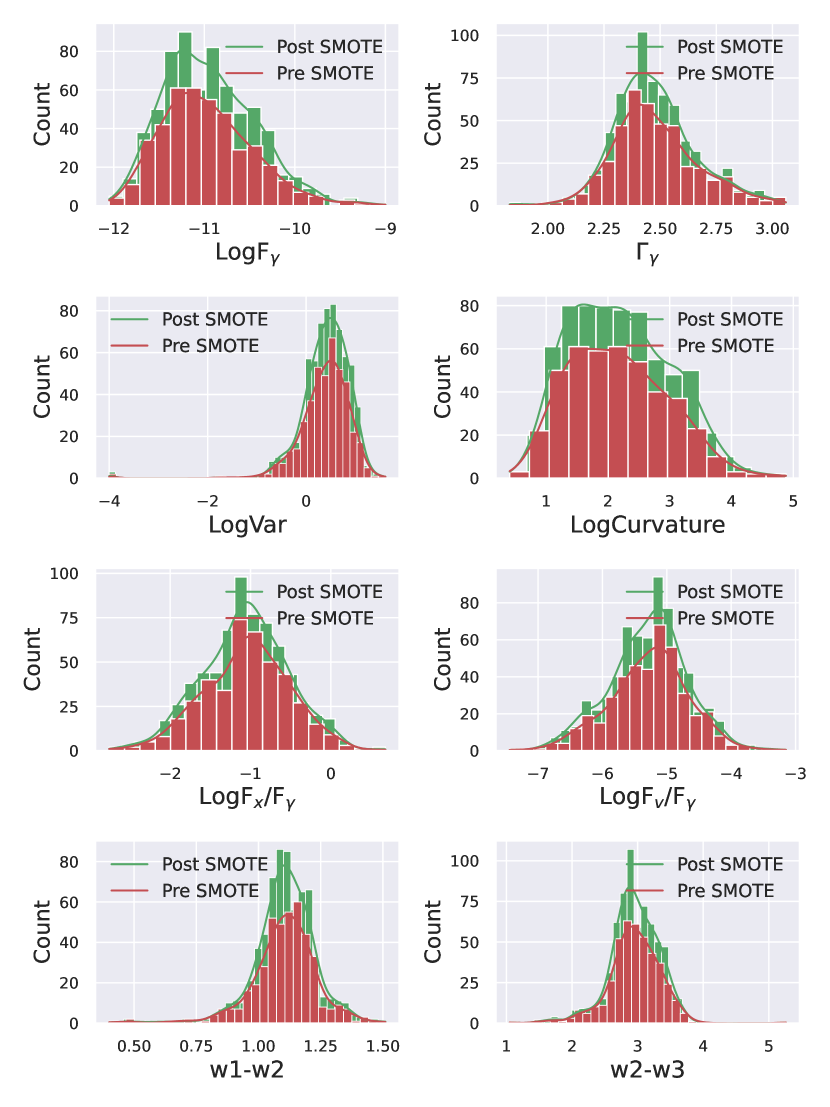
Figure 3: Smoothed distributions of the eight parameters of the FSRQs before and after employing SMOTE for balancing the data in Set A. The two distributions for all the parameters are almost identical and hence the synthetically generated FSRQs follow the distributions of original FSRQs.

Figure 4: Smoothed distributions of the nine parameters of the FSRQs before and after the application of SMOTE for data balancing in in Set B. Here also, the two distributions are identical.

4.2 Training and Validation

We use the blazar data samples described in Set A and Set B, with eight and nine input parameters respectively, for training and validation of the XGBoost algorithm in the present work. We define two XGBoost models namely XGB and XGBz corresponding to the Set A and Set B respectively. The main difference between the two models is the number of input parameters to each model. We randomly split each data set into training and validation data sets in 80:20 ratio so that the two data samples are balanced. Thus, out of 1342 blazars (original$+$SMOTE) in Set A, 1073 blazars are randomly selected for training and remaining 269 blazars for validation of the XGB model. Similarly in case of Set B, 766 and 192 blazars amongst the total 958 blazar (original$+$SMOTE) samples are reserved for training and validation of the XGBz model. Application of trained model on the unassociated sources in the validation data set returns a set of probability values referred to as FSRQness for each source. The FSRQness value indicates probability of a source likely to be an FSRQ. For the predictions, the evaluation regards the instances with FSRQness value greater than 0.5 as FSRQs and others as BL Lacs. We optimize the model parameters by minimizing the binary classification error rates on the validation data sets for both the models. The classification error rate is calculated as

$$\rm Error~{}rate=\frac{\rm number~{}of~{}wrong~{}predictions}{\rm total~{}number~{}of~{}predictions}$$ (1)

We monitor the performance of a model on each training epoch by evaluating the classification error rate on both training as well as validation data sets. As the training progresses on different epochs, classification error rate continuously decreases for the training data set as the model learning improves. However, for validation data the error rate first decreases as the model gets trained and after certain epochs the error rate remain same and then it starts increasing as the model overfits the training data. We stop the training when the error rate does not change since further training will have negative impact on the predictive capabilities of the model on unknown data. The final XGB model consists of 380 trees (total number of estimators), each having depth of 3 (maximum depth) and a learning rate of 0.1. Whereas, the optimized XGBz model has 535 trees, each with depth 2 and a learning rate of 0.1. All other hyper-parameters of the model are set to their default values.

4.3 Model Performance Evaluation

In machine learning based studies, evaluation metrics are generally used to quantify the the performance of an algorithm or classifier. We apply the trained models XGB and XGBz on validation data of Set A and Set B respectively to calculate three standard metrics corresponding to the accuracy, precision and recall to determine model performance. Accuracy is defined as the fraction of total number of correct predictions among the total number of predictions. Precision is the ratio of true positive predictions to all the positively predicted examples. Recall is the ratio of true positive predictions to all the true positive examples. Qualitatively, Recall is a measure of sensitivity of a model to a particular class and it represents the capability of a model to find all the relevant cases within a data set whereas Precision is the ability of a classifier to identify only the relevant data points. Precision and Recall are defined for each class, whereas the Accuracy is defined for whole data set. A summary of the performance evaluation of the two models using Accuracy, Precision and Recall metrics is provided in Table 1. It is observed that the XGB and XGBz models predict class of the unassociated sources with an accuracy of 96$\%$ and 92$\%$ respectively. The confusion matrices for both the models are also shown in Figure 5. The confusion matrix is a specific table layout that summarizes the prediction results of a classification model in machine learning. It describes the data in a matrix form according to two criteria namely the real category and the prediction judgement made by the classification model.

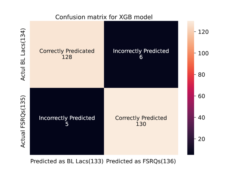
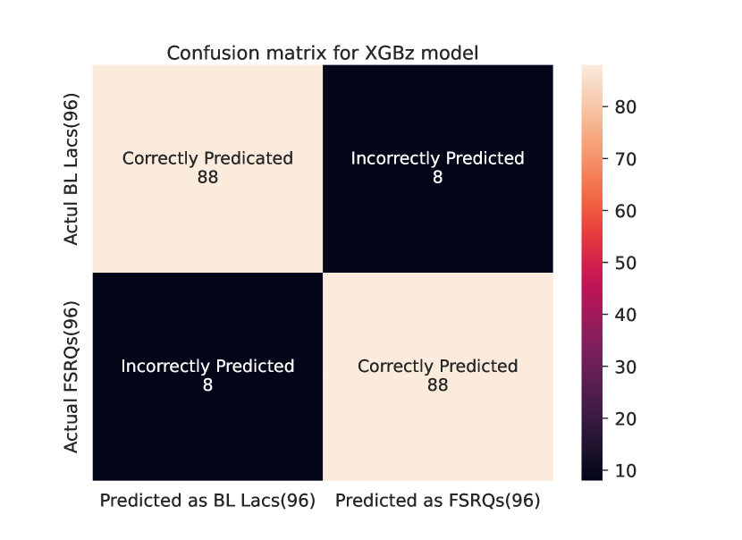
Figure 5: Confusion matrices for the XGBoost classifiers XGB and XGBz on 269 and 192 known sources respectively.

5 Results and Discussion

Machine learning algorithms are used as probabilistic classifiers of unassociated source. In this work, we apply XGBoost method, a supervised machine learning algorithm, to identify the BL Lacs and FSRQ subclasses among the sample of selected blazars of uncertian type. Main results of this study are discussed below:

5.1 Classification of BCUs

We employ the trained models XGB and XGBz (subsection 4.2) on the sample of BCUs in Set A and Set B respectively. During validation of the algorithm, we have classified sources to be likely FSRQ if FSRQness $>$ 0.5 and likely BL Lacs if FSRQness $<$ 0.5. But we adopt a more strict and conservative approach while classifying the BCUs. We define sources to be highly likely FSRQ if FSRQness $>$ 0.99, highly likely BL Lacs if FSRQness $<$ 0.01 and remaining as ambiguous-type blazars. The associated class and corresponding FSRQness value for each source classified in the present work using the XGB and XGBz models along with the corresponding results reported by K23 are summarized in Tables 2, and 3. Results obtained in the present work with data Set A and B are discussed below:

5.1.1 Set A

There are 112 BCUs in Set A for classification. Application of XGB model on this data sample results in the identification of 6 sources as highly likely FSRQ, 62 sources as highly likely BL Lacs and remaining 44 sources as ambiguous-type blazars. These numbers indicate a significant improvement in the earlier classification of the same sample using the neural networks reported by K23 (Kaur et al., 2023) wherein 4 sources are identified as highly likely FSRQs, 50 sources as highly likely BL Lacs and remaining 58 sources as ambiguous-type blazars. A comparison of the performance of XGB model with that of the neural networks (K23) in terms of the number of sources is shown in Figure 6. The distributions of FSRQness values of sources classified as BL Lacs and FSRQs using XGB model and neural networks (K23) are shown in Figure 7. It is observed that the mean of FSRQness values obtained from XGB model for classified BL Lacs (FSRQs) is closer to 0 (1) than FSRQness values of classified BL Lacs (FSRQs) reported by K23. With XGB model, the mean of FSRQness values of classified BL Lacs (FSRQs) is 0.0029 (0.9952), whereas with the neural network methods the mean of FSRQness values of classified BL Lacs (FSRQs) is 0.0071 (0.9923). This indicates that XGBoost based XGB model classifies the sources with more confidence/decisiveness by associating relatively higher probabilities (for belonging to a particular class) to the sources compared to neural networks based algorithm reported by K23. Therefore, the results obtained in the present work suggest that the XGBoost algorithm classifies the sample of 112 BCUs better than the neural network based methods.

5.1.2 Set B

Out of 112 BCUs in Set A, redshifts of only 37 sources are available for classification in Set B. Application of XGBz model on the sample of 37 BCUs classifies 4 sources as highly likely FSRQs, 27 sources as highly likely BL Lacs and 6 sources as ambiguous-type blazars. This is compared with the output of XGB model and results reported by K23 without using $z$ information in Figure 8. The XGB model (K23) classification of these 37 BCUs results into 4(3) as highly likely FSRQs, 24(22) highly likely BL Lacs and 9(12) as ambigous-type blazars. This implies that the XGBz model provides a better classification than the XGB model and the neural network approach. The list of sources that change the classification in XGBz model compared to XGB model are tabulated in Table 4. The 6 ambiguous XGB sources are reclassified as FSRQs/BL Lacs by the XGBz model with 8.73$\%$ change in mean FSRQness. However, 3 classified XGB sources are identified as ambiguous by XGBz model with 1.4$\%$ change in mean FSRQness. Effectively, 3 additional sources are classified by the XGBz as compared to XGB model. But the data sample of 37 BCUs is not significant enough to establish the robust impact of redhsift in the classification of these sources. Figure 9 shows the distributions of FSRQness values of sources classified as BL Lacs and FSRQs using XGB and XGBz models. This suggests that the mean of FSRQness values obtained from XGBz model for classified BL Lacs (FSRQs) is slightly close to 0 (1) as compared to FSRQness values of classified BL Lacs (FSRQs) obtained from XGB model. Using XGBz model, the obtained mean of FSRQness values of classified BL Lacs (FSRQs) is 0.0014 (0.9968), whereas with XGB model the mean of FSRQness values of classified BL Lacs (FSRQs) is 0.002 (0.9950). Therefore, use of redshift as an additional parameter in XGBz model has an impact on the classification, but more number of BCUs with redshift information is required to comment on its significance and robustness.

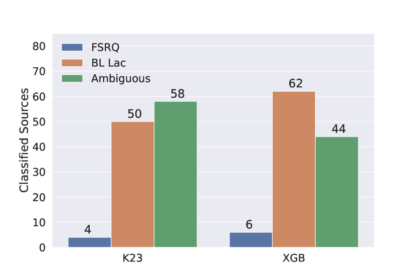
Figure 6: Comparison of the classification of 112 BCUs using XGB model with the results reported by K23 (Kaur et al., 2023).

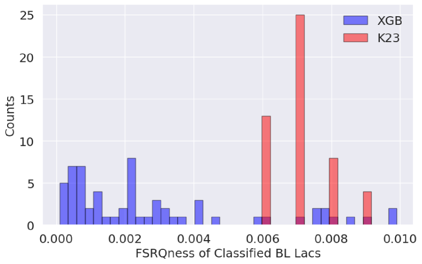
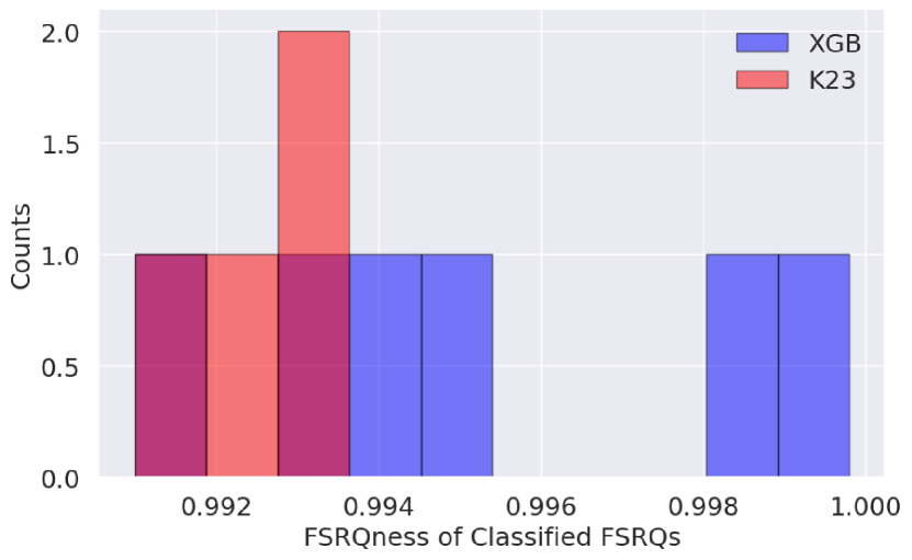
Figure 7: Distribution of FSRQness values of classified BL Lacs and FSRQs using XGB model and results reported by K23 (Kaur et al., 2023).

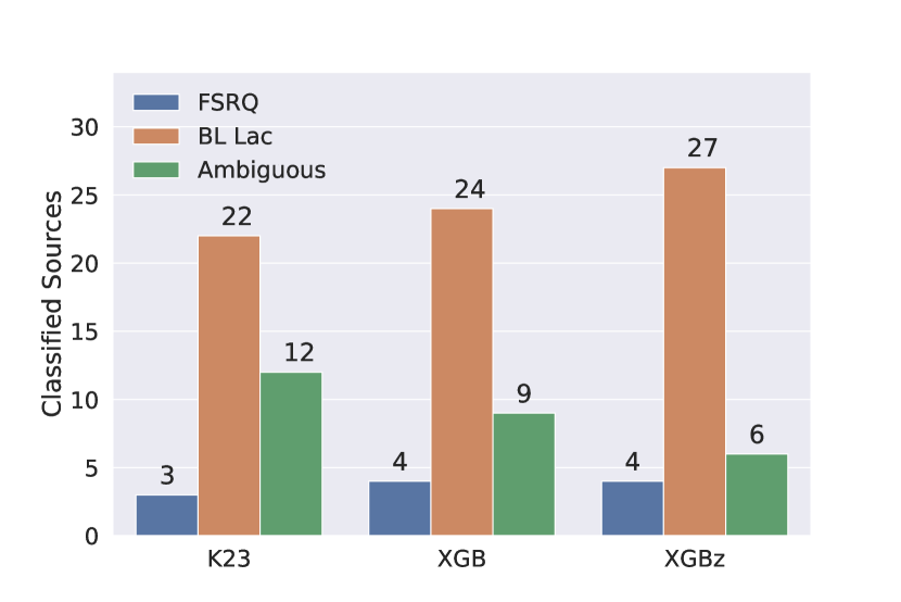
Figure 8: Comparison of the classification of 37 BCUs with known redshift using XGBz model with the XGB model and results reported by K23 (Kaur et al., 2023).

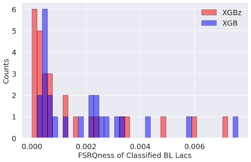
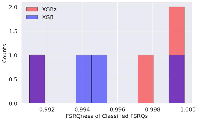
Figure 9: Distribution of FSRQness values of classified BL Lacs and FSRQs using XGB and XGBz model.

5.2 Feature Importance

In machine learning algorithms, feature importance is estimated to rank the importance of each input feature/parameter. It basically represents the relative weight of the variables and indicates how useful or valuable each feature is in the construction of the boosted decision trees within the model. The more a feature is used to make key decisions with decision trees, its relative importance will be higher. This is explicitly calculated for each feature in the in the data set, allowing attributes to be ranked in comparison to each other. Importance is calculated for a single decision tree by the amount each attribute split point improves the performance measure, weighted by the number of observations the node is responsible for. The feature importances are then averaged across all the decision trees within the model (Hastie et al., 2016). We have calculated the feature importances of each attribute in the data Sets A and B described in Section 3 for the models XGB and XGBz respectively. The same are plotted in Figure 10 for the two models used in this work. It is observed that the gamma-ray photon index parameter ($\Gamma_{\gamma}$; PL_Index) is the dominant feature in deciding the subclass of blazars for both the models. This is in agreement with the distribution plots in Figure 1 wherein $\Gamma_{\gamma}$-distributions for BL Lacs and FSRQs are nicely separated. The WISE infra-red color indices (w1-w2 and w2-w3) are the second and third most dominant features in the classification. Therefore IR data play an important role in classifying the BCUs. Classification of blazars, based on the observational features, offers unique opportunity to identify key characteristics and probe the physical processes involved in their broadband emissions. For example, IR measurements involve contributions from the jet and molecular torus for FSRQs whereas gamma-ray observations only probe the non-thermal emission of the beamed jet. FSRQs usually have a steep gamma-ray spectrum in the GeV-TeV domain while BL Lacs (mainly HBLs) show hard spectrum (Prandini & Ghisellini, 2022).

As discussed earlier, the main difference between XGB and XGBz models is the use of redshift ($z$) information as an additional feature. From Figure 10, it is evident that $z$ is the fourth most dominant parameter in deciding the class of BCUs using the XGBz model. The XGBz model has performed better than the XGB model during the classification of a sample of 37 BCUs mainly because of the use of redshift information. Even though redshift has played a role in classification, but it is not the dominant feature. We need a large sample of BCUs with known redshift to establish the explicit role of redshift in the identification of blazar subclasses more robustly. Also distinct and well separated distributions of redshift for BL Lacs and FSRQs in Figure 2 reflect a bias in observation of two types of blazars. Since BL Lacs have weak or no spectral lines, their redshift measurement is a challenge as compared to FSRQs.

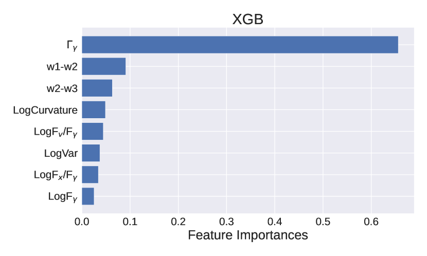
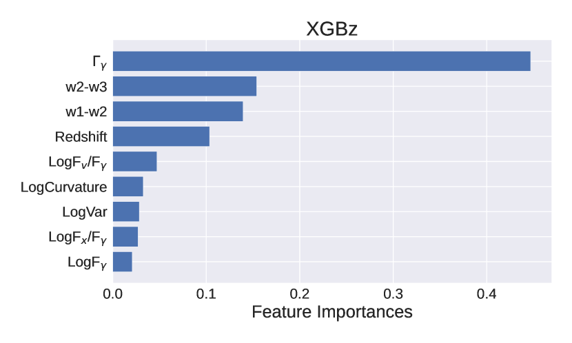
Figure 10: Relative importance of different input parameters or variables in the XGB and XGBz models for classification of blazar candidates of uncertain type.

6 Summary

The present work underscores the potential of XGBoost algorithm for the classification of blazar candidates of uncertain type and compares its performance with the neural network classifiers. Results obtained in this work indicate a significant improvement in the classification of 112 candidates as compared to the neural networks based approach of K23 Kaur et al. (2023). The main findings of this study are summarized below:

• The gradient boosting classifier based on the XGBoost implementations is found to be a data efficient alternative to the neural network based classifiers. Also, it is relatively straightforward to retrieve the importance scores for each attribute after the decision trees are constructed in the gradient boosting implementations. The XGBoost algorithm is able to better classify the sources with more robustness/decisiveness than neural networks. Efficacy and accuracy of the XGBoost classifier may outperform the other machine learning based classifiers in the identification of the exact nature of blazar candidates of uncertain type.

• Out of 112 blazar candidates of uncertain type, the XGBoost classifier is able to identify 6 sources as FSRQ and 62 objects as BL Lacs with very high accuracy using only multi-wavelength information. The mean of FSRQness values of classified BL Lacs (FSRQs) is 0.0029 (0.9952), whereas with the neural network methods the mean of FSRQness values of classified BL Lacs (FSRQs) is 0.0071 (0.9923).

• Among the eight observational features used for classification, gamma-ray spectral index and IR color indices play dominant role in identifying the blazar subclasses among the blazar candidates of uncertain type.

• Use of redshift as an additional feature leads to the identification of 4 sources as FSRQs and 27 sources as BL Lacs in the sample of 37 BCUs. Without using redshift information, only 24 sources are classified as BL Lacs in the same sample of 37 BCUs whereas the identification of FSRQs is unchanged.

• Redshift of the blazars is found to play a role in the classification of the blazar candidates of uncertain type. It is supported by the observational fact that BL Lac type blazars are located at smaller redshift and FSRQs are mostly located at high redshifts. But a more rigorous investigation of a large sample of BCUs with known redshift is needed to establish the importance of redshift in blazar classification since there is a bias in the redshift measurements of FSRQs as compared to BL Lacs.

Over the last two decades, rapid development in field of ground-based gamma-ray astronomy, using state-of-the-art imaging atmospheric Cherenkov telescopes, has provided detection of more than 80 blazars in the GeV-TeV energy range. Among these blazars, about 70 have a measured/known redshifts. This emerging population of TeV blazars offers a new perspective to be investigated in future as a large fraction of BCUs detected by the Fermi-LAT still remains unassociated. The information derived from the ground-based observations such as photon spectral index in the TeV energy range along with the redshift will be more effective in the classification of the blazar candidates of uncertain type using the potential of XGBoost machine learning algorithm explored in the present work.

Data Availability

Data used in this work is derived from the literature and can be shared on reasonable request.

References

- Abdo et al. (2010) Abdo A. A., et al., 2010, ApJ, 716, 30
- Abdollahi et al. (2020) Abdollahi S., et al., 2020, ApJS, 247, 33
- Abdollahi et al. (2022) Abdollahi S., et al., 2022, ApJS, 260, 53
- Ackermann et al. (2012) Ackermann M., et al., 2012, ApJ, 753, 83
- Ackermann et al. (2015) Ackermann M., et al., 2015, ApJ, 810, 14
- Ackermann et al. (2016) Ackermann M., et al., 2016, ApJS, 222, 5
- Agarwal (2023) Agarwal A., 2023, ApJ, 946, 109
- Aharonian (2002) Aharonian F. A., 2002, MNRAS, 332, 215
- Ajello et al. (2017) Ajello M., et al., 2017, ApJS, 232, 18
- Ajello et al. (2020) Ajello M., et al., 2020, ApJ, 892, 105
- Ajello et al. (2021) Ajello M., et al., 2021, ApJS, 256, 12
- Ajello et al. (2022) Ajello M., et al., 2022, ApJS, 263, 24
- Atwood et al. (2009) Atwood W. B., et al., 2009, ApJ, 697, 1071
- Balakrishnan et al. (2021) Balakrishnan V., Champion D., Barr E., Kramer M., Sengar R., Bailes M., 2021, MNRAS, 505, 1180
- Baron (2019) Baron D., 2019, arXiv e-prints, p. arXiv:1904.07248
- Bethapudi & Desai (2018) Bethapudi S., Desai S., 2018, Astronomy and Computing, 23, 15
- Blandford & Payne (1982) Blandford R. D., Payne D. G., 1982, MNRAS, 199, 883
- Blandford et al. (2019) Blandford R., Meier D., Readhead A., 2019, ARA&A, 57, 467
- Böttcher et al. (2013) Böttcher M., Reimer A., Sweeney K., Prakash A., 2013, ApJ, 768, 54
- Carruba et al. (2023) Carruba V., Aljbaae S., Caritá G., Lourenço M. V. F., Martins B. S., Alves A. A., 2023, Frontiers in Astronomy and Space Sciences, 10, 1196223
- Chawla et al. (2002) Chawla N. V., Bowyer K. W., Hall L. O., Kegelmeyer W. P., 2002, Journal of artificial intelligence research, 16, 321
- Chen & Guestrin (2016) Chen T., Guestrin C., 2016, in Proceedings of the 22nd acm sigkdd international conference on knowledge discovery and data mining. pp 785–794
- Chiaro et al. (2016) Chiaro G., Salvetti D., La Mura G., Giroletti M., Thompson D. J., Bastieri D., 2016, MNRAS, 462, 3180
- Chiaro et al. (2021) Chiaro G., Kovacevic M., La Mura G., 2021, Journal of High Energy Astrophysics, 29, 40
- Costamante et al. (2001) Costamante L., et al., 2001, A&A, 371, 512
- Dermer (2015) Dermer C. D., 2015, Mem. Soc. Astron. Italiana, 86, 13
- Doert & Errando (2013) Doert M., Errando M., 2013, in International Cosmic Ray Conference. p. 3032 (arXiv:1306.6529), doi:10.48550/arXiv.1306.6529
- Friedman (2001) Friedman J. H., 2001, Annals of statistics, pp 1189–1232
- Ghisellini et al. (2009) Ghisellini G., Maraschi L., Tavecchio F., 2009, MNRAS, 396, L105
- Ghisellini et al. (2011) Ghisellini G., Tavecchio F., Foschini L., Ghirlanda G., 2011, MNRAS, 414, 2674
- Ghosal et al. (2022) Ghosal B., et al., 2022, MNRAS, 517, 5473
- Giommi et al. (2012) Giommi P., Padovani P., Polenta G., Turriziani S., D’Elia V., Piranomonte S., 2012, MNRAS, 420, 2899
- Giommi et al. (2021) Giommi P., et al., 2021, MNRAS, 507, 5690
- Hassan et al. (2013) Hassan T., Mirabal N., Contreras J. L., Oya I., 2013, MNRAS, 428, 220
- Hastie et al. (2016) Hastie T., Tibshirani R., Friedman J., 2016, The Elements of Statistical Learning: Data Mining, Inference, and Prediction
- Ivanov et al. (2021) Ivanov S., Tsizh M., Ullmann D., Panos B., Voloshynovskiy S., 2021, Astronomy and Computing, 36, 100473
- Kang et al. (2019) Kang S.-J., Li E., Ou W., Zhu K., Fan J.-H., Wu Q., Yin Y., 2019, ApJ, 887, 134
- Kaur et al. (2019) Kaur A., Falcone A. D., Stroh M. D., Kennea J. A., Ferrara E. C., 2019, ApJ, 887, 18
- Kaur et al. (2021) Kaur A., Falcone A. D., Stroh M. C., 2021, ApJ, 908, 177
- Kaur et al. (2023) Kaur A., Kerby S., Falcone A. D., 2023, ApJ, 943, 167
- Kerby et al. (2021) Kerby S., et al., 2021, ApJ, 923, 75
- Kovačević et al. (2019) Kovačević M., Chiaro G., Cutini S., Tosti G., 2019, MNRAS, 490, 4770
- Kovačević et al. (2020) Kovačević M., Chiaro G., Cutini S., Tosti G., 2020, MNRAS, 493, 1926
- Last et al. (2017) Last F., Douzas G., Bacao F., 2017, arXiv e-prints, p. arXiv:1711.00837
- Lee et al. (2012) Lee K. J., Guillemot L., Yue Y. L., Kramer M., Champion D. J., 2012, MNRAS, 424, 2832
- Li et al. (2019) Li C., Zhang W. H., Lin J. M., 2019, Acta Astronomica Sinica, 60, 16
- Li et al. (2021) Li C., et al., 2021, MNRAS, 506, 1651
- Lott et al. (2020) Lott B., Gasparrini D., Ciprini S., 2020, arXiv e-prints, p. arXiv:2010.08406
- Marchesini et al. (2019) Marchesini E. J., et al., 2019, Ap&SS, 364, 5
- Marscher & Gear (1985) Marscher A. P., Gear W. K., 1985, ApJ, 298, 114
- Massaro et al. (2013) Massaro F., D’Abrusco R., Paggi A., Masetti N., Giroletti M., Tosti G., Smith H. A., Funk S., 2013, ApJS, 209, 10
- Mirabal et al. (2012) Mirabal N., Frías-Martinez V., Hassan T., Frías-Martinez E., 2012, MNRAS, 424, L64
- Netzer (2015) Netzer H., 2015, ARA&A, 53, 365
- Nun et al. (2014) Nun I., Pichara K., Protopapas P., Kim D.-W., 2014, ApJ, 793, 23
- Pedregosa et al. (2011) Pedregosa F., et al., 2011, Journal of Machine Learning Research, 12, 2825
- Potter & Cotter (2013) Potter W. J., Cotter G., 2013, MNRAS, 436, 304
- Prandini & Ghisellini (2022) Prandini E., Ghisellini G., 2022, Galaxies, 10, 35
- Sahakyan et al. (2023) Sahakyan N., Vardanyan V., Khachatryan M., 2023, MNRAS, 519, 3000
- Sahu et al. (2021) Sahu S., López Fortín C. E., Valadez Polanco I. A., Rajpoot S., 2021, ApJ, 914, 120
- Salvetti et al. (2017) Salvetti D., Chiaro G., La Mura G., Thompson D. J., 2017, MNRAS, 470, 1291
- Singh & Meintjes (2020) Singh K. K., Meintjes P. J., 2020, Astronomische Nachrichten, 341, 713
- Singh et al. (2019a) Singh K. K., Dhar V. K., Meintjes P. J., 2019a, Experimental Astronomy, 48, 297
- Singh et al. (2019b) Singh K. K., Meintjes P. J., Ramamonjisoa F. A., Tolamatti A., 2019b, New Astron., 73, 101278
- Singh et al. (2019c) Singh K. K., Bisschoff B., van Soelen B., Tolamatti A., Marais J. P., Meintjes P. J., 2019c, MNRAS, 489, 5076
- Singh et al. (2022a) Singh K. K., Tolamatti A., Godiyal S., Pathania A., Yadav K. K., 2022a, Universe, 8, 539
- Singh et al. (2022b) Singh K. K., Dhar V. K., Meintjes P. J., 2022b, New Astron., 91, 101701
- Singh et al. (2022c) Singh K. P., Kushwaha P., Sinha A., Pal M., Agarwal A., Dewangan G. C., 2022c, MNRAS, 509, 2696
- Sol & Zech (2022) Sol H., Zech A., 2022, Galaxies, 10, 105
- Stocke et al. (1991) Stocke J. T., Morris S. L., Gioia I. M., Maccacaro T., Schild R., Wolter A., Fleming T. A., Henry J. P., 1991, ApJS, 76, 813
- Sutrisno et al. (2019) Sutrisno R., Vilalta R., Renshaw A., 2019, in Teuben P. J., Pound M. W., Thomas B. A., Warner E. M., eds, Astronomical Society of the Pacific Conference Series Vol. 523, Astronomical Data Analysis Software and Systems XXVII. p. 115
- Tolamatti et al. (2022) Tolamatti A., et al., 2022, Astroparticle Physics, 139, 102687
- Urry & Padovani (1995) Urry C. M., Padovani P., 1995, PASP, 107, 803
- Yamada et al. (2020) Yamada Y., Uemura M., Itoh R., Fukazawa Y., Ohno M., Imazato F., 2020, PASJ, 72, 42
- von Kienlin et al. (2020) von Kienlin A., et al., 2020, ApJ, 893, 46