11email: stefano.bellotti@irap.omp.eu 22institutetext: Science Division, Directorate of Science, European Space Research and Technology Centre (ESA/ESTEC), Keplerlaan 1, 2201 AZ, Noordwijk, The Netherlands 33institutetext: Leiden Observatory, Leiden University, PO Box 9513, 2300 RA Leiden, The Netherlands 44institutetext: Department of Physics, College of Science, United Arab Emirates University, P.O. Box No. 15551, Al Ain, UAE
44email: rim.fares@uaeu.ac.ae 55institutetext: Laboratoire Univers et Particules de Montpellier, Université de Montpellier, CNRS, F-34095, Montpellier, France 66institutetext: Observatoire Astronomique de l’Université de Genéve, Chemin Pegasi 51b, 1290 Versoix, Switzerland
The space weather around the exoplanet GJ 436b
Abstract
Context. The space environment in which planets are embedded depends mainly on the host star and impacts the evolution of the planetary atmosphere. The quiet M dwarf GJ 436 hosts a close-in hot Neptune which is known to feature a comet-like tail of hydrogen atoms escaped from its atmosphere due to energetic stellar irradiation. Understanding such star-planet interactions is essential to shed more light on planet formation and evolution theories, in particular the scarcity of Neptune-size planets below 3 d orbital period, also known as “Neptune desert”.
Aims. We aimed at characterising the stellar environment around GJ 436, which requires an accurate knowledge of the stellar magnetic field. The latter is studied efficiently with spectropolarimetry, since it is possible to recover the geometry of the large-scale magnetic field by applying tomographic inversion on time series of circularly polarised spectra.
Methods. We used spectropolarimetric data collected in the optical domain with Narval in 2016 to compute the longitudinal magnetic field, examine its periodic content via Lomb-Scargle periodogram and Gaussian Process Regression analysis, and finally reconstruct the large-scale field configuration by means of Zeeman-Doppler Imaging.
Results. We found an average longitudinal field of 12 G and a stellar rotation period of 46.6 d using a Gaussian Process model and 40.1 d using Zeeman-Doppler Imaging, both consistent with the literature. The Lomb-Scargle analysis did not reveal any significant periodicity. The reconstructed large-scale magnetic field is predominantly poloidal, dipolar and axisymmetric, with a mean strength of 16 G. This is in agreement with magnetic topologies seen for other stars of similar spectral type and rotation rate.
Key Words.:
Stars: magnetic field – Stars: individual: GJ 436 – Stars: activity – Techniques: polarimetric1 Introduction
The stellar environment in which exoplanets are immersed has a significant impact on their atmospheres. Energetic phenomena associated with intense magnetic activity such as frequent flares can alter the chemical properties of the planetary atmosphere (Segura et al., 2010; Günther et al., 2020; Konings et al., 2022; Louca et al., 2023), with hazardous consequences for habitability (e.g., Tilley et al., 2019). In particular for planets orbiting closer ( au) to the host star, energetic stellar irradiation (X-rays and extreme ultra-violet) heats and expands the upper regions of the atmosphere, resulting in hydrodynamic escape (e.g., Lammer et al., 2003; Vidal-Madjar et al., 2003; Owen & Jackson, 2012). In addition to the radiation from the host star, stellar particles from magnetised wind and coronal mass ejections also impact planetary atmospheres, e.g., by confining and stripping them away (Carolan et al., 2021; Hazra et al., 2022). Evaporation of planetary atmospheres is accentuated in the early stages of a planetary system (Ribas et al., 2005; Allan & Vidotto, 2019; Ketzer & Poppenhaeger, 2023), and is one of the mechanisms proposed to explain the “Neptune desert”, i.e. the paucity of planets with masses between 0.01 and 1 MJup in short-distance orbits (e.g., Lecavelier Des Etangs, 2007; Penz et al., 2008; Davis & Wheatley, 2009; Ehrenreich & Désert, 2011; Beaugé & Nesvorný, 2013; Lundkvist et al., 2016; Mazeh et al., 2016). Likewise, photoevaporation can make a mini-Neptune lose a significant amount of hydrogen and helium, morphing it into a potentially habitable super-Earth (Luger et al., 2015).
| Date | UT | HJD | S/N | Bl | |||
|---|---|---|---|---|---|---|---|
| [hh:mm:ss] | [-2457464.4967] | [s] | [] | [G] | |||
| Mar 16 | 23:49:19 | 0.00 | 0.00 | 4x700 | 201 | 5.7 | 12.37.0 |
| Mar 18 | 00:36:58 | 1.03 | 0.03 | 4x700 | 202 | 5.6 | 8.06.8 |
| Mar 20 | 23:25:14 | 3.98 | 0.10 | 4x700 | 271 | 4.0 | 4.05.0 |
| Apr 18 | 21:33:54 | 32.91 | 0.82 | 4x700 | 231 | 4.6 | 0.96.0 |
| May 02 | 23:10:51 | 46.97 | 1.17 | 4x700 | 265 | 4.0 | 14.85.0 |
| May 03 | 23:32:45 | 47.99 | 1.20 | 4x700 | 220 | 5.7 | 11.56.6 |
| May 04 | 21:30:12 | 48.90 | 1.22 | 4x700 | 229 | 4.8 | 14.86.0 |
| May 11 | 20:34:43 | 55.86 | 1.39 | 4x700 | 190 | 6.5 | 12.37.4 |
| May 16 | 20:45:50 | 60.87 | 1.52 | 4x700 | 270 | 3.9 | 23.15.0 |
| May 17 | 20:46:53 | 61.87 | 1.54 | 4x700 | 188 | 5.8 | 19.67.4 |
| May 20 | 21:13:31 | 64.89 | 1.62 | 4x700 | 210 | 5.9 | 21.96.7 |
| May 23 | 20:54:26 | 67.88 | 1.69 | 4x700 | 228 | 5.1 | 17.46.1 |
| Jun 02 | 20:58:28 | 77.88 | 1.94 | 4x700 | 214 | 5.2 | 9.16.5 |
| Jun 04 | 21:10:44 | 79.89 | 1.99 | 4x700 | 204 | 5.6 | 2.76.8 |
| Jun 07 | 20:59:19 | 82.88 | 2.07 | 4x700 | 265 | 3.9 | 11.35.1 |
| Jun 08 | 21:04:34 | 83.88 | 2.09 | 4x700 | 278 | 3.8 | 6.54.7 |
Characterising the space weather for a specific system and modelling the interaction between the magnetised stellar wind and a close-in planet requires robust knowledge of the stellar magnetic field (Vidotto et al., 2014a, b). Our assumptions on its topology and strength indeed impact the extent of the planetary magnetosphere (Villarreal D’Angelo et al., 2018; Carolan et al., 2021) and predictions of transits duration (Llama et al., 2013). Stellar magnetic fields are most effectively studied using spectropolarimetry, with which we can analyse the Zeeman effect, i.e. the splitting of spectral lines in distinct components characterised by specific polarisation properties (Zeeman, 1897). From time series of polarised spectra we can map the large-scale magnetic field by means of Zeeman-Doppler Imaging (ZDI; Semel 1989; Donati & Brown 1997) and obtain a global picture of the magnetic environment. Zeeman-Doppler Imaging has been applied extensively in spectropolarimetric studies, and revealed a variety of field geometries for low-mass stars (e.g., Petit et al., 2005; Donati et al., 2008; Morin et al., 2008, 2010; Fares et al., 2013, 2017).
GJ 436 is a quiet M2.5 dwarf and hosts a hot-Neptune at 0.0285 AU, corresponding to an orbital period of 2.644 d (Butler et al., 2004; Gillon et al., 2007). The planet mass is 0.07 MJup, which places it at the lower-mass boundary of the Neptune desert. The vicinity of the planet to the host star makes it an excellent laboratory to study interactions between the planetary atmosphere and the impinging stellar wind (Vidotto & Bourrier, 2017; Khodachenko et al., 2019; Villarreal D’Angelo et al., 2021). Indeed, because of intense irradiation, the planetary atmosphere is subject to hydrodynamic escape, which form a comet-like cloud of hydrogen atoms (Kulow et al., 2014; Ehrenreich et al., 2015; Lavie et al., 2017; dos Santos et al., 2019). To explain the such observations of the system, Bourrier et al. (2015) and Bourrier et al. (2016) showed that an accurate description of the interactions between the stellar wind and the exospheric cloud, together with radiation pressure, is necessary. For instance, variations occurring locally in the cloud structure can be correlated to changes in stellar wind density. The wind properties of the host star GJ 436 are also important to predict the flux of energetic particles penetrating the atmosphere of GJ 436 b (Mesquita et al., 2021; Rodgers-Lee et al., 2023).
GJ 436 b lies on a polar eccentric orbit (Bourrier et al., 2018, 2022) to which it may have migrated via interactions with an undetected outer companion (Beust et al., 2012; Bourrier et al., 2018). The migration would have occurred late in the life of the planet, implying that the latter would have avoided the strong irradiation of the young star and started evaporating only recently and not substantially. This possibly explains why the planet falls in the Neptune desert, but its atmosphere has not been eroded yet (Attia et al., 2021), and represents an interesting case to follow-up. Moreover, depending on the topology of the stellar magnetic field, the planet orbit could sweep regions of both open and closed field lines, as well as oscillate in and out of the Alfvén surface, driving intermittent star-planet interactions similar to those modelled for AU Mic (Kavanagh et al., 2021). The imprints of such interactions would be observable at radio wavelengths (e.g., Zarka, 1998; Saur et al., 2013; Turnpenney et al., 2018; Kavanagh et al., 2022).
In this first paper, we characterise the large-scale magnetic field of GJ 436 using ZDI on optical spectropolarimetric observations. In a second paper (Vidotto et al., subm.), we will model self-consistently the stellar wind to provide more realistic constraints on the stellar environment at the orbit of GJ 436 b. In Sec. 2 we describe the spectropolarimetric time series collected with Narval, and we outline the longitudinal field computation and its temporal analysis in Sec. 3 and Sec. 4. The large-scale magnetic field reconstruction by means of Zeeman-Doppler Imaging is presented in Sec.5. In Sec. 6 we summarise and contextualise our results.
2 Observations
GJ 436 is an M2.5 dwarf at a distance of 9.760.01 pc (Gaia Collaboration et al., 2021) and with a band magnitude of 10.61 (Zacharias et al., 2012). The stellar radius is 0.4170.008 and the mass is 0.4410.009 (Rosenthal et al., 2021), placing it above the fully convective boundary at 0.35 (Chabrier & Baraffe, 1997). The star is moderately inactive, with a stellar rotation period around 40-44 d (Bourrier et al., 2018; dos Santos et al., 2019; Kumar & Fares, 2023) and a chromospheric activity index of -5.1 (Boro Saikia et al., 2018; Fuhrmeister et al., 2023).
In this work, we used sixteen Narval observations of GJ 436 collected between March and June 2016 (PI E. Hebrard). The time series is provided in Table 1. Narval is the optical spectropolarimeter on the 2 m Télescope Bernard Lyot (TBL) at the Pic du Midi Observatory in France, and covering 360-1050 nm spectral range at a resolving power of 65 000 (Donati, 2003). The data reduction was performed with LIBRE-ESPRIT (Donati et al., 1997), and the reduced spectra were retrieved from PolarBase (Petit et al., 2014).
From the time series of unpolarised and circularly polarised spectra, we computed high signal-to-noise ratio (S/N) Stokes and profiles by means of Least-Square Deconvolution (LSD) (Donati et al., 1997; Kochukhov et al., 2010). This numerical technique combines the information of thousands of absorption lines in the observed spectrum, which are selected using a theoretical line list with associated properties such as depth, sensitivity to Zeeman effect (Landé factor, ), and excitation potential.
Considering that GJ 436 is an M2.5 star with an effective temperature of K (Rosenthal et al., 2021), we adopted a line list corresponding to a MARCS model characterised by 5.0 [cm s-2], 1 km s-1, and K (Gustafsson et al., 2008). The line list was generated with the Vienna Atomic Line Database222http://vald.astro.uu.se/ (VALD, Ryabchikova et al., 2015), and contained 3240 lines in range 350-1080 nm and with depths larger than 40% the continuum level, similarly to Morin et al. (2008) and Bellotti et al. (2022). The number of lines takes into account the removal of the following wavelength intervals, that may be affected by residuals of telluric correction or are in the vicinity of H: [627,632], [655.5,657], [686,697], [716,734], [759,770], [813,835], and [895,986] nm.
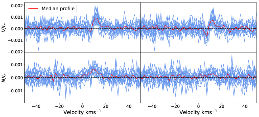
Along with Stokes and profiles, we computed the “Null profile”, which is a powerful diagnostic tool to determine the noise level of the LSD output and whether a spurious polarisation signal is present in the observations (Donati et al., 1997; Bagnulo et al., 2009). As shown in Fig. 1, the Null profile contains a positive signal at line centre (9.6 km s-1), and reflects in a vertical offset of Stokes with respect to a constant null value. Following Folsom et al. (2016), we attributed this signal to an imperfect background subtraction affecting the blue orders of Narval and we removed it by computing LSD profiles using lines in the red part of the spectrum, i.e. larger than 500 nm. Considering a window of 10 km s-1 from line centre that includes both lobes of the Stokes profile, the mean and standard deviation of the Null profile decrease from to and from to , respectively. This procedure does not alter the shape of the Stokes profiles, and removes the vertical offset (see Fig. 1). The S/N of the final profiles ranges between 1600 and 2600.
In the following, the observations are phased according to the ephemeris
| (1) |
where we used the first collected observation date as reference, Prot is the stellar rotation period found using ZDI (see Sec. 5), and is the rotation cycle.
3 Longitudinal magnetic field
The longitudinal field (Bl) is sensitive to the appearance of magnetic regions on the visible stellar hemisphere, which is modulated by the stellar rotation period (Prot). As a result, we can generally apply a standard periodogram analysis to Bl time series in order to find Prot (Hébrard et al., 2016; Petit et al., 2021; Carmona et al., 2023).
Previous studies extracted a stellar rotation period of 39.90.8 d from chromospheric activity indexes time series (Suárez Mascareño et al., 2015; dos Santos et al., 2019) and 44.090.08 d from photometric data sets (Bourrier et al., 2018). Recently, Kumar & Fares (2023) analysed GJ 436’s spectra obtained with HARPS and Narval and, by computing time series of activity indexes such as CaII and H, found a significant (the false-alarm probability, i.e. FAP, was less than 0.1%) periodogram peak at and d, respectively. The Narval data set used by Kumar & Fares (2023) was the same one employed in this work.
We followed Donati et al. (1997) to compute the disk-averaged, line-of-sight-projected stellar magnetic field as the first-order moment of a Stokes profile
| (2) |
where (in nm) and are the normalisation wavelength and Landé factor of the LSD profiles, is the continuum level, is the radial velocity in the star’s rest frame and the speed of light in vacuum (both in km s-1).
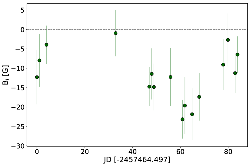
We used a normalisation wavelength and Landé factor of 700 nm and 1.1976, respectively, and performed the integration within 10 km s-1 from line centre at around 9.6 km s-1. The Bl time series is illustrated in Fig. 2, with all values featuring a negative sign.The mean value is 12 G and both the dispersion and mean error bar are 6 G.
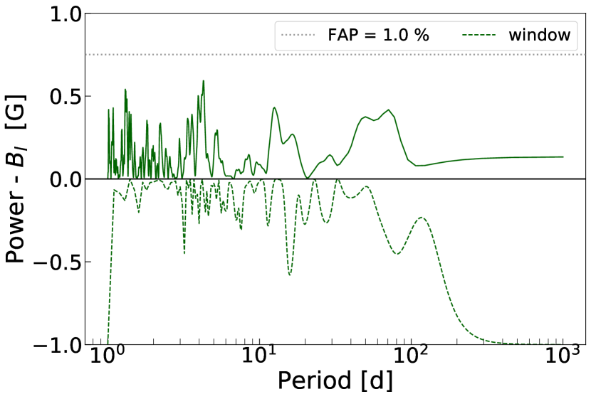
Fig. 2 shows the application of a Generalised Lomb-Scargle periodogram (Zechmeister & Kürster, 2009) to the entire 2016 time series. We do not report any dominant periodicity, the FAP being systematically higher than 1%. The highest peaks are around 4, 15, and 70 d, but they are probably generated by the sparse sampling of our observations, as illustrated by the window function.
4 Gaussian Process Regression
We performed a quasi-periodic Gaussian Process (GP; Haywood et al. 2014) fit to the longitudinal field curve, since this model is more flexible than the standard sine function used in the Lomb-Scargle analysis. In fact, the GP model accounts for the evolution of the magnetic field and its variability (Aigrain & Foreman-Mackey, 2022). Formally, we used the quasi-periodic covariance function
| (3) |
where is a Kronecker delta, and are the hyperparameters of the model: is the amplitude of the curve in G, is the evolution timescale in d (it expresses how rapidly the model evolves), is the recurrence timescale (i.e., Prot), and is the smoothness factor (controlling the harmonic structure of the curve). We added an additional hyperparameter to account for the excess of uncorrelated noise (). In practice we used the cpnest package (Del Pozzo & Veitch, 2022) which performs Bayesian inference via nested sampling algorithm (Skilling, 2004).
| Hyperparameter | Prior | Best fit value |
|---|---|---|
| Amplitude [G] () | ||
| Decay time [d] () | ||
| Prot [d] () | ||
| Smoothness () | ||
| Uncorrelated noise [G] () |
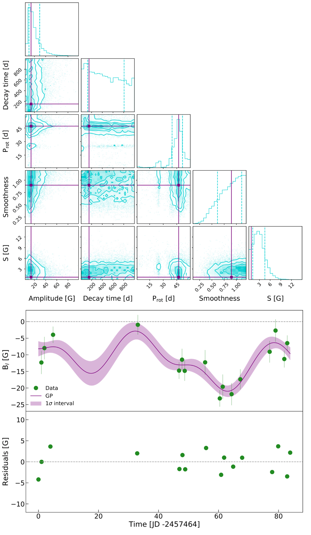
The results are reported in Table 2 and showed in Fig. 3. We applied uniform priors to all five hyperparameters, and allowed the search within realistic boundaries. The model fits the data to a of 0.6, likely indicating that our formal error bars are overestimated. Following Donati et al. (2023), we rescaled the error bars by a factor of 2 to fit the data at , while keeping the excess of uncorrelated noise consistent with zero (see Fig. 3). The GP model is characterised by smooth oscillations (i.e., =1.1), with an amplitude of 12 G and a stellar rotation period of 46.6 d, which is in agreement with the value estimated in the literature within error bars (Suárez Mascareño et al., 2015; Bourrier et al., 2018; Kumar & Fares, 2023). The dispersion of the residuals is 2.5 G, i.e. slightly lower than the rescaled error bars.
For Prot, using a uniform prior between 1 and 100 d results in a marginalised posterior distribution with three peaks, around 20 d, 40 d and 80 d, with the latter being the highest peak. From the Lomb-Scargle analysis presented in Fig. 2, we observe that the observing window function features a broad peak at 80 d, hence we can exclude it from being the genuine rotation period of the star. If we lower the uniform prior boundary to 60 d, the marginalised posterior distribution exhibits a maximum at 46.6 d.
We also notice that the evolution time scale is not constrained by the GP. This is not surprising given the short (i.e. 80 d) time span of our observations. We therefore fixed to either 200 or 300 d, following the results of starspots lifetime analysis carried out by Giles et al. (2017), and performed a 4-hyperparameters GP fit, but the results were only marginally different than those obtained with a 5-hyperparameters GP. We also attempted an analogous test fixing a decay time of 470 d, i.e. the active regions timescale reported by Kumar & Fares (2023), but the results did not differ. Finally, a similar conclusion is obtained when fixing both the decay time scale and the smoothness to the values constrained by Martioli et al. (2022) for TOI-1759, which is an M dwarf of similar spectral type as GJ 436. We used 400-600 d and 0.7-0.9 for and , respectively.
Finally, although the GP retrieves the stellar rotation period around the expected value, we note that the error bars of such time scale are large. An alternative option to extract the stellar rotation period is via ZDI optimisation, as outlined in the next section.
5 Zeeman-Doppler Imaging
We reconstructed the large-scale magnetic field at the surface of GJ 436 by means of ZDI. The field is formally described as the sum of a poloidal and toroidal component, both expressed via spherical harmonic decomposition (Donati et al., 2006; Lehmann & Donati, 2022). With ZDI, we synthesise and adjust Stokes profiles in an iterative fashion, until a maximum-entropy solution at a fixed reduced is achieved (Skilling & Bryan, 1984; Donati & Brown, 1997; Folsom et al., 2018). The iterative process aims to fit the spherical harmonics coefficients , , and (with and the degree and order of the mode, respectively).
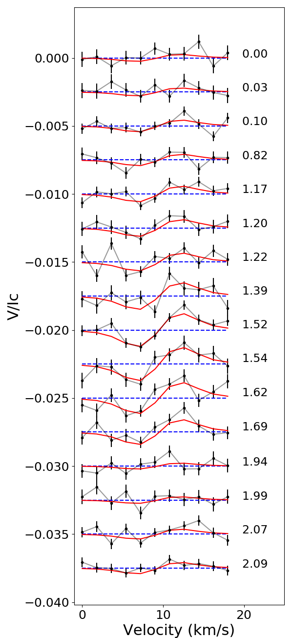
We optimised the input stellar rotation period following the method described in Petit et al. (2002) and Morin et al. (2008). Basically, we sought the value minimising the distribution at a fixed entropy (information content) over a grid of possible values between 2 and 100 d. We found P d, which is compatible with the GP model estimate in Sec. 4, as well as with literature estimates (Bourrier et al., 2018; Kumar & Fares, 2023). For the other input parameters, we adopted an inclination of 40∘ and an equatorial projected velocity () of 0.33 km s-1 (Bourrier et al., 2022). We further assumed solid body rotation, a linear limb darkening law with a -band coefficient of 0.6964 (Claret & Bloemen, 2011), and the maximum degree of harmonic expansion , to match the spatial resolution determined by the of the star. The Narval Stokes V time series is shown in Fig. 4.
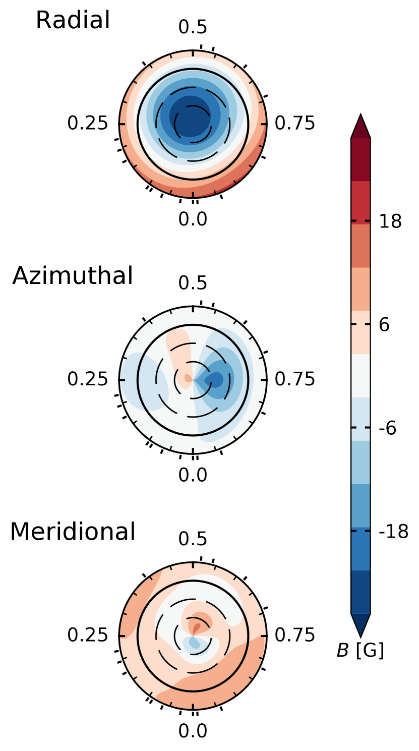
The model Stokes profiles are fit down to , from an initial value of 2.24. The target represents the best value that avoids underfitting and overfitting of the Stokes shape, resulting in a, e.g., weaker field or spurious magnetic features, respectively. The magnetic map is illustrated in Fig. 5 and its properties are listed in Table 3. The mean magnetic field strength is B 16 G, with the poloidal component accounting for 96% of the magnetic energy. The dipolar and quadrupolar modes store 90% and 8% energy, and the field is mostly axisymmetric (79%), with an obliquity of its axis of 15.5∘.
Zeeman Doppler Imaging does not provide error bars on the reconstructed maps, and thus on field characteristics. We estimated variation bars on the field characteristics following the method of Mengel et al. (2016) and Fares et al. (2017). We reconstructed magnetic maps for the input parameters (inclination, , and Prot) by varying each of them within their error bars. The variation bars reported in Table 3 correspond to the maximum difference of field characteristics between the map with the optimised set of input parameters, and the ones considering the error bars on the input parameters. We also reconstructed the magnetic field topology using Prot = 44.09 d as input (Bourrier et al., 2018). The target was adjusted to a larger value of 1.18, but the final map was consistent with the one presented in Fig. 5 within variation bars.
| Bmean [G] | 15.9 |
|---|---|
| Bmax [G] | 30.9 |
| Bpol [%] | 96.4 |
| Btor [%] | 3.6 |
| Bdip [%] | 90.4 |
| Bquad [%] | 7.8 |
| Boct [%] | 1.7 |
| Baxisym [%] | 78.7 |
| Obliquity [∘] | 15.5 |
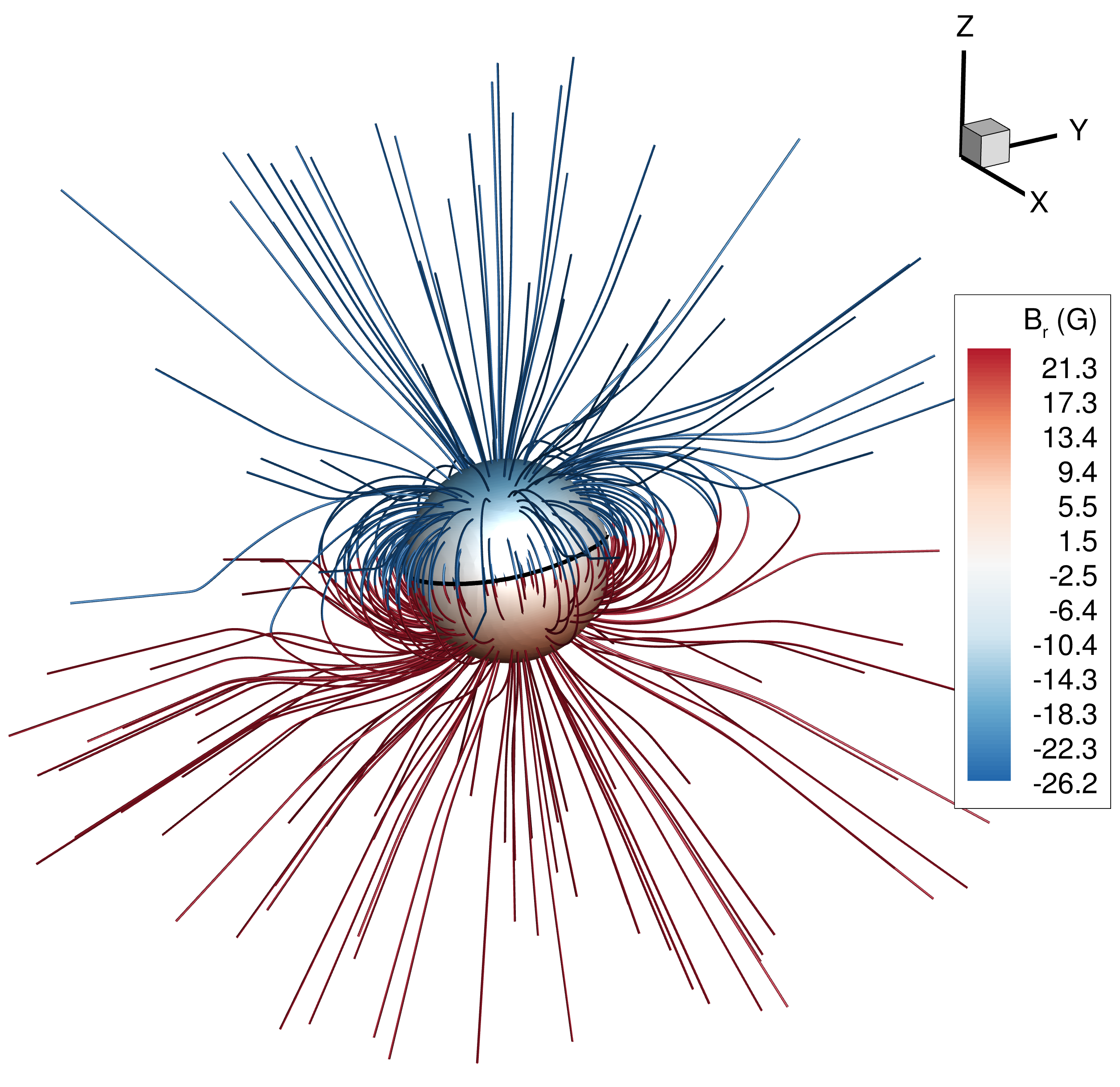
For illustration, Fig. 6 shows an extrapolation of the surface field of the star. We used a potential field source surface method (e.g. Jardine et al., 2002), adopting a source surface at a distance of 4 stellar radii – beyond this distance, the field lines are fully open and purely radial. Using this extrapolation method, we found that at the orbital distance of GJ 436 b (0.028 au; Butler et al. 2004), the radial magnetic field ranges from G to G, with the negative value representing an inward radial field and the positive value an outward radial field. In a follow up study, we will perform stellar wind modelling and provide more detailed predictions of the characteristics of the wind environment (including its embedded magnetic field) at the orbit of GJ 436 b.
6 Discussion and conclusions
In this paper, we presented the analysis of the large-scale magnetic field of the exoplanet host star GJ 436. This will serve as input for the stellar wind and star-planet interaction analysis which will be presented in a future paper (Vidotto et al., subm.). The main goal is to understand stellar environments around M dwarfs, which is relevant for both exoplanet searches and habitability assessment frameworks (Vidotto et al., 2013; O’Malley-James & Kaltenegger, 2019; Lingam & Loeb, 2019). Ultimately, this will provide insightful feedback on the influence of stellar magnetic fields on planetary atmospheres and habitability, which is of crucial importance for JWST and Ariel, since GJ 436 is in the reference sample of both missions (Edwards & Tinetti, 2022).
We used spectropolarimetric data collected with Narval in 2016, and we computed the longitudinal magnetic field from the time series of circularly polarised spectra. To the same time series, we applied tomographic inversion (i.e., Zeeman-Doppler Imaging) to reconstruct a map of the large-scale magnetic field topology. Our conclusions are summarised as follows:
-
1.
The longitudinal field (Bl) spans between 0.9 and 23.1 G, with a median error bar of 6 G. Such field strength is comparable with that of other M dwarfs with similar spectral types and rotation periods.
-
2.
A periodicity analysis by means of generalised Lomb-Scargle periodogram applied to the Bl time series did not highlight any specific periodicity, similarly to the activity indexes analysis of Kumar & Fares (2023). More specifically, we did not retrieve the expected rotation period of about 40 d, but observe different insignificant (FAP¿1%) peaks mostly associated with the observational window. We found (Ricker et al., 2015) observations of GJ 436 collected in 2020 and 2022, but in both cases the observing window is shorter than the expected rotation period of the star, hence they cannot be used to constrain such parameter.
-
3.
The GP regression analysis applied to the Bl time series produces a smooth model characterised by a rotation period of d. From the optimisation of stellar input parameters with Zeeman-Doppler Imaging, we were able to infer P d. Both values are in agreement with literature estimates within uncertainties.
-
4.
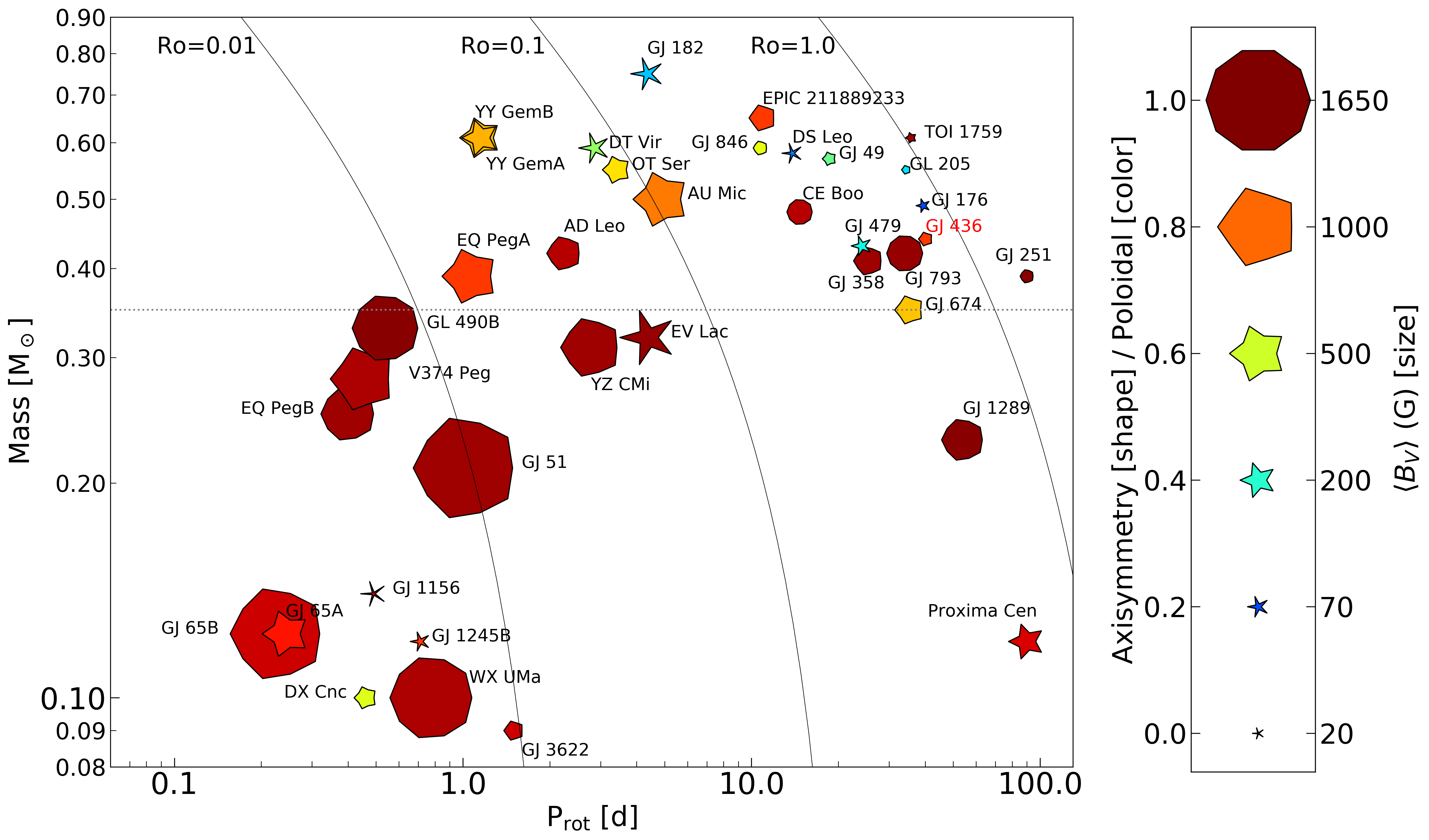
The application of Zeeman-Doppler Imaging to the Stokes time series revealed a simple field configuration, characterised by a poloidal, mainly dipolar and axisymmetric topology, with a mean magnetic field strength of 16 G. This simple geometry is in accordance with other stars of similar spectral type, mass and rotation period, i.e. GJ 205 (Hébrard et al., 2016; Cortés-Zuleta et al., 2023) and TOI-1759 (Martioli et al., 2022), as can be seen in Fig. 7.
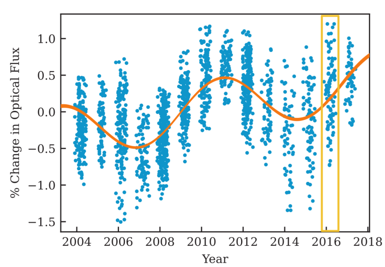
GJ 436 is known to have an activity cycle: Lothringer et al. (2018) analysed 14 years of photometric data (in Strömgren and filters) between 2004 and 2018, and reported a 7.4 yr cycle, which was then re-analysed by Loyd et al. (2023) who consistently found a 7.75 yr cycle. Moreover, a similar time scale between 5 and 7 yr was obtained by Kumar & Fares (2023) from time series of chromospheric activity indexes (H, NaI, and CaII H&K), spanning 14 yr. This in agreement with what is expected for M dwarfs from radial velocity exoplanet searches (Gomes da Silva et al., 2012) and photometric surveys (Suárez Mascareño et al., 2016, 2018) for M dwarfs of similar spectral type.
In this light, it is interesting to place the magnetic field map we reconstructed along the track of the activity cycle. Our observations were collected in 2016 (see Table 1), meaning that our ZDI map portrays the magnetic field during an ascending phase of the cycle (i.e. towards photometric maximum), as shown in the yellow box in Fig. 8. This advocates for additional spectropolarimetric monitoring of GJ 436, in order to ideally reconstruct a ZDI map during cycle minimum and maximum, and catch whether the magnetic field undergoes polarity reversals like for the Sun (Sanderson et al., 2003; Lehmann et al., 2021), and other stars and other cool stars (e.g. Boo Fares et al. 2009; Mengel et al. 2016; Jeffers et al. 2018 and 61 Cyg Boro Saikia et al. 2016). If we assume P yr, we predict the next photometric minimum to be around 2030, whereas the next maximum to be around mid 2026. Monitoring the secular evolution of the large-scale field of GJ 436 would be an essential ingredient to interpret the observed signatures of star-planet interactions. Indeed, magnetic cycles modulate the radiation output of stars (Yeo et al., 2014; Hazra et al., 2020), therefore providing a temporal modulation of planetary atmospheric erosion.
Acknowledgements.
We thank the anonymous referee for the fruitful review of this work. We acknowledge funding from the French National Research Agency (ANR) under contract number ANR-18-CE31-0019 (SPlaSH). RF acknowledges support from the United Arab Emirates University (UAEU) startup grant number G00003269. This work has been carried out within the framework of the NCCR PlanetS supported by the Swiss National Science Foundation under grants 51NF40182901 and 51NF40205606. This project has received funding from the European Research Council (ERC) under the European Union’s Horizon 2020 research and innovation programme (projects Spice Dune and ASTROFLOW, grant agreements No 947634 and 817540). This work has made use of the VALD database, operated at Uppsala University, the Institute of Astronomy RAS in Moscow, and the University of Vienna; Astropy, 12 a community-developed core Python package for Astronomy (Astropy Collaboration et al., 2013, 2018); NumPy (van der Walt et al., 2011); Matplotlib: Visualization with Python (Hunter, 2007); SciPy (Virtanen et al., 2020) and PyAstronomy (Czesla et al., 2019).References
- Aigrain & Foreman-Mackey (2022) Aigrain, S. & Foreman-Mackey, D. 2022, arXiv e-prints, arXiv:2209.08940
- Allan & Vidotto (2019) Allan, A. & Vidotto, A. A. 2019, MNRAS, 490, 3760
- Astropy Collaboration et al. (2018) Astropy Collaboration, Price-Whelan, A. M., Sipőcz, B. M., et al. 2018, AJ, 156, 123
- Astropy Collaboration et al. (2013) Astropy Collaboration, Robitaille, T. P., Tollerud, E. J., et al. 2013, A&A, 558, A33
- Attia et al. (2021) Attia, O., Bourrier, V., Eggenberger, P., et al. 2021, A&A, 647, A40
- Bagnulo et al. (2009) Bagnulo, S., Landolfi, M., Landstreet, J. D., et al. 2009, PASP, 121, 993
- Beaugé & Nesvorný (2013) Beaugé, C. & Nesvorný, D. 2013, ApJ, 763, 12
- Bellotti et al. (2022) Bellotti, S., Petit, P., Morin, J., et al. 2022, A&A, 657, A107
- Beust et al. (2012) Beust, H., Bonfils, X., Montagnier, G., Delfosse, X., & Forveille, T. 2012, A&A, 545, A88
- Boro Saikia et al. (2016) Boro Saikia, S., Jeffers, S. V., Morin, J., et al. 2016, A&A, 594, A29
- Boro Saikia et al. (2018) Boro Saikia, S., Marvin, C. J., Jeffers, S. V., et al. 2018, A&A, 616, A108
- Bourrier et al. (2015) Bourrier, V., Ehrenreich, D., & Lecavelier des Etangs, A. 2015, A&A, 582, A65
- Bourrier et al. (2016) Bourrier, V., Lecavelier des Etangs, A., Ehrenreich, D., Tanaka, Y. A., & Vidotto, A. A. 2016, A&A, 591, A121
- Bourrier et al. (2018) Bourrier, V., Lovis, C., Beust, H., et al. 2018, Nature, 553, 477
- Bourrier et al. (2022) Bourrier, V., Zapatero Osorio, M. R., Allart, R., et al. 2022, A&A, 663, A160
- Butler et al. (2004) Butler, R. P., Vogt, S. S., Marcy, G. W., et al. 2004, ApJ, 617, 580
- Carmona et al. (2023) Carmona, A., Delfosse, X., Bellotti, S., et al. 2023, A&A, 674, A110
- Carolan et al. (2021) Carolan, S., Vidotto, A. A., Villarreal D’Angelo, C., & Hazra, G. 2021, MNRAS, 500, 3382
- Chabrier & Baraffe (1997) Chabrier, G. & Baraffe, I. 1997, A&A, 327, 1039
- Claret & Bloemen (2011) Claret, A. & Bloemen, S. 2011, A&A, 529, A75
- Cortés-Zuleta et al. (2023) Cortés-Zuleta, P., Boisse, I., Klein, B., et al. 2023, A&A, 673, A14
- Czesla et al. (2019) Czesla, S., Schröter, S., Schneider, C. P., et al. 2019, PyA: Python astronomy-related packages, Astrophysics Source Code Library, record ascl:1906.010
- Davis & Wheatley (2009) Davis, T. A. & Wheatley, P. J. 2009, MNRAS, 396, 1012
- Del Pozzo & Veitch (2022) Del Pozzo, W. & Veitch, J. 2022, CPNest: Parallel nested sampling, Astrophysics Source Code Library, record ascl:2205.021
- Donati (2003) Donati, J. F. 2003, in Astronomical Society of the Pacific Conference Series, Vol. 307, Solar Polarization, ed. J. Trujillo-Bueno & J. Sanchez Almeida, 41
- Donati & Brown (1997) Donati, J. F. & Brown, S. F. 1997, A&A, 326, 1135
- Donati et al. (2023) Donati, J. F., Cristofari, P. I., Finociety, B., et al. 2023, MNRAS[arXiv:2304.09642]
- Donati et al. (2006) Donati, J. F., Howarth, I. D., Jardine, M. M., et al. 2006, MNRAS, 370, 629
- Donati et al. (2008) Donati, J. F., Morin, J., Petit, P., et al. 2008, MNRAS, 390, 545
- Donati et al. (1997) Donati, J. F., Semel, M., Carter, B. D., Rees, D. E., & Collier Cameron, A. 1997, MNRAS, 291, 658
- dos Santos et al. (2019) dos Santos, L. A., Ehrenreich, D., Bourrier, V., et al. 2019, A&A, 629, A47
- Edwards & Tinetti (2022) Edwards, B. & Tinetti, G. 2022, AJ, 164, 15
- Ehrenreich et al. (2015) Ehrenreich, D., Bourrier, V., Wheatley, P. J., et al. 2015, Nature, 522, 459
- Ehrenreich & Désert (2011) Ehrenreich, D. & Désert, J. M. 2011, A&A, 529, A136
- Fares et al. (2017) Fares, R., Bourrier, V., Vidotto, A. A., et al. 2017, MNRAS, 471, 1246
- Fares et al. (2009) Fares, R., Donati, J. F., Moutou, C., et al. 2009, MNRAS, 398, 1383
- Fares et al. (2013) Fares, R., Moutou, C., Donati, J. F., et al. 2013, MNRAS, 435, 1451
- Folsom et al. (2018) Folsom, C. P., Bouvier, J., Petit, P., et al. 2018, MNRAS, 474, 4956
- Folsom et al. (2016) Folsom, C. P., Petit, P., Bouvier, J., et al. 2016, MNRAS, 457, 580
- Fuhrmeister et al. (2023) Fuhrmeister, B., Czesla, S., Perdelwitz, V., et al. 2023, A&A, 670, A71
- Gaia Collaboration et al. (2021) Gaia Collaboration, Smart, R. L., Sarro, L. M., et al. 2021, A&A, 649, A6
- Giles et al. (2017) Giles, H. A. C., Collier Cameron, A., & Haywood, R. D. 2017, MNRAS, 472, 1618
- Gillon et al. (2007) Gillon, M., Pont, F., Demory, B. O., et al. 2007, A&A, 472, L13
- Gomes da Silva et al. (2012) Gomes da Silva, J., Santos, N. C., Bonfils, X., et al. 2012, A&A, 541, A9
- Günther et al. (2020) Günther, M. N., Zhan, Z., Seager, S., et al. 2020, AJ, 159, 60
- Gustafsson et al. (2008) Gustafsson, B., Edvardsson, B., Eriksson, K., et al. 2008, A&A, 486, 951
- Haywood et al. (2014) Haywood, R. D., Collier Cameron, A., Queloz, D., et al. 2014, MNRAS, 443, 2517
- Hazra et al. (2022) Hazra, G., Vidotto, A. A., Carolan, S., Villarreal D’Angelo, C., & Manchester, W. 2022, MNRAS, 509, 5858
- Hazra et al. (2020) Hazra, G., Vidotto, A. A., & D’Angelo, C. V. 2020, MNRAS, 496, 4017
- Hébrard et al. (2016) Hébrard, É. M., Donati, J. F., Delfosse, X., et al. 2016, MNRAS, 461, 1465
- Hunter (2007) Hunter, J. D. 2007, Computing in Science and Engineering, 9, 90
- Jardine et al. (2002) Jardine, M., Collier Cameron, A., & Donati, J. F. 2002, MNRAS, 333, 339
- Jeffers et al. (2018) Jeffers, S. V., Mengel, M., Moutou, C., et al. 2018, MNRAS, 479, 5266
- Kavanagh et al. (2021) Kavanagh, R. D., Vidotto, A. A., Klein, B., et al. 2021, MNRAS, 504, 1511
- Kavanagh et al. (2022) Kavanagh, R. D., Vidotto, A. A., Vedantham, H. K., et al. 2022, MNRAS, 514, 675
- Ketzer & Poppenhaeger (2023) Ketzer, L. & Poppenhaeger, K. 2023, MNRAS, 518, 1683
- Khodachenko et al. (2019) Khodachenko, M. L., Shaikhislamov, I. F., Lammer, H., et al. 2019, ApJ, 885, 67
- Klein et al. (2021) Klein, B., Donati, J.-F., Moutou, C., et al. 2021, MNRAS, 502, 188
- Kochukhov & Lavail (2017) Kochukhov, O. & Lavail, A. 2017, ApJ, 835, L4
- Kochukhov et al. (2010) Kochukhov, O., Makaganiuk, V., & Piskunov, N. 2010, A&A, 524, A5
- Kochukhov & Shulyak (2019) Kochukhov, O. & Shulyak, D. 2019, ApJ, 873, 69
- Konings et al. (2022) Konings, T., Baeyens, R., & Decin, L. 2022, A&A, 667, A15
- Kulow et al. (2014) Kulow, J. R., France, K., Linsky, J., & Loyd, R. O. P. 2014, ApJ, 786, 132
- Kumar & Fares (2023) Kumar, M. & Fares, R. 2023, MNRAS, 518, 3147
- Lammer et al. (2003) Lammer, H., Selsis, F., Ribas, I., et al. 2003, ApJ, 598, L121
- Lavie et al. (2017) Lavie, B., Ehrenreich, D., Bourrier, V., et al. 2017, A&A, 605, L7
- Lecavelier Des Etangs (2007) Lecavelier Des Etangs, A. 2007, A&A, 461, 1185
- Lehmann & Donati (2022) Lehmann, L. T. & Donati, J. F. 2022, MNRAS, 514, 2333
- Lehmann et al. (2021) Lehmann, L. T., Hussain, G. A. J., Vidotto, A. A., Jardine, M. M., & Mackay, D. H. 2021, MNRAS, 500, 1243
- Lingam & Loeb (2019) Lingam, M. & Loeb, A. 2019, International Journal of Astrobiology, 18, 527
- Llama et al. (2013) Llama, J., Vidotto, A. A., Jardine, M., et al. 2013, MNRAS, 436, 2179
- Lothringer et al. (2018) Lothringer, J. D., Benneke, B., Crossfield, I. J. M., et al. 2018, AJ, 155, 66
- Louca et al. (2023) Louca, A. J., Miguel, Y., Tsai, S.-M., et al. 2023, MNRAS, 521, 3333
- Loyd et al. (2023) Loyd, R. O. P., Schneider, P. C., Jackman, J. A. G., et al. 2023, AJ, 165, 146
- Luger et al. (2015) Luger, R., Barnes, R., Lopez, E., et al. 2015, Astrobiology, 15, 57
- Lundkvist et al. (2016) Lundkvist, M. S., Kjeldsen, H., Albrecht, S., et al. 2016, Nature Communications, 7, 11201
- Martioli et al. (2022) Martioli, E., Hébrard, G., Fouqué, P., et al. 2022, A&A, 660, A86
- Mazeh et al. (2016) Mazeh, T., Holczer, T., & Faigler, S. 2016, A&A, 589, A75
- Mengel et al. (2016) Mengel, M. W., Fares, R., Marsden, S. C., et al. 2016, MNRAS, 459, 4325
- Mesquita et al. (2021) Mesquita, A. L., Rodgers-Lee, D., & Vidotto, A. A. 2021, MNRAS, 505, 1817
- Morin et al. (2008) Morin, J., Donati, J. F., Petit, P., et al. 2008, MNRAS, 390, 567
- Morin et al. (2010) Morin, J., Donati, J. F., Petit, P., et al. 2010, MNRAS, 407, 2269
- Moutou et al. (2017) Moutou, C., Hébrard, E. M., Morin, J., et al. 2017, MNRAS, 472, 4563
- O’Malley-James & Kaltenegger (2019) O’Malley-James, J. T. & Kaltenegger, L. 2019, MNRAS, 485, 5598
- Owen & Jackson (2012) Owen, J. E. & Jackson, A. P. 2012, MNRAS, 425, 2931
- Penz et al. (2008) Penz, T., Micela, G., & Lammer, H. 2008, A&A, 477, 309
- Petit et al. (2005) Petit, P., Donati, J. F., Aurière, M., et al. 2005, MNRAS, 361, 837
- Petit et al. (2002) Petit, P., Donati, J. F., & Collier Cameron, A. 2002, MNRAS, 334, 374
- Petit et al. (2021) Petit, P., Folsom, C. P., Donati, J. F., et al. 2021, A&A, 648, A55
- Petit et al. (2014) Petit, P., Louge, T., Théado, S., et al. 2014, PASP, 126, 469
- Phan-Bao et al. (2009) Phan-Bao, N., Lim, J., Donati, J.-F., Johns-Krull, C. M., & Martín, E. L. 2009, ApJ, 704, 1721
- Ribas et al. (2005) Ribas, I., Guinan, E. F., Güdel, M., & Audard, M. 2005, ApJ, 622, 680
- Ricker et al. (2015) Ricker, G. R., Winn, J. N., Vanderspek, R., et al. 2015, Journal of Astronomical Telescopes, Instruments, and Systems, 1, 014003
- Rodgers-Lee et al. (2023) Rodgers-Lee, D., Rimmer, P. B., Vidotto, A. A., et al. 2023, MNRAS, 521, 5880
- Rosenthal et al. (2021) Rosenthal, L. J., Fulton, B. J., Hirsch, L. A., et al. 2021, ApJS, 255, 8
- Ryabchikova et al. (2015) Ryabchikova, T., Piskunov, N., Kurucz, R. L., et al. 2015, Phys. Scr, 90, 054005
- Sanderson et al. (2003) Sanderson, T. R., Appourchaux, T., Hoeksema, J. T., & Harvey, K. L. 2003, Journal of Geophysical Research (Space Physics), 108, 1035
- Saur et al. (2013) Saur, J., Grambusch, T., Duling, S., Neubauer, F. M., & Simon, S. 2013, A&A, 552, A119
- Segura et al. (2010) Segura, A., Walkowicz, L. M., Meadows, V., Kasting, J., & Hawley, S. 2010, Astrobiology, 10, 751
- Semel (1989) Semel, M. 1989, A&A, 225, 456
- Skilling (2004) Skilling, J. 2004, in American Institute of Physics Conference Series, Vol. 735, Bayesian Inference and Maximum Entropy Methods in Science and Engineering: 24th International Workshop on Bayesian Inference and Maximum Entropy Methods in Science and Engineering, ed. R. Fischer, R. Preuss, & U. V. Toussaint, 395–405
- Skilling & Bryan (1984) Skilling, J. & Bryan, R. K. 1984, MNRAS, 211, 111
- Suárez Mascareño et al. (2016) Suárez Mascareño, A., Rebolo, R., & González Hernández, J. I. 2016, A&A, 595, A12
- Suárez Mascareño et al. (2015) Suárez Mascareño, A., Rebolo, R., González Hernández, J. I., & Esposito, M. 2015, MNRAS, 452, 2745
- Suárez Mascareño et al. (2018) Suárez Mascareño, A., Rebolo, R., González Hernández, J. I., et al. 2018, A&A, 612, A89
- Tilley et al. (2019) Tilley, M. A., Segura, A., Meadows, V., Hawley, S., & Davenport, J. 2019, Astrobiology, 19, 64
- Turnpenney et al. (2018) Turnpenney, S., Nichols, J. D., Wynn, G. A., & Burleigh, M. R. 2018, ApJ, 854, 72
- van der Walt et al. (2011) van der Walt, S., Colbert, S. C., & Varoquaux, G. 2011, Computing in Science and Engineering, 13, 22
- VanderPlas (2018) VanderPlas, J. T. 2018, The Astrophysical Journal Supplement Series, 236, 16
- Vidal-Madjar et al. (2003) Vidal-Madjar, A., Lecavelier des Etangs, A., Désert, J. M., et al. 2003, Nature, 422, 143
- Vidotto & Bourrier (2017) Vidotto, A. A. & Bourrier, V. 2017, MNRAS, 470, 4026
- Vidotto et al. (2014a) Vidotto, A. A., Gregory, S. G., Jardine, M., et al. 2014a, MNRAS, 441, 2361
- Vidotto et al. (2013) Vidotto, A. A., Jardine, M., Morin, J., et al. 2013, A&A, 557, A67
- Vidotto et al. (2014b) Vidotto, A. A., Jardine, M., Morin, J., et al. 2014b, MNRAS, 438, 1162
- Villarreal D’Angelo et al. (2018) Villarreal D’Angelo, C., Esquivel, A., Schneiter, M., & Sgró, M. A. 2018, MNRAS, 479, 3115
- Villarreal D’Angelo et al. (2021) Villarreal D’Angelo, C., Vidotto, A. A., Esquivel, A., Hazra, G., & Youngblood, A. 2021, MNRAS, 501, 4383
- Virtanen et al. (2020) Virtanen, P., Gommers, R., Burovski, E., et al. 2020, scipy/scipy: SciPy 1.5.3
- Wright et al. (2018) Wright, N. J., Newton, E. R., Williams, P. K. G., Drake, J. J., & Yadav, R. K. 2018, MNRAS, 479, 2351
- Yeo et al. (2014) Yeo, K. L., Krivova, N. A., & Solanki, S. K. 2014, Space Sci. Rev., 186, 137
- Zacharias et al. (2012) Zacharias, N., Finch, C. T., Girard, T. M., et al. 2012, VizieR Online Data Catalog, I/322A
- Zarka (1998) Zarka, P. 1998, J. Geophys. Res., 103, 20159
- Zechmeister & Kürster (2009) Zechmeister, M. & Kürster, M. 2009, A&A, 496, 577
- Zeeman (1897) Zeeman, P. 1897, Nature, 55, 347