Chemical bond analysis for the entire periodic table: Energy Decomposition and Natural Orbitals for Chemical Valence in the Four-Component Relativistic Framework

Abstract

Chemical bonding is a ubiquitous concept in chemistry and it provides a common basis for experimental and theoretical chemists to explain and predict the structure, stability and reactivity of chemical species. Among others, the Energy Decomposition Analysis (EDA, also known as the Extended Transition State method) in combination with Natural Orbitals for Chemical Valence (EDA-NOCV) is a very powerful tool for the analysis of the chemical bonds based on a charge and energy decomposition scheme within a common theoretical framework. While the approach has been applied in a variety of chemical contexts, the current implementations of the EDA-NOCV scheme include relativistic effects only at scalar level, so simply neglecting the spin-orbit coupling effects and de facto limiting its applicability. In this work, we extend the EDA-NOCV method to the relativistic four-component Dirac-Kohn-Sham theory that variationally accounts for spin-orbit coupling. Its correctness and numerical stability have been demonstrated in the case of simple molecular systems, where the relativistic effects play a negligible role, by comparison with the implementation available in the ADF modelling suite (using the non-relativistic Hamiltonian and the scalar ZORA approximation). As an illustrative example we analyse the metal-ethylene coordination bond in the group 6-element series (CO)₅TM-C₂H₄, with TM =Cr, Mo, W, Sg, where relativistic effects are likely to play an increasingly important role as one moves down the group. The method provides a clear measure (also in combination with the CD analysis) of the donation and back-donation components in coordination bonds, even when relativistic effects, including spin-orbit coupling, are crucial for understanding the chemical bond involving heavy and superheavy atoms.

1 Introduction

In recent decades, several approaches, mainly in theoretical chemistry, have been introduced to analyse and characterise chemical bonding. These can be divided into two main groups: i) methods mainly focusing on the decomposition of the binding energy into ’chemically meaningful’ contributions[67, 57, 56, 106, 55] and ii) methods that mainly focus on wave function or electron density analysis[4, 5, 3, 42, 25, 86, 8, 68, 27, 45, 11]. As a matter of fact, a chemical bond is not a well-defined quantum mechanical observable [87] and so it is not surprising that discussions about the nature of chemical bonds typically lead to disputes and misunderstandings. So when designing, developing or applying a theoretical method for analysing a chemical bond, it can be useful to recall Coulson’s perspective[26] which he expressed in a lecture in 1952: “Sometimes it seems to me that a bond between two atoms has become so real, so tangible, so friendly, that I can almost see it. And then I awake with a little shock: for a chemical bond is not a real thing: it does not exist: no one has ever seen it, no- one ever can. It is a figment of our own imagination…” and also “it is a most convenient fiction, which, as we have seen, is convenient both to experimental and theoretical chemists”. If the fundamental theory of quantum mechanics does not help to design unambiguous definitions for chemical bonds, we believe that an important criterion for assessing the validity of a model for chemical bonds lies in its predictive ability within the chemical space. [87] For a critical analysis of the most common bonding models, and the quantum mechanical description of chemical bonds, we refer the reader to the comprehensive review by Frenking et al. [105], which also includes a description of the main theoretical methods available today for bonding analysis. For an overview of the physical nature of chemical bonding, including the latest computational approaches, we refer the reader to a very recent collection of articles [34].

Among other methods available in the literature, energy decomposition analysis (EDA), originally developed by Morokuma [57] and by Ziegler and Rauk [106] and also known as the Extended Transition State Method (ETS), combined [62, 63] with the original density partitioning method Natural Orbitals for the Chemical Valence (NOCV) of Mitoraj and Michalak [66, 64] represents a very powerful method that bridges the gap between elementary quantum mechanics and a conceptually simple interpretation of the nature of chemical bonds. The method, known as EDA-NOCV (or ETS-NOCV), has become an important tool for the analysis of bonds. Indeed, it takes into account different types of physical interactions that contribute to the experimentally observable bond dissociation energy. In particular, this approach is able to decompose the orbital relaxation energy into NOCV pairwise contributions that can be associated with a particular electronic deformation density. The latter can be visualised to characterise the interaction. Furthermore, the NOCV distribution can often be correlated with simple chemical concepts, such as for instance the Dewar-Chatt-Duncanson (DCD) bonding model for coordination chemistry. For a detailed and critical overview of the EDA-NOCV method, and its most common applications, we refer the interested reader to Ref. [104]

Some of us have shown that the rearrangement of electron density associated with the NOCV orbitals pair can be analysed quantitatively by using the so-called charge-displacement (CD) analysis[11]. The method, also known as NOCV/CD, [16, 18] is based on the partial progressive integration of the rearrangement of electron density that occurs during bond formation and is associated with the NOCV partitioning of orbital relaxation. The resulting approach has been applied to quantify the donation and back-donation components of the DCD model, which can be disentangled and brought into very close correlation with experimental observations [15, 24, 2, 17]. The method has been also applied to molecular systems without symmetry constraints, [16, 61, 48, 46] including the analysis of the evolution of a chemical bond between catalyst and substrate along the steps of a reaction pathway [16]. More recently, the EDA-NOCV/CD method has helped us to elucidate the peculiar nature of bonding in coinage metal-aluminyl complexes[92, 94, 95] and their reactivity with carbon dioxide and other small molecules [93, 96, 97].

Despite its wide diffusion, the current implementations of the EDA-NOCV method are limited to non-relativistic Hamiltonians or to include relativistic effects at scalar level, typically using the scalar ZORA approximation, which simply overlooks the spin-orbit coupling effects. However, it is widely recognised that spin-orbit coupling can play an important role not only in spectroscopy, but also in chemical bonding [60, 87, 21] and chemical reactivity. [75, 50, 85, 88, 47, 31, 79, 49] The development of methods which are able to analyse the chemical bonds within a theoretical framework which incorporates spin-orbit coupling effects is of high importance. Among others, [43, 41, 81, 103, 74] the recent work of Senjen et al. [89] where the intrinsic atomic and bond orbitals (IBOs) scheme has been generalised to fully relativistic applications using complex and quaternion spinors as implemented in the DIRAC code [82, 1] goes exactly in this direction. Some of us have extended the NOCV scheme to the Dirac-Kohn-Sham module of the code BERTHA (and in its new Python API, PyBERTHA) and the approach has been successfully used (also in combination with the CD analysis, NOCV/CD) to study chemical bonding and s-d hybridisation in Group 11 M-CN cyanides (M = Cu, Ag and Au) and in Group 11 MH${}_{2}^{-}$ dihydrides (M=Cu, Ag, Au, Rg)[91], superheavy elements interacting with metal clusters, and to characterise weakly bound systems involving astatine [28, 80, 29]. Despite the quantitative measure of the charge transfer (CT) involved upon a bond formation, the NOCV/CD approach, is exclusively focused on the analysis of the rearrangement of the electron density and gives no indication of the different energy terms that contribute to the total energy of the bond. It therefore seems appropriate to extend the NOCV approach already implemented in BERTHA [28] and combine it with EDA. This combined scheme offers the possibility to obtain quantitative information about different energetic terms contributing to the total interaction energy and to assign a well-defined energetic contribution to the rearrangement of the electron density associated with a specific pair of NOCV orbitals. In this paper we present the formalism and implementation of the EDA-NOCV scheme in the context of the relativistic four-component DKS method, where the spin-orbit coupling is variationally included. In Section 2 we recall the essential aspects of the EDA method, including the Extended Transition State method that is used in combination with the NOCV theory (EDA-NOCV). We describe how the scheme can be extended to the Dirac-Kohn-Sham theory as is currently implemented in the DKS module of the BERTHA code[12, 98, 99, 78] taking advantage of the new Python API. In section 3 we present first test calculations to validate the correctness and numerical stability of our new implementation. An application is also reported in order to illustrate the effective usefulness of the approach to analise the coordinative bond in a consistent manner in the whole periodic table. In particular we have investigated the metal-ethylene bond in the full set of the group 6 carbonyl complexes (CO)₅TM-C₂H₄, with TM =Cr, Mo, W and Sg (Seaborgium, element 106), where relativistic effects become increasingly important. Some conclusions and perspectives are drawn in the last Section.

2 Methodology

2.1 Energy Decomposition Analysis and Natural Orbital for the Chemical Valence (EDA-NOCV)

We begin this Section with a brief overview of the EDA scheme in the version originally introduced by Morokuma [57] and successively by Ziegler and Rauk [106] at the Hartree-Fock or Hartree-Fock-Slater level. In the literature, this scheme is also known as the Extended Transition State (ETS) scheme, named after the original work of Ziegler and Rauk [106]. An important impetus for the dissemination of EDA was its development in the context of Kohn-Sham theory and its implementation in the ADF code over many years [14]. More recently, the scheme has been combined with natural orbitals for chemical valence (EDA-NOCV) [65], where the Extended Transition State method was used to decompose the orbital interaction energy in terms of well defined contributions associated with specific NOCV deformation densities that can be visualized and analised to characterize the interaction. For a detailed description, we refer the reader to the original papers [106, 14, 65]. For the sake of clarity, in the following summary of the EDA-NOCV scheme, we attempt to use a notation which is as consistent as possible with that used by Frenking et al. in a recent review article [104] and by Ziegler et al. in the seminal work on ETS-NOCV [65].

The fundamental idea of this energy partition scheme is the decomposition of the total binding energy ($\Delta E$) between two fragments A and B as a sum of well-defined terms. These terms can be defined by assigning intermediate states to the system in the course of bond formation in a kind of stepwise mechanism. Each state can be reached by applying a well-defined mathematical procedure that can be associated with a physically meaningful entity.

At first the total binding energy ($\Delta E$) is split into two main components, $\Delta E_{prep}$ and $\Delta E_{int}$:

$$\Delta E=\Delta E_{prep}+\Delta E_{int}$$ (1)

$\Delta E_{prep}$ is the energy required to bring the fragments A and B from their equilibrium geometry, at their ground electronic configuration, to the geometry they acquire in the compound AB in their valence electronic configuration. Instead, $\Delta E_{int}$ is the instantaneous interaction energy between the two fragments in the molecule. The latter quantity is in turn divided into three terms:

$$\Delta E_{int}=\Delta E_{elstat}+\Delta E_{Pauli}+\Delta E_{orb}$$ (2)

where $\Delta E_{elstat}$ is the electrostatic interaction, $\Delta E_{Pauli}$ is called the Pauli term and $\Delta E_{orb}$ is the orbital interaction term.

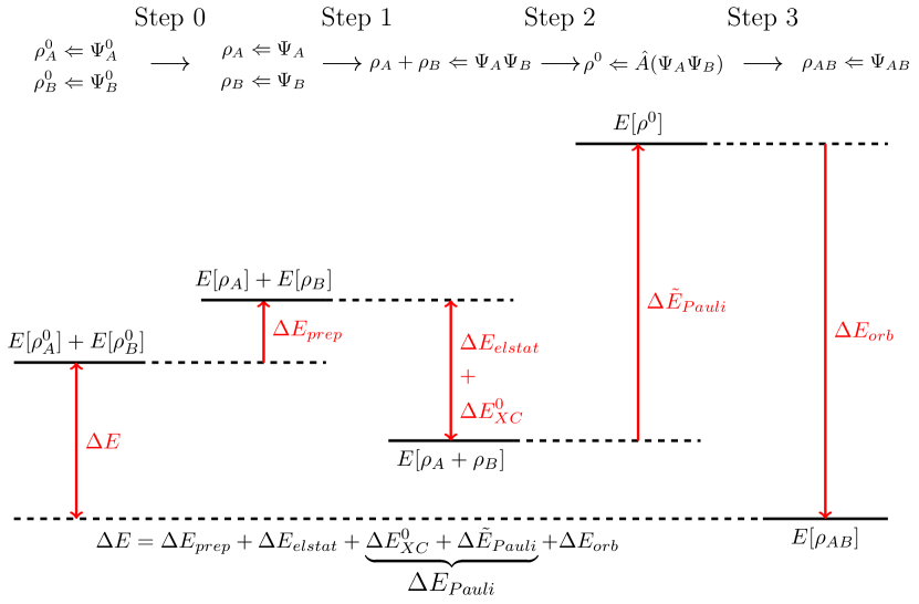
Figure 1: Graphycal stepwise representation of EDA, see text for details.

The graphical illustration of the individual steps at the basis of EDA can be visualized in Figure 1. Initially, the system switches from state 0, which is characterised by the isolated and non-interacting fragments (infinite spatial distance) with well-defined Kohn-Sham determinants ($\Psi_{A}^{0}$ and $\Psi_{B}^{0}$) and electron densities ($\rho_{A}^{0}$ and $\rho_{B}^{0}$). In the first step, the fragments are distorted into the geometry ($\Psi_{A}$ and $\Psi_{B}$) they possess in the final adduct. The energy increases by an amount that corresponds to the definition of the preparation energy mentioned above, $\Delta E_{prep}=E[\rho_{A}]+E[\rho_{B}]-E[\rho_{A}^{0}]-E[\rho_{B}^{0}]$. In the second step, the distorted fragments are moved from infinite distance to their final position, which they occupy in the complex, without changing their densities ($\rho_{A}$ and $\rho_{B}$) and orbitals. The associated change in energy is now given by $E[\rho_{A}+\rho_{B}]-E[\rho_{A}]-E[\rho_{B}]$ which can be easily written as (see Appendix A)

$$E[\rho_{A}+\rho_{B}]-E[\rho_{A}]-E[\rho_{B}]=\Delta E_{elstat}+\Delta E_{XC}^{0}.$$ (3)

$\Delta E_{elstat}$ represents the classical electrostatic interaction between the unperturbed charge distributions ($\rho_{A}$ and $\rho_{B}$) of the prepared fragments when they are brought together at their final positions. The resulting total density is a simple superposition of the fragment densities, and its explicit expression is given by

$$\Delta E_{elstat} = -\sum_{i\in\{A\}}\int\frac{Z_{i}\rho_{B}(r)}{|R_{i}-r|}dr-\sum_{i\in\{B\}}\int\frac{Z_{i}\rho_{A}(r)}{|R_{i}-r|}dr+$$

$$+ \sum_{\begin{subarray}{c}i\in\{A\}\\ j\in\{B\}\end{subarray}}\frac{Z_{i}Z_{j}}{|R_{j}-R_{i}|}+\int\int\frac{(\rho_{A}(r_{1})\rho_{B}(r_{2}))}{|r_{1}-r_{2}|}dr_{1}dr_{2},$$

where the first two terms represent the Coulomb interaction between the charges of the nuclei of fragment A (and B) and the one-electron density of fragment B (and A). Instead, the third term is the classical electrostatic repulsion between the nuclei. Finally, the last term is the Coulomb repulsion between the one-electron densities associated with the two isolated fragments ($\rho_{A}$ and $\rho_{B}$). For the neutral fragments, $\Delta E_{elstat}$ is typically attractive because of a charge penetration that may occur between the two fragments. The term $\Delta E_{XC}^{0}$ in Eq.3, defined as $E_{XC}[\rho_{A}+\rho_{B}]-E_{XC}[\rho_{A}]-E_{XC}[\rho_{B}]$, represents the corresponding change in the Kohn-Sham exchange correlation energy. The electrostatic energy enters the first term of the EDA, see Eq. 2. In this second step, the total energy $E[\rho_{A}+\rho_{B}]$ and the total electron density ($\rho_{A}+\rho_{B}$) are associated with a wave function that is the simple product ($\Psi_{A}\Psi_{B}$) of the non-interacting Kohn-Sham determinants of fragments A and B. This product, of course, does not have the correct asymmetry property required by quantum mechanics for a fermionic system.

In the third step, an energy change occurs due to the transition from $\Psi_{A}\Psi_{B}$ to the wave function $\Psi^{0}=N\hat{A}[\Psi_{A}\Psi_{B}]$ (with an associated electron density $\rho^{0}$), which obeys the Pauli principle by explicit antisymmetrisation ($\hat{A}$ operator) and renormalisation (N constant) of the product of the fragments wavefunctions. This is typically carried out via a simple orthonormalisation procedure of the occupied orbitals of the fragments. This step is associated with an energy increase of the system ($\Delta\tilde{E}_{Pauli}$) that is defined as:

$$\Delta\tilde{E}_{Pauli}=E[\rho^{0}]-E[\rho_{A}+\rho_{B}]$$ (4)

It is important to note that the term $\Delta\tilde{E}_{Pauli}$ we have just defined is not exactly the same that appears in the EDA partitioning of Eq.2. In fact, it is common in the literature to sum $\Delta\tilde{E}_{Pauli}$ and $\Delta E_{XC}^{0}$ to obtain the total Pauli or ”exchange repulsion” term $\Delta E_{Pauli}$

$$\Delta E_{Pauli}=\Delta\tilde{E}_{Pauli}+\Delta E_{XC}^{0}.$$ (5)

The reason for such choice seems to be related[65] with the fact that the positive and destabilising term $\Delta\tilde{E}_{Pauli}$ is dominant over $\Delta E_{XC}^{0}$. This definition is used for instance in the EDA implementation of the ADF program. For the present authors, however, this choice contains a certain degree of arbitrariness, so, for the sake of clarity, we will report both the entire Pauli term ($\Delta E_{Pauli}$) and also the two constituting terms ($\tilde{\Delta}E_{Pauli}$ and $\Delta E_{XC}^{0}$), separately.

Finally, the last term of Eq. 2 is called the orbital interaction energy $\Delta E_{orb}$. It is calculated in the fourth (and last) step of the EDA scheme. Here, one allows $\Psi^{0}$ to relax to the fully converged Kohn-Sham determinant $\Psi_{AB}$ (the associated density is denoted as $\rho$). $\Delta E_{orb}$ accounts for the chemical contribution of the interaction including electron pair, charge transfer (e.g. HOMO-LUMO interactions) and polarisation (mixing of empty/occupied orbitals on one fragment due to the presence of another fragment). It is evident that polarisation and charge transfer energy stabilization between fragments cannot be separated and both contribute to the $\Delta E_{orb}$.

All energy contributions in the EDA partitioning scheme have well-defined mathematical definitions, but we have to recognise that none of them is an observable, although they sum to the experimentally measurable bond dissociation energy (see Eq. 1 and Eq. 2). Furthermore, the attentive reader will no doubt have noticed a theoretical issue when we use EDA within the Kohn-Sham framework. In particular, in step 2 of the EDA scheme, the system has an energy that has been defined as a functional of a density given by the sum of the density of the fragments (this sum appears in $E[\rho_{A}+\rho_{B}]$ and also in $\Delta E^{0}_{XC}=E_{XC}[\rho_{A}+\rho_{B}]-E_{XC}[\rho_{A}]-E_{XC}[\rho_{B}]$) which is not N-representable. Thus, it is not clear which exchange-correlation contribution is describing. This has already been discussed in details by Bickelhaupt and Baerends at pag. 11 of Ref.[14]. The basic conclusion is that the exchange-correlation contribution is typically small with respect to the other terms of the interaction (kinetic and potential energy), thus one may be confident that $E^{0}_{XC}$ gives a reasonable representation of the exchange-correlation energy also in this intermediate step. Therefor, its use has been pragmatically accepted in the literature. Based on the transition state method, Ziegler and Rauk showed, in their seminal paper on ETS [106], that one can write approximated expressions for the energy difference associated with a well-defined rearrangement of the electron density. In particular, it can be shown that for the orbital interaction $\Delta E_{orb}$ the following expression is valid

$$\Delta E_{orb} = E[\rho]-E[\rho^{0}]$$

$$= \sum_{\mu,\nu}\Delta D_{\mu\nu}F_{\mu\nu}[\rho_{orb}^{T}]+O(\Delta{\bf D}^{3})$$

where $\Delta D_{\mu\nu}$ are the matrix elements of the $\Delta{\bf D}={\bf D^{AB}-D^{0}}$ matrix, defined as the difference of the density matrices associated with the full relaxed density of the adduct ($\rho(r)=\sum_{\mu,\nu}\Delta D_{\mu\nu}^{AB}\chi^{*}_{\mu}(r)\chi_{\nu}(r)$, step 4) and with the orthonormalized density matrix ($\rho^{0}(r)=\sum_{\mu,\nu}\Delta D^{0}_{\mu,\nu}\chi^{*}_{\mu}(r)\chi_{\nu}(r)$, step 3). $F_{\mu\nu}[\rho_{orb}^{T}]$ are the matrix elements of the Kohn-Sham operator associated with the transition state density, $\rho_{orb}^{T}=1/2(\rho^{0}(r)+\rho_{AB}(r))$. The basic idea is to expand the energy of both the final state ($E[\rho_{f}]$) and the initial state ($E[\rho_{i}]$) in a Taylor series with respect to a common origin, $E[\rho^{T}]$, which is the energy associated with the average density ($\rho^{T}=1/2(\rho_{f}+\rho_{i})$). For the reader convenience, we give the derivation of the formula for the orbital interaction energy corrected to O($\Delta{\bf D}^{2}$) and also the formulae derived by Ziegler and corrected to O($\Delta{\bf D}^{4}$) (see Appendix B). The use of the extended transition state density in combination with the NOCV method was proposed by Ziegler et al. in 2009[65] and represents the key idea of the EDA-NOCV method. This method allows for the splitting of the orbital interaction energy into pairwise contributions based on the NOCV partitioning of the associated electron density rearrangement (step 4). It provides a consistent energy/charge partitioning scheme where the different chemical contributions to the orbital relaxation can be easily identified by visualising the associated deformation density and quantified by providing the corresponding energy contributions.

In the NOCV scheme the deformation density associated with the orbital relaxation in step 4, can be brought into a diagonal form in terms of NOCVs:

$$\Delta\rho^{{}^{\prime}}(r)=\rho(r)-\rho^{0}(r)=\sum_{k}v_{k}\left(|\phi_{k}|^{2}-|\phi_{-k}|^{2}\right)=\sum_{k}\Delta\rho^{{}^{\prime}}_{k}(r)$$ (6)

where $k$, a positive integer, numbers the NOCV pairs in descending order of $v_{k}$ ($v_{k}>0$).

The NOCVs orbitals, $\phi_{\pm k}$, are defined as the eigenfunctions of the so-called ’valence operator’ of the valence theory of Nalewajski and Mrozek [70, 69, 71], which, with respect to the occupied spin orbitals of the molecule ($\phi_{i}^{AB}$) and of the promolecule ($\phi_{i}^{0}$), is defined as

$$\hat{V}=\sum_{i}\left(|\phi_{i}^{AB}\rangle\langle\phi_{i}^{AB}|-|\phi_{i}^{0}\rangle\langle\phi_{i}^{0}|\right)\;.$$ (7)

The NOCVs have the special property that they can be grouped into pairs of complementary orbitals ($\phi_{k},\phi_{-k}$) corresponding to eigenvalues with the same absolute value but opposite sign (for the algebraic properties of NOCVs, see Ref. [77]). The spectral representation of $\hat{V}$ is given by

$$\hat{V}=\sum_{k}\pm v_{k}|\phi_{\pm k}\rangle\langle\phi_{\pm k}|$$ (8)

From the definition of the operator $\hat{V}$, it is clear that $k$ ranges from $1$ to the number of occupied spin orbitals. Moreover, it is important to note that only a small subset of the NOCV pairs correspond to values of $v_{k}$ that are significantly different from zero. This means that only a few NOCVs are important for describing the rearrangement of electron density due to the bond formation. Supposing that the basis set $\{\chi_{i}\}$ for the adduct (AB) is obtained by joining the basis sets of the two fragments (A and B), this leads to a simple algebraic formulation in which the chemical-valence operator can be written as follows

$$\hat{V}=\sum_{\mu\nu}\Delta D_{\mu\nu}|\chi^{*}_{\mu}\rangle\langle\chi_{\nu}|$$ (9)

where $\Delta D_{\mu\nu}$ are the elements of the density matrix (${\bf\Delta D}={\bf D}-{\bf D}^{0}$) defined above. In this algebraic solution, the NOCV orbitals ($\phi_{k}$) in Eq. 8 are given by

$$\phi_{k}=\sum_{\mu}z_{i,k}\chi_{\mu}$$ (10)

where $z_{i,k}$ are obtained by the solution of the generalised eigenvalue problem,

$$\bm{V}\bm{z}_{k}=v_{k}\,\bm{S}\,\bm{z}_{k},$$ (11)

where $\bm{V}$ is the matrix representation of the chemical-valence operator defined as

$${\bf V}={\bf S}\,{\bf\Delta D}\,{\bf S}$$ (12)

and $\bf S$ is the overlap matrix. The NOCVs can be constructed by diagonalising the matrix representation of the ’valence operator’ to ensure that the normalisation condition is satisfied. It is interesting that comparing different representations of $\hat{V}$, we can easily derive a simple partition of the one-particle deformation density matrix, ${\bm{\Delta}D}$, associated with the NOCVs pairs ($\phi_{\pm k}$):

$$\hat{V} = \sum_{\mu\nu}\Delta D_{\mu\nu}|\chi_{\mu}\rangle\langle\chi_{\nu}|$$

$$= \sum_{k}\pm v_{k}|\phi_{\pm k}\rangle\langle\phi_{\pm k}|$$

$$= \sum_{k}\sum_{\mu\nu}v_{k}(z^{*}_{\mu,k}z_{\nu,k}-z^{*}_{\mu,-k}z_{\nu,-k})|\chi_{\mu}\rangle\langle\chi_{\nu}|$$

$$= \sum_{\mu\nu}(\sum_{k}\Delta D^{k}_{\mu\nu})|\chi_{\mu}\rangle\langle\chi_{\nu}|$$

where we define $\Delta D_{\mu,nu}^{(k)}=\nu_{k}(z^{*}_{\mu,k}z_{\nu,k}-z^{*}_{\mu,-k}z_{\nu,-k})$. The sum of $\Delta D_{\mu,\nu}^{(k)}$ over $k$ clearly gives $\Delta D_{\mu\nu}$.

The rearrangement of the electron density associated with the k-th NOCVs pair can be determined via the corresponding contribution to the one-electron density matrix, $\Delta D_{\mu,\nu}^{(k)}$

$$\Delta\rho_{k}(r) = v_{k}\left(|\phi_{k}|^{2}-|\phi_{-k}|^{2}\right)$$ (13)

$$= v_{k}\sum_{\mu\nu}(z^{*}_{\mu,k}z_{\nu,k}-z^{*}_{\mu,-k}z_{\nu,-k})\chi_{\mu}^{*}(r)\chi_{\nu}(r)$$ (14)

$$= \sum_{\mu\nu}\Delta D_{\mu\nu}^{(k)}\chi_{\mu}^{*}(r)\chi_{\nu}(r).$$ (15)

The partition of $\Delta D_{\mu\nu}$ into the contribution associated with the NOCV pairs ($\Delta D_{\mu\nu}^{(k)}$) can be directly applied to the partition of the total orbital interaction energy:

$$\Delta E_{orb} = E[\rho]-E[\rho^{0}]$$

$$= \sum_{\mu,\nu}\Delta D_{\mu\nu}F_{\mu\nu}[\rho_{orb}^{T}]+O(\Delta D^{3})$$

$$= \sum_{k}\sum_{\mu,\nu}\Delta D_{\mu\nu}^{(k)}F_{\mu\nu}[\rho_{orb}^{T}]+O(\Delta D^{3})$$

$$= \sum_{k}E^{k}+O(\Delta D^{3}),$$

where $E^{k}=\sum_{\mu,\nu}\Delta D_{\mu\nu}^{(k)}F_{\mu\nu}[\rho_{orb}^{T}]$. The NOCV scheme applied in combination with the transition state method provides an unambiguous procedure to partition the total orbital energy in contributions ($E^{k}$) associated with the specific charge rearrangements ($\Delta\rho_{k}(r)$). We note that the error that arises when one uses the transition state method is very small, or negligible, in most of the cases. An even more accurate formula (corrected up to $O(\Delta D^{4})$) has already been presented [106], where $F_{\mu\nu}[\rho_{orb}^{T}]$ is replaced by $2/3(F_{\mu\nu}[\rho_{orb}^{T}]+1/6F_{\mu\nu}[\rho^{0}]+1/6F_{\mu\nu}[\rho])$. However, for most applications, this correction is usually negligible. For the sake of completeness, in Appendix B, we present the basic derivations of the transition state formula and some numerical tests for an illustrative molecular system considered in this paper have been presented in SI.

2.2 Implementation of the EDA-NOCV scheme within Dirac-Kohn-Sham module of BERTHA

The EDA-NOCV method has been implemented within the Dirac-Kohn-Sham (DKS) module of the BERTHA code and in particular taking advantage of its Python API, PyBERTHA. The basic theory of the DKS method and its implementation in BERTHA has been described in detail in Refs. [12, 13], including interesting details of our memory open-ended implementation code development based on OpenMP [22] and the description of our Python API framework, PyBERTHA [13]. Below we will briefly summarise the most important aspects of the DKS formalism and approximations as currently implemented in BERTHA, which are of some relevance for the implementation of the EDA-NOCV scheme. In atomic units, and including only the longitudinal electrostatic potential, the DKS equation implemented in BERTHA is

$$\{c\bm{\alpha}\cdot{\bf p}+{\beta}c^{2}+v^{(l)}({\bm{r}})\}{\bm{\Psi}}_{i}({\bm{r}})=\varepsilon_{i}{\bm{\Psi}}_{i}({\bm{r}}),$$ (16)

where $c$ is the speed of light in vacuum, $\bf p$ is the electron momentum,

$${\bm{\alpha}}=\left(\begin{array}[]{cc}0&{\bm{\sigma}}\\ {\bm{\sigma}}&0\end{array}\right)\ \mbox{and}\ {\beta}=\left(\begin{array}[]{cc}I&0\\ 0&-I\end{array}\right)$$ (17)

where ${\bm{\sigma}}=(\sigma_{x},\sigma_{y},\sigma_{z})$, $\sigma_{q}$ is a $2\times 2$ Pauli spin matrix and $I$ is a $2\times 2$ identity matrix.

A four-spinor solution of Eq. (16) is of the form

$$\Psi_{i}({\bm{r}})=\left[\begin{array}[]{c}\psi_{i}^{(1)}({\bm{r}})\\ \psi_{i}^{(2)}({\bm{r}})\\ \psi_{i}^{(3)}({\bm{r}})\\ \psi_{i}^{(4)}({\bm{r}})\end{array}\right]$$ (18)

and the total relativistic charge-density is a scalar function, as in non-relativistic context, and can be readily evaluated as the scalar product of 4-component spinors according to

$$\rho({\bm{r}})=\sum_{a}{\Psi}_{a}({\bm{r}})^{\dagger}{\Psi}_{a}({\bm{r}})$$ (19)

where the sum extends only over the occupied positive-energy bound states (electronic states). The longitudinal interaction term, $v^{(l)}({\bm{r}})$, is represented by a diagonal operator borrowed from non-relativistic theory and made up of a nuclear potential term $v_{\mathrm{N}}(\bm{r})$, a Coulomb interaction term $v^{(l)}_{\mathrm{H}}[\rho(\bm{r})]$ and the exchange-correlation term $v^{(l)}_{\mathrm{XC}}[\rho(\bm{r})]$. We mention that the Breit interaction contributes to the transverse part of the Hartree interaction and it is not considered here. In the present implementation of BERTHA we use exchange-correlation functionals and associated potentials depending only on the electron density, rather than on the relativistic four-current, and pragmatically non-relativistic density functionals are used that were not explicitly designed for use in relativistic calculations. BERTHA is currently interfaced with the LIBXC library, which provides a portable, well tested and reliable set of exchange and correlation functionals that are used by several non-relativistic DFT codes. LDA, GGA and meta-GGA type exchange-correlation functionals can be used in what is called the ”density-only” approximation[54], which means that the exchange-correlation functional depends only on the electron density, its gradient (in the case of GGA) and not on other variables such as spin density or magnetization[54], which may also be used to reparametrize the exchange-correlation potential.

The spinor solution of Eq. 16 is expressed as a linear combination of G-spinor basis functions [51] ($M_{\mu}^{T}(\bm{r})$ with $T=L,S$):

$$\bm{\Psi}_{i}(\bm{r}) =\begin{bmatrix}\sum_{\mu=1}^{N}c^{(L)}_{\mu i}M^{(L)}_{\mu}(\bm{r})\\ \\ \sum_{\mu=1}^{N}c^{(S)}_{\mu i}M^{(S)}_{\mu}(\bm{r})\end{bmatrix}$$ (20)

where $L$ and $S$ refer to the so-called “large” and “small” component, respectively, and the $c^{(T)}_{\mu i}$ are expansion coefficients to be determined. The collective index $\mu$ works as a tag for the set of parameters (coordinates of the local origin and exponent, fine-structure quantum number and magnetic quantum number) completely characterizing the Gaussian-based two-component objects $M_{\mu}^{T}(\bm{r})$[51].

The matrix representation of the DKS operator in the G-spinor basis is given by

$$\bm{H}_{DKS} =\begin{bmatrix}\bm{V}^{(LL)}+mc^{2}\bm{S}^{(LL)}&c\bm{{\varPi}}^{(LS)}\\ c\bm{{\varPi}}^{(SL)}&\bm{V}^{(SS)}-mc^{2}\bm{S}^{(SS)}\end{bmatrix}$$ (21)

where $\bm{V}^{(TT)}=\bm{v}^{(TT)}+\bm{J}^{(TT)}+\bm{K}^{(TT)}$, with $T=L,S$.

The eigenvalue equation is

$$\bm{H}_{DKS}\begin{bmatrix}\bm{c}^{(L)}\\ \bm{c}^{(S)}\end{bmatrix}=E\begin{bmatrix}\bm{S}^{(LL)}&0\\ 0&\bm{S}^{(SS)}\end{bmatrix}\begin{bmatrix}\bm{c}^{(L)}\\ \bm{c}^{(S)}\end{bmatrix}$$ (22)

where $\bm{c}^{(T)}$ are the spinor expansion vectors of Eq. 20. The $\bm{H}_{DKS}$ matrix is defined in terms of $\bm{v}^{(TT)},\bm{J}^{(TT)},\bm{K}^{(TT)},\bm{S}^{(TT)}$, and $\bm{{\varPi}}^{(TT^{\prime})}$ matrices, being respectively the basis representation of the nuclear, Coulomb, and exchange-correlation potential, the overlap matrix, and the matrix of the kinetic operator. The nuclear charges have been modeled by a finite Gaussian distribution [102]. The resulting matrix elements are defined by

$$\bm{v}_{\mu\nu}^{(TT)}=\int\bm{v}_{N}(\bm{r})\rho_{\mu\nu}^{(TT)}(\bm{r})d\bm{r}$$ (23)

$$J_{\mu\nu}^{(TT)}=\int v_{H}^{(\mathrm{l})}[\rho(\bm{r})]\rho_{\mu\nu}^{(TT)}(\bm{r})d\bm{r}$$ (24)

$$K_{\mu\nu}^{(TT)}=\int v_{\mathrm{xc}}^{(\mathrm{l})}[\rho(\bm{r})]\rho_{\mu\nu}^{(TT)}(\bm{r})d\bm{r}$$ (25)

$$S_{\mu\nu}^{(TT)}=\int\rho_{\mu\nu}^{(TT)}(\bm{r})d\bm{r}$$ (26)

$${\varPi}_{\mu\nu}^{TT^{\prime}}=\int M_{\mu}^{(T)\dagger}(\bm{r})(\bm{\sigma}\cdot\bm{p})M_{\nu}^{(T^{\prime})}(\bm{r})d\bm{r}.$$ (27)

The terms $\rho_{\mu\nu}^{(TT)}({\bm{r}})$ are the G-spinor overlap densities:

$$\rho_{\mu\nu}^{(TT)}({\bm{r}}) = M^{(T)\dagger}_{\mu}({\bm{r}})M^{(T)}_{\nu}({\bm{r}})$$ (28)

These are expressed as finite superpositions, of standard Hermite Gaussian-type functions (HGTFs) (see, e.g., Ref. 83) which allows to use stardard techniques for the analytical evaluation of the two-electron repulsion integrals. The $\bm{H}_{DKS}$ matrix depends on $\rho(\bm{r})$ in $v_{\mathrm{xc}}^{(\mathrm{l})}[\rho(\bm{r})]$ and $v_{\mathrm{H}}^{(\mathrm{l})}[\rho(\bm{r})]$, through the canonical spinors obtained by its diagonalization. Thus, the solutions $\bm{c}^{(T)}$ are solved self-consistently.

The total electron density is obtained according to

$$\rho(\bm{r})=\sum_{T}\sum_{\mu,\nu}D_{\mu\nu}^{(TT)}\rho_{\mu\nu}^{(TT)}(\bm{r})$$ (29)

where $D_{\mu\nu}^{(TT)}$, with $T=L,S$, are the diagonal blocks of the density matrix, $\bm{D}$, defined as

$$\bm{D} =\begin{bmatrix}\bm{D}^{(LL)}&\bm{D}^{(LS)}\\ \bm{D}^{(SL)}&\bm{D}^{(SS)}\end{bmatrix}$$ (30)

The four blocks are defined as follows

$$D^{(TT^{\prime})}_{\mu\nu}=\sum_{a}c^{(T)*}_{\mu i}c^{(T^{\prime})}_{\nu i}$$ (31)

with $TT^{\prime}=LL,LS,SL,SS$ and the the sum runs over the occupied positive-energy states.

The total energy of the electronic system is given as a functional of $\rho(\bm{r})$ and $\bm{D}$

$$E_{tot}[\bm{D}]=Tr(\bm{D}\bm{H}_{DKS})-1/2Tr(\bm{D}\bm{J})+E_{xc}^{(l)}[\rho({\bf r})]-Tr(\bm{D}\bm{K})$$ (32)

We have previously implemented the NOCV density partitioning within BERTHA using the new Python API PyBERTHA, which has provided a convenient framework to lower the barrier to developments in relativistic quantum chemistry. Here, we have used a similar strategy, so that all the quantities required for the implementation of the EDA-NOCV scheme are made available on the Python side as NumPy arrays that can be processed efficiently. In particular, we developed a Python function based on the berthamod module of PyBERTHA that, for a given density matrix ($\bm{D}$), furnishes the corresponding Dirac-Kohn-Sham matrix ($\bm{H}_{DKS}[\bm{D}$]) and energy $E_{tot}[\bm{D}]$. These are the sole procedures required for the implementation of the EDA-NOCV scheme.

The procedure is summarized as following. In step 1 of the EDA scheme, we need the DKS energies and densities of the isolated fragments A and B, which are obtained by two separate SCF calculations of fragments A and B. These fragments are assigned to the respective eigenvector matrices

$$\bm{C}_{A}=\begin{pmatrix}\bm{c}^{(L)}_{A}\\ \bm{c}^{(S)}_{A}\end{pmatrix} \bm{C}_{B}=\begin{pmatrix}\bm{c}^{(L)}_{B}\\ \bm{c}^{(S)}_{B}\end{pmatrix}$$ (33)

where the dimensions of $\bm{C}_{A}$ and $\bm{C}_{B}$ are $N^{occ}_{A}\cdot N_{dimA}$ and $N^{occ}_{B}\cdot N_{dimB}$, respectively, with $N^{occ}_{A(B)}$ being the number of occupied positive energy states (i.e., electrons) of the system $A(B)$ and $N_{dimA(B)}$ the dimension of the G-spinor basis set for the system $A(B)$. The corresponding density matrices are easily built as $\bm{D}_{A}=\bm{C}_{A}\bm{C}_{A}^{\dagger}$ and $\bm{D}_{B}=\bm{C}_{B}\bm{C}_{B}^{\dagger}$ and are available as NumPy arrays.

In step 2, we need to construct the density matrix associated with the two non-interacting fragments. We construct the matrix $\bm{C}_{+}$ whose columns contain the coefficients representing in the basis set the spinors belonging to the isolated fragments ($\bm{c}_{A}^{(T)}$ and $\bm{c}_{B}^{(T)}$ for fragments A and B, respectively). The column index runs over the occupied spinors of the isolated fragments and ranges from 1 to $N^{occ}_{A}+N^{occ}_{B}$. Each column is internally ordered according to the definition of the G-spinor basis set as implemented in BERTHA, so that the coefficients are divided into two groups: those belonging to the large component ($T=L$) and those belonging to the small component ($T=S$). In other words, $\bm{C}_{+}$ is constructed by assembling together the sub-matrices $\bm{c}^{(L)}_{A}$, $\bm{c}^{(L)}_{B}$, $\bm{c}^{(S)}_{A}$, and $\bm{c}^{(S)}_{B}$ with an equal number of zero matrices as follows:

$$\bm{C}_{+}=\begin{pmatrix}\quad&\bm{c}^{(L)}_{A}&\bm{0}\\ \quad&\quad&\quad\\ \quad&\bm{0}&\bm{c}^{(L)}_{B}\\ \quad&\quad&\quad\\ \quad&\bm{c}^{(S)}_{A}&\bm{0}\\ \quad&\quad&\quad\\ \quad&\bm{0}&\bm{c}^{(S)}_{B}\end{pmatrix}$$ (34)

The associated density matrix is obtained as matrices product $D_{+}=\bm{C}_{+}\bm{C}_{+}^{\dagger}$. The latter defines also the one-electron density associated at this state that is $\rho_{A}+\rho_{B}=\sum_{T}\sum_{\mu,\nu}D_{\mu\nu}^{+(TT)}\rho_{\mu\nu}^{(TT)}(\bm{r})$. The corresponding total energy is evaluated using the functional in Eq. 32, where $\rho_{A}+\rho_{B}$ and $\bm{D}_{+}$ is used instead of $\rho$ and $\bm{D}$, respectively.

In step 3, the new orthonormalised orbitals $\bm{c}^{0(T)}$ are defined via the Löwdin orthonormalisation procedure given by

$$\bm{c}^{0(T)}=\bm{c}^{(T)}_{+}\bm{O}_{+}^{-1/2}$$ (35)

where $\bm{O}_{+}$ is the orbital spinor overlap matrix

$$\bm{O}_{+}=\bm{C}_{+}^{\dagger}\bm{S}\bm{C}_{+}.$$ (36)

The associated density matrix is given by $\bm{D}^{0}=\bm{C}^{0}(\bm{C}^{0})^{\dagger}$ and the orthonormal electron density is

$$\rho^{0}(\bm{r})=\sum_{T}\sum_{\mu,\nu}D_{\mu\nu}^{0(TT)}\rho_{\mu\nu}^{(TT)}(\bm{r})$$ (37)

Now, the total energy is evaluated using again Eq.32, where $\rho^{0}$ and $\bm{D}^{0}$ are used instead of $\rho$ and $\bm{D}$, respectively. The last step is the total orbital interaction ($\Delta E_{orb}$) which is given by the difference between the fully converged DKS solution and the calculation using the unrelaxed orthonormalised electron density $\Delta E_{orb}=E[\bm{D}]-E[\bm{D}^{0}]$. Using the NOCV spinors definition, $\Delta E_{orb}$ can be easily partitioned in analogy with the non-relativistic case described in the previous section and the NOCVs can be determined with the same strategy already implemented in PyBERTHA [13]. The four-component generalisation of the chemical valence operator is simple and given by

$$\hat{V}=\sum_{i}\left(|{\bm{\Psi}}_{i}^{AB}\rangle\langle{\bm{\Psi}}_{i}^{AB}|-|{\bm{\Psi}}_{i}^{0}\rangle\langle{\bm{\Psi}}_{i}^{0}|\right)\;$$ (38)

where $|{\bm{\Psi}}_{i}^{AB}\rangle$ and $|{\bm{\Psi}}_{i}^{0}\rangle$ are the spinors being occupied in the DKS determinant of abduct and promolecule, respectively. The eigenstates of this operator are the relativistic NOCVs and are clearly four-component vectors

$$\hat{V}{\bm{\Phi}_{k}}=\nu_{k}{\bm{\Phi}_{k}}$$ (39)

which, just as in the non-relativistic context, allow to put $\Delta\rho$ into a diagonal form. In an algebraic approximation the NOCVs are the solutions of the generalised eigenvalue problem,

$$\bm{V}\bm{z}_{k}=v_{k}\bm{S}\bm{z}_{k}$$ (40)

where the matrix representation of the chemical-valence operator in the context of DKS is defined as

$$\bm{V}=\bm{S}\Delta\bm{D}\bm{S}$$ (41)

where $\Delta\bm{D}$ is $\bm{D}^{AB}-\bm{D}^{0}$ and $\bm{S}$ is the G-spinor overlap matrix given above in Eq.26. Explicitly,

$$\bm{V}= \begin{bmatrix}S^{(LL)}\Delta D^{(LL)}S^{(LL)}&S^{(LL)}\Delta D^{(LS)}S^{(ss)}\\ S^{(SS)}\Delta D^{(SL)}S^{(LL)}&S^{(SS)}\Delta D^{(SS)}S^{(SS)}\end{bmatrix}$$ (42)

where $\Delta D^{(TT^{\prime})}=D^{(TT^{\prime})}-D^{0(TT^{\prime})}$.

$\Delta\bm{D}$ can be partitioned into contributions associated with the k-th NOCV-pairs where $\Delta\bm{D}=\sum_{k}\Delta\bm{D}^{(k)}$ with $\Delta\bm{D}^{(k)}=v_{k}(\bm{z}_{k}\bm{z}_{k}^{\dagger}-\bm{z}_{-k}\bm{z}_{-k}^{\dagger})$. Explicitly, $\bm{\Delta D}^{(k)}$ is defined as

$$\bm{\Delta D}^{(k)} =v_{k}\begin{bmatrix}\bm{\Delta D}^{(k)(LL)}&\bm{\Delta D}^{(k)(LS)}\\ \bm{\Delta D}^{(k)(SL)}&\bm{\Delta D}^{(k)(SS)}\end{bmatrix}$$ (43)

where $\Delta D^{(k)(TT^{{}^{\prime}})}=v_{k}(z^{T}_{k}(z^{T^{\prime}}_{k})^{\dagger}-z^{T}_{-k}(z^{T^{\prime}}_{-k})^{\dagger})$.

Thus, analogously to the non-relativistic or two-components framework described in the previous section, the electron density change relate with the orbital relaxation can be portioned in sum of contributions associated at the k-th NOCV pair defined as:

$$\Delta\rho_{k}(\bm{r}) = \sum_{T}\sum_{\mu\nu}\Delta D_{\mu\nu}^{{(k)}(TT)}\rho_{\mu\nu}^{(TT)}(\bm{r})$$ (44)

The total orbital energy can be also partitioned as following

$$\Delta E_{orb} = E[\rho]-E[\rho^{0}]$$ (45)

$$= \sum_{\mu,\nu}\Delta D_{\mu\nu}\bm{H}^{DKS}_{\mu\nu}[\rho_{orb}^{T}]+O(\Delta D^{3})$$

$$= \sum_{k}\sum_{\mu,\nu}\Delta D^{k}_{\mu\nu}\bm{H}^{DKS}_{\mu\nu}[\rho_{orb}^{T}]+O(\Delta D^{3})$$

$$= \sum_{k}E^{k}+O(\Delta D^{3})$$

with $E^{k}\sim\sum_{\mu,\nu}\Delta D^{k}_{\mu\nu}\bm{H}^{DKS}_{\mu\nu}[\rho_{orb}^{T}]$, and $\rho^{T}=1/2(\rho+\rho^{0})$. It is worth noting that while only the diagonal blocks ($\Delta D^{LL}$ and $\Delta D^{SS}$) of $\Delta\bm{D}$ contribute in Eq.44 to the definition of $\Delta\rho_{k}(\bm{r})$, all blocks ($\Delta D^{LL},\Delta D^{LS},\Delta D^{SL},\Delta D^{SS}$) are now required to define the energetic contribution, $E^{k}$.

We mention that in our implementation of the EDA-NOCV scheme we have used some basic features of our new BERTHA Python API, PyBERTHA (and its associated module pyberthamod, which is licensed under GPLv3, see Ref. 59, for additional and technical details see also Refs. 30, 100, 13). The developed Python programme py_eda_nocv.py in which we have implemented the EDA-NOCV scheme we have just described and the related python modules are freely available under the GPLv3 licence at Ref. 59. A data-set collection of computational results including numerical data, parameters and job input instructions used to obtain the results of Section 3 are available and can be freely accessed via the Zenodo repository, see Ref.[9].

3 Results and discussion

As we have mentioned above, we have tested the validity of our new implementation on two simple cases: i) hydrogen bond in water dimer and ii) coordination bond in the Ag⁺-alkyne system, where relativity effects (and in particular the spin-orbit coupling) are assumed to play a negligible or marginal role. After giving all relevant computational details in Section 3.1, we will present our results in comparison with those obtained using the ADF Modelling Suite [6]. We then apply the EDA-NOCV scheme on a series of complexes of group 6 elements, namely (CO)₅TM-C₂H₄, with TM =Cr, Mo, W, Sg, where the relativistic effects play an increasingly important role going down the group.

We will demonstrate the effective ability of the EDA-NOCV method, extended to the full four-component DKS framework, to provide a detailed picture of the bonding and a quantitative measure (also in combination with the CD analysis) of the donation and back-donation components of coordination bonds, even when relativistic effects and spin-orbit coupling are crucial for describing the chemical bonding when heavy and superheavy atoms are involved.

3.1 Computational details

All calculations were carried out using the Dirac-Kohn-Sham method as implemented in the code BERTHA (with its new Python API, PyBERTHA)[12, 100, 13]. Density fitting techniques, which require auxiliary basis sets, are employed in order to speed-up the calculations [10, 13]. In all cases, the EDA-NOCV analysis was carried out using reference fragments with even numbers of electrons. A finite charge distribution model is used for the nuclei.[76]

In the case of the water dimer, we have used a large component uncontracting the Dunning’s double- and triple-$\zeta$ quality basis sets[33] (denoted aug-cc-pvdz and aug-cc-pvtz and available on the Basis Set Exchange Site[84]). The large component of the basis set for Ag ($28s20p13d7f3g$), C and H for the calculation of Ag⁺-ethyne was generated by uncontraction of Dyall’s basis sets of double and triple $\zeta$-quality (aae2z and aae3z) [36, 40, 35, 37, 38] which have been expanded with the corresponding polarisation and correlation functions. Also included in these basis sets are diffuse functions for the s, p and d elements optimised for the anion or extrapolated from neighbouring elements where the anion is unbound or weakly bound.[39]

For the complexes of group 6 elements (CO)₅TM-C₂H₄, with TM =Cr, Mo, W, Sg, we have used large component basis functions of Dyall’s triple $\zeta$-quality basis sets (aae3z) for all atoms as available in the Zenodo repository [39]. This basis set corresponds to a large component of 33s30p21d14f7g2h functions for the Sg atom. In all cases, the corresponding small component basis was generated using the restricted kinetic balance relation.[52]

For the elements H, C, O and Ag, accurate auxiliary basis sets were generated using a simple procedure derived from available DGauss Coulomb fitting [84] basis sets (referred to as dgauss-a1-dftjfit and available at Ref.[84]). We recall here that we use Hermite Gaussian Type Functions (HGTFs) as fitting functions grouped into sets with the same exponents (an analogous scheme is used in the non-relativistic DFT code DeMon [58]). Due to the variational nature of the density fitting procedure, we achieved a fitting basis of high accuracy by simply shifting the angular momentum of all definitions of the dgauss-Coulomb fitting upwards by two units. For illustration, we give the dimensions of the Ag atom auxiliary basis set, which consists of (10s,8p,8d,5f,5g). The BP86 functional, defined as the Becke 1988 (B88) exchange [7] plus Perdew 1986 for the correlation (PB86)[73], have been used. All calculations were performed within the framework of the so-called ”density-only” DKS,[54]. An energy convergence criterion of $10^{-8}$ Hartree was applied to the total energy. Finally, the geometries of all analysed systems are given in SI. These were obtained by full geometry optimisations at the BP86/TZ2P level using the ADF code with the ZORA scalar Hamiltonian [6].

3.2 Validation on hydrogen and coordination bonding: water dimer and Ag⁺-C₂H₂

The focus of this section is to prove the correctness of our new implementation. For this very reason, we start with a simple molecular system, the water dimer, for which relativistic effects are negligible, and compare our numerical results with those obtained using the EDA-NOCV implementation available in the ADF package. As interacting fragments for the analysis we choose the two water molecules. The results have been carried out with different basis sets of increasing size and are reported in Table 3.2. In the ADF code, we have used the TZ2P and QZ4P Slater- type set from the ADF library[101]. Both the total interaction energy and all other interaction energy terms ($\Delta E_{Pauli}$, $\Delta E_{Elect}$ and $\Delta E_{orb}$) show a very good agreement between the two implementations. In particular, when we consider the values obtained with the most accurate basis sets (namely, QZ4P for ADF and AVTZ in BERTHA) we found almost identical numerical values, differences between the two implementations always less than 0.2 kcal/mol. A very satisfactory agreement is found also for all separated energy components ($\Delta E^{k}$) which split the orbital interaction and are associated with NOCV pairs and for also the numerical values of the related eigenvalues (reported in parentheses also in the table).

EDA-NOCV results of the water dimer obtained using ADF and PyBERTHA. Energies are in kcal/mol. In PyBERTHA we use uncontracted G-spinor basis set obtained from the aug-cc-pVDZ and aug-cc-pVTZ basis set(referred as AVDZ and AVTZ, see text for further details). In parenthesis the eigenvalues associated with a particular NOCV pairs are reported. ADF BERTHA Basis set TZP QZ4P AVDZ AVTZ $\Delta E_{int}$ -4.66 -4.35 -4.46 -4.33 $\Delta\tilde{E}_{Pauli}$ - - 14.10 13.93 $\Delta E^{0}_{XC}$ - - -5.07 -5.08 $\Delta E_{Pauli}$ 8.58 8.98 9.03 8.85 $\Delta E_{elstat}$ -8.63 -8.87 -9.28 -8.99 $\Delta E_{orb}$ -4.66 -4.46 -4.20 -4.20 $\Delta E^{1}$ -3.85 (0.1369) -3.82 (0.1368) -3.54(0.1321) -3.61(0.1328) $\Delta E^{2}$ -0.37 (0.0393) -0.22 (0.0310) -0.23(0.0307) -0.19(0.0300) $\Delta E^{3}$ -0.11 (0.0217) -0.15 (0.0270) -0.15(0.0264) -0.14(0.0260) $\Delta E^{4}$ -0.06 (0.0191) -0.11 (0.0234) -0.10(0.0251) -0.10(0.0252) $\Delta E^{5}$ -0.07 (0.0166) -0.07 (0.0177) -0.08(0.0178) -0.07(0.0176) $\Delta E^{6}$ -0.08 (0.0143) -0.05 (0.0153) -0.06(0.0161) -0.06(0.0155)

In Table 3.2 we present a numerical comparison for the Ag⁺-ethyne complex as an example of coordination bond (Ag⁺ and alkyne are the interacting fragments). In particular, we report the EDA-NOCV analysis using both ADF (at ZORA scalar and non-relativistic Hamiltonian levels and using the QZ4P Slater basis set) and our new implementation in BERTHA using Dyall’s triple $\zeta$ basis set. We can expect that the effect of spin-orbit coupling is negligible here ($\Delta E_{int}$ evaluated using ZORA-Spin Orbit Hamiltonian in ADF is of -39.33 kcal/mol) and that the system can be described well by including the relativistic effects at scalar level . All data obtained using the Zora Scalar Hamiltonian in ADF agree with those obtained with BERTHA at 4-component DKS level. We have also carried out the analysis by increasing the speed of light in BERTHA by 2 orders of magnitude (i.e. c = 13703.6 a.u.) to approach the non-relativistic limit and we found a satisfactory agreement with the non-relativistic results of ADF (labelled as n.r. in the Table). Summarising, all the results obtained with the EDA-NOCV implementation of the ADF and those obtained using BERTHA are in very good agreement. Thus, the small differences are within the numerical variation due to the inequalities in the basis sets employed. This makes us confident that our implementation is both numerically stable and correct.

Before concluding this Section, it is interesting to point out that the term $\Delta E^{0}_{XC}$, usually combined with $\Delta\tilde{E}_{Pauli}$ to give the total Pauli term ($\Delta E_{Pauli}$) is far from being negligible ( $\Delta E^{0}_{XC}$ is about 30-40% of $\Delta\tilde{E}_{Pauli}$ for both hydrogen and coordination bonds) and it is actually a significant fraction of $\Delta E_{Pauli}$. This interesting finding deserves further investigation, particularly because it is often overlooked in the literature.

EDA-NOCV results of the Ag⁺-alkyne system obtained using ADF at ZORA scalar and non relativistic (n.r.) level and PyBERTHA using two different speed of light $c$. Energies are in kcal/mol. In PyBERTHA we use uncontracted G-spinor basis set obtained from the Dyall’s triple-$\zeta$ basis set while in ADF the Slater QZ4P has been used. In parenthesis the eigenvalues associated with the NOCV deformation densities are reported. ADF BERTHA ZORA Scalar n.r. c=137.036 c=13703.6 $\Delta E_{int}$ -39.23 -31.2 -39.31 -31.20 $\Delta\tilde{E}_{Pauli}$ - - 83.94 84.50 $\Delta E^{0}_{XC}$ - - -29.13 -28.43 $\Delta E_{Pauli}$ 54.57 55.83 54.82 56.07 $\Delta E_{elstat}$ -53.54 -52.88 -53.56 -52.90 $\Delta E_{orb}$ -40.26 -34.21 -40.57 -34.37 $\Delta E^{1}$ -24.27 (0.5011) -19.25 (0.4246) -24.37(0.5020) -19.27(0.4254) $\Delta E^{2}$ -7.09 (0.2479) -6.59 (0.2284) -7.22(0.2513) -6.67(0.2306) $\Delta E^{3}$ -3.53 (0.1326) -3.47 (0.1308) -3.56(0.1337) -3.49(0.1315) $\Delta E^{4}$ -2.58 (0.1008) -2.37 (0.0937) -2.58(0.1015) -2.36(0.0943)

3.3 Complexes of group 6 elements (CO)₅TM-C₂H₄, with TM=Cr, Mo, W and Sg.

The coordination bonding of ethylene to transition metals (TM) has been extensively studied, and the bonding is generally described using the DCD bonding model mentioned earlier [32, 23, 44, 19]. The interaction between the metal and ethylene results from the $\sigma$-donation of electron charge from the occupied orbitals of ethylene to the empty metal orbitals, and by a $\pi$-back-donation from the occupied orbitals of the metal to the empty orbitals of ethylene (see Ref. [19] and the references therein for a detailed discussion of DCD model).

The bonding situation between ethylene and group 6 metal carbonily complexes (CO)₅TM-C₂H₄ (TM =Cr, Mo and W) was previously investigated by Frenking et al. [72] using EDA including scalar relativistic effects within ZORA approximation. Here we extend the series to the 7th period and analyse alkene-metal bonding in the entire series of group 6 (CO)₅TM-C₂H₄ complexes including the superheavy element Sg (Z=106). For completeness we also report the results for the whole series obtained using the ZORA scalar Hamiltonian in SI (Table S)

EDA-NOCV results for the (CO)₅TM-C₂H₄ complexes with TM=Cr, Mo, W and Sg. Energy values in kcal/mol. Data obtained at DKS level using BERTHA in combination with Dyall’s aae3Z basis set, see text for details. Charge transfer (CT) in electrons are extracted from the charge-displacement analysis, values of CD function at the isodensity boundary (see text for details). Negative (positive) value corresponds to an electron charge transfer in the direction going from the metal (ethylene) fragment to the ethylene (metal) fragment. (CO)₅TM-C₂H₄ Cr(CO)₅-C₂H₄ Mo(CO)₅-C₂H₄ W(CO)₅-C₂H₄ Sg(CO)₅-C₂H₄ $\Delta E_{int}$ -29.43 -28.34 -34.72 -33.30 $\Delta\tilde{E}_{Pauli}$ 128.72 115.10 141.58 147.56 $\Delta E^{0}_{XC}$ -46.65 -41.25 -43.56 -48.42 $\Delta E_{Pauli}$ 82.07 73.85 98.02 99.13 $\Delta E_{elstat}$ -57.98 -55.30 -75.04 -74.11 $\Delta E_{orb}$ -53.52 -46.89 -57.70 -58.33 $\Delta E^{1}$ -21.93(0.5746) -20.02(0.5604) -25.50(0.6201) -26.47(0.6349) $\Delta E^{2}$ -25.78(0.5495) -21.54(0.4723) -25.67(0.4996) -25.30(0.4937) $\Delta E^{3}$ -1.76(0.1059) -1.39(0.0987) -1.60(0.1135) -1.76(0.1107) $\Delta E^{4}$ -1.58(0.0919) -1.42(0.0870) -1.79(0.0968) -1.66(0.0917) CT_tot -0.030 -0.0427 -0.053 -0.038 CT₁ -0.244 -0.234 -0.260 -0.231 CT₂ 0.226 0.200 0.211 0.193 CT₃ -0.007 -0.010 -0.009 -0.008 CT₄ 0.004 0.008 0.009 0.007

The results of our analysis are given in Table 3.3 for all complexes. The Table also lists the CT values determined with the NOCV/CD approach. As an illustrative example we show in Figure 2, here for the Sg(CO)₅-C₂H₄ system, the total electron density rearrangement ($\Delta\rho$) that occurs in the bond formation between the metal fragment (CO)₅Sg and ethylene, and the most significant NOCVs pair decomposition ($\Delta\rho_{k}$, with $k=1,2,3,4$). In the Figure are reported the isosurface plots together with the corresponding CD functions (see Section 3.1), which provide quantitative information about the charge shift that actually occurs during bond formation. Similar results are reported for the lighter homologoues in the SI (see Figures S1, S2, S3 for Cr, Mo and W, respectively).

The numerical data show an interaction energy that follows the trend Mo ¡ Cr ¡ Sg ¡W with the superheavy element Sg interaction energy only slightly smaller (less than 2 kcal/mol) than the one of W. The overall picture that emerges from our analysis is that the metal-ethylene bonding has a very similar character along the group. As already observed by Frenking et al. for Mo, Cr and W, the metal-substrate bond appears to be more electrostatic rather than covalent, although the orbital energy is an important attractive component of the interaction (the ratio $\Delta E_{elstat}/\Delta E_{orb}$ is always greater than one, i.e. 1.08, 1.18, 1.30 and 1.27 for Cr, Mo, W and Sg, respectively).

A more stringent comparison between W and Sg shows that not only the total interaction energy is very similar (-34.7 kcal/mol and -33.3 kcal/mol for W and Sg, respectively), but also all the other energy contributions ($\Delta E_{Pauli}$, $\Delta E_{elstat}$ and $\Delta E_{orb}$) appear to have very similar numerical values, which differ by less than 2 kcal/mol. These systems exhibit also the largest orbital interaction (-57.7 and -58.3 kcal/mol for W and Sg, respectively) among the series. The NOCVs decomposition of the total orbital interaction ($\Delta E_{orb}$) clearly shows that there are two main contributions of comparable strength ($\Delta E^{1}$ and $\Delta E^{2}$). The reader can easily understand the interpretive power of the EDA-NOCV approach, which can associate these stabilising contributions with respect to the corresponding NOCV electron density deformations. In particular, here we can easily identify the character of these two components ($\Delta E^{1}$ and $\Delta E^{2}$) thanks to the simple visual inspection of the isodensity-surface plots of the associated deformation densities (see $\Delta\rho_{1}$ and $\Delta\rho_{2}$ for the specific case of Sg in Figure 2). The analysis for the other systems is reported in the SI.

Despite the fact that total electron density rearrangement ($\Delta\rho$ ) shows a very complex pattern of charge accumulation (blue isosurface) and charge depletion (red isosurface), the NOCV pair deformation densities can be clearly characterised. In particular, $\Delta\rho_{1}$ is characterised by depletion at the site of the metal fragment with an evident accumulation on ethylene. Clearly, this represents the backdonation component with a charge flux going from the metal fragment to the unoccupied in-plane $\pi$ orbitals of ethylene. The second deformation density ($\Delta\rho_{2}$) is inversely characterised by charge depletion at the ethylene site and charge accumulation at the metal fragment and it can be seen as the finger print of the donation component of the DCD model. Note that the accumulation of electron density is not confined to the metal, but involves also the CO ligands with a pattern of charge rearrangements that depends on the specific position of the CO ligand in the fragment. In the panel b) of Figure 2, we also show the NOCV-CD analysis for the Sg complex. Recall that at a given point along a chosen axis (here the axis that joins the metal center with the CC bond mid point of ethylene), $z$, a positive value of the CD function corresponds to a flow of electrons from the right to the left; in our case from ethylene to the metal fragment. Conversely, a negative value of the CD function corresponds to a flow in the opposite direction, i.e. from the metal Sg to the ethylene fragment.

A reasonable measure of the charge transfer (CT) between the ethylene and the Sg fragment can be easily determined by setting a plausible boundary to separate the fragments within the complex. Our standard choice is the $z$ point where equal-valued isodensity surfaces of the isolated fragments become tangent[11, 20, 15]. The vertical black line in the figure marks this ”isodensity boundary”. Thus, using the NOCV/CD analysis, we can also give a quantitative picture of the basic binding modes in term of CT associated with the components of the DCD bonding model while represent a complementary information of the EDA-NOCV energy partition. The overall CD function clearly results mainly from the metal to ethylene back-donation component (labelled as $\Delta\rho_{1}$, red curve in the diagrams), which is large and negative and a second component (labelled $\Delta\rho_{2}$, the blue line and the blue dashed line, respectively) which is positive and clearly quantifies the ligand to metal donation. Quantitatively, the CT associated at the backdonation (CT=-0.23 e) is larger, in absolute value, than that related with the donation component (CT=0.19 e). Such pattern is common among all complexes. Our EDA-NOCV analysis (and NOCV-CD) shows that the W and Sg complexes have both the largest orbital interaction with very similar NOCVs energy components and associated CTs. Our analysis shows that in this series of complexes Sg possesses a bond with ethylene which is very similar to that of W and characterized by similar DCD components (donation and back-donation) that are even larger than those of the lighter homologues. The Sg-ethylene bond is characterized by a significant back-donation component both in terms of the large energy stabilization ($\Delta E^{1}=$ -26.5 kcal/mol, see Table3.3 ) and CT (-0.23 e, see Table3.3 and Figure2). This finding is somewhat unexpected on the basis of a recent theoretical analysis[53] in hexacarbonyl complexes of Mo, W and Sg, where the slightly lower interaction energy of Sg compared to W was mainly attributed to a weaker metal to CO backdonation in Sg(CO)₆ than in W(CO)₆. It is clear that systematic studies on different complexes, including, for instance, SgO₂Cl₂ and SgO₂(OH)₂ which were also experimentally studied, are mandatory to gain a more detailed picture of the bonding properties of Sg.

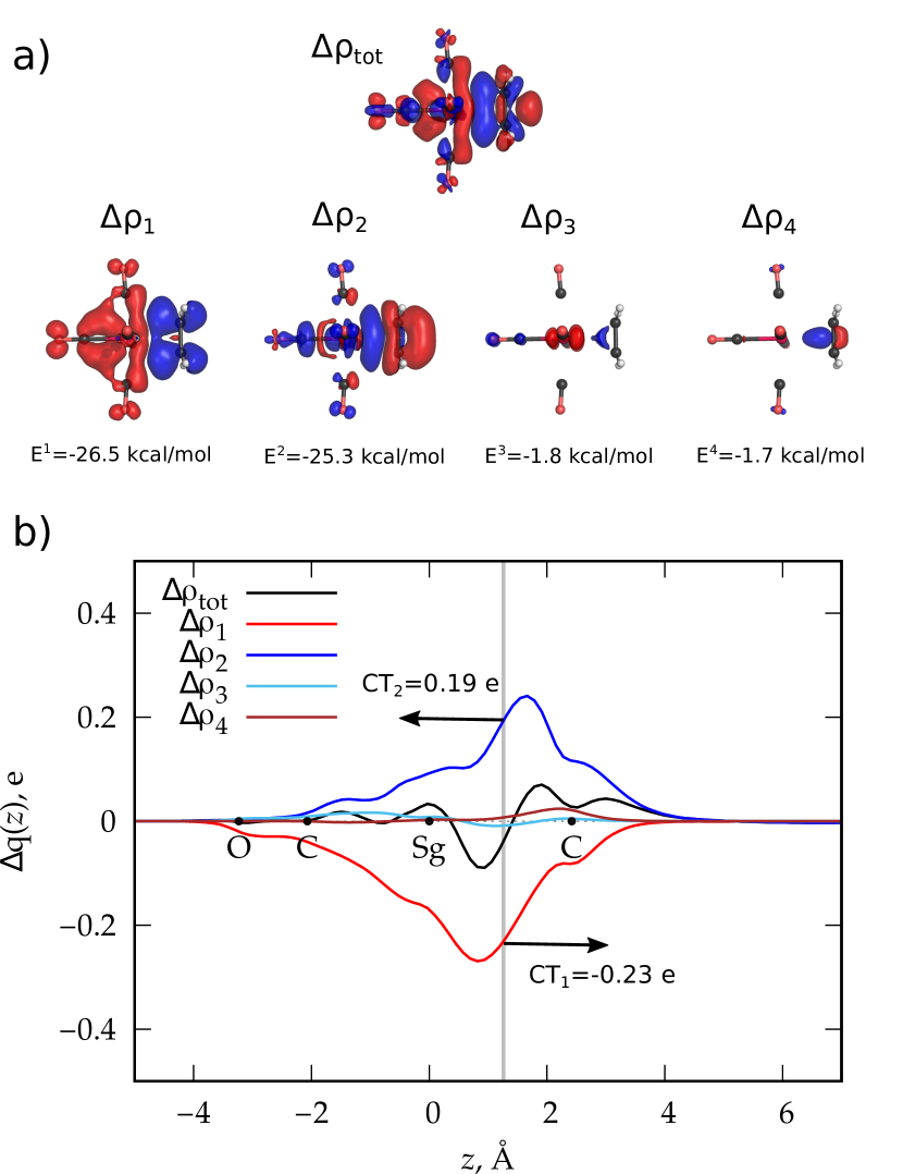
Figure 2: NOCV-CD analysis for the Sg-ethylene bond in the (CO)₅Sg-C₂H₄ complex. a) Contribution to the total deformation density, $\Delta\rho$, of the four most significant NOCV-pairs ($\Delta\rho_{1}$, $\Delta\rho_{2}$, $\Delta\rho_{3}$ and $\Delta\rho_{4}$,).Isodensity surfaces ($\pm 0.0014$ e a.u.^-3) for $\Delta\rho$. Red surfaces identify charge depletion areas, blue surfaces identify charge accumulation areas. b) CD curves. The vertical line marks the boundary between the (CO)₅Sg and the alkene fragment (see text for details). The dots on the axis mark the z coordinate of the atoms.

4 Conclusions

In the present work we have extended the EDA-NOCV method to the relativistic four-component DKS framework. This method allows us to analise a chemical bond in terms of well-defined energy components ($\Delta E_{int}=\Delta E_{elstat}+\Delta E_{Pauli}+\Delta E_{orb}$). It provides a consistent energy/charge splitting scheme, where the different contributions to the orbital relaxation can be easily identified by visualising the associated deformation density and quantified by providing the corresponding stabilization energies. Thanks to this new implementation, the approach can be now applied to the analysis of the chemical bond in molecular systems containing heavy and super-heavy atoms in which the relativistic effects, including spin-orbit coupling, need to be considered at the highest level of accuracy.

This new implementation has been carried out in the framework of the DKS theory, and it has been validated by comparing the results with those obtained using the EDA-NOCV implemented in the ADF package. The benchmark study was successfully performed with different basis sets for selected systems where relativistic effects are not expected to play a significant role. Finally, we have carried out a systematic analysis of the metal-ethylene coordination bond in the group 6-element series (CO)₅TM-C₂H₄, with TM= Cr, Mo, W and Sg, where relativistic effects are likely to play an increasingly important role as one moves down the group. In particular, we have shown that the EDA-NOCV method, in combination with charge displacement analysis, used in the framework of four-component relativistic calculations, is able to identify the donation and back-donation charge fluxes of the Dewar-Chatt-Duncanson bonding model, which is ubiquitous in coordination chemistry. Our analysis shows that the Sg complex has both very similar EDA-NOCV energetic partition and DCD components (donation and back-donation) to those of the W complex and even larger than those of the lighter homologues.

We believe that the methodology presented in this work, together with other advances in the field, [43, 41, 81, 103, 74] may be useful to rationalise the effect of relativity, including spin-orbit coupling, on bonding, reactivity and experimental observations in molecules containing heavy and superheavy elements.

Appendix A Demonstration that the energy difference $E[\rho_{A}+\rho_{B}]-E[\rho_{A}]-E[\rho_{B}]$ is given by the sum of $\Delta E_{elstat}$ and $\Delta E_{XC}^{0}$.

Here we explicitly show that the energy difference between the energy associated with the system obtained using the unmodified electronic densities of the fragments put at their final position in the adduct ($E[\rho_{A}+\rho_{B}]$) and that of the isolated fragments ($E[\rho_{A}]$ and $E[\rho_{B}]$) is given by the sum of the electrostatic interaction ($\Delta E_{elstat}$) plus an exchange-correlation term ($\Delta E^{0}_{XC}$).

We start with the explicit definition of $E[\rho_{A}+\rho_{B}]$ in Eq. A

$$E[\rho_{A}+\rho_{B}] = T_{A+B}-\sum_{a\in\{A,B\}}\int v_{a}(r)(\rho_{A}(r)+\rho_{B}(r))dr+$$

$$+ \frac{1}{2}\int\int\frac{(\rho_{A}(r_{1})+\rho_{B}(r_{1}))(\rho_{A}(r_{2})+\rho_{B}(r_{2}))}{|r_{1}-r_{2}|}dr_{1}dr_{2}+E_{XC}[\rho_{A}+\rho_{B}]+$$

$$+ \sum_{\begin{subarray}{c}i>j\\ {i,j\in\{A,B\}}\end{subarray}}\frac{Z_{i}Z_{j}}{|R_{i}-R_{j}|}$$

where $T_{A+B}$ is the kinetic energy term, $v_{a}(r)$ is the attractive electron-nuclei Coulomb potential for the whole system, the third term is the electronic Coulomb repulsion, $E_{XC}[\rho_{A}+\rho_{B}]$ is the exchange-correlation energy contribution and finally there is the total nuclei-nuclei Coulomb repulsion term. Now, because the orbitals (or spinors) of the two fragments are not allowed to relax in this step of the EDA scheme (see also Fig. 1 in the manuscript), we can easily recognise that the kinetic term $T_{A+B}$ is given by the sum of the kinetic energy of the two separated fragments ($T_{A}$ and $T_{B}$). If we expand Eq. A, gathering togethar those terms that are exclusively associated to one fragment (A or B), and add and subtract the associated exchange-correlation energy terms ($E_{XC}[\rho_{A}$] and $E_{XC}[\rho_{B}$]), we arrive at the following equation

$$\begin{aligned} &\left.\begin{aligned} E[\rho_{A}+\rho_{B}]&=&T_{A}-\sum_{a\in\{A\}}\int v_{a}(r)(\rho_{A}(r))dr+\frac{1}{2}\int\int\frac{\rho_{A}(r_{1})\rho_{A}(r_{2})}{|r_{1}-r_{2}|}dr_{1}dr_{2}+\\ &+&\sum_{\begin{subarray}{c}i>j\\ {i,j\in\{A\}}\end{subarray}}\frac{Z_{i}Z_{j}}{|R_{i}-R_{j}|}+E_{XC}[\rho_{A}]+\\ \end{aligned}\hskip 42.67912pt\right\}\hskip 14.22636pt\text{$E[\rho_{A}]$}\\ &\left.\begin{aligned} \hskip 56.9055pt&+&T_{B}-\sum_{a\in\{B\}}\int v_{a}(r)(\rho_{B}(r))dr+\frac{1}{2}\int\int\frac{\rho_{B}(r_{1})\rho_{A}(r_{2})}{|r_{1}-r_{2}|}dr_{1}dr_{2}+\\ \ &+&\sum_{\begin{subarray}{c}i>j\\ {i,j\in\{B\}}\end{subarray}}\frac{Z_{i}Z_{j}}{|R_{i}-R_{j}|}+E_{XC}[\rho_{B}]-\\ \end{aligned}\hskip 42.67912pt\right\}\hskip 14.22636pt\text{$E[\rho_{B}$]}\\ &\left.\begin{aligned} \hskip 56.9055pt&-&\sum_{a\in\{A\}}\int v_{a}(r)(\rho_{B}(r))dr-\sum_{a\in\{B\}}\int v_{a}(r)(\rho_{A}(r))dr+\sum_{\begin{subarray}{c}i\in\{A\}\\ j\in\{B\}\end{subarray}}\frac{Z_{i}Z_{j}}{|R_{j}-R_{i}|}+\\ &+&\int\int\frac{(\rho_{A}(r_{1})\rho_{B}(r_{2}))}{|r_{1}-r_{2}|}dr_{1}dr_{2}+E_{XC}[\rho_{A}+\rho_{B}]-E_{XC}[\rho_{A}]-E_{XC}[\rho_{B}]\end{aligned}\hskip 2.84544pt\right\}\hskip 11.38092pt\begin{array}[]{c}\Delta E_{elstat}\\ +\\ \Delta E^{0}_{XC}\\ \end{array}\end{aligned}$$

where the first five terms correspond to the definition of the energy of the isolated fragment A ($E[\rho_{A}]$) and the following five sum up to the energy of the isolated fragment B (E[$\rho_{B}$]). Finally, we write the desire energy difference as

$$E[\rho_{A}+\rho_{B}]-E[\rho_{A}]-E[\rho_{B}]=\Delta E_{elstat}+\Delta E^{0}_{XC}$$ (47)

where

$$\Delta E_{elstat}=\sum_{a\in\{A\}}\int v_{a}(r)(\rho_{B}(r))dr-\sum_{a\in\{B\}}\int v_{a}(r)(\rho_{A}(r))dr+\sum_{\begin{subarray}{c}i\in\{A\}\\ j\in\{B\}\end{subarray}}\frac{Z_{i}Z_{j}}{|R_{j}-R_{i}|}+\int\int\frac{(\rho_{A}(r_{1})\rho_{B}(r_{2}))}{|r_{1}-r_{2}|}dr_{1}dr_{2}$$ (48)

defines the electrostatic term of EDA and the term $\Delta E^{0}_{XC}$ identifies an exchange-correlation contribution

$$\Delta E^{0}_{XC} = E_{XC}[\rho_{A}+\rho_{B}]-E_{XC}[\rho_{A}]-E_{XC}[\rho_{B}]$$

which, as pointed out the the main text, is typically included in the Pauli term.

Appendix B Formalism of Transition State (TS) method

The Transition State (TS) formalism was introduced by Slater in the early seventies with the aim to estimate the ionization energy and electronic transitions. [90] Its name may generate a certain confusion for a chemist beacuse it recalls the idea of transtion state theory, however the method is actually a simple scheme to evaluate the energy difference between two states expanding in series their energies around a fictisiuos one (called transition state) settled in between. The method has been extended by Tom Ziegler and A. Rauk to evaluate the bonding energy within the contex of the Hartree-Fock-Slater method[106].

In the following we derive the basis equations, mainly following the original work of Ziegler[106], using only a slighthly different notation (based on one electron density matrix) to be consinstent with the notation used in this work. As mentioned above, the basic idea is to expand in a Taylor series the energy of both the final state ($E[\rho_{f}]$) and the initial state ($E[\rho_{i}]$ respect a common origin, $E[\rho_{T}]$, which is the energy associated with a system with the average density ($\rho_{T}=1/2(\rho_{f}+\rho_{i}$). Analogous to the Taylor expansion of multi-variables function $f(x_{1},...,x_{N})$ around the point $(x^{T}_{1},...,x^{T}_{N})$:

$$f(x_{1},...x_{N})=f(x^{T}_{1},...,x^{T}_{N})+\sum_{i=1}^{N}\left(\frac{\partial f(x_{1},...,x_{N})}{\partial x_{i}}\right)_{(x^{T}_{1},...,x^{T}_{N})}(x_{1}-x^{T}_{1},...,x_{N}-x^{T}_{N})+....$$ (49)

here we expand the Kohn-Sham (or Dirar-Kohn-Sham) energy

$$E_{KS}[\rho]=Tr({\bm{D}h})+\frac{1}{2}Tr({\bm{D}J[D]})+E_{xc}[\rho]$$ (50)

with respect to the one electron density matrix elements $D_{kl}$ where $\rho(r)=\sum_{k,l}D_{kl}\chi^{*}_{k}(r)\chi_{l}(r)$. For the pourpose of the derivation it is usefull to recall that the partial derivative of the Kohn-Sham energy respect the density matrix elements ($D_{ij}$) is given by

$$\frac{\partial E[\rho]}{\partial D_{ij}} = h_{ij}+J_{ij}+\int\underbrace{\frac{\delta E_{xc}[\rho]}{\delta\rho(r)}}_{v^{xc}[\rho](r)}\frac{\partial\rho(r)}{\partial D_{ij}}dr$$ (51)

$$= h_{ij}+J[\rho]_{ij}+V^{XC}[\rho]_{ij}$$ (52)

$$= F[\rho]_{ij}$$ (53)

where $F[\rho]_{ij}$ is the elements of the Kohn-Sham matrix associated with the density, $\rho(r)$. Expanding the energy of both the final state ($E_{KS}[\rho^{f}]$) and the initial state ($E_{KS}[\rho^{i}]$) with respect a common stransition state energy ($E_{KS}[\rho^{T}]$) which corresponds to the energy of a fictisiuos electronic state associated with the everaged density ($\rho^{T}=\frac{1}{2}(\rho^{f}-\rho^{i})$ we have that energies of the two states can be written in terms of the elements of the matrix $\Delta D$ as follows

$$E_{KS}[\rho^{f}] = E_{KS}[\rho^{T}]+\sum_{kl}\left(\frac{\partial E[\rho]}{\partial D_{kl}}\right)_{\rho^{T}}(D^{f}_{kl}-D^{T}_{kl})+$$

$$+ \frac{1}{2}\sum_{klij}\left(\frac{\partial^{2}E[\rho]}{\partial D_{kl}\partial D_{ij}}\right)_{\rho^{T}}(D^{f}_{kl}-D^{T}_{kl})(D^{f}_{ij}-D^{T}_{ij})+O(\Delta D^{3})$$

$$= E_{KS}[\rho^{T}]+\sum_{kl}F[\rho^{T}]_{kl}(\frac{1}{2}\Delta D_{kl})+\frac{1}{2}\left(\frac{\partial^{2}E[\rho]}{\partial D_{kl}\partial D_{ij}}\right)_{\rho^{T}}(\frac{1}{2}\Delta D_{kl})(\frac{1}{2}\Delta D_{ij})+O(\Delta D^{3})$$

$$E_{KS}[\rho^{i}] = E_{KS}[\rho^{T}]+\sum_{kl}\left(\frac{\partial E[\rho]}{\partial D_{kl}}\right)_{\rho^{T}}(D^{i}_{kl}-D^{T}_{kl})+$$

$$+ \frac{1}{2}\sum_{klij}\left(\frac{\partial^{2}E[\rho]}{\partial D_{kl}\partial D_{ij}}\right)_{\rho^{T}}(D^{i}_{kl}-D^{T}_{kl})(D^{i}_{ij}-D^{T}_{ij})+O(\Delta D^{3})$$

$$= E_{KS}[\rho^{T}]+\sum_{kl}F[\rho^{T}]_{kl}(-\frac{1}{2}\Delta D_{kl})+\frac{1}{2}\left(\frac{\partial^{2}E[\rho]}{\partial D_{kl}\partial D_{ij}}\right)_{\rho^{T}}(-\frac{1}{2}\Delta D_{kl})(-\frac{1}{2}\Delta D_{ij})+O(\Delta D^{3})$$

In the above expressions, $D^{T}_{kl}$ are equal to $\frac{1}{2}(D_{kl}^{f}-D_{kl}^{i})$. The second order term in both expansions above cancel out in the energy difference ($E_{KS}[\rho^{f}]-E_{KS}[\rho^{i}]$) and ones obtains an expression which is correct up to the second order and formally linear in $\Delta D$.

$$E_{KS}[\rho^{f}]-E_{KS}[\rho^{i}]=\sum_{kl}F[\rho^{T}]_{kl}(\Delta D_{kl})+O(\Delta D^{3})+..=Tr({\bm{F}}[\rho^{T}]{\bm{\Delta}D}+O(\Delta D^{3})$$ (54)

In their seminal work, Ziegler and Rauk went a step further, deriving even the third order correction showing also this term can be written throught an expression which is formally linear in $\Delta D$. This can be easily showed considereing the third order contribution ($\Delta E(\Delta D^{3})$)

$$\Delta E(\Delta D^{3})=\frac{1}{3!}\frac{1}{4}\sum_{ij,kl,mn}\left(\frac{\partial^{3}E[\rho]}{\partial D_{kl}\partial D_{mn}\partial D_{ij}}\right)_{\rho^{T}}\Delta D_{kl}\Delta D_{mn}\Delta D_{ij}$$ (55)

and using $\frac{\partial E[\rho]}{\partial D_{ij}}=F[\rho]_{ij}$ to write

$$\Delta E(\Delta D^{3})=\frac{1}{3!}\frac{1}{4}\sum_{ij}\left(\sum_{kl,mn}\left(\frac{\partial^{2}F[\rho]_{ij}}{\partial D_{kl}\partial D_{mn}}\right)_{\rho^{T}}\Delta D_{kl}\Delta D_{mn}\right)\Delta D_{ij}$$ (56)

The term in parenthesis in Eq.56 can be evaluated expanding both F$[\rho^{f}]_{ij}$ and F$[\rho^{i}]_{ij}$ in Taylor series around F$[\rho^{T}]_{ij}$

$$F[\rho^{f}]_{ij} = F[\rho^{T}]_{ij}+\sum_{kl}\left(\frac{\partial F[\rho]}{\partial D_{kl}}\right)_{\rho^{T}}(\frac{1}{2}\Delta D_{kl})+\sum_{kl,mn}\frac{1}{2}\left(\frac{\partial^{2}F[\rho]}{\partial D_{kl}\partial D_{mn}}\right)_{\rho^{T}}(\frac{1}{2}\Delta D_{kl})(\frac{1}{2}\Delta D_{mn})$$

$$F[\rho^{i}]_{ij} = F[\rho^{T}]_{ij}+\sum_{kl}\left(\frac{\partial F[\rho]}{\partial D_{kl}}\right)_{\rho^{T}}(-\frac{1}{2}\Delta D_{kl})+\sum_{kl,mn}\frac{1}{2}\left(\frac{\partial^{2}F[\rho]}{\partial D_{kl}\partial D_{mn}}\right)_{\rho^{T}}(-\frac{1}{2}\Delta D_{kl})(-\frac{1}{2}\Delta D_{mn})$$

and by summing term by term we obtain

$$F[\rho^{f}]_{ij}+F[\rho^{i}]_{ij} = 2F[\rho^{T}]_{ij}+\frac{1}{4}\sum_{kl,mn}\left(\frac{\partial^{2}F[\rho]}{\partial D_{kl}\partial D_{mn}}\right)_{\rho^{T}}\Delta D_{kl}\Delta D_{mn}$$ (57)

and rearranging one arrives at Eq. 59

$$\sum_{kl,mn}\left(\frac{\partial^{2}F[\rho]_{ij}}{\partial D_{kl}\partial D_{mn}}\right)_{\rho^{T}}\Delta D_{kl}\Delta D_{mn}=4(F[\rho^{f}]_{ij}+F[\rho^{i}]_{ij}-2F[\rho^{T}]_{ij})$$ (59)

Using this result, the expression originally derived by Ziegler and Rauk and corrected up to the fourth order in $\Delta D$ is given by

$$E_{KS}[\rho^{f}]-E_{KS}[\rho^{i}] = \sum_{ij}F[\rho^{T}]_{ij}(\Delta D_{ij})+\frac{1}{24}\sum_{ij}\sum_{kl,mn}\left(\frac{\partial^{2}F[\rho]_{ij}}{\partial D_{kl}\partial D_{mn}}\right)_{\rho^{T}}\Delta D_{kl}\Delta D_{mn}\Delta D_{ij}$$ (60)

$$= \sum_{ij}F[\rho^{T}]_{ij}(\Delta D_{ij})+\frac{1}{24}\sum_{ij}(4(F[\rho^{f}]_{ij}+F[\rho^{i}]_{ij}-2F[\rho^{T}]_{ij})\Delta D_{ij}$$

$$= \sum_{ij}\left(\frac{2}{3}F[\rho^{T}]_{ij}+\frac{1}{6}F[\rho^{f}]_{ij}+\frac{1}{6}F[\rho^{i}]_{ij}\right)\Delta D_{ij}+O(\Delta D^{5})$$

and is formally linear in $\Delta D$. As already pointed out in the main text, the possibility of write the energy difference ($E_{KS}[\rho^{f}]-E_{KS}[\rho^{i}]$) using formula (see Eq. 54 and Eq. 60), formally linear in $\Delta D_{ij}$, is crucial in order to use the partitioning scheme based on the NOCV method.

Before concluding we mention that the energy difference $E_{KS}[\rho^{f}]-E_{KS}[\rho^{i}]$ can be written with an expression which is formally linear in $\Delta D$ up to an infinity order. van Leeuwen and Baerends showed that it be obtained as a path integral along a path in the space of densities that connects the initial and final densities. A suitable path of the parameter $\alpha$, from $\rho^{i}(\alpha=0)$ to $\rho^{f}(\alpha=1)$ with $\rho(\alpha)$ is a parametric function of $\alpha$ (e. g. $\rho^{f}(\alpha)=\rho^{i}+\alpha\Delta\rho$). More precisely its explicit form is

$$E_{KS}[\rho^{f}]-E_{KS}[\rho^{i}]=\sum_{ij}\Delta D_{ij}\int_{0}^{1}F[\rho(\alpha)]d\alpha$$ (61)

In practice the $\alpha$ integral can be done very accurately by some Gauss numerical integration method over the [0,1] interval but it is rarely necessary to go beyond the mid point or the Simpson rule. Noteworthy, the expression of TS method of Eq. 54 can be obtained using mid point integral approximation over the $\alpha$ parameter in Eq.61 while while its integration using Simpson rule gives exactly the expression derived by Ziegler and Rauk and shown above in Eq. 60.

References

- [1] DIRAC, a relativistic ab initio electronic structure program, Release DIRAC23 (2023), written by R. Bast, A. S. P. Gomes, T. Saue and L. Visscher and H. J. Aa. Jensen, with contributions from I. A. Aucar, V. Bakken, C. Chibueze, J. Creutzberg, K. G. Dyall, S. Dubillard, U. Ekström, E. Eliav, T. Enevoldsen, E. Faßhauer, T. Fleig, O. Fossgaard, L. Halbert, E. D. Hedegård, T. Helgaker, B. Helmich–Paris, J. Henriksson, M. van Horn, M. Iliaš, Ch. R. Jacob, S. Knecht, S. Komorovský, O. Kullie, J. K. Lærdahl, C. V. Larsen, Y. S. Lee, N. H. List, H. S. Nataraj, M. K. Nayak, P. Norman, A. Nyvang, G. Olejniczak, J. Olsen, J. M. H. Olsen, A. Papadopoulos, Y. C. Park, J. K. Pedersen, M. Pernpointner, J. V. Pototschnig, R. di Remigio, M. Repisky, K. Ruud, P. Sałek, B. Schimmelpfennig, B. Senjean, A. Shee, J. Sikkema, A. Sunaga, A. J. Thorvaldsen, J. Thyssen, J. van Stralen, M. L. Vidal, S. Villaume, O. Visser, T. Winther, S. Yamamoto and X. Yuan (available at https://doi.org/10.5281/zenodo.7670749, see also https://www.diracprogram.org).
- Azzopardi et al. [2015] K. M. Azzopardi, G. Bistoni, G. Ciancaleoni, F. Tarantelli, D. Zuccaccia, and L. Belpassi. Quantitative assessment of the carbocation/carbene character of the gold-carbene bond. Dalton Trans., 44:13999–14007, 2015. 10.1039/C5DT02183A. URL http://dx.doi.org/10.1039/C5DT02183A.
- Bader [1990] R. F. Bader. Atoms in molecules: A quantum theory, international series of monographs on chemistry 22. Oxford University Press, Oxford Henkelman G, Arnaldsson A, Jónsson H (2006), 36(3):354–360, 1990.
- Bader et al. [1967a] R. F. W. Bader, W. H. Henneker, and P. E. Cade. Molecular charge distributions and chemical binding. J. Chem. Phys., 46(9):3341–3363, 1967a. http://dx.doi.org/10.1063/1.1841222. URL http://scitation.aip.org/content/aip/journal/jcp/46/9/10.1063/1.1841222.
- Bader et al. [1967b] R. F. W. Bader, I. Keaveny, and P. E. Cade. Molecular charge distributions and chemical binding. II. first-row diatomic hydrides, AH. J. Chem. Phys., 47(9):3381–3402, 1967b. http://dx.doi.org/10.1063/1.1712404. URL http://scitation.aip.org/content/aip/journal/jcp/47/9/10.1063/1.1712404.
- [6] E. J. Baerends, T. Ziegler, A. J. Atkins, J. Autschbach, D. Bashford, O. Baseggio, A. Bérces, F. M. Bickelhaupt, C. Bo, P. M. Boerritger, L. Cavallo, C. Daul, D. P. Chong, D. V. Chulhai, L. Deng, R. M. Dickson, J. M. Dieterich, D. E. Ellis, M. van Faassen, A. Ghysels, A. Giammona, S. J. A. van Gisbergen, A. Goez, A. W. Götz, S. Gusarov, F. E. Harris, P. van den Hoek, Z. Hu, C. R. Jacob, H. Jacobsen, L. Jensen, L. Joubert, J. W. Kaminski, G. van Kessel, C. König, F. Kootstra, A. Kovalenko, M. Krykunov, E. van Lenthe, D. A. McCormack, A. Michalak, M. Mitoraj, S. M. Morton, J. Neugebauer, V. P. Nicu, L. Noodleman, V. P. Osinga, S. Patchkovskii, M. Pavanello, C. A. Peeples, P. H. T. Philipsen, D. Post, C. C. Pye, H. Ramanantoanina, P. Ramos, W. Ravenek, J. I. Rodríguez, P. Ros, R. Rüger, P. R. T. Schipper, D. Schlüns, H. van Schoot, G. Schreckenbach, J. S. Seldenthuis, M. Seth, J. G. Snijders, M. Solà, S. M., M. Swart, D. Swerhone, G. te Velde, V. Tognetti, P. Vernooijs, L. Versluis, L. Visscher, O. Visser, F. Wang, T. A. Wesolowski, E. M. van Wezenbeek, G. Wiesenekker, S. K. Wolff, T. K. Woo, and A. L. Yakovlev. ADF2017, SCM, Theoretical Chemistry, Vrije Universiteit, Amsterdam, The Netherlands. http://www.scm.com.
- Becke [1988] A. D. Becke. Density-functional exchange-energy approximation with correct. Phys. Rev. A, 38:3098–3100, Sep 1988. 10.1103/PhysRevA.38.3098. URL http://link.aps.org/doi/10.1103/PhysRevA.38.3098.
- Becke and Edgecombe [1990] A. D. Becke and K. E. Edgecombe. A simple measure of electron localization in atomic and molecular systems. J. Chem. Phys., 92(9):5397, 1990.
- Belpassi and Storchi [2023] L. Belpassi and L. Storchi. Data set for chemical bond analysis for the entire periodic table: Energy decomposition and natural orbitals for chemical valence in the four- component relativistic framework, June 2023. Data set available at DOI: 10.5281/zenodo.8083284.
- Belpassi et al. [2006] L. Belpassi, F. Tarantelli, A. Sgamellotti, and H. M. Quiney. Electron density fitting for the Coulomb problem in relativistic density-functional theory. J. Chem. Phys., 124(12):124104, 2006. http://dx.doi.org/10.1063/1.2179420. URL http://scitation.aip.org/content/aip/journal/jcp/124/12/10.1063/1.2179420.
- Belpassi et al. [2008] L. Belpassi, I. Infante, F. Tarantelli, and L. Visscher. The chemical bond between Au(I) and the noble gases. comparative study of NgAuF and NgAu+ (Ng = Ar, Kr, Xe) by density functional and coupled cluster methods. J. Am. Chem. Soc., 130(3):1048–1060, 2008. 10.1021/ja0772647. URL http://pubs.acs.org/doi/abs/10.1021/ja0772647.
- Belpassi et al. [2011] L. Belpassi, L. Storchi, H. M. Quiney, and F. Tarantelli. Recent advances and perspectives in four-component Dirac-Kohn-Sham calculations. Phys. Chem. Chem. Phys., 13:12368–12394, 2011. 10.1039/C1CP20569B. URL http://dx.doi.org/10.1039/C1CP20569B.
- Belpassi et al. [2020] L. Belpassi, M. De Santis, H. M. Quiney, F. Tarantelli, and L. Storchi. BERTHA: Implementation of a four-component Dirac–Kohn–Sham relativistic framework. The Journal of Chemical Physics, 152(16):164118, apr 2020. ISSN 0021-9606. 10.1063/5.0002831. URL http://aip.scitation.org/doi/10.1063/5.0002831.
- Bickelhaupt and Baerends [2000] F. M. Bickelhaupt and E. J. Baerends. Kohn-Sham Density Functional Theory: Predicting and Understanding Chemistry, pages 1–86. John Wiley & Sons, Ltd, 2000. ISBN 9780470125922. https://doi.org/10.1002/9780470125922.ch1. URL https://onlinelibrary.wiley.com/doi/abs/10.1002/9780470125922.ch1.
- Bistoni et al. [2013] G. Bistoni, L. Belpassi, and F. Tarantelli. Disentanglement of donation and back-donation effects on experimental observables: A case study of gold-ethyne complexes. Angew. Chem. Int. Ed., 52(44):11599–11602, 2013. ISSN 1521-3773. 10.1002/anie.201305505. URL http://dx.doi.org/10.1002/anie.201305505.
- Bistoni et al. [2015] G. Bistoni, S. Rampino, F. Tarantelli, and L. Belpassi. Charge-displacement analysis via natural orbitals for chemical valence: Charge transfer effects in coordination chemistry. J. Chem. Phys., 142(8):084112, 2015. http://dx.doi.org/10.1063/1.4908537. URL http://scitation.aip.org/content/aip/journal/jcp/142/8/10.1063/1.4908537.
- Bistoni et al. [2016a] G. Bistoni, P. Belanzoni, L. Belpassi, and F. Tarantelli. activation of alkynes in homogeneous and heterogeneous gold catalysis. J. Phys. Chem. A, pages 5239–5246, 2016a.
- Bistoni et al. [2016b] G. Bistoni, L. Belpassi, and F. Tarantelli. Advances in charge displacement analysis. J. Chem. Theory Comput., 12(3):1236–1244, 2016b. 10.1021/acs.jctc.5b01166. URL http://dx.doi.org/10.1021/acs.jctc.5b01166.
- Bistoni et al. [2016c] G. Bistoni, S. Rampino, N. Scafuri, G. Ciancaleoni, D. Zuccaccia, L. Belpassi, and F. Tarantelli. How back-donation quantitatively controls the co stretching response in classical and non-classical metal carbonyl complexes. Chem. Sci., 7:1174–1184, 2016c. 10.1039/C5SC02971F. URL http://dx.doi.org/10.1039/C5SC02971F.
- Cappelletti et al. [2012] D. Cappelletti, E. Ronca, L. Belpassi, F. Tarantelli, and F. Pirani. Revealing charge-transfer effects in gas-phase water chemistry. Accounts Chem. Res., 45(9):1571–1580, 2012. 10.1021/ar3000635. URL http://dx.doi.org/10.1021/ar3000635.
- Champion et al. [2011] J. Champion, M. Seydou, A. Sabatie-Gogova, E. Renault, G. Montavon, and N. Galland. Assessment of an effective quasirelativistic methodology designed to study astatine chemistry in aqueous solution. Phys. Chem. Chem. Phys., 13:14984–14992, 2011. 10.1039/C1CP20512A. URL http://dx.doi.org/10.1039/C1CP20512A.
- Chandra et al. [2001] R. Chandra, L. Dagum, D. Kohr, R. Menon, D. Maydan, and J. McDonald. Parallel programming in OpenMP. Morgan kaufmann, 2001.
- Chatt and Duncanson [1953] J. Chatt and L. A. Duncanson. Olefin co-ordination compounds. part iii. infra-red spectra and structure: Attempted preparation of acetylene complexes. J. Chem. Soc., pages 2939–2942, 1953. 10.1039/JR9530002939.
- Ciancaleoni et al. [2015] G. Ciancaleoni, L. Biasiolo, G. Bistoni, A. Macchioni, F. Tarantelli, D. Zuccaccia, and L. Belpassi. Selectively measuring back-donation in gold (i) complexes by nmr spectroscopy. Chem. Eur. J., 21(6):2467–2473, 2015.
- Coppens and Hall [1982] P. Coppens and M. B. Hall, editors. Electron distributions and the chemical bond. Plenum Press, New York, USA, 1982.
- Coulson [1955] C. A. Coulson. The contributions of wave mechanics to chemistry (resumed). J. Chem. Soc., page 2069, 1955.
- Dapprich and Frenking [1995] S. Dapprich and G. Frenking. Investigation of donor-acceptor interactions: A charge decomposition analysis using fragment molecular orbitals. J. Phys. Chem., 99(23):9352, 1995.
- De Santis et al. [2018] M. De Santis, S. Rampino, H. M. Quiney, L. Belpassi, and L. Storchi. Charge-displacement analysis via natural orbitals for chemical valence in the four-component relativistic framework. Journal of chemical theory and computation, 14(3):1286–1296, 2018.
- De Santis et al. [2019] M. De Santis, S. Rampino, L. Storchi, L. Belpassi, and F. Tarantelli. The chemical bond and s–d hybridization in coinage metal (i) cyanides. Inorganic Chemistry, 58(17):11716–11729, 2019.
- De Santis et al. [2020] M. De Santis, L. Storchi, L. Belpassi, H. M. Quiney, and F. Tarantelli. Pyberthart: A relativistic real-time four-component tddft implementation using prototyping techniques based on python. J. Chem. Theory Comput., 16(4):2410–2429, 2020. 10.1021/acs.jctc.0c00053.
- Demissie et al. [2016] T. B. Demissie, B. D. Garabato, K. Ruud, and P. M. Kozlowski. Mercury methylation by cobalt corrinoids: Relativistic effects dictate the reaction mechanism. Angew. Chem. Int. Ed., 55(38):11503–11506, 2016. ISSN 1521-3773. 10.1002/anie.201606001. URL http://dx.doi.org/10.1002/anie.201606001.
- Dewar [1951] M. J. S. Dewar. A review of complex theory. Bull. Soc. Chim. Fr., 18:C71–79, 1951.
- Dunning [1989] T. H. Dunning. Gaussian basis sets for use in correlated molecular calculations. I. The atoms boron through neon and hydrogen. The Journal of Chemical Physics, 90(2):1007–1023, jan 1989. ISSN 0021-9606. 10.1063/1.456153. URL http://aip.scitation.org/doi/10.1063/1.456153.
- Dunning et al. [2023] T. H. Dunning, M. S. Gordon, and S. S. Xantheas. The nature of the chemical bond. The Journal of Chemical Physics, 158(13):130401, 2023. 10.1063/5.0148500. URL https://doi.org/10.1063/5.0148500.
- Dyall [2002] K. G. Dyall. Relativistic and nonrelativistic finite nucleus optimized triple-zeta basis sets for the 4, 5 and 6 elements. Theor. Chem. Acc., 108(6):335–340, 2002. ISSN 1432-881X. 10.1007/s00214-002-0388-0. URL http://dx.doi.org/10.1007/s00214-002-0388-0. Basis sets are available from the Dirac web site, http://dirac.chem.sdu.dk.
- Dyall [2004] K. G. Dyall. Relativistic double-zeta, triple-zeta, and quadruple-zeta basis sets for the 5 elements Hf-Hg. Theor. Chem. Acc., 112(5-6):403–409, 2004. ISSN 1432-881X. 10.1007/s00214-004-0607-y. URL http://dx.doi.org/10.1007/s00214-004-0607-y. Basis sets are available from the Dirac web site, http://dirac.chem.sdu.dk.
- Dyall [2006] K. G. Dyall. Relativistic Quadruple-Zeta and Revised Triple-Zeta and Double-Zeta Basis Sets for the 4p, 5p, and 6p Elements. Theor. Chem. Acc., 115(5):441–447, 2006. ISSN 1432-881X. 10.1007/s00214-006-0126-0. URL http://dx.doi.org/10.1007/s00214-006-0126-0.
- Dyall [2009] K. G. Dyall. Relativistic double-zeta, triple-zeta, and quadruple-zeta basis sets for the 4s, 5s, 6s, and 7s elements. J. Phys. Chem. A, 113(45):12638–12644, 2009. 10.1021/jp905057q.
- Dyall [2023] K. G. Dyall. Dyall dz, tz, and qz basis sets for relativistic electronic structure calculations, 2023. aae2z and aae3z basis set available at DOI: 10.5281/zenodo.7574628.
- Dyall and Gomes [2010] K. G. Dyall and A. S. Gomes. Revised relativistic basis sets for the 5 elements Hf-Hg. Theor. Chem. Acc., 125(1-2):97–100, 2010. ISSN 1432-881X. 10.1007/s00214-009-0717-7. URL http://dx.doi.org/10.1007/s00214-009-0717-7. Basis sets are available from the Dirac web site, http://dirac.chem.sdu.dk.
- Eickerling et al. [2007] G. Eickerling, R. Mastalerz, V. Herz, W. Scherer, H.-J. Himmel, and M. Reiher. Relativistic effects on the topology of the electron density. J. Chem. Theory Comput., 3(6):2182–2197, 2007. URL http://dx.doi.org/10.1021/ct7001573.
- Esterhuysen and Frenking [2004] C. Esterhuysen and G. Frenking. The nature of the chemical bond revisited. an energy partitioning analysis of diatomic molecules e2 (e=n-bi, f-i), co and bf. Theor. Chem. Acc., 111(2-6):381, 2004.
- Faegri and Saue [2001] K. Faegri and T. Saue. Diatomic molecules between very heavy elements of group 13 and group 17: A study of relativistic effects on bonding. J. Chem. Phys., 115(6):2456–2464, 2001. 10.1063/1.1385366.
- Frenking [2001] G. Frenking. Understanding the nature of the bonding in transition metal complexes: from dewar’s molecular orbital model to an energy partitioning analysis of the metal–ligand bond. J. Organom. Chem., 635(1):9–23, 2001.
- Frenking and Fröhlich [2000] G. Frenking and N. Fröhlich. The nature of the bonding in transition-metal compounds. Chem. Rev., 100(2):717, 2000.
- Fuse et al. [2017] M. Fuse, I. Rimoldi, E. Cesarotti, S. Rampino, and V. Barone. On the relation between carbonyl stretching frequencies and the donor power of chelating diphosphines in nickel dicarbonyl complexes. Phys. Chem. Chem. Phys., 19:9028–9038, 2017. 10.1039/C7CP00982H. URL http://dx.doi.org/10.1039/C7CP00982H.
- Gaggioli et al. [2016] C. A. Gaggioli, L. Belpassi, F. Tarantelli, D. Zuccaccia, J. N. Harvey, and P. Belanzoni. Dioxygen insertion into the gold(i)-hydride bond: Spin orbit coupling effects in the spotlight for oxidative addition. Chem. Sci., 7:7034–7039, 2016. 10.1039/C6SC02161A. URL http://dx.doi.org/10.1039/C6SC02161A.
- Gaggioli et al. [2017] C. A. Gaggioli, G. Bistoni, G. Ciancaleoni, F. Tarantelli, L. Belpassi, and P. Belanzoni. Modulating the bonding properties of n-heterocyclic carbenes (nhcs): A systematic charge-displacement analysis. Chem. Eur. J., 23(31):7558–7569, 2017. ISSN 1521-3765. 10.1002/chem.201700638. URL http://dx.doi.org/10.1002/chem.201700638.
- Gaggioli et al. [2018] C. A. Gaggioli, L. Belpassi, F. Tarantelli, J. N. Harvey, and P. Belanzoni. Frontispiece: Spin-forbidden reactions: Adiabatic transition states using spin–orbit coupled density functional theory. Chemistry – A European Journal, 24(20), 2018. https://doi.org/10.1002/chem.201882061. URL https://chemistry-europe.onlinelibrary.wiley.com/doi/abs/10.1002/chem.201882061.
- Gorin and Toste [2007] D. J. Gorin and F. D. Toste. Relativistic effects in homogeneous gold catalysis. Nature, 446(7134):395, 2007.
- Grant [2007] I. P. Grant. Relativistic quantum theory of atoms and molecules: theory and computation, volume 40. Springer Science & Business Media, 2007.
- Grant and Quiney [2000] I. P. Grant and H. M. Quiney. Rayleigh-Ritz approximation of the Dirac operator in atomic and molecular physics. Phys. Rev. A, 62:022508, 2000. 10.1103/PhysRevA.62.022508. URL http://link.aps.org/doi/10.1103/PhysRevA.62.022508.
- Ilias and Pershina [2017] M. Ilias and V. Pershina. Hexacarbonyls of mo, w, and sg: Metal–co bonding revisited. Inorganic Chemistry, 56(3):1638–1645, 2017. 10.1021/acs.inorgchem.6b02759. URL https://doi.org/10.1021/acs.inorgchem.6b02759. PMID: 28103024.
- Jacob and Reiher [2012] C. R. Jacob and M. Reiher. Spin in density-functional theory. Int. J. Quantum Chem., 112(23):3661–3684, 2012. ISSN 1097-461X. 10.1002/qua.24309. URL http://dx.doi.org/10.1002/qua.24309.
- Jacobsen and Ziegler [1994] H. Jacobsen and T. Ziegler. Nonclassical double bonds in ethylene analogs: Influence of pauli repulsion on trans bending and -bond strength. a density functional study. J. Am. Chem. Soc., 116(9):3667–3679, 1994.
- Jeziorski et al. [1994] B. Jeziorski, R. Moszynski, and K. Szalewicz. Molecular charge distributions and chemical binding. J. Am. Chem. Soc., 94(7):1887, 1994.
- Kitaura and Morokuma [1976] K. Kitaura and K. Morokuma. A new energy decomposition scheme for molecular interactions within the hartree-fock approximation. Int. J. Quantum Chem., 10(2):325, 1976.
- [58] A. M. Köster, D. R. Salahub, and et al. demon2k, version 4, the demon developers. deMon2k, Version 4, The deMon developers. Cinvestav, Mexico City (2016).
- L. Storchi [2023] L. B. L. Storchi, M. De Santis, 2023. REL 1.0.0 URL: https://github.com/BERTHA-4c-DKS/pybertha/releases/tag/XXXXXX within the PyBertha project: https://github.com/BERTHA-4c-DKS/pybertha/ (Accessed: June written by: L. Storchi, M. De Santis, L. Belpassi.
- Li et al. [1995] J. Li, G. Schreckenbach, and T. Ziegler. Relativistic effects on metal-ligand bond strengths in -complexes: Quasi-relativistic density functional study of m (ph3) 2x2 (m= ni, pd, pt; x2= o2, c2h2, c2h4) and m (co) 4 (c2h4)(m= fe, ru, os). Inorg. Chem., 34(12):3245–3252, 1995.
- Marchione et al. [2017] D. Marchione, M. A. Izquierdo, G. Bistoni, R. W. Havenith, A. Macchioni, D. Zuccaccia, F. Tarantelli, and L. Belpassi. 13c nmr spectroscopy of n-heterocyclic carbenes can selectively probe donation in gold (i) complexes. Chem. Eur. J., 23(11):2722–2728, 2017.
- Mariusz P. Mitoraj [2008] T. Z. Mariusz P. Mitoraj, Artur Michalak. A combined charge and energy decomposition scheme for bond analysis. J. Chem. Theory Comput., 4(4):962–975, 2008. 10.1021/ct800503d.
- Michalak et al. [2008] A. Michalak, M. Mitoraj, and T. Ziegler. Bond orbitals from chemical valence theory. J. Phys. Chem. A, 112(9):1933–1939, 2008.
- Mitoraj and Michalak [2007] M. Mitoraj and A. Michalak. Donor-acceptor properties of ligands from the natural orbitals for chemical valence. Organometallics, 26(26):6576–6580, 2007.
- Mitoraj et al. [2009] M. P. Mitoraj, A. Michalak, and T. Ziegler. A combined charge and energy decomposition scheme for bond analysis. J. Chem. Theory Comput., 5(4):962–975, 2009. 10.1021/ct800503d.
- Mitoraj M. [2007] M. A. Mitoraj M. Natural orbitals for chemical valence as descriptors of chemical bonding in transition metal complexes. J. Mol. Model., 13:347–355, 2007.
- Mo et al. [2000] Y. Mo, J. Gao, and S. D. Peyerimhoff. Energy decomposition analysis of intermolecular interactions using a block-localized wave function approach. J. Chem. Phys., 112(13):5530, 2000.
- Mülliken [1955] R. S. Mülliken. Electronic population analysis on lcaomo molecular wave functions. J. Chem. Phys., 23(10):1833, 1955.
- Nalewajski and Mrozek [1994] R. F. Nalewajski and J. Mrozek. Modified valence indices from the two-particle density matrix. Int. J. Quantum Chem., 51(4):187–200, 1994. ISSN 1097-461X. 10.1002/qua.560510403. URL http://dx.doi.org/10.1002/qua.560510403.
- Nalewajski et al. [1993] R. F. Nalewajski, A. M. Köster, and K. Jug. Chemical valence from the two-particle density matrix. Theor. Chem. Acc., 85(6):463–484, 1993. ISSN 0040-5744. 10.1007/BF01112985. URL http://dx.doi.org/10.1007/BF01112985.
- Nalewajski et al. [1997] R. F. Nalewajski, J. Mrozek, and A. Michalak. Two-electron valence indices from the kohn-sham orbitals. Int. J. Quantum Chem., 61(3):589–601, 1997. ISSN 1097-461X. 10.1002/(SICI)1097-461X(1997)61:3¡589::AID-QUA28¿3.0.CO;2-2. URL http://dx.doi.org/10.1002/(SICI)1097-461X(1997)61:3<589::AID-QUA28>3.0.CO;2-2.
- Nechaev et al. [2004] M. S. Nechaev, V. M. Rayón, and G. Frenking. …. The Journal of Physical Chemistry A, 108(15):3134–3142, 2004. 10.1021/jp031185+.
- Perdew [1986] J. P. Perdew. Density-functional approximation for the correlation energy of the inhomogeneous electron gas. Phys. Rev. B, 33:8822–8824, Jun 1986. 10.1103/PhysRevB.33.8822. URL https://link.aps.org/doi/10.1103/PhysRevB.33.8822.
- Pilmè et al. [2014] J. Pilmè, E. Renault, F. Bassal, M. Amaouch, G. Montavon, and N. Galland. Qtaim analysis in the context of quasirelativistic quantum calculations. J. Chem. Theory Comput., 10(11):4830–4841, 2014. 10.1021/ct500762n.
- Pyykko [1988] P. Pyykko. Relativistic effects in structural chemistry. Chem. Rev., 88(3):563–594, 1988.
- Quiney and Belanzoni [2002] H. M. Quiney and P. Belanzoni. Relativistic density functional theory using Gaussian basis sets. J. Chem. Phys., 117(12):5550–5563, 2002. http://dx.doi.org/10.1063/1.1502245. URL http://scitation.aip.org/content/aip/journal/jcp/117/12/10.1063/1.1502245.
- Radoń [2008] M. Radoń. On the properties of natural orbitals for chemical valence. Theor. Chem. Acc., 120(4-6):337–339, 2008. ISSN 1432-881X. 10.1007/s00214-008-0428-5. URL http://dx.doi.org/10.1007/s00214-008-0428-5.
- Rampino et al. [2014] S. Rampino, L. Belpassi, F. Tarantelli, and L. Storchi. Full parallel implementation of an all-electron four-component Dirac-kohn-Sham program. J. Chem. Theory Comput., 10(9):3766–3776, 2014. 10.1021/ct500498m. URL http://dx.doi.org/10.1021/ct500498m.
- Ricciarelli et al. [2020] D. Ricciarelli, L. Belpassi, J. N. Harvey, and P. Belanzoni. Spin-forbidden reactivity of transition metal oxo species: Exploring the potential energy surfaces. Chemistry – A European Journal, 26(14):3080–3089, 2020. https://doi.org/10.1002/chem.201904314. URL https://chemistry-europe.onlinelibrary.wiley.com/doi/abs/10.1002/chem.201904314.
- Rossi et al. [2020] E. Rossi, M. De Santis, D. Sorbelli, L. Storchi, L. Belpassi, and P. Belanzoni. Spin–orbit coupling is the key to unraveling intriguing features of the halogen bond involving astatine. Physical Chemistry Chemical Physics, 22(4):1897–1910, 2020.
- Sablon et al. [2010] N. Sablon, R. Mastalerz, F. De Proft, P. Geerlings, and M. Reiher. Relativistic effects on the fukui function. Theor. Chem. Acc., 127(3):195–202, Oct 2010. ISSN 1432-2234. 10.1007/s00214-009-0722-x. URL https://doi.org/10.1007/s00214-009-0722-x.
- Saue et al. [2020] T. Saue, R. Bast, A. S. P. Gomes, H. J. A. Jensen, L. Visscher, I. A. Aucar, R. Di Remigio, K. G. Dyall, E. Eliav, E. Fasshauer, T. Fleig, L. Halbert, E. D. Hedegård, B. Helmich-Paris, M. Iliaš, C. R. Jacob, S. Knecht, J. K. Laerdahl, M. L. Vidal, M. K. Nayak, M. Olejniczak, J. M. H. Olsen, M. Pernpointner, B. Senjean, A. Shee, A. Sunaga, and J. N. P. van Stralen. The dirac code for relativistic molecular calculations. The Journal of Chemical Physics, 152(20):204104, 2020. 10.1063/5.0004844. URL https://doi.org/10.1063/5.0004844.
- Saunders [1983] V. Saunders. Molecular integrals for gaussian type functions. In Methods in Computational Molecular Physics, pages 1–36. Springer, 1983.
- Schuchardt et al. [2007] K. L. Schuchardt, B. T. Didier, T. Elsethagen, L. Sun, V. Gurumoorthi, J. Chase, J. Li, and T. L. Windus. Basis set exchange: A community database for computational sciences. J. Chem. Information and Modeling, 47(3):1045–1052, 2007. 10.1021/ci600510j. URL http://dx.doi.org/10.1021/ci600510j.
- Schwarz [2003] H. Schwarz. Relativistic effects in gas-phase ion chemistry: An experimentalist’s view. Angew. Chem. Int. Ed., 42(37):4442–4454, 2003.
- Schwarz et al. [1985] W. H. E. Schwarz, P. Valtazanos, and K. Ruedenberg. Electron difference densities and chemical bonding. Theor. Chim. Acta, 68(6):471–506, Dec 1985. ISSN 1432-2234. 10.1007/BF00527670. URL https://doi.org/10.1007/BF00527670.
- Schwerdtfeger [2014] P. Schwerdtfeger. Relativity and Chemical Bonding, pages 383–404. Wiley-VCH Verlag GmbH & Co. KGaA, 2014. ISBN 9783527664696. 10.1002/9783527664696.ch11. URL http://dx.doi.org/10.1002/9783527664696.ch11.
- Schwerdtfeger et al. [1992] P. Schwerdtfeger, G. A. Heath, M. Dolg, and M. A. Bennett. Low valencies and periodic trends in heavy element chemistry. a theoretical study of relativistic effects and electron correlation effects in group 13 and period 6 hydrides and halides. J. Am. Chem. Soc., 114(19):7518–7527, 1992.
- Senjean et al. [2021] B. Senjean, S. Sen, M. Repisky, G. Knizia, and L. Visscher. Generalization of intrinsic orbitals to kramers-paired quaternion spinors, molecular fragments, and valence virtual spinors. Journal of Chemical Theory and Computation, 17(3):1337–1354, 2021. 10.1021/acs.jctc.0c00964. URL https://doi.org/10.1021/acs.jctc.0c00964. PMID: 33555866.
- Slater [1972] J. C. Slater. Statistical exchange-correlation in the self-consistent field. volume 6 of Advances in Quantum Chemistry, pages 1–92. Academic Press, 1972. https://doi.org/10.1016/S0065-3276(08)60541-9. URL https://www.sciencedirect.com/science/article/pii/S0065327608605419.
- Sorbelli et al. [2020] D. Sorbelli, M. De Santis, P. Belanzoni, and L. Belpassi. Spectroscopic/bond property relationship in group 11 dihydrides via relativistic four-component methods. The Journal of Physical Chemistry A, 124(50):10565–10579, 2020. 10.1021/acs.jpca.0c09043. URL https://doi.org/10.1021/acs.jpca.0c09043. PMID: 33327724.
- Sorbelli et al. [2021] D. Sorbelli, L. Belpassi, and P. Belanzoni. Reactivity of a gold-aluminyl complex with carbon dioxide: A nucleophilic gold? Journal of the American Chemical Society, 143(36):14433–14437, 2021. 10.1021/jacs.1c06728. URL https://doi.org/10.1021/jacs.1c06728. PMID: 34472349.
- Sorbelli et al. [2022a] D. Sorbelli, L. Belpassi, and P. Belanzoni. Mechanistic study of alkyne insertion into cu–al and au–al bonds: A paradigm shift for coinage metal chemistry. Inorganic Chemistry, 61(51):21095–21106, 2022a. 10.1021/acs.inorgchem.2c03713. URL https://doi.org/10.1021/acs.inorgchem.2c03713. PMID: 36493466.
- Sorbelli et al. [2022b] D. Sorbelli, L. Belpassi, and P. Belanzoni. What singles out aluminyl anions? a comparative computational study of the carbon dioxide insertion reaction in gold-aluminyl, -gallyl, and -indyl complexes. Inorganic Chemistry, 61(3):1704–1716, 2022b. 10.1021/acs.inorgchem.1c03579. URL https://doi.org/10.1021/acs.inorgchem.1c03579. PMID: 34986633.
- Sorbelli et al. [2022c] D. Sorbelli, E. Rossi, R. W. Havenith, J. E. Klein, L. Belpassi, and P. Belanzoni. Gold-aluminyl and gold-diarylboryl complexes: Bonding and reactivity with carbon dioxide. Inorganic Chemistry, 61(19):7327–7337, 2022c. 10.1021/acs.inorgchem.2c00174. URL https://doi.org/10.1021/acs.inorgchem.2c00174. PMID: 35512414.
- Sorbelli et al. [2023a] D. Sorbelli, L. Belpassi, and P. Belanzoni. Radical-like reactivity for dihydrogen activation by coinage metal–aluminyl complexes: computational evidence inspired by experimental main group chemistry. Chem. Sci., 14:889–896, 2023a. 10.1039/D2SC05815D. URL http://dx.doi.org/10.1039/D2SC05815D.
- Sorbelli et al. [2023b] D. Sorbelli, L. Belpassi, and P. Belanzoni. Widening the landscape of small molecule activation with gold-aluminyl complexes: A systematic study of e-h (e=o, n) bonds, so2 and n2o activation. Chemistry – A European Journal, 29(21):e202203584, 2023b. https://doi.org/10.1002/chem.202203584. URL https://chemistry-europe.onlinelibrary.wiley.com/doi/abs/10.1002/chem.202203584.
- Storchi et al. [2010] L. Storchi, L. Belpassi, F. Tarantelli, A. Sgamellotti, and H. M. Quiney. An efficient parallel all-electron four-component Dirac-Kohn-Sham program using a distributed matrix approach. J. Chem. Theory Comput., 6(2):384–394, 2010. 10.1021/ct900539m. URL http://pubs.acs.org/doi/abs/10.1021/ct900539m.
- Storchi et al. [2013] L. Storchi, S. Rampino, L. Belpassi, F. Tarantelli, and H. M. Quiney. Efficient parallel all-electron four-component Dirac-Kohn-Sham program using a distributed matrix approach II. J. Chem. Theory Comput., 9(12):5356–5364, 2013. 10.1021/ct400752s. URL http://pubs.acs.org/doi/abs/10.1021/ct400752s.
- Storchi et al. [2019] L. Storchi, M. De Santis, and L. Belpassi. {BERTHA} and PyBERTHA: State of the Art for Full Four-Component Dirac-Kohn-Sham Calculations. In I. T. Foster, G. R. Joubert, L. Kucera, W. E. Nagel, and F. J. Peters, editors, Parallel Computing: Technology Trends, Proceedings of the International Conference on Parallel Computing, {PARCO} 2019, Prague, Czech Republic, September 10-13, 2019, volume 36 of Advances in Parallel Computing, pages 354–363. {IOS} Press, 2019. 10.3233/APC200060. URL 10.3233/APC200060.
- te Velde et al. [2001] G. te Velde, F. M. Bickelhaupt, E. J. Baerends, C. Fonseca Guerra, S. J. A. van Gisbergen, J. G. Snijders, and T. Ziegler. Chemistry with ADF. J. Comput. Chem., 22(9):931–967, jul 2001. ISSN 0192-8651. 10.1002/jcc.1056. URL https://onlinelibrary.wiley.com/doi/10.1002/jcc.1056.
- Visscher [1997] L. Visscher. Theor. Chem. Acc., 98:68, 1997.
- Zeng et al. [2011] T. Zeng, D. G. Fedorov, M. W. Schmidt, and M. Klobukowski. Effects of spin-orbit coupling on covalent bonding and the jahn-teller effect are revealed with the natural language of spinors. J. Chem. Theory Comput., 7(9):2864–2875, 2011. 10.1021/ct200457q.
- Zhao et al. [2018] L. Zhao, M. von Hopffgarten, D. M. Andrada, and G. Frenking. Energy decomposition analysis. WIREs Computational Molecular Science, 8(3):e1345, 2018. https://doi.org/10.1002/wcms.1345. URL https://wires.onlinelibrary.wiley.com/doi/abs/10.1002/wcms.1345.
- Zhao et al. [2019] L. Zhao, S. Pan, N. Holzmann, P. Schwerdtfeger, and G. Frenking. Chemical bonding and bonding models of main-group compounds. Chemical Reviews, 119(14):8781–8845, 2019. 10.1021/acs.chemrev.8b00722. URL https://doi.org/10.1021/acs.chemrev.8b00722. PMID: 31251603.
- Ziegler and Rauk [1977] T. Ziegler and A. Rauk. On the calculation of bonding energies by the hartree fock slater method. Theor. Chem. Acc., 46(1):1, 1977.