Mean Field Theory in Deep Metric Learning

Abstract

In this paper, we explore the application of mean field theory, a technique from statistical physics, to deep metric learning and address the high training complexity commonly associated with conventional metric learning loss functions. By adapting mean field theory for deep metric learning, we develop an approach to design classification-based loss functions from pair-based ones, which can be considered complementary to the proxy-based approach. Applying the mean field theory to two pair-based loss functions, we derive two new loss functions, MeanFieldContrastive and MeanFieldClassWiseMultiSimilarity losses, with reduced training complexity. We extensively evaluate these derived loss functions on three image-retrieval datasets and demonstrate that our loss functions outperform baseline methods in two out of the three datasets.

1 Introduction

Deep metric learning has emerged as a powerful technique for learning meaningful data representations in a variety of machine learning applications, such as image retrieval [1], face recognition [2], and person re-idenfication [3]. The primary goal of deep metric learning is to provide an order to the embedding space by bringing similar instances closer and pushing dissimilar ones further apart. Typically, this is achieved by optimizing a loss function that utilizes appropriate interactions based on the distance between data points. However, conventional metric learning loss functions often suffer from high training complexity scaling polynomially with the size of the training data. This challenge makes optimization of these loss functions difficult in large-scale applications and necessitates the development of sampling and mining strategies to find informative pairs

The concept of order also plays a crucial role in statistical physics, which studies the emergent behaviors of interacting many-body systems. These many-body systems exhibit various ordered phases of matter, such as solid state, magnetism, superfluidity, and superconductivity, which cannot be predicted from their individual constituents [4]. While the interactions between the constituents are essential for hosting such nontrivial behaviors, they also make analyzing the systems challenging, analogous to the issue in deep metric learning.

Mean field theory [5] is a powerful approach for handling the challenge associated with interacting many-body systems and provides an insightful framework for understanding their emergent behaviors. This theory introduces a mean field that represents the average behavior of constituent particles. The mean field is also known as the order parameter, as its value helps distinguish the ordered phases. The mean field theory approximates their interactions as interactions with the mean field and significantly reduces the complexity of many-body systems.

In this paper, we leverage mean field theory from statistical physics to tackle the complexity associated with deep metric learning. We develop the mean field theory for applications to loss functions in deep metric learning and find that mean field theory is better suited for losses without anchor concepts, as opposed to the proxy-based method introduced in Ref. [6]. In this sense, it can serve as a complementary approach to the proxy-based method for designing classification-based loss functions from pair-based ones. Furthermore, we apply the mean field theory to two pair-based loss functions and propose two new loss functions with reduced training complexity. We evaluate the proposed mean field loss functions using a benchmark protocol proposed in Ref. [7], which allows us a fair comparison with other baseline loss functions, and also using the traditional protocol utilized in Ref. [6, 8]. The evaluation results indicate that our mean field losses surpass other methods in two out of three image-retrieval datasets in the former protocol. Moreover, the latter evaluation protocol demonstrates that our losses not only exhibit performance improvements in three out of four image-retrieval datasets but also converge more rapidly compared to ProxyAnchor loss [8].

The main contributions of this paper are three-fold: (1) the introduction of the mean field theory from statistical physics as a tool to reduce the training complexity of pair-based loss functions based on an analogy between magnetism and deep metric learning; (2) the derivation of MeanFieldContrastive and MeanFieldClassWiseMultiSimilarity losses by application of the mean field theory to two pair-based loss functions; (3) the demonstration that the derived loss functions are competitive with existing baseline losses in several datasets.

2 Related work

2.1 Pair-based loss functions

Pair-based loss functions, a representative category of deep metric learning losses, leverage pairwise or triplet relationships among data points. Contrastive loss [9] is an early example of this type, which utilizes positive and negative pairs of data and learns embeddings to place the positive pairs close and negative ones apart. Triplet loss [10] is an extension of Contrastive loss, which exploits triplets of positive, negative, and anchor data, and places an anchor embedding closer to a positive than a negative. These losses are further extended to incorporate interactions among pairs in mini-batches to improve performance and convergence speed [11, 12, 13, 14]. For instance, MultiSimilarity loss [14] takes into account multiple inter-pair relationships within a mini-batch, enabling more efficient learning of the embedding space.

However, a major drawback of the pair-based losses is their sensitivity to the choice of positive and negative pairs, which is caused by the polynomial growth of the number of pairs and triplets with respect to the number of training data [2]. This usually requires sophisticated sampling and mining strategies for informative pairs to improve performance and mitigate slow convergence [2, 15, 3, 16, 17, 18, 14]. In this paper, we pursue an alternative approach to reduce training complexity rather than investigate these strategies. We accomplish this by leveraging the mean field theory, a concept from statistical physics.

2.2 Classfication-based loss functions

Classification-based loss functions utilize weight matrices and learn embeddings by optimizing a classification objective. Unlike pair-based losses, these losses do not face the complexity issue because they are computed in the same manner as a typical classification task.

A representative example is NormalizedSoftmax loss [19, 20], which is obtained by the cross-entropy loss function with an L2-normalized weight matrix. Its extensions include SphereFace [21], ArcFace [22], and CosFace [23, 24] losses obtained by modifying distance metrics and introducing margins. The losses with proxies such as ProxyTriplet and ProxyNCA losses also belong to this category [6]. Such proxy losses can be derived from corresponding pair-based losses by substituting positive and negative data points with learnable embeddings called proxies while retaining anchors. ProxyAnchor loss [8] further considers interactions among samples in a mini-batch and shows promising performance in popular public datasets, surpassing other classification-based and pair-based loss functions. These losses have been extended to incorporate refined structures among data, such as graphs [25], hierarchies [26], and others [27, 28, 29].

In this paper, we develop the mean field theory as a technique to derive a classification-based loss from a pair-based one, addressing the challenges of the latter. Although our approach is similar to the proxy-based method, it naturally adapts to pair-based losses without anchors, which have remained unexplored by the proxy-based method.

3 Proposed approach

In this section, we investigate the mean field theory and its application to deep metric learning. We first review the mean field theory for a ferromagnet in statistical mechanics by following standard statistical mechanics textbooks (e.g., see Ref. [30]). Next, based on the analogy between the ferromagnet and deep metric learning, we apply the mean field approximation to the Contrastive loss and a variant of the MultiSimilarity loss and derive classification-type loss functions with reduced training complexity.

3.1 Mean field theory for magnets

Magnetism is one of the representative phenomena in statistical physics that show a phase transition between ordered and disordered phases. A ferromagnet is composed of a large number of microscopic magnetic spins and shows a macroscopic magnetization when a macroscopic number of the magnetic spins are aligned in the same direction.

To explain the mean field theory for a ferromagnet, we shall consider an infinite-range model whose Hamiltonian (or energy) takes the following form [30]:

$$\begin{split}\mathcal{H}=-\frac{J}{2}\sum^{N}_{i,j=1}S^{T}_{i}\cdot S_{j},\end{split}$$ (1)

with the total number of spins $N\in\mathbb{N}$ and the exchange interaction $J>0$. Here, $S_{i}\in S^{2}$ represents the $i$-th constituent magnetic spin. Eq.(1) indicates that a state where spins point in the same direction is preferred energetically.

According to statistical mechanics, a probabilistic distribution of the spin configuration at temperature $T$ follows the Gibbs distribution:

$$\begin{split}P(\{S_{i}\}_{i})=\frac{\mathrm{e}^{-\mathcal{H}/T}}{Z},\quad Z=\int\prod_{i}d^{2}S_{i}\mathrm{e}^{-\mathcal{H}/T},\end{split}$$ (2)

and macroscopic properties of this system can be computed from the normalization factor $Z$. However, since the spins are interacting with each other, it is not easy to compute $Z$ both analytically and numerically.

To address this difficulty, we introduce the mean field theory. The central idea of the theory is to approximate the Hamiltonian (1) such that each spin interacts with an average field generated by the rest of the spins, rather than with other spins directly, thereby ignoring their fluctuations. More concretely, it means that we expand $\mathcal{H}$ with respect to fluctuations $\{(S_{i}-M)\}_{i}$ using the identity, $S_{i}=M+(S_{i}-M)$ and ignore the second-order terms of the expansion. This operation results in

$$\begin{split}\mathcal{H}\simeq\mathcal{H}_{\mathrm{MFT}}=\frac{JN^{2}}{2}M^{T}\cdot M-JNM^{T}\cdot\sum^{N}_{i=1}S_{i}.\end{split}$$ (3)

Since $\mathcal{H}_{\mathrm{MFT}}$ does not include interaction terms between spins, one can readily compute any information from the Gibbs distribution for this Hamiltonian as follows:

$$\begin{split}P_{\mathrm{MFT}}(\{S_{i}\}_{i})=\frac{\mathrm{e}^{-\mathcal{H}_{\mathrm{MFT}}/T}}{Z_{\mathrm{MFT}}},\quad Z_{\mathrm{MFT}}=\int\prod_{i}d^{2}S_{i}\mathrm{e}^{-\mathcal{H}_{\mathrm{MFT}}/T}.\end{split}$$ (4)

The value of the mean field $M$ must be determined to minimize $-\log Z_{\mathrm{MFT}}$. This condition is justified because we can show that it is equivalent to

$$\begin{split}M=\frac{1}{N}\sum_{i}\mathbb{E}[S_{i}]\end{split}$$ (5)

by differentiating $-\log Z_{\mathrm{MFT}}$ with respect to the mean field. Here, we take the expectation value over the Gibbs distribution $P_{\mathrm{MFT}}$ in Eq. (5). Since the mean field approximation is based on the expansion with respect to the fluctuations around the mean field, Eq. (5) ensures the consistency of expansion.

Overall, the mean field theory is a powerful tool that allows us to describe and analyze complex systems by approximating the interactions between individual constituents with an average field generated by the rest of the system. To draw a parallel between the above discussion and deep metric learning, let us consider the $T\rightarrow 0$ limit. In this limit, the original problem of computing $Z$ becomes one of finding a spin configuration that minimizes $\mathcal{H}$. This is analogous to a machine learning problem that seeks optimal parameters to minimize a loss function. Then, the mean field approximation reduces the problem to one of minimizing $\mathcal{H}_{\mathrm{MFT}}$ with respect to both the spins and mean field. Therefore, this observation indicates that applications of mean field theory to deep metric learning problems introduce mean fields as parameters learned to minimize their loss functions.

3.2 Mean field contrastive loss

To study how the mean field theory works for loss functions in deep metric learning, let us begin by applying the mean field theory to Contrastive loss for the sake of simplicity and then proceed to discuss the mean field theory for a more complicated loss function.

In the following sections, we denote training data by $\mathcal{D}=\{x_{i},y_{i}\}^{|\mathcal{D}|}_{i=1}$ composed of input data $x_{i}$ and its class label $y_{i}\in\mathcal{C}=\{1,\cdots,|\mathcal{C}|\}$. We also denote a set of data in class $c\in\mathcal{C}$ as $\mathcal{D}_{c}$. We extract features from the input data using a machine learning model $F_{\theta}$, whose learnable parameters are represented by $\theta$. This model embeds the input into a manifold $\mathcal{M}$, such as $\mathbb{R}^{d}$ or $S^{d}$, with $d\in\mathbb{N}$. We also define the distance between two embeddings, $F,F^{\prime}\in\mathcal{M}$, as $d(F,F^{\prime})\geq 0$. For instance, the distance can be given by the cosine distance for $\mathcal{M}=S^{d}$, taking the form $d(F,F^{\prime})=1-F^{T}\cdot F^{\prime}/(||F||_{2}||F^{\prime}||_{2})$, or by the Euclidean distance for $\mathcal{M}=\mathbb{R}^{d}$.

Contrastive loss is one of the primitive examples in deep metric learning, which is defined as

$$\begin{split}\mathcal{L}_{\mathrm{Cont.}}=&\frac{1}{2|\mathcal{C}|}\sum_{c\in\mathcal{C}}\frac{1}{|\mathcal{D}_{c}|^{2}}\sum_{i,j\in\mathcal{D}_{c}}\Big{[}d(F_{\theta}(x_{i}),F_{\theta}(x_{j}))-m_{\mathrm{P}}\Big{]}_{+}\\ &+\frac{1}{2|\mathcal{C}|}\sum_{c\neq c^{\prime}}\frac{1}{|\mathcal{D}_{c}||\mathcal{D}_{c^{\prime}}|}\sum_{i\in\mathcal{D}_{c},j\in\mathcal{D}_{c^{\prime}}}\Big{[}m_{\mathrm{N}}-d(F_{\theta}(x_{i}),F_{\theta}(x_{j})\Big{]}_{+},\end{split}$$ (6)

with $[x]_{+}=\max(x,0)$. Here, $m_{\mathrm{P}}$ ($m_{\mathrm{N}}$) is a hyperparamter that controls distances between positive (negative) instances. Note that Eq. (6) reduces to the Hamiltonian (1) when $|\mathcal{C}|=1$ and $m_{\mathrm{P}}<0$, and it requires the $\mathcal{O}(|\mathcal{D}|^{2})$ training complexity as it is parallel to the situation in Sec. 3.1.

This analogy encourages us to apply the mean field theory in order to obtain a simpler loss function. Since we have multiple classes here, we shall introduce mean fields $\{M_{c}\}_{c\in\mathcal{C}}$ and expand $\mathcal{L}_{\mathrm{Cont.}}$ with respect to fluctuations around them. Note that, in contrast to the single-class case, we must impose the following conditions to constrain relative distance among the mean fields:

$$\begin{split}\Big{[}m_{\mathrm{N}}-d(M_{c},M_{c^{\prime}})\Big{]}_{+}=0\quad\Bigl{(}c\neq c^{\prime}\Bigr{)}.\end{split}$$ (7)

This condition means that we should explore configurations of the mean fields which minimize $\mathcal{L}_{\mathrm{Cont.}}$ at the zeroth order of expansions around the mean fields. In practice, we take into account these constraints softly.

In the expansion around the mean fields, we ignore all cross-product terms of the fluctuations keeping any others so that we reduce the complexity while taking into account the higher-order terms of self-interactions. By summing over the remaining terms, we obtain MeanFieldContrastive (MFCont.) loss, which takes the following form:

$$\begin{split}\mathcal{L}_{\mathrm{MFCont.}}=&\frac{1}{|\mathcal{C}|}\sum_{c\in\mathcal{C}}\frac{1}{|\mathcal{D}_{c}|}\sum_{i\in\mathcal{D}_{c}}\Big{(}\Big{[}d(F_{\theta}(x_{i}),M_{c})-m_{\mathrm{P}}\Big{]}_{+}+\sum_{c^{\prime}(\neq c)}\Big{[}m_{\mathrm{N}}-d(F_{\theta}(x_{i}),M_{c})\Big{]}_{+}\Big{)}\\ &+\frac{\lambda_{\mathrm{MF}}}{|\mathcal{C}|}\sum_{c\neq c^{\prime}}\Big{[}m_{\mathrm{N}}-d(M_{c},M_{c^{\prime}})\Big{]}^{2}_{+},\end{split}$$ (8)

where we impose the constraints (7) softly by $\lambda_{\mathrm{MF}}>0$. Note that resummation here naïvely produces unstable terms, $\{-[m_{\mathrm{N}}-(d(M_{c},M_{c^{\prime}})]_{+}\}_{c,c^{\prime}}$, but they vanish, thanks to the constraints (7). We emphasize that we must minimize $\mathcal{L}_{\mathrm{MFCont.}}$ by optimizing both $M_{c}$ and $\theta$, and we can readily show that the optimal mean fields satisfy $M_{c}=\sum_{i\in\mathcal{D}_{c}}F_{\theta}(x_{i})/|\mathcal{D}_{c}|$ at the first order of fluctuations.

3.3 Mean field class-wise multisimilarity loss

Lastly, we consider the mean field approximation of a loss function which incorporates interactions within a mini-batch similar to MultiSimilarity [14] and ProxyAnchor [8] losses. However, the mean field approximation relies on expansions around mean fields, and thus, a loss function symmetric with respect to $x_{i}$ and $x_{j}$ (i.e., without anchors) would be more desirable for our purpose. Since most loss functions do not exhibit such a symmetric property, we propose the following loss function that satisfies these requirements:

$$\begin{split}\mathcal{L}_{\mathrm{CWMS}}=&\frac{1}{\alpha|\mathcal{C}|}\sum_{c\in\mathcal{C}}\log\left[1+\frac{\sum_{i,j\in\mathcal{D}_{c}}e^{\alpha(d(F_{\theta}(x_{i}),F_{\theta}(x_{j}))-\delta)}}{2|\mathcal{D}_{c}|^{2}}\right]\\ &+\frac{1}{2\beta|\mathcal{C}|}\sum_{c\neq c^{\prime}}\log\left[1+\frac{\sum_{i\in\mathcal{D}_{c},j\in\mathcal{D}_{c^{\prime}}}e^{-\beta(d(F_{\theta}(x_{i}),F_{\theta}(x_{j}))-\delta)}}{|\mathcal{D}_{c}||\mathcal{D}_{c^{\prime}}|}\right],\end{split}$$ (9)

with hyperparameters $\alpha$, $\beta$, and $\delta$. Since Eq. (9) takes a similar form to MultiSimilarity loss [14] but incorporates interactions among negative samples in a class-wise manner, we refer to it as ClassWiseMultiSimilarity (CWMS) loss.

Next, we derive the mean field counterpart of this loss function. Here, the logits in the first and second terms take forms similar to the positive and negative interactions found in Contrastive loss (6). Repeating the discussion in Sec. 3.2, we derive MeanFieldClassWiseMultiSimilarity (MFCWMS) loss:

$$\begin{split}\mathcal{L}_{\mathrm{MFCWMS}}=&\frac{1}{\alpha|\mathcal{C}|}\sum_{c\in\mathcal{C}}\log\left[1+\frac{\sum_{i\in\mathcal{D}_{c}}e^{\alpha(d(F_{\theta}(x_{i}),M_{c})-\delta)}}{|\mathcal{D}_{c}|}\right]\\ +&\frac{1}{2\beta|\mathcal{C}|}\sum_{c\neq c^{\prime}}\log\left[1+\frac{\sum_{i\in\mathcal{D}_{c}}e^{-\beta(d(F_{\theta}(x_{i}),M_{c^{\prime}})-\delta)}}{|\mathcal{D}_{c}|}+\frac{\sum_{j\in\mathcal{D}_{c^{\prime}}}e^{-\beta(d(M_{c},F_{\theta}(x_{j}))-\delta)}}{|\mathcal{D}_{c^{\prime}}|}\right]\\ +&\frac{\lambda_{\mathrm{MF}}}{|\mathcal{C}|}\sum_{c\neq c^{\prime}}\left(\log\left[1+e^{-\beta(d(M_{c},M_{c^{\prime}})-\delta)}\right]\right)^{2},\end{split}$$ (10)

where we also introduce the soft constraint for the mean fields to ignore unstable terms produced in the resummation. Compared to MeanFieldContrastive loss, this loss function incorporates interactions of positive samples as well as those of negative ones in a class-wise manner like ProxyAnchor loss.

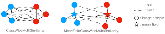
Figure 1: Schematic illustration of interactions in CWMS (left) and MFCWMS (right) losses. Each color indicates a class to which an embedding and a mean field belong.

4 Experiments

Let us see the effectiveness of the proposed mean field losses by evaluating their image-retrieval performance in several public datasets. We employ the recently proposed benchmarking scheme [7] as well as the traditional one used in Refs. [6, 8]. We compare our mean field losses and existing loss functions, such as MultiSimilarity and ProxyAnchor losses. We also explore the effect of hyperparameters on their evaluation metrics. In our experiment, we use precision at $1$ (P@1), R-precision (RP), and mean average precision at R (MAP@R) as evaluation metrics. In particular, we focus on MAP@R because it reflects the correctness of the ranking for retrievals and is a suitable metric to evaluate the quality of the embedding space [7]. Note that we implement our experiments in PyTorch [31] and utilize the PyTorch Metric Learning library [32] to implement baseline models.

4.1 Datasets

In our experiments, we utilize four publicly available image-retrieval datasets, CUB-200-2011 (CUB) [33], Cars-196 (Cars) [34], Stanford Online Products (SOP) [12], and In-Shop [35]. CUB comprises $11{,}788$ images of birds categorized into $200$ classes, while the Cars dataset consists of $16{,}185$ images of $196$ car classes. In CUB, the first $100$ classes ($5{,}864$ images) are used for the training dataset, and the remaining $100$ classes ($5{,}924$ images) are allocated for the test dataset. Similarly, Cars was split into $8{,}054$ training images ($98$ classes) and $8{,}131$ test images ($98$ classes). The SOP dataset contains $22{,}634$ classes with $120{,}053$ product images. The initial $11{,}318$ classes with $59{,}551$ images are used for training, and the remaining $11{,}316$ classes with $60{,}502$ images are allocated for testing. Lastly, the InShop dataset features $52{,}712$ images of $7{,}982$ fashion products, with $25{,}882$ images from $3{,}997$ classes used for training and $26{,}830$ images from $3{,}985$ classes allocated for testing, which are further divided into query ($14{,}218$ images) and gallery ($12{,}612$ images) subsets.

4.2 Implementation details

As a backbone embedding model $F_{\theta}(x)$, we employ the inception network with batch normalization (BN-Inception) [36], which is pretrained for the classification task on the ImageNet dataset [37]. We reduce the embedding dimensions by inserting a fully-connected layer with ReLU activation functions in the first scheme and replacing its last linear layer with that of desired dimensions in the second scheme. In both cases, we apply random resized cropping and random horizontal flipping to all inputs during training and only center cropping during evaluation.

In the modern benchmarking protocol, we perform $50$ iterations of Bayesian optimization for hyperparameters in loss functions including the learning rate for proxies and mean fields for a fair comparison. We split a dataset into train–valid (the first half classes) and test datasets (the remainings). The train–valid set was further divided into four partitions in a class disjoint manner, and we performed four-fold cross-validation based on the leave-one-out method in each iteration. In each cross-validation step, we train a model with embedding dimensions set to $128$ and batch size set to $32$ until MAP@R for the validation data converges. The Bayesian optimization aims to maximize the average of the four validation metrics. Note that we sample images so that each mini-batch is composed of $32$ classes ($8$ classes) and $1$ image ($4$ images) per class for classification-based (pair-based) losses, and we utilize the RMSprop optimizer with learning rate $10^{-6}$ for the embedding model. In the test stage, we perform cross-validation again with the best hyperparameters, resulting in four embedding models. Using these models, we evaluate performance on the test dataset in the following two different ways: mean of the metrics computed from the $128$-dimensional ($128$D) embeddings (separated) and those from $512$D embeddings made of the four $128$D ones (concatenated). We repeat this observation $10$ times and report their average values with $95\%$ intervals. We carry out the experiments on a single NVIDIA V100 GPU.

In contrast, in the traditional evaluation protocol, we use the predefined train–test splits described in Sec. 4.1 and train a model for up to $60$ epochs with embedding dimensions $512$ and batch size $128$, setting the patience for early stopping to $5$ to accelerate the experiments. In this case, we use AdamW optimizer [38] with the learning rate $10^{-4}$ for the embedding model, setting the learning rate for proxies to $10^{-2}$ and that for mean fields to $2\times 10^{-1}$. The hyperparameters for ProxyAnchor loss are fixed to $(\alpha,\delta)=(32,10^{-1})$, while we set $(m_{\mathrm{P}},m_{\mathrm{N}},\lambda_{\mathrm{MF}})=(0.02,0.3,0)$ for MFCont. loss and $(\alpha,\beta,\delta,\lambda_{\mathrm{MF}})=(0.01,80,0.8,0)$ for MFCWMS loss in default. We chose these default parameters according to the results of the Bayesian optimization and the discussion in Sec. 4.4. We repeat the above procedure $10$ times and report the averages of the metrics computed from the test embedding with the best MAP@R with $95$% confidence intervals. The experiments on the CUB and Cars datasets are carried out on a single NVIDIA V100 GPU, while those on the SOP and InShop datasets are performed on a single NVIDIA A100 GPU.

4.3 Benchmark results

Based on the first protocol, we study the performance of our loss functions on three datasets; CUB, Cars, and SOP. We compare our loss functions with existing ones, such as Contrastive, MultiSimilarity, ArcFace, CosFace, ProxyNCA, and ProxyAnchor losses. The experimental results are summarized in Table 1 (see the supplement for complete results). First, the mean field losses show better performance than their original pair-based losses in most cases, indicating that applying mean field theory not only reduces training complexity but also results in better embeddings. Furthermore, the mean field losses consistently outperform other baseline methods in both separate and concatenated MAP@R for the CUB and SOP datasets. However, in Cars, ProxyAnchor and CWMS losses show better performance than the mean field losses, which might imply the importance of interactions within batch samples in this dataset.

Table 1: MAP@R obtained from the modern protocol [7] in CUB-200-2011, Cars-196, and Stanford Online Products. We carry out test runs $10$ times and present the averaged metrics along with their confidence intervals. The best result within each block is highlighted in bold, while the overall best results for all losses are underlined. ProxyAnchor loss failed to converge in the SOP dataset in our settings. See the supplement for complete results.

	CUB		Cars		SOP
Loss	$128$D	$512$D	$128$D	$512$D	$128$D	$512$D
ArcFace	${21.5\pm 0.1}$	${26.4\pm 0.2}$	${18.3\pm 0.1}$	$\mathbf{27.6\pm 0.1}$	${41.5\pm 0.2}$	$\mathbf{47.4\pm 0.2}$
CosFace	${21.2\pm 0.2}$	$\mathbf{26.5\pm 0.3}$	${18.5\pm 0.1}$	${27.0\pm 0.3}$	${41.0\pm 0.2}$	${46.8\pm 0.2}$
MS	${21.0\pm 0.2}$	${26.2\pm 0.2}$	${18.7\pm 0.3}$	${27.2\pm 0.4}$	${41.9\pm 0.2}$	${46.7\pm 0.2}$
MS+Miner	${20.8\pm 0.2}$	${25.9\pm 0.2}$	${18.5\pm 0.2}$	${26.9\pm 0.4}$	${41.9\pm 0.3}$	${46.6\pm 0.3}$
ProxyNCA	${18.8\pm 0.2}$	${23.8\pm 0.2}$	${17.4\pm 0.1}$	${26.8\pm 0.2}$	$\mathbf{42.7\pm 0.1}$	${46.7\pm 0.1}$
ProxyAnch.	$\mathbf{21.7\pm 0.2}$	$\mathbf{26.5\pm 0.2}$	$\underline{\mathbf{19.4\pm 0.2}}$	${26.8\pm 0.3}$	$\mathrm{-}$	$\mathrm{-}$
Cont.	${21.0\pm 0.1}$	${26.4\pm 0.2}$	${17.0\pm 0.3}$	${24.9\pm 0.5}$	${41.1\pm 0.2}$	${45.3\pm 0.2}$
MFCont.	$\mathbf{22.0\pm 0.1}$	$\underline{\mathbf{27.2\pm 0.1}}$	$\mathbf{18.1\pm 0.1}$	$\mathbf{27.4\pm 0.2}$	$\mathbf{43.6\pm 0.4}$	$\mathbf{47.0\pm 0.2}$
CWMS	${21.5\pm 0.3}$	${26.9\pm 0.3}$	$\mathbf{19.3\pm 0.3}$	$\underline{\mathbf{27.8\pm 0.3}}$	${41.5\pm 0.2}$	${45.1\pm 0.2}$
MFCWMS	$\underline{\mathbf{22.1\pm 0.1}}$	$\mathbf{27.0\pm 0.1}$	${18.9\pm 0.2}$	${27.0\pm 0.3}$	$\underline{\mathbf{44.6\pm 0.2}}$	$\underline{\mathbf{48.3\pm 0.2}}$

We also test the performance in the four datasets described in Sec. 4.1 following the traditional protocol. As shown in Tables 3 and 3, our mean field losses outperform ProxyAnchor loss in MAP@R except for the Cars dataset, which is consistent with the first experiment. The improvement in accuracy is evident in the larger datasets. Besides, MFCont. and MFCWMS losses converge faster than ProxyAnchor loss in all the datasets. See also the supplement for plots of learning curves.

Table 2: MAP@R values and epochs with the best accuracies obtained using the traditional protocol [6, 8] on the CUB and Cars datasets. The best result in each block is highlighted in bold.

	CUB		Cars
Loss	MAP@R ($\uparrow$)	Epoch ($\downarrow$)	MAP@R ($\uparrow$)	Epoch ($\downarrow$)
ProxyAnch.	${25.1\pm 0.2}$	${11.5\pm 1.4}$	$\mathbf{26.3\pm 0.2}$	${23.6\pm 1.8}$
MFCont.	$\mathbf{25.3\pm 0.3}$	$\mathbf{4.4\pm 0.4}$	${24.7\pm 0.2}$	${10.1\pm 0.5}$
MFCWMS	$\mathbf{25.3\pm 0.3}$	${4.7\pm 0.6}$	${24.0\pm 0.2}$	$\mathbf{8.5\pm 0.8}$

Table 3: MAP@R values and epochs with the best accuracies obtained using the traditional protocol [6, 8] on the SOP and InShop datasets. The best result in each block is highlighted in bold.

	SOP		InShop
Loss	MAP@R ($\uparrow$)	Epoch ($\downarrow$)	MAP@R ($\uparrow$)	Epoch ($\downarrow$)
ProxyAnch.	${51.5\pm 0.3}$	${40.5\pm 6.5}$	${65.5\pm 0.1}$	${31.3\pm 7.2}$
MFCont.	$\mathbf{52.9\pm 0.1}$	${25.1\pm 1.4}$	$\mathbf{67.7\pm 0.2}$	${24.1\pm 2.7}$
MFCWMS	${52.7\pm 0.0}$	$\mathbf{23.0\pm 1.3}$	${67.5\pm 0.4}$	$\mathbf{20.6\pm 2.1}$

4.4 Impact of hyperparameters

Embedding dimensions.

Since embedding dimensions are crucial hyperparameters controlling the performance of image retrieval, we investigate their effect on the accuracy (MAP@R). On the CUB dataset, we run the traditional experiments for ProxyAnchor, MFCont., and MFCWMS losses by varying the embedding dimensions from $32$ to $1024$. The results are shown in Fig. 3. We find that our mean field losses monotonically increase their performance and consistently show better performance compared to ProxyAnchor loss. Notably, the performance improvement is significantly larger in the cases of $64$, $128$, and $256$ dimensions, suggesting that our proposed methods potentially offer efficient embeddings in relatively small dimensions.

Figure 2: MAP@R versus embedding dimensions in CUB, comparing ProxyAnchor, MFCont., and MFCWMS losses.

Figure 3: MAP@R against $\beta$ and $\delta$ of MFCWMS loss in the CUB dataset.

Batch size.

We also investigate how batch size affects the accuracy of our models. We compare the test performance of MFCWMS loss by changing the batch size between $30$ and $180$ for CUB and Cars (Table 5) and $30$ and $300$ for SOP and InShop (Table 5). The accuracy metric basically improves as the batch size increases. The improvement mostly saturates around $150$ and $180$ for the smaller datasets and around $150$ and $300$ for SOP. In the InShop dataset, we observe that the accuracy drops around batch size $150$ with a relatively large variance, but this can be consistent with ProxyAnchor loss since it also decreases its accuracy around this batch size (see the supplement).

Table 4: Impact of batch size to MAP@R for MFCWMS loss in CUB and Cars. Batch size CUB Cars ${30}$ ${23.3\pm 0.3}$ ${22.0\pm 0.3}$ ${60}$ ${24.4\pm 0.1}$ ${23.2\pm 0.3}$ ${90}$ ${25.1\pm 0.1}$ ${23.6\pm 0.4}$ ${120}$ ${25.3\pm 0.2}$ ${23.9\pm 0.2}$ ${150}$ $\mathbf{25.4\pm 0.3}$ $\mathbf{24.2\pm 0.3}$ ${180}$ $\mathbf{25.4\pm 0.2}$ $\mathbf{24.2\pm 0.2}$

Table 5: Impact of batch size to MAP@R for MFCWMS loss in SOP and InShop. Batch size SOP InShop ${30}$ ${51.1\pm 0.1}$ ${67.4\pm 0.2}$ ${60}$ ${52.0\pm 0.1}$ ${67.6\pm 0.2}$ ${90}$ ${52.4\pm 0.1}$ ${67.6\pm 0.2}$ ${120}$ ${52.7\pm 0.1}$ $\mathbf{67.8\pm 0.2}$ ${150}$ ${52.8\pm 0.1}$ ${67.0\pm 0.6}$ ${300}$ $\mathbf{53.0\pm 0.3}$ ${67.0\pm 0.4}$

$\beta$ and $\delta$ of MFCWMS.

We also explore the effect of $\beta$ and $\delta$ of MFCWMS loss in the CUB dataset. We varied $\beta$ from $50$ to $90$ and $\delta$ from $0.6$ to $1$, fixing $(\alpha,\lambda_{\mathrm{MF}})$ to $(0.01,0)$ and computed the MAP@R for the test data. The results are summarized in Fig. 3. Fig. 3 ensures the competitive performance of the MFCWMS loss is stable against a choice of the hyperparameters. We observe that the preferred $\beta$ gradually decreases as the margin parameter $\delta$ decreases.

Mean field regularization.

Finally, we study the impact of the regularization term in Eq. (10). We investigate the test performance of MFCont. and MFCWMS losses in the CUB dataset varying the scale of the regularization coefficient, which is summarized in Table 6. The results indicate that the regularization does not offer a statistically significant difference in performance. This is because the constraint (7) should be satisfied naturally when the main parts of the mean field losses are minimized. Thus, we conclude that the constraints in MFCont. and MFCWMS losses are significant theoretically, but less relevant in practice.

Table 6: MAP@R against the regularization coefficient $\lambda_{\mathrm{MF}}$ in Eq. (10) in the CUB dataset.

$\lambda_{\mathrm{MF}}$	0	0.01	0.1	1	10	100
MFCont.	${25.2\pm 0.3}$	${25.2\pm 0.3}$	$\mathbf{25.3\pm 0.3}$	${25.2\pm 0.2}$	${25.2\pm 0.3}$	${25.0\pm 0.3}$
MFCWMS	$\mathbf{25.3\pm 0.2}$	$\mathbf{25.3\pm 0.3}$	$\mathbf{25.3\pm 0.3}$	$\mathbf{25.3\pm 0.3}$	${25.2\pm 0.3}$	${25.1\pm 0.3}$

5 Conclusion

In this paper, we explored applications of the mean field theory in statistical physics to address the challenges in training complexity associated with conventional metric learning loss functions. The mean field theory replaces interactions among data points with interactions with mean fields, approximating pair-based losses by classification-based ones. While the mean field theory shares a similar philosophy with the proxy-based method [6], it relies on expansions with respect to fluctuations around the mean fields and is suitable for applications to pair-based losses without anchors.

Based on the analogy between deep metric learning and magnets, we applied the mean field theory to Contrastive loss and ClassWiseMultiSimilarity loss, a variant of MultiSimilarity loss [14] without anchors, and derived MeanFieldContrastive and MeanFieldClassWiseMultiSimilarity losses. We extensively evaluated the proposed loss functions and compared them with the existing baseline methods using both modern and traditional benchmark protocols. The evaluation results demonstrate that the proposed loss functions outperform the baselines in the CUB-200-2011 (CUB) and Stanford Online Products (SOP) datasets in the former protocol, and in the CUB, SOP, and InShop datasets in the latter. These findings highlight the potential of mean field theory as a powerful tool for simplifying and improving deep metric learning performance in various machine learning applications.

Limitations

Despite the promising results demonstrated by the proposed loss functions, this work has the following limitations that should be acknowledged:

• Theoretical guarantees: Since our approach is based on the idea of physics, our discussion primarily focuses on its conceptual description and practical utility. Its mathematical aspects, including rigorous proof and theoretical analysis of convergence properties, have not been explored.

• Multi-label settings: The current study focuses on single-label classification tasks, where each image belongs to only one class. The applicability and performance of the proposed loss functions in multi-label settings, where an image can belong to multiple classes, have not been investigated.

These limitations should be addressed in future work.

 

Supplementary Material

 

Appendix A Additional experimental results

In this section, we present the experimental results that cannot be shown in the main paper due to the page limit.

MLRC results.

Tables 9 – 9 show the complete results of Table 1 in the main paper, which are obtained the modern benchmark protocol proposed in the “Metric Learning Reality Check” (MLRC) paper [7]. In the CUB-200-2011 (CUB) dataset [33], MeanFieldContrastive (MFCont.) and MeanFieldClassWiseMultiSimilarity (MFCWMS) losses outperform the others in Mean Average Precision at R (MAP@R) and R-Precision (RP), while ProxyAnchor loss [8] is better in Precision at $1$ (P@1) in the separated case. In contrast, in the Stanford Online Products (SOP) dataset [12], the MFCWMS loss shows the best performance in all the metrics.

Learning curves.

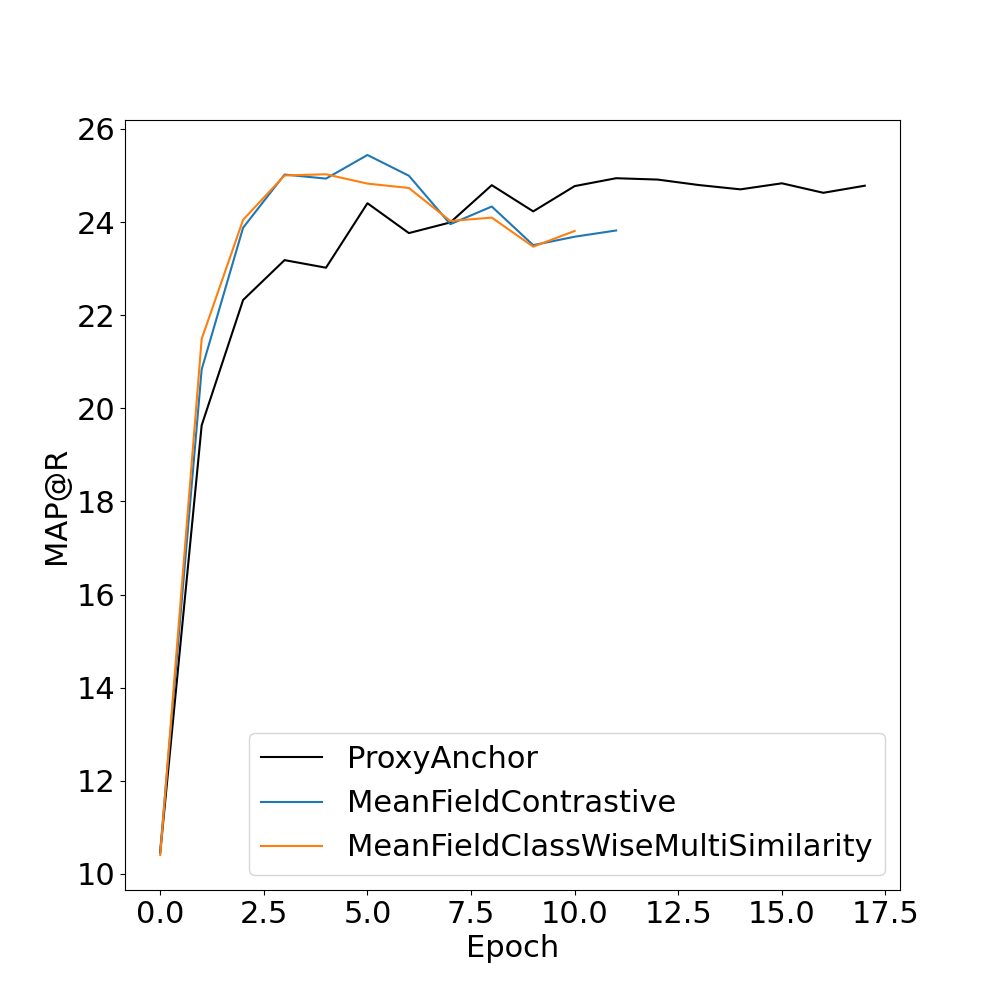
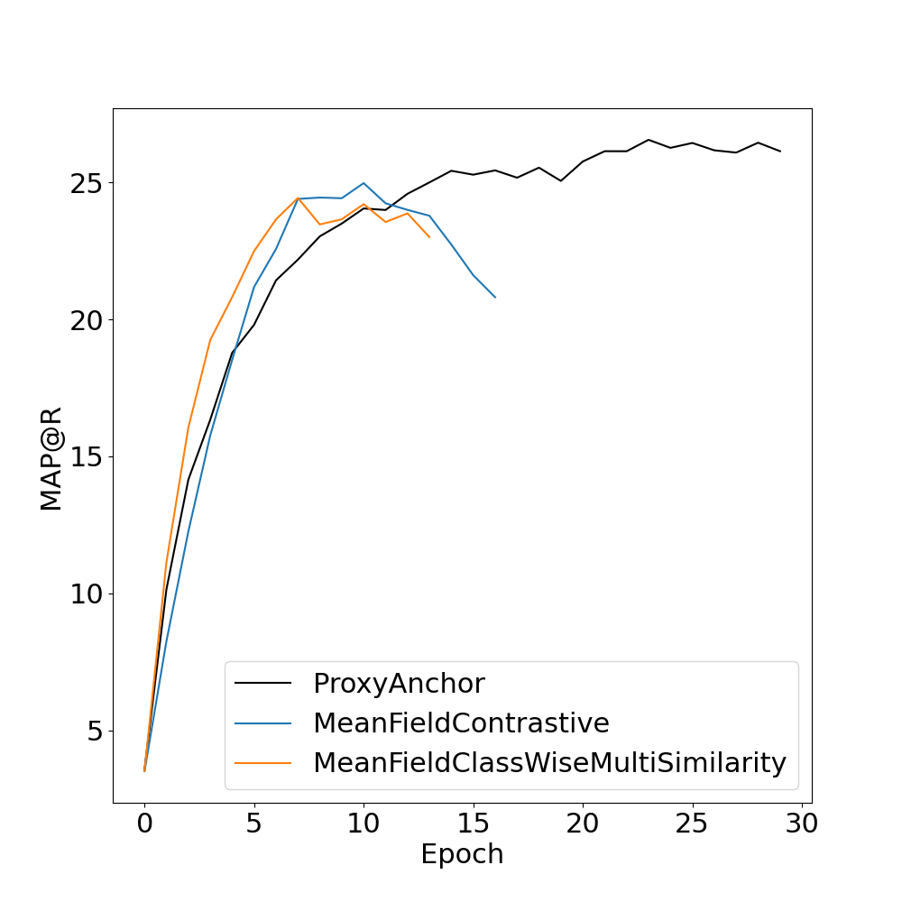
(a) CUB

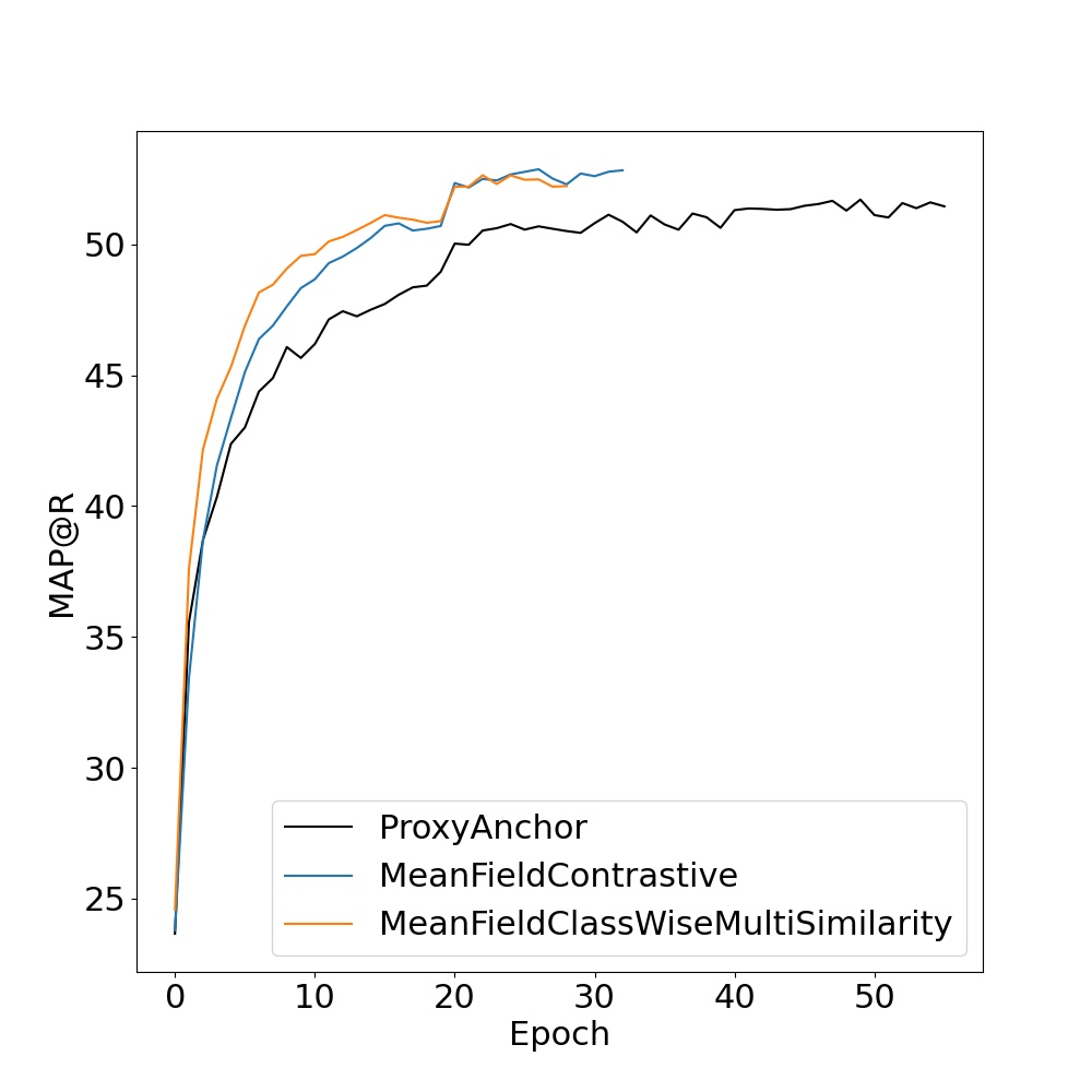
(b) Cars

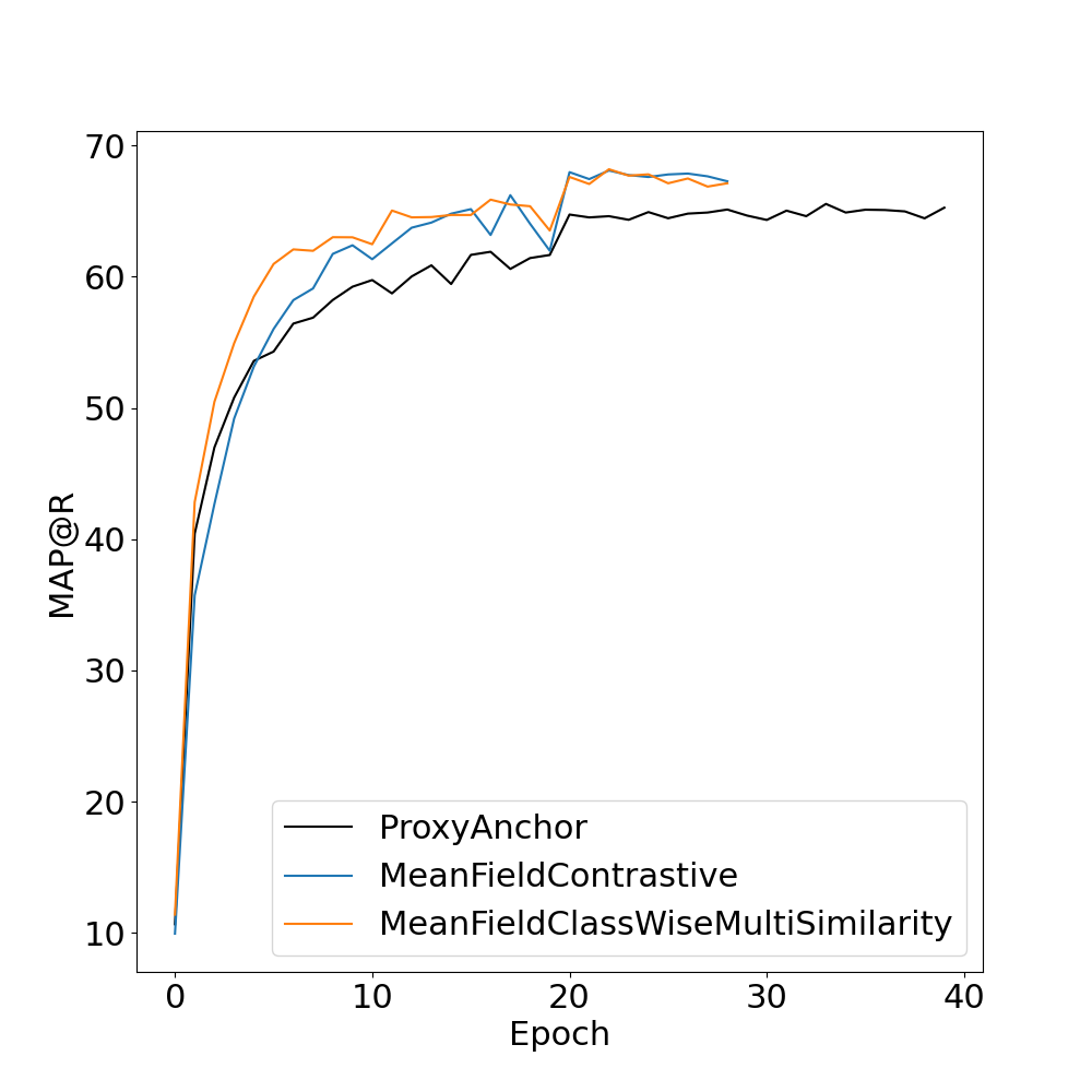
(c) SOP

(d) InShop

Figure 4: The test accuracy (MAP@R) plotted against the number of epochs for the (a) CUB, (b) Cars, (c) SOP, and (d) InShop datasets, comparing ProxyAnchor, MFCont., and MFCWMS.

Figure 4 shows learning curves obtained in the traditional evaluation protocol [6, 8] in fixed seeds, associated with Tables 2 and 3 in the main paper. Both MFCont. and MFCWMS losses show faster convergence than the ProxyAnchor loss. In the smaller datasets (CUB and Cars), accuracies of our mean field losses seem to decrease faster while we don’t see such behaviors in the larger datasets (SOP and InShop [35]). This phenomenon might be caused by strong repulsive interactions with negative mean fields. For larger datasets, the embedding spaces may be sufficiently populated to balance the repulsive force, while this may not be the case for smaller datasets. It might not occur for ProxyAnchor loss since repulsive forces for ProxyAnchor loss are weighted depending on distances between proxy and negative samples.

Impact of batch size in InShop.

Table 10 compares the MAP@R in ProxyAnchor and MFCWMS losses in the InShop dataset varying the batch size. As mentioned in the main paper, the accuracy of ProxyAnchor starts to decrease gradually for large batch sizes, while that of MFCWMS loss drops at batch size $150$. Moreover, Table 11 shows the MAP@R in ProxyAnchor and MFCWMS for the InShop dataset without the query–gallery split of test data. In this case, accuracies of both losses start to decrease gradually around batch size $150$. Thus, the accuracy drop for the MFCWMS loss in Table 10 probably comes from the specific query–gallery split.

Table 7: MLRC evaluation results in CUB-200-2011 [33]. We carry out $10$ test runs and show averaged metrics with their confidence intervals.

	Separated ($128$D)			Concatenated ($512$D)
Loss	MAP@R	P@1	RP	MAP@R	P@1	RP
ArcFace	${21.46\pm 0.13}$	${59.98\pm 0.22}$	${32.31\pm 0.14}$	${26.39\pm 0.16}$	${67.11\pm 0.23}$	${37.23\pm 0.17}$
CosFace	${21.19\pm 0.22}$	${59.74\pm 0.28}$	${32.00\pm 0.23}$	$\mathbf{26.54\pm 0.29}$	${67.14\pm 0.29}$	$\mathbf{37.38\pm 0.28}$
MS	${20.98\pm 0.16}$	${59.38\pm 0.27}$	${31.84\pm 0.15}$	${26.20\pm 0.16}$	${67.34\pm 0.35}$	${36.99\pm 0.16}$
MS+Miner	${20.78\pm 0.17}$	${59.02\pm 0.25}$	${31.67\pm 0.16}$	${25.94\pm 0.18}$	${67.08\pm 0.32}$	${36.77\pm 0.16}$
ProxyNCA	${18.75\pm 0.18}$	${57.06\pm 0.27}$	${29.64\pm 0.21}$	${23.84\pm 0.22}$	${65.60\pm 0.28}$	${34.82\pm 0.25}$
ProxyAnch.	$\mathbf{21.67\pm 0.22}$	$\underline{\mathbf{60.80\pm 0.33}}$	$\mathbf{32.53\pm 0.23}$	${26.48\pm 0.23}$	$\mathbf{67.72\pm 0.30}$	${37.30\pm 0.23}$
Cont.	${21.02\pm 0.14}$	${59.35\pm 0.33}$	${31.80\pm 0.15}$	${26.37\pm 0.18}$	$\mathbf{67.67\pm 0.25}$	${37.10\pm 0.19}$
MFCont.	$\mathbf{22.01\pm 0.10}$	$\mathbf{60.29\pm 0.23}$	$\mathbf{32.85\pm 0.10}$	$\underline{\mathbf{27.16\pm 0.07}}$	${67.64\pm 0.27}$	$\underline{\mathbf{37.95\pm 0.07}}$
CWMS	${21.48\pm 0.27}$	${60.09\pm 0.27}$	${32.32\pm 0.26}$	${26.94\pm 0.29}$	$\underline{\mathbf{68.24\pm 0.42}}$	${37.69\pm 0.27}$
MFCWMS	$\underline{\mathbf{22.11\pm 0.08}}$	$\mathbf{60.28\pm 0.10}$	$\underline{\mathbf{32.96\pm 0.08}}$	$\mathbf{27.03\pm 0.12}$	${67.63\pm 0.21}$	$\mathbf{37.83\pm 0.12}$

Table 8: MLRC evaluation results in Cars-196 [34]. We carry out $10$ test runs and show averaged metrics with their confidence intervals.

	Separated ($128$D)			Concatenated ($512$D)
Loss	MAP@R	P@1	RP	MAP@R	P@1	RP
ArcFace	${18.25\pm 0.12}$	${71.12\pm 0.36}$	${28.63\pm 0.13}$	$\mathbf{27.63\pm 0.15}$	${84.39\pm 0.15}$	$\mathbf{37.45\pm 0.15}$
CosFace	${18.49\pm 0.13}$	${74.66\pm 0.21}$	${28.75\pm 0.12}$	${26.96\pm 0.25}$	${85.29\pm 0.26}$	${36.80\pm 0.24}$
MS	${18.66\pm 0.30}$	${71.89\pm 0.33}$	${29.42\pm 0.29}$	${27.19\pm 0.41}$	${84.03\pm 0.30}$	${37.39\pm 0.36}$
MS+Miner	${18.49\pm 0.23}$	${71.99\pm 0.28}$	${29.20\pm 0.23}$	${26.89\pm 0.38}$	${83.89\pm 0.36}$	${37.09\pm 0.33}$
ProxyNCA	${17.43\pm 0.11}$	${70.96\pm 0.26}$	${27.85\pm 0.10}$	${26.78\pm 0.18}$	${84.31\pm 0.24}$	${36.83\pm 0.17}$
ProxyAnch.	$\underline{\mathbf{19.44\pm 0.17}}$	$\underline{\mathbf{76.15\pm 0.25}}$	$\mathbf{29.89\pm 0.18}$	${26.81\pm 0.27}$	$\underline{\mathbf{85.53\pm 0.30}}$	${36.76\pm 0.26}$
Cont.	${17.04\pm 0.26}$	${69.77\pm 0.40}$	${27.48\pm 0.26}$	${24.93\pm 0.46}$	${81.87\pm 0.35}$	${35.12\pm 0.42}$
MFCont.	$\mathbf{18.12\pm 0.13}$	$\mathbf{71.77\pm 0.28}$	$\mathbf{28.54\pm 0.14}$	$\mathbf{27.37\pm 0.18}$	$\mathbf{84.56\pm 0.21}$	$\mathbf{37.19\pm 0.18}$
CWMS	$\mathbf{19.27\pm 0.26}$	$\mathbf{74.19\pm 0.30}$	$\underline{\mathbf{29.95\pm 0.25}}$	$\underline{\mathbf{27.80\pm 0.33}}$	$\mathbf{85.18\pm 0.28}$	$\underline{\mathbf{37.89\pm 0.29}}$
MFCWMS	${18.85\pm 0.16}$	${73.02\pm 0.20}$	${29.55\pm 0.15}$	${26.98\pm 0.31}$	${84.00\pm 0.22}$	${37.11\pm 0.27}$

Table 9: MLRC evaluation results in Stanford Online Products [12]. We carry out $10$ test runs and show averaged metrics with their confidence intervals. We remove ProxyAnchor because it failed to converge in our settings.

	Separated ($128$D)			Concatenated ($512$D)
Loss	MAP@R	P@1	RP	MAP@R	P@1	RP
ArcFace	${41.47\pm 0.24}$	${71.39\pm 0.20}$	${44.35\pm 0.23}$	$\mathbf{47.37\pm 0.23}$	$\mathbf{76.13\pm 0.16}$	$\mathbf{50.22\pm 0.22}$
CosFace	${41.01\pm 0.24}$	${71.03\pm 0.22}$	${43.89\pm 0.24}$	${46.77\pm 0.20}$	${75.69\pm 0.13}$	${49.63\pm 0.20}$
MS	${41.87\pm 0.21}$	${71.10\pm 0.18}$	${45.00\pm 0.20}$	${46.70\pm 0.18}$	${75.21\pm 0.15}$	${49.70\pm 0.17}$
MS+Miner	${41.90\pm 0.30}$	${71.08\pm 0.25}$	${45.05\pm 0.30}$	${46.57\pm 0.28}$	${75.09\pm 0.19}$	${49.57\pm 0.28}$
ProxyNCA	$\mathbf{42.73\pm 0.11}$	$\mathbf{71.77\pm 0.08}$	$\mathbf{45.72\pm 0.11}$	${46.73\pm 0.13}$	${75.24\pm 0.10}$	${49.61\pm 0.13}$
Cont.	${41.09\pm 0.18}$	${70.04\pm 0.16}$	${44.18\pm 0.19}$	${45.35\pm 0.19}$	${73.88\pm 0.15}$	${48.28\pm 0.19}$
MFCont.	$\mathbf{43.62\pm 0.36}$	$\mathbf{72.74\pm 0.29}$	$\mathbf{46.55\pm 0.35}$	$\mathbf{47.01\pm 0.21}$	$\mathbf{75.57\pm 0.16}$	$\mathbf{49.85\pm 0.20}$
CWMS	${41.53\pm 0.20}$	${70.76\pm 0.16}$	${44.50\pm 0.21}$	${45.13\pm 0.16}$	${73.99\pm 0.11}$	${47.99\pm 0.16}$
MFCWMS	$\underline{\mathbf{44.57\pm 0.16}}$	$\underline{\mathbf{73.32\pm 0.11}}$	$\underline{\mathbf{47.53\pm 0.16}}$	$\underline{\mathbf{48.33\pm 0.18}}$	$\underline{\mathbf{76.38\pm 0.14}}$	$\underline{\mathbf{51.17\pm 0.18}}$

Table 10: Test accuracies on InShop with the test dataset split into queries and galleries.

Batch size	ProxyAnchor	MFCWMS
${30}$	${63.6\pm 1.4}$	${67.4\pm 0.2}$
${60}$	$\mathbf{65.7\pm 0.2}$	${67.6\pm 0.2}$
${90}$	${65.5\pm 0.3}$	${67.6\pm 0.2}$
${120}$	${65.6\pm 0.3}$	$\mathbf{67.8\pm 0.2}$
${150}$	${65.5\pm 0.2}$	${67.0\pm 0.6}$
${300}$	${64.5\pm 0.2}$	${67.0\pm 0.4}$
${500}$	${63.3\pm 0.2}$	${67.1\pm 0.1}$

Table 11: Test accuracies on InShop with the test dataset not split into queries and galleries.

Batch size	ProxyAnchor	MFCWMS
${30}$	${61.7\pm 0.6}$	${64.7\pm 0.1}$
${60}$	${62.8\pm 0.4}$	$\mathbf{65.1\pm 0.2}$
${90}$	$\mathbf{62.9\pm 0.3}$	${65.0\pm 0.5}$
${120}$	$\mathbf{62.9\pm 0.3}$	${64.9\pm 0.5}$
${150}$	${62.7\pm 0.1}$	${65.0\pm 0.4}$
${300}$	${61.9\pm 0.2}$	${64.7\pm 0.4}$
${500}$	${60.6\pm 0.2}$	${64.6\pm 0.1}$

References

- Wang et al. [2014] Jiang Wang, Yang Song, Thomas Leung, Chuck Rosenberg, Jingbin Wang, James Philbin, Bo Chen, and Ying Wu. Learning fine-grained image similarity with deep ranking. In Proceedings of the IEEE conference on computer vision and pattern recognition, pages 1386–1393, 2014.
- Schroff et al. [2015] Florian Schroff, Dmitry Kalenichenko, and James Philbin. Facenet: A unified embedding for face recognition and clustering. In Proceedings of the IEEE conference on computer vision and pattern recognition, pages 815–823, 2015.
- Hermans et al. [2017] Alexander Hermans, Lucas Beyer, and Bastian Leibe. In defense of the triplet loss for person re-identification. arXiv preprint arXiv:1703.07737, 2017.
- Anderson [1972] Philip W Anderson. More is different: broken symmetry and the nature of the hierarchical structure of science. Science, 177(4047):393–396, 1972.
- Weiss [1907] Pierre Weiss. L’hypothèse du champ moléculaire et la propriété ferromagnétique. J. Phys. Theor. Appl., 6(1):661–690, 1907.
- Movshovitz-Attias et al. [2017] Yair Movshovitz-Attias, Alexander Toshev, Thomas K Leung, Sergey Ioffe, and Saurabh Singh. No fuss distance metric learning using proxies. In Proceedings of the IEEE international conference on computer vision, pages 360–368, 2017.
- Musgrave et al. [2020a] Kevin Musgrave, Serge Belongie, and Ser-Nam Lim. A metric learning reality check. In Computer Vision–ECCV 2020: 16th European Conference, Glasgow, UK, August 23–28, 2020, Proceedings, Part XXV 16, pages 681–699. Springer, 2020a.
- Kim et al. [2020] Sungyeon Kim, Dongwon Kim, Minsu Cho, and Suha Kwak. Proxy anchor loss for deep metric learning. In Proceedings of the IEEE/CVF Conference on Computer Vision and Pattern Recognition, pages 3238–3247, 2020.
- Hadsell et al. [2006] Raia Hadsell, Sumit Chopra, and Yann LeCun. Dimensionality reduction by learning an invariant mapping. In 2006 IEEE Computer Society Conference on Computer Vision and Pattern Recognition (CVPR’06), volume 2, pages 1735–1742. IEEE, 2006.
- Weinberger and Saul [2009] Kilian Q Weinberger and Lawrence K Saul. Distance metric learning for large margin nearest neighbor classification. Journal of machine learning research, 10(2), 2009.
- Sohn [2016] Kihyuk Sohn. Improved deep metric learning with multi-class n-pair loss objective. Advances in neural information processing systems, 29, 2016.
- Oh Song et al. [2016] Hyun Oh Song, Yu Xiang, Stefanie Jegelka, and Silvio Savarese. Deep metric learning via lifted structured feature embedding. In Proceedings of the IEEE conference on computer vision and pattern recognition, pages 4004–4012, 2016.
- Wang et al. [2019a] Xinshao Wang, Yang Hua, Elyor Kodirov, Guosheng Hu, Romain Garnier, and Neil M Robertson. Ranked list loss for deep metric learning. In Proceedings of the IEEE/CVF conference on computer vision and pattern recognition, pages 5207–5216, 2019a.
- Wang et al. [2019b] Xun Wang, Xintong Han, Weilin Huang, Dengke Dong, and Matthew R Scott. Multi-similarity loss with general pair weighting for deep metric learning. In Proceedings of the IEEE/CVF conference on computer vision and pattern recognition, pages 5022–5030, 2019b.
- Shi et al. [2016] Hailin Shi, Yang Yang, Xiangyu Zhu, Shengcai Liao, Zhen Lei, Weishi Zheng, and Stan Z Li. Embedding deep metric for person re-identification: A study against large variations. In Computer Vision–ECCV 2016: 14th European Conference, Amsterdam, The Netherlands, October 11–14, 2016, Proceedings, Part I 14, pages 732–748. Springer, 2016.
- Wu et al. [2017] Chao-Yuan Wu, R Manmatha, Alexander J Smola, and Philipp Krahenbuhl. Sampling matters in deep embedding learning. In Proceedings of the IEEE international conference on computer vision, pages 2840–2848, 2017.
- Yuan et al. [2017] Yuhui Yuan, Kuiyuan Yang, and Chao Zhang. Hard-aware deeply cascaded embedding. In Proceedings of the IEEE international conference on computer vision, pages 814–823, 2017.
- Harwood et al. [2017] Ben Harwood, Vijay Kumar BG, Gustavo Carneiro, Ian Reid, and Tom Drummond. Smart mining for deep metric learning. In Proceedings of the IEEE International Conference on Computer Vision, pages 2821–2829, 2017.
- Wang et al. [2017] Feng Wang, Xiang Xiang, Jian Cheng, and Alan Loddon Yuille. Normface: L2 hypersphere embedding for face verification. In Proceedings of the 25th ACM international conference on Multimedia, pages 1041–1049, 2017.
- Zhai and Wu [2018] Andrew Zhai and Hao-Yu Wu. Classification is a strong baseline for deep metric learning. arXiv preprint arXiv:1811.12649, 2018.
- Liu et al. [2017] Weiyang Liu, Yandong Wen, Zhiding Yu, Ming Li, Bhiksha Raj, and Le Song. Sphereface: Deep hypersphere embedding for face recognition. In Proceedings of the IEEE conference on computer vision and pattern recognition, pages 212–220, 2017.
- Deng et al. [2019] Jiankang Deng, Jia Guo, Niannan Xue, and Stefanos Zafeiriou. Arcface: Additive angular margin loss for deep face recognition. In Proceedings of the IEEE/CVF conference on computer vision and pattern recognition, pages 4690–4699, 2019.
- Wang et al. [2018a] Feng Wang, Jian Cheng, Weiyang Liu, and Haijun Liu. Additive margin softmax for face verification. IEEE Signal Processing Letters, 25(7):926–930, 2018a.
- Wang et al. [2018b] Hao Wang, Yitong Wang, Zheng Zhou, Xing Ji, Dihong Gong, Jingchao Zhou, Zhifeng Li, and Wei Liu. Cosface: Large margin cosine loss for deep face recognition. In Proceedings of the IEEE conference on computer vision and pattern recognition, pages 5265–5274, 2018b.
- Zhu et al. [2020] Yuehua Zhu, Muli Yang, Cheng Deng, and Wei Liu. Fewer is more: A deep graph metric learning perspective using fewer proxies. In H. Larochelle, M. Ranzato, R. Hadsell, M.F. Balcan, and H. Lin, editors, Advances in Neural Information Processing Systems, volume 33, pages 17792–17803, 2020.
- Yang et al. [2022] Zhibo Yang, Muhammet Bastan, Xinliang Zhu, Douglas Gray, and Dimitris Samaras. Hierarchical proxy-based loss for deep metric learning. In Proceedings of the IEEE/CVF Winter Conference on Applications of Computer Vision, pages 1859–1868, 2022.
- Qian et al. [2019] Qi Qian, Lei Shang, Baigui Sun, Juhua Hu, Hao Li, and Rong Jin. Softtriple loss: Deep metric learning without triplet sampling. In Proceedings of the IEEE/CVF International Conference on Computer Vision, pages 6450–6458, 2019.
- Teh et al. [2020] Eu Wern Teh, Terrance DeVries, and Graham W Taylor. Proxynca++: Revisiting and revitalizing proxy neighborhood component analysis. In Computer Vision–ECCV 2020: 16th European Conference, Glasgow, UK, August 23–28, 2020, Proceedings, Part XXIV 16, pages 448–464. Springer, 2020.
- Li et al. [2022] Aoyu Li, Ikuro Sato, Kohta Ishikawa, Rei Kawakami, and Rio Yokota. Informative sample-aware proxy for deep metric learning. In Proceedings of the 4th ACM International Conference on Multimedia in Asia, pages 1–11, 2022.
- Nishimori and Ortiz [2010] Hidetoshi Nishimori and Gerardo Ortiz. Elements of phase transitions and critical phenomena. Oup Oxford, 2010.
- Paszke et al. [2019] Adam Paszke, Sam Gross, Francisco Massa, Adam Lerer, James Bradbury, Gregory Chanan, Trevor Killeen, Zeming Lin, Natalia Gimelshein, Luca Antiga, et al. Pytorch: An imperative style, high-performance deep learning library. Advances in neural information processing systems, 32, 2019.
- Musgrave et al. [2020b] Kevin Musgrave, Serge J. Belongie, and Ser-Nam Lim. Pytorch metric learning. ArXiv, abs/2008.09164, 2020b.
- Wah et al. [2011] Catherine Wah, Steve Branson, Peter Welinder, Pietro Perona, and Serge Belongie. The caltech-ucsd birds-200-2011 dataset. 2011.
- Krause et al. [2013] Jonathan Krause, Michael Stark, Jia Deng, and Li Fei-Fei. 3d object representations for fine-grained categorization. In Proceedings of the IEEE international conference on computer vision workshops, pages 554–561, 2013.
- Liu et al. [2016] Ziwei Liu, Ping Luo, Shi Qiu, Xiaogang Wang, and Xiaoou Tang. Deepfashion: Powering robust clothes recognition and retrieval with rich annotations. In Proceedings of the IEEE conference on computer vision and pattern recognition, pages 1096–1104, 2016.
- Ioffe and Szegedy [2015] Sergey Ioffe and Christian Szegedy. Batch normalization: Accelerating deep network training by reducing internal covariate shift. In International conference on machine learning, pages 448–456. pmlr, 2015.
- Russakovsky et al. [2015] Olga Russakovsky, Jia Deng, Hao Su, Jonathan Krause, Sanjeev Satheesh, Sean Ma, Zhiheng Huang, Andrej Karpathy, Aditya Khosla, Michael Bernstein, et al. Imagenet large scale visual recognition challenge. International journal of computer vision, 115:211–252, 2015.
- Loshchilov and Hutter [2017] Ilya Loshchilov and Frank Hutter. Decoupled weight decay regularization. arXiv preprint arXiv:1711.05101, 2017.