Heavy-tailed max-linear structural equation models in networks with hidden nodes

Abstract

Recursive max-linear vectors provide models for the causal dependence between large values of observed random variables as they are supported on directed acyclic graphs (DAGs). But the standard assumption that all nodes of such a DAG are observed is often unrealistic. We provide necessary and sufficient conditions that allow for a partially observed vector from a regularly varying model to be represented as a recursive max-linear (sub-)model. Our method relies on regular variation and the minimal representation of a recursive max-linear vector. Here the max-weighted paths of a DAG play an essential role. Results are based on a scaling technique and causal dependence relations between pairs of nodes. In certain cases our method can also detect the presence of hidden confounders. Under a two-step thresholding procedure, we show consistency and asymptotic normality of the estimators. Finally, we study our method by simulation, and apply it to nutrition intake data.

AMS 2020 Subject Classifications: primary:    60G70;    62D20;    62G32;    62H22

Keywords: Bayesian network, directed acyclic graph, extreme value theory, recursive max-linear model, regular variation, structure learning.

1 Introduction and motivation

Extreme value theory (EVT) has become indispensable for studying rare events, with particular applications to climate variables such as temperature, rainfall and flooding (Davison et al., 2019), storms and hurricanes (Davis et al., 2013; de Fondeville and Davison, 2022), and to financial disasters (Embrechts et al., 1997; Poon et al., 2004). Statistical modelling of such phenomena can improve our understanding of their underlying mechanisms and thus can suggest how to mitigate their effects. The modelling of multivariate extremes is a focus of active research, where the nonparametric character of joint distributions of extremes (Beirlant et al., 2004, Ch. 8, 9) has led to many directions of research, including spatial extremes (Davison et al., 2019), Bayesian modelling (e.g., Opitz et al., 2018) and graphical modelling (Engelke and Hitz, 2020; Gissibl and Klüppelberg, 2018).

High dimensionality and the limited number of rare events pose challenges for extreme dependence modelling, so most applications concern low-to-moderate dimensional settings (Engelke and Volgushev, 2023). Some exceptions are Chautru (2015) and Janßen and Wan (2020), who propose clustering approaches, Cooley and Thibaud (2019), who develop a decomposition method analogous to principal components analysis, Haug et al. (2015), whose approach is more akin to factor analysis, and Goix et al. (2016), who consider support detection for extremes. See Resnick (1987) and Resnick (2007) for an introduction and detailed treatment of multivariate EVT.

In this paper we discuss a class of graphical models for extremes using max-linear structural equation models in the sense of Pearl (2009) and introduced in Gissibl and Klüppelberg (2018). They are called recursive max-linear models (RMLMs) (Gissibl and Klüppelberg, 2018) or max-linear Bayesian networks (Amendola et al., 2022; Gissibl et al., 2021). A RMLM $\boldsymbol{X}$ supported on a directed acyclic graph (DAG) $\mathcal{D}=(V,E)$ with nodes $V=\{1,\dots,D\}$ and edges $E$ is defined as

$$X_{i}\coloneqq{\underset{k\in{\rm pa}(i)}{\bigvee}}c_{ik}X_{k}\vee c_{ii}Z_{i},\hskip 14.22636pt{i\in V},$$ (1.1)

for independent random variables $Z_{1},\dots,Z_{D}$ that have support $\mathbb{R}_{+}$ and are atomfree; the edge weights $c_{ik}$ are positive for all $i\in V$ and $k\in{\rm pa}(i)$, the parents of node $i$. These are arranged into the edge-weight matrix $C=(c_{ik})_{D\times D}$. We call such variables $Z_{1},\dots,Z_{D}$ innovations and call $\boldsymbol{Z}=(Z_{1},\dots,Z_{D})$ the innovations vector. Max-linearity offers an analogue to linear operations when analysing the influence of the largest shocks in a system.

Max-linear models have some appealing properties relative to other (linear) models. By construction, such models largely ignore the effect of weaker shocks, since it is mainly the extreme shocks that disseminate through the network. Hence, such models allow certain nodes to be identified as having primary influences on the other components. Moreover, max-linear models approximate any max-stable dependence structure between extremes arbitrarily well as the number of factors grows, making them an interesting and useful object of study in EVT; see, e.g., Fougerès et al. (2013) and Wang and Stoev (2011).

Identifiability and estimation for RMLMs are studied in Gissibl et al. (2021); Klüppelberg and Lauritzen (2020), and under the assumption of one-sided multiplicative noise in Buck and Klüppelberg (2021). Conditional independence under the RMLM is studied in Amendola et al. (2022), who introduce a new separation concept. Tran et al. (2022) propose a machine-learning algorithm for identifying the edges of a RMLM supported on a root-directed tree. Other work studying a max-linear model in the context of trees of transitive tournaments can be found in Asenova and Segers (2022).

Engelke and coauthors have followed a different approach towards graphical modelling for extremes. Engelke and Hitz (2020) use conditional independence relations in undirected graphical models for extremes when the exponent measure has a density. Engelke et al. (2022) build on this to propose a graph learning procedure for the Hüsler–Reiss model. Under the assumption of a graphical tree structure with undirected edges, Engelke and Volgushev (2023) develop a structure learning method for estimating the edges. Focusing on linear structural equation models with heavy tails, Gnecco et al. (2020) propose a structure learning method using conditional means of the integral transforms of pairs of node variables. Mhalla et al. (2020) propose a method for causal discovery by using Kolmogorov complexity and extreme conditional quantiles. Engelke and Ivanovs (2021) survey methods from some of the aforementioned references.

Analogous to the Gaussian setting, but focusing on extremes, Lee and Cooley (2022) and Gong et al. (2022) use partial tail correlations to infer undirected graphical structures.

1.1 Stating the problem

Structural equation models (SEMs) require assumptions about the observed variables. One particularly important assumption is that the errors or innovations are independent, which implies that the model is Markovian (Pearl, 2009, p.30). This ensures that the model satisfies the parental Markov condition, enabling one to read conditional independence relations from the graphical structure (Pearl, 2009, Theorem 1.4.1). However, this is also one of the most criticized assumptions, as one may not observe all relevant variables, resulting in unmeasured causes (Pearl, 2009, p. 252). Scenarios with hidden variables are common. In graphical terminology, these correspond to hidden confounders, i.e., variables which are unknown, undiscovered, or unmeasured. Ignoring their effects could lead to wrong conclusions.

Although structure learning procedures are concerned with inferring a causal order, i.e., a graph structure of the variables, few such procedures can handle situations with hidden nodes. To the best of our knowledge, there are just two publications in the literature on extremal graphical models dealing with similar problems. The approach in Gnecco et al. (2020, Section 4.1 below eq. (9)) may be used to identify a causal order even when there are hidden nodes. Similarly, but focusing on confounders only, Pasche et al. (2022) propose a way of testing whether there is a direct causal link between two variables. They model the scale parameter of the variables of interest by considering confounders in a regression setting.

Below we propose a different approach to detecting possible hidden nodes using specific properties of RMLMs. We focus on multivariate regularly varying RMLMs and find conditions under which one can ignore the effects of hidden nodes. In a RMLM there may be paths which are irrelevant, since, by max-linearity, extreme shocks will never pass through them. This property may even extend to certain nodes on irrelevant paths. Consequently, it is of no relevance whether such nodes are visible or hidden. We consider pairwise dependencies between any two observed node variables and provide necessary and sufficient conditions that allow us to check whether the observed variables can be modelled as a RMLM in the presence of hidden nodes.

Our work builds upon Klüppelberg and Krali (2021), who propose a scaling method to estimate the dependence structure of a RMLM, by first estimating a causal ordering of the nodes based on estimated scaling parameters, and then performing inference on the dependence parameters of the exponent measure of the regularly varying vector $\boldsymbol{X}$.

1.2 Terminology

We build on standard terminology for directed graphs (Lauritzen et al., 1990). Let $\mathcal{D}=(V,E)$ be a directed acyclic graph (DAG) with node set $V=\{1,\dots,{D}\}$ and edge set $E\subset V\times V$. For a node $i\in V$ the parents are ${\rm pa}(i)=\{j\in V:(j,i)\in E\}$ and ${\rm Pa}{(i)}={\rm pa}(i)\cup\{i\}$. Furthermore, let ${\rm an}(i)$ denote the ancestors of $i$ and let ${\rm An}(i)={\rm an}(i)\cup\{i\}$. Likewise, let ${\rm de}(i)$ be the descendants of $i$ and let ${\rm De}(i)={\rm de}(i)\cup\{i\}$. If $U\subseteq V$, then ${\rm an}(U)$ denotes the ancestral set of all nodes in $U$; ${\rm An}(U)={\rm an}(U)\cup U$, ${\rm de}(U)$ and ${\rm De}(U)$ are defined analogously. A node $i\in V$ is a source node if ${\rm pa}(i)=\emptyset$, and we denote the set of all source nodes by $V_{0}$. Let $j\to i$ denote an edge from node $j$ to node $i$. Then a path $p_{ji}\coloneqq[\ell_{0}=j\to\ell_{1}\to\cdots\to\ell_{m}=i]$ from $j$ to $i$ has length $|p_{ji}|=m$, and the set of all such paths is denoted by $P_{ji}$. Instead of $p_{ji}$ we also write simply $j\rightsquigarrow i$.

A graph $\mathcal{D}_{1}=(E_{1},V_{1})$ is called a subgraph of $\mathcal{D}$, if $V_{1}\subseteq V$ and $E_{1}\subseteq(V_{1}\times V_{1})\cap E$. If $\mathcal{D}$ is a DAG, then $\mathcal{D}_{1}$ is also a DAG.

A DAG $\mathcal{D}=(V,E)$ is well-ordered if for all $i\in V$ it is true that $i<j$ for all $j\in{\rm pa}(i)$. We refer to such an order as a causal order.

Recall that each node $j$ represents a random variable $X_{j}$ and we say $X_{j}$ causes $X_{i}$ (or $j$ causes $i$) whenever there is a path $j\rightsquigarrow i$.

Given nodes $i,j,k\in V$, we say that $X_{i}$ is a confounder of $X_{j}$ and $X_{k}$ (or $i$ is a confounder of $j$ and $k$) if there exist paths $i\rightsquigarrow j$ and $i\rightsquigarrow k$ which do not pass through $k,j$, respectively.

We close this subsection with the notions of endogenous and exogenous variables in structural equation models (Peters et al., 2014, p. 23–24). Endogenous variables are those that the modeler tries to understand (usually the $X_{i}$ in a RMLM) and exogeneous variables are independent and influence the endogenous variables, but are not influenced by them (the $Z_{i}$ in a RMLM).

1.3 A motivating example

Figure 1 shows three DAGs with node set $V=\{1,2,3\}$ and with node 3 hidden, i.e., we do not observe node 3, and may be unaware that it exists. The presence of a (dotted) edge between two nodes $j\to i$ ($j\in{\rm pa}(i)$) indicates that $c_{ij}>0$. Writing out eq. (1.1) for the three DAGs gives

$$X_{1}=c_{11}Z_{1}\vee c_{12}X_{2}\vee c_{13}X_{3},\quad X_{2}=c_{22}Z_{2}\vee c_{23}X_{3},\quad{X_{3}=c_{33}Z_{3}},$$ (1.2)

with $c_{13}=0$ for $\mathcal{D}_{1}$ and $c_{12}=0$ for $\mathcal{D}_{3}$. The problem we address in this paper is to find conditions that enable us to express $(X_{1},X_{2})$ as a RMLM of the form

$$X_{1}=c_{11}Z_{1}\vee c_{12}X_{2},\,\quad\quad X_{2}=\tilde{c}_{22}\tilde{Z}_{2},$$

for (independent) innovations $Z_{1},\tilde{Z}_{2}$. In Section 3 we prove that, under a regular variation condition on the innovations, the random variable $\tilde{Z}_{2}$ shares certain tail properties with $Z_{2}$.

Figure 1: Three-dimensional DAGs with hidden node 3, which is a confounder in $\mathcal{D}_{2}$ and $\mathcal{D}_{3}$.

To illustrate the notions of exogeneity and endogeneity, we reformulate (1.2) as

$$X_{1} =\left(c_{11}Z_{1}\vee c_{13}X_{3}\right)\vee c_{12}X_{2}\eqqcolon f_{13}(Z_{1},X_{3})\vee c_{12}X_{2},$$ (1.3)

$$X_{2} =c_{22}Z_{2}\vee c_{23}X_{3}\eqqcolon f_{23}(Z_{2},X_{3}),$$

and briefly discuss the three DAGs of Figure 1.

If, $c_{13}=0$, corresponding to $\mathcal{D}_{1}$, then $f_{13}=f_{13}(Z_{1})$ and $f_{23}=f_{23}(Z_{2},c_{33}Z_{3})$: both functions are exogenous, only depending on different innovations, which makes them independent. Extending the notion of innovations slightly, we call $f_{13}(Z_{1})$ and $f_{23}(Z_{2},c_{33}Z_{3})$ innovations of $(X_{1},X_{2})$. Indeed, $(X_{1},X_{2})$ is a RMLM on the smaller DAG $(\{1,2\},2\to 1)$.

If $c_{13}\neq 0$ and $c_{12}\neq 0$, corresponding to $\mathcal{D}_{2}$, then both $f_{13}$ and $f_{23}$ are functions of $X_{3}$ and thus not exogenous. Indeed, they can be written as functions of the innovations $f_{13}(Z_{1},c_{33}Z_{3})$ and $f_{23}(Z_{2},c_{33}Z_{3})$.

If $c_{12}=0$, corresponding to $\mathcal{D}_{3}$, then we have a situation similar to that for $\mathcal{D}_{2}$.

For $\mathcal{D}_{2}$ and $\mathcal{D}_{3}$ node 3 is a confounder of nodes 1 and 2 in the classical sense. For the DAG $\mathcal{D}_{2}$, under certain conditions on the path from 3 to 1 passing through 2, we are able to express $(X_{1},X_{2})$ as a RMLM (with independent innovations). It is the goal of this paper to investigate systematically when this is possible.

1.4 Recursive max-linear models

A RMLM $\boldsymbol{X}$ as defined in (1.1) has a unique solution, and the simplest way to derive it is via tropical algebra (see e.g. Butkovič, 2010), i.e., linear algebra with arithmetic in the max-times semiring $({\mathbb{R}}_{+},\vee,\times)$ defined by $a\vee b:=\max(a,b)$ and $a\times b:=ab$ for $a,b\in{\mathbb{R}}_{+}:=[0,\infty)$. The operations extend to ${\mathbb{R}}_{+}^{d}$ coordinatewise and to corresponding matrix multiplication $\times_{\max}$; see Amendola et al. (2022); Butkovič (2010) or Gissibl and Klüppelberg (2018) for more details. As usual in tropical or linear algebra, vectors are in general column vectors. For simplicity, we shall write $\boldsymbol{Z}=(Z_{1},\dots,Z_{D})$ for the innovations column vector. Tropical multiplication of the max-linear (ML) coefficient matrix $A$ with the innovations vector $\boldsymbol{Z}$ yields the unique solution (Gissibl and Klüppelberg, 2018, Theorem 2.2)

$$X_{i}=(A\times_{\max}\boldsymbol{Z})_{i}={{\underset{j\in{\rm An}(i)}{\bigvee}}}a_{ij}Z_{j},\hskip 14.22636pti\in\{1,\dots,D\}.$$ (1.4)

The matrix $A=(a_{ij})_{i,j\in\{1,\dots,D\}}$, called the ML coefficient matrix, is defined by the path weights, given for each path $p_{ji}=[j\to k_{1}\to\cdots\to k_{\ell}=i]$ as the product $d(p_{ji})=c_{jj}c_{k_{1}j}\cdots c_{ik_{\ell-1}}$. The entries of $A$ are defined for $i\in\{1,\dots,{D}\}$ by

$$a_{ij}=\underset{p_{ji}\in P_{ji}}{\bigvee}d(p_{ji})\mbox{ for }j\in{{\rm An}}(i),\quad a_{ij}=0\mbox{ for }j\in V\setminus{{\rm An}}(i),\quad a_{ii}=c_{ii}.$$

and a path $p_{ji}$ from $j$ to $i$ such that $a_{ij}={\bigvee}_{p_{ji}\in P_{ji}}d(p_{ji})$ is called max-weighted.

We use the following notion throughout the paper.

Definition 1.1.

For a pair of nodes $(i,m)$, we say that $(i,m)$ satisfies the max-weighted path property, if for all $u\in{\rm An}(i)\cap{\rm An}(m)$ there are max-weighted paths $u\rightsquigarrow m\rightsquigarrow i$. We summarize all such pairs in a set and write $(i,m)\in$ MWP. Note that $u=m$ is possible, so that this includes also max-weighted paths $m\rightsquigarrow i$.

Another important concept for RMLMs, derived from the matrix $A$ by restriction to a minimal number of edges, is that of the minimal max-linear DAG from Definition 5.1 of Gissibl and Klüppelberg (2018), which ignores all edges between any pairs of nodes that are not max-weighted paths.

Definition 1.2.

Let $\boldsymbol{X}$ be a recursive ML vector on a DAG $\mathcal{D}=(V,E)$ with ML coefficient matrix $A$. The DAG

$${\mathcal{D}_{A}=(V,E^{A})}\coloneqq\Big{(}V,\{(k,i)\in E:a_{ik}>\underset{\ell\in\rm{de}(k)\cap{\rm pa}(i)}{\bigvee}\frac{a_{i\ell}a_{\ell k}}{a_{\ell\ell}}\}\Big{)}$$

is called the minimum max-linear DAG of $\boldsymbol{X}$.

The DAG $\mathcal{D}_{A}$ defines the smallest subgraph of $\mathcal{D}$ such that $\boldsymbol{X}$ is a RMLM on this DAG.

1.5 Organisation

In Section 2 we provide conditions that ensure that a partially observed vector of node variables can be modelled as a RMLM. In Section 3, for a regular varying RMLM, we provide criteria based on max-weighted paths for the observed node variables to ensure the representation of such nodes as a RMLM, and derive conditions for the identification of max-weighted paths. In Section 4 we translate previous theoretical results into an estimation procedure, give an algorithm to detect max-weighted paths among the observed node variables, and apply our algorithm to interview data about food nutrition intake amounts.

The appendix has six sections. The main theorems of Sections 2 and 3 are proved in Appendix A. Appendix B summarizes standard definitions and results on regular variation, and specifies those relevant for RMLMs. Consistency and asymptotic normality of the estimated scalings and extreme dependence measures are proved in Appendix C, where we propose an intermediate thresholding procedure. This requires a functional central limit theorem for a random sample, which appears to be new. In Appendix D these results are used to estimate the inputs of our new algorithm. Appendix E investigates its performance in a simulation study based on true and false positive rates for the estimated max-weighted paths enriched by various categories of causal dependence. Appendix F gives details of our simulation results.

2 Constructing RMLMs from DAGs with hidden nodes

We now investigate the problem presented in Section 1.1 and motivated by the example of Section 1.3: given a RMLM $\boldsymbol{X}$ on a DAG $\mathcal{D}$ with $D$ nodes and certain nodes hidden, is it possible to construct a lower-dimensional RMLM on the observed $d<D$ nodes? We now show that under certain assumptions, concentrating on max-weighted paths, this may be possible.

2.1 Max-weighted paths and RMLMs on DAGs with hidden nodes

Suppose that the true DAG has $|V|={D}$ nodes, of which $d<D$ are observed. In this section we denote the set of observed nodes and its complement by $O\subset V$ and $O^{c}$, and write $\boldsymbol{X}_{O}$ for the vector of components with observed variables only.

A key tool is the minimal representation of the components of $\boldsymbol{X}$ (Gissibl and Klüppelberg, 2018, Theorem 6.7), where we replace the arbitrary subset of $V$ in that theorem by the subset $O\subset V$ of observed nodes. For $i\in V$ the sets can be reformulated as follows:

$${\rm An}^{O}(i) =\left\{j\in{\rm an}(i)\cap O:a_{ij}>\bigvee_{k\in O\cap\textrm{an}(i)\cap{\rm de}(j)}\frac{a_{ik}a_{kj}}{a_{kk}}\right\},$$

$${\rm An}^{O^{c}}(i) =\{i\}\cup\left\{j\in{\rm an}(i)\cap O^{c}:a_{ij}>\bigvee_{k\in O\cap{\rm an}(i)\cap{\rm de}(j)}\frac{a_{ik}a_{kj}}{a_{kk}}\right\}.$$ (2.1)

The set ${\rm An}^{O}(i)$, given in eq. (6.3) of Gissibl and Klüppelberg (2018), contains the lowest max-weighted ancestors of $i$ in $O$; i.e., those nodes $j$ such that no max-weighted path from $j$ to $i$ passes through any other node in $O$. Analogously, ${\rm An}^{O^{c}}(i)$ consists of the lowest max-weighted ancestors of $i$ in $O^{c}$ or $i$ itself. This allows us to express the ancestors of $i\in V$ in terms of the minimum numbers of observed nodes and of innovations. Hence, $X_{i}$ has minimal representation

$$X_{i} =\bigvee_{k\in{\rm An}^{O}(i)}\frac{a_{ik}}{a_{kk}}X_{k}\vee\bigvee_{k\in{\rm An}^{O^{c}}(i)}a_{ik}Z_{k},\quad{i\in V.}$$ (2.2)

As we are interested in this representation for $\boldsymbol{X}_{O}$ only, we use it for $i\in O$; then $\boldsymbol{X}_{O}$ is supported on the DAG $\mathcal{D}^{O}$ generated by representation (2.2).

Definition 2.1.

The DAG $\mathcal{D}^{O}$ induced by representation (2.2) with node set $O$ is called the observed DAG.

The following example illustrates the minimal representation (2.2).

Example 2.2.

Assume the situation as in $\mathcal{D}_{2}$ of Figure 1 with confounder 3 of nodes 1 and 2.

Then, if the path from $3\to 2\to 1$ is max-weighted, the path $3\to 1$ is irrelevant and equation (2.2) enables us to write $(X_{1},X_{2})$ as a RMLM with

$$X_{1}=a_{11}Z_{1}\vee\frac{a_{12}}{a_{22}}X_{2},\quad{X_{2}=a_{22}Z_{2}\vee a_{23}Z_{3}}=f_{23}(Z_{2},Z_{3}).$$

Extending the notion of innovations slightly, we call $Z_{1}$ and $f_{23}(Z_{2},Z_{3})$ innovations of $(X_{1},X_{2})$, since they can be written as functions of the original innovations only. They are both exogenous for $(X_{1},X_{2})$ as they involve independent innovations in both equations. Indeed, $(X_{1},X_{2})$ is a RMLM on the smaller DAG $(\{1,2\},2\to 1)$.

If the path $3\to 2\to 1$ is not max-weighted, then, as written in eq. (1.3), the new innovations $f_{13}(Z_{1},Z_{3})\coloneqq a_{11}Z_{1}\vee a_{13}Z_{3}$ and $f_{23}$ both depend on $Z_{3}$, which contradicts the independence of the innovations and hence $(X_{1},X_{2})$ can not be represented as a recursive ML vector.

The next theorem characterizes when a vector $\boldsymbol{X}_{O}$ of observed node variables can be represented as a RMLM. Part (i) characterizes the source nodes and part (ii) their descendants. The proof, which uses the representation (2.2), is deferred to Appendix A.

Theorem 2.3.

Let $\boldsymbol{X}\in{\mathbb{R}}_{+}^{D}$ be an arbitrarily ordered recursive ML vector with coefficient matrix $A\in\mathbb{R}_{+}^{D\times D}$. Let $O\subset V$ be the observed nodes. Then the vector $\boldsymbol{X}_{O}$ of observed variables can be represented as a recursive ML vector if and only if the following two conditions are satisfied:

1. For every $\ell\in O$ such that $O\cap{\rm an}(\ell)=\emptyset$ the following assertions hold:
   (a) ${\rm an}(\ell)\cap{\rm an}(j)=\emptyset$ for all $j\in O\cap{\rm de}(\ell)^{c}$;
   (b) there are max-weighted paths $u\rightsquigarrow\ell\rightsquigarrow i$ for all $i\in O\cap\emph{de}(\ell)$ and $u\in O^{c}\cap{\rm an}(\ell)\cap{\rm an}(i){=O^{c}\cap{\rm an}(\ell)}$.
   We denote the set of nodes $\ell$ satisfying these properties by $V_{0}^{O}$.

2. For every $u\in O^{c}\setminus\emph{an}(V_{0}^{O})$, and any pair $i,j\in O$ such that $u\in{\rm an}(i)\cap{\rm an}(j)$, either

   (a) if $j\in{\rm an}(i)$, there is a max-weighted path $u\rightsquigarrow j\rightsquigarrow i$, or there exists some $k\in{\rm an}(i)\cap{\rm an}(j)\cap O{={\rm an}(j)\cap O}$ such that there are max-weighted paths $u\rightsquigarrow k\rightsquigarrow i$ and $u\rightsquigarrow k\rightsquigarrow j$; or

   (b) if $j\notin{\rm an}(i)$, there exists some $k\in{\rm an}(i)\cap{\rm an}(j)\cap O$ such that there exist max-weighted paths $u\rightsquigarrow k\rightsquigarrow i$ and $u\rightsquigarrow k\rightsquigarrow j$.

Theorem 2.3 covers all three DAGs in Figure 1: For $\mathcal{D}_{1}$ there is a unique (hence max-weighted) path $1\rightsquigarrow 2\rightsquigarrow 3$ and Theorem 2.3(i, ii) is trivially satisfied. When node 3 is a confounder, then for $\mathcal{D}_{2}$ the vector $(X_{1},X_{2})$ can be represented as a RMLM provided $1\rightsquigarrow 2\rightsquigarrow 3$ is max-weighted. In contrast, this can never be done for $\mathcal{D}_{3}$.

The next example illustrates the conditions stated in Theorem 2.3 in a more complex setting.

Example 2.4.

Take a RMLM supported on the DAG in Figure 2 with $D=12$ nodes, of which $d=8$ nodes are observed and four are unobserved. Assume that $X_{12}=Z_{12}$ and $X_{11}=Z_{11}$.

Figure 2: Partially observed DAG with $12$ nodes, of which the four dotted nodes are hidden.

We wish to determine whether Theorem 2.3 can be used to write $X_{O}$ as a recursive ML vector. Note first from part (a) that $V_{0}^{O}\subseteq\{10,9,8\}$, as they have no ancestors in $O$. Moreover part (i)(a) holds for $\ell=10$. Hence, (i) holds if the paths $12\to 10\to 6$ and $12\to 10\rightsquigarrow 3$ are max-weighted. So assume that these hold such that part (i) of the theorem holds for $10\in V^{0}_{O}$.

We still need to check whether $9,8\in V^{O}_{0}$. However, as $8\notin{\rm de}(9)$ and $9\notin{\rm de}(8)$, the fact that ${\rm an}(9)\cap{\rm an}(8)\cap O^{c}=\{11\}$ contradicts Theorem 2.3 (i)(a). Hence, $X_{O}$ cannot be represented as a recursive ML vector, though it may nevertheless be possible to find a maximum subset of observed nodes that can be represented as a recursive ML vector. We present this below, after checking part (ii) of the theorem.

Candidates for $u$ are $\{5,7\}$ and $5\in{\rm an}(3)$ only, so 5 is not relevant for part (ii); however, $7\in{\rm an}(2)\cap{\rm an}(4)\cap{\rm an}(1)$ for observed nodes 2, 4 and 1. Hence, there are three pairs for $i,j$, namely $(4,2),(4,1)$, and $(2,1)$. As $4\in{\rm an}(2)$ we check part (ii)(a) and find the path $7\to 4\to 2$, the same applies to $4\in{\rm an}(1)$ with path $7\to 4\to 1$. As for the pair $(2,1)$, we check part (ii)(b) and find again the paths $7\to 4\to 2$ and $7\to 4\to 1$. Hence, part (ii) will be satisfied, provided both of these paths are max-weighted. If not, then Theorem 2.3 (ii) does not apply.

Suppose now that $11$ and none of the edges $11\to 9$ and $11\to 8$ exist, or equivalently that $c_{9,11}=c_{8,11}=0$. Define $D_{-11}=D\setminus\{11\}$ and the corresponding sub-DAG in Figure 2 without the edges $11\to 9$ and $11\to 8$. This decouples nodes 8 and 9, because ${\rm an}(8)={\rm an}(9)=\emptyset$, so (i)(a) holds trivially, and no $u$ exists in (i)(b). For part (ii) node 11 was irrelevant anyway.

We summarize all max-weighted path conditions needed to obtain a RMLM for $\boldsymbol{X}_{O}$ from this DAG:

1. $12\to 10\to 6$ and $12\to 10\rightsquigarrow 3$ are max-weighted, and

2. $7\to 4\to 1$, $7\to 4\to 2$ are max-weighted.

If the aforementioned conditions are satisfied and we also assume that the edge $10\to 3$ is max-weighted, then $\boldsymbol{X}_{O}$ is a RMLM supported on the observed DAG shown in Figure 3.

Figure 3: DAG $\mathcal{D}^{O}$ with the observed $8$ nodes, if node $11$ is absent and (a) and (b) hold.

The following remark may help to develop some intuition on the relation between Theorem 2.3 and representation (2.2).

Remark 2.5.

This remark connects Theorem 2.3 and representation (2.2). Assume the situation in Example 2.4 with the DAG in Figure 2. For each of the conditions of Theorem 2.3 we select a pair of nodes, and show how the exogeneity property of the innovations fails to hold when the max-weighted paths conditions (a) and (b) from the end of Example 2.4 are not satisfied.
$\bullet$   Condition $(i)(a)$ and candidates $\{8,9\}$ for source nodes: while $8\notin{\rm de}(9)$ , $9\notin{\rm de}(8)$, we have that ${\rm an}(9)\cap{\rm an}(8)\cap O^{c}=\{11\}$, and since $11\in O^{c}$, representation (2.2) yields

$$X_{9}=a_{99}Z_{9}\vee a_{9,11}Z_{11},\quad X_{8}=a_{88}Z_{8}\vee a_{8,11}Z_{11}.$$

As the innovations of $X_{9}$ and $X_{8}$ both depend on $Z_{11}$, they cannot be represented in a RMLM.

Suppose now that $11$ and none of the edges $11\to 9$ and $11\to 8$ exist, equivalently, that $c_{9,11}=c_{8,11}=0$. Then

$$X_{9}=a_{99}Z_{9},\quad X_{8}=a_{88}Z_{8},$$

such that the innovations are exogenous. In this case, also (i)(b) holds trivially since $({\rm an}(9)\cup{\rm an}(8))\cap O^{c}=\emptyset$, and thus $\{8,9\}\in V_{0}^{O}$.
$\bullet$   Condition $(i)(b)$ and candidate 10 for a source node. Consider the nodes $\{6,10\}$. Suppose that the edge $12\to 6$ is the only max-weighted path, then representation (2.2) yields

$$X_{10}=a_{10,10}Z_{10}\vee a_{10,12}Z_{12},\quad X_{6}=\frac{a_{6,10}}{a_{10,10}}X_{10}\vee a_{66}Z_{6}\vee a_{6,12}Z_{12}.$$

As the innovations of $X_{10}$ and $X_{6}$ both depend on $Z_{12}$, they cannot be represented in a RMLM.

If, instead, the path $12\to 10\to 6$ is the only max-weighted path, then representation (2.2) yields

$$X_{10}=a_{10,10}Z_{10}\vee a_{10,12}Z_{12},\quad X_{6}=\frac{a_{6,10}}{a_{10,10}}X_{10}\vee a_{66}Z_{6},$$

such that the innovations are exogenous. In this case, also (i)(b) holds trivially since ${\rm an}(10)\cap O^{c}=\emptyset$, and thus $10\in V_{0}^{O}$.
$\bullet$  Conditions (ii)(a), (ii)(b), with $u=7$ and node pairs $(4,2),(4,1)$, and $(2,1)$. Assume that the edge $7\to 2$ is the only max-weighted path, so by representation (2.2),

$$X_{4}=\frac{a_{48}}{a_{88}}X_{8}\vee\frac{a_{49}}{a_{99}}X_{9}\vee a_{44}Z_{4}\vee a_{47}Z_{7},\quad X_{2}=\frac{a_{24}}{a_{44}}X_{4}\vee\frac{a_{28}}{a_{88}}X_{8}\vee\frac{a_{29}}{a_{99}}X_{9}\vee a_{22}Z_{2}\vee a_{27}Z_{7}.$$

As the innovations of $X_{4}$ and $X_{2}$ both depend on $Z_{7}$, they cannot be represented as a RMLM. This also contradicts (ii)(a) with $u=7$ and $4\in{\rm an}(2)$.

A similar result holds if the edge $7\to 1$ is the only max-weighted path, since in this case $X_{4}$ is as above and

$$X_{1}=\frac{a_{19}}{a_{99}}X_{9}\vee\frac{a_{18}}{a_{88}}X_{8}\vee\frac{a_{14}}{a_{44}}X_{4}\vee a_{11}Z_{1}\vee a_{17}Z_{7}.$$

Then the innovations of $X_{4}$ and $X_{1}$ again both depend on $Z_{7}$, and they cannot be represented as a RMLM. This also contradicts (ii)(a) with $u=7$ and $4\in{\rm an}(1)$.

As for the pair $(1,2)$, which have no ancestral relation, we check (ii)(b) and find that $k=4$ is a candidate. However, if either $7\to 1$, or $7\to 2$, or both, are max-weighted, $(ii)(b)$ and the exogeneity of the innovations fail to hold for the pairs $(4,1)$, or $(4,2)$, respectively.

Suppose now that both paths $7\to 4\to 2$ and $7\to 4\to 1$ are max-weighted. This reduces the representation (2.2) to

$$X_{4}=\frac{a_{48}}{a_{88}}X_{8}\vee\frac{a_{49}}{a_{99}}X_{9}\vee a_{44}Z_{4}\vee a_{47}Z_{7},\quad X_{2}=\frac{a_{24}}{a_{44}}X_{4}\vee a_{22}Z_{2},\quad X_{1}=\frac{a_{14}}{a_{44}}X_{4}\vee a_{11}Z_{1},$$

and thus all innovations of the components of $(X_{1},X_{2},X_{4})$ are exogenous.

The following is a simple consequence of Theorem 2.3 for a root-directed tree, i.e., a tree with all edges directed to a single (root) node.

Corollary 2.6.

If the recursive ML vector $\boldsymbol{X}=(X_{1},\dots,X_{D})\in{\mathbb{R}}_{+}^{D}$ is supported on a root-directed tree and we observe $(X_{o_{1}},\ldots,X_{o_{d}})$ for $d<D$, where $o_{i}<o_{j}$ for $i<j$, then $(X_{o_{1}},\ldots,X_{o_{d}})$ is also a RMLM.

Proof.

Every node of such a tree has a single child, so a hidden node is never a confounder, and therefore (i) and (ii) in Theorem 2.3 are both satisfied. If the root node is also observed, then the observed RMLM is also supported on a root-directed tree. ∎

3 Regular variation of a recursive max-linear vector

3.1 Extremal dependence

In the rest of the paper we suppose that the innovations vector $\boldsymbol{Z}\in{\mathbb{R}}_{+}^{D}$ is regularly varying with index $\alpha>0$, written $\boldsymbol{Z}\in{\rm RV}_{+}^{D}(\alpha)$, and that it has independent and standardized components, with $n\mathds{P}(n^{-1/\alpha}Z_{i}>x)\to x^{-\alpha}$, $x>0$, as $n\to\infty$ for all $i\in\{1,\dots,{D}\}$. Then RMLMs as in (1.4) belong to the more general class of max-linear models with independent regularly varying innovations, which have a long history; see, for example, Wang and Stoev (2011), de Haan and Ferreira (2006, Chapter 6), or Resnick (1987, Chapter 5). They are multivariate regularly varying and have a discrete spectral measure $H_{\boldsymbol{X}}$ with normalized version $\tilde{H}_{\boldsymbol{X}}$. We define multivariate regular variation, its angular representation and its spectral measure in Appendix B, referring the reader to Resnick (1987, 2007) for more insight.

Our results depend on the following extreme dependence measure, introduced in Propositions 3 and 4 of Larsson and Resnick (2012); see also Cooley and Thibaud (2019, §4) and Klüppelberg and Krali (2021, §2.2) for more details.

Definition 3.1.

Let $\boldsymbol{X}\in{\rm RV}^{D}_{+}(2)$ and consider its angular representation $(R,\boldsymbol{\omega})$ as in Definition B.1(b), under which $\omega_{i}={X_{i}}/{R}$ for $i\in\{1,\dots,D\}$. For all $i,j\in\{1,\ldots,{D}\}$ define a measure of extreme dependence between $\omega_{i}$ and $\omega_{j}$ to be

$$\sigma_{ij}^{2}=\sigma_{X_{ij}}^{2} \coloneqq\int_{\Theta_{+}^{{{D}}-1}}\omega_{i}\omega_{j}{\rm d}H_{\boldsymbol{X}}(\boldsymbol{\omega}),\quad\boldsymbol{\omega}=(\omega_{1},\dots,\omega_{{D}})\in\Theta_{+}^{{{D}}-1}.$$

We write $\sigma_{i}=\sigma_{{X}_{i}}=\sigma_{{X}_{ii}}$ and call it the scaling parameter of $X_{i}$ or just the scaling.   $\Box$

The matrix $\Sigma\coloneqq(\sigma_{ij})_{D\times D}$ summarizes the structure of $\boldsymbol{X}$ in terms of second-order properties of its angular measure.

If we now focus on a RMLM (1.4), regular variation with ${\alpha}=2$ and the Euclidean norm $\|\cdot\|$, the matrix $\Sigma=AA^{\top}$ for $A\in{\mathbb{R}}^{D\times D}$ has row vectors $A_{i}$ and column vectors $a_{k}$ for $i,k\in\{1,\dots,D\}$. Proposition 3.2 establishes that the $a_{k}$ are the non-normalized atoms of the spectral measure $H_{\boldsymbol{X}}$.

Proposition 3.2.

Let ${\boldsymbol{X}}=A\times_{\max}\boldsymbol{Z}$, where $\boldsymbol{Z}\in{\rm RV}^{D}_{+}(2)$ is an innovations vector with standardized components, and $A\in\mathbb{R}^{{D}\times{D}}_{+}$. Then

1. the atoms of the spectral measure $H_{\boldsymbol{X}}$ of $\boldsymbol{X}$ are $(a_{k}/\lVert a_{k}\rVert){=(a_{k}/{(\sum_{i=1}^{D}a_{ik}^{2})^{1/2}})}$ for $k\in\{1,\dots,D\}$,

2. $\sigma_{ij}^{2}=(AA^{\top})_{ij}=\sum_{k=1}^{D}a_{ik}a_{jk}$ for $i,j\in\{1,\dots,D\}$, and

3. every component $X_{i}$ of $\boldsymbol{X}$ has squared scaling $\sigma^{2}_{i}=\sum_{k=1}^{D}a_{ik}^{2}$ for $i\in\{1,\dots,D\}$.

Finally, we consider the standardized recursive ML random vector $\boldsymbol{X}$ obtained from (1.4) by standardizing the ML coefficient matrix.

Definition 3.3.

The standardized ML coefficient matrix $\bar{A}$ is defined as

$$\bar{A}=(\bar{a}_{ij})_{{D}\times{D}}{=\bigg{(}\frac{a_{ij}}{\|A_{i}\|}\bigg{)}_{{D}\times{D}}}\coloneqq\bigg{(}\frac{a_{ij}^{2}}{\sum_{k\in\textrm{An(i)}}a_{ik}^{2}}\bigg{)}_{{D}\times{D}}^{1/2}=\bigg{(}\frac{a_{ij}^{2}}{\sum_{k=1}^{D}a_{ik}^{2}}\bigg{)}_{{D}\times{D}}^{1/2}.$$ (3.1)

Proposition 3.2 entails the following corollary for every standardized ML vector $\boldsymbol{X}$.

Corollary 3.4.

Let $\boldsymbol{X}=\bar{A}\times_{\max}\boldsymbol{Z}$. Then

1. the columns $(\bar{a}_{k})$ of $\bar{A}$ for $k\in\{1,\dots,D\}$ are the non-normalized atoms of the spectral measure $H_{\boldsymbol{X}}$ of the standardized vector $\boldsymbol{X}$,

2. $\sigma^{2}_{i}=(\bar{A}\bar{A}^{\top})_{ii}=1$, and

3. for $i\neq j$, $\sigma_{ij}^{2}=1\,\iff\,{\bar{a}_{ik}=\bar{a}_{jk}}$ for all $k\in\{1,\dots,D\}\,\iff\,X_{i},X_{j}$ are asymptotically fully dependent.

See Appendix B.1 for a precise definition and proof of the last equivalence of part (c).

Standardization also allows us to use Lemma 2.1 of Gissibl et al. (2018), re-stated below.

Lemma 3.5.

If the RMLM $\boldsymbol{X}$ is supported on a well-ordered DAG, then $\bar{a}_{jj}>\bar{a}_{ij}$ for $i\in V$ and $j\in{\rm an}(i)$.

We now summarize all model assumptions used throughout the rest of the paper.

Assumptions A:

1. The innovations vector $\boldsymbol{Z}\in{\rm RV}^{D}_{+}(2)$ has independent and standardized components.

2. The norm $\|\cdot\|$ denotes the Euclidean norm.

3. The ML coefficient matrix $A$ is standardized as in (3.1), so that the components of $\boldsymbol{X}$ are standardized.

In this paper we use the maximum over tuples of components of the vector $\boldsymbol{X}$ when Assumptions (A1)–(A3) are satisfied. Lemma 6 in Klüppelberg and Krali (2021), which we re-state below, characterizes the scalings of such objects in terms of the ML coefficient matrix.

Lemma 3.6.

Let $\boldsymbol{X}$ be a recursive ML vector satisfying assumptions (A1)–(A3). Then the random variable $M_{\boldsymbol{h}}\coloneqq\max(X_{i}:i\in\boldsymbol{h})$ is again max-linear. In particular $M_{\boldsymbol{h}}\in{\rm RV}_{+}(2)$ with squared scalings defined as follows:
(a) if $\boldsymbol{h}\subseteq\{1,\dots,{D}\}$, then $\sigma_{M_{\boldsymbol{h}}}^{2}=\sum_{k=1}^{D}\bigvee_{i\in\boldsymbol{h}}a_{ik}^{2}$; and
(b) if $\boldsymbol{h}=\{1,\dots,{D}\}$, then $\sigma_{M_{\boldsymbol{h}}}^{2}=\sum_{k=1}^{D}a_{kk}^{2}.$

3.2 The ML matrix of a RMLM with hidden nodes

Our previous setting assumes that $\boldsymbol{X}\in{\rm RV}_{+}^{D}$ is a RMLM with ML coefficient matrix $A\in{\mathbb{R}}_{+}^{D\times D}$, each row of which satisfies (1.4). However, only $d<D$ of the nodes of the DAG supporting $\boldsymbol{X}$ are observed, corresponding to a max-linear vector $\boldsymbol{X}_{O}=A_{O}\times_{\max}\boldsymbol{Z}\in{\mathbb{R}}_{+}^{d}$ with ML coefficient matrix $A_{O}\in{\mathbb{R}}^{d\times D}$, where the rows of $A_{O}$ correspond to the observed node variables in $O$. Regular variation results are unaffected by the dimension of $A_{O}$, and so remain valid for $\boldsymbol{X}_{O}$.

A natural question is whether it is possible to reduce the matrix $A_{O}$ to a square $d\times d$ matrix and the innovations vector to a vector of exogenous random variables in ${\mathbb{R}}_{+}^{d}$ with independent components in ${\rm RV}_{+}(2)$. To address this we start with a useful lemma.

Lemma 3.7.

If the innovations $Z_{1},\ldots,Z_{p}$ for $p\leq D$ satisfy Assumption (A1) and $(a_{1},\ldots,a_{p})$ $\in\mathbb{R}_{+}^{p}$, then the maximum $M\coloneqq\vee_{i\in\{1,\ldots,p\}}a_{i}Z_{i}$ belongs to ${\rm RV}_{+}(2)$ with squared scaling $\sigma^{2}=\sum_{i=1}^{p}a_{i}^{2}$. In particular, $M=\sigma Z$ where $Z\in{\rm RV}_{+}(2)$ and has unit scaling.

Proof.

Recall that ${\rm RV}_{+}(2)$ is closed with respect to max-linear combination. The scaling follows as in Lemma 3.6 (a), and defining $Z:=M/\sigma$ implies that $Z\in{\rm RV}_{+}(2)$ with unit scaling. ∎

We now illustrate via an example how closure under max-linear combinations becomes useful in reducing the dimension of the matrix $A_{O}$.

Example 3.8.

Consider a RMLM supported on the DAG $\mathcal{D}_{2}$ in Figure 1 and satisfying Assumptions (A1)–(A3). Furthermore, suppose that the path $3\to 2\to 1$ is max-weighted. We have $O=\{1,2\}$, $D=3$ and $d=2$ and hidden node 3, and the following reduced ML representation:

$$\begin{bmatrix}X_{1}\\ X_{2}\end{bmatrix} {=}\begin{bmatrix}a_{11}Z_{1}\vee a_{12}Z_{2}\vee a_{13}Z_{3}\\ a_{22}Z_{2}\vee a_{23}Z_{3}\end{bmatrix}\overset{}{=}\begin{bmatrix}a_{11}Z_{1}\vee(a_{12}/a_{22})X_{2}\\ a_{22}^{*}Z^{*}_{2}\end{bmatrix}\overset{}{=}\begin{bmatrix}a_{11}Z_{1}\vee(a_{12}a_{22}^{*}/a_{22})Z^{*}_{2}\\ a_{22}^{*}Z^{*}_{2}\end{bmatrix},$$ (3.2)

where $a_{22}^{*2}=a_{22}^{2}+a_{23}^{2}$, and $Z_{2}^{*}=(a_{22}Z_{2}\vee a_{23}Z_{3})/a_{22}^{*}$ is a standardized innovation following Lemma 3.7. Therefore, the new innovation vector is given by $(Z_{1},Z_{2}^{*})$ and the reduced ML coefficient matrix lies in $\mathbb{R}^{2\times 2}$.

The following result shows how to represent the max-linear vector $\boldsymbol{X}_{O}=A_{O}\times_{\max}\boldsymbol{Z}$ with $|O|=d$, ML coefficient matrix $A_{O}\in{\mathbb{R}}^{d\times D}$ and $\boldsymbol{Z}\in{\mathbb{R}}_{+}^{D}$ as a RMLM with reduced and upper-triangular ML coefficient matrix, provided the conditions of Theorem 2.3 are satisfied.

Proposition 3.9.

Suppose that $\boldsymbol{X}\in{\rm RV}_{+}^{D}(2)$ is a RMLM with ML coefficient matrix $A\in\mathbb{R}^{D\times D}$ satisfying Assumptions (A1)–(A3) and with $D\geq 2$. Assume that the observed nodes $\boldsymbol{X}_{O}$ have $|O|=d<D$ and satisfy conditions (i) and (ii) of Theorem 2.3. Then

$$\boldsymbol{X}_{O}=A_{O}^{*}\times_{\max}\boldsymbol{Z^{*}}$$ (3.3)

with innovations vector $\boldsymbol{Z}^{*}=(Z_{1}^{*},\dots,Z_{d}^{*})$ and reduced ML coefficient matrix

$$A_{O}^{*}=\begin{bmatrix}a^{*}_{11}&a^{*}_{12}&\ldots&a^{*}_{1d}\\ 0&a^{*}_{22}&\ldots&a^{*}_{2d}\\ \vdots&\vdots&\ddots&\vdots\\ 0&0&\ldots&a^{*}_{dd}\end{bmatrix},$$ (3.4)

where

$$a_{ii}^{*}=\Big{(}\sum_{k\in{\rm An}^{O^{c}}(i)}a_{ik}^{2}\Big{)}^{1/2},\qquad a_{ij}^{*}=\bigvee_{k\in{{\rm De}(j)}\cap{\rm An}^{O}(i)}\frac{a_{ik}}{a_{kk}}a_{kj}^{*},\quad{j>i},$$

and ${\rm An}^{O}(i)$ and ${\rm An}^{O^{c}}(i)$ are defined in (2.1).

Proof.

We consider only the observed nodes $O$ and proceed via induction over the generations of the DAG of the observed part $\boldsymbol{X}_{O}$ of the RMLM. The definition of these generations is quite intuitive; see Definition 1 of Klüppelberg and Krali (2021).

We start with the source nodes $V_{0}^{O}$. Now ${\rm An}(i)={\rm An}^{O^{c}}(i)$ for $i\in V^{O}_{0}$, and we find from (2.2) that

$$X_{i}=\bigvee_{k\in{\rm An}^{O^{c}}(i)}a_{ik}Z_{k}\,=\,a^{*}_{ii}Z^{*}_{i},$$ (3.5)

where $a_{ii}^{*2}=\sum_{j\in{\rm An}(i)}a_{ij}^{2}$, and $Z^{*}_{i}=\vee_{j\in{\rm An}{(i)}}(a_{ij}/a_{ii}^{*})Z_{j}$ by Lemma 3.7. Moreover $a_{ij}^{*2}=0$ for $j\neq i$ by Theorem 2.3 (i)(a), because the summation covers all ancestors of $X_{i}$. Furthermore the source nodes and hence $Z^{*}_{i}$ are independent by Theorem 2.3(i)(a). As $\boldsymbol{X}_{O}$ lives on a well-ordered DAG, the source nodes correspond to the last components of $\boldsymbol{X}_{O}$ and the corresponding rows in $A^{*}_{O}$ have non-zero entries only on the diagonal.

Now consider a node $i_{1}$ in generation $G_{1}^{O}$, which consists of the children of nodes in $V_{0}^{O}$ in $O$. By (2.2), we find

$$X_{i_{1}}{=}\bigvee_{k\in{\rm An}^{O}(i_{1})}\frac{a_{i_{1},k}}{a_{kk}}X_{k}\vee a_{i_{1},i_{1}}^{*}Z_{i_{1}}^{*},$$ (3.6)

where $a_{i_{1},i_{1}}^{*2}=\sum_{k\in{\rm An}^{O^{c}}(i_{1})}a_{i_{1},k}^{2}$ and, by Lemma 3.7, $Z^{*}_{i_{1}}=\vee_{j\in{\rm An}^{O^{c}}(i_{1})}Z_{j}/a_{i_{1},i_{1}}^{*}$.

We now show that $Z^{*}_{i_{1}}$ is independent, first, of $X_{k}\in V_{0}^{O}$ and, second, of $Z^{*}_{j_{1}}$, with $i_{1},j_{1}\in G_{1}^{O}$.

To prove the first, note that if $i_{1}\in G_{1}^{O}$ and $i\in V_{0}^{O}$ have a common hidden ancestor $u$, then by Theorem 2.3(i)(b) there must be a max-weighted path $u\rightsquigarrow i\rightsquigarrow i_{1}$. Therefore, representation (3.6) for $X_{i_{1}}$ contains $X_{i}$ in the first maximum, such that the innovations indexed in ${\rm An}^{O^{c}}(i)$ and ${\rm An}^{O^{c}}(i_{1})$ must have different indices, and therefore be independent.

To prove the second, we take two different nodes $i_{1},j_{1}\in G_{1}^{O}$. Then by Theorem 2.3 (ii)(b), any max-weighted path to $i_{1}$ and $j_{1}$ from a common hidden ancestor would have to pass through a common source node variable $X_{k}$ for $k\in V_{0}^{O}\cap{\rm pa}^{O}(i_{1})\cap{\rm pa}^{O}(j_{1})$. Hence, in representations (3.6) for $X_{i_{1}}$ and $X_{j_{1}}$, the innovations would be the scaled innovations with different indices in ${\rm An}^{O^{c}}(i_{1})$ and ${\rm An}^{O^{c}}(j_{1})$, respectively; thus these innovations are independent.

To compute the entries of $A_{O}^{*}$ from those of $A_{O}$, we use the right-hand side of (3.5) for $X_{k}$ in (3.6), which gives

$$X_{i_{1}}=\bigvee_{k\in{\rm An}^{O}(i_{1})}\frac{a_{i_{1},k}}{a_{kk}}a_{kk}^{*}Z_{k}^{*}\vee a_{i_{1},i_{1}}^{*}Z_{i_{1}}^{*}\,=\,\bigvee_{k\in{\rm an}(i_{1})\cap O}a_{i_{1},k}^{*}Z_{k}^{*}\vee a_{i_{1},i_{1}}^{*}Z_{i_{1}}^{*},$$ (3.7)

where $a_{i_{1},k}^{*}=({a_{i_{1},k}}/{a_{kk}})a_{kk}^{*}$, and ${\rm De}(k)\cap{\rm An}^{O}(i_{1})=\{k\}$. This gives the matrix elements of the row for generation $G_{i_{1}}$ in $A_{O}^{*}$ for all $k\geq i_{1}$; we set $a^{*}_{i_{1}k}=0$ for all $k<i_{1}$.

We have now established that for the first two generations, $V_{0}^{O}$ and $G_{1}^{O}$, the ML coefficient matrix can be represented by an upper-triangular matrix $A^{*}_{O}$, and that the innovations $Z_{i}^{*}$ are independent. We now suppose that this is true for generations up to $G^{O}_{p-1}$, and argue by induction, assuming that we have obtained the coefficients $a_{i,k}^{*}$, where $i\in\cup_{j<p}G_{j}^{O}$. For the inductive step, we select $i_{p}$ from generation $G_{p}^{O}$, and note that (2.2) implies that

$$X_{i_{p}}=\bigvee_{k\in{\rm An}^{O}(i_{p})}\frac{a_{i_{p},k}}{a_{kk}}X_{k}\vee\bigvee_{j\in{\rm An}^{O^{c}}(i_{p})}a_{i_{p},j}Z_{j},$$

where, by Lemma 3.7, the innovations can be encapsulated into $Z^{*}_{i_{p}}=\vee_{j\in{\rm An}^{O^{c}}(i_{p})}Z_{j}/a_{i_{p},i_{p}}^{*}$, with $a_{i_{p},i_{p}}^{*2}=\sum_{k\in{\rm An}^{O^{c}}(i_{p})}a_{i_{p},k}^{2}$. To complete the proof we must establish independence of the innovations and compute the entries of the matrix $A_{O}^{*}$.

We first prove that the innovations in ${\rm An}^{O^{c}}(i_{p})$ are independent of those in ${\rm An}^{O^{c}}(i_{q})$, or, equivalently, that $Z^{*}_{i_{p}}$ is independent of $Z^{*}_{i_{q}}$ for an arbitrary node $i_{q}\in\cup_{j\leq p}G_{j}^{O}$ that belongs to some generation up to or including that of $i_{p}$. Without loss of generality let $i_{q}>i_{p}$. If $i_{q}$ and $i_{p}$ have a common hidden ancestor $u$, then by Theorem 2.3(ii)(a) and (b), either there must be a max-weighted path $u\rightsquigarrow i_{p}\rightsquigarrow i_{q}$, or there must exist $k\in{\rm an}(i_{p})\cap{\rm an}(i_{q})\cap O$ such that there are paths $u\rightsquigarrow k\rightsquigarrow i_{q}$, and $u\rightsquigarrow k\rightsquigarrow i_{p}$. Therefore, the innovations indexed in ${\rm An}^{O^{c}}(i_{p})$ and ${\rm An}^{O^{c}}(i_{q})$ must have different indices; hence they are independent.

Finally we use the induction hypothesis for the ML representation of $X_{k}$ for $k\in{\rm An}^{O}(i_{p})$, to obtain, similarly as in (3.7),

$$X_{i_{p}} =\bigvee_{k\in{\rm An}^{O}(i_{p})}\frac{a_{i_{p},k}}{a_{kk}}\bigvee_{j\in{\rm An}(k)\cap O}a_{kj}^{*}Z_{j}^{*}\vee a_{i_{p},i_{p}}^{*}Z_{i_{p}}^{*}$$

$$=\bigvee_{k\in{\rm An}^{O}(i_{p})}\bigvee_{j\in{\rm An}(k)\cap O}\frac{a_{i_{p},k}}{a_{kk}}a_{kj}^{*}Z_{j}^{*}\vee a_{i_{p},i_{p}}^{*}Z_{i_{p}}^{*}$$

$$=\bigvee_{j\in{\rm an}(i_{p})\cap O}\bigvee_{k\in{\rm An}^{O}(i_{p})\cap{{\rm De}(j)}}\frac{a_{i_{p},k}}{a_{kk}}a_{kj}^{*}Z_{j}^{*}\vee a_{i_{p},i_{p}}^{*}Z_{i_{p}}^{*},$$

and this yields $a_{i_{p},j}^{*}=\bigvee_{k\in{\rm An}^{O}(i_{p})\cap{{\rm De}(j)}}a_{kj}^{*}{a_{i_{p},k}}/{a_{kk}}$. The exchange of the maximum operators in the last equality follows in a similar fashion to Lemma A.1 in Gissibl and Klüppelberg (2018). The last expression gives the matrix elements of the rows corresponding to nodes $i_{p}\in G_{p}$ in $A^{*}_{O}$ for all $j\geq i_{p}$, and we set $a^{*}_{i_{p},j}=0$ for all $j<i_{p}$. This ends the second step of the proof, and establishes the proposition. ∎

3.3 Identifying max-weighted paths I

In the previous section we saw that observed node variables $\boldsymbol{X}_{O}$ that satisfy conditions (i) and (ii) of Theorem 2.3 can be represented as $A_{O}^{*}\times_{\max}\boldsymbol{Z}^{*}\in{\mathbb{R}}_{+}^{d}$ for a triangular matrix $A_{O}^{*}\in{\mathbb{R}}^{d\times d}$ as in (3.4) and a vector of innovations $\boldsymbol{Z}^{*}\in{\mathbb{R}}_{+}^{d}$.

We now investigate the pairwise extreme dependence measure of certain transformations of $(X_{i},X_{m})$ for two fixed nodes $i,m\in O$ that have a common ancestor, or are such that $m\in{\rm an}(i)$. It turns out that such a bivariate subvector of $\boldsymbol{X}_{O}$ can be represented as a RMLM if and only if the extreme dependence measure between transformed random variables equals 1. This link between the max-weighted path property and the extreme dependence measure provides a way to reduce the dimension of the max-linear representation and, in particular, to verify whether hidden confounders can be ignored.

This relates to the conditions of Theorem 2.3, which requires that max-weighted paths from hidden confounders in the $D$-dimensional DAG pass through the observed ancestral nodes.

We assume that $i<m$ and start with the submatrix of the $i$-th and $m$-th rows of $A$, i.e.,

$$A_{im}=\begin{bmatrix}0&\cdots&a_{ii}&\cdots&a_{i,m-1}&a_{im}&\cdots&a_{iD}\\ 0&\cdots&0&\cdots&0&a_{mm}&\cdots&a_{mD}\end{bmatrix}\in{\mathbb{R}}^{2\times D},$$ (3.8)

where $a_{k}=(a_{ik},a_{mk})$ is the $k$-th column of $A_{im}$ for $k\in\{1,\dots,D\}$.

The random variable

$$M_{c_{1}i,c_{2}m}\coloneqq\max(c_{1}X_{i},c_{2}X_{m}),\quad c_{1},c_{2}>0,$$ (3.9)

is max-linear in $Z_{1},\dots,Z_{D}$ with ML coefficient matrix in $\mathbb{R}^{1\times D}$ with entries $c_{1}a_{ik}\vee c_{2}a_{mk}$ for $k\in\{1,\ldots,D\}$.

The next lemma provides a summary of the properties needed below and a road map for the procedure that follows.

Lemma 3.10.

Consider the subvector $(X_{i},X_{m})\in{\rm RV}_{+}^{2}(2)$ from a RMLM with ML coefficient matrix $A_{im}$ as in (3.8) and let $(a_{im},a_{mm})$ and $(a_{ik},a_{mk})$ denote its $m$-th and $k$-th columns.

(i) For $0<c_{1}\leq 1,c_{2}>0$, define $\tilde{a}_{k}=(\tilde{a}_{ik},\tilde{a}_{mk})\coloneqq(a_{mk}-c_{1}a_{ik},a_{mk}+c_{2}a_{ik})$ for $k\in{\rm An}(m)$. Then

$$a_{mm}a_{ik}=a_{mk}a_{im}\quad\iff\quad\tilde{a}_{mm}\tilde{a}_{ik}=\tilde{a}_{mk}\tilde{a}_{im},$$ (3.10)

and both are equivalent to the path $k\rightsquigarrow m\rightsquigarrow i$ being max-weighted.

(ii) If $(\ref{eq:equiv})$ holds for all $k\in{\rm An}(m)$, then the row vectors $(\tilde{a}_{i1},\ldots,\tilde{a}_{iD})$ and $(\tilde{a}_{m1},\ldots,\tilde{a}_{mD})$, defined in $(i)$ for $k\in{\rm An}(m)$ and $\tilde{a}_{k}=(0,0)$ for $k\notin{\rm An}(m)$, are linearly dependent, whereas the row vectors $A_{i}$ and $A_{m}$ are linearly independent.

(iii) If there exists $a>1$ such that $\sigma_{M_{i,am}}^{2}=\sigma_{M_{im}}^{2}+a^{2}-1$ and $\sigma_{M_{ai,m}}^{2}<\sigma_{M_{im}}^{2}+a^{2}-1$, then there exists some $k\in{\rm An}(i)\cap{\rm An}(m)$, and $a_{mk}\geq a_{ik}$ for all $k\in{\rm An}(m)$. Otherwise, either ${\rm An}(i)\cap{\rm An}(m)=\emptyset$, or there exists some $k\in{\rm An}(m)$ such that $k\rightsquigarrow m\rightsquigarrow i$ is not max-weighted.

Proof.

(i) Equivalence between the first equality and the path $k\rightsquigarrow m\rightsquigarrow i$ being max-weighted is a direct consequence of Theorem 3.10 of Gissibl and Klüppelberg (2018). Next, we expand

$$\tilde{a}_{mm}\tilde{a}_{ik} =(a_{mm}+c_{2}a_{im})(a_{mk}-c_{1}a_{ik})=a_{mm}a_{mk}-c_{1}a_{mm}a_{ik}+c_{2}a_{im}a_{mk}-c_{1}c_{2}a_{im}a_{ik}$$

$$=a_{mm}a_{mk}-c_{1}a_{mk}a_{im}+c_{2}a_{mm}a_{ik}-c_{1}c_{2}a_{im}a_{ik}=(a_{mk}+c_{2}a_{ik})(a_{mm}-c_{1}a_{im})$$

$$=\tilde{a}_{mk}\tilde{a}_{im},$$

where the step from the first to the second line holds if and only if $a_{mm}a_{ik}=a_{mk}a_{im}$.

(ii) The proof follows immediately from (i) and the fact that for $k\notin{\rm An}(m)$ both vectors have different zero entries. In particular, the proof of (i) implies that, under the max-weighted path property between $i$ and $m$, $\tilde{a}_{ik}=\tilde{a}_{im}\tilde{a}_{mk}/\tilde{a}_{mm}$ for all $k\in{\rm An}(m)$. Therefore, since $\tilde{a}_{ik}=0$, for $k\notin{\rm An}(m)$, the vector $(\tilde{a}_{i1},\ldots,\tilde{a}_{iD})$ is a scalar multiple of $(\tilde{a}_{m1},\ldots,\tilde{a}_{mD})$. By equivalence, the same holds for $k\in{\rm An}(m)$, when considering the vectors $A_{i}$, $A_{m}$. However, for such vectors we also have $a_{ii}>a_{mi}=0$ because $i\notin{\rm An}(m)$, implying they cannot be linearly dependent.

(iii) For the first statement, suppose ${\rm An}(i)\cap{\rm An}(m)\neq\emptyset$, and that there exists $k\in{\rm An}(m)$ such that $a_{mk}<a_{ik}$. Then $\sigma_{M_{i,am}}^{2}-\sigma_{M_{im}}^{2}<a^{2}-1$, since $(a^{2}a_{mk}^{2})\vee a_{ik}^{2}-a_{ik}^{2}<\max\left((a^{2}-1)a_{mk}^{2},0\right)$, by arguments similar to eq. (23)–(24) of Klüppelberg and Krali (2021), giving a contradiction.

If ${\rm An}(i)\cap{\rm An}(m)=\emptyset$, then $X_{i}$ and $X_{m}$ are independent, and by symmetry of the extreme dependence measure of $(X_{i},X_{m})$, $\sigma_{M_{i,am}}^{2}=\sigma_{M_{ai,m}}^{2}=1+a^{2}$. Furthermore, $\sigma_{M_{im}}^{2}=2$, and, hence, $\sigma_{M_{i,am}}^{2}-\sigma_{M_{im}}^{2}=\sigma_{M_{ai,m}}^{2}-\sigma_{M_{im}}^{2}=(1-a^{2})$, contradicting (iii).

To show the final statement by contradiction, suppose the paths $k\rightsquigarrow m\rightsquigarrow i$ are max-weighted for all $k\in{\rm An}(m)$. By eq. (3.10), $a_{mk}>a_{ik}$ for all $k\in{\rm An}(m)$, which yields $\sigma_{M_{i,am}}^{2}=\sigma_{M_{im}}^{2}+a^{2}-1$. For the other difference, similar to eq. (23)–(24) of Klüppelberg and Krali (2021), we obtain

$$\sigma_{M_{ai,m}}^{2}-\sigma_{M_{im}}^{2}=\sum_{k_{1}\notin{\rm An}(m)}(a^{2}-1)\,a_{ik_{1}}^{2}+\sum_{k_{2}\in{\rm An}(m)}\left(\left(a^{2}\,a_{ik_{2}}^{2}\right)\vee a_{mk_{2}}^{2}-a_{mk_{2}}^{2}\right)\,<\,a^{2}-1.$$

These correspond to the two identities in the first statement in (iii), giving a contradiction. ∎

Remark 3.11.

The max-weighted path property between two nodes $(i,m)$ such that $i<m$ (see Definition 1.1) requires that, for all $u\in{\rm An}(i)\cap{\rm An}(m)$ there are max-weighted paths $u\rightsquigarrow m\rightsquigarrow i$, and therefore ignores the effect of nodes outside ${\rm An}(m)$. This allows us to deduce the max-weighted path property from the linear dependence in Lemma 3.10 $(ii)$, with the latter motivating the transformation below.

For $0<c_{1}\leq 1$ and $c_{2}>0$ define the vector

$$\boldsymbol{T}^{im}\coloneqq(M_{c_{1}i,m}-c_{1}X_{i},(1+c_{2})X_{m}+c_{2}X_{i}-c_{2}M_{im}),$$ (3.11)

and note that this can be represented as a linear transformation of $\boldsymbol{T}^{im}_{2}\coloneqq(M_{c_{1}i,m},M_{im},X_{i},X_{m})$. Table 3.1, which is a consequence of Proposition B.5, Lemma B.6, Corollary B.7, and Lemma B.8, provides the non-normalized atoms of the spectral measures of transformations of $(X_{i},X_{m})$ used in (3.11) and, in particular, of the spectral measure of $\boldsymbol{T}^{im}\in{\rm RV}^{2}_{+}(2)$. The atoms of the spectral measure of $\boldsymbol{T}^{im}$ contain only indices $k\in{\rm An}(m)$, since, by Breiman’s Lemma B.6, $\tilde{a}_{k}=0$ if $k\notin{\rm An}(m)$, corresponding to those $\tilde{a}_{k}$ defined in Lemma 3.10 (i)–(ii).

Table 3.1: Non-normalized atoms of transformations of $(X_{i},X_{m})$ used in (3.11).

Notation Vector Non-normalized atoms $\tilde{a}_{k}$ of the spectral measure $\boldsymbol{T}^{im}_{1}$ $(M_{im},X_{i},X_{m})$ $(a_{ik}\vee a_{mk},a_{ik},a_{mk})$ $\boldsymbol{T}^{im}_{2}$ $(M_{ci,m},M_{im},X_{i},X_{m})$ $(ca_{ik}\vee a_{mk},a_{ik}\vee a_{mk},a_{ik},a_{mk})$ $\boldsymbol{T}^{im}$ $(M_{c_{1}i,m}-c_{1}X_{i},$ $(c_{1}a_{ik}\vee a_{mk}-c_{1}a_{ik}$, $(1+c_{2})X_{m}+c_{2}X_{i}-c_{2}M_{im})$ $(1+c_{2})a_{mk}+c_{2}a_{ik}-c_{2}(a_{ik}\vee a_{mk}))$

Lemma 3.12.

Let $\boldsymbol{T}^{im}$ be as in (3.11) for $0<c_{1}\leq 1$ and $c_{2}>0$. If the condition in Lemma 3.10 $(iii)$ holds, then $\boldsymbol{T}^{im}$ has discrete spectral measure with atoms given by the normalized non-zero vectors $\tilde{a}_{k}$ defined in Lemma 3.10 $(i)$ for $k\in{\rm An}(m)$. Moreover, $\tilde{a}_{k}=(0,0)$ for $k\notin{\rm An}(m)$.

Proof.

The atoms of $\boldsymbol{T}^{im}$ are given in Table 3.1, which reduce to $\tilde{a}_{k}$, since $a_{mk}\geq a_{ik}$ for $k\in{\rm An}(m)$ by Lemma 3.10 (iii), and $\tilde{a}_{k}=(0,0)$ for $k\in{\rm An}(i)\setminus{\rm An}(m)$. ∎

It is important below that the scalings of the components of $\boldsymbol{T}^{im}$ (as defined in Definition 3.1) are not necessarily unity. To adjust for this, we define the standardized random vector

$$\boldsymbol{\tilde{T}}^{im}=(\tilde{T}^{im}_{1},\tilde{T}^{im}_{2}),\quad\mbox{where}\quad\tilde{T}^{im}_{j}\coloneqq{T}^{im}_{j}/\sigma_{{T}^{im}_{j}}\quad\mbox{for}\quad j\in\{1,2\}.$$ (3.12)

We obtain the following result.

Theorem 3.13.

Let $\boldsymbol{X}\in{\rm RV}_{+}^{D}(2)$ be a RMLM with ML coefficient matrix $A$ that satisfies Assumptions (A1)–(A3). Suppose that we observe nodes $i,m\in V$, and that for some $a>1$,

$$\sigma_{M_{i,am}}^{2}=\sigma_{M_{im}}^{2}+a^{2}-1,\quad\quad\sigma_{M_{ai,m}}^{2}<\sigma_{M_{im}}^{2}+a^{2}-1.$$ (3.13)

Consider $\boldsymbol{{T}}^{im}$ as in (3.11) for $0<c_{1}\leq 1$ and $c_{2}>0$, and $\boldsymbol{\tilde{T}}^{im}$ as in (3.12). Then:

1. max-weighted paths from all nodes in ${\rm An}(i)\cap{\rm An}(m)$ to $i$ pass through $m$ if and only if $\sigma_{\tilde{T}^{im}_{1},\tilde{T}^{im}_{2}}^{2}=1$. In this case, the vector $(X_{i},X_{m})$ can be represented as a RMLM; and

2. if $i\notin\emph{de}(m)$, then $\sigma_{\tilde{T}^{im}_{1},\tilde{T}^{im}_{2}}^{2}<1$ and $(X_{i},X_{m})$ cannot be represented as a RMLM.

Proof.

By Lemma 3.10 (iii), equation (3.13) implies that $a_{mk}\geq a_{ik}$ for $k\in{\rm An}(m)$, with strict inequality for $k=m$ by Lemma 3.5. As $0<c_{1}\leq 1$, also $a_{mk}\geq c_{1}a_{ik}$ for such $k$. Furthermore, equation (3.13) and Theorem 2 of Klüppelberg and Krali (2021) imply that $i\notin{\rm an}(m)$, and therefore $i<m$. By Lemma 3.12, the spectral measure of $\boldsymbol{{T}}^{im}$ is given by

$$H_{\boldsymbol{{T}}^{im}}(\cdot)=\sum_{k\in{\rm An}(m)}\lVert\tilde{a}_{k}\rVert^{2}\delta_{\big{\{}\frac{{\tilde{a}_{k}}}{\lVert\tilde{a}_{k}\rVert}\big{\}}}(\cdot),$$

for the (non-zero) atoms given in Table 3.1. Thus, $\tilde{a}_{k}=(a_{mk}-c_{1}a_{ik},a_{mk}+c_{2}a_{ik})$ for $k\in{\rm An}(m)$, and $\tilde{a}_{k}=(0,0)$ for $k\notin{\rm An}(m)$.

We first prove (a). Lemma 3.10 (i) implies that $a_{ik}a_{mm}=a_{im}a_{mk}$ for all $k\in{\rm An}(i)\cap{\rm An}(m)$ if and only if there are max-weighted paths from $k\in{\rm An}(i)\cap{\rm An}(m)={\rm An}(m)$ to $i$ that pass through $m$. In this case, it also holds that $a_{ik}=ba_{mk}$ with $b={a_{im}}/{a_{mm}}$ such that $\tilde{a}_{k}=((1-c_{1}b)a_{mk},(1+c_{2}b)a_{mk})$ for $k\in{\rm An}(m)$.

The components of $\boldsymbol{X}$ are standardized, that is, $\sum_{k\in{\rm An}(j)}a_{jk}^{2}=1$ for $j\in\{i,m\}$, and the scalings of ${T}^{im}_{1}$ and ${T}^{im}_{2}$ become $\sigma_{{T}^{im}_{1}}^{2}=(1-c_{1}b)^{2}$ and $\sigma_{{T}^{im}_{2}}^{2}=(1+c_{2}b)^{2}$. Standardization of ${{T}^{im}_{1}}$ and ${{T}^{im}_{2}}$ to unit scalings amounts to renormalizing them via (3.12) by the respective factors $1/(1-c_{1}b)$ and $1/(1+c_{2}b)$, which map the vectors $\tilde{a}_{k}$ to $\bar{a}_{k}=(a_{mk},a_{mk})$ for $k\in{\rm An}(m)$. Hence, by Corollary 3.4 (c), $\sigma_{\tilde{T}^{im}_{1},\tilde{T}^{im}_{2}}^{2}=1$.

For the reverse implication, recall first that $\sigma_{\tilde{T}^{im}_{1}}^{2}=\sigma_{\tilde{T}^{im}_{2}}^{2}=1$ for the standardized vector $\boldsymbol{\tilde{T}}^{im}$. Assume that there exist scalars $\sigma_{{T}^{im}_{1}},\sigma_{{T}^{im}_{2}}$ such that, after standardization, $\sigma_{\tilde{T}^{im}_{1},\tilde{T}^{im}_{2}}^{2}=1$. Recall that $\tilde{a}_{k}=(a_{mk}-c_{1}a_{ik},a_{mk}+c_{2}a_{ik})$ for $k\in{\rm An}(m)$ and $\tilde{a}_{k}=(0,0)$ for $k\notin{\rm An}(m)$ and Proposition 3.2 implies

$$1=\sigma_{\tilde{T}^{im}_{1},\tilde{T}^{im}_{2}}^{2} =\frac{1}{\sigma_{{{T}^{im}_{1}}}\sigma_{{{T}^{im}_{2}}}}\sum_{k\in{\rm An}(m)}(a_{mk}-c_{1}a_{ik})(a_{mk}+c_{2}a_{ik})$$

$$=\Big{[}\frac{1}{\sigma_{{T}^{im}_{1}}^{2}}\sum_{k\in{\rm An}(m)}(a_{mk}-c_{1}a_{ik})^{2}\frac{1}{\sigma_{{T}^{im}_{2}}^{2}}\sum_{k^{\prime}\in{\rm An}(m)}(a_{mk^{\prime}}+c_{2}a_{ik^{\prime}})^{2}\Big{]}^{1/2}$$ (3.14)

$$=\sigma_{\tilde{T}^{im}_{1}}\,\sigma_{\tilde{T}^{im}_{2}}.$$

However, by the Cauchy–Schwarz inequality, equation (3.3) holds if and only if for some $b>0$ we have $(a_{mk}-c_{1}a_{ik})=b(a_{mk}+c_{2}a_{ik})$ for $k\in{\rm An}(m)$. Furthermore, since $a_{mm}>0$, it must be the case that $a_{im}>0$ also, and therefore $(1-b)a_{mk}=(c_{1}+bc_{2})a_{ik}$ for $k\in{\rm An}(m)$, and so ${a_{ik}}{a_{mm}}={a_{im}}{a_{mk}}$ for such $k$. This implies that for all $k\in{\rm An}(i)\cap{\rm An}(m)$, there are max-weighted paths from $k$ to $i$ that pass through $m$. This proves (a).

To establish (b), suppose for a contradiction that (3.3) holds for the standardized variables $\tilde{T}^{im}_{1},\tilde{T}^{im}_{2}$, and that $a_{im}=0$. Similar to the argument in the previous paragraph, by the Cauchy–Schwarz inequality, (3.3) implies that ${a_{ik}}{a_{mm}}={a_{im}}{a_{mk}}$ for all $k\in{\rm An}(m)$. By (3.13) and Lemma 3.10 (iii), there exists some $k\in{\rm An}(i)\cap{\rm An}(m)\neq\emptyset$ such that $a_{ik},a_{mk}>0$, and moreover $a_{mm}>0$, which contradicts the equality ${a_{ik}}{a_{mm}}={a_{im}}{a_{mk}}$, and implies that the path $k\rightsquigarrow m\rightsquigarrow i$ is not max-weighted. Therefore, we must have $\sigma_{\tilde{T}^{im}_{1},\tilde{T}^{im}_{2}}^{2}<1$. ∎

Remark 3.14.

In the situation of Theorem 3.13(a), $\tilde{T}^{im}_{1},\tilde{T}^{im}_{2}$ are asymptotically fully dependent by Corollary 3.4(c). In the situation of Theorem 3.13(b), there exists a hidden confounder $u\in{\rm An}(m)$, but no max-weighted path $u\rightsquigarrow m\rightsquigarrow i$,

The following corollary is particularly useful for the statistical applications to follow. Fix a pair $(i,m)$ of the observed nodes and assume that there exists some $a>1$ to satisfy (3.13). Consider ${\tilde{T}^{im}_{1}},{\tilde{T}^{im}_{2}}$ as in Theorem 3.13 and let $0<c_{1},c^{\prime}_{1}\leq 1$ and $c_{2}>0$. Furthermore, define ${\tilde{T}^{{}^{\prime}im}_{1}}$ analogously to ${\tilde{T}^{im}_{1}}$, but replacing the scalar $c_{1}$ by $c^{\prime}_{1}$.

Corollary 3.15.

If max-weighted paths from all nodes in ${\rm An}(i)\cap{\rm An}(m)$ to $i$ pass through $m$, then $\tilde{\Delta}_{c}\coloneqq|\sigma_{{\tilde{T}^{{}^{\prime}im}_{1}},{\tilde{T}^{im}_{2}}}^{2}-\sigma_{{\tilde{T}^{im}_{1}},{\tilde{T}^{im}_{2}}}^{2}|=0.$

Corollary 3.16.

For a pair of node variables $(X_{i},X_{m})$ satisfying Theorem 3.13 $(a)$, it holds that $\sigma_{im}^{2}=\sigma_{i}^{2}+\sigma_{m}^{2}-\sigma_{M_{im}}^{2}$.

Proof.

By Theorem 3.13 (a), $(X_{i},X_{m})$ can be modelled as a RMLM, and using Proposition 3.9, they can be represented in terms of a $2\times 2$ ML coefficient matrix, say $A_{im}^{*}\in\mathbb{R}^{2\times 2}_{+}$, where $a_{22}^{*}=1$. Since the rows of $A$ are standardized, $\sigma_{i}^{2}=\sigma_{m}^{2}=1$, and $\sigma_{M_{im}}^{2}=a^{*2}_{11}+a^{*2}_{22}$. The difference $\sigma_{i}^{2}+\sigma_{m}^{2}-\sigma_{M_{im}}^{2}=2-\sigma_{M_{im}}^{2}=2-(a^{*2}_{11}+a^{*2}_{22})=a^{*2}_{12}=\sigma_{im}^{2}.$ ∎

The following remark deals with the case when the node variables $X_{i}$ and $X_{m}$ are asymptotically independent.

Remark 3.17.

Conditions (3.13) of Theorem 3.13 exclude asymptotically independent pairs $(X_{i},X_{m})$, i.e., with $\sigma_{M_{im}}^{2}=2$, since then the inequality in (3.13) becomes an equality. Using Table 3.1, the spectral measures for $(X_{i},X_{m})$ and the transformed pair $\boldsymbol{T}^{im}$ as in (3.11), respectively, consist of the normalized non-zero columns of the coefficient matrices

$$A_{im}=\begin{bmatrix}1&0\\ 0&1\end{bmatrix},\quad A_{\boldsymbol{T}^{im}}=\begin{bmatrix}0&1\\ 0&1\end{bmatrix}.$$

Then Proposition 3.2 (b) implies that $\sigma_{\tilde{T}^{im}_{1},\tilde{T}^{im}_{2}}^{2}=1$.

We now illustrate Theorem 3.13 by RMLMs supported on the DAGs in Figure 1.

Example 3.18.

Consider RMLMs supported on the DAGs in Figure 1, with ML coefficient matrix $A$ and innovations $\boldsymbol{Z}$ satisfying assumptions (A1)–(A3). We consider the DAGs separately.

$\bullet$ For $\mathcal{D}_{1}$ we apply Theorem 3.13 for $(i,m)=(1,2)$. Since there is a unique (max-weighted) path $3\to 2\to 1$, so that the pair $(X_{1},X_{2})$ can be represented as a RMLM, with node $2$ behaving as a source node in the observed DAG, condition (3.13) will hold due to Theorem 2 of Klüppelberg and Krali (2021). Computing the standardized vector $\boldsymbol{\tilde{T}}^{12}$ and then the extreme dependence measure gives $\sigma_{\tilde{T}^{12}_{1},\tilde{T}^{12}_{2}}^{2}=1$, which tells us that $\tilde{T}^{im}_{1},\tilde{T}^{im}_{2}$ are asymptotically fully dependent. Hence, by reference to Theorem 2.3 and Proposition 3.9, $(X_{1},X_{2})$ can be represented as a RMLM, similar to Example 2.2, with reduced ML coefficient matrix $A_{O}^{*}$ computed as in Example 3.8.

$\bullet$ For $\mathcal{D}_{2}$ we first note that, if the path $3\to 2\to 1$ is max-weighted, then by following similar steps we would obtain the same result as for $\mathcal{D}_{1}$.

If the edge $3\to 1$ is the only max-weighted path, then there are two possibilities. First, condition (3.13) may fail to hold, in which case $(X_{1},X_{2})$ cannot be represented as a RMLM. Second, if condition (3.13) is satisfied, then Theorem 3.13 (a) tells us that $\sigma_{\tilde{T}^{12}_{1},\tilde{T}^{12}_{2}}^{2}<1$. This implies that $(X_{1},X_{2})$ cannot be represented as a recursive ML vector due to the existence of the confounder node 3.

$\bullet$ For $\mathcal{D}_{3}$ we note that there are similarly two possibilities. Condition (3.13) may fail. Alternatively, if it is satisfied, then Theorem 3.13 (b) yields $\sigma_{\tilde{T}^{12}_{1},\tilde{T}^{12}_{2}}^{2}<1$, and then $(X_{1},X_{2})$ cannot be represented as a RMLM due to the existence of the confounder node $3$.

3.4 Identifying max-weighted paths II

In this section we consider the setting of Section 3.3, but investigate the influence of a subset $O_{\kappa}$ of observed nodes to $X_{i},X_{m}$ for $i,m\in O\setminus O_{\kappa}$ and $i<m$. Throughout this section we need

Assumptions B:

1. the random variables indexed by the nodes in $O_{\kappa}$ can be represented as a RMLM;

2. all observed ancestors of the nodes in $O_{\kappa}$ lie inside $O_{\kappa}$, i.e., ${\rm An}(O_{\kappa})\cap O\subset O_{\kappa}$; and

3. if $i,m$ have a common hidden confounder $u$ with $k_{1}\in O_{\kappa}$, then there must be max-weighted paths $u\rightsquigarrow k_{2}\rightsquigarrow i$, $u\rightsquigarrow k_{2}\rightsquigarrow m$ for $k_{2}\in{\rm An}(k_{1})\cap O_{\kappa}$.

The goal is to infer whether we can obtain a larger RMLM by adding the node variables $X_{i}$ and $X_{m}$ to those representing the observations on nodes in $O_{\kappa}$.

Assumptions (B1)–(B3) follow naturally from the causal ordering of the nodes and Theorem 2.3 (i)–(ii). In particular, (B3) implies that when considering the extension of a RMLM by adding the node variables $(X_{i},X_{m})$, we may disregard all innovations indexed by nodes in ${\rm An}(O_{\kappa})$. Therefore, the only relevant innovations are those indexed in ${\rm An}(i)\cup{\rm An}(m)\cap{\rm An}(O_{\kappa})^{c}$.

Recall that Lemma 3.10 (i) states that the path $k\rightsquigarrow m\rightsquigarrow i$ for a pair of nodes $(i,m)$ is max-weighted if and only if the relation $a_{mm}a_{ik}=a_{mk}a_{im}$ holds for some $k\in{\rm An}(i)\cap{\rm An}(m)={\rm An}(m)$. The previous paragraph implies that it suffices that this relation now holds for all $k\in{\rm An}(i)\cap{\rm An}(m)\cap{\rm An}(O_{\kappa})^{c}$.

To make this mathematically precise, we define random variables $M_{O_{\kappa}}\coloneqq\vee_{j\in O_{\kappa}}X_{j}$ and $M_{O_{\kappa},j}\coloneqq\vee_{k\in O_{\kappa}\cup\{j\}}X_{k}$, which, using Proposition B.5, can be formally represented as:

$$M_{O_{\kappa},j} =\bigvee_{k_{1}\in{\rm An}(j)}a_{jk_{1}}Z_{k_{1}}\vee\underset{o\in{\rm An}(O_{\kappa})}{\bigvee}\bigvee_{k_{2}\in{\rm An}(o)}a_{ok_{2}}Z_{k_{2}}$$

$$=\underset{k_{1}\in{\rm An}(j)\setminus{\rm An}(O_{\kappa})}{\bigvee}a_{jk_{1}}Z_{k_{1}}\vee\underset{o\in{\rm An}(O_{\kappa})}{\bigvee}\bigvee_{k_{2}\in{\rm An}(o)}a_{ok_{2}}Z_{k_{2}},\quad j\in\{i,m\},$$

where for the second line we have used Assumption (B3) in (3.4). By Lemma 3.10 (i), (B3) implies that for $k_{1}\in{\rm An}(j)\cap{\rm An}(O_{\kappa})\cap O^{c}$, $a_{jk_{1}}a_{oo}=a_{ok_{1}}a_{jo}$ for some $o\in O_{\kappa}\cap{\rm An}(j)$. Using Lemma 3.5, this gives $a_{jk_{1}}<a_{ok_{1}}$.

We use the abbreviation $M_{O_{\kappa}}\coloneqq\vee_{o\in{\rm An}(O_{\kappa})}\vee_{k_{2}\in{\rm An}(o)}a_{ok_{2}}Z_{k_{2}}$ and define

$$\boldsymbol{T}^{\kappa im}_{3}\coloneqq(M_{O_{\kappa},i}-M_{O_{\kappa}},M_{O_{\kappa},m}-M_{O_{\kappa}}).$$ (3.15)

By Lemma B.9 the spectral measure of $\boldsymbol{T}^{\kappa im}_{3}$ has atoms given by the normalized non-zero columns of a matrix of the form

$$A_{\boldsymbol{T}^{\kappa im}_{3}}=\setcounter{MaxMatrixCols}{14}\begin{bmatrix}0&\cdots&a_{ii}&\cdots&a_{i,m-1}&a_{im}&0&a_{i,m+2}&\cdots&0&a_{i\kappa}&0&\cdots&0\\ 0&\cdots&0&\cdots&0&a_{mm}&0&a_{m,m+2}&\cdots&0&a_{m\kappa}&0&\cdots&0\end{bmatrix}\in{\mathbb{R}}^{2\times D},$$ (3.16)

where the zero columns correspond to the removed atoms indexed by innovations in ${\rm An}(O_{\kappa})$, and only the atoms indexed by those in $({\rm An}(i)\cup{\rm An}(m))\cap{\rm An}(O_{\kappa})^{c}$ remain non-zero.

This leaves us in a setting parallel to that of Section 3.3 and we note that Lemma 3.10 (i)-(ii) remain valid for the vector $\boldsymbol{T}^{\kappa im}_{3}$ and the matrix in (3.16) if we restrict to the indices $k\in{\rm An}(m)\cap{\rm An}(O_{\kappa})^{c}$. We state a version of Lemma 3.10 (iii) for the pair $(X_{i},X_{m})$ which takes into account the set $O_{\kappa}$.

Lemma 3.19.

Suppose that $\boldsymbol{X}\in{\rm RV}_{+}^{D}(2)$ is a RMLM, and consider the subvector $(X_{i},X_{m})$ with ML coefficient matrix $A_{im}$ as in eq. (3.8). Let $(a_{im},a_{mm})$ and $(a_{ik},a_{mk})$ be the $m$-th and $k$-th columns of $A_{im}$.

If there exists some $a>1$ such that $\sigma_{M_{i,am,{a}O_{\kappa}}}^{2}=\sigma_{M_{i,m,O_{\kappa}}}^{2}+(a^{2}-1)\sigma_{M_{{m,O_{\kappa}}}}^{2}$, and $\sigma_{M_{ai,m,{a}O_{\kappa}}}^{2}<\sigma_{M_{i,m,O_{\kappa}}}^{2}+(a^{2}-1)\sigma_{M_{i,{O_{\kappa}}}}^{2}$, then there exists some $k\in{\rm An}(i)\cap{\rm An}(m)\cap{\rm An}(O_{\kappa})^{c}$, and $a_{mk}\geq a_{ik}$ for all $k\in{\rm An}(m)\cap{\rm An}(O_{\kappa})^{c}$. Otherwise, either ${\rm An}(i)\cap{\rm An}(m)\cap{\rm An}(O_{\kappa})^{c}=\emptyset$, or there exists some $k\in{\rm An}(m)\cap{\rm An}(O_{\kappa})^{c}$ such that the path $k\rightsquigarrow m\rightsquigarrow i$ is not max-weighted.

This suggests that we apply to $\boldsymbol{T}^{\kappa im}_{3}$ the procedure originally applied to the vector $(X_{i},X_{m})$. Table 3.2, similar to Table 3.1, is for the vectors leading to $\boldsymbol{T}^{\kappa im}_{3}$.

Table 3.2: Non-normalized atoms of transformations of $(X_{i},X_{m},M_{O_{\kappa}})$ used in (3.15).

Notation Vector Non-normalized atoms $\tilde{a}_{k}$ of spectral measure $\boldsymbol{T}^{\kappa im}_{1}$ $(M_{O_{\kappa}},X_{i},X_{m})$ $(\underset{j\in O_{\kappa}}{\vee}a_{jk},a_{ik},a_{mk})$ $\boldsymbol{T}^{\kappa im}_{2}$ $(M_{O_{\kappa}},M_{O_{\kappa},i},M_{O_{\kappa},m})$ $(\underset{j\in O_{\kappa}}{\vee}a_{jk},\underset{j\in O_{\kappa}\cup\{i\}}{\vee}a_{jk},\underset{j\in O_{\kappa}\cup\{m\}}{\vee}a_{jk})$ $\boldsymbol{T}^{\kappa im}_{3}$ $(M_{O_{\kappa},i}-M_{O_{\kappa}},M_{O_{\kappa},m}-M_{O_{\kappa}})$ $(\underset{j\in O_{\kappa}\cup\{i\}}{\vee}a_{jk}-\underset{j\in O_{\kappa}}{\vee}a_{jk},\underset{j\in O_{\kappa}\cup\{m\}}{\vee}a_{mk}-\underset{j\in O_{\kappa}}{\vee}a_{jk},)$

Finally, for $0<c_{1}<1$ and $c_{2}>0$ define $M^{\kappa}_{c_{1}i,c_{2}m}\coloneqq\max(c_{1}{T}^{\kappa im}_{31},c_{2}{T}^{\kappa im}_{32})$ and

$$\boldsymbol{T}^{\kappa im}\coloneqq(M^{\kappa}_{c_{1}i,m}-c_{1}{T}^{\kappa im}_{31},(1+c_{2}){T}^{\kappa im}_{32}+c_{2}{T}^{\kappa im}_{31}-c_{2}M^{\kappa}_{im}),$$ (3.17)

which lies in $\mathrm{RV}_{+}^{2}(2)$. Let $\boldsymbol{\tilde{T}}^{\kappa im}=(\tilde{T}_{1}^{\kappa im},\tilde{T}_{2}^{\kappa im})$ denote the standardized version, analogous to $\boldsymbol{T}^{im}$ and $\boldsymbol{\tilde{T}}^{im}$ defined in (3.12). The corresponding Lemmas B.6–B.10 can be found in Appendix B. The main result of this procedure is the following lemma which, similar to Lemma 3.12, provides the non-normalized atoms for the spectral measure of $\boldsymbol{T}^{\kappa im}$.

Lemma 3.20.

Let $\boldsymbol{T}^{\kappa im}$ be as in (3.17) for $0<c_{1}\leq 1$ and $c_{2}>0$. If the condition of Lemma 3.19 holds, then $\boldsymbol{T}^{\kappa im}$ has discrete spectral measure with atoms given by the normalized non-zero vectors $\tilde{a}_{k}$ defined in Lemma 3.10 $(i)$ for $k\in{\rm An}(m)\cap{\rm An}(O_{\kappa})^{c}$. Moreover, $\tilde{a}_{k}=(0,0)$ for $k\notin{\rm An}(m)\cap{\rm An}(O_{\kappa})^{c}$.

The proof of the following theorem is deferred to Appendix A.

Theorem 3.21.

Let $\boldsymbol{X}\in{\rm RV}_{+}^{D}(2)$ be a RMLM with ML coefficient matrix $A$ that satisfies Assumptions (A1)–(A3). Suppose that we observe nodes $i,m\in O$ such that ${\rm An}(O_{\kappa})\cap\{i,m\}=\emptyset$, and that for some $a>1$,

$$\sigma_{M_{i,am,{a}O_{\kappa}}}^{2}=\sigma_{M_{i,m,O_{\kappa}}}^{2}+(a^{2}-1)\sigma_{M_{{m,O_{\kappa}}}}^{2},\quad\quad\sigma_{M_{ai,m,{a}O_{\kappa}}}^{2}<\sigma_{M_{i,m,O_{\kappa}}}^{2}+(a^{2}-1)\sigma_{M_{i,{O_{\kappa}}}}^{2}.$$ (3.18)

Consider $\boldsymbol{{T}}^{\kappa im}$ with $0<c_{1}\leq 1$ and $c_{2}>0$. Then:

1. max-weighted paths from all nodes in ${\rm An}(i)\cap{\rm An}(m)\cap{\rm An}(O_{\kappa})^{c}$ to $i$ pass through $m$ if and only if $\sigma_{{\tilde{T}}^{\kappa im}_{1},{\tilde{T}}^{\kappa im}_{2}}^{2}=1$, in which case $\tilde{T}^{\kappa im}_{1}$ and $\tilde{T}^{\kappa im}_{2}$ are asymptotically fully dependent. If so, the vector $(X_{i},X_{m},\boldsymbol{X}_{O_{\kappa}})$ can be represented as a RMLM;

2. if $i\notin\emph{de}(m)$, then $\sigma_{{\tilde{T}}^{\kappa im}_{1},{\tilde{T}}^{\kappa im}_{2}}^{2}<1$, and $(X_{i},X_{m},\boldsymbol{X}_{O_{\kappa}})$ cannot be represented as a RMLM.

We refer again to Example 2.4 for an application of Theorem 3.21.

Example 3.22.

Suppose we are given a RMLM satisfying the conditions of Theorem 3.21 and supported on the DAG with hidden nodes as in Figure 2, but with node $11$ absent. Let $O_{\kappa}=\{8,9,10\}$ be the set of known (source) nodes. For the pair $(i,m)=(2,4)$, we have

$$X_{4} =a_{44}Z_{4}\vee a_{47}Z_{7}\vee\frac{a_{48}}{a_{88}}X_{8}\vee\frac{a_{49}}{a_{99}}X_{9},$$

$$X_{2} =a_{22}Z_{2}\vee a_{27}Z_{7}\vee\frac{a_{24}}{a_{44}}X_{4}\vee\frac{a_{28}}{a_{88}}X_{8}\vee\frac{a_{29}}{a_{99}}X_{9},$$

with hidden node $7$. First, we would need to consider the known terms $8$, $9$ and $10$. Lemma B.9 tells us that column vectors of the spectral measure of $\boldsymbol{T}^{\kappa 24}_{3}=(M_{2,8,9,10}-M_{8,9,10},M_{4,8,9,10}-M_{8,9,10})$, arranged into the matrix $A_{\boldsymbol{T}^{\kappa 24}_{3}}$, will be non-zero for those indices corresponding to $Z_{2}$, $Z_{4}$ and $Z_{7}$. More specifically,

$$A_{\boldsymbol{T}^{\kappa 24}_{3}}=\begin{bmatrix}0&a_{22}&0&a_{24}&0&0&a_{27}&0&0&0\\ 0&0&0&a_{44}&0&0&a_{47}&0&0&0\end{bmatrix},$$

which removes the effect of $Z_{8}$, $Z_{9}$ and $Z_{10}$. We would like to check whether the path from $7$ to $2$ passing through $4$ is max-weighted, so that we can disregard the term $a_{27}Z_{7}$, and hence ensure exogeneity of the innovation $a_{44}Z_{4}\vee a_{47}Z_{7}$. If condition (3.18) holds, then the path $7\to 4\to 2$ is max-weighted if and only if Theorem 3.21 $(a)$ is satisfied for $\boldsymbol{\tilde{T}}^{\kappa 24}$, in which case we can ignore the effect of node $7$. Using Proposition 3.9, we obtain

$$X_{2}=a_{22}Z_{2}\vee\frac{a_{24}}{a_{44}}X_{4},\quad X_{4}=a_{44}^{*}Z^{*}_{4}\vee\frac{a_{48}}{a_{88}}X_{8}\vee\frac{a_{49}}{a_{99}}X_{9},$$

where $a_{44}^{*}=(a_{44}^{2}+a_{47}^{2})^{1/2}$, and $Z_{4}^{*}=(a_{44}Z_{4}\vee a_{47}Z_{7})/a_{44}^{*}$. A similar analysis applies for the remaining nodes.

4 Estimation

In this section we translate the results of Section 3.3, and in particular Theorem 3.13, into an algorithm aimed at detecting RMLMs between pairs of node variables by estimating the scalings and the extreme dependence measures from Definition 3.1 for appropriately transformed observations. This uses the link between the extreme dependence measure and the max-weighted path property that was established in Theorem 3.13. Equivalently, due to Remark 3.14(b), the max-weighted path property determines whether the effect of confounders can be ignored. We recall from Definition 1.1 that $(i,m)\in$ MWP if for all $u\in{\rm An}(i)\cap{\rm An}(m)$ there are max-weighted paths $u\rightsquigarrow m\rightsquigarrow i$. Appendix D outlines the estimation procedure, and Appendix C contains the proof of the asymptotic normality and consistency of the estimators we use.

4.1 Algorithm 1

We first define the following matrices with entries estimated in Appendix D, based on the dimension $d$ of the observed vector $\boldsymbol{X}_{O}$:

• $\hat{C}^{(1)}\in\mathbb{R}^{d\times d}$ with entries $\hat{C}^{(1)}_{im}=\min\left(0.1+(\hat{\sigma}_{i}^{2}+\hat{\sigma}_{m}^{2}-\hat{\sigma}_{M_{im}}^{2})^{1/2},0.8\right)$;

• $\hat{\Delta}^{(1)}\in\mathbb{R}^{d\times d}$ with entries $\hat{\Delta}^{(1)}_{im}=(\hat{\sigma}_{M_{i,am}}^{2}-\hat{\sigma}_{M_{im}}^{2}-a^{2}+1)/(a^{2}-1)$;

• $\hat{\Delta}^{(2)}\in\mathbb{R}^{d\times d}$ with entries $\hat{\Delta}^{(2)}_{im}=\hat{\sigma}_{\tilde{T}^{im}_{1},\tilde{T}^{im}_{2}}^{2}$;

• $\hat{\Delta}^{(3)}\in\mathbb{R}^{d\times d}$ with entries $\hat{\Delta}^{(3)}_{im}=\hat{\sigma}_{\tilde{T}^{{}^{\prime}im}_{1},\tilde{T}^{im}_{2}}^{2}-\hat{\sigma}_{\tilde{T}^{im}_{1},\tilde{T}^{im}_{2}}^{2}$; and

• $\hat{\Delta}^{(4)}\in\mathbb{R}^{d\times d}$ with entries $\hat{\Delta}^{(4)}_{im}=\hat{\sigma}_{M_{im}}^{2}$.

The entries of $\hat{C}^{(1)}$ provide the estimated scalings and extreme dependence measures for the vector $\boldsymbol{T}^{im}$ defined in (3.11) as well as for $\boldsymbol{T}^{{}^{\prime}im}$ then used in an application of Corollary 3.15: $c_{1}=\hat{C}^{(1)}_{im}$, $c^{\prime}_{1}=0.1\,c_{1}$, and $c_{2}=1/c_{1}$. When $(X_{i},X_{m})$ is a RMLM, Lemma 3.16 holds, and in that case $\hat{\sigma}_{im}^{2}$ can be replaced by $\hat{\sigma}_{i}^{2}+\hat{\sigma}_{m}^{2}-\hat{\sigma}_{M_{im}}^{2}$, which we found empirically to be less biased.

The matrices $\hat{\Delta}^{(1)}-\hat{\Delta}^{(3)}$ are relevant to Theorem 3.13. The matrix $\hat{\Delta}^{(1)}$ is used to check condition (3.13), and $\hat{\Delta}^{(2)}$ and $\hat{\Delta}^{(3)}$ allow us to distinguish between assertions (a) and (b) of the theorem. The matrix $\hat{\Delta}^{(4)}$ deals with those asymptotically strongly dependent pairs (close to asymptotically fully dependent), which fail to satisfy conditions (3.13).

These five matrices serve as input for the following algorithm, whose purpose is to identify all pairs of nodes in MWP. We postpone the choice of $a>0$ and $\varepsilon_{i}$ for $i\in\{1,\dots,6\}$ to Appendix D.1.1, which also discusses the choice of the constants $c_{1}$, $c^{\prime}_{1}$ and $c_{2}$, which can be delicate.

Finally, the pre-asymptotic regime, based on the finite number of observations, requires us to allow for estimation errors accounted for by the $\varepsilon$-terms. It is particularly important to distinguish nodes that are asymptotically weakly dependent from those that are asymptotically independent, which is critical for the performance of the algorithm. Moreover, pairs that are asymptotically strongly dependent, i.e., close to asymptotically fully dependent, fail to satisfy conditions (3.13) of Theorem 3.13, and we consider such pairs to be indistinguishable.

Algorithm 1 Identification of pairs of nodes in MWP, and of indistinguishable nodes

In practice the choice of $\varepsilon_{i}$ for $i\in\{1,\dots,6\}$ requires care. By Theorem 3.13, the sets $S_{1}$ and $S_{2}$ suffice for detecting the set MWP, but simulations show that false positives appear when non-MWP pairs are estimated as max-weighted. By Remark 3.17, in case of asymptotically independent variables $(X_{i},X_{m})$, we have ${\sigma}_{\tilde{T}^{im}_{1},\tilde{T}^{im}_{2}}^{2}={\sigma}_{\tilde{T}^{mi}_{1},\tilde{T}^{mi}_{2}}^{2}=1$, indicating that the conditions in (3.13) are violated, although the algorithm outputs $(i,m)\in S_{1}$. To eliminate such pairs we define the set $S_{3}$. Following Corollary 3.15, the set $S_{4}$ provides a necessary condition for pairs belonging to MWP. Finally, the intersection of $S_{3}$ and $S_{4}$ reduces the number of false positives. Lines 8–10 of the algorithm provide pairs which are asymptotically strongly dependent, for which we cannot estimate a direction of causal ordering.

Appendix E studies the performance of the algorithm by simulation. The box-plots in Appendix F show similar patterns across the True Positive Rate (TPR), and the two False Positive Rates (FCCPR, FDCPR) for different levels of sparsity and regular variation index. The False Discovery Rates (FDR, FDDR, FDCDR) change similarly. In general TPR lies above $80\%$ and at a similar level for dimension $d\in\{20,30,40\}$. Despite the noisy setup, the positive rates indicate that the methodology can distinguish between different types of causal dependence, even between causal non-MWP pairs (FCCPR). The latter are also the main source of the large FDRs, particularly for $d\in\{30,40\}$. Similarly, the contribution to the FDR by non-causal pairs lies in general below $20\%$. High dimensionality leads to a relatively higher numbers of true negatives.

4.2 A data example

We now apply the proposed methodology to interview data about food nutrition intake amounts from the NHANES survey, available at https://wwwn.cdc.gov/Nchs/Nhanes/2015-2016/DR1TOT_I.XPT, where one can also find more details about the 168 data components. We work with $39$ components, shown in Figure 4, the dimension of the observed vector is $d=39$.

We focus on the causal dependence between high nutrient amounts. As in the simulation study, our first goal is to identify pairs of variables for which a two dimensional RMLM is feasible and the effect of possible confounders of the two nodes can be ignored.

Certain components of the data set were clustered in Janßen and Wan (2020). Klüppelberg and Krali (2021) and Buck and Klüppelberg (2021) used these data to model extreme causal dependence under the rather strict assumption that the dependence structure can be approximated by a RMLM with no hidden confounders.

The data consists of $n=9544$ observations that we treat as independent and identically distributed. We first standardize the data to Fréchet$(2)$ margins using the empirical integral transform (D.1). The rest of the procedure is the same as for the standardized setting in Appendix D.1. The parameters are also chosen as in the simulation study: we fix $\varepsilon_{1}=0.25,\,\varepsilon_{2}=0.01,\,\varepsilon_{3}=0.07,\,\varepsilon_{4}=0.01,\,\varepsilon_{5}=0.07,\,\varepsilon_{6}=0.2,a=1.0001$, and we set the intermediate threshold to $k_{1}=500$, and $k_{2}=200$. Finally, if the conditions in line 6 of Algorithm 1 are satisfied, we set those entries $(i,m)$ of the matrix $\hat{P}$ to 1, indicating that there are max-weighted paths from all common ancestors in ${\rm{An}}(i)\cap{\rm{An}}(m)$ to $i$ that pass through $m$; see Definition 1.1.

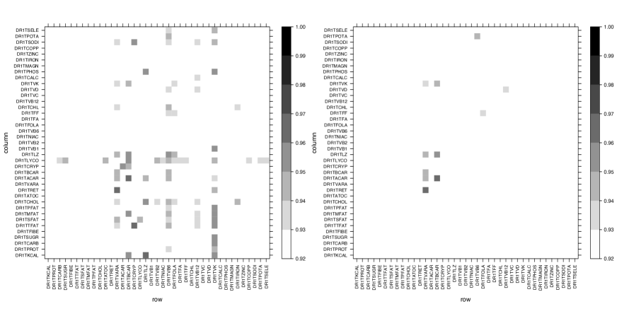
Figure 4: Matrices $\hat{\Delta}^{(2)}$ with entries $\hat{\sigma}_{\tilde{T}^{im}_{1},\tilde{T}^{im}_{2}}^{2}$ for all pairs $(i,m)$, where Algorithm 1 outputs $\hat{P}_{im}=1$ for $\varepsilon_{4}=0.01$ (left) and $\varepsilon_{4}=0.05$ (right).

The matrices $\hat{\Delta}^{(2)}$ in Figure 4 show non-zero entries of $\hat{\sigma}_{\tilde{T}^{im}_{1},\tilde{T}^{im}_{2}}^{2}$, where Algorithm 1 outputs $\hat{P}_{im}=1$. By Theorem 3.13 (a), for each non-zero entry $(i,m)$ we obtain the two-dimensional RMLM $(X_{i},X_{m})$ with edge $m\to i$. As we learnt from the simulation results for DAGs of dimension $D=40$ and $p=0.1$ in Appendix F, some of the estimated nodes in MWP correspond to false positives related only by confounders. The left-hand matrix $\hat{\Delta}^{(2)}$ reveals a large number of estimated MWP pairs, but the dependence is rather weak in most cases. By Remark 3.17, asymptotic independence implies $\Delta^{(2)}_{im}=\Delta^{(2)}_{mi}$, so to further filter out weakly dependent pairs, we take $\varepsilon_{4}=0.05$ for the error term. This leads to a lower number of estimated pairs of nodes in MWP, as shown by the right-hand panel of Figure 4.

The matrix $\hat{\Delta}^{(2)}$ depicted on the right-hand side of Figure 4 has non-zero entries only for the following twelve nutrients with abbreviations: AC = DR1TACAR (Alpha-Carotene), BC = DR1TBCAR (Beta-Carotene), VA = DR1TVARA (Vitamin A), LZ = DR1TLZ (Lutein+ Zeaxanthin), VK = DR1TVK (Vitamin K), VB12 = DR1TVB12 (Vitamin B12), FF=DR1TFF (Food Folate), FA=DR1TFA (Folic Acid), P=DR1TP (Potasium), VB6= DR1TVB6 (Vitamin B6), VD= DR1TVD (Vitamin D), and VB12= DR1TVB12 (Vitamin B12).

The first four were selected in Klüppelberg and Krali (2021). Compared to that paper, our new algorithm allows us to construct a larger DAG, composed of six of the 39 observed nutrients.

We have also now identified other two-dimensional RMLMs, for instance FF $\to$ FA, P $\to$ VB6, and VD $\to$ VB12. However, we are unable to establish connections between these separate DAGs due to the asymptotic dependence between the source nodes of the respective bivariate DAGs. Here this dependence indicates the possibility of confounders, analogous to the DAG $\mathcal{D}_{2}$ in Figure 1, but with an unknown number of hidden confounders.

A closer inspection shows that the pair (LZ,VK) does not belong to any set from $S_{1}$ to $S_{4}$, but exhibits very strong extreme dependence and symmetry, with $\sigma_{M_{im}}^{2}=1.19$. For this pair the given $\varepsilon^{\prime}$s seem too small, but larger values result in a large number of false positives. In this particular case, we draw the undirected red edge, to represent their indistinguishability.

From the matrix $\hat{P}$ and based on pairs in MWP only, we construct the DAG depicted in the right-hand panel of Figure 5, in which we draw directed edges between the nutrients $(i,m)$ for non-zero entries $\hat{P}_{im}$ of the matrix $\hat{P}$. We recall by Theorem 2.3 (i) that, in order to behave as source nodes, RET, AC, and LZ must be asymptotically independent, and in all cases we estimate $\hat{\sigma}_{M_{im}}^{2}\approx 1.9$ for $i,m\in\{{\rm RET,AC,LZ\}}$, with $\sigma_{M_{im}}^{2}=2$ corresponding to asymptotically independent extremes. A similar level of weak extreme dependence also occurs between the pairs (AC, VK), (RET, BC), (RET, VK), which helps to verify the conditions (3.13) of Theorem 2.3 and thus the feasibility of the RMLM.

Finally, the right-hand DAG in Figure 5 corresponds to the DAG $\mathcal{D}^{O}$ from Definition 2.1, generated from the minimal representation (2.2), and is obtained by drawing only the estimated max-weighted paths.

Figure 5: Left: DAG corresponding to $\hat{\Delta}^{(2)}$ as estimated in Figure 4 (right) with pairwise estimated directed edges (blue), where $\hat{P}_{im}=1$. The red undirected edge corresponds to the undistinguishable pair (VK, LZ) with $\hat{P}_{im}=0,\hat{P}^{*}_{im}=1$. Right: DAG  with only max-weighted paths, corresponding to the DAG $\mathcal{D}^{O}$ from Definition 2.1.

5 Conclusions

We make the realistic assumption that not all nodes of an underlying RMLM supported on a DAG are observed, so the observed node variables may not form a RMLM. Despite this we have seen that it may be possible to disregard hidden nodes, and in particular hidden confounders, in regularly varying RMLMs; we have given necessary and sufficient conditions for this. A key aspect is the construction of a RMLM based on max-weighted paths between pairs of node variables by estimating scalings and extreme dependence measures between pairs of transformed observations. The estimators are shown to be consistent and asymptotically normally distributed. A new algorithm that outputs the pairs of nodes that can be modelled by reduced RMLMs is studied by simulation and then applied to nutrition intake data.

Appendix A Proofs of Sections 2 and 3

Proof of Theorem 2.3.

We use a proof via induction over the number of generations of the observed DAG.

Skipping the case of a trivial DAG with a single generation $V_{0}^{O}$, we initiate the induction by showing that for two observed generations, $V_{0}^{O},G_{1}^{O}$, the conditions in (i) are necessary and sufficient.

Regarding necessity, we notice that such a DAG would simply consist of a set of source nodes and their children, connected by at most a path of length 1. As such, using the construction principle of a RMLM on a DAG, the innovations entering the representation of any source node, say $\ell$, have a max-weighted path to ${\rm de}(\ell)$ only via $\ell$, and hence (i)(b) holds. Assertion (i)(a) holds trivially by definition of the source nodes, since they have no common ancestors.

Next, we show sufficiency of (i). Since the observed DAG has two generations, we use representation (2.2) for $i\in G_{1}^{O}$ and $\ell\in V_{0}^{O}$, yielding

$$X_{i} =\bigvee_{k\in{\rm An}^{O}(i)}\frac{a_{ik}}{a_{kk}}X_{k}\vee\bigvee_{k\in{\rm An}^{O^{c}}(i)}a_{ik}Z_{k},\quad i\in G_{1}^{O}$$

$$X_{\ell} =\bigvee_{k\in{\rm An}^{O^{c}}(\ell)}a_{\ell k}Z_{k}\eqqcolon\tilde{Z}_{\ell},\quad\ell\in V_{0}^{O}.$$ (A.1)

We show that an innovation $Z_{u}$ can appear only once on the right-hand side, namely either $u\in{\rm An}^{O^{c}}(i)$, or $u\in\textrm{an}(k)$ for some $k\in{\rm An}^{O}(i)$. By definition, the former occurs only when there are no max-weighted paths $u\rightsquigarrow\ell\rightsquigarrow i$, for $\ell\in V_{0}^{O}$, and thus, by $(i)(b)$ when $u\in{\rm an}(i)\setminus{\rm an}(\ell)$. Otherwise, there is a max-weighted path $u\rightsquigarrow\ell\rightsquigarrow i$, hence $u\notin{\rm An}^{O^{c}}(i)$. The case when $j\in O\cap{\rm de}(\ell)^{c}$ is clear, as ${\rm an}(\ell)\cap{\rm an}(j)\cap O^{c}=\emptyset$ and ${\rm an}(\ell)\cap O=\emptyset$. If $j\in V_{0}^{O}$, then by (i)(a) the innovations are independent.

We may proceed similarly with the other nodes in $G_{1}^{O}$ to obtain the first two generations. Namely, for all $\ell\in V_{0}^{O}$ and all $i\in{\rm an}(\ell)$ we can obtain representations similar to (A). As the observed graph has two generations, there cannot be a path between $i$ and $j$ for $i,j\in G_{1}^{O}$. Therefore, the representations in (A) suffices to show that we have obtained a RMLM on a DAG with two generations.

Next, using the inductive hypothesis, suppose that there are $o-1<d$ such nodes belonging to $p-1$ observed generations (${\cup}_{i\leq p-1}{G^{O}_{i}}$), and that we can construct a RMLM on a DAG composed of the nodes in ${\cup}_{i\leq p-1}{G^{O}_{i}}$ if and only if (i) and (ii) are satisfied. Now, suppose we observe an additional generation, say $G^{O}_{p}$, and without loss of generality assume $G^{O}_{p}$ consists of one node, say ${o_{p_{1}}}$. We first show the necessity of (ii). By Theorem 6.7 of Gissibl and Klüppelberg [2018] we may write

$$X_{o_{p_{1}}} =\bigvee_{j\in{\rm An}^{O}({o_{p_{1}}})}\frac{a_{{o_{p_{1}}}j}}{a_{jj}}X_{j}\vee\bigvee_{j\in{\rm An}^{O^{c}}({o_{p_{1}}})}a_{{o_{p_{1}}}j}Z_{j}.$$ (A.2)

As before, we need to ensure that the innovations of the hidden ancestors of node ${o_{p_{1}}}$ appearing in ${\rm An}^{O^{c}}({o_{p_{1}}})$ are exogenous. We do so by contradiction: suppose that the observed $o$ nodes are generated via a RMLM on a DAG, and that there exists some $u\in O^{c}\cap{\rm an}({o_{p_{1}}})\cap{\rm an}(j)$ for some $j\in{\cup}_{i\leq p-1}{G^{O}_{i}}$ such that neither (a) nor (b) of (ii) hold for the pair $({o_{p_{1}}},j)$. Then,

• for $j\in{\rm an}({o_{p_{1}}})$, no max-weighted paths from $u$ to ${o_{p_{1}}}$ pass through $j$;

• for every $k\in{\rm an}({o_{p_{1}}})\cap{\rm an}(j)\cap O$ there are no max-weighted paths from $u$ to both ${o_{p_{1}}}$ and $j$ passing through $k$.

(C1) ensures that $Z_{u}$ will enter $X_{o_{p_{1}}}$ either via some node in ${\rm An}^{O}({o_{p_{1}}})\setminus\{j\}$ or via the set ${\rm An}^{O^{c}}({o_{p_{1}}})$. In the latter case, $Z_{u}$ entering ${\rm An}^{O^{c}}({o_{p_{1}}})$ implies that the innovations involved in ${\rm An}^{O^{c}}({o_{p_{1}}})$ are not exogenous, as $u$ enters the representation of $j$ as well, either via ${\rm An}^{O}(j)$, or ${\rm An}^{O^{c}}(j)$. This contradicts the assumption that the observed DAG corresponds to a RMLM. If $Z_{u}$ enters the representation of $X_{o_{p_{1}}}$ via ${\rm An}^{O}({o_{p_{1}}})\setminus\{j\}$, then there exists some node $r\in{\rm An}^{O}({o_{p_{1}}})\setminus\{j\}$ such that $u\in O^{c}\cap{\rm an}(r)\cap{\rm an}(j)$. Note, however, by the induction hypothesis, that since the nodes in the first $p-1$ generations form a RMLM, and since $j,r\in{\cup}_{i\leq p-1}G^{O}_{i}$, it must be the case that either there is a max-weighted path $u\rightsquigarrow r\rightsquigarrow j\rightsquigarrow{o_{p_{1}}}$, or $u\rightsquigarrow j\rightsquigarrow r\rightsquigarrow{o_{p_{1}}}$, or that there exists some node $k\in{\rm an}(r)\cap{\rm an}(j)\cap O\cap{\rm de}(u)$ such that there are max-weighted paths from $k$ to both $r$ and $j$. The first two such paths contradict (C1). The third path would also imply that there is a max-weighted path from $k$ to both $j$ and ${o_{p_{1}}}$, hence contradicting (C2). Similarly, $u\in{\rm An}^{O^{c}}(j)\cap{\rm An}^{O^{c}}({o_{p_{1}}})$ contradicts the exogeneity of the innovations composing the two respective sets due to the presence of $Z_{u}$.

Under (C2) $Z_{u}$ would appear in $X_{j}$ via either ${\rm An}^{O}(j)$ or ${\rm An}^{O^{c}}(j)$, and in $X_{o_{p_{1}}}$ via either ${\rm An}^{O}({o_{p_{1}}})\setminus\{j\}$ or ${\rm An}^{O^{c}}({o_{p_{1}}})$. Clearly, $u$ appearing in ${\rm An}^{O^{c}}(j)\cap{\rm An}^{O^{c}}({o_{p_{1}}})$, or in ${\rm An}^{O}(j)\cap{\rm An}^{O^{c}}({o_{p_{1}}})$ poses a contradiction to the exogeneity of the innovations involved in ${\rm An}^{O^{c}}({o_{p_{1}}})$. Similarly, $u$ appearing in ${\rm An}^{O^{c}}(j)\cap{\rm An}^{O}({o_{p_{1}}})\setminus\{j\}$, would imply that there is a max-weighted path from $u$ to ${o_{p_{1}}}$ via $r\in{\rm An}^{O}({o_{p_{1}}})\setminus\{j\}$. But then $u\in{\rm an}(r)\cap{\rm an}(j)$, and since $j,r\in{\cup}_{i\leq p-1}G^{O}_{i}$, by the induction hypothesis there exists some $k$ such that there are max-weighted paths from $k\in{\rm an}(r)\cap{\rm an}(j)\cap O\cap{\rm de}(u)$ to both $j$ and $r$, and hence to both $j$ and ${o_{p_{1}}}$, a contradiction to (C2). Finally, $u$ appearing in ${\rm An}^{O}(j)\cap{\rm An}^{O}({o_{p_{1}}})\setminus\{j\}$ implies that there are max-weighted paths from from $u$ to $j$ passing through $r_{1}\in{\rm An}^{O}(j)$, and to ${o_{p_{1}}}$ passing through $r_{2}\in{\rm An}^{O}({o_{p_{1}}})\setminus\{j\}$. Since $r_{1},r_{2}\in{\cup}_{i\leq p-1}G^{O}_{i}$, and $u\in{\rm an}(r_{1})\cap{\rm an}(r_{2})$, by the induction hypothesis there exists some $m\in{\rm An}^{O}(r_{1})\cap{\rm An}^{O}(r_{2})$ such that there are max-weighted paths from $u$ to both $r_{1}$ and $r_{2}$, and hence also to $j$ and ${o_{p_{1}}}$, passing through $m$, again a contradiction.

A similar argument applies when $G^{O}_{p}$ has more than one node, by considering (C2) above for ${o_{p_{1}}},{o_{p_{2}}}\in G^{O}_{p}$ and using the fact that there can be no paths within generations. This shows the necessity of the condition (ii). Note that (i) is a special case of (ii) for $j\in V_{0}$.

It remains to show sufficiency when there are more than two generations. Again, by the induction hypothesis, suppose that (i) and (ii) suffice for a DAG with $p-1$ generations to be generated by a RMLM.

Let ${o_{p}}\in G^{O}_{p}$ and focus on the representation in (2.2). It suffices to show that any $u\in{\rm An}^{O^{c}}({o_{p}})$ does not appear in any of the ancestral nodes of ${o_{p}}$ on the DAG in $O$. We may immediately rule out the nodes in $V_{0}$ by (i) as we would then run into a contradiction. For any remaining node $j$ we have three mutually exclusive possibilities, namely

• $j\in{\rm an}({o_{p}})\cap O$;

• there exists $q\in{\rm an}(j)\cap{\rm an}({o_{p}})\cap O$ and $j\notin{\rm an}(o)$;

• ${\rm an}(j)\cap{\rm an}({o_{p}})\cap O=\emptyset$.

We may disregard (D3); if that were the case for all nodes $j$ then either ${o_{p}}\in V_{0}$, or ${o_{p}}$ is the only descendant for a source node, which again points us to (i). Thus, we focus on the first two points.

Under (D1), if $j\in{\rm an}({o_{p}})$, then by (ii)(a) all $u$ in ${\rm an}(j)\cap{\rm an}({o_{p}})\cap O^{c}$ will have a max-weighted path to ${o_{p}}$ via $j$, or to both $j$ and ${o_{p}}$ via some $k$ in ${\rm an}(i)\cap{\rm an}({o_{p}})\cap O$, which ensures that $u\notin{\rm An}^{O^{c}}({o_{p}})$.

Under (D2), by condition (ii)(b) for every $u$ in ${\rm an}(j)\cap{\rm an}({o_{p}})\cap O^{c}$ there exists some $k$ in ${\rm an}(j)\cap{\rm an}({o_{p}})\cap O$ such that there are max-weighted paths from $u$ to $j$ and ${o_{p}}$, respectively, passing through $k$. This ensures that $Z_{u}$ appears directly in the representations of $X_{j}$ and $X_{{o_{p}}}$ via ${\rm An}^{O}(j)$ and ${\rm An}^{O}({o_{p}})$, respectively. Therefore, all innovations in ${\rm An}^{O^{c}}({o_{p}})$ must be exogenous to the ${o_{p}}$-th node and not enter the representation of the preceding nodes. Thus, all $X_{o_{p}}$ for ${o_{p}}\in G^{O}_{p}$ can be represented as a max-linear function of some ancestral nodes and some exogenous innovations via representation (A.2), and so, by induction, $\boldsymbol{X}_{O}$ can be formulated as a RMLM. ∎

Proof of Theorem 3.21..

The proof of (a) closely follows that of Theorem 3.13. From (3.18) it holds that $a_{mk}\geq a_{ik}$ for $k\in{\rm An}(m)\setminus{\rm An}(O_{\kappa})$ with strict inequality $a_{mm}>a_{im}$, and likewise for $\boldsymbol{T}^{\kappa im}$ when $c\leq 1$. Hence $\boldsymbol{T}^{\kappa im}$ has spectral measure

$$H_{{\boldsymbol{T}^{\kappa im}}}(\cdot)=\sum_{k\in{\rm An}(m)\setminus{\rm An}(O_{\kappa})}\lVert\tilde{a}_{k}\rVert^{2}\delta_{\big{\{}\frac{{\tilde{a}_{k}}}{\lVert\tilde{a}_{k}\rVert}\big{\}}}(\cdot),$$

where $\tilde{a}_{k}=(a_{mk}-c_{1}a_{ik},a_{mk}+c_{2}a_{ik})^{\top},$ for $k\in{\rm An}(m)\setminus{\rm An}(O_{\kappa})$, and $\tilde{a}_{k}=(0,0)$ otherwise, in particular for $k\in{\rm An}(i)\setminus{\rm An}(m)$, and, due to Lemmas B.9 and B.10, also for $k\in O_{\kappa}$ . Since for $k\in({\rm An}(i)\cap{\rm An}(m))\setminus{\rm An}(O_{\kappa})\neq\emptyset$ there is a max-weighted path from $k$ to $i$ via $m$ if and only if ${a_{ik}}{a_{mm}}={a_{im}}{a_{mk}}$, then $a_{ik}=ba_{mk}$ for all such $k$, giving $\tilde{a}_{k}=((1-c_{1}b)a_{mk},(1+c_{2}b)a_{mk})$.

The squared scaling of ${T}^{\kappa im}_{3,2}$ equals $\sigma_{{T}^{\kappa im}_{3,2}}^{2}=\sum_{k\in{\rm An}(m)\setminus{\rm An}(O_{\kappa})}a_{mk}^{2}$, which implies that the scalings of ${T}^{\kappa im}_{1}$ and ${T}^{\kappa im}_{2}$ become $(1-c_{1}b)\sigma_{{T}^{\kappa im}_{3,2}}^{2}$ and $(1+c_{2}b)\sigma_{{T}^{\kappa im}_{3,2}}^{2}$. Upon standardizing the components $\boldsymbol{T}^{\kappa im}$ to unit scalings, say, into the vector $\boldsymbol{\tilde{T}}^{\kappa im}$, by arguments similar to those of the proof of Theorem 3.13, it is clear that $\sigma_{{\tilde{T}}^{\kappa im}_{1},{\tilde{T}}^{\kappa im}_{2}}^{2}=1$.

The reasoning in the other direction mimics the Cauchy–Schwarz inequality argument in the proof of Theorem 3.13, but with the index of the summation ranging in ${\rm An}(m)\setminus{\rm An}(O_{\kappa})$. Because $a_{mm}>0$ and ${\rm An}(i)\cap{\rm An}(m)\setminus{\rm An}(O_{\kappa})\neq\emptyset$, we must have $a_{im}>0$. The Cauchy–Schwarz equality would then imply that ${a_{ik}}{a_{mm}}={a_{im}}{a_{mk}}$ for $k\in({\rm An}(i)\cap{\rm An}(m))\setminus{\rm An}(O_{\kappa})$.

The proof of (b) is identical to that of Theorem 3.13; the only change is again in the index $k\in({\rm An}(i)\cap{\rm An}(m))\setminus{\rm An}(O_{\kappa})\neq\emptyset$. ∎

Appendix B Multivariate regular variation

B.1 Definitions and results for regularly varying vectors

We state two equivalent definitions of multivariate regular variation taken from Resnick [28], Theorem 6.1.

Definition B.1.

(a)   A random vector $\boldsymbol{Y}\in\mathbb{R}^{d}_{+}$ is multivariate regularly varying if there exists a sequence of real numbers $b_{n}\to\infty$ as $n\to\infty$ such that

$$n\mathbb{P}(\boldsymbol{Y}/{b_{n}}\in\cdot)\overset{v}{\to}{\nu_{\boldsymbol{X}}}(\cdot),\hskip 14.22636ptn\to\infty,$$ (B.1)

where $\overset{v}{\to}$ denotes vague convergence in $M_{+}(\mathbb{R}_{+}^{{d}}\setminus\{\boldsymbol{0}\})$, the set of non-negative Radon measures on $\mathbb{R}_{+}^{d}\setminus\{\boldsymbol{0}\}$, and $\nu_{\boldsymbol{Y}}$ is called the exponent measure of $\boldsymbol{Y}$.
(b)   A random vector $\boldsymbol{Y}\in\mathbb{R}^{{d}}_{+}$ is multivariate regularly varying if for any norm $\|\cdot\|$ there exists a finite measure $H_{\boldsymbol{Y}}$ on the positive unit sphere $\Theta_{+}^{{{d}}-1}=\{\boldsymbol{\omega}\in\mathbb{R}^{{d}}_{+}:\lVert\boldsymbol{\omega}\rVert=1\}$ and a sequence $b_{n}\to\infty$ as $n\to\infty$ such the angular representation $(R,\boldsymbol{\omega})\coloneqq(\lVert\boldsymbol{Y}\rVert,\boldsymbol{Y}/\lVert\boldsymbol{Y}\rVert)$ of $\boldsymbol{Y}$ satisfies

$$n\mathbb{P}\left(\left({R}/{b_{n}},\boldsymbol{\omega}\right)\in\cdot\right)\overset{v}{\to}\nu_{\alpha}\times H_{\boldsymbol{Y}}(\cdot),\hskip 14.22636ptn\to\infty,$$ (B.2)

in $M_{+}((0,\infty]\times\Theta_{+}^{{{d}}-1})$, ${\rm d}\nu_{\alpha}(x)=\alpha x^{-\alpha-1}{\rm d}x$ for some $\alpha>0$, and for Borel subsets $C\subseteq\Theta_{+}^{{{d}}-1}$,

$$H_{\boldsymbol{Y}}(C)\coloneqq\nu_{\boldsymbol{Y}}\big{(}\{\boldsymbol{y}\in\mathbb{R}^{{d}}_{+}\setminus\{\boldsymbol{0}\}:\lVert\boldsymbol{y}\rVert\geq 1,\boldsymbol{y}/\lVert\boldsymbol{y}\rVert\in{C}\}\big{)}.$$

In this case the measure $H_{\boldsymbol{Y}}$ is called the spectral measure of $\boldsymbol{Y}$, we write $\boldsymbol{Y}\in{\rm RV}^{{d}}_{+}(\alpha)$, and call $\alpha$ the index of regular variation.   $\Box$

We will use the following equivalent representation of multivariate regular variation of a vector $\boldsymbol{Y}$ with standardized margins.

Proposition B.2.

Let $\boldsymbol{Y}\in\mathbb{R}^{d}_{+}$ have standardized margins such that $\mathbb{P}(Y_{i}>y)\sim y^{-\alpha}$ as $y\to\infty$ for $i\in\{1,\ldots,d\}$ and $\alpha>0$. Assume further that $R=\lVert\boldsymbol{Y}\rVert\in{\rm RV}_{+}(\alpha)$ such that $\mathbb{P}(R>r)\sim d^{1/\alpha}r^{-\alpha}$ as $r\to\infty$, and that for $\boldsymbol{\omega}=\boldsymbol{Y}/\lVert\boldsymbol{Y}\rVert\in{\Theta}^{d-1}_{+}$, and constants $b_{n}\sim(dn)^{1/\alpha}$,

$$\mathbb{P}\left(\boldsymbol{\omega}\in\cdot\,|\,R/b_{n}>1\right)\overset{w}{\to}\tilde{H}_{\boldsymbol{Y}}(\cdot),\quad n\to\infty,$$ (B.3)

where $\overset{w}{\to}$ denotes weak convergence and $\tilde{H}_{\boldsymbol{Y}}$ is a probability measure on ${\Theta}^{d-1}_{+}$. Then $\boldsymbol{Y}\in{\rm RV}^{{d}}_{+}(\alpha)$.

Proof.

We prove the equivalence to Definition B.1 (b). Without loss of generality we focus on the case $\alpha\geq 1$, and choose $\lVert\cdot\rVert_{\alpha}$ as choice of norm. Vectors which are multivariate regularly varying with $\alpha<1$ can always be transformed to a regular variation index greater than 1.

Since $\{[r,\infty),r>0\}$ generate the Borel sets in $(0,\infty]$, Definition B.1 (b) is equivalent to

$${n}\mathbb{P}\left(R/{b^{\prime}_{n}}>r,\boldsymbol{\omega}\in\cdot\right)\overset{w}{\to}\nu_{\alpha}\left([r,\infty)\right)\times H_{\boldsymbol{Y}}(\cdot),\hskip 14.22636ptn\to\infty,$$ (B.4)

for $r>0$, the measure ${H}_{\boldsymbol{Y}}$ on $\Theta_{+}^{{{d}}-1}$, and the normalizing constants $b^{\prime}_{n}$, say, to distinguish $b_{n}$ in (B.3).

We first show that (B.4) implies regular variation of $R$ and (B.3). Indeed, we obtain

$${n}\mathbb{P}\left(R/{b^{\prime}_{n}}>r\right)={n}\mathbb{P}\left(R/{b^{\prime}_{n}}>r,\boldsymbol{\omega}\in\Theta^{d-1}_{+}\right)\to r^{-\alpha}\times H_{\boldsymbol{Y}}(\Theta^{d-1}_{+}),\quad n\to\infty.$$

To select appropriate constants $b_{n}$, we first adjust for the mass ${H}_{\boldsymbol{Y}}(\Theta_{+}^{{{d}}-1})$ which, in a similar fashion to Cooley and Thibaud [2019, p. 592], can be computed using Definition B.1 (b) as follows:

$$H_{\boldsymbol{Y}}(\Theta_{+}^{{{d}}-1}) =\int_{\Theta_{+}^{{{d}}-1}}\lVert\boldsymbol{\omega}\rVert^{\alpha}{\rm d}H_{{\boldsymbol{Y}}}(\boldsymbol{\omega})$$

$$=\int_{\Theta_{+}^{{{d}}-1}}\sum_{j=1}^{d}\omega_{j}^{\alpha}{\rm d}H_{{\boldsymbol{Y}}}(\boldsymbol{\omega})=\sum_{j=1}^{d}\int_{\Theta_{+}^{{{d}}-1}}\omega_{j}^{\alpha}{\rm d}H_{{\boldsymbol{Y}}}(\boldsymbol{\omega})$$

$$=\sum_{j=1}^{d}\int_{\Theta_{+}^{{{d}}-1}}\int_{r>\omega_{j}^{-1}}\alpha r^{-(\alpha+1)}{\rm d}r{\rm d}H_{{\boldsymbol{Y}}}(\boldsymbol{\omega})$$

$$=\sum_{j=1}^{d}\lim_{n\to\infty}n\mathbb{P}\left(R/{b^{\prime}_{n}}>\omega_{j}^{-1},\boldsymbol{\omega}\in\Theta_{+}^{{{d}}-1}\right)$$

$$=\sum_{j=1}^{d}\lim_{n\to\infty}n\mathbb{P}\left(Y_{j}/{b^{\prime}_{n}}>1\right)=d,$$ (B.5)

where we have used (B.4) and the fact that $R\omega_{j}=Y_{j}$ and $b^{\prime}_{n}\sim n^{1/\alpha}$ are correct normalizing constants for $Y_{j}$. Therefore, to normalize the mass of $H_{{\boldsymbol{Y}}}$, without loss of generality, we can fix constants $b_{n}$ for $R$ such that $b_{n}\sim(dn)^{1/\alpha}$ as $n\to\infty$. Using the latter constant, and setting $r=1$ in (B.2) immediately leads to (B.3) with the normalized spectral measure $\tilde{H}_{{\boldsymbol{Y}}}$. Hence, (B.2) implies regular variation of $R$ and (B.3).

Now, we want to show that Proposition B.2 implies (B.2). Using that $\mathbb{P}(R>r)\sim d^{1/\alpha}r^{-\alpha}$ and the constants $b_{n}\sim(dn)^{1/\alpha}$, we re-write (B.4) as

$${n}\mathbb{P}\left(R/{b_{n}}>r,\boldsymbol{\omega}\in\cdot\right) \sim r^{-\alpha}{nr^{\alpha}}\mathbb{P}\left(R/{b_{nr^{\alpha}}}>1,\boldsymbol{\omega}\in\cdot\right)$$

$$=r^{-\alpha}\mathbb{P}\left(R/{b_{nr^{\alpha}}}>1,\boldsymbol{\omega}\in\cdot\,|\,R/b_{nr^{\alpha}}>1\right)$$

$$=r^{-\alpha}\mathbb{P}\left(\boldsymbol{\omega}\in\cdot\,|\,R/b_{nr^{\alpha}}>1\right)$$

$$\overset{w}{\to}\nu_{\alpha}\left([r,\infty)\right)\times\tilde{H}_{\boldsymbol{X}}(\cdot),\quad n\to\infty,$$ (B.6)

where $\tilde{H}_{\boldsymbol{X}}(\cdot)={H}_{\boldsymbol{X}}(\cdot)/d$, since the mass $d$ is now absorbed into the normalizing sequence $b_{n}$. The last convergence is due to (B.3). Hence, we have proved (B.4), which is equivalent to (B.2) for the choice of constants $b_{n}$. ∎

B.2 Regularly varying RMLMs

Proposition B.3.

([Krali, 2018, Proposition 4.1])
Let $\boldsymbol{Z}\in{\rm RV}^{D}_{+}(\alpha)$ with independent components $Z_{k}\in{\rm RV}_{+}(\alpha)$, $A\in{\mathbb{R}}_{+}^{d\times D}$ and

$$\boldsymbol{X}=A\times_{\max}\boldsymbol{Z}.$$ (B.7)

Then $\boldsymbol{X}\in{\rm RV}^{d}_{+}(\alpha)$ with discrete spectral measure

$$H_{\boldsymbol{X}}(\cdot)=\sum_{k=1}^{D}\lVert a_{k}\rVert^{\alpha}\delta_{\big{\{}\frac{{a_{k}}}{\lVert a_{k}\rVert}\big{\}}}(\cdot),$$ (B.8)

on the positive unit sphere $\Theta_{+}^{d-1}$ with atoms $(a_{k}/\lVert a_{k}\rVert)_{k=1,\dots,D}$ for $a_{k}=(a_{1k},\dots,a_{dk})$; i.e. the atoms are the normalized $k$-th columns of $A$. The finite measure $H_{\boldsymbol{X}}$ can be normalized to a probability measure by defining

$$\tilde{H}_{\boldsymbol{X}}(\cdot)\coloneqq\frac{H_{\boldsymbol{X}}(\cdot)}{H_{\boldsymbol{X}}(\Theta_{+}^{{d}-1})}.$$ (B.9)

Corollary B.4.

(a)([Gissibl et al., 2018, Proposition A.2]) For a set $[\boldsymbol{0},\boldsymbol{x}]^{c}$ the exponent measure is given by

$$\nu_{\boldsymbol{X}}([\boldsymbol{0},\boldsymbol{x}]^{c})=\sum_{k=1}^{D}\underset{i=1}{\overset{d}{\bigvee}}\frac{a_{ik}^{\alpha}}{x_{i}^{\alpha}}.$$

(b) Let $a_{ik}=a_{jk}$ for all $k\in\{1,\dots,D\}$ as in Corollary 3.4(c). Then

$$\nu_{\boldsymbol{X}}([\boldsymbol{0},\boldsymbol{x}]^{c})=\sum_{k=1}^{D}a_{1k}^{\alpha}\underset{i=1}{\overset{d}{\bigvee}}x_{i}^{-\alpha}=\sum_{k=1}^{D}a_{1k}^{\alpha}\,\Big{(}\underset{i=1}{\overset{d}{\bigwedge}}x_{i}\Big{)}^{-\alpha},$$

giving asymptotically full dependence by Resnick [2007, eq. (6.32)].

We denote the set of random vectors $\boldsymbol{X}$ as in (B.7) by ${\rm RV}^{d}_{+}(\alpha,A)$ and denote the rows of $A$ by $A_{i}$ for $i\in\{1,\dots,d\}$. Let now $\boldsymbol{X}\in{\rm RV}^{d}_{+}(\alpha,A)$, then each component of $\boldsymbol{X}$ has representation

$$X_{i}=A_{i}\times_{\max}\boldsymbol{Z}=\bigvee_{k\in\{1,\dots,D\}}a_{ik}Z_{k},\quad i\in\{1,\dots,d\}.$$

This motivates the following.

Proposition B.5.

Consider the set of random variables

$$\{X=a\times_{\max}\boldsymbol{Z}\in{\rm RV}_{+}(\alpha,a):a\in{\mathbb{R}}^{D}_{+}\}.$$

This set has the following properties:

1. For $c>0$ and $X\in{\rm RV}_{+}(\alpha,a)$ we have $cX\in{\rm RV}_{+}(\alpha,ca)$.

2. Let $X_{1}\in{\rm RV}_{+}(\alpha,a_{1})$ and $X_{2}\in{\rm RV}_{+}(\alpha,a_{2})$, then $(X_{1},X_{2})\in{\rm RV}^{2}_{+}(\alpha,A_{12})$ with $A_{12}=(a_{1},a_{2})^{\top}$; i.e. $(X_{1},X_{2})$ has discrete spectral measure with atoms given by the normalized non-zero columns of $A_{12}$.

3. Let $X_{1}\in{\rm RV}_{+}(\alpha,a_{1})$ and $X_{2}\in{\rm RV}_{+}(\alpha,a_{2})$, then $\max\{X_{1},X_{2}\}\in{\rm RV}_{+}(\alpha,a_{1}\vee a_{2})$, where $a_{1}\vee a_{2}$ is taken componentwise.

Proof.

(a) follows directly from the representation of $X$.
(b) is a simple consequence of considering the vector $(X_{1},X_{2})$, therefore arranging the transposed vectors $a_{1},a_{2}$ into rows of a new matrix $A_{12}\in\mathbb{R}_{+}^{2\times D}$. The atoms are then derived from Proposition B.3.
(c) is a consequence of max-linearity:

$$X_{1}\vee X_{2}=\underset{j\in\{1,2\}}{\vee}\underset{k\in\{1,\ldots,D\}}{\vee}a_{jk}Z_{k}=\underset{k\in\{1,\ldots,D\}}{\vee}(\underset{j\in\{1,2\}}{\vee}a_{jk})Z_{k}.$$

∎

From this we can immediately read off the first two lines of Table 3.1 and also of Table 3.2. For the third lines in Tables 3.1 and 3.2, we use the following multivariate version of Breiman’s lemma in combination with Proposition B.5.

Lemma B.6.

[Basrak et al. [2002, Proposition A.1]] Let $\boldsymbol{Y}\in{\rm RV}^{d}(\alpha)$, and $S$ be a random $q\times d$ matrix, independent of $\boldsymbol{Y}$. If $0<\mathbb{E}\lVert S\rVert^{\gamma}<\infty$ for some $\gamma>\alpha$ then

$$n\mathbb{P}(b_{n}^{-1}S\boldsymbol{Y}\in\cdot)\overset{v}{\to}\tilde{\nu}(\cdot)\coloneqq\mathbb{E}[\nu\circ S^{-1}(\cdot)],$$

where $\overset{v}{\to}$ denotes vague convergence on ${\mathbb{R}}^{d}\setminus\{0\}$.

Corollary B.7.

Let $\boldsymbol{X}=A\times_{\max}\boldsymbol{Z}$ be as in Proposition B.5, such that the normalized non-zero column vectors of the $d\times D$-matrix $A$ are the atoms of the spectral measure of $\boldsymbol{X}$ on the positive unit sphere. Let $S\in{\mathbb{R}}^{q\times d}$ be a non-random matrix. Then the linear transformation $S\boldsymbol{X}=S(A\times_{\max}\boldsymbol{Z})\in{\rm RV}^{d}(\alpha)$ has discrete spectral measure on the unit sphere $\Theta^{d-1}=\{\omega\in{\mathbb{R}}^{d}:\|\omega\|=1\}$ with atoms given by the normalized non-zero columns of $SA$.

Lemma B.8.

Let $\boldsymbol{X}\in{\rm RV}_{+}^{d}(\alpha,A)$ with $A\in\mathbb{R}_{+}^{d\times D}$. Recall $\boldsymbol{T}_{2}^{im}=(M_{c_{1}im},M_{im},X_{i},X_{m})$ from Table 3.1 and define the matrix

$$S=\begin{bmatrix}1&0&-c_{1}&0\\ 0&-c_{2}&c_{2}&1+c_{2}\\ \end{bmatrix}\in\mathbb{R}^{2\times 4}.$$

Then $\boldsymbol{T}^{im}:=S\boldsymbol{T}_{2}^{im}=(M_{c_{1}i,m}-c_{1}X_{i},(1+c_{2})X_{m}+c_{2}X_{i}-c_{2}M_{im})$, $\boldsymbol{T}^{im}\in{\rm RV}^{2}(\alpha)$ and has discrete spectral measure with non-normalized and non-zero atoms $\tilde{a}_{k}=(c_{1}a_{ik}\vee a_{mk}-c_{1}a_{ik},(1+c_{2})a_{mk}+c_{2}a_{ik}-c_{2}(a_{ik}\vee a_{mk}))$.

Proof.

From Proposition B.5 we read off the non-zero atoms $(\tilde{a}_{k}/\lVert\tilde{a}_{k}\rVert)$ of the spectral measure of $\boldsymbol{T}_{2}^{im}$ where $\tilde{a}_{k}=(c_{1}a_{ik}\vee a_{mk},a_{ik}\vee a_{mk},a_{ik},a_{mk})$. Applying Corollary B.7, the result follows. ∎

Lemma B.9.

Let $\boldsymbol{X}\in{\rm RV}_{+}^{d}(\alpha,A)$ be a $d-$dimensional subvector of a RMLM with ML coefficient matrix $A\in\mathbb{R}_{+}^{d\times D}$. Recall $\boldsymbol{T}_{2}^{\kappa im}\coloneqq(M_{O_{\kappa}},M_{O_{\kappa},i},M_{O_{\kappa},m})$ from Table 3.2 and define the matrix

$$S=\begin{bmatrix}-1&1&0\\ -1&0&1\\ \end{bmatrix}\in\mathbb{R}^{2\times 3}.$$

Then $\boldsymbol{T}^{\kappa im}_{3}\coloneqq(M_{O_{\kappa},i}-M_{O_{\kappa}},M_{O_{\kappa},m}-M_{O_{\kappa}})=S\boldsymbol{T}_{2}^{\kappa im}$, $\boldsymbol{T}^{\kappa im}_{3}\in{\rm RV}^{2}(\alpha)$ and has discrete spectral measure with non-normalized and non-zero atoms $\tilde{a}_{k}=(\underset{j\in O_{\kappa}\cup\{i\}}{\vee}a_{jk}-\underset{j\in O_{\kappa}}{\vee}a_{jk},\underset{j\in O_{\kappa}\cup\{m\}}{\vee}a_{mk}-\underset{j\in O_{\kappa}}{\vee}a_{jk})=(a_{ik}\mathds{1}_{\{k\notin{\rm An}(O_{\kappa})\}},a_{mk}\mathds{1}_{\{k\notin{\rm An}(O_{\kappa})\}}).$

Proof.

From Proposition B.5 we read off the atoms of the spectral measure of ${\boldsymbol{T}_{2}^{\kappa im}}$ by normalizing the non-zero vectors $(\underset{j\in O_{\kappa}\cup\{i\}}{\vee}a_{jk},\underset{j\in O_{\kappa}}{\vee}a_{jk},\underset{j\in O_{\kappa}\cup\{m\}}{\vee}a_{mk},\underset{j\in O_{\kappa}}{\vee}a_{jk})$. Applying Corollary B.7, the first representation of $\tilde{a}_{k}$ follows. The second representation is due to the causal ordering of the nodes in $O_{\kappa}$ and Lemma 3.5, since both $a_{ij},a_{mj}$ are strictly less than $a_{kj}$ for some $k\in O_{\kappa}$. This results in

$$\underset{j\in O_{\kappa}\cup\{i\}}{\vee}a_{jk}=\begin{cases}\underset{j\in O_{\kappa}}{\vee}a_{jk},&k\in{\rm An}(O_{\kappa}),\\ a_{ik},&k\notin{\rm An}(O_{\kappa}),\end{cases}$$

and likewise for $a_{m}$. ∎

Lemma B.10.

Let $\boldsymbol{X}\in{\rm RV}_{+}^{d}(\alpha,A)$ satisfy the setting of Lemma B.9. Set $\boldsymbol{T}_{4}^{\kappa im}\coloneqq(M^{\kappa}_{c_{1}i,m},M^{\kappa}_{i,m},$ ${T}_{3,1}^{\kappa im},{T}_{3,2}^{\kappa im})$, for components defined around (3.17), and define the matrix

$$S=\begin{bmatrix}1&0&-c_{1}&0\\ 0&-c_{2}&c_{2}&1+c_{2}\\ \end{bmatrix}\in\mathbb{R}^{2\times 4}.$$

Recall $\boldsymbol{T}^{\kappa im}\coloneqq(M^{\kappa}_{c_{1}i,m}-c_{1}{T}^{\kappa im}_{31},(1+c_{2}){T}^{\kappa im}_{32}+c_{2}{T}^{\kappa im}_{31}-c_{2}M^{\kappa}_{im})$ from (3.17). Then $\boldsymbol{T}^{\kappa im}=S\boldsymbol{T}^{\kappa im}_{4}$, $\boldsymbol{T}^{\kappa im}\in{\rm RV}^{2}(\alpha)$ and has discrete spectral measure with non-normalized non-zero atoms $\tilde{a}_{k}=(c_{1}a_{ik}\vee a_{mk}-c_{1}a_{ik},(1+c_{2})a_{mk}+c_{2}a_{ik}-c_{2}(a_{ik}\vee a_{mk}))\mathds{1}_{\{k\notin{\rm An}(O_{\kappa})\}}.$

Proof.

The proof follows by applying Lemmas B.8 and B.9 to the vector $\boldsymbol{T}^{\kappa im}_{3}$, instead of $(X_{i},X_{m})$. ∎

Appendix C Statistical theory for regularly varying innovations

We start with some notation and results from Resnick [2007], as in Section 6 of Klüppelberg and Krali [2021].

Let $\boldsymbol{Y}_{1},\ldots,{\boldsymbol{Y}_{n}}$ for $n\in{\mathbb{N}}$ be independent replicates of $\boldsymbol{Y}\in{\rm RV}^{d}_{+}(\alpha)$ with standardized margins, and consider the angular decomposition of $\boldsymbol{Y}$ given by

$$R\coloneqq\lVert\boldsymbol{Y}\rVert,\quad\boldsymbol{\omega}=(\omega_{1},\ldots,\omega_{d})=\frac{\boldsymbol{Y}}{R}.$$ (C.1)

We call $R$ the radial and $\boldsymbol{\omega}$ the angular component. Similarly for $\boldsymbol{Y}_{\ell}$ we write $R_{\ell}=\|\boldsymbol{Y}_{\ell}\|$ and $\boldsymbol{\omega_{\ell}}=\boldsymbol{Y}_{\ell}/R_{\ell}$ for $\ell\in\{1,\ldots,n\}$.

The standardized spectral measure $\tilde{H}_{\boldsymbol{Y}}$ from (B.9) provides a way to obtain a consistent estimator from the empirical spectral measure [see, e.g., (9.32) of Resnick, 2007], given for known normalizing functions $b_{n/k}$ by

$$\tilde{H}_{\boldsymbol{Y},n/k}(\cdot)=\frac{\sum_{\ell=1}^{n}\mathds{1}{\{(R_{\ell}/b_{\frac{n}{k}},{\boldsymbol{\omega}}_{\ell})\in[1,\infty]\times\cdot\}}}{\sum_{\ell=1}^{n}\mathds{1}{\{R_{\ell}/b_{\frac{n}{k}}\geq 1\}}}\stackrel{{\scriptstyle w}}{{\rightarrow}}\tilde{H}_{\boldsymbol{Y}}(\cdot),$$ (C.2)

as $n\to\infty$, $k\to\infty$, $k/n\to 0$.

Let $R^{(n)}\leq\cdots\leq R^{(1)}$ denote the order statistics of $R_{1},\ldots,R_{n}$. If we choose normalizing functions $b_{t}$ such that

$$t{\bf{\mathbb{P}}}(\boldsymbol{Y}/b_{t}\in\cdot) \stackrel{{\scriptstyle v}}{{\rightarrow}} \nu_{\boldsymbol{Y}}(\cdot),\quad t\to\infty,$$ (C.3)

then from Resnick [2007, p. 308], we know that $R^{(k)}/b_{n/k}\overset{P}{\to}1$, which suggests setting $b_{n/k}=R^{(k)}$ in (C.2) and gives the estimator

$$\tilde{H}_{\boldsymbol{Y},n/k}(\cdot)=\frac{1}{k}\sum_{\ell=1}^{n}\mathds{1}\{R_{\ell}\geq R^{(k)},\boldsymbol{\omega}_{\ell}\in\cdot\},$$ (C.4)

where $k=\sum_{\ell=1}^{n}\mathds{1}\{R_{\ell}\geq R^{(k)}\}$.

Our goal is to estimate extreme dependence measures and squared scalings as in Definition 3.1, and we define for a continuous function $f:\Theta^{d}_{+}\to{\mathbb{R}}_{+}$ the quantity

$${\mathbb{E}}_{\tilde{{H}}_{\boldsymbol{Y}}}[f(\boldsymbol{\omega})]:=\lim_{x\to\infty}{\mathbb{E}}[f(\boldsymbol{\omega})\mid R>x]=\int_{\Theta^{d}_{+}}f(\boldsymbol{\omega})d\tilde{H}_{\boldsymbol{Y}}(\boldsymbol{\omega}).$$

Thus a natural estimator for $\mathbb{E}_{\tilde{{H}}_{\boldsymbol{Y}}}[f(\boldsymbol{\omega})]$ is eq. (29) of Klüppelberg and Krali [2021], given by

$$\hat{\mathbb{E}}_{\tilde{{H}}_{\boldsymbol{Y}}}[f(\boldsymbol{\omega})]=\frac{1}{k}\sum_{\ell=1}^{n}f(\boldsymbol{\omega}_{\ell})\mathds{1}\{R_{\ell}\geq R^{(k)}\}.$$ (C.5)

The function $f(\cdot)$ will depend on whether we want to estimate extreme dependence measures or squared scalings.

C.1 Intermediate thresholding

Klüppelberg and Krali [2021] use the setting from the previous section to estimate squared scalings of partial maxima of selected components of a RMLM in their Section 6. In the present paper we want to estimate the extreme dependence measure of the components of $\boldsymbol{\tilde{T}}^{im}=(\tilde{T}_{1}^{im},\tilde{T}_{2}^{im})$ as defined in Section 3.3. The transformation of the sample variables to $\boldsymbol{\tilde{T}}^{im}$ creates many small values near $\boldsymbol{0}$, corrupting the estimator (C.5) significantly. As a remedy, we have implemented a two-step procedure using besides $k$ as in (C.5) an additional intermediate threshold.

For a given large sample $\boldsymbol{Y}_{1},\ldots,\boldsymbol{Y}_{n}$ in ${\rm RV}^{d}_{+}(\alpha)$ with standardised margins and with angular decompositon  (C.1) we choose a threshold $k_{1}$. Consider for $\ell\in\{1,\dots,n\}$ only those observations whose radial components satisfy $R_{\ell}\geq b_{n/{k_{1}}}$ for normalizing constants $b_{n/{k_{1}}}$ as in (C.2), and define

$$N_{n}=\sum_{\ell=1}^{n}\mathds{1}\{R_{\ell}\geq b_{n/{k_{1}}}\}.$$ (C.6)

Following the découpage de Lévy [Resnick, 2007, p. 15], these observations are also independent and identically distributed. Assume that $k_{1}=k_{1}(n)\to\infty$ and $k_{1}/n\to 0$ as $n\to\infty$, and choose normalizing constants $b_{n/k_{1}}\sim(dn/k_{1})^{1/\alpha}$. Here $d$ corresponds to the total mass of the spectral measure $H_{\boldsymbol{Y}}$ from Definition B.1(b), and including it in the normalizing constant leads to the normalisation of the spectral measure as shown in (B.1) in Appendix B.1. By definition, $\frac{1}{n}N_{n}$ is the empirical estimator of ${\bf{\mathbb{P}}}(R\geq b_{n/k_{1}})\sim db_{n/k_{1}}^{-\alpha}\sim k_{1}/n$ giving

$$\frac{1}{k_{1}}N_{n} \stackrel{{\scriptstyle P}}{{\rightarrow}} 1,\quad n\to\infty.$$ (C.7)

Assume that as $n\to\infty$, $k_{1}=k_{1}(n)\to\infty$, and select a sequence $k_{2}=k_{2}(k_{1})\to\infty$ such that $k_{2}/k_{1}\to 0$. We modify the estimator (C.5) by first disregarding all small observations and only take the $N_{n}$ observations with radial component larger than $b_{n/k_{1}}$ into account. For fixed $k_{1}$ define conditional random vectors

$$\tilde{\boldsymbol{Y}}_{\ell}=d^{1/\alpha}\boldsymbol{Y}_{\ell}/b_{n/k_{1}}\mid R_{\ell}\geq b_{n/k_{1}},\quad\ell\in\{1,\dots,N_{n}\}.$$ (C.8)

Lemma C.1.

Let $\boldsymbol{Y}\in{\rm RV}_{+}^{d}(\alpha)$ with angular decomposition (C.1). Assume that as $n\to\infty$, $k_{1}=k_{1}(n)\to\infty$, and select a sequence $k_{2}=k_{2}(k_{1})\to\infty$ such that $k_{2}/k_{1}\to 0$. Choose the normalizing constants $b_{{n}/{k_{i}}}$ such that for $i=1,2,$

$$\mathbb{P}(R\geq b_{{n}/{k_{i}}})\sim{\frac{k_{i}}{n}.}$$

Consider the conditional random vectors as in (C.8). Then $\tilde{\boldsymbol{Y}}\in{\rm RV}_{+}^{d}(\alpha)$ with angular decomposition $(\tilde{\boldsymbol{Y}}/\tilde{R},\tilde{R})$ satisfying

$$\mathbb{P}(\frac{\tilde{\boldsymbol{Y}}}{\tilde{R}}\in\cdot\mid\tilde{R}\geq b_{k_{1}/k_{2}}) \overset{w}{\to}\tilde{H}_{\boldsymbol{Y}}(\cdot),\quad n\to\infty$$ (C.9)

for $b_{k_{1}/k_{2}}$ such that ${\bf{\mathbb{P}}}(\tilde{R}\geq b_{k_{1}/k_{2}})\sim{k_{2}/k_{1}}$, and where $\tilde{H}_{\boldsymbol{Y}}$ is a probability measure on ${\Theta}^{d-1}_{+}$.

Proof.

Note first that by (B.1) the choice of the normalizing constants is correct for $\boldsymbol{Y}$. From (C.8) we obtain $\tilde{R}=\lVert\tilde{\boldsymbol{Y}}\rVert$. The following exploits Proposition (B.2). Choose normalizing constants $b_{k_{1}/k_{2}}\sim(dk_{1}/k_{2})^{1/\alpha}$ and note that $d^{-1/\alpha}b_{n/k_{1}}b_{k_{1}/k_{2}}\sim(n/k_{1})^{1/\alpha}(dk_{1}/k_{2})^{1/\alpha}=(dn/k_{2})^{1/\alpha}\sim b_{n/k_{2}}$. Then for the conditional radial component we find

$$\mathbb{P}(\tilde{R}>b_{k_{1}/k_{2}}) =\mathbb{P}(d^{1/\alpha}R/b_{n/k_{1}}>b_{k_{1}/k_{2}}\mid R\geq b_{n/k_{1}})=\frac{\mathbb{P}(R>d^{-1/\alpha}b_{n/k_{1}}b_{k_{1}/k_{2}},R\geq b_{n/k_{1}})}{\mathbb{P}(R\geq b_{n/k_{1}})}$$

$$\sim\frac{\mathbb{P}(R>b_{n/k_{2}},R>b_{n/k_{1}})}{\mathbb{P}(R_{\ell}\geq b_{n/k_{1}})}=\frac{\mathbb{P}(R_{\ell}>b_{n/k_{2}})}{\mathbb{P}(R_{\ell}\geq b_{n/k_{1}})}\sim\frac{db_{n/k_{2}}^{-\alpha}}{db_{n/k_{1}}^{-\alpha}}\sim\frac{k_{2}}{k_{1}}{\sim{\bf{\mathbb{P}}}(R>b_{k_{1}/k_{2}}).}$$ (C.10)

Next, we show (B.3):

$$\mathbb{P}(\frac{\tilde{\boldsymbol{Y}}}{\tilde{R}}\in\cdot\mid\tilde{R}\geq b_{k_{1}/k_{2}}) =\mathbb{P}(\frac{\boldsymbol{Y}}{R}\in\cdot\mid d^{1/\alpha}R/b_{n/k_{1}}\geq b_{k_{1}/k_{2}},R\geq b_{n/k_{1}})$$

$$=\mathbb{P}(\frac{\boldsymbol{Y}}{R}\in\cdot\mid{R}\geq d^{-1/\alpha}b_{n/k_{1}}b_{k_{1}/k_{2}},R\geq b_{n/k_{1}})$$

$$\sim\mathbb{P}(\frac{\boldsymbol{Y}}{R}\in\cdot\mid{R}\geq b_{n/k_{2}},R\geq b_{n/k_{1}})$$

$$=\mathbb{P}(\frac{\boldsymbol{Y}}{R}\in\cdot\mid{R}\geq b_{n/k_{2}})$$

$$\overset{w}{\to}\tilde{H}_{\boldsymbol{Y}}(\cdot),\quad n\to\infty.$$ (C.11)

Hence, $\tilde{\boldsymbol{Y}}\in{\rm RV}_{+}^{d}(\alpha)$ with the same normalized angular measure $\tilde{H}_{\boldsymbol{Y}}$ as $\boldsymbol{Y}$, and $b_{k_{1}/k_{2}}$ is a correct normalizing constant for $\tilde{\boldsymbol{Y}}$. ∎

Replace the normalizing constants $b_{k_{1}/k_{2}}$ in (C.1) by the order statistic $\tilde{R}^{(k_{2})}$, the $k_{2}-$th largest order statistic of $\tilde{R}_{\ell}$ over the random number $N_{n}$ of observations. In Lemma C.2 we show that $\tilde{R}^{(k_{2})}/b_{k_{1}/k_{2}}\overset{P}{\to}1$ for $k_{1},k_{2}$ as above, and thus choosing $\tilde{R}^{(k_{2})}$ is a consistent choice. Hence, for a continuous function $f:\Theta_{+}^{1}\to\mathbb{R}$, we consider the estimator based on the random number of observations given in (C.6)

$$\hat{\mathbb{E}}_{\tilde{{H}}_{\boldsymbol{Y}}}[f(\boldsymbol{\omega})]=\frac{1}{k_{2}}\sum_{\ell=1}^{N_{n}}f(\boldsymbol{\omega}_{\ell})\mathds{1}\{\tilde{R}_{\ell}\geq\tilde{R}^{(k_{2})}\}.$$ (C.12)

The following lemma is a consequence of Theorem 4.3.2 of Embrechts et al. [1997]. In order to keep the paper self-contained, we provide a proof.

Lemma C.2.

Let $\boldsymbol{X}_{1},\ldots,\boldsymbol{X}_{N_{n}}$ be independent replicates of $\boldsymbol{X}\in{\rm RV}^{d}_{+}(\alpha)$. Choose $k_{1}=o(n)$, $k_{2}=o(k_{1})$ and such that $n\to\infty,k_{1}\to\infty,k_{2}\to\infty$. Let $N_{n}$ be counting process such that $N_{n}/k_{1}\overset{P}{\to}1$. Let $(R_{\ell},\boldsymbol{\omega}_{\ell})$ be the angular decomposition of $\boldsymbol{X}_{\ell}$, and $R_{N_{n}}^{(k_{2})}$ be the $k_{2}-$th largest order statistics amongst $R_{\ell}$, $\ell\in\{1,\ldots,N_{n}\}$. Let $b_{k_{1}/k_{2}}\coloneqq(dk_{1}/k_{2})^{1/\alpha}$. Then $R_{N_{n}}^{(k_{2})}/b_{k_{1}/k_{2}}\overset{P}{\to}1$.

Proof.

For $\varepsilon_{1},\varepsilon_{2}>0$, we consider

$$\mathbb{P}\left(\left|\frac{R_{N_{n}}^{(k_{2})}}{b_{k_{1}/k_{2}}}-1\right|>\varepsilon_{1}\right) =\mathbb{P}\left(\left|\frac{R_{N_{n}}^{(k_{2})}}{b_{k_{1}/k_{2}}}-1\right|>\varepsilon_{1},\left|\frac{N_{n}}{k_{1}}-1\right|\geq\varepsilon_{2}\right)+\mathbb{P}\left(\left|\frac{R_{N_{n}}^{(k_{2})}}{b_{k_{1}/k_{2}}}-1\right|>\varepsilon_{1},\left|\frac{N_{n}}{k_{1}}-1\right|<\varepsilon_{2}\right)$$

$$=:I_{n}+II_{n}.$$

We first estimate $I_{n}$ by

$$\lim_{n\to\infty}I_{n}\leq\lim_{n\to\infty}\mathbb{P}\left(\left|\frac{N_{n}}{k_{1}}-1\right|\geq\varepsilon_{2}\right)\to 0.$$

Now, we turn to $II_{n}$:

$$II_{n} =\mathbb{P}\left(\frac{R_{N_{n}}^{(k_{2})}}{b_{k_{1}/k_{2}}}>1+\varepsilon_{1},\left|\frac{N_{n}}{k_{1}}-1\right|<\varepsilon_{2}\right)+\mathbb{P}\left(\frac{R_{N_{n}}^{(k_{2})}}{b_{k_{1}/k_{2}}}<1-\varepsilon_{1},\left|\frac{N_{n}}{k_{1}}-1\right|<\varepsilon_{2}\right)$$

$$\leq\mathbb{P}\left(\frac{R_{N_{n}}^{(k_{2})}}{b_{k_{1}/k_{2}}}>1+\varepsilon_{1},{N_{n}}<k_{1}(1+\varepsilon_{2})\right)+\mathbb{P}\left(\frac{R_{N_{n}}^{(k_{2})}}{b_{k_{1}/k_{2}}}<1-\varepsilon_{1},{N_{n}}>k_{1}(1-\varepsilon_{2})\right)$$

$$\leq\mathbb{P}\left(\frac{R_{k_{1}(1+\varepsilon_{2})}^{(k_{2})}}{b_{k_{1}/k_{2}}}>1+\varepsilon_{1},{N_{n}}<k_{1}(1+\varepsilon_{2})\right)+\mathbb{P}\left(\frac{R_{k_{1}(1-\varepsilon_{2})}^{(k_{2})}}{b_{k_{1}/k_{2}}}<1-\varepsilon_{1},{N_{n}}>k_{1}(1-\varepsilon_{2})\right)$$ (C.13)

$$\leq\mathbb{P}\left(\frac{R_{k_{1}(1+\varepsilon_{2})}^{(k_{2})}}{b_{k_{1}/k_{2}}}>1+\varepsilon_{1}\right)+\mathbb{P}\left(\frac{R_{k_{1}(1-\varepsilon_{2})}^{(k_{2})}}{b_{k_{1}/k_{2}}}<1-\varepsilon_{1}\right)$$

The inequality (C.13) follows from the fact that $R_{N_{n}}^{(k_{2})}$ is the $k_{2}-$th largest radial component amongst a sample of size $N_{n}$, and therefore it is an increasing function of $N_{n}$.

Now, $R_{k_{1}(1+\varepsilon_{2})}^{(k_{2})}$ is the $k_{2}-$th largest radial component amongst a sample of size $k_{1}(1+\varepsilon_{2})$, and therefore we have

$$\frac{R_{k_{1}(1+\varepsilon_{2})}^{(k_{2})}}{b_{k_{1}/k_{2}}}=\frac{R_{k_{1}(1+\varepsilon_{2})}^{(k_{2})}}{b_{k_{1}(1+\varepsilon_{2})/k_{2}}}\frac{b_{k_{1}(1+\varepsilon_{2})/k_{2}}}{b_{k_{1}/k_{2}}}\overset{P}{\to}(1+\varepsilon_{2})^{1/\alpha},$$

and similarly,

$$\frac{R_{k_{1}(1-\varepsilon_{2})}^{(k_{2})}}{b_{k_{1}/k_{2}}}=\frac{R_{k_{1}(1-\varepsilon_{2})}^{(k_{2})}}{b_{k_{1}(1-\varepsilon_{2})/k_{2}}}\frac{b_{k_{1}(1-\varepsilon_{2})/k_{2}}}{b_{k_{1}/k_{2}}}\overset{P}{\to}(1-\varepsilon_{2})^{1/\alpha}.$$

Therefore, for every $\varepsilon_{1}>0$ we can find $0<\varepsilon_{2}<\min\left((1+\varepsilon_{1})^{\alpha}-1,1-(1-\varepsilon_{1})^{\alpha}\right)$, such that

$$\lim_{n\to\infty}\mathbb{P}\left(\frac{R_{k_{1}(1+\varepsilon_{2})}^{(k_{2})}}{b_{k_{1}/k_{2}}}>1+\varepsilon_{1}\right)=\lim_{n\to\infty}\mathbb{P}\left(\frac{R_{k_{1}(1-\varepsilon_{2})}^{(k_{2})}}{b_{k_{1}/k_{2}}}<1-\varepsilon_{1}\right)=0,$$

and therefore, $R_{N_{n}}^{(k_{2})}/b_{k_{1}/k_{2}}\overset{P}{\to}1$. ∎

C.2 Asymptotic normality

For independent replicates $\boldsymbol{Y}_{1},\ldots,{\boldsymbol{Y}_{n}}$ of $\boldsymbol{Y}\in{\rm RV}^{d}_{+}(\alpha)$ with standardized margins and angular decomposition $(R,\boldsymbol{\omega})$ as in (C.1), Klüppelberg and Krali [2021] investigate the asymptotic properties of the estimator $\hat{\mathbb{E}}_{{\tilde{H}}_{\boldsymbol{Y}}}[f(\boldsymbol{\omega})]$ as in (C.5). The intermediate thresholding procedure of Section C.1, however, chooses observations with the largest radial components and then starts from a sample of random size $N_{n}$ leading to the estimator (C.12). To this estimator, however, we cannot apply the CLT of [Klüppelberg and Krali, 2021, Theorem 4].

Because of (C.1) we rewrite (C.12) as

$$\hat{\mathbb{E}}_{\tilde{{H}}_{\boldsymbol{Y}}}[f(\boldsymbol{\omega})]=\frac{1}{k_{2}}\sum_{\ell=1}^{N_{n}}f(\boldsymbol{\omega}_{\ell})\mathds{1}\{R_{\ell}\geq R^{(k_{2})}\}.$$ (C.14)

Now we shall use the technique of Larsson and Resnick [2012], modifying their arguments to allow for the random sample size due to the intermediate thresholding.

As we want to estimate the extreme dependence measure and the squared scalings given in Definition 3.1 of the two components of a vector like $\boldsymbol{\tilde{T}}^{im}$ from (3.11), we assume that $d=2$.

The next theorem, whose proof is deferred to the Appendix, relies on a Donsker-type CLT. The theorem and its proof is motivated by Theorem 1 of Larsson and Resnick [2012], however, needs to be extended from a deterministic sample size $n$ to a random sample size $N_{n}$.

Theorem C.3.

For $n\in{\mathbb{N}}$ let $N_{n}$ be a counting process satisfying $N_{n}/k_{1}\stackrel{{\scriptstyle P}}{{\rightarrow}}1$ for a sequence $k_{1}=k_{1}(n)\to\infty$ as $n\to\infty$. Furthermore, let $\boldsymbol{Y}_{1},\dots,\boldsymbol{Y}_{N_{n}}$ be a random number of independent replicates of $\boldsymbol{Y}\in{\rm RV}^{2}_{+}(\alpha)$ with angular decomposition $(R,\boldsymbol{\omega})$. Let $R$ have have distribution function $F$ and survival function $\bar{F}=1-F$. Choose $k_{1}(n),k_{2}(k_{1})\to\infty$ and $k_{1}=o(n),k_{2}=o(k_{1})$ as $n\to\infty$. Let the normalizing constants $b_{k_{1}/k_{2}}$ be chosen such that $\bar{F}(b_{k_{1}/k_{2}})\sim k_{2}/k_{1}$. Define $\hat{\mathbb{E}}_{\tilde{{H}}_{\boldsymbol{Y}}}[f(\boldsymbol{\omega})]$ as in (C.14). Assume that

$$\lim\limits_{n\to\infty}\sqrt{k_{2}}\bigg{(}\frac{k_{1}}{k_{2}}\mathbb{E}[f(\boldsymbol{\omega}_{1})\mathds{1}{\{R_{1}\geq b_{k_{1}/k_{2}}t^{-1/\alpha}\}}]-\mathbb{E}_{\tilde{H}_{\boldsymbol{Y}}}[f(\boldsymbol{\omega}_{1})]\frac{k_{1}}{k_{2}}\bar{F}(b_{k_{1}/k_{2}}t^{-1/\alpha})\bigg{)}=0$$ (C.15)

holds locally uniformly for $t\in[0,\infty)$, and assume that $\sigma^{2}={\rm Var}(f({{\boldsymbol{\omega}}_{1}}))>0$. Then

$$\sqrt{k_{2}}(\hat{\mathbb{E}}_{\tilde{H}_{\boldsymbol{Y}}}[f({\boldsymbol{\omega}_{1}})]-\mathds{E}_{\tilde{H}_{\boldsymbol{Y}}}[f({\boldsymbol{\omega}_{1}})])\overset{\mathcal{D}}{\to}\mathcal{N}(0,\sigma^{2}),\hskip 14.22636ptn\to\infty.$$ (C.16)

Proof of Theorem C.3..

We shall show that the two-parameter process

$$W_{k_{1}}(t,s)=\frac{1}{\sigma\sqrt{k_{2}}}\sum_{i=1}^{\lfloor k_{1}t\rfloor}\left(f(\boldsymbol{\omega}_{i})-\mathds{E}_{\tilde{H}_{\boldsymbol{Y}}}[f(\boldsymbol{\omega}_{1})]\right)\mathds{1}\{R_{i}/{b_{{k_{1}}/{k_{2}}}}\geq s^{-\gamma}\}$$ (C.17)

converges weakly as $n\to\infty$ in $D([0,\infty)^{2})$ to a Brownian sheet $W$, a Wiener process on $[0,\infty)^{2}$ with covariance function $(t_{1}\wedge t_{2})(s_{1}\wedge s_{2})$ for $(t_{1},s_{1}),(t_{2},s_{2})\in{\mathbb{R}}^{2}$. We shall then use that

$$R^{(k_{2})}/b_{k_{1}/k_{2}}\overset{P}{\to}1,\quad N_{n}/k_{1}\overset{P}{\to}1,\quad n\to\infty,$$ (C.18)

where the first convergence follows from Lemma C.2 and the second from (C.7). As the probability limits in (C.18) are constants, the three processes in (C.17) and (C.18) converge jointly as $n\to\infty$, and we apply the composition map $D([0,\infty)^{2}\times[0,\infty)^{2})\mapsto\mathbb{R}$ given by $(W,R,N)\mapsto W(R,N)$ to obtain

$$W_{k_{1}}\left(\frac{N_{n}}{k_{1}},\left(\frac{R^{(k_{2})}}{b_{{k_{1}}/{k_{2}}}}\right)^{-1/\gamma}\right) \overset{\mathcal{D}}{\to}W(1,1),\quad n\to\infty,$$ (C.19)

where $W(1,1)$ has a standard normal distribution. To prove the convergence $W_{k_{1}}\overset{w}{\to}W$ in $D([0,\infty)^{2}\times[0,\infty)^{2})$ we use a classical proof technique to show finite dimensional convergence and then tightness. Once we have shown the latter two, (C.16) follows as a consequence of (C.19).

We start with finite dimensional convergence and define the functions $h(\boldsymbol{\omega}_{i}):=f(\boldsymbol{\omega}_{i})-\mathds{E}_{\tilde{H}_{\boldsymbol{Y}}}[f(\boldsymbol{\omega}_{1})]$. For a given interval $(t_{2},t_{1}]\times(s_{2},s_{1}]$ such that $t_{1}\geq t_{2},s_{1}\geq s_{2}$ consider

$$W_{k_{1}}((t_{2},t_{1}]\times(s_{2},s_{1}])=W_{k_{1}}(t_{1},s_{1})+W_{k_{1}}(t_{2},s_{2})-W_{k_{1}}(t_{1},s_{2})-W_{k_{1}}(t_{2},s_{1})$$

$$=\frac{1}{\sigma\sqrt{k_{2}}}\sum_{i=1}^{\lfloor k_{1}t_{1}\rfloor}h(\boldsymbol{\omega}_{i})\mathds{1}\{R_{i}/{b_{{{k_{1}}/{k_{2}}}}}\geq s_{1}^{-\gamma}\}+\frac{1}{\sigma\sqrt{k_{2}}}\sum_{i=1}^{\lfloor k_{1}t_{2}\rfloor}h(\boldsymbol{\omega}_{i})\mathds{1}\{R_{i}/{b_{{{k_{1}}/{k_{2}}}}}\geq s_{2}^{-\gamma}\}$$

$$\quad-\frac{1}{\sigma\sqrt{k_{2}}}\sum_{i=1}^{\lfloor k_{1}t_{1}\rfloor}h(\boldsymbol{\omega}_{i})\mathds{1}\{R_{i}/{b_{{{k_{1}}/{k_{2}}}}}\geq s_{2}^{-\gamma}\}-\frac{1}{\sigma\sqrt{k_{2}}}\sum_{i=1}^{\lfloor k_{1}t_{2}\rfloor}h(\boldsymbol{\omega}_{i})\mathds{1}\{R_{i}/{b_{{{k_{1}}/{k_{2}}}}}\geq s_{1}^{-\gamma}\}$$

$$=\frac{1}{\sigma\sqrt{k_{2}}}\sum_{i=1}^{\lfloor k_{1}t_{1}\rfloor}h(\boldsymbol{\omega}_{i})\mathds{1}\{R_{i}/{b_{{{k_{1}}/{k_{2}}}}}\in[s_{1}^{-\gamma},s_{2}^{-\gamma})\}-\frac{1}{\sigma\sqrt{k_{2}}}\sum_{i=1}^{\lfloor k_{1}t_{2}\rfloor}h(\boldsymbol{\omega}_{i})\mathds{1}\{R_{i}/{b_{{{k_{1}}/{k_{2}}}}}\in[s_{1}^{-\gamma},s_{2}^{-\gamma})\}$$

$$=\frac{1}{\sigma\sqrt{k_{2}}}\sum_{i=\lfloor k_{1}t_{2}\rfloor+1}^{\lfloor k_{1}t_{1}\rfloor}h(\boldsymbol{\omega}_{i})\mathds{1}\{R_{i}/{b_{{{k_{1}}/{k_{2}}}}}\in[s_{1}^{-\gamma},s_{2}^{-\gamma})\}.$$

Now write

$$N_{k_{2}:=}N_{k_{1}}(t_{1},t_{2},s_{1},s_{2})=\sum_{i=\lfloor k_{1}t_{2}\rfloor+1}^{\lfloor k_{1}t_{1}\rfloor}\mathds{1}\{R_{i}/{b_{{{k_{1}}/{k_{2}}}}}\in[s_{1}^{-\gamma},s_{2}^{-\gamma})\}.$$ (C.20)

Furthermore, let $i(j,k_{1})$ be the $j$-th index $i\in\{\lfloor k_{1}t_{2}\rfloor+1,\ldots,\lfloor k_{1}t_{1}\rfloor\}$ for which $R_{i}/{b_{{{k_{1}}/{k_{2}}}}}\in[s_{1}^{-\gamma},s_{2}^{-\gamma})$. Then we rewrite $W_{k_{1}}$ with (C.20) as

$$W_{k_{1}}((t_{2},t_{1}]\times(s_{2},s_{1}])=\frac{1}{\sigma\sqrt{k_{2}}}\sum_{j=1}^{N_{k_{2}}}\left(f(\boldsymbol{\omega}_{i(j,k_{1})})-\mathds{E}_{\tilde{H}_{\boldsymbol{Y}}}[f({\boldsymbol{\omega}_{1}})]\right)$$

$$=\frac{1}{\sigma\sqrt{k_{2}}}\sum_{j=1}^{N_{k_{2}}}\left(f(\boldsymbol{\omega}_{i(j,k_{1})})-\mathds{E}_{\tilde{H}_{\boldsymbol{Y}}}[f({\boldsymbol{\omega}}_{i(j,k_{1})})]\right)+\frac{1}{\sigma\sqrt{k_{2}}}N_{k_{2}}\left(\mathds{E}_{\tilde{H}_{\boldsymbol{Y}}}[f({\boldsymbol{\omega}}_{i(j,k_{1})})]-\mathds{E}_{\tilde{H}_{\boldsymbol{Y}}}[f({\boldsymbol{\omega}}_{1})]\right)$$

$$=:{A_{k_{1}}((t_{2},t_{1}]\times(s_{2},s_{1}])+B_{k_{1}}((t_{2},t_{1}]\times(s_{2},s_{1}])}=:A_{k_{1}}+B_{k_{1}}.$$

We first show that $B_{k_{1}}\overset{P}{\to}0$ as $n\to\infty$. To this end, we set $F([a_{1},a_{2}))):=\bar{F}(a_{1})-\bar{F}(a_{2})$ and note that

$$\sigma B_{k_{1}}= \frac{N_{k_{2}}}{k_{2}}\sqrt{k_{2}}\left(\mathds{E}[h(\boldsymbol{\omega}_{1})\mid R_{1}/b_{k_{1}/k_{2}}\in[s_{1}^{-\gamma},s_{2}^{-\gamma})]\right)$$

$$= \frac{N_{k_{2}}/k_{2}}{{\scriptscriptstyle\frac{k_{1}}{k_{2}}}F(b_{k_{1}/k_{2}}[s_{1}^{-\gamma},s_{2}^{-\gamma}))}$$

$$\times\sqrt{k_{2}}\left(\mathds{E}[f(\boldsymbol{\omega}_{1})\frac{k_{1}}{k_{2}}\mathds{1}\{R_{1}\in{b_{{{k_{1}}/{k_{2}}}}}[s_{1}^{-\gamma},s_{2}^{-\gamma})\}-\mathds{E}_{\tilde{H}_{\boldsymbol{Y}}}[f({\boldsymbol{\omega}_{1}})]\frac{k_{1}}{k_{2}}F(b_{k_{1}/k_{2}}[s_{1}^{-\gamma},s_{2}^{-\gamma}))\right)$$

$$= \frac{N_{k_{2}}/k_{2}}{{\scriptscriptstyle\frac{k_{1}}{k_{2}}}F(b_{k_{1}/k_{2}}[s_{1}^{-\gamma},s_{2}^{-\gamma}))}(C_{k_{1}}(s_{1})-C_{k_{1}}(s_{2})).$$

As the observations are independent and identically distributed, Theorem 6.2 (9) in Resnick [2007] implies by standardisation and $\gamma=1/\alpha$ that

$$\frac{N_{k_{2}}}{k_{2}} {=}(t_{1}-t_{2})\frac{N_{k_{2}}}{\lfloor k_{2}t_{1}\rfloor-\lfloor k_{2}t_{2}\rfloor}\frac{\lfloor k_{2}t_{1}\rfloor-\lfloor k_{2}t_{2}\rfloor}{k_{2}(t_{1}-t_{2})}$$

$$\overset{P}{\to}(t_{1}-t_{2})\nu_{\alpha}[s_{1}^{-\gamma},s_{2}^{-\gamma})=(t_{1}-t_{2})(s_{1}-s_{2}),$$

where we have used (C.20) and the fact that $\lfloor a\rfloor/a\to 1$ as $a\to\infty$. The regular variation of $\bar{F}$ likewise implies that

$$\lim_{n\to\infty}\frac{k_{1}}{k_{2}}F(b_{{k_{1}}/{k_{2}}}[s_{1}^{-\gamma},s_{2}^{-\gamma}))=\nu_{\alpha}[s_{1}^{-\gamma},s_{2}^{-\gamma})=s_{1}-s_{2}.$$

Assumption (C.15) implies that $C_{k_{1}}\to 0$ locally uniformly, so $B_{k_{1}}\overset{P}{\to}0$.

We now consider the process $A_{k_{1}}$. First note that the découpage de Lévy [e.g., p. 212 in Resnick, 1987] implies that the sequence $(\boldsymbol{\omega}_{i(j,k_{1})}:j\in\{1,\ldots,N_{k_{2}}\})$ consists of independent and identically distributed random variables. Let

$$\sigma_{k_{1}}^{2}={\rm Var}(f(\boldsymbol{\omega}_{i(j,k_{1})}))={\rm Var}(f(\boldsymbol{\omega}_{1})\mid R_{1}/b_{k_{1}/k_{2}}\in[s_{1}^{-\gamma},s_{2}^{-\gamma})),$$

and consider the process

$$Z_{k_{1}}(r)=\frac{1}{\sigma_{k_{1}}\sqrt{k_{2}}}\sum_{j=1}^{\lfloor k_{2}r\rfloor}\left(f(\boldsymbol{\omega}_{i(j,k_{1})})-\mathds{E}_{\tilde{H}_{\boldsymbol{Y}}}[f(\boldsymbol{\omega}_{i(j,k_{1})})]\right),\quad{r>0.}$$

Following the proof of Larsson and Resnick [2012] and Theorem 3 of Resnick [2004], a functional central limit theorem for triangular arrays gives that $Z_{k_{1}}\overset{w}{\to}Z$ in $D[0,\infty)$, where $Z$ is Brownian motion. By the joint convergence of $Z_{k_{1}}$ and that of $N_{k_{2}}/k_{2}\overset{P}{\to}(t_{1}-t_{2})(s_{1}-s_{2})$, we obtain by composition,

$$Z_{k_{1}}(N_{k_{2}}/k_{2})=\frac{1}{\sigma_{k_{1}}\sqrt{k_{2}}}\sum_{j=1}^{N_{k_{2}}}\left(f(\boldsymbol{\omega}_{i(j,k_{1})})-\mathds{E}_{\tilde{H}_{\boldsymbol{Y}}}[f(\boldsymbol{\omega}_{i(j,k_{1})})]\right)\overset{\mathcal{D}}{\to}Z\left((t_{1}-t_{2})(s_{1}-s_{2})\right).$$

To obtain the limit for $A_{k_{1}}$, note that

$$A_{k_{1}}((t_{2},t_{1}]\times(s_{2},s_{1}])=({\sigma_{k_{1}}}/{\sigma})Z(N_{k_{2}}/k_{2}){\,\,\stackrel{{\scriptstyle\mathcal{D}}}{{\rightarrow}}\,\,}Z((t_{1}-t_{2})(s_{1}-s_{2})),$$

where we have used that $\sigma_{k_{1}}\to\sigma$ owing to the regular variation and the fact that $\sigma>0$. This implies then that

$$W_{k_{1}}((t_{2},t_{1}]\times(s_{2},s_{1}]){\,\,\stackrel{{\scriptstyle\mathcal{D}}}{{\rightarrow}}\,\,}N\left(0,(t_{1}-t_{2})(s_{1}-s_{2})\right),$$

i.e., the limit variable is centered normal with variance $(t_{1}-t_{2})(s_{1}-s_{2})$.

Now, we repeat the procedure for disjoint sets in $[0,\infty)^{2}$, say $(t_{2m},t_{1m}]\times(s_{2p},s_{1p}]$ for $m\in\{1,\ldots,M\}$ and $p\in\{1,\ldots,P\}$. For each such combination, let

$$N_{k_{2}}^{m,p}\coloneqq N_{k_{1}}(t_{1m},t_{2m},s_{1p},s_{2p})=\sum_{i=\lfloor k_{1}t_{2m}\rfloor+1}^{\lfloor k_{1}t_{1m}\rfloor}\mathds{1}\{R_{i}/{b_{{{k_{1}}/{k_{2}}}}}\in[s_{1p}^{-\gamma},s_{2p}^{-\gamma})\},$$

and similarly define $i_{m,p}(j,k_{1})$ as the $j$-th index $i\in\{\lfloor k_{1}t_{2m}\rfloor+1,\ldots,\lfloor k_{1}t_{1m}\rfloor\}$ such that $R_{i}/{b_{{{k_{1}}/{k_{2}}}}}\in[s_{1p}^{-\gamma},s_{2p}^{-\gamma})$.

We again decompose $W_{k_{1}}((t_{2m},t_{1m}]\times(s_{2p},s_{1p}])$ into

$$W_{k_{1}}((t_{2m},t_{1m}]\times(s_{2p},s_{1p}])=A_{k_{1}}^{m,p}+B_{k_{1}}^{m,p},$$

where $B_{k_{1}}^{m,p}\overset{P}{\to}0$ again for all combinations $(m,p)$, using the same arguments as for $B_{k_{1}}$.

Similarly, for the processes $Z_{k_{1}}^{m,p}$, with corresponding exceedance indices $i_{m,p}(j,k_{1})$, the découpage de Lévy yields that for each fixed $k_{1}$ the $P$ sequences $(\boldsymbol{\omega}_{i_{m,p}(j,k_{1})}:j\in\{1,\ldots,N_{k_{2}}^{m,p}\})$ are independent for $p\in\{1,\dots,P\}$, implying that the processes $Z_{k_{1}}^{m,p}$ are also independent. Independence across the $m$ index follows by the independence of the observations in time.

Hence, the convergence established previously for the single process $Z_{k_{1}}$, holds also jointly, giving

$$(Z_{k_{1}}^{1,1},Z_{k_{1}}^{1,2},\ldots,Z_{k_{1}}^{M,P})\overset{w}{\to}(Z_{1},Z_{2},\ldots,Z_{MP}),$$

where the limit is an $M\times P$-dimensional Brownian motion.

Finally, composing with $N_{k_{1}}^{m,p}/k_{2}$, which converges in probability to $(t_{1m}-t_{2m})(s_{1p}-s_{2p})$, for $m\in\{1,\ldots,M\}$, $p\in\{1,\ldots,P\}$ gives

$$(A_{k_{1}}^{1,1},A_{k_{1}}^{1,2},\ldots,A_{k_{1}}^{M,P})\overset{\mathcal{D}}{\to}N(0,{\rm diag}\left((t_{11}-t_{21})(s_{11}-s_{21}),\ldots,(t_{1M}-t_{2M})(s_{1P}-s_{2P})\right)).$$

This implies then that

$$(W_{k_{1}}((t_{21},t_{11}]\times(s_{21},s_{11}]),\dots,W_{k_{1}}((t_{2M},t_{1M}]\times(s_{2P},s_{1P}])$$

$${\,\,\stackrel{{\scriptstyle\mathcal{D}}}{{\rightarrow}}\,\,} (N_{1}\left(0,(t_{11}-t_{21})(s_{11}-s_{21})\right),\dots,N_{MP}\left(0,(t_{1M}-t_{2M})(s_{1P}-s_{2P})\right),$$

i.e., the limit vector has independent centered normal components with variances $(t_{2m}-t_{1m})(s_{2p}-s_{1p})$ for all $m$ and $p$, which entails finite-dimensional convergence of $W_{k_{1}}$ to a Brownian sheet. Indeed, for $t_{1}\geq t_{2}$, $s_{1}\geq s_{2}$, the only contribution to the limiting covariance between $W_{k_{1}}(t_{1},s_{1})$ and $W_{k_{1}}(t_{2},s_{2})$ is due to the variance of $W_{k_{1}}(t_{2},s_{2})$, whose limit equals $t_{2}s_{2}=(t_{1}\wedge t_{2})(s_{1}\wedge s_{2})$, corresponding to a Brownian sheet.

It remains to show that the process $W_{k_{1}}$ is tight. Since Larsson and Resnick [2012] consider a one-parameter process with continuous sample paths, they apply the moment condition of Theorem 13.5 of Billingsley [1999]. Such moment estimates have been extended to a multi-parameter process in $D([0,1]^{q})$ for an arbitrary finite dimension $q$ and Bickel and Wichura [1971, equation (3)] provides a condition for tightness similar to equation (13.14) of Billingsley [1999]. Theorem 3 of that paper states that if an appropriate moment condition holds, and if the process vanishes on the lower bound of the domain space, then tightness of the process follows. Clearly, in our case if any of $t$ or $s$ are set to $0$, it follows that $W_{k_{1}}=0$ almost surely also. Hence, we could apply this condition to obtain tightness on compacts in $D([0,\infty)^{2})$.

This theory has been extended to tightness on $D([0,\infty)^{q})$ in Ivanoff [1980, Theorem 4.1]. Adapted to our two-parameter framework, Ivanoff [1980, Theorem 4.1] states that weak convergence on $D[0,\infty)^{2}\mapsto\mathbb{R}$ is equivalent to weak convergence on $D([0,b_{1}]\times[0,b_{2}])\mapsto\mathbb{R}$ for finite $b_{1},b_{2}>0$. In order to prove this, we apply inequality (3) of Bickel and Wichura [1971] for $\gamma_{1}=\gamma_{2}=2$ and $B$ and $C$ intervals in ${\mathbb{R}}_{+}^{2}$. Hence, it remains to show that there exists a a finite non-negative measure, $\mu$, that assigns zero to the zero vector in ${\mathbb{R}}^{2}$ such that

$$\mathds{E}[|W_{k_{1}}((t_{2},t_{1}]\times(s_{2},s_{1}])|^{2}|W_{k_{1}}((t_{3},t_{2}]\times(s_{3},s_{2}])|^{2}]\leq\mu((t_{2},t_{1}]\times(s_{2},s_{1}])\mu((t_{3},t_{2}]\times(s_{3},s_{2}]).$$

Using similar arguments as in Larsson and Resnick [2012], we show that

$$\underset{n\to\infty}{\rm lim\,sup}\,\mathds{E}[|W_{k_{1}}((t_{2},t_{1}]\times(s_{2},s_{1}])|^{2}|W_{k_{1}}((t_{3},t_{2}]\times(s_{3},s_{2}])|^{2}]$$

$$\leq(t_{1}-t_{2})(s_{1}-s_{2})(t_{2}-t_{3})(s_{2}-s_{3}).$$ (C.21)

We first consider disjoint intervals in ${\mathbb{R}}_{+}^{2}$. The independence of the observations in the subsets $(t_{2},t_{1}]$ and $(t_{3},t_{2}]$ implies that the expectation here factorizes as

$$\mathds{E}[|W_{k_{1}}((t_{2},t_{1}]\times(s_{2},s_{1}])|^{2}]\mathds{E}[|W_{k_{1}}((t_{3},t_{2}]\times(s_{3},s_{2}])|^{2}],$$ (C.22)

and we deal separately with these two terms. Let us write

$$W_{k_{1}}((t_{2},t_{1}]\times(s_{2},s_{1}])=\frac{1}{\sigma\sqrt{k_{2}}}\sum_{i=\lfloor k_{1}t_{2}\rfloor+1}^{\lfloor k_{1}t_{1}\rfloor}\alpha_{i},\quad\alpha_{i}=h(\boldsymbol{\omega}_{i})\mathds{1}\{R_{i}/{b_{{{k_{1}}/{k_{2}}}}}\in[s_{1}^{-\gamma},s_{2}^{-\gamma})\},$$

and write $W_{k_{1}}(\left(t_{3},t_{2}]\times(s_{3},s_{2}\right])$ as a similar sum of terms $\beta_{j}$. As the $\alpha_{i}$ and the $\beta_{i}$ are i.i.d., squaring the product of the sums and taking the expectation gives

$$\frac{1}{\sigma^{2}k_{2}}\left((\lfloor k_{1}t_{1}\rfloor-\lfloor k_{1}t_{2}\rfloor)\mathds{E}[\alpha_{1}^{2}]+(\lfloor k_{1}t_{1}\rfloor-\lfloor k_{1}t_{2}\rfloor)(\lfloor k_{1}t_{1}\rfloor-\lfloor k_{1}t_{2}\rfloor-1)\mathds{E}[\alpha_{1}]\mathds{E}[\alpha_{2}]\right),$$

where we have used independence to factorize $\mathds{E}[\alpha_{1}\alpha_{2}]$. Now as $n\to\infty$,

$$\frac{1}{\sigma^{2}k_{2}}(\lfloor k_{1}t_{1}\rfloor-\lfloor k_{1}t_{2}\rfloor)\mathds{E}[\alpha_{1}^{2}] \sim\frac{k_{1}}{\sigma^{2}k_{2}}(t_{1}-t_{2})\mathds{E}[\alpha_{1}^{2}]$$

$$\to\frac{1}{\sigma^{2}}(t_{1}-t_{2})\mathds{E}_{\tilde{H}_{\boldsymbol{Y}}}[h({\boldsymbol{\omega}_{1}})^{2}]\nu_{\alpha}[s_{1}^{-\gamma},s_{2}^{-\gamma})$$

$$={\frac{\sigma^{2}}{\sigma^{2}}}(t_{1}-t_{2})(s_{1}-s_{2}).$$

Proceeding similarly for the second summand, we find

$$\frac{1}{\sigma^{2}\sqrt{k_{2}}}(\lfloor k_{1}t_{1}\rfloor-\lfloor k_{1}t_{2}\rfloor)\mathds{E}[\alpha_{1}]\sim\frac{k_{1}}{\sigma^{2}\sqrt{k_{2}}}(t_{1}-t_{2})\mathds{E}[\alpha_{1}],$$

which equals

$$(t_{1}-t_{2})\sqrt{k_{2}}\left(\mathds{E}[f(\boldsymbol{\omega}_{1})\frac{k_{1}}{k_{2}}\mathds{1}\{R_{1}/{b_{{{k_{1}}/{k_{2}}}}}\in[s_{1}^{-\gamma},s_{2}^{-\gamma})\}]-\mathds{E}_{\tilde{H}_{\boldsymbol{Y}}}[f({\boldsymbol{\omega}_{1}})]\frac{k_{1}}{k_{2}}F(b_{k_{1}/k_{2}}[s_{1}^{-\gamma},s_{2}^{-\gamma}))\right).$$

This converges by assumption (C.15) to 0 as $n\to\infty$, and likewise the second factor involving $\left(\lfloor k_{1}t_{1}\rfloor-\lfloor k_{1}t_{2}\rfloor-1\right)\mathds{E}[\alpha_{2}]/\sqrt{k_{2}}$. One may proceed with $\mathds{E}[|W_{k_{1}}((t_{3},t_{2}]\times(s_{3},s_{2}])|^{2}]$, to then finally obtain the bound $(t_{1}-t_{2})(s_{1}-s_{2})(t_{2}-t_{3})(s_{2}-s_{3})$, which is (C.2).

Following similar arguments one can obtain a bound for the neighbouring sets $(t_{2},t_{1}]\times(s_{2},s_{1}]$ and $(t_{3},t_{2}]\times(s_{2},s_{1}]$ by using (C.22). Thus, instead, we focus on the sets $(t_{2},t_{1}]\times(s_{2},s_{1}]$ and $(t_{2},t_{1}]\times(s_{3},s_{2}]$ which share one face along the first dimension, namely

$$\mathds{E}[|W_{k_{1}}((t_{2},t_{1}]\times(s_{2},s_{1}])|^{2}|W_{k_{1}}((t_{2},t_{1}]\times(s_{3},s_{2}])|^{2}],$$

and, as before, write

$$W_{k_{1}}\left(\left(t_{2},t_{1}]\times(s_{2},s_{1}\right]\right)=\frac{1}{\sigma\sqrt{k_{2}}}\sum_{i=\lfloor k_{1}t_{2}\rfloor+1}^{\lfloor k_{1}t_{1}\rfloor}\alpha_{i},\quad\alpha_{i}=h(\boldsymbol{\omega}_{i})\mathds{1}\{R_{i}/{b_{{{k_{1}}/{k_{2}}}}}\in[s_{1}^{-\gamma},s_{2}^{-\gamma})\},$$

and with a similar expression for $W_{k_{1}}((t_{2},t_{1}]\times(s_{3},s_{2}]$ involving $\beta_{j}$ as summands, instead of $\alpha_{i}$.

For notational convenience, we set $\kappa_{i}\coloneqq\lfloor k_{1}t_{i}\rfloor$ for $i\in\{1,2\}$. Finally, using that $\alpha_{i}$ is independent of $\alpha_{j}$ and $\beta_{j}$ for $i\neq j$, and that $\alpha_{i}\beta_{i}=0$, we compute

$$\frac{1}{\sigma^{4}k_{2}^{2}}\mathds{E}\left[|\sum_{i=\kappa_{2}+1}^{\kappa_{1}}\alpha_{i}|^{2}|\sum_{i=\kappa_{2}+1}^{\kappa_{1}}\beta_{i}|^{2}\right]=\frac{1}{\sigma^{4}k_{2}^{2}}\Big{[}(\kappa_{1}-\kappa_{2})(\kappa_{1}-\kappa_{2}-1)\mathds{E}[\alpha_{1}^{2}]\mathds{E}[\beta_{2}^{2}]$$

$$\quad+(\kappa_{1}-\kappa_{2})(\kappa_{1}-\kappa_{2}-1)(\kappa_{1}-\kappa_{2}-2)(\mathds{E}[\alpha_{1}]\mathds{E}[\alpha_{2}]\mathds{E}[\beta_{3}]+\mathds{E}[\alpha_{1}]\mathds{E}[\beta_{2}]\mathds{E}[\beta_{3}])$$

$$\quad+(\kappa_{1}-\kappa_{2})(\kappa_{1}-\kappa_{2}-1)(\kappa_{1}-\kappa_{2}-2)(\kappa_{1}-\kappa_{2}-3)\mathds{E}[\alpha_{1}]\mathds{E}[\alpha_{2}]\mathds{E}[\beta_{3}]\mathds{E}[\beta_{4}]\Big{]}$$

$$\leq\frac{1}{\sigma^{4}k_{2}^{2}}\Big{[}(\kappa_{1}-\kappa_{2})^{2}\mathds{E}[\alpha_{1}^{2}]\mathds{E}[\beta_{2}^{2}]+(\kappa_{1}-\kappa_{2})^{3}\left((\mathds{E}[\alpha_{1}])^{2}\mathds{E}[\beta_{2}]+\mathds{E}[\alpha_{1}](\mathds{E}[\beta_{2}])^{2}\right)$$

$$\quad+(\kappa_{1}-\kappa_{2})^{4}(\mathds{E}[\alpha_{1}])^{2}(\mathds{E}[\beta_{2}])^{2}\Big{]}.$$

As with the bound in eq. (C.2) we obtain

$$\lim_{n\to\infty}\frac{(\kappa_{1}-\kappa_{2})^{2}}{\sigma^{4}k_{2}^{2}}\mathds{E}[\alpha_{1}^{2}]\mathds{E}[\beta_{2}^{2}]=(t_{1}-t_{2})^{2}(s_{1}-s_{2})(s_{2}-s_{3}).$$

All the remaining terms go to zero as $n\to\infty$ by arguments similar to those leading to the bound $(t_{1}-t_{2})^{2}(s_{1}-s_{2})(s_{2}-s_{3})$, which is (C.2). So the proof is complete. ∎

In practice, when $n$ is finite, we replace the threshold $R_{N_{n}}^{(k_{2})}$ in (C.14) by $R_{N_{n}}^{(k_{2}\wedge N_{n})}$, in order to always obtain a well-defined quantity. This does not affect the limit result of Theorem C.3 as $k_{2}\wedge N_{n}\sim k_{2}$ as $n\to\infty$.

We can now deduce asymptotic normality when $\alpha=2$ and $\boldsymbol{Y}$ is max-linear. Recall that our goal is to estimate a squared scaling $\sigma_{12}^{2}$ as in Definition 3.1, which leads to setting $f(\boldsymbol{\omega})=2\omega_{1}\omega_{2}$ and the estimator

$$\hat{\sigma}_{12}^{2}=\frac{1}{k_{2}}\sum_{\ell=1}^{N_{n}}2\omega_{1}\omega_{2}\mathds{1}\{R_{\ell}\geq R^{(k_{2})}\}.$$ (C.23)

Theorem C.4.

Let $\boldsymbol{X}\in{\rm RV}^{2}_{+}(\alpha)$ be a max-linear model with ML coefficient matrix $A\in\mathbb{R}^{2\times D}_{+}$. Assume that $k_{1}=k_{1}(n)\to\infty$, $k_{2}=k_{2}(n)\to\infty$ and $k_{1}=o(n)$, $k_{2}=o(k_{1})$ as $n\to\infty$. Suppose the setup and the assumptions for Theorem C.3 hold. Then

$$\sqrt{k_{2}}(\hat{\sigma}_{12}^{2}-{\sigma}_{12}^{2})\overset{\mathcal{D}}{\to}\mathcal{N}(0,\sigma^{2}),\hskip 14.22636ptn\to\infty,$$

where $\sigma^{2}=2\sum_{k=1}^{D}{a_{1k}^{2}a_{2k}^{2}}/{\lVert a_{k}\rVert^{2}}-\sigma_{12}^{4}$.

Proof.

Asymptotic normality is a direct consequence of Theorem C.3. For the variance, we use the exponent measure given in (B.8), with $a_{k}=(a_{1k},a_{2k})$ being the $k-$th column of $A$, and compute

$$\mathbb{E}_{\tilde{H}_{\boldsymbol{X}}}(4\,\omega_{1}^{2}\omega_{2}^{2})=\frac{4}{2}\sum_{k=1}^{D}\lVert a_{k}\rVert^{2}\frac{a_{1k}^{2}}{\lVert a_{k}\rVert^{2}}\frac{a_{2k}^{2}}{\lVert a_{k}\rVert^{2}}=2\sum_{k=1}^{D}\frac{a_{1k}^{2}a_{2k}^{2}}{\lVert a_{k}\rVert^{2}},$$

and find for the variance

$${\rm Var}(2{\omega}_{1}{\omega}_{2}) = \mathbb{E}_{\tilde{H}_{{\boldsymbol{X}}}}(4\,\omega_{1}^{2}\omega_{2}^{2})-\mathbb{E}_{\tilde{H}_{{\boldsymbol{X}}}}(2\,\omega_{1}\omega_{2})^{2}$$

$$= 2\sum_{k=1}^{D}{a_{1k}^{2}a_{2k}^{2}}/{\lVert a_{k}\rVert^{2}}-(\sum_{k=1}^{D}a_{1k}a_{2k})^{2}=2\sum_{k=1}^{D}{a_{1k}^{2}a_{2k}^{2}}/{\lVert a_{k}\rVert^{2}}-\sigma_{12}^{4}.$$

∎

Appendix D Estimation of the scalings and choice of the input parameters for Algorithm 2

Assume $n$ i.i.d. observations of a RMLM $\boldsymbol{X}$ on a DAG $\mathcal{D}$. For the estimation of the scalings in the matrices $\hat{C}^{(1)}$ and $\hat{\Delta}^{(1)}$, for each pair of nodes $(i,m)$ we consider the bivariate vector $\boldsymbol{X}_{im}=(X_{i},X_{m})$, with standardized Fréchet$(2)$ margins. Standardization to the latter is done by using the empirical integral transform (p. 338 in Beirlant et al. [2004]) giving for each $i\in V$,

$$X_{\ell i}\coloneqq\Big{\{}-\log\Big{(}\frac{1}{n+1}\sum_{j=1}^{n}\mathds{1}_{\{X^{*}_{ji}\leq X^{*}_{\ell i}\}}\Big{)}\Big{\}}^{-1/2},\quad\ell\in\{1,\dots,n\},$$ (D.1)

where $\boldsymbol{X^{*}}$ is the vector of a simulated RMLM as in eq. (E.1).

We then compute for each observation $\boldsymbol{X}_{\ell}$ for $\ell\in\{1,\dots,n\}$ the angular decomposition as in (C.1) given by

$$R_{\ell}\coloneqq\lVert\boldsymbol{X}_{\ell,im}\rVert_{2}=\left(\sum_{j\in\{i,m\}}X_{\ell,j}^{2}\right)^{1/2},\quad{\boldsymbol{\omega}_{\ell}=({\omega}_{\ell,j}:j\in\{i,m\})\coloneqq\frac{\boldsymbol{X}_{\ell,im}}{R_{\ell}}},\hskip 14.22636pt\ell\in\{1,\ldots,n\}.$$ (D.2)

D.1 Estimation of the scalings and extreme dependence measures

We estimate first the squared scalings $\hat{\sigma}_{M_{im}}^{2}$ in the matrix $\hat{C}^{(1)}$ for an appropriate $1\leq k_{1}\leq n$ by

$$\hat{\sigma}_{M_{im}}^{2}=\frac{2}{k_{1}}\sum_{\ell=1}^{n}\underset{j\in\{i,m\}}{\bigvee}{\omega}_{\ell j}^{2}\mathds{1}{\{R_{\ell}\geq R^{(k_{1})}\}}.$$ (D.3)

For the univariate scalings $\hat{\sigma}_{M_{i}}^{2}=\hat{\sigma}_{X_{i}}^{2}$ we simply consider the average of ${\omega}_{i}^{2}$ rather than the maximum ${\vee}_{j\in\{i,m\}}{\omega}_{\ell j}^{2}$ in (D.3).

The matrix $\hat{\Delta}^{(1)}$ needs estimates for the squared scalings ${\sigma}_{M_{im}}^{2}$ and also ${\sigma}_{M_{i,am}}^{2}$, which is based on $(X_{i},aX_{m})$ for $a>1$ with angular decomposition $(R_{a_{\ell}},\boldsymbol{\omega}_{a_{\ell}})$, say. We use in principle the same estimator as in (D.3), but may choose a higher radial threshold, i.e. $k_{2}\leq k_{1}$. We remark that the estimates in the matrix $\hat{C}^{(1)}$ are used only for computing the scalars $c_{1},c_{2}$, which enter into the transformation $(\ref{def:tim})$, whereas the estimated scalings in $\hat{\Delta}^{(1)}$ are used to verify condition (3.13). To this end, a higher radial threshold leads to a lower bias and better performance of the algorithm. Since the estimates computed via (D.4) and (D.5) are used to verify conditions of Theorem 3.13, we decide to use for these estimates the same number of threshold exceedances. We estimate for $1\leq k_{2}\leq k_{1}\leq n$,

$$\hat{\sigma}_{M_{im}}^{2} =\frac{2}{k_{2}}\sum_{\ell=1}^{n}\underset{j\in\{i,m\}}{\bigvee}{\omega}_{\ell j}^{2}\mathds{1}{\{R_{\ell}\geq R^{(k_{2})}\}},$$

$$\hat{\sigma}_{M_{i,am}}^{2} =\frac{a^{2}+1}{k_{2}}\sum_{\ell=1}^{n}\underset{j\in\{i,m\}}{\bigvee}{\omega}_{a_{\ell}j}^{2}\mathds{1}{\{R_{a_{\ell}}\geq R_{a}^{(k_{2})}\}},$$ (D.4)

where we account for the new total mass of the spectral measure in (D.4) by re-weighting by $a$.

For the matrices $\hat{\Delta}^{(2)}$ and $\hat{\Delta}^{(3)}$ we estimate the extreme dependence measure of the vector $\boldsymbol{T}^{im}$ as in (3.11). To compute the latter, we use the parameter estimates of $c_{1},c^{\prime}_{1},c_{2}$, which are based on threshold values $k_{1}\geq k_{2}$, respectively, with the largest radial norms as plug-in parameters. This yields a smaller and random number $N_{n}$ of i.i.d. pseudo random variables $\boldsymbol{T}^{im}_{\ell}$ for $\ell\in\{1,\dots,N_{n}\}$; recall from (C.7) that $N_{n}$ satisfies $N_{n}/k_{1}\to 1$ in probability.

To estimate the required extreme dependence measure of the components of the standardized vector, $\boldsymbol{\tilde{T}}^{im}_{\ell}$ for $\ell\in\{1,\dots,N_{n}\}$ we use the empirical integral transform to standardize $\boldsymbol{T}^{im}_{\ell}$ to standard Pareto(2) random variables $\boldsymbol{\tilde{T}}^{im}_{\ell}$ with unit scalings. Let further denote by $(R_{\ell,\boldsymbol{\tilde{T}}^{im}},\boldsymbol{\omega}_{\ell,\boldsymbol{\tilde{T}}^{im}})$ the angular decomposition of $\boldsymbol{\tilde{T}}^{im}_{\ell}$ for $\ell\in\{1,\dots,N_{n}\}$. Then, we compute the estimate $\hat{\sigma}_{\tilde{T}^{im}_{1},\tilde{T}^{im}_{2}}^{2}$ using (C.14) as

$$\hat{\sigma}_{\tilde{T}^{im}_{1},\tilde{T}^{im}_{2}}^{2}=\frac{2}{k_{2}}\sum_{\ell=1}^{N_{n}}{\omega}_{\ell,\tilde{T}^{im}_{1}}{\omega}_{\ell,\tilde{T}^{im}_{2}}\mathds{1}{\{R_{\ell,\boldsymbol{\tilde{T}}^{im}}\geq R^{(k_{2}\wedge N_{n})}_{\boldsymbol{\tilde{T}}^{im}}\}}.$$ (D.5)

Our goal is to apply Theorem C.3 to the estimator in (D.5). By Lemma 3.12 it follows that $\boldsymbol{\tilde{T}}^{im}\in{\rm RV}^{2}_{+}(2)$ and, thus, we may apply Theorem C.3 to the independent replicates $\boldsymbol{\tilde{T}}^{im}_{1},\ldots,\boldsymbol{\tilde{T}}^{im}_{N_{n}}$ where $N_{n}$ satisfies the assumptions of Theorem C.3.

D.1.1 Calibrating the input parameters

We briefly comment on the choice of the parameters $c_{1},c^{\prime}_{1},c_{2}$. Recall that if the conditions of Lemma 3.12 hold, the atoms of the spectral measure of $\boldsymbol{T}^{im}$ for the pair of nodes $(i,m)$ are obtained by normalizing the non-zero vectors $\tilde{a}_{k}=(a_{mk}-c_{1}a_{ik},a_{mk}+c_{2}a_{ik})$. Due to the opposite $-/+$ signs, the parameters $c_{1}$, $c_{2}$ have opposite effects on the entries of $\tilde{a}_{k}$. Since the latter vectors determine the spectral measure of $\boldsymbol{\tilde{T}}^{im}$, the choices of $c_{1}$, $c_{2}$ can thus alter the dependence structure; thus they are important for Algorithm 2.

From Theorem 3.13(a), we select those pairs $(i,m)$ for which the margins of $\boldsymbol{\tilde{T}}^{im}$ are asymptotically fully dependent (see Remark 3.14). Therefore, ideally, we would choose $c_{1}$ such that the asymptotic extreme dependence is reduced substantially relative to asymptotically full dependence between those transformed pairs of nodes which are not in MWP. Setting $c_{1}$ to a fixed value for all pairs $(i,m)$ might lead either to a high number of false positives or a low number of true positives for the estimated set MWP. We choose $c_{1}=(\sigma_{i}^{2}+\sigma_{m}^{2}-\sigma_{M_{im}}^{2})^{1/2}$, and $c_{2}=1/c_{1}$, and we note that it satisfies the condition that $0<c_{1}\leq 1$. Recall from Corollary 3.16, if $(i,m)\in$MWP, then $c_{1}=\sigma_{im}$, therefore, we use it as a proxy for the strength of asymptotic dependence. We motivate this choice of $c_{1}$ in the following example.

Example D.1.

Consider the DAG $\mathcal{D}_{3}$ in Figure 1. Let $i=1,m=2$, so that there is a hidden confounder $X_{3}$ and no causal link. Hence $a_{12}=0$ giving the ML coefficient matrix $A$ and $A_{\boldsymbol{T}^{im}}$ from Lemmas 3.10 and 3.12 as

$$A=\begin{bmatrix}a_{11}&0&a_{13}\\ 0&a_{22}&a_{23}\end{bmatrix},\hskip 28.45274ptA_{\boldsymbol{T}^{im}}=\begin{bmatrix}0&a_{22}&a_{23}-c_{1}a_{13}\\ 0&a_{22}&a_{23}+\frac{1}{c_{1}}a_{13}\end{bmatrix}.$$

Suppose that the conditions (3.13) are satisfied, so that by Lemma 3.10 $(iii)$, $a_{23}\geq a_{13}$. Using Lemma 3.6, we find that the chosen $c_{1}=(\sigma_{1}^{2}+\sigma_{2}^{2}-\sigma_{M_{12}}^{2})^{1/2}=\sigma_{12}=a_{13}$. Therefore, the matrix $A_{\boldsymbol{T}^{im}}$ becomes

$$A_{\boldsymbol{T}^{im}}=\begin{bmatrix}0&a_{22}&a_{23}-a_{13}^{2}\\ 0&a_{22}&a_{23}+1\end{bmatrix}.$$

Now note first that, since $a_{12}=0$, the second column is not affected by $c_{1}$. Furthermore, the matrix entry $(2,3)$, $a_{23}$, increases by 1 regardless of the strength of asymptotic extreme dependence $a_{13}$.

For asymptotically full dependence, the second and the third column of $A_{\boldsymbol{T}^{im}}$ must correspond to the same atom of the spectral measure; i.e. where both entries of the third column are the same. Therefore, a large difference between the two entries in the third column indicates low extreme dependence. From $A_{\boldsymbol{T}^{im}}$ we see that $a_{23}-a_{13}^{2}$ is much smaller than $a_{23}+1$, indicating a substantial distance of asymptotic extreme dependence away from asymptotically full dependence.

In general, the situation may not be as clear as in Example D.1, however with $c_{1}$ chosen above, we reach a substantial reduction in the extreme dependence relative to asymptotically full dependence between the margins of $\boldsymbol{T}^{im}$. Hence, we opt for this choice of $c_{1}$. Finally, in order to avoid problems when $\sigma_{12}\in\{0,1\}$, we use the truncated version $c_{1}=\min\{0.1+({\sigma}_{i}^{2}+{\sigma}_{m}^{2}-{\sigma}_{M_{im}}^{2})^{1/2},0.8\}$ to ensure that $c_{1}\in[0.1,0.8]$.

The choice of $c^{\prime}_{1}$ concerns the difference in the extreme dependences in Corollary 3.15. Based on simulation experience, we see that, in general a large difference between $c_{1}$ and $c_{1}^{\prime}$ leads to larger values for $\tilde{\Delta}_{c}$ and we select $c^{\prime}_{1}=0.1\,c_{1}$, which also satisfies $0<c_{1},c_{1}^{\prime}\leq 1$.

Appendix E Performance of the Algorithm

We assess the empirical performance of Algorithm 2 in a simulation study. As we are only interested in detecting MWPs we use the following reduced version of Algorithm 1, which simply outputs all pairs such that $\hat{P}_{im}=1$:

Algorithm 2 Identification of pairs of nodes in MWP

E.1 Simulation study

We first simulate i.i.d. random DAGs $\mathcal{D}=(V,E)$ of dimension $|V|=d$. In a second step, for each DAG, we simulate a RMLM $\boldsymbol{X}$ supported on it. The simulation setup is outlined in Section E.2. The objective is to apply for each DAG and its RMLM our algorithm to all pairs of nodes $(i,m)$ with the goal to determine whether there are max-weighted paths $q\rightsquigarrow m\rightsquigarrow i$ for all $q\in{\rm An}(i)\cap{\rm An}(m)$. If this holds, we say that the pair $(i,m)$ satisfies the max-weighted path property such that $(i,m)\in{\rm MWP}$. By Theorem 3.13(a), if this is the case, then $(X_{i},X_{m})$ can be represented as a RMLM and the effect of possible confounders of the two nodes can be ignored.

For each pair of components $(X_{i},X_{m})$ of $\boldsymbol{X}$ assume estimates of the scalings in (3.13) as well as of the extreme dependence measure in parts (a) and (b) of Theorem 3.13. The theoretical quantities are given in Definition 3.1 and Lemma 3.6, and we use the consistent and asymptotically normal estimates from Appendix D.

E.2 Simulation set-up

The DAG is constructed via the upper triangular edge-weight matrix $C\in{\mathbb{R}}^{d\times d}$ defined in eq. (1.1). The presence of an edge is sampled from a Bernoulli distribution with success probability $p\in\{0.1,0.2\}$, $p$ representing different sparsity levels giving a DAG. For the edge-weight matrix $C$, the diagonal is set to one, while the squares of the other non-zero entries are randomly generated as ${\rm Unif}([0.3,1.5])$. This simulation algorithm is carried out over DAGs of different dimensions $d\in\{20,30,40\}$, each with specific sparsity level $p\in\{0.1,0.2\}$ and with different edge-weights matrix $C$.

For the simulation of a corresponding RMLM, we first compute the ML coefficient matrix $A$ as in eq. (1.4) corresponding to the edge weight matrix $C$, and standardize the row norms according to eq. (3.1). We then simulate a random vector $\boldsymbol{X^{*}}$ starting from equation (1.4). Since the discrete spectral measure makes the max-linear model unrealistic to use in practice, we introduce a noise vector $\boldsymbol{Z}_{\boldsymbol{\varepsilon}}$ to the model and set

$$\boldsymbol{X^{*}}=A\times_{\max}\boldsymbol{Z}+\boldsymbol{Z}_{\boldsymbol{\varepsilon}},$$ (E.1)

where the innovation vector $\boldsymbol{Z}\in{\rm RV}^{D}_{+}(\alpha)$ for $\alpha\in\{2,3\}$. Each margin of $\boldsymbol{X}^{*}$ is generated such that each component of $\boldsymbol{Z}$, $Z_{i}\overset{d}{=}|t_{\alpha}|$, where $t_{\alpha}$ is a $t$-distributed random variable with $\alpha$ degrees of freedom, and the independent margins of the noise vector $\boldsymbol{Z}_{\boldsymbol{\varepsilon}}$ are such that ${Z_{\varepsilon}}\overset{d}{=}0.5\cdot t_{5}$ for $\alpha=2$ and ${Z_{\varepsilon}}\overset{d}{=}0.5\cdot t_{10}$ for $\alpha=3$. Since $\boldsymbol{Z}$ has a heavier tail than $\boldsymbol{Z}_{\boldsymbol{\varepsilon}}$, the spectral measure of $\boldsymbol{X^{*}}$ is asymptotically equivalent to that of $A\times_{\max}\boldsymbol{Z}$. As outlined next in Section D, in order to standardize the margins, we transform the data using the empirical integral transform (D.1) to Fréchet$(2)$, and estimate scalings and extreme dependence measure from eqs. (D.3)– (D.5) needed as input for Algorithm 2.

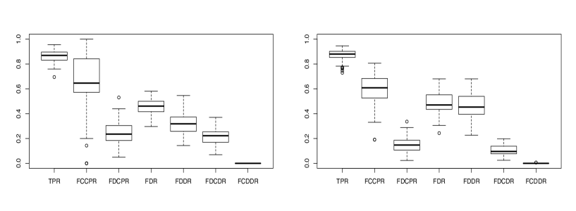
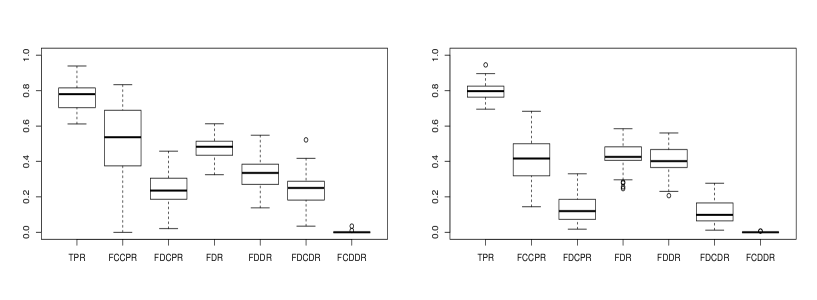
Figure 8: Box-plots of the metrics over 50 i.i.d. DAGs with $d=30$ nodes, sparsities $p=0.1$ (left), and $p=0.2$ (right), regular variation indices $\alpha=2$ (top) and $\alpha=3$ (bottom), and sample size $n=1000$.

For fixed $C,\alpha$ we simulate a sample of $n$ i.i.d. realizations as explained above. These are used to estimate the scalings and extreme dependence measures from Section D.1, which serve as input for Algorithm 2 to identify the MWP pairs. Finally, we estimate the metrics given in Section E.3. The box-plots of Figure 8 are then based on 50 i.i.d. simulation runs, respectively.

When standardizing the observations, as errors for both $\alpha\in\{2,3\}$ we fix $\varepsilon_{1}=0.25,\,\varepsilon_{2}=0.01,\,\varepsilon_{3}=0.07,\,\varepsilon_{4}=0.01,\,\varepsilon_{5}=0.07$. The selected ones are mainly due to simulation experience, taking into account both the pre-asymptotic setting and the influence of the noise. Similar to Klüppelberg and Krali [2021], we set $a=1.0001$.

Finally, regarding the choices of the thresholds, for the sample size $n=1000$ we set $k_{1}=200$ and $k_{2}=100$, while for $n=5000$, $k_{1}=500$ and $k_{2}=200$.

E.3 Evaluation metrics and results

In this section and in Appendix F we present the results of our simulation study using the metrics defined below to evaluate the predictive performance for the $50$ runs.

Our focus is on the MWP from Definition 1.1 for every pair of nodes in a DAG. For the estimator $\hat{\rm MWP}_{k}$ we use Theorem 3.13 in combination with the estimates in Section 4. We also involve true causal pairs (the set CP), true dependent pairs (the set DP), and those in ICP (the pairs in CP but in inverse index order).

We define the following quantities for each DAG $\mathcal{D}_{k}$ with nodes $V_{\mathcal{D}_{k}}$ for $k\in\{1,\dots,50\}$,

• $\hat{\rm MWP}_{k}$– the set of estimated pairs of nodes in MWP for $\mathcal{D}_{k}$;

• ${\rm MWP}_{\mathcal{D}_{k}}$– the set of pairs of nodes in MWP for $\mathcal{D}_{k}$;

• ${\rm MWP}^{c}_{\mathcal{D}_{k}}$– the set of pairs of nodes in MWP^c for $\mathcal{D}_{k}$; here $(X_{i},X_{m})$ are not a RMLM or they could be independent, hence a degenerate RMLM;

• ${\rm CP}_{\mathcal{D}_{k}}=\{(i,m)\in V_{\mathcal{D}_{k}}\times V_{\mathcal{D}_{k}}:m\in{\rm An}(i)\}$ ;

• ${\rm DP}_{\mathcal{D}_{k}}=\{(i,m)\in V_{\mathcal{D}_{k}}\times V_{\mathcal{D}_{k}}:\sigma_{im}^{2}>0\}$;

• ${\rm ICP}_{\mathcal{D}_{k}}=\{(m,i)\in V_{\mathcal{D}_{k}}\times V_{\mathcal{D}_{k}}:(i,m)\in{\rm CP}_{\mathcal{D}_{k}}\}$.

The reported metrics are standard, representing True/False Positive Rates, and False Discovery Rates, see for instance Fawcett [2006] for standard formulas. However, since we measure the metrics across various categories of causal dependence, we extend them via the following formulas:

• True Positive Rate:

  $${\rm TPR}_{k}=\frac{\#\{\hat{{\rm MWP}}_{k}\cap{\rm MWP}_{\mathcal{D}_{k}}\}}{\#\{{\rm MWP}_{\mathcal{D}_{k}}\}};$$

• False Causal and Confounder Positive Rate:

  $${\rm FCCPR}_{k}=\frac{\#\{\hat{{\rm MWP}}_{k}\cap{\rm MWP}^{c}_{\mathcal{D}_{k}}\cap{\rm CP}_{\mathcal{D}_{k}}\}}{\#\{{\rm MWP}^{c}_{\mathcal{D}_{k}}\cap{\rm CP}_{\mathcal{D}_{k}}\}},$$

  which gives the proportion of estimated causal non-MWPs amongst causal non-MWPs, exemplified in $\mathcal{D}_{2}$ in Fig. 1;

• False Dependence Causal Positive Rate:

  $${\rm FDCPR}_{k}=\frac{\#\{\hat{{\rm MWP}}_{k}\cap{\rm DP}_{\mathcal{D}_{k}}\cap{\rm CP}^{c}_{\mathcal{D}_{k}}\}}{\#\{{\rm DP}_{\mathcal{D}_{k}}\cap{\rm CP}^{c}_{\mathcal{D}_{k}}\}},$$

  which gives the proportion of estimated dependent and non-causal MWPs amongst dependent non-causal pairs, exemplified in $\mathcal{D}_{3}$ in Fig. 1;

• False Discovery Rate:

  $${\rm FDR}_{k}=\frac{\#\{\hat{{\rm MWP}}_{k}\cap{\rm MWP}^{c}_{\mathcal{D}_{k}}\}}{\#\{\hat{{\rm MWP}_{k}}\}};$$

• False Dependence Discovery Rate:

  $${\rm FDDR}_{k}=\frac{\#\{\hat{{\rm MWP}}_{k}\cap{\rm MWP}^{c}_{\mathcal{D}_{k}}\cap{\rm DP}_{\mathcal{D}_{k}}\}}{\#\{\hat{{\rm MWP}}_{k}\cap{\rm DP}_{\mathcal{D}_{k}}\}},$$

  which gives the proportion of estimated dependent non-MWPs amongst estimated dependent MWPs;

• False Dependence Causal Discovery Rate:

  $${\rm FDCDR}_{k}=\frac{\#\{\hat{{\rm MWP}}_{k}\cap{\rm DP}_{\mathcal{D}_{k}}\cap{\rm CP}^{c}_{\mathcal{D}_{k}}\}}{\#\{\hat{{\rm MWP}}_{k}\cap{\rm DP}_{\mathcal{D}_{k}}\}},$$

  which gives the proportion of estimated non-causal relations amongst estimated dependent MWPs;

• False Causal Direction Discovery Rate:

  $${\rm FCDDR}_{k}=\frac{\#\{\hat{{\rm MWP}}_{k}\cap{\rm ICP}_{\mathcal{D}_{k}}\}}{\#\{\hat{{\rm MWP}}_{k}\cap{\rm DP}_{\mathcal{D}_{k}}\}},$$

  which gives the proportion of inversely estimated causal relations amongst estimated dependent MWPs.

The metrics provide knowledge for each specific type of causal dependence. One can expect an error from a non-causal non-MWP pair can be considered as more severe relative to the case of a causal non-MWP. Hence it is important to distinguish between the various sources of errors. For instance, the difference between FDDR and FDCDR gives the contribution to the false discovery rate by the causal non-MWP pairs. The False Positive Rates report whether our new methodology is able to differentiate between the different categories of causal dependence.

Finally, we provide some comments on the simulation results as shown below. We observe a similar trend across the True Positive Rate (TPR), and the two False Positive Rates (FCCPR, FDCPR) for different levels of sparsity and regular variation index. The False Discovery Rates (FDR, FDDR, FDCDR) change in a similar fashion likewise. In general TPR lies above $80\%$ and at a similar level across the three dimensions $20,30,40$, despite a mild reduction as the latter increases. The large variation in the false positive rate, FCCPR, when $d=20$ and particularly for $p=0.1$, is due to the very small number of causal non-MWPs. The setting with $d=40$ and $p=0.1$ implies a large number of non-causal dependent pairs, leading to an increase in both FDCPR and FDCDR. Similarly, for $p=0.2$, the number of non-MWP causal pairs can be very large, in some cases more than double the one in MWP, which leads to the increase in FCCPR and FDDR. Overall, however, we see that the methodology is able to distinguish between the different categories, even when a causal relation is present.

The performance of the algorithm is also affected by the regular variation index $\alpha\in\{2,3\}$, which influences the rate of convergence of the respective component maxima to their limiting Fréchet distributions; see for instance Prop. 2.12 in Resnick [1987]. There is a slight decrease in the true positive rate from $\alpha=2$ to $\alpha=3$, and a larger decrease in the false positive rates; see for instance the metrics FCCPR and FDCPR in the box-plots of Appendix F. Amongst the false discovery rates, we notice that they become slightly lower from $\alpha=2$ to $\alpha=3$ in general.

Concerning the level of sparsity $p$, we observe that the metric FDCPR is higher for lower values of $p$, corresponding to a higher number of non-causal pairs with confounders relative to the causal ones. The difference between FDR and FDDR indicates the presence of independent non-MWPs, and we see that this increases for a lower value of $p$, as expected from a higher level of sparsity.

Finally, a larger sample size leads to an improvement in TPR, and generally to a decrease across all false positive rates and false discovery rates.

Appendix F Appendix: Box-plots from the simulation study

In this section we present box-plots from the simulation study based on data with marginals transformed to Fréchet(2) as described after (E.1).

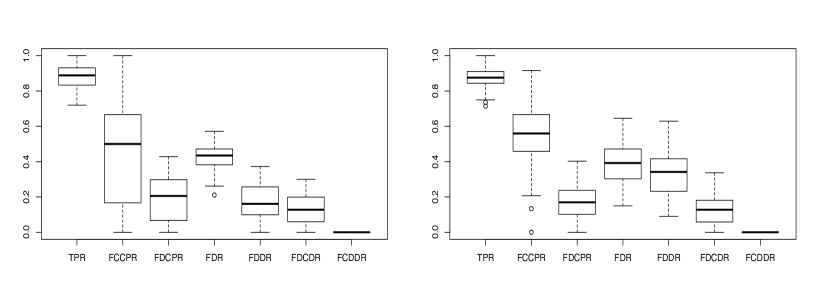
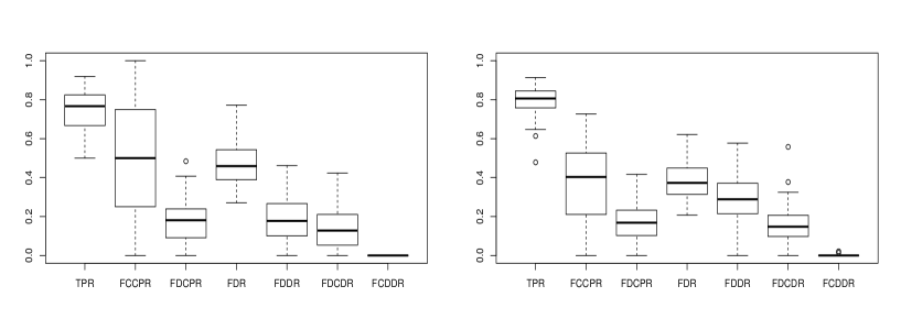
Figure 6: Box-plots of the metrics over 50 i.i.d. DAGs with $d=20$ nodes, sparsities $p=0.1$ (left) and $p=0.2$ (right), regular variation indices $\alpha=2$ (top) and $\alpha=3$ (bottom), and sample size $n=1000$.

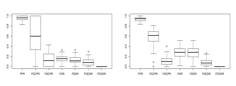
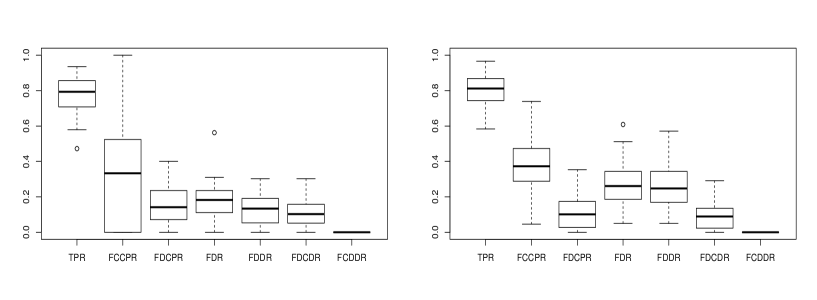
Figure 7: Box-plots of the metrics over 50 i.i.d. DAGs with $d=20$ nodes, sparsities $p=0.1$ (left) and $p=0.2$ (right), regular variation indices $\alpha=2$ (top) and $\alpha=3$ (bottom), and sample size $n=5000$.

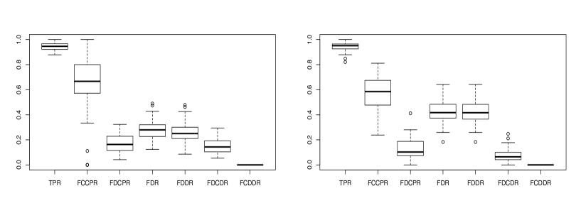
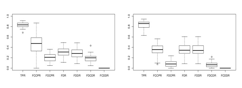
Figure 9: Box-plots of the metrics over 50 i.i.d. DAGs with $d=30$ nodes, sparsities $p=0.1$ (left) and $p=0.2$ (right), regular variation indices $\alpha=2$ (top) and $\alpha=3$ (bottom), and sample size $n=5000$.

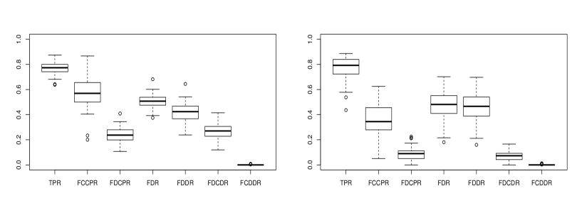
Figure 10: Box-plots of the metrics over 50 i.i.d. DAGs with $d=40$ nodes, sparsities $p=0.1$ (left) and $p=0.2$ (right), regular variation indices $\alpha=2$ (top) and $\alpha=3$ (bottom), and sample size $n=1000$.

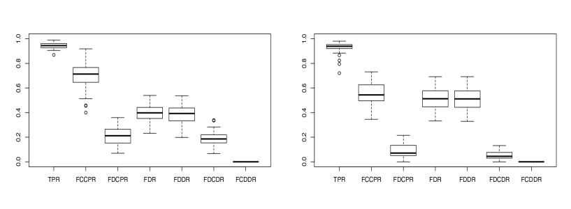
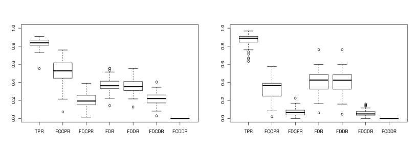
Figure 11: Box-plots of the metrics over 50 i.i.d. DAGs with $d=40$ nodes, sparsities $p=0.1$ (left) and $p=0.2$ (right), regular variation indices $\alpha=2$ (top) and $\alpha=3$ (bottom), and sample size $n=5000$.

References

- Amendola et al. (2022) C. Amendola, C. Klüppelberg, S. Lauritzen, and N. Tran. Conditional independence in max-linear Bayesian networks. The Annals of Applied Probability, 32:1–45, 2022.
- Asenova and Segers (2022) S. Asenova and J. Segers. Max-linear graphical models with heavy-tailed factors on trees of transitive tournaments. arXiv:2209.14938, 2022.
- Basrak et al. (2002) B. Basrak, R. A. Davis, and T. Mikosch. Regular variation of GARCH processes. Stochastic Processes and their Applications, 99(1):95–115, 2002.
- Beirlant et al. (2004) J. Beirlant, Y. Goegebeur, J. Segers, and J. Teugels. Statistics of Extremes: Theory and Applications. Wiley, Chichester, 2004.
- Bickel and Wichura (1971) P. J. Bickel and M. J. Wichura. Convergence criteria for multiparameter stochastic processes and some applications. The Annals of Mathematical Statistics, 42(5):1656–1670, 1971.
- Billingsley (1999) P. Billingsley. Convergence of Probability Measures. John Wiley & Sons, 1999.
- Buck and Klüppelberg (2021) J. Buck and C. Klüppelberg. Recursive max-linear models with propagating noise. Electronic Journal of Statistics, 15(2):4770–4822, Oct 2021. doi: 10.1214/21-EJS1903.
- Butkovič (2010) P. Butkovič. Max-linear Systems: Theory and Algorithms. Springer, London, 2010.
- Chautru (2015) E. Chautru. Dimension reduction in multivariate extreme value analysis. Electronic Journal of Statistics, 9:383–418, 2015.
- Cooley and Thibaud (2019) D. Cooley and E. Thibaud. Decompositions of dependence for high-dimensional extremes. Biometrika, 106(3):587–604, 2019.
- Davis et al. (2013) R.A. Davis, C. Klüppelberg, and C. Steinkohl. Statistical inference for max-stable processes in space and time. Journal of the Royal Statistical Society, Series B, 75(5):791–819, 2013.
- Davison et al. (2019) A. Davison, R. Huser, and E. Thibaud. Spatial extremes. In Handbook of Environmental and Ecological Statistics. CRC Press, 2019. doi: 10.1201/9781315152509-31. Chapter 31.
- de Fondeville and Davison (2022) R. de Fondeville and A. C. Davison. Functional peaks-over-threshold analysis. Journal of the Royal Statistical Society Series B: Statistical Methodology, 84(4):1392–1422, 2022.
- de Haan and Ferreira (2006) L. de Haan and A. Ferreira. Extreme Value Theory: An Introduction. Springer, New York, 2006.
- Embrechts et al. (1997) P. Embrechts, C. Klüppelberg, and T. Mikosch. Modelling Extremal Events for Insurance and Finance. Springer, Heidelberg, 1997.
- Engelke and Hitz (2020) S. Engelke and A. S. Hitz. Graphical models for extremes. Journal of the Royal Statistical Society: Series B, 82(4):871–932, 2020.
- Engelke and Ivanovs (2021) S. Engelke and J. Ivanovs. Sparse structures for multivariate extremes. Annual Review of Statistics and Its Application, 8(1):241–270, 2021. doi: 10.1146/annurev-statistics-040620-041554.
- Engelke and Volgushev (2023) S. Engelke and S. Volgushev. Structure learning for extremal tree models. Journal of the Royal Statistical Society: Series B, 2023. To appear.
- Engelke et al. (2022) S. Engelke, M. Lalancette, and S. Volgushev. Learning extremal graphical structures in high dimensions. arXiv:2111.00840, 2022.
- Fawcett (2006) T. Fawcett. An introduction to roc analysis. Pattern Recognition Letters, 27(8):861–874, 2006.
- Fougerès et al. (2013) A. L. Fougerès, C. Mercadier, and J. P. Nolan. Dense classes of multivariate extreme value distributions. Journal of Multivariate Analysis, 116:109–129, 2013.
- Gissibl and Klüppelberg (2018) N. Gissibl and C. Klüppelberg. Max-linear models on directed acyclic graphs. Bernoulli, 24(4A):2693–2720, 2018.
- Gissibl et al. (2018) N. Gissibl, C. Klüppelberg, and M. Otto. Tail dependence of recursive max-linear models with regularly varying noise variables. Econometrics and Statistics, 6:149 – 167, 2018.
- Gissibl et al. (2021) N. Gissibl, C. Klüppelberg, and S. Lauritzen. Identifiability and estimation of recursive max-linear models. Scandinavian Journal of Statistics, 48(1):188–211, 2021.
- Gnecco et al. (2020) N. Gnecco, N. Meinshausen, J. Peters, and S. Engelke. Causal discovery in heavy-tailed models. Annals of Statistics, 2020. to appear, arXiv:1908.05097.
- Goix et al. (2016) N. Goix, A. Sabourin, and S. Clémençon. Sparse representation of multivariate extremes with applications to anomaly ranking. In Artificial Intelligence and Statistics, pages 75–83. PMLR, 2016.
- Gong et al. (2022) Y. Gong, P. Zhong, T. Opitz, and R. Huser. Partial tail-correlation coefficient applied to extremal-network learning. arXiv:2210.07351, 2022.
- Haug et al. (2015) S. Haug, C. Klüppelberg, and G. Kuhn. Copula structure analysis based on extreme dependence. Statistics and Its Interface, 8(1):93–107, 2015.
- Ivanoff (1980) B. G. Ivanoff. The function space (D, ). Canadian Journal of Statistics, 8(2):179–191, 1980.
- Janßen and Wan (2020) A. Janßen and P. Wan. -means clustering of extremes. Electronic Journal of Statistics, 14(1):1211–1233, 2020.