Abstract

In this paper, we present a toolbox for interval analysis in numpy, with an application to formal verification of neural network controlled systems. Using the notion of natural inclusion functions, we systematically construct interval bounds for a general class of mappings. The toolbox offers efficient computation of natural inclusion functions using compiled C code, as well as a familiar interface in numpy with its canonical features, such as $n$-dimensional arrays, matrix/vector operations, and vectorization. We then use this toolbox in formal verification of dynamical systems with neural network controllers, through the composition of their inclusion functions.

1 Introduction

Interval analysis is a classical field that provides a computationally efficient approach for propagating errors by computing function bounds Jaulin et al. (2001). It has been successfully used for floating point error bounding in numerical and scientific analysis Hickey et al. (2001). Interval bounds are often used for dynamical systems: (i) in reachability analysis, using methods such as Differential Inequalities Scott & Barton (2013) and Mixed Monotonicity Meyer et al. (2019); Abate et al. (2021); (ii) for invariant set computation Abate & Coogan (2020). Recently, interval analysis has been increasingly used for the verification of learning algorithms: (i) standalone neural network verification approaches such as Interval Bound Propogation Gowal et al. (2019); (ii) in-the-loop neural network control system verification approaches including simulation-guided approaches Xiang et al. (2021), POLAR Huang et al. (2022) and ReachMM Jafarpour et al. (2023).

Since all of these techniques use a similar suite of tools, there is value in creating an efficient, user-friendly toolbox for general interval analysis. Python has become the standard for the learning community, and as such there are several existing tools for interval arithmetic. However, they come with key drawbacks: pyinterval does not natively support interval vectors and matrices, and portion supports lists of intervals, but not matrix and vector operations.

Contributions

In this paper, we introduce a novel interval analysis framework called npinterval, implemented in numpy Harris et al. (2020), the computational backbone of most scientific Python packages. This framework is built upon the notion of inclusion functions, which provide interval bounds on the output of a given function. We first define tight inclusion functions for several elementary functions, then use Theorem 2.3 to build natural inclusion functions for a more general class of composed functions. The proposed package extends the prominent benefits of numpy directly to interval analysis, including its efficiency with compiled C implementations, versatility with $n$-dimensional arrays, matrix/vector operations, vectorization, and its familiar user interface. We then demonstrate its utility through an application in formal verification of neural network controlled systems, by composing CROWN Zhang et al. (2018), a state-of-the-art neural network verification method with a natural inclusion functions of the system in Theorem 3.4. The proofs of all the Theorems are presented in Appendix B.

Notation

We denote the standard partial order on $\mathbb{R}^{n}$ by $\leq$, i.e., for $x,y\in\mathbb{R}^{n}$, $x\leq y$ if and only if $x_{i}\leq y_{i}$ for all $i\in\{1,\ldots,n\}$. A (bounded) interval of $\mathbb{R}^{n}$ is a set of form $\{z:\underline{x}\leq z\leq\overline{x}\}=:[\underline{x},\overline{x}]$ for some endpoints $\underline{x},\overline{x}\in\mathbb{R}^{n}$, $\underline{x}\leq\overline{x}$. Let $\mathbb{IR}^{n}$ denote the set of all intervals on $\mathbb{R}^{n}$. We also use the notation $[x]\in\mathbb{IR}^{n}$ to denote an interval when its endpoints are not relevant or implicitly understood to be $\underline{x}$ and $\overline{x}$. For every two vectors $v,w\in\mathbb{R}^{n}$ and every $i\in\{1,\ldots,n\}$, we define the vector $v_{\{i:w\}}\in\mathbb{R}^{n}$ by $\left(v_{\{i:w\}}\right)_{j}=\begin{cases}v_{j}&j\neq i\\ w_{j}&j=i.\end{cases}$. For a function $f:\mathbb{R}^{n}\to\mathbb{R}^{m}$ and a set $\mathcal{X}\subseteq\mathbb{R}^{n}$, define the set-valued extension $f(\mathcal{X})=\{f(x):x\in\mathcal{X}\}$. For two vectors $x,y\in\mathbb{R}^{n}$, let $(x,y)\in\mathbb{R}^{2n}$ denote their concatenation.

2 Interval Analysis

2.1 Interval Arithmetic

Interval analysis extends operations and functions to intervals Jaulin et al. (2001). For example, if we know that some number $a\in[\underline{a},\overline{a}]$, and $b\in[\underline{b},\overline{b}]$, it is easy to see that the sum $(a+b)\in[\underline{a}+\underline{b},\overline{a}+\overline{b}]$.

Definition 2.1 (Inclusion Function Jaulin et al. (2001)).

Given a function $f:\mathbb{R}^{n}\to\mathbb{R}^{m}$, the interval function $[f]:\mathbb{IR}^{n}\to\mathbb{IR}^{m}$ is called an

1. inclusion function for $f$ if, for every $[x]\in\mathbb{IR}^{n}$, $f([x])\subseteq[f]([x])$;

2. $[y]$-localized inclusion function for $f$ if for every $[x]\subseteq[y]$, we have $f([x])\subseteq[f]([x])$.

Moreover, an inclusion function $[f]$ for $f$ is

1. monotone if $[x]\subseteq[y]$ implies that $[f]([x])\subseteq[f]([y])$.

2. tight if, for every $[x]$, $[f]([x])$ is the smallest interval containing $f([x])$.

In the next Theorem, we provide a closed-form expression for the tight inclusion function.

Theorem 2.2 (Uniqueness and Monotonicity of the Tight Inclusion Function).

Given a function $f:\mathbb{R}^{n}\to\mathbb{R}^{m}$, the tight inclusion function can be characterized as

$$[f]([x])=\bigg{[}\inf_{x\in[x]}f(x),\sup_{x\in[x]}f(x)\bigg{]},$$

where the $\inf$ and $\sup$ are taken element-wise, which is unique and monotone.

For some common functions, the tight inclusion function is easily defined. For example, if a function is monotonic, the tight inclusion function is simply the interval created by the function evaluated at its endpoints.

More generally, the tight inclusion function can be alternatively computed using the fact that on a closed and bounded interval, a continuous function will achieve its maximal and minimal values at either the endpoints or a critical value in the interval. For any bounded interval, the tight inclusion function can be evaluated by taking the maximum and minimum of the function on each critical point within and the endpoints of the input interval. Tight inclusion functions for some elementary functions such as $\sin$ and $\cos$ can be defined in this manner (see Table 1). However, when considering general functions, finding the tight inclusion function is often not computationally viable. The following theorem shows a more computational approach, by chaining known inclusion functions.

Theorem 2.3 (Natural Inclusion Functions).

Given a function $f:\mathbb{R}^{n}\to\mathbb{R}^{m}$ defined by a composition of functions with known monotone inclusion functions, i.e., $f=e_{\ell}\circ e_{\ell-1}\circ\cdots\circ e_{1}$, an inclusion function for $f$ is formed by replacing each composite function with its inclusion function, i.e. $[f]=[e_{\ell}]\circ[e_{\ell-1}]\circ\cdots\circ[e_{1}]$ and is called the natural inclusion function. Additionally, if each of the $[e_{j}]$ are monotone inclusion functions, the natural inclusion function is also monotone.

Note that two different decompositions of the function $f$ can lead to two different natural inclusion functions for $f$. Thus, the natural inclusion function is not guaranteed to be the tight inclusion function. For example, consider the function

$$(x+1)^{2}=x^{2}+2x+1,$$

on the interval $[-1,1]$. With the natural inclusion function for the first expression (LHS), the output interval is $([-1,1]+1)^{2}=[0,4]$. With the natural inclusion function for the second expression (RHS), the output interval is $[-1,1]^{2}+2*[-1,1]+1=[0,1]+[-2,2]+1=[-1,4]$. Figure 1 demonstrates this phenomenon in further detail.

2.2 Automated Interval Analysis using npinterval

The main contribution of this paper is to introduce the open source npinterval package, an extension of numpy to allow native support for interval arithmetic. npinterval defines a new interval data-type, internally represented as a tuple of two doubles, $[a]=(a.l,a.u)$. The interval type is fully implemented in C, and therefore the standard operations from Table 1 are all compiled into efficient machine-code executed as needed at runtime. Additionally, since interval is implemented as a dtype in numpy, all of numpy’s prominent features, including $n$-dimensional arrays, fast matrix multiplication, and vectorization, are available to use. In particular, each function from Table 1 is registered as a numpy universal function, allowing for quick, element-wise operation over an $n$-dimensional array. While there are existing interval arithmetic toolboxes, none plug directly into numpy, opting instead to rewrite every operation in Python. While these packages do support the same standard operations from Table 1, they lose the flexibility and utility of numpy, as well as the efficiency of compiled C code.

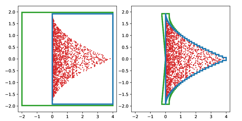
Figure 1: Left: npinterval is used to generate interval approximations for a function $f$ using two different natural inclusion functions. Blue: $f(x_{1},x_{2})=[(x_{1}+x_{2})^{2},4\sin((x_{1}-x_{2})/4)]^{T}$ Green: $f(x_{1},x_{2})=[x_{2}^{2}+2x_{1}x_{2}+x_{2}^{2},4\sin(x_{1}/4)\cos(x_{2}/4)-4\cos(x_{1}/4)\sin(x_{2}/4)]^{T}$. The approximations are generated using the initial set $[-1,1]\times[-1,1]$, and 2000 uniformly sampled ouptuts are shown in red. Right: The same function is analyzed, with the same two natural inclusion functions, but the initial set is partitioned into 1024 uniform sections, and the union of the interval approximations are shown.

3 Interval Reachability of Neural Network Controlled Systems

One application of interval analysis is in reachability analysis of neural network controlled systems. This section revisits and extends the framework considered in Jafarpour et al. (2023).

3.1 Problem Statement

Consider a dynamical system of the following form

$$\dot{x}=f(x,u,w),$$ (1)

where $x\in\mathbb{R}^{n}$ is the system state, $u\in\mathbb{R}^{p}$ is the control input, $w\in\mathcal{W}\subseteq\mathbb{R}^{q}$ is a unknown disturbance input in a compact set $\mathcal{W}$, and $f:\mathbb{R}^{n}\times\mathbb{R}^{p}\times\mathbb{R}^{q}\to\mathbb{R}^{n}$ is a parameterized vector field. We assume that a feedback control policy for the system (1) is given by a $k$-layer fully connected feed-forward neural network $N:\mathbb{R}^{n}\rightarrow\mathbb{R}^{p}$ as follows:

$$\begin{gathered}\xi^{(i)}=\sigma^{(i-1)}\left(W^{(i-1)}\xi^{(i-1)}+b^{(i-1)}\right),\,i=1,\ldots k\\ \xi^{(0)}=x,\quad N(x)=W^{(k)}\xi^{(k)}+b^{(k)}\end{gathered}$$ (4)

where $m_{i}$ is the number of neurons in the $i$-th layer, $W^{(i)}\in\mathbb{R}^{m_{i}\times m_{i-1}}$ is the weight matrix on the $i$-th layer, $b^{(i)}\in\mathbb{R}^{m_{i}}$ is the bias vector on the $i$-th layer, $\xi^{(i)}\in\mathbb{R}^{m_{i}}$ is the $i$-th layer hidden variable and $\sigma_{i}$ is the activation function for the $i$-th layer. Thus, we consider the closed-loop system

$$\dot{x}=f(x,N(x),w)=f^{c}(x,w).$$ (5)

Given an initial time $t_{0}$, an initial state $x_{0}$, and a piecewise continuous mapping $\mathbf{w}:\mathbb{R}\to\mathcal{W}$, denote the trajectory of the system for any $t\geq t_{0}$ as $\phi_{f^{c}}(t,t_{0},x_{0},\mathbf{w})$. Given an initial set $\mathcal{X}_{0}$, we denote the reachable set of $f^{c}$ at some $t\geq t_{0}$:

$$\mathcal{R}_{f}(t,t_{0},\mathcal{X},\mathcal{W})=\left\{\begin{aligned} \phi&{}_{f^{c}}(t,t_{0},x_{0},\mathbf{w}),\,\forall x_{0}\in\mathcal{X}_{0},\\ &w:\mathbb{R}\rightarrow\mathcal{W}\text{ piecewise cont.}\end{aligned}\right\}$$ (6)

One can use the reachable set of the system to verify safety specifications, e.g. by ensuring an empty intersection with unsafe states for all time. However, in general, computing the reachable set exactly is not computationally tractable—instead, approaches typically compute an over-approximation $\overline{\mathcal{R}}_{f^{c}}(t,t_{0},\mathcal{X},\mathcal{W})\supseteq\mathcal{R}_{f^{c}}(t,t_{0},\mathcal{X},\mathcal{W})$. The main challenge addressed in this section is to develop an approach for providing tight over-approximations of reachable sets while remaining computationally tractable for runtime computation.

3.2 Open-loop System Interval Reachability

Previously, Jafarpour et al. (2023) consider a known decomposition function of the open-loop system. The interval analysis framework from Section 2 allows us to extend this theory to remove the need to define a decomposition function a priori.

Assumption 3.1.

For the dynamical system (1), there exists a known monotone inclusion function $[f]$ for $f$.

Using Theorem 2.3, this assumption reduces to knowing a particular form $f=e_{\ell}\circ\cdots\circ e_{1}$ with known monotone inclusion functions for each $e_{j}$, thus removing the need to manually define a decomposition function for $f$.

The open-loop embedding function is defined by:

$$\begin{gathered}\underline{\mathsf{F}}_{i}([x],[u],[w])=\underline{f}_{i}([\underline{x},\overline{x}_{\{i:\underline{x}\}}],[u],[w]),\\ \overline{\mathsf{F}}_{i}([x],[u],[w])=\overline{f}_{i}([\underline{x}_{\{i:\overline{x}\}},\overline{x}],[u],[w]),\end{gathered}$$ (9)

for every $i\in\{1,\ldots,n\}$, where $[f]=[\underline{f},\overline{f}]$ is the monotone inclusion function of $f$, and $\underline{\mathsf{F}},\overline{\mathsf{F}}:\mathbb{IR}^{n}\times\mathbb{IR}^{p}\times\mathbb{IR}^{q}\to\mathbb{R}^{n}$. Using this embedding function, the following embedding dynamics can be defined

$$\begin{bmatrix}\dot{x}\\ \dot{\widehat{x}}\end{bmatrix}=\begin{bmatrix}\underline{\mathsf{F}}([x,\widehat{x}],[u],[w])\\ \overline{\mathsf{F}}([x,\widehat{x}],[u],[w])\end{bmatrix},$$ (10)

where $(x,\widehat{x})\in\mathbb{R}^{2n}$, $x\leq\widehat{x}$.

Theorem 3.2 (Open-Loop System Interval Reachability).

Let $t\mapsto(\underline{x}(t),\overline{x}(t))$ denote the trajectory of the system (10) with initial condition $(\underline{x}_{0},\overline{x}_{0})$, under interval control mapping $[\mathbf{u}]:\mathbb{R}\to\mathbb{IR}^{p}$ and interval disturbance mapping $[\mathbf{w}]:\mathbb{R}\to\mathbb{IR}^{q}$. Let $t\mapsto x(t)$ denote the trajectory of the system (1) with initial condition $x_{0}$, under control $\mathbf{u}:\mathbb{R}\to\mathbb{R}^{p}$ and disturbance $\mathbf{w}:\mathbb{R}\to\mathcal{W}$. If $x_{0}\in[\underline{x}_{0},\overline{x}_{0}]$, $\mathbf{u}(t)\in[\mathbf{u}](t)$, and $\mathbf{w}(t)\in[\mathbf{w}](t)$ for every $t\geq t_{0}$, then

$$x(t)\in[\underline{x}(t),\overline{x}(t)],\quad\mbox{ for every }t\geq t_{0}.$$

3.3 Interconnected Closed-Loop System Interval Reachability

While Theorem 3.2 provides a method of over-approximating the system $\eqref{eq:clsys}$ using global bounds on the control input, it disregards all interactions between the neural network controller and the dynamical system.

Assumption 3.3.

For the neural network (4), there exists a known monotone inclusion function $[N]$ for $N$.

For example, one can use CROWN Zhang et al. (2018) to obtain these bounds. Using CROWN, given an interval $[y]$, we can obtain affine upper and lower bounds of the following form

$$\underline{C}_{[y]}x+\underline{d}_{[y]}\leq N(x)\leq\overline{C}_{[y]}x+\overline{d}_{[y]},$$ (11)

valid for any $x\in[y]$, which can be used to create the following monotone $[y]$-localized inclusion function $[N]_{[y]}=[\underline{N}_{[y]},\overline{N}_{[y]}]$, with

$$\begin{gathered}\underline{N}_{[y]}([x])=\underline{C}_{[y]}^{+}\underline{x}+\underline{C}_{[y]}^{-}\overline{x}+\underline{d}_{[y]},\\ \overline{N}_{[y]}([x])=\overline{C}_{[y]}^{+}\overline{x}+\overline{C}_{[y]}^{-}\underline{x}+\overline{d}_{[y]},\\ \end{gathered}$$ (15)

valid for any $[x]\subseteq[y]$. One can then construct the following “hybrid” closed-loop embedding function by interconnecting the open-loop embedding function with the monotone inclusion function for the neural network as follows

$$\begin{gathered}\underline{\mathsf{F}}^{c}_{i}([x],[w])=\underline{f}_{i}([\underline{x},\overline{x}_{\{i:\underline{x}\}}],[N]_{[x]}([\underline{x},\overline{x}_{\{i:\underline{x}\}}]),[w]),\\ \overline{\mathsf{F}}^{c}_{i}([x],[w])=\overline{f}_{i}([\underline{x}_{\{i:\overline{x}\}},\overline{x}],[N]_{[x]}([\underline{x}_{\{i:\overline{x}\}},\overline{x}]),[w]),\\ \end{gathered}$$ (19)

for every $i\in\{1,\ldots,n\}$, and $\underline{\mathsf{F}}^{c},\overline{\mathsf{F}}^{c}:\mathbb{IR}^{n}\times\mathbb{IR}^{q}\to\mathbb{R}^{n}$. Using this embedding function, the following embedding dynamics can be defined

$$\begin{bmatrix}\dot{x}\\ \dot{\widehat{x}}\end{bmatrix}=\begin{bmatrix}\underline{\mathsf{F}}^{c}([x,\widehat{x}],[w])\\ \overline{\mathsf{F}}^{c}([x,\widehat{x}],[w])\end{bmatrix},$$ (20)

where $(x,\widehat{x})\in\mathbb{R}^{2n}$, $x\leq\widehat{x}$.

Theorem 3.4 (Closed-Loop System Interval Reachability).

Let $t\mapsto(\underline{x}(t),\overline{x}(t))$ denote the trajectory of the system (20) with initial condition $(\underline{x}_{0},\overline{x}_{0})$, under interval disturbance mapping $[\mathbf{w}]:\mathbb{R}\to\mathbb{IR}^{q}$. Let $t\mapsto x(t)$ denote the trajectory of the closed-loop system (5) with initial condition $x_{0}$, under disturbance $\mathbf{w}:\mathbb{R}\to\mathcal{W}$. If $x_{0}\in[\underline{x}_{0},\overline{x}_{0}]$ and $\mathbf{w}(t)\in[\mathbf{w}](t)$ for every $t\geq t_{0}$, then

$$x(t)\in[\underline{x}(t),\overline{x}(t)],\quad\mbox{ for every }t\geq t_{0}.$$

3.4 Experiments

Vehicle Model

Consider the nonlinear dynamics of a vehicle adopted from Polack et al. (2017):

$$\dot{p_{x}} =v\cos(\phi+\beta(u_{2})) \dot{\phi} =\frac{v}{\ell_{r}}\sin(\beta(u_{2}))$$ (21)

$$\dot{p_{y}} =v\sin(\phi+\beta(u_{2})) \dot{v} =u_{1}.$$ (22)

where $[p_{x},p_{y}]^{\top}\in\mathbb{R}^{2}$ is the displacement of the center of mass, $\phi\in[-\pi,\pi)$ is the heading angle in the plane, and $v\in\mathbb{R}_{\geq 0}$ is the speed of the center of mass. Control input $u_{1}$ is the applied force, input $u_{2}$ is the angle of the front wheels, and $\beta(u_{2})=\mathrm{arctan}\left(\frac{\ell_{f}}{\ell_{f}+\ell_{r}}\tan(u_{2})\right)$ is the slip slide angle. Let $x=[p_{x},p_{y},\phi,v]^{\top}$ and $u=[u_{1},u_{2}]^{\top}$. We use the neural network controller ($4\times 100\times 100\times 2$ ReLU) defined in Jafarpour et al. (2023), which is applied at evenly spaced intervals of $0.25$ seconds apart. This neural network is trained to mimic an MPC that stabilizes the vehicle to the origin while avoiding a circular obstacle centered at $(4,4)$ with a radius of $2$.

The natural inclusion function is constructed using npinterval with Table 1, and the monotone inclusion function (15) is computed using autoLiRPA Xu et al. (2020). The closed-loop embedding function (20) is then used to over-approximate the reachable set of the system using Theorem 3.4. The dynamics are simulated using Euler integration with a step size of $0.05$. The results are shown in Figure 2.

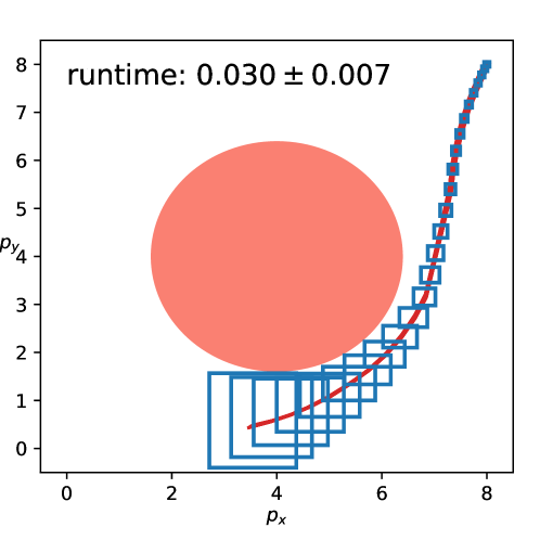
Figure 2: The over-approximated reachable set of the nonlinear vehicle model in the $p_{x}$-$p_{y}$ coordinates are shown in blue for the initial set $[7.95,8.05]^{2}\times[-\frac{2\pi}{3}-0.005,-\frac{2\pi}{3}+0.005]\times[1.995,2.005]$ over the time interval $[0,1.25]$. 100 true trajectories of the system are shown in red, and the average runtime and standard deviation over 100 runs is shown.

4 Conclusion

In this paper, we introduced a framework for interval analysis implemented directly in numpy, called npinterval. The framework provides an automatic way to generate provide interval bounds on the output of a general class of functions. We use this framework to formally verify the output of nonlinear neural network controlled systems. In the future, npinterval will be updated to account for floating point error, as well as to support a wider array of standard inclusion functions.

Appendix A Table of Tight Inclusion Functions and Operations Implemented in npinterval

Table 1: Tight inclusion functions and operations supported by npinterval.

Function/Operation	Tight inclusion function/Implementation
$[a]+c$	$[\underline{a}+c,\overline{a}+c]$
$c*[a]$	$\begin{cases}\left[c\underline{a},c\overline{a}\right]&c\geq 0\\ [c\overline{a},c\underline{a}]&c<0\end{cases}$
$[a]+[b]$	$[\underline{a}+\underline{b},\overline{a}+\overline{b}]$
$[a]-[b]$	$[\underline{a}-\overline{b},\overline{a}-\underline{b}]$
$[a]*[b]$	$[\min\{\underline{a}\underline{b},\underline{a}\overline{b},\overline{a}\underline{b},\overline{a}\overline{b}\},\max\{\underline{a}\underline{b},\underline{a}\overline{b},\overline{a}\underline{b},\overline{a}\overline{b}\}]$
$1/[a]$	$\begin{cases}\left[1/\overline{a},1/\underline{a}\right]&0\notin[a]\\ [-\infty,\infty]&0\in[a]\end{cases}$
$[a]^{n}$	$\begin{cases}[\underline{a}^{n},\overline{a}^{n}]&n\text{ odd}\\ [0,\max\{\underline{a}^{n},\overline{a}^{n}\}]&n\text{ even, }0\in[a]\\ [\min\{\underline{a}^{n},\overline{a}^{n}\},\max\{\underline{a}^{n},\overline{a}^{n}\}]&n\text{ even, }0\notin[a]\end{cases}$
$f([a]),\,f$ mon inc	$[f(\underline{a}),f(\overline{a})]$
$f([a]),\,f$ mon dec	$[f(\overline{a}),f(\underline{a})]$
Trigonometric	See Equations 23 and 24
$\begin{gathered}*[B],\\ \,[A]\in\mathbb{IR}^{n\times p},\,[B]\in\mathbb{IR}^{p\times m}\end{gathered}$	$[\cdot]_{i,j}=\sum_{k=1}^{p}[a_{i,k}]*[b_{k,j}]$

The following is the tight inclusion function for $\sin$,

$$\sin([a])=\begin{cases}[-1,1]&\mathcal{A}_{1}\\ [\underline{s},\overline{s}]&\mathcal{A}_{2}\land((\underline{c},\overline{c})\geq 0)\\ [\overline{s},\underline{s}]&\mathcal{A}_{2}\land((\underline{c},\overline{c})\leq 0)\\ [\min\{\underline{s},\overline{s}\},1]&\mathcal{A}_{2}\land((\underline{c},\overline{c})\geq_{\text{SE}}0)\\ [-1,\max\{\underline{s},\overline{s}\}]&\mathcal{A}_{2}\land((\underline{c},\overline{c})\leq_{\text{SE}}0)\\ [-1,1]&\mathcal{A}_{3}\land((\underline{c},\overline{c})\geq 0)\\ [-1,1]&\mathcal{A}_{3}\land((\underline{c},\overline{c})\leq 0)\\ [\min\{\underline{s},\overline{s}\},1]&\mathcal{A}_{3}\land((\underline{c},\overline{c})\geq_{\text{SE}}0)\\ [-1,\max\{\underline{s},\overline{s}\}]&\mathcal{A}_{3}\land((\underline{c},\overline{c})\leq_{\text{SE}}0)\\ \end{cases},$$ (23)

where $\mathcal{A}_{1}:=(|[a]|>2\pi)$, $\mathcal{A}_{2}:=(\pi<|[a]|\leq 2\pi)$, $\mathcal{A}_{3}=(0<|[a]|\leq\pi)$, $\underline{s}:=\sin(\underline{a})$, $\overline{s}:=\sin(\overline{a})$, and $\underline{c}:=\cos(\underline{a})$, $\overline{c}:=\cos(\overline{a})$. Note that the tight inclusion function for $\cos$ can be defined as $\cos([a])=\sin([a]+\pi/2)$.

$$\tan([a])=\begin{cases}[\tan(\underline{a}),\tan(\overline{a})]&\forall k\in\mathbb{N},\,\frac{\pi}{2}+\pi k\notin[a]\\ [-\infty,\infty]&\exists k\in\mathbb{N},\,\frac{\pi}{2}+\pi k\in[a]\end{cases}$$ (24)

So far, in npinterval, the implemented monotonic functions include $\exp,\log,\arctan,$ and $\operatorname{sqrt}$, and will be extended in the future.

Appendix B Proof of the main results

In this section, we define the southeast order $\leq_{\mathrm{SE}}$ on $\mathbb{R}^{n}$ by $\begin{bmatrix}x\\ y\end{bmatrix}\leq_{\mathrm{SE}}\begin{bmatrix}\widehat{x}\\ \widehat{y}\end{bmatrix}$ if and only if $x\leq\widehat{x}$ and $\widehat{y}\leq y$.

Proof of Theorem 2.2

Take $f:\mathbb{R}^{n}\to\mathbb{R}^{m}$, and fix $[x]\in\mathbb{IR}^{n}$. We need to show that the smallest interval containing $f([x])$ is $\left[\inf_{x\in[x]}f(x),\sup_{x\in[x]}f(x)\right]$.

Fix $i\in\{1,\ldots,n\}$. For contradiction, assume that the smallest interval containing the set $f_{i}([x])$ is not $\left[\inf_{x\in[x]}f_{i}(x),\sup_{x\in[x]}f_{i}(x)\right]$. Then, there are two (non-exclusive) cases:

Case 1: There exists $a>\inf_{x\in[x]}f_{i}(x)$ such that $f_{i}(x)\geq a$ for every $x\in[x]$. However, by the definition of $\inf$, there exists $x^{\prime}\in[x]$ such that $\inf_{x\in[x]}f_{i}(x)<f_{i}(x^{\prime})<a$, which is a contradiction.

Case 2: There exists $b<\sup_{x\in[x]}f_{i}(x)$ such that $f_{i}(x)\leq b$ for every $x\in[x]$. However, by the definition of $\sup$, there exists $x^{\prime}\in[x]$ such that $b<f_{i}(x^{\prime})<\sup_{x\in[x]}f_{i}(x)$, which is a contradiction.

Thus, the smallest interval containing the set $f_{i}([x])$ is $\left[\inf_{x\in[x]}f_{i}(x),\sup_{x\in[x]}f_{i}(x)\right]$. This is true for every $i$, completing the proof.

Proof of Theorem 2.3

We prove the theorem by induction.

Base Case: $m=1$

Since $[e_{1}]$ is an inclusion function for $e_{1}$, we have that $e_{1}\subseteq[e_{1}]([x])$ for any interval $[x]$. Moreover, since $[e_{1}]$ is a monotone inclusion function, we have $[x]\subseteq[y]\implies[e_{1}]([x])\subseteq[e_{1}]([y])$.

Inductive Step: $[e_{m-1}]\circ\cdots\circ[e_{1}]$ monotone inclusion function $\implies$ $[e_{m}]\circ[e_{m-1}]\circ\cdots\circ[e_{1}]$ monotone inclusion function

Assume that $[e_{m-1}]\circ\cdots\circ[e_{1}]$ is a monotone inclusion function for $e_{m-1}\circ\cdots\circ e_{1}$. For every interval $[x]$, we have that $e_{m}\circ e_{m-1}\circ\cdots\circ e_{1}([x])=e_{m}(e_{m-1}\circ\cdots\circ e_{1}([x]))\subseteq e_{m}([e_{m-1}]\circ\cdots\circ[e_{1}]([x]))\subseteq[e_{m}]([e_{m-1}]\circ\cdots\circ[e_{1}]([x]))$, which implies that $[e_{m}]\circ[e_{m-1}]\circ\cdots\circ[e_{1}]$ is an inclusion function for $e_{m}\circ e_{m-1}\circ\cdots\circ e_{1}$.

Moreover, since $[e_{m-1}]\circ\cdots\circ[e_{1}]$ is a monotone inclusion function, we have that for any two intervals $[x]\subseteq[y]$, $[e_{m-1}]\circ\cdots\circ[e_{1}]([x])\subseteq[e_{m-1}]\circ\cdots\circ[e_{1}]([y])$. Since $[e_{m}]$ is monotone, we also have $[e_{m}]([e_{m-1}]\circ\cdots\circ[e_{1}]([x]))\subseteq[e_{m}]([e_{m-1}]\circ\cdots\circ[e_{1}]([y]))$, implying that $[e_{m}]\circ[e_{m-1}]\circ\cdots\circ[e_{1}]$ is a monotone inclusion function.

This completes the proof.

Proof of Theorem 3.2

We define the function $d$ for the open-loop dynamics $f$ (1) as follows:

$$d_{i}(x,\widehat{x},u,\widehat{u},w,\widehat{w}) =\begin{cases}\min_{z\in[x,\widehat{x}],\xi\in[w,\widehat{w}]\atop z_{i}=x_{i},\eta\in[u,\widehat{u}]}f_{i}(z,\eta,\xi),&x\leq\widehat{x},u\leq\widehat{u},w\leq\widehat{w}\\ \max_{z\in[\widehat{x},x],\xi\in[w,\widehat{w}]\atop z_{i}=\widehat{x}_{i},\eta\in[u,\widehat{u}]}f_{i}(z,\eta,\xi),&\widehat{x}\leq x,\widehat{u}\leq u,\widehat{w}\leq w,\end{cases}$$ (25)

and we consider the following dynamical system on $\mathbb{R}^{2n}$:

$$\frac{d}{dt}\begin{bmatrix}x\\ \widehat{x}\end{bmatrix}=\begin{bmatrix}d(x,\widehat{x},u,\widehat{u},w,\widehat{w})\\ d(\widehat{x},x,\widehat{u},u,\widehat{w},w)\end{bmatrix}$$ (26)

The trajectory of the embedding system (26) with the control input $\left[\begin{smallmatrix}u\\ \widehat{u}\end{smallmatrix}\right]=\left[\begin{smallmatrix}\underline{u}\\ \overline{u}\end{smallmatrix}\right]$ and disturbance $\left[\begin{smallmatrix}w\\ \widehat{w}\end{smallmatrix}\right]=\left[\begin{smallmatrix}\underline{w}\\ \overline{w}\end{smallmatrix}\right]$ starting from $\left[\begin{smallmatrix}\underline{x}_{0}\\ \overline{x}_{0}\end{smallmatrix}\right]$ is denoted by $t\mapsto\left[\begin{smallmatrix}\underline{x}^{o}(t)\\ \overline{x}^{o}(t)\end{smallmatrix}\right]$. Note that, by (Abate et al., 2021, Theorem 1), we have $x(t)\in[\underline{x}^{o}(t),\overline{x}^{o}(t)]$, for every $t\in\mathbb{R}_{\geq 0}$. Moreover, for every $i\in\{1,\ldots,n\}$, we get

$$d_{i}(x,\widehat{x},u,\widehat{u},w,\widehat{w}) =\min_{z\in[x,\widehat{x}],\xi\in[w,\widehat{w}]\atop z_{i}=x_{i},\eta\in[u,\widehat{u}]}f_{i}(z,\eta,\xi)\geq\underline{\mathsf{F}}_{i}([x,\widehat{x}],[u],[w]),$$ (27)

where the first equality holds by definition of $d$ and second inequality holds by Theorem (2.2). Similarly, one can show that $d_{i}(\widehat{x},x,\widehat{u},u,\widehat{w},w)\leq\overline{\mathsf{F}}_{i}([x,\widehat{x}],[u],[w])$, for every $i\in\{1,\ldots,n\}$. This implies that $\left[\begin{smallmatrix}\underline{\mathsf{F}}_{i}([x,\widehat{x}],[u],[w])\\ \overline{\mathsf{F}}_{i}([x,\widehat{x}],[u],[w])\end{smallmatrix}\right]\leq_{\mathrm{SE}}\left[\begin{smallmatrix}d(x,\widehat{x},u,\widehat{u},w,\widehat{w})\\ d(\widehat{x},x,\widehat{u},u,\widehat{w},w)\end{smallmatrix}\right]$, for every $x\leq\widehat{x}$ and every $w\leq\widehat{w}$ and every $u\leq\widehat{u}$. Note that, by (Abate et al., 2021, Theorem 1), the vector field $\left[\begin{smallmatrix}d(x,\widehat{x},u,\widehat{u},w,\widehat{w})\\ d(\widehat{x},x,\widehat{u},u,\widehat{w},w)\end{smallmatrix}\right]$ is monotone with respect to the southeast order $\leq_{\mathrm{SE}}$ on $\mathbb{R}^{2n}$. Now, we can use (Michel et al., 2008, Theorem 3.8.1), to deduce that $\left[\begin{smallmatrix}\underline{x}(t)\\ \overline{x}(t)\end{smallmatrix}\right]\leq_{\mathrm{SE}}\left[\begin{smallmatrix}\underline{x}^{o}(t)\\ \overline{x}^{o}(t)\end{smallmatrix}\right]$, for every $t\in\mathbb{R}_{\geq 0}$. This implies that $[\underline{x}^{o}(t),\overline{x}^{o}(t)]\subseteq[\underline{x}(t),\overline{x}(t)]$. On the other hand, by (Abate et al., 2021, Theorem 1 and Theorem 2), we know that $x(t)\in[\underline{x}^{o}(t),\overline{x}^{o}(t)]$, for every $t\in\mathbb{R}_{\geq 0}$. This lead to $x(t)\in[\underline{x}(t),\overline{x}(t)]$, for every $t\in\mathbb{R}_{\geq 0}$.

Proof of Theorem 3.4

We define the function $d^{c}$ for the closed-loop system $f^{c}$ (5) as follows:

$$d_{i}^{c}(x,\widehat{x},w,\widehat{w}) =\begin{cases}\min_{z\in[x,\widehat{x}],\xi\in[w,\widehat{w}]\atop z_{i}=x_{i}}f^{c}_{i}(z,N(z),\xi),&x\leq\widehat{x},w\leq\widehat{w}\\ \max_{z\in[\widehat{x},x],\xi\in[w,\widehat{w}]\atop z_{i}=\widehat{x}_{i}}f^{c}_{i}(z,N(z),\xi),&\widehat{x}\leq x,\widehat{w}\leq w.\end{cases}$$ (28)

and we consider the following dynamical system on $\mathbb{R}^{2n}$:

$$\frac{d}{dt}\begin{bmatrix}x\\ \widehat{x}\end{bmatrix}=\begin{bmatrix}d^{c}(x,\widehat{x},w,\widehat{w})\\ d^{c}(\widehat{x},x,\widehat{w},w)\end{bmatrix}$$ (29)

The trajectory of the embedding system (29) with disturbance $\left[\begin{smallmatrix}w\\ \widehat{w}\end{smallmatrix}\right]=\left[\begin{smallmatrix}\underline{w}\\ \overline{w}\end{smallmatrix}\right]$ starting from $\left[\begin{smallmatrix}\underline{x}_{0}\\ \overline{x}_{0}\end{smallmatrix}\right]$ is denoted by $t\mapsto\left[\begin{smallmatrix}\underline{x}^{c}(t)\\ \overline{x}^{c}(t)\end{smallmatrix}\right]$. Note that, by (Abate et al., 2021, Theorem 1 and Theorem 2), we have $x(t)\in[\underline{x}^{c}(t),\overline{x}^{c}(t)]$, for every $t\in\mathbb{R}_{\geq 0}$.

Let $i\in\{1,\ldots,n\}$ and $y\in[x,\widehat{x}]$ be such that $y_{i}=x_{i}$. Note that $[\underline{N}_{[x,\widehat{x}]},\overline{N}_{[x,\widehat{x}]}]$ is an monotone inclusion function for $N$ on $[x,\widehat{x}]$. Moreover, $y\in[x,\widehat{x}_{[i:x]}]\subseteq[x,\widehat{x}]$ and thus

$$\underline{N}_{[x,\widehat{x}]}(x,\widehat{x}_{[i:x]})\leq N(y)\leq\overline{N}_{[x,\widehat{x}]}(x,\widehat{x}_{[i:x]}).$$ (30)

Therefore, for every $i\in\{1,\ldots,n\}$, we get

$$d_{i}^{c}(x,\widehat{x},w,\widehat{w}) =\min_{z\in[x,\widehat{x}],\xi\in[w,\widehat{w}]\atop z_{i}=x_{i}}f^{c}_{i}(z,N(z),\xi)\geq\min_{z\in[x,\widehat{x}],\xi\in[w,\widehat{w}],z_{i}=x_{i}\atop u\in[\underline{N}_{[x,\widehat{x}]}(x,\widehat{x}_{[i:x]}),\overline{N}_{[x,\widehat{x}]}(x,\widehat{x}_{[i:x]})]}f^{c}_{i}(z,u,\xi)$$

$$\geq\underline{f}^{c}_{i}([x,\widehat{x}],[N]_{[x]}({[x,\widehat{x}_{\{i:x\}}]}),[w])=\underline{\mathsf{F}}^{c}_{i}([x,\widehat{x}],[w]),$$ (31)

where the first equality holds by definition of $d^{c}$, the second inequality holds by equation (30), the third inequality holds by Theorem (2.2), and the fourth inequality holds by definition of $\underline{\mathsf{F}}^{c}$ in equation (2.2). Similarly, one can show that $d_{i}^{c}(\widehat{x},x,\widehat{w},w)\leq\overline{\mathsf{F}}^{c}_{i}([x,\widehat{x}],[w])$, for every $i\in\{1,\ldots,n\}$. This implies that $\left[\begin{smallmatrix}\underline{\mathsf{F}}^{c}_{i}([x,\widehat{x}],[w])\\ \overline{\mathsf{F}}^{c}_{i}([x,\widehat{x}],[w])\end{smallmatrix}\right]\leq_{\mathrm{SE}}\left[\begin{smallmatrix}d^{c}(x,\widehat{x},w,\widehat{w})\\ d^{c}(\widehat{x},x,\widehat{w},w)\end{smallmatrix}\right]$, for every $x\leq\widehat{x}$ and every $w\leq\widehat{w}$. Note that, by (Abate et al., 2021, Theorem 1), the vector field $\left[\begin{smallmatrix}d^{c}(x,\widehat{x},w,\widehat{w})\\ d^{c}(\widehat{x},x,\widehat{w},w)\end{smallmatrix}\right]$ is monotone with respect to the southeast order $\leq_{\mathrm{SE}}$ on $\mathbb{R}^{2n}$. Now, we can use (Michel et al., 2008, Theorem 3.8.1), to deduce that $\left[\begin{smallmatrix}\underline{x}(t)\\ \overline{x}(t)\end{smallmatrix}\right]\leq_{\mathrm{SE}}\left[\begin{smallmatrix}\underline{x}^{c}(t)\\ \overline{x}^{c}(t)\end{smallmatrix}\right]$, for every $t\in\mathbb{R}_{\geq 0}$. This implies that $[\underline{x}^{c}(t),\overline{x}^{c}(t)]\subseteq[\underline{x}(t),\overline{x}(t)]$. On the other hand, by (Abate et al., 2021, Theorem 1 and Theorem 2), we know that $x(t)\in[\underline{x}^{c}(t),\overline{x}^{c}(t)]$, for every $t\in\mathbb{R}_{\geq 0}$. This lead to $x(t)\in[\underline{x}(t),\overline{x}(t)]$, for every $t\in\mathbb{R}_{\geq 0}$.

References

- Abate & Coogan (2020) Abate, M. and Coogan, S. Computing robustly forward invariant sets for mixed-monotone systems. In 2020 59th IEEE Conference on Decision and Control (CDC), pp. 4553–4559, 2020. doi:10.1109/CDC42340.2020.9304461.
- Abate et al. (2021) Abate, M., Dutreix, M., and Coogan, S. Tight decomposition functions for continuous-time mixed-monotone systems with disturbances. IEEE Control Systems Letters, 5(1):139–144, 2021. doi:10.1109/LCSYS.2020.3001085.
- Gowal et al. (2019) Gowal, S., Dvijotham, K., Stanforth, R., Bunel, R., Qin, C., Uesato, J., Arandjelovic, R., Mann, T. A., and Kohli, P. Scalable verified training for provably robust image classification. In IEEE/CVF International Conference on Computer Vision (ICCV), pp. 4841–4850, 2019. doi:10.1109/ICCV.2019.00494.
- Harris et al. (2020) Harris, C. R., Millman, K. J., van der Walt, S. J., Gommers, R., Virtanen, P., Cournapeau, D., Wieser, E., Taylor, J., Berg, S., Smith, N. J., Kern, R., Picus, M., Hoyer, S., van Kerkwijk, M. H., Brett, M., Haldane, A., Fernández del Río, J., Wiebe, M., Peterson, P., Gérard-Marchant, P., Sheppard, K., Reddy, T., Weckesser, W., Abbasi, H., Gohlke, C., and Oliphant, T. E. Array programming with NumPy. Nature, 585:357–362, 2020. doi:10.1038/s41586-020-2649-2.
- Hickey et al. (2001) Hickey, T., Ju, Q., and Van Emden, M. H. Interval arithmetic: From principles to implementation. J. ACM, 48(5):1038–1068, sep 2001. ISSN 0004-5411. doi:10.1145/502102.502106.
- Huang et al. (2022) Huang, C., Fan, J., Chen, X., Li, W., and Zhu, Q. POLAR: A polynomial arithmetic framework for verifying neural-network controlled systems. In Automated Technology for Verification and Analysis: 20th International Symposium, ATVA 2022, Virtual Event, October 25-28, 2022, Proceedings, pp. 414–430. Springer, 2022. doi:10.48550/arXiv.2106.13867.
- Jafarpour et al. (2023) Jafarpour, S., Harapanahalli, A., and Coogan, S. Interval reachability of nonlinear dynamical systems with neural network controllers. In Learning for Dynamics and Control Conference, volume 211, pp. 1–14. PMLR, 2023. doi:10.48550/arXiv.2304.03671.
- Jaulin et al. (2001) Jaulin, L., Kieffer, M., Didrit, O., and Walter, É. Applied Interval Analysis. Springer London, 2001. doi:10.1007/978-1-4471-0249-6.
- Meyer et al. (2019) Meyer, P.-J., Devonport, A., and Arcak, M. TIRA: Toolbox for interval reachability analysis. In Proceedings of the 22nd ACM International Conference on Hybrid Systems: Computation and Control, pp. 224–229, 2019. doi:10.1145/3302504.3311808.
- Michel et al. (2008) Michel, A. N., Hou, L., and Liu, D. Stability of Dynamical Systems: Continuous, Discontinuous, and Discrete Systems. Stability of Dynamical Systems: Continuous, Discontinuous, and Discrete Systems. Birkhäuser Boston, 2008. doi:10.1007/978-0-8176-4649-3. URL https://books.google.com/books?id=s4mq1h0elUkC.
- Polack et al. (2017) Polack, P., Altché, F., d’Andréa Novel, B., and de La Fortelle, A. The kinematic bicycle model: A consistent model for planning feasible trajectories for autonomous vehicles? In 2017 IEEE Intelligent Vehicles Symposium (IV), pp. 812–818, 2017. doi:10.1109/IVS.2017.7995816.
- Scott & Barton (2013) Scott, J. K. and Barton, P. I. Bounds on the reachable sets of nonlinear control systems. Automatica, 49(1):93–100, 2013. ISSN 0005-1098. doi:10.1016/j.automatica.2012.09.020.
- Xiang et al. (2021) Xiang, W., Tran, H.-D., Yang, X., and Johnson, T. T. Reachable set estimation for neural network control systems: A simulation-guided approach. IEEE Transactions on Neural Networks and Learning Systems, 32(5):1821–1830, 2021. doi:10.1109/TNNLS.2020.2991090.
- Xu et al. (2020) Xu, K., Shi, Z., Zhang, H., Wang, Y., Chang, K.-W., Huang, M., Kailkhura, B., Lin, X., and Hsieh, C.-J. Automatic perturbation analysis for scalable certified robustness and beyond. Advances in Neural Information Processing Systems, 33, 2020. doi:10.48550/arXiv.2002.12920.
- Zhang et al. (2018) Zhang, H., Weng, T.-W., Chen, P.-Y., Hsieh, C.-J., and Daniel, L. Efficient neural network robustness certification with general activation functions. In Advances in Neural Information Processing Systems, volume 31, pp. 4944–4953, 2018. doi:10.48550/arXiv.1811.00866.