Space-Time Entropy, Space of Singularities
and Gravity Origin: A Case Study

Abstract

To figure out characteristics and valuable information relevant to the earliest conditions of the Big Bang event, despite their non accessibility to cosmological observation, a new definition of entropy sensitive to the variation of the curvature of an homogeneous, isotropic and expanding space-time, allows to quantify and approach the earliest period and conditions that have revealed the last scattering surface from where originates the cosmic microwave background radiation. This paper introduces a new framework via a space-time of singularities that allows to determine the major role and the extreme conditions of the space-time earliest transformation that undergoes matter recombination after its dismantlement by the Big Bang event and traces back the origin of gravity within each singularity of the expanding space-time.

Keywords: Curvature, Entropy, Singularity, Black holes characteristics, Gravity

PACS: 97.60.Lf , 98.80.Bp , 98.80.-K , 04.30.-w , 45.20.D-

AMS: 28D20 , 83C57

1 Introduction

The analysis of the Planck’s CMB image has revealed that the distribution of mass/energy density of the universe is estimated today to 68,3 $\%$ of dark energy, 26,8 $\%$ of dark matter and 4,9$\%$ of normal matter (European spacial agency ESA /Planck). The actors of the universe transformation are estimated for our knowledge but unknown to satisfactory define. Many phenomena in relation with our universe are still unknown including the nature of the dark energy, the nature of the dark matter, the characteristics of the inflationary period, the universe phase transitions, the asymmetry in the average temperatures on opposite hemisphere of the sky (from CMB), and the earliest condition of the universe expansion.The oldest light propagation in the universe that revealed the universe composition and evolution, known as the cosmic microwave background (CMB), is actually related to a young universe of 380 000 years old. The earliest period and conditions to the Big Bang, that allow to understand matter formation after its dismantlement by the Big Bang event, remain not accessible to cosmological observation since light is trapped during that period and there is no traceable direct evidence for what happens during the 380 000 years. Many attempts to explain some earliest conditions can be found and the list is not limited to ([6],[7],[8],[9],[11],[12],[13],[19],[20],[21]).

To access to the earliest condition of the universe expansion, we introduce within this case study a new entropy that associates a state function to an homogeneous, isotropic and expanding space-time, characterized by the space-time curvature variation function of its expansion. Using a frame of an homogeneous, isotropic and expanding space-time introduced in [2] that has revealed interesting developments about phenomena thought to be impossible to explain in geometrical optics, such as to provide an indistinguishable interpretation of the interference pattern observed in the Young’s double slit experiment on the screen and between the slits and the screen, a new understanding of the cause behind the Van Der Waals torque, and the description of the unknown Casimir attraction/repulsion’s mechanism in nanotechnology relevant to the experimental observation [1].

A model of expanding space-time, whose geometry appears roughly homogeneous and isotropic at large scale meanwhile it remains non homogeneous and anisotropic at small scale, can be approached by the accumulation of an infinite family of open balls, with same size, endowed with a discrete simultaneous expansion in all directions, where the simultaneous expansion of each open ball with same size pledges homogeneity, isotropy and simulates the space-time expansion at large scale, meanwhile the appearance of apollonian gaskets of packed open balls with different sizes in each interstice assures the anisotropy and non homogeneity of the space-time at small scale [2]. An illustration of one layer of accumulated family of balls with same size is given in Fig.2, and illustration of 8 packed layers to cover a volume is given in Fig.2, where the interstices are covered with open balls of different sizes as illustrated in (Fig.6 and Fig.6) to take into account the density of the space-time.

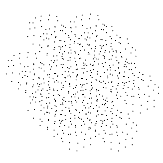
Figure 8: The invisibility of the geometry of the accumulated spheres means that illustration in Fig.8 is the same illustration as in Fig.8 without visualization of the spheres geometry. Matter represented by dots appears to be held in the space with no visible pillars (the spheres) that one can see. Homogeneity and isotropy are approximately verified within this model since there is no privileged direction revealed by observation.

Nevertheless, geometrically speaking the accumulation illustrated in Fig.2 and Fig.2 verifies homogeneity and expansion in all directions, however uniformity is only verified within a limited number of orientations (only six symmetric orientations where the geodesics are the same), so the model is endowed with a relatively anisotropic expansion referred to certain orientations that does not provide the same geodesics in all directions, while the accumulation illustrated in Fig.4 and Fig.4 verifies homogeneity and expansion in all directions, but uniformity of space-time geodesics is only verified within twelve symmetric orientations (debates about homogeneity and isotropy of the universe can be found in [28], [17], [23], [22], [24], [29], [32]). Meanwhile the consideration of matter distribution within the surface of those accumulated open balls approximates homogeneity, isotropy and expansion. An example of illustration of distribution of matter as dots on the surface of a portion of accumulated balls at large scale conveys the idea of homogeneity, isotropy and expansion. Indeed, the increase of the radius of all balls simultaneously within the illustration Fig.8 will increase the distance between dots in all direction and simulates the expansion of the balls boundaries. The observation of matter without geometry in Fig.8 reflects isotropy and homogeneity of matter distribution regardless of the direction of observation, and simulates the expansion of the space where the dots are plotted as the radius of each ball increases simultaneously.

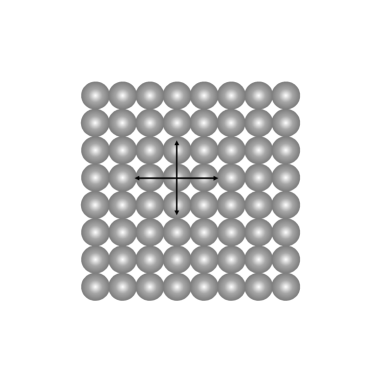
Figure 1: Illustration of one layer of $8\times 8$ packing balls with same size, where each interstice is enclosed between four packing balls. Within this packing model uniformity is only verified within four orientations.

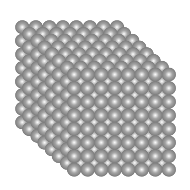
Figure 2: Illustration of a space of packing of 8 layers illustrated in Fig.2 with same size, where each interstice is enclosed between four packing balls. Within this packing model uniformity is only verified within six orientations.

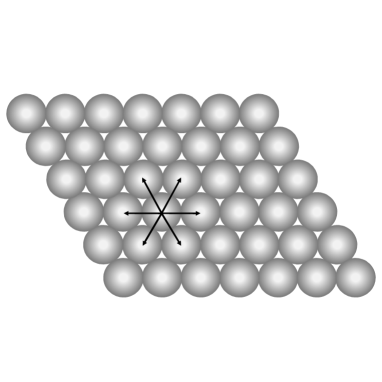
Figure 3: Illustration of one layer of $7\times 6$ packing balls with same size, where each interstice is enclosed between three packing balls. Within this packing model uniformity is only verified within six orientations.

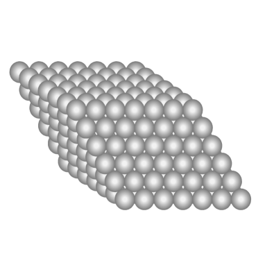
Figure 4: Illustration of a space of packing of 6 layers illustrated in Fig.4 with same size, where each interstice is enclosed between three packing balls. Within this packing model uniformity is only verified within ten orientations. This packing model is more stable than the one illustrated in Fig.2.

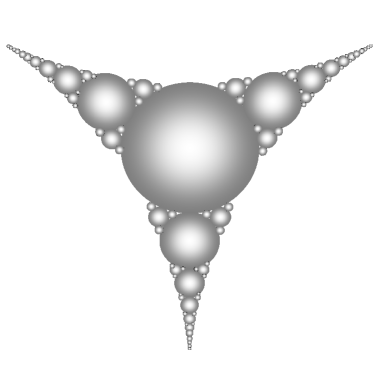
Figure 5: Illustration of packing balls with different sizes to fill the interstice of three packing balls with same size. The biggest ball is located in the center of the interstice. The smaller the number of packing balls with same size that enclose the interstice is, the more stable the packing is. This model is called Apollonian Gasket.

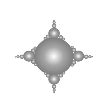
Figure 6: Illustration of packing balls with different sizes to fill the interstice of of four packing balls with same size. The biggest ball is located in the center of the interstice.

To figure out characteristics and valuable information relevant to the earliest conditions of the space-time expansion, the plan of this paper is presented as follow: in section 2 the change of the state function and entropy generation is introduced, as well as its properties. In section 3 we use asymptotic estimation to define singularities and the space-time of singularities. In section 4 an interpretation of the space-time earliest conditions and gravity origin are presented if matter is considered, including a description the initial space before the expansion event, the period of the earliest inflation, the period of the space-time of singularities transformation, gravity origin during the earliest condition of the space-time expansion, the period of primordial space-time when light was released for the first time, and in section 5 the conclusion.

2 Change of the state function and entropy generation

It is known that the change in the state function (entropy) can be determined at thermal equilibrium in terms of the changes of system’s energy and temperature as a heat (Clausius’ entropy [5]), or it can be determined for an isolated system on the total number of micro-states (Boltzmann’s entropy [3], [4]), or it can be determined via a probability distribution of the system (Shannon’s measure of information [30], [31]), or in a generalized quantum gravity entropies such as ([25], [26], [27]). Nevertheless, the different entropy’s definitions mentioned above concern matter characteristics, transformations or distributions, despite the fact that the universe is made of the space-time (the container) and of all form of matter, energy and radiation (the content).

To provide new insight regarding a state function sensitive to the space-time transformation, we use a simple model introduced in [2] of a discrete expanding space-time defined by an infinite accumulation of open balls with same size, where the space-time expansion can be characterized via its local curvature. Nevertheless, some changes in the model and its quantification will be added as follow.

2.1 Quantification adjustment

The transformations of the space-time are quantified in [2] by the sequence ${\mathcal{E}}=({\mathcal{E}_{n}})_{n\geq 0}$ where the initial space-time is ${\mathcal{E}_{0}}$ and the present space-time is ${\mathcal{E}_{n}}$. The integer $n$ represents the subdivision of the time interval of these transformations from the initial space ${\mathcal{E}_{0}}$ to the present space-time ${\mathcal{E}_{n}}$. To include the invisible period for observation that last 380 000 years, minor changes will be considered that concerns the initial condition as well as the used basic element of the modeled space as follow:

1. In this quantification the primordial space-time will be denoted ${\mathcal{E}_{1}}$ rather than ${\mathcal{E}_{0}}$. The primordial space time ${\mathcal{E}_{1}}$ will represent the surface of the last scattering, from where the cosmic microwave background (CMB) comes, around 380 000 years after the Big Bang, when the universe changed from opaque to transparent universe, which makes possible the appearance of the cosmic microwave background when the light was released for the first time.

2. The initial space ${\mathcal{E}_{i}}$ will represent an approximation of the space before the Big Bang, whose basic elements are the limit entities of the basic elements of the primordial space-time ${\mathcal{E}_{1}}$ when their tiny radius tends simultaneously to zero. The earliest transformations will be determined using the characteristics of the limit.

3. We propose to quantify the space-time expansion using a subdivision of the period of time of expansion starting from the primordial space ${\mathcal{E}_{1}}$ to the present space-time ${\mathcal{E}_{n}}$ after $n$ discrete expansions, where $n$ represents the number of subdivisions of the period of time for the discrete transformation of the primordial space-time ${\mathcal{E}_{1}}$ to the space-time ${\mathcal{E}_{n}}$. The bigger the number $n$ of subdivisions of the expansion period is, the smaller the period of time between two successive expansions is, and inversely, the smaller the number $n$ of subdivisions of the expansion period is, the bigger the period of time between two successive expansions is. The space-time will be quantified by the sequence ${\mathcal{E}}=({\mathcal{E}_{n}})_{n\geq 1}$

2.2 Modeling Adjustment

We consider the following model where:

1. The initial space ${\mathcal{E}_{i}}$ is the space whose basic elements are limit entities with a topology close to that of a point, defined by the limit as the radius of the basic elements (the identical spheres) of the primordial space-time ${\mathcal{E}_{1}}$ tends to zero.

2. The primordial space-time ${\mathcal{E}_{1}}$ is the starting space-time at the step 1, defined by an infinite family of packed spheres (rather than open balls) with identical tiny radius $r\in]0,1[$ that cover an Euclidian space (the smallest size that physics can decern from a dimensionless point). These packed identical spheres define the basic elements of the space-time ${\mathcal{E}_{1}}$.

3. The space-time ${\mathcal{E}_{n}}$ is the space-time ${\mathcal{E}_{1}}$ after $n$ simultaneous transformations (expansion) of its basic elements. The space-time ${\mathcal{E}_{n}}$ is represented by an infinity of packed basic elements with identical size, given by spheres with expanding radius quantified by

$$R_{n}={r\Big{(}\prod_{j=1}^{n}a_{j-1}\Big{)}}$$ (1)

where $(a_{n})_{n\geq 0}$ is the sequence of the step-expanding parameters introduced in ([2]), a numerical sequence that quantifies the discrete expansion of the space-time, and satisfies for $a_{0}=1$ the following conditions:

i) for all $n\geq 1$,

$$a_{n}>1,$$ (2)

ii) for all $n\geq 1$,

$$a_{n+1}<a_{n},$$ (3)

iii) the product

$$\prod_{1}^{n}a_{j-1}\qquad\hbox{is convergent,}$$ (4)

and where the intrinsic curvature of each basic element is defined for all $n\geq 1$ by

$$\delta_{n}(r)={1\over R_{n}}={1\over r\Big{(}\prod_{j=1}^{n}a_{j-1}\Big{)}}.$$ (5)

The parameter $a_{j}$ is called the $j^{th}$ quantified expanding parameter of the space-time, and the $\prod_{j=1}^{n}a_{j}$ is called the expanding parameter of the space-time until the step $n$.

4. The interstices: the discrete expansion of the space-time ${\mathcal{E}}=({\mathcal{E}_{n}})_{n>0}$ simulates an homogeneous, isotropic and expanding space-time, whose basic elements are in simultaneous expansion. As the accumulated spheres expand their size, the interstices increase. To simulate a full covered dense space, the interstices are filled with accumulated spheres with different sizes that increase in size together with the basic elements expansion of the space time as illustrated in Fig.6 or in Fig.6. The process to cover the interstices with accumulated spheres of different sizes provides a local fractal character to the model and a local non homogeneity, meanwhile the simultaneous expansion of space-time basic elements provides approximation of homogeneity and isotropy at large scale.

5. The curvature of the expanding space-time ${\mathcal{E}}=({\mathcal{E}_{n}})_{n>0}$ is approximatively determined by the local curvature of the expanding basic elements of the space-time. All basic elements are identical and the local curvature of the space-time is given by the curvature of one basic element, which is a sphere with radius given by (1) for all $n>0$. The curvature of the spheres in the interstice is not considered since it concerns the non-homogeneity (for the small scales).

Thus in the following, the definition of the space-time state function will be related only to the transformation of the basic elements of the space-time that provides homogeneity and isotropy at large scale and generates the space-time expansion.

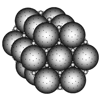
Figure 7: Illustration of a portion of accumulated spheres in which matter is represented by dots on their surface. Since matter exists in a four dimensional space, then the surface of one sphere represents a torsion of an Euclidian space of four dimensions. A 3-sphere cannot be visualized; nevertheless this simple model allows to approximate the visualization of the homogeneity and isotropy.

2.3 Space-time state function

Based on the curvature (5) of the accumulated spheres with same size, we define the space-time state function as follow:

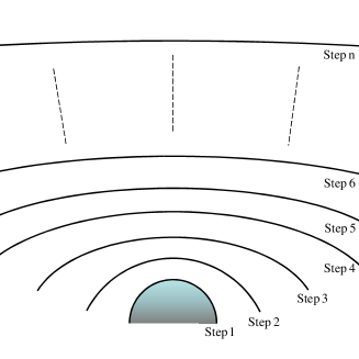
Figure 9: The greater the radius of the basic element is, the lower the curvature of the space-time geodesics is, the more the geodesics approach to the tangent line near the considered points.

Definition 1

Consider the space-time $\mathcal{E}=({\mathcal{E}_{n}})_{n>0}$ where ${\mathcal{E}_{1}}$ is the primordial space-time. For an arbitrary tiny radius $r\in]0,1[$ and an arbitrary finite positive constant k, we define the entropy of space-time $\mathcal{E}$ at the Step n for all $n>0$ as

$$S_{n}(r)=-k\ \ln(\delta_{n}(r)),$$ (6)

where $\delta_{n}(r)={1\over R_{n}}$ is the curvature of the basic elements of radius $R_{n}={r\prod_{1}^{n}a_{j-1}}$ of the space-time ${\mathcal{E}_{n}}$ at the step $n$.

The function (6) is a state function since it is given by an integral that depends only on the lower limit (the curvature of a unit sphere) and the upper limit (the curvature of the basic element of the space-time ${\mathcal{E}_{n}}$ of radius (1)). Indeed, the function (6) can be written as

$$S_{n}(r)=-k\int_{1}^{\delta_{n}(r)}{1\over t}\ dt=-k\ \Big{(}\ln(\delta_{n}(r))-\ln(1)\Big{)}=-k\ \ln(\delta_{n}(r)).$$ (7)

2.4 Quantified entropy generation and entropy generation

Using the above state function given by (6), the quantified change of the state function together with the space-time expansion, denoted by $\Delta S_{n}$, is given by

$$\Delta S_{n}=S_{n+1}(r)-S_{n}(r)$$ (8)

where $S_{n}(r)$ is the state function of the space-time $\mathcal{E}_{n}$ at the Step $n$, and $S_{n+1}(r)$ is the state function of the space-time $\mathcal{E}_{n+1}$ at the Step $n+1$.

Notation

a) ) We call”quantified entropy generation between the steps n and n+1” of the space-time $\mathcal{E}=({\mathcal{E}_{n}})_{n\geq 1}$ and we denote it by $\Delta S_{n}=S_{n+1}-S_{n}$, the quantified change of the state function of successive expansions of the space-time $\mathcal{E}$ for all $n\geq 1$.

b) We call ”Space-time entropy generation between the steps 1 and n” of the space-time $\mathcal{E}=({\mathcal{E}_{n}})_{n\geq 1}$ and we denote it by $\Delta\mathbb{S}_{n}=S_{n}-S_{1}$, the change of the state function between the primordial space-time $\mathcal{E}_{1}$ (at the Step 1) and the present space-time $\mathcal{E}_{n}$ (at the Step $n$ for all $n\geq 1$).

Thus for all $n>0$ the quantified entropy generation between the steps $n$ and $n+1$ of the space-time $\mathcal{E}=({\mathcal{E}_{n}})_{n\geq 1}$ is given by

$$\Delta S_{n}=k\ \ln({\delta_{n}(r)\over\delta_{n+1}(r)})$$ (9)

where $\delta_{n}(r)={1\over R_{n}}$ is the curvature of the basic element of the space-time $\mathcal{E}_{n}$ at the Step $n$, and using (9) we have

$$S_{n+1}(r)=S_{n}(r)+k\ \ln({\delta_{n}(r)\over\delta_{n+1}(r)}).$$ (10)

Remark 1

i) The arbitrary positive constant $k$ in the equality (9) can be considered as the Boltzmann constant if needed. The state function (6) is defined by an increasing function. Indeed, using (5) the local curvature of the space-time ${\mathcal{E}_{n}}$ for all $n\geq 1$ is a decreasing function of $n$ (for an arbitrary constant $r\in]0,1[$), and we have

$$\forall n\geq 1,\qquad\delta_{n+1}(r)<\delta_{n}(r),$$ (11)

which makes (6) an increasing function of $\delta_{n}(r)$ as $n$ increases.

ii) The quantified entropy generation (9) between the steps n and n+1 can be written using integral notation as follow

$$\Delta S_{n}=k\ln\Big{(}{\delta_{n}(r)\over\delta_{n+1}(r)}\Big{)}=-k\ \int_{\delta_{n}(r)}^{\delta_{n+1}(r)}{1\over t}\ dt.$$ (12)

2.5 Properties of the space-time state function

It is known that the curvature measures the local degree of deformation of a curve (or a surface). It is a quantity that measures the speed at which the graph of a given curve (or surface) deviates from the direction of the tangent line in the neighborhood of local points. Since the basic elements of the space-time $\mathcal{E}_{n}$ are expanding spheres, then the equality (8) for all $n\geq 1$ verifies the following:

Property 1

Let $(S_{n})_{n\geq 1}$ be the sequence of state functions of the space-time ${\mathcal{E}}=(\mathcal{E}_{n})_{n\geq 1}$, then the entropy generation between the steps 1 and n of the space-time ${\mathcal{E}}$ verifies for all $n\geq 1$ and $r\in]0,1[$

$$\Delta\mathbb{S}_{n}=S_{n}(r)-S_{1}(r)=k\ln({\delta_{1}(r)\over\delta_{n}(r)}).$$ (13)

Proof: Using the space-time entropy generation (9) between successive steps for all $n\geq 1$, we obtain

$$\begin{array}[]{cc}\Delta S_{n-1}=&S_{n}(r)-S_{n-1}(r)\\ \Delta S_{n-2}=&S_{n-1}(r)-S_{n-2}(r)\\ \vdots\quad\qquad\vdots&\vdots\\ \Delta S_{1}=&S_{2}(r)-S_{1}(r)\end{array}$$ (14)

by adding the $(n-1)$ equalities (14), it gives

$$\Delta S_{n-1}+\Delta S_{n-2}+\ldots+\Delta S_{1}=S_{n}(r)-S_{1}(r)$$ (15)

and using (6), we obtain

$$S_{n}(r)=S_{1}(r)+k\ln({\delta_{1}(r)\over\delta_{n}(r)}),$$ (16)

which allows to conclude.

Property 2

The quantified entropy generation (9) between the steps n and n+1 of the space-time ${\mathcal{E}}=({\mathcal{E}_{n}})_{n\geq 1}$ verifies

$$(i)\ \forall n\geq 1,\quad\Delta S_{n}=0\quad\Longleftrightarrow\quad{\mathcal{E}}=({\mathcal{E}_{n}})_{n>0}\quad\hbox{is a static space-time},$$ (17)

$$(ii)\ \forall n\geq 1,\quad\Delta S_{n}>0\quad\Longleftrightarrow\quad{\mathcal{E}}=({\mathcal{E}_{n}})_{n\geq 1}\quad\hbox{is expanding space-time},$$ (18)

$$(iii)\ \forall n\geq 1,\quad\Delta S_{n}<0\quad\Longleftrightarrow\quad{\mathcal{E}}=({\mathcal{E}_{n}})_{n\geq 1}\quad\hbox{is contracting space-time}.$$ (19)

Proof: (i) For all $n\geq 1$, we have $\Delta S_{n}=0$, then using (9) we have $k\ln\Big{(}{\delta_{n}(r)\over\delta_{n+1}(r)}\Big{)}=0$, which gives

$$k\ln\Big{(}{R_{n+1}\over R_{n}}\Big{)}=0,\quad\forall n\geq 1,$$ (20)

that is to say for all $n\geq 1$, $R_{n+1}=R_{n}$, which characterizes a static space-time for all increasing positive $n$. The converse is evident.

(ii) For all $n\geq 1$, we have $\Delta S_{n}>0$, then using (9), it gives $k\ln({R_{n+1}\over R_{n}})>0$, which gives, for all $n\geq 1$, $\ln(R_{n+1})>\ln(R_{n})$. That is to say, for all $n\geq 1$, $R_{n+1}>R_{n}$, which characterizes an expanding space-time for all increasing positive $n$. The converse is evident.

iii) For all $n\geq 1$, we have $\Delta S_{n}<0$, then we have $-k\ln({R_{n+1}\over R_{n}})>0$, which gives $k\ln({R_{n}\over R_{n+1}})>0$. Then, for all $n\geq 1$, $\ln(R_{n})>\ln(R_{n+1})$. That is to say, for all $n\geq 1$, $R_{n}>R_{n+1}$, which characterizes a contracting space-time for all increasing positive $n$. The converse is evident, which concludes the proof.

Property 3

The quantified entropy generation between the steps n and n+1 of the space-time ${\mathcal{E}}=({\mathcal{E}_{n}})_{n\geq 0}$ measures the space-time quantified expansion, in particular for all $n\geq 1$

$$\Delta S_{n}=k\ln(a_{n})$$ (21)

where $a_{n}$ is the $n^{th}$ space-time expanding parameter from the Step n to the Step n+1.

Proof: The substitution of the curvature (5) in the entropy generation (9) gives

$$\Delta S_{n}=k\ \ln\Big{(}{\delta_{n}(r)\over\delta_{n+1}(r)}\Big{)}=k\ln\Big{(}{R_{n+1}\over R_{n}}\Big{)}=k\ln\Big{(}{r\Big{(}\prod_{i=1}^{n+1}a_{i-1}\Big{)}\over r\Big{(}\prod_{i=1}^{n}a_{i-1}\Big{)}}\Big{)}=k\ln(a_{n}),$$ (22)

which completes the proof.

Proposition 1

i) The quantified entropy generation between the steps n and n+1 of the space-time ${\mathcal{E}}=({\mathcal{E}_{n}})_{n\geq 1}$ for a short period of time between successive steps of expansion verifies

$$\Delta S_{n}\approx 0$$ (23)

ii) The quantified entropy generation between the steps n and n+1 of the space-time ${\mathcal{E}}=({\mathcal{E}_{n}})_{n>0}$ for a large period of time between successive steps of expansion verifies

$$\Delta S_{n}>0$$ (24)

Proof: i) The expanding parameter (4) of the space-time ${\mathcal{E}}=({\mathcal{E}_{n}})_{n>0}$ can be written for $j=i-1$ as

$$\prod_{i=1}^{n}a_{i-1}=\prod_{j=0}^{n-1}a_{j}=e^{\sum_{0}^{n-1}\ln(a_{j})},$$ (25)

and as $n$ tends to the infinity, the sequence (4) converges. Therefore there exists a big $N>0$ such that for all $n\geq N$, $\ln(a_{n})$ tends to 0, which gives for all $n\geq N$, $a_{n}$ tends to 1, then we have for all $n>N$, $a_{n}\approx 1$ that gives using (21)

$$\Delta S_{n}=k\ln(a_{n})\approx 0.$$ (26)

Since $n>N$, then the integer $n$ is big and represents the number of subdivisions of the period of time of the expansion between primordial space-time ${\mathcal{E}_{1}}$ to the space-time ${\mathcal{E}_{n}}$ after $n$ expansions. Therefore the period of time interval between two successive steps of expansion is short, and for this short period of time, the quantified entropy generation (9) verifies (23).

ii) For all $n<N$, the integer $n$ is not big and represents the number of subdivisions of the period of time of the expansion between primordial space-time ${\mathcal{E}_{1}}$ and the space-time ${\mathcal{E}_{n}}$ after $n$ expansions. Therefore, the number of subdivisions of expansion time interval is small, which gives a large period of time between successive steps. Thus for this large period of time, $a_{n}>1$ and since $k$ is a positive number, then we have

$$k\ln(a_{n})>k\ln(1),$$ (27)

and using (21), the inequality gives

$$\Delta S_{n}>0,$$ (28)

which completes the proof.

Proposition 2

If $(S_{n})_{n>0}$ is the sequence of state functions of the space-time ${\mathcal{E}}=({\mathcal{E}}_{n})_{n>0}$, then for all $n>0$,

i) the entropy generation between the steps 1 and n of the space-time ${\mathcal{E}}=({\mathcal{E}}_{n})_{n>0}$ due to the transformation of the primordial space-time ${\mathcal{E}_{1}}$ to the space-time ${\mathcal{E}_{n}}$ is increasing as $n$ increases, and we have

$$\Delta\mathbb{S}_{n}=S_{n}(r)-S_{1}(r)=k\ \ln({\prod_{j=1}^{n}a_{j-1}}),$$ (29)

where $a_{j}$ is the $j^{th}$ quantified expanding parameter of the space-time.

ii) the quantified entropy generation between the steps n and n+1 of the space-time ${\mathcal{E}}=({\mathcal{E}}_{n})_{n>0}$ due to a successive expansion is decreasing as $n$ increases and we have for all $n>0$

$$\Delta S_{n+1}<\Delta S_{n}.$$ (30)

Proof: i) Using the state function (6) and the space local curvature (5), we have for all $n>0$

$$S_{n}(r)=-k\ \ln\Big{(}\delta_{n}(r)\Big{)}=-k\ \ln\Big{(}{1\over r(\prod_{1}^{n}a_{j-1})}\Big{)}=k\ \ln\Big{(}{r(\prod_{1}^{n}a_{j-1})}\Big{)}$$ (31)

then

$$S_{n}(r)=k\ \ln(r)+k\ \ln\Big{(}{\prod_{1}^{n}a_{j-1}}\Big{)}$$ (32)

$$=k\ \ln(r)+k\ \sum_{j=1}^{n}\ln(a_{j-1}),$$

using (6) for $n=1$, it gives $S_{1}(r)=k\ \ln(r)$, then we have

$$S_{n}(r)=S_{1}(r)+k\ \ln({\prod_{j=1}^{n}a_{j-1}})$$ (33)

which gives (29), and since $a_{0}=1$ and $\ln(1)=0$ it gives

$$S_{n}(r)=S_{1}(r)+k\ \sum_{j=2}^{n}\ln(a_{j-1}),$$ (34)

thus for $j=i-1$ the equality (34) becomes

$$S_{n}(r)=S_{1}(r)+k\ \sum_{j=1}^{n-1}\ln(a_{j}),$$ (35)

which gives

$$\Delta\mathbb{S}_{n}=S_{n}(r)-S_{1}(r)=k\sum_{j=1}^{n-1}\ln(a_{j}).$$ (36)

Using (2), we have for all $j>0$, $a_{j}>1$, which gives $\ln(a_{j})>0$, therefore the entropy generation (36) is given by an increasing convergent series with positive terms. Thus the entropy generation (36) of the space-time ${\mathcal{E}}$ is increasing as $n$ increases.

ii) From (21) we have for $j>0$

$$\Delta S_{j}=k\ln(a_{j}),$$ (37)

therefore using (36) the entropy generation $S_{n}(r)-S_{1}(r)$ of the space time ${\mathcal{E}}=({\mathcal{E}_{n}})_{n>0}$ due to the expansion of the space-time from the Step(1) to present time is given by

$$\Delta\mathbb{S}_{n}=S_{n}(r)-S_{1}(r)=\sum_{j=1}^{n-1}\Delta S_{j},$$ (38)

and using the property of the $n^{th}$ quantified expanding parameter (3), we have for all $j>0$

$$\ln(a_{j+1})<\ln(a_{j})$$ (39)

and the use of (37) gives that for all $j>0$

$$\Delta S_{j+1}<\Delta S_{j},$$ (40)

that is to say the quantified entropy generation $\Delta S_{n}$ is decreasing as $n$ increases, which completes the proof.

Remark 2

i) The equality (23) means that the change of space-time curvature remains imperceptible for a considered short period of time between two successive expansions with respect to the total period of time for the expansion of the primordial space-time ${\mathcal{E}_{1}}$ to the present space-time ${\mathcal{E}_{n}}$. However, for the consideration of a large period of time between two successive expansions, the quantified entropy generation(24) is strictly positive.

ii) The quantified entropy generation between the steps n and n+1 of the space-time ${\mathcal{E}}=({\mathcal{E}_{n}})_{n\geq 0}$ is decreasing as $n$ increases (Proposition 2, ii)), meanwhile the space-time entropy between the steps 1 and n of the space-time ${\mathcal{E}}=({\mathcal{E}_{n}})_{n\geq 0}$ is always increasing with a decelerating increase (Proposition 2, i)).

3 Asymptotic estimation, Space of asymptotic basic elements

Within this study, we have used a subdivision of the period of time of the expansion of the space-time ${\mathcal{E}}=({\mathcal{E}_{n}})_{n\geq 0}$ between the primordial space-time ${\mathcal{E}_{1}}$ and the space-time ${\mathcal{E}_{n}}$. However, the transformation from the initial space ${\mathcal{E}_{i}}$ to the primordial space-time ${\mathcal{E}_{1}}$ that models the opaque period of our universe (that last 380 000 years) is not quantified. An intermediary space-time that quantified this period can be found to characterize and evaluate its state function. Indeed, from equality (5) we know that the curvature of the space-time ${\mathcal{E}_{1}}$ is given for a tiny radius $r\in]0,1[$ by

$$\delta(r)={1\over r},$$ (41)

then as the radius $r$ of each basic element of the space-time ${\mathcal{E}_{1}}$ tends to zero, the local curvature $\delta(r)$ of the basic element of the space-time ${\mathcal{E}_{1}}$ verifies

$$\lim_{r\longrightarrow 0}\delta(r)=\lim_{r\longrightarrow 0}{1\over r}=+\infty.$$ (42)

3.1 Set of asymptotic expanding basic spheres

The divergence of curvature $\delta(r)$ to plus infinity as the radius $r$ tends to zero, means that for all $B>0$ a big real number, there exists a small radius $r_{0}>0$, such that for all $r\in]0,r_{0}[$, the curvature $\delta(r)>B$, which leads to introduce a set of asymptotic expanding spheres, denoted by $\mathcal{B}_{h}(c)$, defined by the disjoint union of spheres $\mathbb{S}(c,r)$ with same center $c$, radius $r\in]0,r_{0}[$ and curvature close to plus infinity, given by:

$$\mathcal{B}_{h}(c)=\bigcup_{0<r<r_{0}}\mathbb{S}(c,r).$$ (43)

The set of expanding asymptotic spheres $\mathcal{B}_{h}(c)$ represents all continuous transformations of one basic element $c$, for all $r\in]0,r_{0}[$, of the initial space ${\mathcal{E}_{i}}$. The curvature of each transformed sphere $\mathbb{S}(c,r)$ remains close to plus infinity. The set $\mathcal{B}_{h}(c)$ is an open ball without center, defined by a disjoint union of imbedded spheres of radius $0<r<r_{0}$. Each sphere is the expansion of previous spheres of smaller radius, and all spheres are homotopic due to the continuous transformation by expansion. The upper limit $r_{0}$ of the radius $r$ of $\mathbb{S}(c,r)$ depends on the arbitrary big constant $B$: whenever we change $B$, the upper limit $r_{0}$ changes.

3.2 Asymptotic expanding space-time ${\mathcal{E}_{r}}$

The spheres from the above set (43) with same radius $r$ and center $c$ for all initial basic element $c\in{\mathcal{E}_{i}}$ can be used to define the basic elements of an asymptotic expanding space-time endowed with infinite curvature as follow:

Definition 2

We call asymptotic expanding space-time and we denote ${\mathcal{E}_{r}}$ for $r\in]0,r_{0}[$, the space-time defined by the infinite family of accumulated spheres $\mathbb{S}(c,r)$ of $\mathcal{B}_{h}(c)$, with same radius $r$ for all initial basic element $c\in{\mathcal{E}_{i}}$.

Property 4

The asymptotic expanding space-time ${\mathcal{E}_{r}}$, for all $r\in]0,r_{0}[$, verifies the following properties:

1. The curvature of the asymptotic expanding space-time ${\mathcal{E}_{r}}$, for all $r\in]0,r_{0}[$, is close to plus infinity.

2. The entropy of the asymptotic expanding space-time ${\mathcal{E}_{r}}$, for all $r\in]0,r_{0}[$, is close to minus infinity.

3. The change of the state function due to a continuous expansion of an asymptotic space-time ${\mathcal{E}_{r_{1}}}$ to an asymptotic space-time ${\mathcal{E}_{r_{2}}}$ for all $0<r_{1}<r_{2}<r_{0}$ is an indeterminate form.

4. The entropy generation of the continuous expansion of an asymptotic expanding space-time ${\mathcal{E}_{r}}$, for all $r\in]0,r_{0}[$, to the primordial space-time ${\mathcal{E}_{1}}$ is close to plus infinity.

Proof: 1. The curvature of the asymptotic expanding space-time ${\mathcal{E}_{r}}$ is close to infinity since it is given by the curvature of identical spheres of the open set $\mathcal{B}_{h}(c)$ defined by (43) for all initial basic element $c\in{\mathcal{E}_{i}}$.

2. From the definition of entropy (6), the entropy $S_{h}$ of the asymptotic expanding space-time ${\mathcal{E}_{r}}$ is close to minus infinity since for all $r<r_{0}$, $\delta(r)={1\over r}$ tends to plus infinity, and then

$$S_{h}=\lim_{\delta(r)\longrightarrow+\infty}-k\ln(\delta(r))=-\infty.$$ (44)

3. To evaluate the entropy generation (or the change in the state function) of the expansion of the asymptotic expanding space-time ${\mathcal{E}_{r_{1}}}$ to the asymptotic expanding space-time ${\mathcal{E}_{r_{2}}}$ for all $0<r_{1}<r_{2}<r_{0}$, we use the difference of their state function denoted respectively $S_{h_{1}}$ and $S_{h_{2}}$. Indeed, since $S_{h_{1}}$ and $S_{h_{2}}$ are given by (44) for $r=r_{1}$, respectively $r=r_{2}$, and since for all $r<r_{0}$, $\delta(r)={1\over r}$ tends to plus infinity, and we have

$$S_{h_{2}}-S_{h_{1}}=(-\infty)-(-\infty),$$ (45)

which is an indeterminate form.

4. To evaluate the entropy generation (or the change in the state function) of the expansion of the asymptotic space-time ${\mathcal{E}_{r}}$, for all $r\in]0,r_{0}[$, to the primordial space-time ${\mathcal{E}_{1}}$, we use the difference of their state function $S_{1}(r)-S_{h}$. Indeed, since $S_{1}(r)$ is positive and finite, and $S_{h}$ is given by (44) then we have

$$S_{1}(r)-S_{h}=S_{1}(r)-(-\infty)=+\infty,$$ (46)

which means that the entropy generation after continuous expansion of the asymptotic expanding space-time ${\mathcal{E}_{r}}$, for $r\in]0,r_{0}[$, to the primordial space-time ${\mathcal{E}_{1}}$ is close to $+\infty$, which completes the proof.

Remark 3

i) In Property 4, 3., despite the fact that the state function of the asymptotic expanding space-time ${\mathcal{E}_{r}}$ approaches minus infinity for any continuous transformation (expansion) of spheres of radius $r\in]0,r_{0}[$, the entropy generation is found to be an indeterminate form, because each one of the entropies $S_{h_{2}}$ and $S_{h_{1}}$ approaches minus infinity, without being equal to minus infinity, that is why the changes of the state function between two distinct asymptotic expanding spaces-time ${\mathcal{E}_{r}}$ is not zero, but unknown.

ii) The characteristics introduced in Property 4 convey divergence before the appearance of the primordial space-time ${\mathcal{E}_{1}}$, which leads to define a singularity, and a space of singularities.

iii) For all $r\in]0,r_{0}[$, the surface area to the volume ratio ${A\over V}=3\delta(r)$ of each basic element of the asymptotic expanding space-time ${\mathcal{E}_{r}}$ is close to plus infinity.

3.3 Singularity, space of singularities

Defining singularity when the geometry becomes unreachable is related to the used theory and formalism of application. Indeed, singularities are seen as an end of the space-time, a pathological set of points where our tools are not defined in mathematics (singularity of a function refers to a point where the function is not defined). In physics, singularities appear unavoidable and carry a potential of great interest. In cosmology, a singularity refers to collapse of matter in which the laws of physics become indistinguishable. A gravitational singularity is a space location where the gravitational field becomes infinite. In this framework singularities carry a potential of great interest and are defined as follow:

Definition 3

We call singularity each sphere of $\mathcal{B}_{h}(c)$, for all basic element $c$ of the initial space-time ${\mathcal{E}_{i}}$, with curvature close to plus infinity and a state function defined by

$$S_{r}(\delta(r))=-k\ \ln(\delta(r)),$$ (47)

that goes to minus infinity as $r$ tends to zero, with $k$ an arbitrary positif constant.

Remark 4

i) A sphere with curvature $\delta(r)={1\over r}$ close to plus infinity, means that for all $B>0$ there exists $r_{0}>0$ such that for all $r\in]0,r_{0}[$, the sphere curvature $\delta(r)={1\over r}$ is close to plus infinity.

ii) The open set $\mathcal{B}_{h}(c)$ given by (43) represents an archive of the continuous transformation of one singularity (all imbedded sphere are homotopic). Indeed $\mathcal{B}_{h}(c)$ is an open ball without center $c$ defined by a disjoint union of imbedded spheres of radius $0<r<r_{0}$, where each sphere is a singularity.

Definition 4

We call space of singularities the space defined by an infinite accumulation of identical singularities.

Remark 5

i) Since the basic elements of the asymptotic expanding space-time ${\mathcal{E}_{r}}$, for all radius $0<r<r_{0}$, are subset of $\mathcal{B}_{h}$ with curvature close to plus infinity, and a state function (47) close to minus infinity, then the asymptotic expanding space-time ${\mathcal{E}_{r}}$ is a space of singularities for all radius $0<r<r_{0}$.

ii) Based on (§2.2., 1.) each basic element of the initial space ${\mathcal{E}_{i}}$ is a limit entity as the radius of each basic element of the primordial space-time ${\mathcal{E}_{1}}$ tends to zero which gives to that limit entity a topology close to that of a point, and indicates that the basic elements of the initial space ${\mathcal{E}_{i}}$ are extremely contracted, with a local entropy $S_{i}$ given by the limit

$$S_{i}=\lim_{r\rightarrow 0}-k\ \ln(\delta(r))=-\infty,$$ (48)

4 Interpretation of the space earliest conditions and gravity origin

Based on this study, the space of singularities is the asymptotic expanding space-time ${\mathcal{E}_{r}}$, for all $0<r<r_{0}\ll 1$, that models the space-time for the period between the Big Bang and the primordial space-time observed after 380 000 years. The consideration of matter, energy and radiation within this model allows to deduce a possible scenario for the origin of gravity, to describe the earliest conditions after the Big Bang and to determine the major role of the space of singularities for the first transformations that led to matter recombination as known today. Indeed, the model quantifies the beginning of the space-time expansion as follow:

4.1 Period of the initial space ${\mathcal{E}_{i}}$

The period of the initial space ${\mathcal{E}_{i}}$ is the period of the space before the Big Bang (§2.2., 1.), when matter, energy and radiation are assumed to be assembled. In this model the initial space before the Big Bang is found to be endowed with local entropy close to minus infinity (48), that corresponds to a space with basic elements extremely contracted with a topology close to that of a point.

4.2 Period of the space of singularities ${\mathcal{E}_{r}}$ and gravity origin

The period of the space of singularities is the closest period after the beginning of the space expansion (the Big Bang), characterized by a space-time of singularities ${\mathcal{E}_{r}}$ for all $r\in]0,r_{0}[$ where the local curvature is infinite (Property 4, Remark 5). The consideration of matter and energy within this model leads to understand the major role of those earliest singularities in the recombination of matter and all forms of energy after being dismantled by the simultaneous expansion of the basic elements of the initial space ${\mathcal{E}_{i}}$ (the Big Bang event).

To evaluate the nearest period of time to the Big Bang event, we assume that the minimal time (the time $t_{0}$) for the expansion of the initial space ${\mathcal{E}_{i}}$ starts when the dismantlement of matter has undergone via the simultaneous expansion of the basic elements of the initial space ${\mathcal{E}_{i}}$, therefore the period of the space of singularities includes the following.

4.2.1 Short period of inflation

The recession of matter in our universe from each other in all directions indicates that matters and all form of energy in the past were assembled within a volume of an extremely contracted initial space ${\mathcal{E}_{i}}$. Any volume in the initial space ${\mathcal{E}_{i}}$ is described by infinite accumulation of extremely contracted limit entities with a topology close to that of a point, and when each limit entity expands to tiny sphere of positive radius, the inflation occurs at the first phase of the space expansion, and each finite volume in the initial space ${\mathcal{E}_{i}}$ expands via expansion of its basic elements and becomes suddenly an infinite space of accumulated spheres of positive radius. Indeed the transformation of each basic element of the initial space ${\mathcal{E}_{i}}$ from extremely contracted limit entities with the topology close to that of a point to a tiny sphere of positive radius induces the following:

1. an instantaneous dismantlement of matter and energy.

2. an instantaneous short period of inflation in the recession motion of parts of the dismantled matter and energy in all direction from each other.

3. the dismantled matter undertakes a local motion in space because of its instantaneous dismantlement (endowed with non null momentum). This local motion is different from the recession motion of matter together with the space expansion.

4. the initial space ${\mathcal{E}_{i}}$ is transformed into the space-time of singularities $({\mathcal{E}_{r})}_{r>0}$ for all $0<r<r_{0}$, where each basic element is characterized by a curvature close to plus infinity and an entropy close to minus infinity.

5. The presence of dismantled matter in motion (with non-null local momentum) within each singularity induces a centripetal acceleration directed toward the center of each singularity given by $\gamma_{r}=v^{2}{\delta_{r}}$, where $v$ is the module of the local speed induced by matter dismantlement and ${\delta_{r}}$ is the singularity’s curvature. This acceleration is responsible for changes in the direction of the velocity of the dismantled matter following the local curvature of the space. Since ${\delta_{r}}$ is close to plus infinity, therefore the dismantled matter experiences a radial acceleration close to plus infinity directed toward the center of each singularity. As the effect of gravity and acceleration are indistinguishable (principle of equivalence), matter experiences a local centripetal gravitational field close to plus infinity.

6. Based on Newton’s second law, a force must cause this centripetal acceleration of magnitude $F=mv^{2}\delta_{r}$. This force bends the motion of the dismantled matter to the space local curvature. It makes the curved motion possible in each singularity. Without this force the motion of the dismantled matter would continue in straight line instead of following the local curvature of the space. It is a kind of frictional force on matter exerted by the local curvature of the space that makes the curved motion possible in an expanding space-time (it is a force that imposes curved motion adapted to the space local curvature).

7. The existence of a centripetal force close to plus infinity within each singularity traps matter just after the beginning of its dismantlement, which makes it uniformly distributed in the space.

Moreover, the existence of a centripetal force close to plus infinity within each singularity makes the trapped dismantled matter experiences an infinite local centripetal compression within each singularity propitious to matter recombination, in particular protons, electrons, neutrons and later on the atomic nucleus.

4.2.2 Gravity origin

The simultaneous expansion of the dimensionless basic elements into basic elements with dimension transforms the initial space ${\mathcal{E}_{i}}$ (where matter and energy were assembled) into the space-time of singularities $({\mathcal{E}_{r})}_{r>0}$ for all $0<r<r_{0}$ at the Big Bang (§4.2.1, item 4.,) and induces:

• a local motion of each part of the dismantled matter, due to its instantaneous transformation from assembled structures to dismantled structures,

• an acceleration of recession motion of the dismantled matter from each other in all direction due to the space expansion,

• a local trap for each part of the dismantled matter within each singularity due to its local motion within a curved space-time.

After the total dismantlement of matter during the instantaneous inflation period, gravity find its origin revealed according to the principle of equivalence between gravity and acceleration. Indeed, based on §4.2.1 items 5. and 6., a centripetal acceleration close to plus infinity appears within each singularity because of the motion of each part of the dismantled matter in an extremely curved space of singularities $({\mathcal{E}_{r})}_{r>0}$ for all $0<r<r_{0}$. According to the Newton’s second law a force must cause this centripetal acceleration, a centripetal force in each singularity of magnitude $F=mv^{2}\delta_{r}$ that accelerates each part of the dismantled matter by changing its velocity direction without changing the speed to makes the curved motion possible. Therefore each part of the dismantled matter in motion experiences a radial gravitational pull (inward the geometrical center of each singularity) responsible for the deviation of its motion from linear to curved.

The appearance of the centripetal gravitational force in each singularity makes the curved motion possible together with the space transformation, and without this local centripetal force the local motion of each part of the dismantled matter would be impossible. The centripetal gravitational force is a kind of frictional force on matter from the expanding space-time that imposes a bend motion of the dismantled matter. However, without the motion of parts of the dismantled matter in the expanding space-time the radial gravitational pull would not exist, which leads to assert the following: gravity exists because matter is never at rest in a curved space-time.

4.2.3 Transformation of the space-time of singularities ${\mathcal{E}_{r}}$

Based on this model the period of the space-time of singularities $({\mathcal{E}_{r})}_{r>0}$ for all $0<r<r_{0}$ corresponds to the period estimated to 380 000 years after the Big Bang, where the gravitational force close to plus infinity within each singularity traps everything including light (since each singularity has the characteristics of a black hole). As the space-time of singularities ${\mathcal{E}_{r}}$ continues to expand via simultaneous expansion of its basic elements by increasing each radius $r$ to $r_{0}$, the local curvature $\delta_{r}={1\over r}$ of the space-time of singularities ${\mathcal{E}_{r}}$ decreases gradually, which reduces the intensity of the centripetal gravitational force within each singularity.

The period where the gravitational field is close to plus infinity within each singularity allows the recombination of the dismantled matter under a decreasing compression close to plus infinity, in particular the recombination of protons, electrons, neutrons, and later atomic nucleus. The gravitational force inside each singularity continues to decrease gradually together with the space-time expansion until it reaches the intensity that allows nucleus to trap electrons and later to form atoms.

Nevertheless, the trapped parts of the dismantled matter experiences a decreasing centripetal gravitational force gradually during this continuous transformation (space-time expansion), until it reaches a critical value (for $r\geq r_{0}$) that allows light to escape for the first time from each singularity, which makes the universe transparent and reveals the surface of the last scattering from where the cosmic microwave background comes. Indeed, as the space-time expands, the primordial singularities of the space-time ${\mathcal{E}_{r}}$ lose simultaneously the characteristics of black hole gradually by the decrease of the local curvature from plus infinity to a certain critical value for $r\geq r_{0}$ that allows the cosmic microwave background to appear for the first time, and then the period of the space of singularities ceases to exist.

However, new singularities with different sizes appear in the interstices of the accumulated primordial basic elements to conserve the density of the space-time. Singularities with different sizes appear and disappear in the interstices functions of their local curvature that decreases gradually from plus infinity together with the space-time expansion, and these new singularities experience a transformation similar to the transformation of the primordial singularities.

4.3 The period of primordial space-time ${\mathcal{E}_{1}}$

Based on this model the period of primordial space-time ${\mathcal{E}_{1}}$ appears when the period the space of singularities ceases to exist and when light is released for the first time approximatively 380 000 years after the Big Bang. Indeed, when gravity reaches an intensity that releases light, matter and energy appear to be distributed all around the previous singularities’ location within an infinite space-time to form the primordial observed space-time ${\mathcal{E}_{1}}$ at the Step 1 of this model that corresponds to the first cosmic microwave background registered after the Big Bang.

This model was simplified to approach the earliest condition for the Big Bang that allowed the recombination of matter and energy after their dismantlement, and leads to understand the uniform distribution of matter and all form of energy.

Nevertheless, since matter exits in a 4 dimensional space-time, therefore the surface of each basic element of the modeled primordial space-time ${\mathcal{E}_{1}}$ must be a distortion of a 4 dimensional Euclidian space, a 3-sphere, and the primordial space-time ${\mathcal{E}_{1}}$ must be an infinite accumulation of 3-spheres, where matter within the expanding space-time ${\mathcal{E}}=({\mathcal{E}_{n}})_{n>0}$ experiences a gravitational force proportional to the space-time curvature of magnitude given by Newton’s second law $F=mv^{2}\delta_{n}(r)$, to the extend that:

• the gravitational field within each basic element of the space-time ${\mathcal{E}}=({\mathcal{E}_{n}})_{n>0}$ experiences a very slow decrease with the space-time expansion. Indeed, based on Proposition 1 the gravitational field within each basic element remains invariant for a short period of time between successive expansions and decreases for a large period of time between successive expansions.

• the interstices of the accumulated basic elements of the space-time ${\mathcal{E}}=({\mathcal{E}_{n}})_{n>0}$ are the locations in which new singularities with different sizes appear when the local curvature remains close to plus infinity, and disappear gradually as the local curvature decreases with the space-time expansion. Each singularity, endowed with characteristics of black holes, traps everything in motion, however without motion the centripetal gravitational ceases to exist despite a curvature close to plus infinity and an entropy close to minus infinity. Each singularity lasts for a period approximatively greater than 380 000 years before to reveal the incubated matter and energy since its gradual transformation depends on the rate of expansion of the primordial basic elements of the space-time ${\mathcal{E}}=({\mathcal{E}_{n}})_{n>0}$.

This scenario is obtained thanks to this case study, that allows to interpret evolution and transformation of matter and energy within an homogeneous and isotopic expanding space-time that expands via simultaneous expansion of its basic elements, and to predict the earliest conditions of the space-time transformation that incubates matter recombination after the total dismantlement by the Big Bang.

5 Conclusion

Using a new definition of entropy sensitive to the evolution of the space-time curvature, within a case study compatible with the fundamental principle of cosmology, new insights are figured out that unravel our comprehension of the earliest condition after the Big Bang. Indeed, this case study allows to access to the earliest conditions of the universe expansion that lasts for a period estimated to 380 000 years after the Big Bang, which is the most chased period in the standard model of cosmology, to the extend that the universe is not accessible for cosmological observation due to the extreme earlier conditions that prevented light from traveling across the universe.

Despite the simplicity of this case study, it leads to define an asymptotic expanding space-time of singularities $(\mathcal{E}_{r})$, $r\in]0,r_{0}[$, endowed locally with extreme characteristics (curvature close to plus infinity, entropy close to minus infinity), and to trace back the expansion of an earliest highly compressed initial space $\mathcal{E}_{i}$, via simultaneous expansion of its limit entities that define the space (its basic elements), and thus to describe the closest period to the beginning of the space-time expansion. The new entropy is defined via a state function that measures the local transformation of the curvature of the space-time from a highly compressed space with infinite curvature to lower compressed space with decreasing curvature.

The consideration of matter and energy within this model provides a surprising interpretation of the earliest phase closest to the beginning of the space expansion that incubates matter recombination after its earliest dismantlement by the Big Bang. The expanding space of singularities traps, distributes and compresses everything locally with a centripetal gravitational force close to plus infinity. The asymptotic space of singularities $(\mathcal{E}_{r})$, $r\in]0,r_{0}[$, quantifies the earliest period of space-time expansion before the period at which the light was released to travel in the universe for the first time. The motion of parts of dismantled matter just after the Big Bang within an extremely curved space-time of singularities $(\mathcal{E}_{r})$ gives birth to an infinite centripetal gravitational attraction directed toward the center of each singularity of the space-time of singularities $(\mathcal{E}_{r})$ and suggests that singularities play the role of incubator for matter and energy recombination after its dismantlement.

Within this model, the space of singularities $(\mathcal{E}_{r})$, $r\in]0,r_{0}[$, characterizes the hidden earliest period of the space-time expansion that lasts approximately 380 000 years, in which subatomic particles as well as atoms were recombined as we know them today after their earliest dismantlement by the Big Bang event. The gradual decrease of the infinite centripetal gravitational attraction within each singularity plays a crucial role in the process of formation of subatomic particles and later atoms when gravity decreases enough to allow nucleus to trap electrons. Indeed, the more the basic elements of the space of singularities expand, the less the local curvature is, and the weaker the intensity of gravitational fields within each singularity is. When the curvature of each singularity is reduced enough together with the space expansion, the centripetal gravitational force decreases and reaches the intensity that allows light to escape and reveals the surface of the last scattering from where the cosmic microwave background comes and is represented by the primordial space-time $\mathcal{E}_{1}$ within this model. Hence this framework allows to:

• study the change of the space-time entropy generation not as a change of a state function based on heat (Clausius’s entropy) or based on the number of micro-states (Boltzmann’s entropy), or based on the measure of information (Shannon’s entropy), but as a change of state function based on curvature transformation of an homogeneous, isotropic and expanding space-time that expands simultaneously via discrete expansion of its basic elements.

• justify the existence of an instantaneous inflation period that occurs when a finite volume defined by an accumulation of an infinity of limit entities with a topology close to that of a point, becomes an infinite space defined by an infinite accumulation of tiny spheres (via simultaneous transformation of each limit entity with a topology close to that of a point into a tiny sphere). This inflation is the first transformation of an initial extremely contracted space $\mathcal{E}_{i}$ to the expanding space of singularities $(\mathcal{E}_{r})$ for $r>0$.

• describe and quantify the earliest phase closest to the beginning of the space expansion (the Big Bang).

• define the space of singularities as the earliest condition for the recombination of matter and energy after their dismantlement by the Big Bang event.

• assert that gravity exists because matter is never at rest in a curved expanding space-time.

References

- [1] Ben Adda F., Fluctuating paths of least time, Schrödinger equation, van der Waals torque and Casimir effect mechanism, International Journal of Geometric Methods in Modern Physics, Vol. 18, No. 11,2150182, (2021).
- [2] Ben Adda F. Porchon H., Infinity of geodesics in a homogeneous and isotropic expanding space-time, International Journal of Geometric Methods in Modern Physics, Vol. 13, No. 4, 1650048, (2016).
- [3] Boltzmann L., Weitere Studien über das Wärmegleichgewicht unter Gas moleku̇len [Further Studies on Thermal Equi-librium Between Gas Molecules], Wien, Ber. 66, 275, (1872).
- [4] Boltzmann L., Über die Beziehung eines allgemeine mechanischen Satzes zum zweiten Haupsatze der Warmetheorie, Sitzungsberichte, K. Akademie der Wissenschaften in Wien, Math.-Naturwissenschaften 75, 67-73, (1877).
- [5] Clausius R., Über verschiedene für die Anwendung bequeme Formen der Hauptgleichungen der mechanischen Wärmetheorie, Annalen der Physik, 125 (7): 353-400, (1865).
- [6] Cai Y. F., Saridakis E. N., Inflation in Entropic Cosmology: Primordial Perturbations and non-Gaussianities, Phys. Lett. B 697, 280-287, (2011).
- [7] Cai R. G., and al., Reheating phase diagram for single-field slow-roll inflationary models, Phys. Rev. D 92, 063506, (2015).
- [8] Cook J. L., and al., Reheating predictions in single field inflation, JCAP 04 , 047, (2015).
- [9] Dai L., and al., Reheating constraints to inflationary models, Phys. Rev. Lett. 113, 041302, (2014).
- [10] Egan, C. A., Lineweaver, C. H., A Larger Estimate of the Entropy of the Universe. The Astrophysical Journal, 710 (2): 1825-34, (2010).
- [11] Ellis J., and al., BICEP/Keck Constraints on Attractor Models of Inflation and Reheating, Phys. Rev. D 105, no.4, 043504, (2022).
- [12] Haque M. R., and al., Decoding the phases of early and late time reheating through imprints on primordial gravitational waves, Phys. Rev. D 104 no.6, 063513, (2021).
- [13] De Haro J., Aresté Saló L., Reheating constraints in quintessential inflation, Phys. Rev. D 95, no.12, 123501, (2017).
- [14] Hubble E., NGC 6822, a remote stellar system, Astrophysics Journal 62: 409-433, (1925).
- [15] Hubble E., Extragalactic nebulae, Astrophysical Journal (64): 321-369, (1926).
- [16] Hubble E., A relation between distance and radial velocity among extra-galactic nebulae, PNAS 15 (3): 168-173, (1929).
- [17] Javanmardi B., and al. Probing the Isotropy of Cosmic Acceleration Traced By Type Ia Supernovae. The Astrophysical Journal Letters. 810 (1): 47. (2015).
- [18] Lemaître G., Un univers homogène de masse constante et de rayon croissant rendant compte de la vitesse radiale des nébuleuses extra-galactiques, Annales de la Société Scientifique de Bruxelles, A47, 49-59, (1927).
- [19] Martin, J., Ringeval, C., First CMB Constraints on the Inflationary Reheating Temperature, Phys. Rev. D 82, 023511, (2010).
- [20] Maity D., Saha P., Connecting CMB anisotropy and cold dark matter phenomenology via reheating, Phys. Rev. D 98, no.10, 103525,(2018).
- [21] Maity D., Saha P., (P)reheating after minimal Plateau Inflation and constraints from CMB, JCAP 07, 018, (2019).
- [22] Migkas, K. and al., Probing cosmic isotropy with a new X-ray galaxy cluster sample through the LX-T scaling relation, Astronomy and Astrophysics, 636, 42 (2020).
- [23] Nathan J. Secrest, and al. A Test of the Cosmological Principle with Quasars, The Astrophysical Journal Letters, 908 (2): L51. (2021).
- [24] Nadathur, S., Seeing patterns in noise: gigaparsec-scale ’structures’ that do not violate homogeneity, Monthly Notices of the Royal Astronomical Society, 434 (1): 398-406, (2013).
- [25] Nojiri S., Odintsov S. D., and Paul T., Early and late universe holographic cosmology from a new generalized entropy, Phys. Lett. B 831, 137189, (2022).
- [26] Nojiri S., Odintsov S. D. and Faraoni V., From nonextensive statistics and black hole entropy to the holographic dark universe, Phys. Rev. D 105, no.4, 044042 (2022).
- [27] Odintsov S. D., Onofrio , S. D., and Paul T., Holographic realization from inflation to reheating in generalized entropic cosmology, Physics of Dark Universe, Physics of Dark Universe, V 42, 101277 (2023).
- [28] Saadeh D., and al., How Isotropic is the Universe?, Physical Review Letters. 117 (13): 131302, (2016).
- [29] Sylos-Labini F, and al., Spatial density fluctuations and selection effects in galaxy redshift surveys, Journal of Cosmology and Astroparticle Physics. 7 (13): 35, (2014).
- [30] Shannon, C.E., A Mathematical Theory of Communication, Bell Syst. Tech. J., 27 (3), 379-423, (1948).
- [31] Shannon, C. E. A Mathematical Theory of Communication, Bell Syst. Tech. J. 27 (4): 623-656, (1948).
- [32] Yadav, J. K., and al., Fractal dimension as a measure of the scale of homogeneity, Monthly Notices of the Royal Astronomical Society. 405 (3): 2009-2015, (2010).