Quintessential $\alpha$-attractor inflation:
A dynamical systems analysis

Abstract

The equations for quintessential $\alpha$-attractor inflation with a single scalar field, radiation and matter in a spatially flat FLRW spacetime are recast into a regular dynamical system on a compact state space. This enables a complete description of the solution space of these models. The inflationary attractor solution is shown to correspond to the unstable center manifold of a de Sitter fixed point, and we describe connections between slow-roll and dynamical systems approximations for this solution, including Padé approximants. We also introduce a new method for systematically obtaining initial data for quintessence evolution by using dynamical systems properties; in particular, this method exploits that there exists a radiation dominated line of fixed points with an unstable quintessence attractor submanifold, which plays a role that is reminiscent of that of the inflationary attractor solution for inflation.

1 Introduction

It is commonly believed that the observable Universe is almost spatially homogeneous, isotropic and flat on sufficiently large spatial scales. The most popular explanation for this is that the Universe has had an early brief period of accelerated expansion, inflation. Surprisingly, in 1998 observations of type Ia supernovae suggested that the expansion of the Universe is once more accelerating [1, 2]. The simplest explanation for these latter observations, which have gained further support from observations of the cosmic microwave background and the large-scale structure of the Universe [3, 4, 5], seems to be a constant energy density $\Lambda$, although this ‘dark energy’ is tiny when compared to the vacuum energy during the inflationary epoch. Moreover, apart from $\Lambda$, the matter content today is believed to be dominated by a ‘cold dark matter’ (CDM) component, which leads to $\Lambda$CDM cosmology. This paradigm, especially when combined with inflation, yields a remarkably consistent description of a growing number of increasingly precise observations [3, 4, 5]. There are, however, tensions between some data sets, which is a cause for concern [6, 7], but it remains to be seen if this eventually will pose a serious threat to the standard scenario.

The resemblance between the two accelerating epochs tantalizingly suggests that they may be connected: Can the present dark energy be a remnant from the inflationary epoch? This prompted Peebles and Vilenkin [8] in 1998 to propose that the ‘constant’ energy densities should be replaced with a unifying dynamical description, quintessential inflation, i.e., a scalar field with a potential driving the two periods of accelerated expansion — an inflaton field ending as ‘dark energy’ quintessence.

Scalar field potentials are often presented with more or less ad hoc motivations, as is illustrated by the many examples of potentials in inflationary cosmology [9], but it is desirable to have some theoretical basis for them. An example of this are the $\alpha$-attractor models arising from string theory motivated supergravity [10, 11]. In this framework the underlying hyperbolic geometry of the moduli space and the flatness of the Kähler potential in the inflation direction is described by a single scalar field $\phi$, which leads to the following phenomenological Lagrangian density:

$$\mathcal{L}=\sqrt{-g}\left(\frac{1}{2}R-\frac{1}{2}\frac{\partial_{\mu}\phi\partial^{\mu}\phi}{\left(1-\frac{\phi^{2}}{6\alpha}\right)^{2}}-V(\phi)\right)+\mathcal{L}_{\mathrm{matter}},$$ (1)

where $g$ is the determinant of the space-time metric $g_{\mu\nu}$, $R$ is the associated Ricci scalar, and $\phi\in(-\sqrt{6\alpha},\sqrt{6\alpha})$ is a scalar field with a potential $V(\phi)$, while $\mathcal{L}_{\mathrm{matter}}$ denotes the matter Lagrangian density. The positive parameter $\alpha$ can take any value, but extended supergravity, M-theory, and string theory suggest that $3\alpha=1,2,3,4,5,6,7$ are preferred [12, 13, 14]. The transformation

$$\phi=\sqrt{6\alpha}\tanh\frac{\varphi}{\sqrt{6\alpha}}$$ (2)

yields a canonical normalized scalar field $\varphi$ and the scalar field Lagrangian density

$$\mathcal{L}_{\varphi}=-\sqrt{-g}\left[\frac{1}{2}(\partial\varphi)^{2}+V\left(\sqrt{6\alpha}\tanh\frac{\varphi}{\sqrt{6\alpha}}\right)\right],$$ (3)

where $\phi$ and $\varphi$ coincide in the limit $\phi\rightarrow 0$, while a tiny vicinity of the moduli space boundary $|\phi|=\sqrt{6\alpha}$ becomes stretched to large $|\varphi|$ extending to infinity.

The $\alpha$-attractor models obtain their name from that the slow-roll approximation yields certain universal properties in $n_{s}-r$ diagrams, which result in the universal $\alpha$-attractor prediction (see e.g., [15])

$$r=3\alpha(1-n_{s})^{2},$$ (4)

where $n_{s}$ is the spectral index of primordial scalar curvature perturbations and $r$ is the primordial tensor-to-scalar ratio. Although originally designed for inflation, the $\alpha$-attractor models have lately been adapted to describe quintessential inflation [16, 17, 18, 15], where stretching near the moduli space boundary yields an inflationary potential plateau and a lower quintessential plateaux or exponential tail. This leads to quite intriguing results, but there still remain many challenges. For example, the underlying physics is far from being understood: there is no unambiguous physical understanding of reheating after inflation, and no one has detected a quintessential inflaton particle. There are also several fine-tuning issues: fine tuning of (i) model parameters, (ii) initial data for a given model, (iii) possible couplings of the scalar field to other fields (although stretching near the inflationary moduli space boundary provides some predictive robustness).

Moreover, heuristic approximations and arguments are used extensively in scalar field cosmology, sometimes supported by numerical explorations that not always are as systematic as one might want, thereby clouding issues such as observational viability and fine-tuning of model parameters and initial data. To address such topics in a systematic manner, and to provide clarity and rigour, we have embarked on a program studying models in a Friedmann-Lemaître-Robertson-Walker (FLRW) spacetime background, and perturbations thereof, from a dynamical systems perspective. This entails formulating the equations for a hierarchy of models, see [29], as useful dynamical systems, i.e., as dynamical systems that make it possible to apply powerful local and global dynamical systems methods, and systematic quantitative numerical investigations [29, 30, 31, 32, 33, 34].

Dynamical systems and dynamical systems methods were introduced in cosmology in 1971 by Collins [35] who treated 2-dimensional dynamical systems while Bogoyavlensky and Novikov (1973) [36] used dynamical systems techniques for higher dimensional dynamical systems in relativistic cosmology. This early work has subsequently been followed up and extended by many researchers, see e.g. [37, 38, 39] and references therein. In the present paper we recast the field equations for the present models into a regular dynamical system on a compact state space. For brevity, we restrict considerations to the Einstein and matter equations for a spatially flat spacetime; perturbations will be considered elsewhere. We will present figures that illustrate key features of the solution space, which is accomplished by numerically computing solutions based on initial data obtained systematically from dynamical systems properties. We will also show that the ‘kinaton’ epoch corresponds to solutions that are transiently shadowing an invariant kinaton boundary subset in the dynamical systems state space. Furthermore, we show that the inflationary attractor solution corresponds to the unstable center manifold of a de Sitter fixed point in this framework, and we also describe connections between slow-roll and dynamical systems approximations, including Padé approximants, for this center manifold.

The paper is structured as follows. In section 2 we describe the quintessential $\alpha$-attractor inflation models (with further asymptotic details about the quintessential $\alpha$-attractor potentials given in Appendix A) and derive a new dynamical system, which provides a new context for these models. Section 3 identifies general dynamical system features, including an integral and monotonic functions that show that all solution trajectories originate and end at fixed points on certain boundaries of the dynamical system, which leads to a description of the entire solution space of these models. Section 4 describes the solution space on the scalar field boundary, on which the radiation and matter content is zero, but focus on the inflationary attractor solution and connections between slow-roll based approximations and center manifold approximations for this solution. Section 5 connects the end of inflation with the freezing of the scalar field and derives a new improved approximation for the freezing value of the scalar field, obtained by dynamical systems considerations. Section 6 introduces a new systematic method for obtaining suitable initial data for quintessence evolution, where formulas for comparisons with $\Lambda$CDM and radiation are found in Appendix B. The paper concludes in section 7 with a discussion about some of the results and future developments.

2 Dynamical systems formulation

In this section we derive a dynamical system suitable for quintessential $\alpha$-attractor inflation, but first we characterize what the latter entails.

2.1 Asymmetric cosmological $\alpha$-attractors

In agreement with [8, 16, 17], we consider a monotonically decreasing scalar field potential $V(\phi)>0$ in (1) where $V(\phi)$ and its derivatives are non-singular when $\phi\in[-\sqrt{6\alpha},\sqrt{6\alpha}]$, enabling Taylor series expansions at $\phi=\pm\sqrt{6\alpha}$ of $V(\phi)$:

$$V(\phi)=V_{\pm}+(\phi\mp\sqrt{6\alpha})V_{\pm}^{\prime}+{\cal O}\left((\phi\mp\sqrt{6\alpha})^{2}\right),$$ (5)

where

$$V_{\pm}:=\left.V(\phi)\right|_{\phi=\pm\sqrt{6\alpha}},\qquad V_{\pm}^{\prime}:=\left.\partial_{\phi}V\right|_{\phi=\pm\sqrt{6\alpha}}.$$ (6)

Near $\phi=\pm\sqrt{6\alpha}$, and thereby when $\varphi\rightarrow\pm\infty$, the variable $\phi$ in (2) can be expanded in $\exp(\mp 2\varphi/\sqrt{6\alpha})$ as follows:

$$\phi=\pm\sqrt{6\alpha}\left[1-2e^{\mp 2\varphi/\sqrt{6\alpha}}+{\cal O}\left(e^{\mp 4\varphi/\sqrt{6\alpha}}\right)\right],$$ (7)

which leads to that potential takes the following asymptotic form in $\varphi$:

$$V=V_{\pm}\mp 2\sqrt{6\alpha}V_{\pm}^{\prime}e^{\mp 2\varphi/\sqrt{6\alpha}}+{\cal O}\left(e^{\mp 4\varphi/\sqrt{6\alpha}}\right).$$ (8)

In our dynamical systems treatment we will use a bounded scalar field variable as one of our variables. The variable $\phi$ would do for our purposes, but there is an advantage to have a boundary that does not depend on any parameters. For this reason we scale $\phi$ and introduce the following scalar field variable:

$$\bar{\varphi}:=\frac{\phi}{\sqrt{6\alpha}}=\tanh\frac{\varphi}{\sqrt{6\alpha}}.$$ (9)

As we will see, it is not the potential that enters our dynamical system but $\lambda(\bar{\varphi})$, which is defined by

$$\lambda(\bar{\varphi}):=-\frac{V_{,\varphi}}{V}=-\frac{1}{\sqrt{6\alpha}}(1-\bar{\varphi}^{2})\left(\frac{V_{,\bar{\varphi}}}{V}\right).$$ (10)

In agreement with the above discussion we require that (with a slight abuse of notation) $V(\bar{\varphi})=V(\varphi(\bar{\varphi}))>0$, $\lambda(\bar{\varphi})>0$ (since the potential is monotonically decreasing) when $\bar{\varphi}\in(-1,1)$, and that $\lambda(\bar{\varphi})$ and its derivatives are non-singular when $\bar{\varphi}\in[-1,1]$. Since asymptotics turn out to be associated with the $\bar{\varphi}=\pm 1$ boundaries, it is of special interest to perform Taylor expansions of $\lambda(\bar{\varphi})$ at $\bar{\varphi}=\pm 1$, which can be expressed in the quantities

$$\lambda_{\pm}^{(n)}=\partial_{\bar{\varphi}}^{n}\lambda|_{\bar{\varphi}=\pm 1},$$ (11)

where we for simplicity write $\lambda_{\pm}^{(0)}=\lambda_{\pm}$.

Quintessential $\alpha$-attractor inflation models have an inflationary plateaux

$$V_{-}>0,\qquad\lambda_{-}=0$$ (12)

when $\varphi\rightarrow-\infty$ (recall that $V_{\pm}=\left.V(\phi)\right|_{\phi=\pm\sqrt{6\alpha}}$, which implies that $V_{\pm}=\left.V(\bar{\varphi})\right|_{\bar{\varphi}=\pm 1}$) and an asymptotic constant or exponential tail when $\varphi\rightarrow+\infty$, which leads to

$$0< \,\,V_{+}\ll V_{-}, \qquad\lambda_{+} =0 (\text{asymptotic constant},V_{+}),$$ (13a)

$$V_{+} =0, \qquad\lambda_{+} =2/\sqrt{6\alpha} (\text{exponential tail},V\propto e^{-\lambda_{+}\varphi}).$$ (13b)

Since the inflationary plateaux value $V_{-}$ is a common feature of all quintessential $\alpha$-attractor inflationary models, it is natural to define the dimensionless inflationary plateaux-normalized potential

$$\bar{V}(\bar{\varphi})=\frac{V(\bar{\varphi})}{V_{-}}.$$ (14)

As specific examples of quintessential $\alpha$-attractor inflationary potentials, consider the following monotonically decreasing potentials [16, 17, 18, 15]:

$$\text{LC}\!:\quad\bar{V} =\frac{1+\nu\left(1-\frac{\phi}{\sqrt{6\alpha}}\right)}{1+2\nu}=\frac{1+\nu\left(1-\tanh\frac{\varphi}{\sqrt{6\alpha}}\right)}{1+2\nu},$$ (15a)

$$\text{LT}\!:\quad\bar{V} =\frac{1}{2}\left(1-\frac{\phi}{\sqrt{6\alpha}}\right)=\frac{1}{2}\left(1-\tanh\frac{\varphi}{\sqrt{6\alpha}}\right),$$ (15b)

$$\text{EC}\!:\quad\bar{V} =e^{-\nu(1+\frac{\phi}{\sqrt{6\alpha}})}=e^{-\nu(1+\tanh\frac{\varphi}{\sqrt{6\alpha}})},$$ (15c)

$$\text{ET}\!:\quad\bar{V} =\frac{e^{-\nu(1+\frac{\phi}{\sqrt{6\alpha}})}-e^{-2\nu}}{1-e^{-2\nu}}=\frac{e^{-\nu(1+\tanh\frac{\varphi}{\sqrt{6\alpha}})}-e^{-2\nu}}{1-e^{-2\nu}}.$$ (15d)

The LC, EC, ET models are characterized by the 3 parameters $V_{-}>0$, $\alpha>0$ and $\nu>0$, while LT has 2 parameters, $V_{-}>0$ and $\alpha>0$. The nomenclature L, E in LC, LT, EC, ET stands for a potential that is linear respectively exponential in $\phi$ and $\bar{\varphi}$; C represents a potential that is asymptotically a positive quintessential constant, while T denotes a potential with an exponential quintessential tail in $\varphi$, when $\varphi\rightarrow\infty$. In [18, 15] the EC and ET models where referred to as Exp-model I and Exp-model II, respectively.

For brevity we will focus on the EC and ET models in the main text, where $\bar{V}(\varphi)$ is illustrated for these models, as is $\bar{\varphi}(\varphi)$, in Figure 1.

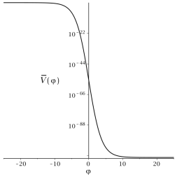
(a) $\bar{V}(\varphi)$ for an EC model.

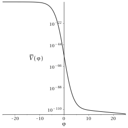
(b) $\bar{V}(\varphi)$ for an ET model.

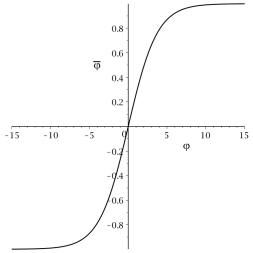
(c) $\bar{\varphi}(\varphi)$

Figure 1: Graphs $\bar{V}(\varphi)=V(\varphi)/V_{-}$ for the EC and ET models and a graph $\bar{\varphi}(\varphi)$, with $\alpha=\frac{7}{3}$ and $\nu=128$. Note that these figures illustrate that the potential plateaus occur when $|\bar{\varphi}|$ is very close to one.

Expressed in $\bar{\varphi}$, the $V_{-}$-normalized potential $\bar{V}(\bar{\varphi})$, $V_{+}$, and the associated $\lambda(\bar{\varphi})=-V_{,\varphi}/V=-\bar{V}_{,\varphi}/\bar{V}$, for the EC and ET examples are given by:

$$\text{EC}\!:\quad\bar{V} =e^{-\nu(1+\bar{\varphi})}, \qquad V_{+} =e^{-2\nu}V_{-}, \qquad\lambda =\frac{\nu}{\sqrt{6\alpha}}\left(1-\bar{\varphi}^{2}\right),$$ (16a)

$$\text{ET}\!:\quad\bar{V} =\frac{e^{-\nu(1+\bar{\varphi})}-e^{-2\nu}}{1-e^{-2\nu}}, \qquad V_{+} =0, \qquad\lambda =\frac{\nu}{\sqrt{6\alpha}}\left(\frac{1-\bar{\varphi}^{2}}{1-e^{-\nu(1-\bar{\varphi})}}\right),$$ (16b)

Note that, in contrast to $V(\phi)$ and $V(\varphi)$, $\bar{V}(\bar{\varphi})$ is independent of $\alpha$. The function $\lambda(\bar{\varphi})$ for a variety of EC and ET models is illustrated in Figure 2.

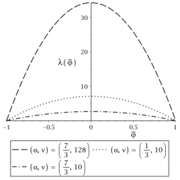
(a) $\lambda(\bar{\varphi})$: EC models.

(b) $\lambda(\bar{\varphi})$: ET models.

Figure 2: Figures (a) and (b) contain graphs $\lambda(\bar{\varphi})$ for the EC and ET models for a variety of values of $\nu$ and $\alpha$. The difference between the EC and ET models for $\bar{\varphi}\leq 0$ is negligible for the present values of $\nu$ since $e^{-\nu}\ll 1$, where $\lambda(\bar{\varphi})$ for $\bar{\varphi}\leq 0$ therefore is governed by $\nu/\sqrt{6\alpha}$; distinguishable differences only occur when $\bar{\varphi}>0$, where $\lambda_{+}=0$ for the EC models while $\lambda_{+}=2/\sqrt{6\alpha}$ in the ET case.

Both $V({\bar{\varphi}})$ and $\lambda({\bar{\varphi}})$ are differentiable (even analytic) when $\bar{\varphi}\in[-1,1]$, where $\lambda_{-}=0$ for the EC and ET models while $\lambda_{+}=0$ for the EC models and $\lambda_{+}=2/\sqrt{6\alpha}$ for the ET models.

As argued in [17], $\alpha\sim{\cal O}(1)$ where, as discussed in e.g. [18], maximal supergravity, string theory, and M-theory suggest that $3\alpha=1,2,3,4,5,6,7$ are particularly interesting, where the choice $\alpha=1$ corresponds to the Starobinski model and Higgs inflation in the Einstein frame. Note also that the recent upper limit of the tensor-to-scalar ratio $r<0.028$ in G. Galloni et al. [40], in combination with relation (4) and the value of the spectral index $n_{s}=0.966$ results in the upper limit $\alpha\lesssim 8$. The large difference between the energy density of the inflationary plateaux and the present dark energy density leads to a much larger value of $\nu$. Based on arguments in [15], one expects $\nu\sim{\cal O}(100)$. In the case of the EC models we can obtain a more precise result: As we will see, the Hubble variable $H$ is monotonically decreasing, while $\lim_{N\rightarrow+\infty}(3H^{2})=V_{+}=e^{-2\nu}V_{-}$, from which it follows that $3H_{0}^{2}>V_{+}=e^{-2\nu}V_{-}$, where $H_{0}$ is the present value of $H$. This in turn yields $\nu>\ln\left(\sqrt{\frac{V_{-}}{3H_{0}^{2}}}\right)$. Using the result in footnote 8 for $V_{-}/3H_{0}^{2}$, which uses $\alpha=\frac{7}{3}$ (the bound is approximately proportional to $\alpha$), results in $\nu>127$. We are henceforth therefore concerned with

$$\alpha\sim{\cal O}(1),\qquad\nu\sim{\cal O}(100),$$ (17)

Note, however, that, $\lambda_{+}$, as will be shown, must satisfy the inequality $\lambda_{+}=2/\sqrt{6\alpha}<\sqrt{2}$ to yield eternal future acceleration, which corresponds to

$$\alpha>\frac{1}{3}.$$ (18)

For illustrative purposes we will typically choose $\alpha=\frac{7}{3}$ and $\nu=128$ as specific examples.

2.2 Field equations and heuristics

Consider a spatially flat FLRW spacetime,

$$ds^{2}=-dt^{2}+a^{2}(t)\delta_{ij}dx^{i}dx^{j},$$ (19)

where $a(t)$ is the cosmological scale factor, and a source consisting of a canonically normalized minimally coupled scalar field, $\varphi$, with a potential $V(\varphi)>0$, and thereby the following energy density and pressure,

$$\rho_{\varphi}=\frac{1}{2}\dot{\varphi}^{2}+V(\varphi),\qquad p_{\varphi}=\frac{1}{2}\dot{\varphi}^{2}-V(\varphi),$$ (20)

and two non-interacting fluids: radiation with $\rho_{\gamma}>0$, $p_{\gamma}=\rho_{\gamma}/3$, and matter with $\rho_{\mathrm{m}}>0$, $p_{\mathrm{m}}=0$.

The definition of the Hubble variable $H$, the (Landau–) Raychaudhuri equation, the Gauss/Hamiltonian constraint (often referred to as the Friedmann equation in FLRW cosmology), the non-linear Klein-Gordon equation, and the energy conservation laws for radiation and matter, are given by

$$\dot{a} =aH,$$ (21a)

$$\dot{H}+H^{2} =-\frac{1}{6}(\rho+3p),$$ (21b)

$$3H^{2} =\rho,$$ (21c)

$$\ddot{\varphi} =-3H\dot{\varphi}-V_{,\varphi},$$ (21d)

$$\dot{\rho}_{\gamma} =-4H\rho_{\gamma},$$ (21e)

$$\dot{\rho}_{\mathrm{m}} =-3H\rho_{\mathrm{m}},$$ (21f)

where an overdot represents the derivative with respect to the cosmic clock time $t$, and where the total energy density $\rho$ and pressure $p$ are given by

$$\rho=\rho_{\varphi}+\rho_{\gamma}+\rho_{\mathrm{m}},\qquad p=p_{\varphi}+\frac{1}{3}\rho_{\gamma}.$$ (22)

Since $\rho>0$ implies that $H^{2}>0$ in (21c), it follows that the Hubble variable $H$ satisfies $H>0$ for expanding models.

Thus, both $\rho_{\gamma}$ and $\rho_{\mathrm{m}}$ monotonically decrease and go to zero toward the future while they blow up asymptotically toward the past. Furthermore, $\rho_{\gamma}/\rho_{\mathrm{m}}$ tends to zero toward the future and infinity toward the past, i.e., radiation dominates over matter toward the past while matter dominates over radiation toward the future. Heuristically, $-3H\dot{\varphi}$ acts as friction in the non-linear Klein-Gordon equation (21d), which makes $\rho_{\varphi}$ decrease, as follows from

$$\dot{\rho}_{\varphi}=-3H(\rho_{\varphi}+p_{\varphi})=-3H\dot{\varphi}^{2}.$$ (23)

Monotonically decreasing inflationary quintessence potentials, $V_{,\varphi}<0$, with an $\alpha$-attractor potential plateaux when $\varphi\rightarrow-\infty$, yield solutions with different asymptotic behaviour in $\varphi$:

• Solutions for which the scalar field originates from $\varphi\rightarrow+\infty$ and then decreases, i.e., $\dot{\varphi}<0$, while decelerating, since then $\ddot{\varphi}>0$; throughout this motion the scalar field energy $\rho_{\varphi}$ is decreasing and hence the scalar field eventually hits the potential and bounces, since $\dot{\varphi}=0$ implies that $\ddot{\varphi}|_{\dot{\varphi}=0}=-V_{,\varphi}>0$, which is followed by that the scalar field increases until $\varphi\rightarrow\infty$.

• Solutions for which the scalar field originates from $\varphi\rightarrow-\infty$ and then forever increases until $\varphi\rightarrow\infty$. Moreover, in the pure scalar field case with $\rho_{\gamma}=\rho_{\mathrm{m}}=0$ there exists a single solution, the inflationary ‘attractor’ solution, for which $\varphi$ is forever increasing until $\varphi\rightarrow\infty$, with an asymptotic origin toward the past at the asymptotic inflationary plateaux, where $\dot{\varphi}=0$ and $\rho_{\varphi}=V_{-}$ when $\varphi\rightarrow-\infty$.

• Solutions for which the scalar field originates from finite values $\varphi_{*}$, which happens when the asymptotic energy density content is dominated by the radiation energy density toward the past, and then increases until $\varphi\rightarrow\infty$.

Cases (ii) and (iii) may not be heuristically clear, but the dynamical systems analysis below shows that this description is correct; moreover, this analysis establishes that cases (i) and (ii) correspond to open sets of solutions while case (iii) corresponds to a set of co-dimension one of solutions. We will also show that the limits $\varphi_{*}$ in case (iii) is intimately connected with the phenomenon of scalar field ‘freezing,’ which plays a significant role for cosmologically viable quintessence solutions.

2.3 Derivation of the dynamical system

To obtain a useful dynamical system, we first define the following quantities

$$\Omega_{\gamma} :=\frac{\rho_{\gamma}}{3H^{2}}, \qquad\qquad\Omega_{\mathrm{m}} :=\frac{\rho_{\mathrm{m}}}{3H^{2}},$$ (24a)

$$\Omega_{\varphi} :=\frac{\rho_{\varphi}}{3H^{2}}, \qquad\qquad\Omega_{V} :=\frac{V}{3H^{2}},$$ (24b)

$$w_{\gamma\mathrm{m}} :=\frac{p_{\gamma}+p_{\mathrm{m}}}{\rho_{\gamma}+\rho_{\mathrm{m}}}=\frac{1}{3}\left(\frac{\rho_{\gamma}}{\rho_{\gamma}+\rho_{\mathrm{m}}}\right), \qquad\qquad w_{\varphi} :=\frac{p_{\varphi}}{\rho_{\varphi}}.$$ (24c)

We then follow [34] and introduce the variables $u$ and $v$ according to

$$u :=\frac{\varphi^{\prime}}{\sqrt{3\Omega_{\varphi}}},$$ (25a)

$$v :=\sqrt{\frac{\Omega_{\varphi}}{3}},$$ (25b)

where a ^′ henceforth denotes the derivative with respect to $e$-fold time

$$N=\ln(a/a_{0}),$$ (26)

where $a_{0}=a(t_{0})$. In agreement with this notation, quantities with values at the present time, $t=t_{0}\Rightarrow N=0$, are denoted by a subscript ₀. The definition (26) implies that $N\rightarrow-\infty$ and $N\rightarrow+\infty$ when $a\rightarrow 0$ and $a\rightarrow\infty$, respectively. We then recall from (9) that we use the following bounded scalar field variable,

$$\bar{\varphi}:=\frac{\phi}{\sqrt{6\alpha}}=\tanh\frac{\varphi}{\sqrt{6\alpha}}.$$ (27)

The final step to obtain our new dynamical system is to change the time variable from the clock time $t$ to the $e$-fold time $N$ by using that

$$\frac{d}{dt}=H\frac{d}{dN},\qquad\frac{d^{2}}{dt^{2}}=H^{2}\left(\frac{d^{2}}{dN^{2}}-(1+q)\frac{d}{dN}\right),$$ (28)

where $q$ is the deceleration parameter, defined by

$$q:=-\frac{a\ddot{a}}{\dot{a}^{2}}=-1-\frac{H^{\prime}}{H}.$$ (29)

Using the above definition for the state vector $(\bar{\varphi},u,v,w_{\gamma\mathrm{m}})$ and the field equations in (21) then leads to:

$$\bar{\varphi}^{\prime} =\frac{3}{\sqrt{6\alpha}}(1-\bar{\varphi}^{2})uv,$$ (30a)

$$u^{\prime} =\frac{3}{2}\left(2-u^{2}\right)\!\left(v\lambda(\bar{\varphi})-u\right),$$ (30b)

$$v^{\prime} =\frac{3}{2}\left(w_{\gamma\mathrm{m}}+1-u^{2}\right)\!\left(1-3v^{2}\right)v,$$ (30c)

$$w_{\gamma\mathrm{m}}^{\prime} =-(1-3w_{\gamma\mathrm{m}})w_{\gamma\mathrm{m}},$$ (30d)

where $\lambda(\bar{\varphi})$ was defined in equation (10). The deceleration parameter $q$ is given by the expression

$$q=-1+\frac{3}{2}\left[3u^{2}v^{2}+(w_{\gamma\mathrm{m}}+1)(1-3v^{2})\right],$$ (31)

as follows from the definition (29) and the Raychaudhuri equation (21b). It is also of interest to define an effective equation of state parameter for the entire matter content

$$w_{\mathrm{eff}}:=\frac{p}{\rho}=w_{\gamma\mathrm{m}}-3(w_{\gamma\mathrm{m}}+1-u^{2})v^{2},$$ (32)

and hence $q=\frac{1}{2}(1+3w_{\mathrm{eff}})$. Note also that it follows that

$$w_{\varphi}=u^{2}-1,\qquad\Omega_{V}=\frac{3}{2}\left(2-u^{2}\right)v^{2},$$ (33)

and hence that it is easy to visualize $w_{\varphi}$ and $\Omega_{\varphi}$ since $w_{\varphi}$ is constant when $u=\mathrm{constant}$ while $\Omega_{\varphi}$ is constant when $v=\mathrm{constant}$, due to the definition (25b).

Once the scalar field potential has been specified, $\lambda(\bar{\varphi})$ follows, which implies that (30) is a closed system of autonomous ordinary differential equations, i.e., a dynamical system.

2.4 State space structure

The state space $(\bar{\varphi},u,v,w_{\gamma\mathrm{m}})$ for quintessential $\alpha$-attractor inflation with a monotonically decreasing potential $V>0$, $\lambda>0$, radiation, $\rho_{\gamma}>0$, and matter, $\rho_{\mathrm{m}}>0$, is determined by the inequalities

$$-1<\bar{\varphi}<1,\qquad-\sqrt{2}<u<\sqrt{2},\qquad 0<v<\frac{1}{\sqrt{3}},\qquad 0<w_{\gamma\mathrm{m}}<\frac{1}{3}.$$ (34)

It follows that the boundaries of the state space are given by

$$\bar{\varphi}=\pm 1,\qquad u=\pm\sqrt{2},\qquad v=0,\qquad v=\frac{1}{\sqrt{3}},\qquad w_{\gamma\mathrm{m}}=0,\qquad w_{\gamma\mathrm{m}}=\frac{1}{3}.$$ (35)

Since $\lambda(\bar{\varphi})$ and its derivatives are non-singular for $\bar{\varphi}\in[-1,1]$, and $\lambda_{-}=0$, $\lambda_{+}$, $\lambda_{\pm}^{(n)}$ thereby exist, this implies that all boundaries are invariant sets. Due to the differentiability assumptions for the potential, the dynamical system (30) is regular everywhere, including on the boundaries (35). This makes it possible to include the 3-dimensional invariant boundary sets and obtain a compact state space. This is highly desirable, since all asymptotics for the solutions for the state vector $(\bar{\varphi},u,v,w_{\gamma\mathrm{m}})$ turn out to reside on these boundaries. We therefore from now on consider the compact state space for which

$$-1\leq\bar{\varphi}\leq 1,\qquad-\sqrt{2}\leq u\leq\sqrt{2},\qquad 0\leq v\leq\frac{1}{\sqrt{3}},\qquad 0\leq w_{\gamma\mathrm{m}}\leq\frac{1}{3},$$ (36)

while the state space defined by the inequalities (34) is referred to as the interior state space.

It is straightforward to show that the deceleration parameter $q$ in (31) satisfies

$$-1\leq q\leq 2.$$ (37)

Here $q=2$ on the invariant boundary subset $v=1/\sqrt{3}$, $u=\pm\sqrt{2}$, which corresponds to $\Omega_{\gamma}=\Omega_{\mathrm{m}}=\Omega_{V}=0$. The lower bound, $q=-1$, which corresponds to a de Sitter state, occurs when $v=1/\sqrt{3}$, $u=0$. This, due to (30b), requires that $\lambda=0$, which is only possible on the $\bar{\varphi}=-1$ boundary, where $\lambda_{-}=0$, and on the $\bar{\varphi}=1$ boundary when $\lambda_{+}=0$, i.e., for the quintessential models with an asymptotically constant potential $V\rightarrow V_{+}>0$ when $\varphi\rightarrow\infty$ ($\bar{\varphi}\rightarrow 1$).

3 General dynamical systems features

The energy conservation of radiation and matter, $\rho_{\gamma}^{\prime}=-4\rho_{\gamma}$, $\rho_{\mathrm{m}}^{\prime}=-3\rho_{\mathrm{m}}$, respectively, yields

$$\rho_{\gamma}=\rho_{\gamma,0}e^{-4N}=3H_{0}^{2}\Omega_{\gamma,0}e^{-4N},\qquad\rho_{\mathrm{m}}=\rho_{\mathrm{m},0}e^{-3N}=3H_{0}^{2}\Omega_{\mathrm{m},0}e^{-3N},$$ (38)

which leads to

$$w_{\gamma\mathrm{m}}=\frac{1}{3}\left(\frac{1}{1+\left(\frac{\Omega_{\mathrm{m},0}}{\Omega_{\gamma,0}}\right)e^{N}}\right).$$ (39)

Thus, as also follows from (30d), $w_{\gamma\mathrm{m}}$ is strictly monotonically decreasing for all interior orbits (i.e., solution trajectories residing in the interior state space), which thereby originate from the invariant radiation boundary $w_{\gamma\mathrm{m}}=1/3$ and end at the invariant matter boundary $w_{\gamma\mathrm{m}}=0$, where the dynamics on these two boundaries are qualitatively similar. In particular, all fixed points are located on the boundaries of these two boundaries, and are, for the presently considered models, given by the same values of $\bar{\varphi},u,v$, see Figure 3.

Next we note that $\bar{\varphi}=\bar{\varphi}_{*}=\mathrm{constant}$ on the invariant $v=0$ ($\Omega_{\varphi}=0$) boundary. Furthermore, the equation for $w_{\gamma\mathrm{m}}$ decouples from those of $\bar{\varphi}$ and $u$ on this boundary, which thereby form a reduced state space $(\bar{\varphi},u)$, which, due to the decoupling of $w_{\gamma\mathrm{m}}$, has a solution space that is identical to that on the invariant $(w_{\gamma\mathrm{m}},v)=(\frac{1}{3},0)$ and $(w_{\gamma\mathrm{m}},v)=(0,0)$ boundaries, see Figure 3. The invariant boundaries $u=\pm\sqrt{2}$ leads to a dynamical system that is independent of the potential, where the scalar field yields the same contribution as a stiff perfect fluid since $w_{\varphi}=u^{2}-1=1$; as a consequence it is not difficult to explicitly solve the equations on these boundaries, as is done in section 5. The features of the solution space of these boundaries are illustrated in Figure 3.

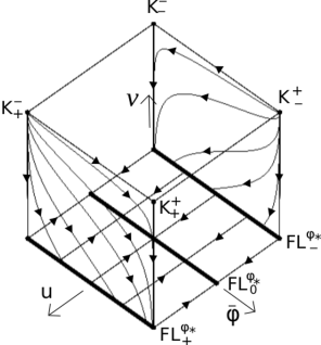
(a) Potential independent boundary structures on the $w_{\gamma\mathrm{m}}=1/3$ state space.

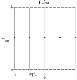
(b) Projection onto $(\bar{\varphi},w_{\gamma\mathrm{m}})$-space of the $v=0$ subset, where $\bar{\varphi}=\bar{\varphi}_{*}=\mathrm{constant}$.

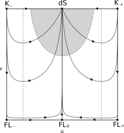
(c) $\lambda=0$.

(d) $0<\lambda\leq\sqrt{2}$.

Figure 3: Figure (a) illustrates the solution space on the potential independent boundaries of the $w_{\gamma\mathrm{m}}=1/3$ boundary (the $w_{\gamma\mathrm{m}}=0$ boundary is similar): $v=0$ ($\Omega_{\varphi}=0$, $\Omega_{\gamma}=1$) results in $\bar{\varphi}=\bar{\varphi}_{*}=\mathrm{constant}$ (and hence that the scalar field $\varphi=\varphi_{*}$ is frozen), while $u=\pm\sqrt{2}$ ($w_{\varphi}=1$; $\Omega_{V}=0$) leads to that $v$ is monotonically decreasing and that $\bar{\varphi}$ is monotonically increasing (decreasing) when $u=\sqrt{2}$ ($u=-\sqrt{2}$). Figure (b) describes a projection onto $(\bar{\varphi},w_{\gamma\mathrm{m}})$-space of the $v=0$ boundary, where $\bar{\varphi}=\bar{\varphi}_{*}=\mathrm{constant}$. Figures (c) and (d) illustrate the solution space structure on the $\bar{\varphi}=\pm 1$ boundaries, where the grey regions correspond to acceleration, i.e. when $q<0$.

Further insights into the dynamics are obtained by noticing that (38) and (39) yields

$$\rho_{\gamma}+\rho_{\mathrm{m}}=3H_{0}^{2}\left(\frac{\Omega_{\mathrm{m},0}^{4}}{\Omega_{\gamma,0}^{3}}\right)\frac{(3w_{\gamma\mathrm{m}})^{3}}{(1-3w_{\gamma\mathrm{m}})^{4}},$$ (40)

which together with the definitions in (24) leads to

$$3H^{2}=\frac{V(\bar{\varphi})}{\Omega_{V}}=\frac{\rho_{\gamma}+\rho_{\mathrm{m}}}{\Omega_{\gamma}+\Omega_{m}}=3H_{0}^{2}\left(\frac{\Omega_{\mathrm{m},0}^{4}}{\Omega_{\gamma,0}^{3}}\right)\frac{(3w_{\gamma\mathrm{m}})^{3}}{(1-3w_{\gamma\mathrm{m}})^{4}(1-3v^{2})}.$$ (41)

Due to (29), which implies $H^{\prime}=-(1+q)H$, and (31), it follows that

$$(3H^{2})^{\prime}=-2(1+q)(3H^{2})=-3\left[3u^{2}v^{2}+(1+w_{\gamma\mathrm{m}})(1-3v^{2})\right](3H^{2}).$$ (42)

Hence, due to that $1+q>0$ (everywhere except at the scalar field boundary where $1+q\geq 0$, which requires special treatment, see section 4), $3H^{2}$, which can be expressed in the state space variables by means of (41), is strictly monotonically decreasing in the interior state space, as well as on the interior radiation and matter boundaries $w_{\gamma\mathrm{m}}=1/3$, $w_{\gamma\mathrm{m}}=0$, respectively. We also note from (30b) that $u$ is monotonically increasing when $u\leq 0$. By taking into account these global features, and the structures on the boundaries, including using the global results concerning the constant and exponential potential boundaries $\bar{\varphi}=\pm 1$ derived in [34], it is not difficult to prove (although for brevity we will refrain from explicitly doing so) that all interior orbits originate from the following fixed points:

• An open set of interior orbits originates from the two ‘kinaton’ (see section 4.2) sources $\mathrm{K}_{-}^{+}$ and $\mathrm{K}_{+}^{-}$ on the radiation boundary with $(\bar{\varphi},u,v,w_{\gamma\mathrm{m}})=(1,-\sqrt{2},1/\sqrt{3},1/3)$ and $(\bar{\varphi},u,v,w_{\gamma\mathrm{m}})=(-1,\sqrt{2},1/\sqrt{3},1/3)$, respectively. The orbits originating from $\mathrm{K}_{-}^{+}$ correspond to solutions for which $\varphi\rightarrow\infty$ toward the past (case (i) in section 2.2) while the orbits coming from $\mathrm{K}_{+}^{-}$ corresponds to solutions for which $\varphi\rightarrow-\infty$ toward the past (case (ii) in section 2.2).

• A set of co-dimension one of orbits originates from the line of fixed points $\mathrm{FL_{0}^{\varphi_{*}}}$ on the radiation boundary with $(\bar{\varphi},u,v,w_{\gamma\mathrm{m}})=(\bar{\varphi}_{*},0,1/\sqrt{3},1/3)$ (case (iii) in section 2.2).

• All interior orbits end at the fixed point $\mathrm{dS}^{+}$ ($\mathrm{P}^{+}$) on the matter boundary with $(\bar{\varphi},u,v,w_{\gamma\mathrm{m}})=(1,0,1/\sqrt{3},0)$ when $\lambda_{+}=0$ ($(\bar{\varphi},u,v,w_{\gamma\mathrm{m}})=(1,\lambda_{+}/\sqrt{3},1/\sqrt{3},0)$ when $0<\lambda_{+}<\sqrt{2}$).

In the next section we will show that there is a single orbit on the scalar field boundary, $v=1/\sqrt{3}$ ($\Omega_{\varphi}=1$, where there thereby is no radiation and matter content), that originates from a de Sitter fixed point on this boundary, and that this orbit corresponds to a solution that belongs to case (ii) in section 2.2. Finally we note that all interior orbits, including those on the scalar field boundary, are heteroclinic orbits (i.e solution trajectories that originate and end at two different fixed points) that end at $\mathrm{dS}^{+}$ ($\mathrm{P}$) when $\lambda_{+}=0$ ($0<\lambda_{+}<\sqrt{2}$).

We conclude this section by noticing that the first and last equalities in (41) yield the following integral

$$\frac{V_{-}}{3H_{0}^{2}}=\frac{3}{2}\left(\frac{\Omega_{\mathrm{m},0}^{4}}{\Omega_{\gamma,0}^{3}}\right)\frac{(3w_{\gamma\mathrm{m}})^{3}(2-u^{2})v^{2}}{(1-3w_{\gamma\mathrm{m}})^{4}(1-3v^{2})\bar{V}(\bar{\varphi})},$$ (43)

which thereby foliates the 4-dimensional interior state space into 3-dimensional invariant subsets, parametrized by $\frac{V_{-}\Omega_{\gamma,0}^{3}}{3H_{0}^{2}\Omega_{\mathrm{m},0}^{4}}$.

4 The scalar field boundary and inflation

4.1 The scalar field boundary

As will be shown, inflation is associated with that an open set of interior orbits in the full state space intermediately closely shadow a special orbit, the inflationary ‘attractor solution,’ on the invariant scalar field boundary $v=1/\sqrt{3}$ during the radiation epoch. The scalar field boundary corresponds to setting $\rho_{\gamma}=\rho_{\mathrm{m}}=0$ ($\Omega_{\gamma}=\Omega_{\mathrm{m}}=0$; $\Omega_{\varphi}=1$), which leads to that the differential equation for $w_{\gamma\mathrm{m}}$ decouples from those of $\bar{\varphi}$ and $u$, where $w_{\gamma\mathrm{m}}$ can be regarded as a test field on a pure scalar field background. However, since inflation takes place deep in the radiation epoch, it is the vicinity of the intersection of the radiation and scalar field boundaries, $w_{\gamma\mathrm{m}}=1/3$ and $v=1/\sqrt{3}$, that is relevant when situating inflation in the full state space. As a consequence the essentials of inflation are connected with the state space $(\bar{\varphi},u)$ and dynamics determined by the following 2-dimensional dynamical system, obtained by setting $v=1/\sqrt{3}$ in (30):

$$\bar{\varphi}^{\prime} =\frac{1}{\sqrt{2\alpha}}(1-\bar{\varphi}^{2})u,$$ (44a)

$$u^{\prime} =\frac{3}{2}\left(2-u^{2}\right)\!\left(\frac{\lambda(\bar{\varphi})}{\sqrt{3}}-u\right).$$ (44b)

The state vector $(\bar{\varphi},u)$ has boundaries given by $\bar{\varphi}=\pm 1$ and $u=\pm\sqrt{2}$. Since

$$q=-1+\frac{3}{2}u^{2},\qquad\epsilon=1+q=\frac{3}{2}u^{2},$$ (45)

for this case due to (31), where $\epsilon$ is the Hubble slow-roll parameter in an inflationary context, the boundaries $u=\pm\sqrt{2}$, which correspond to setting $w_{\varphi}=1$ and $\Omega_{V}=0$ (and thereby $V=0$), result in $q=2$, $\epsilon=1$. As a consequence $H^{\prime}=-(1+q)H=-3H\Rightarrow 3H^{2}=\rho=\rho_{\varphi}=3H_{0}^{2}\exp(-6N)=3H_{0}^{2}(a_{0}/a)^{6}$, which characterizes kinaton evolution (a nomenclature introduced in [41]), i.e., $u=\pm\sqrt{2}$ on the $v=1/\sqrt{3}$ ($\Omega_{\gamma}=\Omega_{\mathrm{m}}=0$) boundary yields the kinaton boundary.

Using (41) and inserting $v=1/\sqrt{3}$ into (33) yields

$$3H^{2}=\frac{V(\bar{\varphi})}{\Omega_{V}}=\frac{V(\bar{\varphi})}{1-\frac{1}{2}u^{2}},$$ (46)

while $H^{\prime}=-(1+q)H$ in combination with (45) results in

$$(3H^{2})^{\prime}=-3u^{2}(3H^{2}),\quad(3H^{2})^{\prime\prime}|_{u=0}=0,\quad(3H^{2})^{\prime\prime\prime}|_{u=0}=-18\lambda^{2}(\bar{\varphi})(3H^{2}).$$ (47)

Thus, for the interior state space of the present boundary $3H^{2}=\frac{V(\bar{\varphi})}{1-\frac{1}{2}u^{2}}$ is monotonically decreasing when $u\neq 0$, and since $\lambda(\bar{\varphi})>0$ when $\bar{\varphi}\in(-1,1)$ it follows from (47) that $3H^{2}=\frac{V(\bar{\varphi})}{1-\frac{1}{2}u^{2}}$ only goes through an inflection point when $u=0$, which can only happen once since $u^{\prime}|_{u=0}>0$. Due to this, the asymptotics of all interior orbits reside on the boundaries $\bar{\varphi}=\pm 1$, $u=\pm\sqrt{2}$, but since $\bar{\varphi}^{\prime}|_{u=\pm\sqrt{2}}=\pm\frac{1}{\sqrt{\alpha}}(1-\bar{\varphi}^{2})$, and since the dynamics on $\bar{\varphi}=\pm 1$ are easily obtained, it follows that all interior orbits in the state space $(\bar{\varphi},u)$ are heteroclinic orbits that asymptotically originate and end at fixed points on the $\bar{\varphi}=\mp 1$ boundaries. There are 6 fixed points on these boundaries in the state space $(\bar{\varphi},u)$:

• Four of these are at the corners of the state space, the ‘kinaton’ fixed points with $q=2$ ($w_{\varphi}=1$), $\mathrm{K}_{-}^{-}$, $\mathrm{K}_{-}^{+}$, $\mathrm{K}_{+}^{-}$, $\mathrm{K}_{+}^{+}$, where superscripts (subscripts) denote the signs of the values of $\bar{\varphi}$ ($u$), e.g., $\mathrm{K}_{-}^{+}$ corresponds to $(\bar{\varphi},u)=(+1,-\sqrt{2})$. The fixed points $\mathrm{K}_{-}^{+}$ and $\mathrm{K}_{+}^{-}$ are hyperbolic sources, while $\mathrm{K}_{-}^{-}$ and $\mathrm{K}_{+}^{+}$ are hyperbolic saddles.

• There is a de Sitter fixed point $\mathrm{dS}^{-}$ at $(\bar{\varphi},u)=(-1,0)$ and an additional one $\mathrm{dS}^{+}$ at $(\bar{\varphi},u)=(+1,0)$ when $\lambda_{+}=0$ (for de Sitter fixed points, $\varphi^{\prime}=0$ and $\Omega_{V}=1$), forming a global sink; if $\lambda_{+}>0$ $\mathrm{dS}^{+}$ is replaced with the global (hyperbolic) sink $\mathrm{P}$ at $(\bar{\varphi},u)=(1,\lambda_{+}/\sqrt{3})$, where this fixed point corresponds to a self-similar power law solution. The condition $\lambda_{+}=2/\sqrt{6\alpha}<\sqrt{2}$, and hence

  $$\alpha>\frac{1}{3},$$ (48)

  leads to that $\mathrm{P}$ results in future eternal acceleration, since this condition yields $q=-1+\lambda_{+}^{2}/2=-1+1/(3\alpha)<0$.

The state space $(\bar{\varphi},u)$ is naturally divided into the regions $u<0$, $u=0$ and $u>0$, where $\bar{\varphi}$ is monotonically decreasing (increasing) when $u<0$ ($u>0$). Since $u^{\prime}>0$ when $u\leq 0$ in the interior state space, where $\lambda(\bar{\varphi})>0$, it follows that the one-parameter set of interior orbits that originates from the source $\mathrm{K}_{-}^{+}$ eventually enters the invariant region $u>0$ where they stay until they, as all interior orbits, end at $\mathrm{dS}^{+}$ or $\mathrm{P}$, depending on if $\lambda_{+}=0$ or $\lambda_{+}=2/\sqrt{6\alpha}<\sqrt{2}$, respectively. These features, taken together with

$$\varphi^{\prime}=\sqrt{3}u,$$ (49)

which is due to (25a) and $\Omega_{\varphi}=1$, show that orbits originating from $\mathrm{K}_{-}^{+}$ belong to case (i) in section 2.2. In contrast, the one-parameter set of orbits originating from the source $\mathrm{K}_{+}^{-}$ and the single heteroclinic separatrix orbit (the inflationary attractor solution, to be discussed below) $\mathrm{dS}^{-}\rightarrow\mathrm{dS}^{+}/\mathrm{P}$ reside completely in the invariant interior subset $u>0$, and hence belong to case (ii) in section 2.2. The solution space is illustrated in Figure 4.

Equation (16) that gives $\lambda(\bar{\varphi})$ for the EC and ET models, illustrated in Figures 2(a) and 2(b), shows that $\lambda_{\mathrm{max}}=\nu/\sqrt{6\alpha}$ at $\bar{\varphi}=0$ for the EC models, which is also close to $\lambda_{\mathrm{max}}$ for the ET models when $\nu$ is large; moreover, the EC and ET models have quite similar $\lambda(\bar{\varphi})$ when $\nu$ is large, until $\bar{\varphi}$ is close to one, due to the limits $\lambda_{+}=0$ and $\lambda_{+}=2/\sqrt{6\alpha}<\sqrt{2}$ in the EC and ET cases, respectively. A large $\nu/\sqrt{6\alpha}$ leads to that $u^{\prime}$ becomes larger than $\bar{\varphi}^{\prime}$ in most of the interior state space, which is the reason why the orbits for such EC and ET models in Figure 4 are characterized by ‘horizontal’ trajectories where $u$ changes much faster than $\bar{\varphi}$.

When $\frac{\nu}{\sqrt{6\alpha}}\gtrsim 3.5$, as for the presently considered models, the heteroclinic separatrix orbit $\mathrm{dS}^{-}\rightarrow\mathrm{dS}^{+}/\mathrm{P}$, and nearby shadowing orbits, exhibit a transient kinaton epoch where they shadow a part of the heteroclinic kinaton orbit $\mathrm{K}_{+}^{-}\rightarrow\mathrm{K}_{+}^{+}$, i.e., the kinaton boundary component with $u=\sqrt{2}$ where $\bar{\varphi}$, and $\varphi$, is increasing. This epoch starts earlier at a smaller $\bar{\varphi}$ and ends later at a larger $\bar{\varphi}$, and is more pronounced, when $\nu/\sqrt{6\alpha}$ increases, as illustrated in Figure 4.

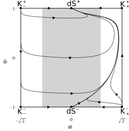
(a) EC: $\alpha=\frac{7}{3}$, $\nu=10$.

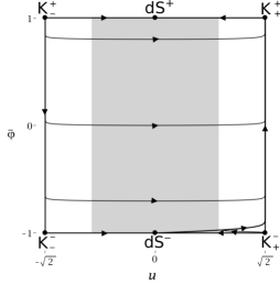
(b) EC: $\alpha=\frac{7}{3}$, $\nu=128$.

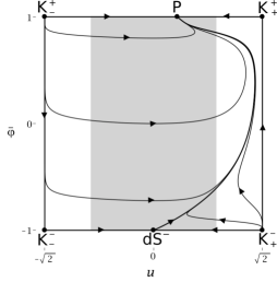
(c) ET: $\alpha=\frac{7}{3}$, $\nu=10$.

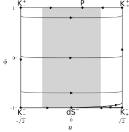
(d) ET: $\alpha=\frac{7}{3}$, $\nu=128$.

Figure 4: Examples of orbits on the $\Omega_{\gamma}=\Omega_{\mathrm{m}}=0$; $\Omega_{\varphi}=1$, $v=1/\sqrt{3}$ scalar field boundary for the EC and ET models, with $\alpha=\frac{7}{3}$ and $\nu=10$, $\nu=128$, including the center manifold orbit (the inflationary ‘attractor’ solution) originating from $\mathrm{dS}^{-}$. The grey regions correspond to acceleration, i.e., $q<0$. As illustrated, the center manifold orbit for the EC and ET models exhibits a kinaton phase with $w_{\varphi}\approx 1$, i.e., a period when it shadows the boundary $u=\sqrt{2}$, when $\frac{\nu}{\sqrt{6\alpha}}\gtrsim 3.5$, which holds for the presently considered range of values for $\alpha$ and $\nu$.

Inflationary descriptions are intimately connected with the slow-roll approximation and slow-roll expansions. We will therefore briefly review this topic and show how it is connected with the present dynamical systems approach and the center manifold analysis of the de Sitter fixed point $\mathrm{dS}^{-}$.

4.2 Slow-roll expansions

The slow-roll approximation is based on the assumptions (see e.g. [42, 43, 44])

$$\dot{\varphi}^{2} <V(\varphi),$$ (50a)

$$\dot{\varphi} \approx-\frac{V_{,\varphi}}{3H},$$ (50b)

$$\epsilon_{V} :=\frac{1}{2}\lambda^{2}\ll 1.$$ (50c)

The first condition corresponds to that the kinetic part of the scalar field energy density is dominated by the potential part, which can be expressed as $u^{2}<1$ while the second condition corresponds to $u\approx\lambda/\sqrt{3}$. We then note that at the de Sitter fixed points $\mathrm{dS}^{\pm}$ we have $\lambda=0$, $u=0$ and hence $\Omega_{V}=1$, i.e. these fixed points represent the limit of the slow-roll approximation.

According to [44], the potential slow-roll parameters

$$\epsilon_{V}=\frac{1}{2}\left(\frac{V_{,\varphi}}{V}\right)^{2}=\frac{1}{2}\lambda^{2},\qquad\eta_{V}:=\frac{V_{,\varphi\varphi}}{V}=\lambda^{2}-\lambda_{,\varphi},$$ (51)

can be used to approximate the Hubble slow-roll parameter $\epsilon=1+q$ to second order as follows:

$$\epsilon\approx\epsilon_{V}\left[1-\frac{2}{3}\!\left(2\epsilon_{V}-\eta_{V}\right)\right],$$ (52)

which when expressed in $\lambda$ yields

$$\epsilon\approx\frac{1}{2}\lambda^{2}\left(1-\frac{2}{3}\lambda_{,\varphi}\right).$$ (53)

Since $\epsilon=1+q=\frac{1}{2}(\varphi^{\prime})^{2}$ (we will express things in $\varphi^{\prime}$ as well as in $u$ since $\varphi^{\prime}$ provides a more natural contact with slow-roll approximations while $u$ is needed for connecting with the present state space approach), it follows that

$$\varphi^{\prime}=\sqrt{3}u\approx\lambda\left(1-\frac{1}{3}\lambda_{,\varphi}\right).$$ (54)

Since $2\epsilon_{V}-\eta_{V}=\lambda_{,\varphi}$ needs to be small in order for the slow-roll approximations to be accurate, we can improve the second order slow-roll approximation in (54) by the following $[1,1]_{\varphi^{\prime}}$ Padé slow-roll approximant (see e.g. [45] and [44] for a discussion and references on Padé approximants):

$$\varphi^{\prime}=\sqrt{3}u\approx\frac{\lambda}{1+\frac{1}{3}\lambda_{,\varphi}}.$$ (55)

Let us next Taylor expand (54) at $\bar{\varphi}=-1$ up to second order. To do so we first define

$$x:=1+\bar{\varphi},$$ (56)

and note that

$$\lambda_{,\varphi}=\left(\frac{d\bar{\varphi}}{d\varphi}\right)\lambda_{,\bar{\varphi}}=\frac{1}{\sqrt{6\alpha}}\left(1-\bar{\varphi}^{2}\right)\lambda_{,\bar{\varphi}}=\frac{x}{\sqrt{6\alpha}}\left(2-x\right)\lambda_{,\bar{\varphi}}.$$ (57)

We then introduce

$$\ell_{n}=\lambda^{(n)}_{-}=\left.\frac{d^{n}\lambda}{d\bar{\varphi}^{n}}\right|_{\bar{\varphi}=-1}=\left.\frac{d^{n}\lambda}{d\bar{\varphi}^{n}}\right|_{x=0},$$ (58)

where we use $\ell_{n}$, $n=1,2,3,\dots$ to obtain succinct notation. A Taylor expansion of $\lambda(\bar{\varphi})$ at $\bar{\varphi}=-1$ ($x=0$) thereby yields

$$\lambda(x)=\sum^{+\infty}_{k=1}\frac{\ell_{k}}{k!}x^{k}$$ (59)

(recall that $\lambda_{-}=\lambda(x=0)=0$). Expanding the expression in (54) to second order in $x=1+\bar{\varphi}$ yields the following expressions:

$$\begin{split}\varphi^{\prime}=\sqrt{3}u&\approx\ell_{1}x\left\{1-\left[\left(\frac{2}{3\sqrt{6\alpha}}\right)\ell_{1}-\frac{1}{2}\left(\frac{\ell_{2}}{\ell_{1}}\right)\right]x\right\}\\ &=\ell_{1}(1+\bar{\varphi})\left\{1-\left[\left(\frac{2}{3\sqrt{6\alpha}}\right)\ell_{1}-\frac{1}{2}\left(\frac{\ell_{2}}{\ell_{1}}\right)\right](1+\bar{\varphi})\right\}.\end{split}$$ (60)

To improve the accuracy we can use the above expression to obtain the following $[1,1]_{\varphi^{\prime}}$ Padé approximant:

$$\begin{split}\varphi^{\prime}=\sqrt{3}u&\approx\frac{\ell_{1}x}{1+\left(\frac{2}{3\sqrt{6\alpha}}\ell_{1}-\frac{\ell_{2}}{2\ell_{1}}\right)x}\\ &=\frac{\ell_{1}(1+\bar{\varphi})}{1+\left[\left(\frac{2}{3\sqrt{6\alpha}}\right)\ell_{1}-\frac{1}{2}\left(\frac{\ell_{2}}{\ell_{1}}\right)\right](1+\bar{\varphi})}.\end{split}$$ (61)

Next, we will show that the above slow-roll approximations yield approximations for the center manifold (CM) orbit of $\mathrm{dS}^{-}$ in the present dynamical systems formulation.

4.3 Center manifold analysis of $\mathrm{dS}^{-}$

Linearizing the dynamical system (44) around $\mathrm{dS}^{-}$ at $(\bar{\varphi},u)=(-1,0)$ yields the tangent spaces

$$E^{s} =\{(\bar{\varphi},u)|\,1+\bar{\varphi}=0\},$$ (62a)

$$E^{c} =\left\{(\bar{\varphi},u)|\,\sqrt{3}u-(1+\bar{\varphi})\ell_{1}=0\right\}.$$ (62b)

Adapting the variables to the center manifold,

$$x:=1+\bar{\varphi},\qquad y:=\sqrt{3}u-\ell_{1}x,$$ (63)

results in that (44) yields the dynamical system

$$x^{\prime} =\frac{1}{\sqrt{6\alpha}}(2-x)x(y+\ell_{1}x),$$ (64a)

$$y^{\prime} =\frac{1}{2}\left[6-(y+\ell_{1}x)^{2}\right](\lambda(x)-y-\ell_{1}x)-\ell_{1}x^{\prime}.$$ (64b)

The center manifold $W^{c}$ is obtained as the graph $y=h(x)$ near $(y,x)=(0,0)$ (i.e., use $x$ as an independent variable), where $h(0)=0$ (fixed point condition) and $\left.\frac{dh}{dx}\right|_{x=0}=0$ (tangency condition). Inserting $y=h(x)$ into (64) and using $x$ as the independent variable leads to

$$\begin{split}&\frac{1}{\sqrt{6\alpha}}(2-x)x\left(h(x)+\ell_{1}x\right)\left(\frac{dh}{dx}+\ell_{1}\right)\\ &\quad-\frac{1}{2}\left[6-(h(x)+\ell_{1}x)^{2}\right](\lambda(x)-h(x)-\ell_{1}x)=0.\end{split}$$ (65)

This equation can be solved approximately by representing $h(x)$ as the formal power series

$$h(x)=\sum_{i=2}^{n}a_{i}x^{i}+{\cal O}(x^{n+1})\qquad\text{as}\qquad x\rightarrow 0,$$ (66)

and by using the Taylor series (59) of $\lambda(x)$. Inserting these series expansions into (65) and solving algebraically for the coefficients $a_{i}$ results in

$$\begin{split}\varphi^{\prime}&=\sqrt{3}u\approx\ell_{1}x\left\{1-\left[\left(\frac{2}{3\sqrt{6\alpha}}\right)\ell_{1}-\frac{1}{2}\left(\frac{\ell_{2}}{\ell_{1}}\right)\right]x\right\},\end{split}$$ (67)

which is the same expression as in (60), obtained by an asymptotic expansion of the slow-roll expansion up to second order, i.e. taking the slow-roll expansion and expanding it in the regime where it is expected to be asymptotically exact, i.e. at the de Sitter fixed point $\mathrm{dS}^{-}$, yields the same result as the center manifold analysis. Note, however, that the slow-roll approximations, which involve $\lambda(x)$, are not the same approximations as the ones that are Taylor expanded in $x$.

Finally, a similar analysis holds for the sink $\mathrm{dS}^{+}$ and leads to closely related results, but where $\mathrm{dS}^{+}$ is a center sink. In this case the expansion also yields an approximation for the analytical center manifold orbit $W^{c}$, but note that all orbits are asymptotically tangential to $E^{c}$ in this case.

The center subspace $W^{c}$ of $\mathrm{dS}^{-}$ thereby corresponds to the separatrix inflationary center manifold (CM) orbit originating from that fixed point, with the tangent $u=(1+\bar{\varphi})\lambda^{(1)}_{-}/\sqrt{3}$ when $\bar{\varphi}\rightarrow-1$ where $\lambda^{(1)}_{-}>0$ for the LC, LT, EC, ET models (see equation (102) in Appendix A). The separatrix CM orbit, originating from $\mathrm{dS}^{-}$, thereby enters the interior state space in the invariant $u>0$ region. In the case of $\lambda_{+}=0$, the center subspace $W^{c}$ of $\mathrm{dS}^{+}$ corresponds to the separatrix orbit originating from $\mathrm{dS}^{-}$ approaching the sink $\mathrm{dS}^{+}$ with the tangent $u=-(1-\bar{\varphi})\lambda^{(1)}_{+}/\sqrt{3}$ when $\bar{\varphi}\rightarrow+1$, where $\lambda^{(1)}_{+}<0$ for the LC and EC models (see equation (103) in Appendix A), where all interior orbits therefore approach $\mathrm{dS}^{+}$ from $u>0$, since they are tangential to $E^{c}$ toward $\mathrm{dS}^{+}$. When $0<\lambda_{+}<\sqrt{2}$ the CM orbit of $\mathrm{dS}^{-}$ is still a separatrix orbit, although in this case it ends at the sink $\mathrm{P}$, for which $u=\lambda_{+}/\sqrt{3}>0$.

The accuracy of the above approximations for the CM orbit are exemplified by a comparison with a numerical calculation of the CM orbit for the EC and ET models with $\alpha=7/3$ and $\nu=128$, given in Figure 5.

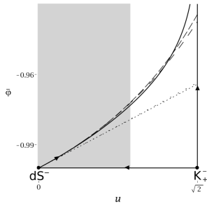
(a) EC: $\alpha=\frac{7}{3}$, $\nu=128$.

(b) ET: $\alpha=\frac{7}{3}$, $\nu=128$.

Figure 5: The numerically computed CM orbit is given by the continuous curve; the slow-roll and the 1st order center manifold approximations are given by the almost overlapping space-dotted and dotted curves, respectively, while the slow-roll and CM Padé $[1,1]_{\varphi^{\prime}}$ approximants are represented by the space-dashed and dashed curves, respectively. The grey regions correspond to when $q<0$.

The inflationary center manifold orbit attracts nearby orbits on the $w_{\gamma\mathrm{m}}=1/3$ boundary since the fixed point $\mathrm{dS}^{-}$ has a center saddle structure $E^{s}$, $E^{c}$ at $\mathrm{dS}^{-}$, where the stable manifold $W^{s}$ has co-dimension one on the radiation boundary while the unstable manifold $W^{c}$ is the CM orbit. It is the co-dimension one stable manifold on the radiation boundary in combination with the zero eigenvalue associated with the CM orbit that makes nearby orbits be strongly attracted to it, explaining, from a dynamical systems perspective, why the CM orbit on the $\Omega_{\gamma}=\Omega_{\mathrm{m}}=0$ ($\rho_{\gamma}=\rho_{\mathrm{m}}=0$), $\Omega_{\varphi}=1$ boundary is known as the inflationary attractor solution.

Before considering some aspects concerning horizon crossing and the end of inflation, let us review some restrictions on model parameters motivated by inflationary considerations.

4.4 Parameter restrictions from the inflationary epoch

As discussed earlier, arguments in [16, 17, 18, 15] suggest that $\alpha$ and $\nu$ take values in the range given in equation (17), i.e,

$$\alpha\sim{\cal O}(1),\qquad\nu\sim{\cal O}(100).$$ (68)

By using the slow-roll approximation during the inflationary epoch, Akrami et al. [15] determine the inflationary plateaux value $V_{-}$ of the potential, which according to equation (2.17) in Akrami et al. [15] is given by

$$V_{-}\approx\frac{(12\pi)^{2}\alpha\Delta N{\cal A}_{s}}{(2\Delta N-3\alpha)^{3}},$$ (69)

where ${\cal A}_{s}$ is the amplitude of the power spectrum of primordial scalar perturbations. As follows from equation (2.2) in [15],

$$\Delta N\approx\frac{2}{1-n_{s}}$$ (70)

is the number of $e$-foldings during inflation through the COBE/Planck normalization, where $n_{s}$ is the (primordial scalar tilt) spectral index. Using values based on $\Lambda$CDM, we obtain the following from Table 1 in Akrami et al. [15]:

$${\cal A}_{s}=2.12605\cdot 10^{-9},\qquad n_{s}=0.966.$$ (71)

Inserting these values into (70) and (69) yields

$$V_{-}\approx\frac{6.985919\cdot 10^{-10}\alpha}{(4-0.102\alpha)^{3}},$$ (72)

which for $\alpha=\frac{7}{3}$ results in

$$V_{-}\approx 3.061568\cdot 10^{-10}.$$ (73)

4.5 Horizon crossing and the end of inflation

Inflationary considerations, e.g. in [16], are based on the first order expansion of the slow-roll approximation, i.e. the first order term in equation (67), given by

$$\varphi^{\prime}=\lambda_{-}^{(1)}(1+\bar{\varphi})=\frac{2\nu}{\sqrt{6\alpha}}(1+\bar{\varphi})$$ (74)

for the EC model, which is also used as an approximation for the ET model for which $\lambda_{-}^{(1)}=\frac{2\nu}{\sqrt{6\alpha}(1-e^{-2\nu})}\approx\frac{2\nu}{\sqrt{6\alpha}}$, due to that $\nu\gg 1$. This, in combination with

$$\bar{\varphi}\approx-1+2e^{\frac{2\varphi}{\sqrt{6\alpha}}}$$ (75)

for both the EC and ET models, as follows from (7) and (9), yields

$$\varphi^{\prime}=\frac{4\nu}{\sqrt{6\alpha}}e^{\frac{2\varphi}{\sqrt{6\alpha}}}.$$ (76)

At the end of inflation, i.e. at $q=0$ on the $v=1/\sqrt{3}$ boundary where $u=\sqrt{2/3}$, it follows, since $\varphi^{\prime}=\sqrt{3}u$, that

$$\varphi^{\prime}_{\mathrm{end}}=\sqrt{2}.$$ (77)

Inserting $\varphi^{\prime}_{\mathrm{end}}=\sqrt{2}$ into (74), and also using (75), gives,

$$\bar{\varphi}_{\mathrm{end}}\approx-1+\frac{\sqrt{3\alpha}}{\nu},\qquad\varphi_{\mathrm{end}}\approx-\frac{\sqrt{6\alpha}}{2}\ln{\left(\frac{2\nu}{\sqrt{3\alpha}}\right)}.$$ (78)

Using that $\varphi_{\mathrm{cross}}\ll\varphi_{\mathrm{end}}$ and (76), (75) leads to

$$\begin{split}\Delta N&=N_{\mathrm{end}}-N_{\mathrm{cross}}=\int^{\varphi_{\mathrm{end}}}_{\varphi_{\mathrm{cross}}}\left(\varphi^{\prime}\right)^{-1}d\varphi\\ &\approx\frac{\sqrt{6\alpha}}{4\nu}\int^{\varphi_{\mathrm{end}}}_{\varphi_{\mathrm{cross}}}e^{-\frac{2\varphi}{\sqrt{6\alpha}}}d\varphi\approx\frac{3\alpha}{4\nu}e^{-\frac{2\varphi_{\mathrm{cross}}}{\sqrt{6\alpha}}}\approx\frac{3\alpha}{2\nu}(1+\bar{\varphi}_{\mathrm{cross}})^{-1},\end{split}$$ (79)

which results in the following leading order approximations:

$$\bar{\varphi}_{\mathrm{cross}}\approx-1+\frac{3\alpha}{2\nu\Delta N},\qquad\varphi_{\mathrm{cross}}\approx-\frac{\sqrt{6\alpha}}{2}\ln{\left(\frac{4\nu\Delta N}{3\alpha}\right)},$$ (80)

which together with (74) or, alternatively, (76) yields

$$\varphi^{\prime}_{\mathrm{cross}}\approx\frac{\sqrt{6\alpha}}{2\Delta N}.$$ (81)

Taking $\Delta N=60$ for $\alpha=7/3$ and $\nu=128$ results in that the above equations give $\bar{\varphi}_{\mathrm{end}}\approx-0.979330$, $\varphi_{\mathrm{end}}\approx-8.553845$, and $(\bar{\varphi}_{\mathrm{cross}},\varphi^{\prime}_{\mathrm{cross}})\approx(-0.999544,0.0311805)$, $\varphi_{\mathrm{cross}}\approx-15.951660$. Let us now connect this with our state space description.

To have around $\Delta N=N_{\mathrm{end}}-N_{\mathrm{cross}}\approx 60$ $e$-folds between horizon crossing and the end of inflation at $q=0$ for the CM orbit and for orbits that intermediately shadow the CM orbit during their evolution implies that horizon crossing initial data have to be extremely close to the de Sitter fixed point $\mathrm{dS}^{-}$. For example, a numerical computation for the CM orbit for the EC and ET models with $\alpha=7/3$ and $\nu=128$ results in that $\Delta N=60$ yields $(\bar{\varphi}_{\mathrm{cross}},u_{\mathrm{cross}})\approx(-0.999542,0.018106)$, where $\bar{\varphi}_{\mathrm{cross}}$ and $u_{\mathrm{cross}}$ correspond to $\varphi_{\mathrm{cross}}=-15.678944$ and $\varphi^{\prime}_{\mathrm{cross}}\approx 0.0313613$, respectively, while $q=0$ leads to $u_{\mathrm{end}}=\sqrt{2/3}$ and, numerically, $\bar{\varphi}_{\mathrm{end}}\approx-0.973204$, which corresponds to $\varphi_{\mathrm{end}}\approx-8.04298889$, while $\varphi_{\mathrm{end}}^{\prime}=\sqrt{2}$ (note that the previous results based on the slow-roll approximation are in good agreement with these numerical results).

Finally, one might ask: What is natural with a region of initial data for inflation that is extremely close to the fixed point $\mathrm{dS}^{-}$ on the radiation boundary? To obtain the present variables we have performed a non-canonical transformation, and one might argue that this region should be translated into a phase space region where a symplectic geometry measure can be applied, but should it be for $\phi$, $\varphi$ or $\bar{\varphi}$ and does this matter? For discussions about the naturalness of inflationary data, see, e.g., [46, 47, 48].

5 Connecting the end of inflation with scalar field freezing

Let us now turn to some aspects concerning reheating and connecting the end of inflation with scalar field freezing, which subsequently initiates quintessence evolution, with a focus on the dynamical systems perspective. Setting $q=0$ in (45) to obtain the end of inflation results in $u^{2}=2/3$ and inserting this into (46) leads to

$$H^{2}_{\mathrm{end}}=\frac{1}{2}V(\bar{\varphi}_{\mathrm{end}})=\frac{1}{2}V_{-}\bar{V}(\bar{\varphi}_{\mathrm{end}}).$$ (82)

Using (16a) for the EC models, which also provides an approximation for the present ET models, and (78) then gives

$$H^{2}_{\mathrm{end}}=\frac{1}{2}V_{-}e^{-\nu(1+\bar{\varphi}_{\mathrm{end}})}\approx\frac{1}{2}V_{-}e^{-\sqrt{3\alpha}}.$$ (83)

Inserting (69) into this expression and using (70) leads to

$$H^{2}_{\mathrm{end}}=\frac{(12\pi)^{2}{\cal A}_{s}\alpha e^{-\sqrt{3\alpha}}\Delta N}{2(2\Delta N-3\alpha)^{3}}\approx\frac{(12\pi)^{2}{\cal A}_{s}\alpha e^{-\sqrt{3\alpha}}}{16\Delta N^{2}}=\frac{1}{64}(12\pi)^{2}{\cal A}_{s}\alpha e^{-\sqrt{3\alpha}}(1-n_{s})^{2}$$ (84)

when $\Delta N\gg\alpha$.

Following the reasoning of Dimopoulos and Owen in [16], the least efficient reheating mechanism is gravitational reheating:

$$(\Omega_{\gamma,\mathrm{end}})_{\mathrm{gr}}\lesssim\Omega_{\gamma,\mathrm{end}}\lesssim 1,$$ (85)

where

$$(\Omega_{\gamma,\mathrm{end}})_{\mathrm{gr}}=\frac{q_{*}g_{*,\mathrm{end}}}{(12\pi)^{2}}H^{2}_{\mathrm{end}},$$ (86)

where $q_{*}\sim 1$ is an efficiency factor and $g_{*,\mathrm{end}}={\cal O}(100)$ is the number of effective relativistic degrees of freedom at the energy scale of inflation. Together with (84) this leads to

$$(\Omega_{\gamma,\mathrm{end}})_{\mathrm{gr}}=\frac{1}{64}q_{*}g_{*,\mathrm{end}}{\cal A}_{s}\alpha e^{-\sqrt{3\alpha}}(1-n_{s})^{2}.$$ (87)

Setting $q_{*}=1$, ${\cal A}_{s}=2.12605\cdot 10^{-9}$, $n_{s}=0.966$ gives

$$(\Omega_{\gamma,\mathrm{end}})_{\mathrm{gr}}=3.84g_{*,\mathrm{end}}\,\alpha e^{-\sqrt{3\alpha}}\cdot 10^{-11}.$$ (88)

After some additional arguments concerning reheating, Dimopoulos and Owen [16] turn to when $V(\varphi)\approx 0$ and obtain the following approximation $\varphi_{*}\approx\varphi_{\mathrm{end}}+\sqrt{\frac{2}{3}}[1-\frac{3}{2}\ln(\Omega_{\gamma,\mathrm{end}})]$. Their analysis corresponds to an approximation based on the $w_{\gamma\mathrm{m}}=1/3$, $u=\sqrt{2}$ ($\Omega_{V}=0$ and hence $V=0$, $w_{\varphi}=1$) boundary, which we now turn to from a dynamical systems perspective.

The equations on this boundary are easily solvable, especially if one uses $\varphi$ instead of $\bar{\varphi}$. Let us begin with the case $u=\sqrt{2}$ (the case $u=-\sqrt{2}$ is easily obtained by means of a discrete symmetry, but this is not relevant in the present context) and $w_{\gamma\mathrm{m}}=1/3$, which leads to

$$\varphi^{\prime} =3\sqrt{2}v,$$ (89a)

$$v^{\prime} =-(1-3v^{2})v,$$ (89b)

from which we obtain

$$\frac{dv}{d\varphi}=-\frac{1}{3\sqrt{2}}\left(1-3v^{2}\right).$$ (90)

The solution to this equation is given by

$$\varphi=\varphi_{\mathrm{i}}+\sqrt{\frac{3}{2}}\ln\left[\frac{(1-\sqrt{3}v)(1+\sqrt{3}v_{\mathrm{i}})}{(1-\sqrt{3}v_{\mathrm{i}})(1+\sqrt{3}v)}\right],$$ (91)

where $(\varphi_{\mathrm{i}},v_{\mathrm{i}})$ denotes an initial point, which determines a particular orbit. The limit $v\rightarrow 0$ yields the following freezing value $\varphi_{*}$ for $\varphi$:

$$\varphi_{*}=\lim_{v\rightarrow 0}\varphi=\varphi_{\mathrm{i}}-\sqrt{\frac{3}{2}}\ln\left[\frac{1-\sqrt{3}v_{\mathrm{i}}}{1+\sqrt{3}v_{\mathrm{i}}}\right]=\varphi_{\mathrm{i}}-\sqrt{\frac{3}{2}}\ln\left[\frac{1-\sqrt{1-\Omega_{\gamma,\mathrm{i}}}}{1+\sqrt{1-\Omega_{\gamma,\mathrm{i}}}}\right],$$ (92)

where we have used that $\Omega_{\gamma}=1-\Omega_{\varphi}=1-3v^{2}$ on this boundary (for the orbit structure, see Figure 3(a)). When $\Omega_{\gamma,\mathrm{i}}$ is close to one, the above exact expression yields the following approximation:

$$\varphi_{*}\approx\varphi_{\mathrm{i}}+\sqrt{\frac{3}{2}}\left[2\ln 2-\ln(\Omega_{\gamma,\mathrm{i}})\right].$$ (93)

Setting the initial values to the of inflation values for $\varphi_{\mathrm{i}}=\varphi_{\mathrm{end}}$ and $\Omega_{\gamma,\mathrm{i}}=\Omega_{\gamma,\mathrm{end}}$ yield the following approximate freezing value $\varphi_{*}$:

$$\varphi_{*}\approx\varphi_{\mathrm{end}}+\sqrt{\frac{3}{2}}\left[2\ln 2-\ln(\Omega_{\gamma,\mathrm{end}})\right].$$ (94)

We note that this approximation differs slightly from the less rigorously derived approximation in [16], $\varphi_{*}\approx\varphi_{\mathrm{end}}+\sqrt{\frac{2}{3}}[1-\frac{3}{2}\ln(\Omega_{\gamma,\mathrm{end}})]$, where the difference between the two expressions is given by $\sqrt{\frac{3}{2}}(2\ln 2)-\sqrt{\frac{2}{3}}\approx 0.88$.

It is even possible to give the solution on the $u=\pm\sqrt{2}$ boundaries that include both radiation and matter in terms of a quadrature. We first note that due to (25a)

$$\varphi^{\prime}=\pm\sqrt{6}\sqrt{\frac{\rho_{\varphi}}{3H^{2}}},$$ (95)

which in combination with

$$\rho_{\varphi}=\rho_{\varphi,\mathrm{i}}e^{-6N},\qquad 3H^{2}=\rho_{\varphi,\mathrm{i}}e^{-6N}+\rho_{\gamma,\mathrm{i}}e^{-4N}+\rho_{\mathrm{m},\mathrm{i}}e^{-3N},$$ (96)

where $N$ is the number of $e$-folds from some convenient initial time $t_{\mathrm{i}}$, gives

$$\varphi=\varphi_{\mathrm{i}}\pm\sqrt{6}\int_{0}^{N}(1+r_{\gamma}e^{2\tilde{N}}+r_{\mathrm{m}}e^{3\tilde{N}})^{-1/2}d\tilde{N},$$ (97)

where $r_{\gamma}:=\rho_{\gamma,\mathrm{i}}/\rho_{\varphi,\mathrm{i}}$ and $r_{\mathrm{m}}:=\rho_{\mathrm{m},\mathrm{i}}/\rho_{\varphi,\mathrm{i}}$. Specializing to $\rho_{\mathrm{m},\mathrm{i}}=0$ and hence $r_{\mathrm{m}}=0$ leads to an explicitly solvable integral which can be used to obtain the previous result (91).

6 Inflationary $\alpha$-attractor quintessence evolution

Although arguably unfair, observations and initial data are usually interpreted in the context of the $\Lambda$CDM paradigm, and we will not deviate from this tradition in this paper when exploring cosmologically observationally viable solutions. We will therefore follow [18, 15] and define observationally viable solutions as solutions associated with $\Lambda$CDM compatible initial data and time developments that are fairly close to $\Lambda$CDM during the observable quintessence epoch. Appendix B contains exact relations that are useful for comparisons between models with a scalar field and $\Lambda$CDM.

To find compatibility with observations in the present context, one has to address the problem of simultaneously choosing (i) the inflationary plateaux-normalized potential $\bar{V}(\varphi)$, which yields $\lambda=-V_{,\varphi}/V=-\bar{V}_{,\varphi}/\bar{V}$, where, in the case of the EC and ET models, specification of $\bar{V}(\bar{\varphi})$ entails choosing the parameter $\nu$, as seen from equation (16), (ii) the parameters, $\alpha$, $V_{-}/3H_{0}^{2}$, which, together with $\bar{V}(\bar{\varphi})$, form the present $\alpha$-attractor model space, and (iii) initial data $(\bar{\varphi}_{\mathrm{i}},u_{\mathrm{i}},v_{\mathrm{i}},w_{\mathrm{rm},\mathrm{i}})$ at some initial time $N_{\mathrm{i}}$.

As regards initial data and solution structures we note the following:

• To obtain $\sim 60$ $e$-folds of inflation requires solutions to be extremely close to the $\mathrm{dS}^{-}$ fixed point on the radiation boundary $w_{\gamma\mathrm{m}}=1/3$, as illustrated by the CM orbit (the inflationary attractor solution) which requires, as exemplified by the EC and ET $\alpha=7/3$, $\nu=128$ models, $(\bar{\varphi}_{\mathrm{i}},u_{\mathrm{i}})\approx(-0.999542,0.018106)$ (i.e. $\varphi_{\mathrm{i}}=-15.678944$, $\varphi^{\prime}_{\mathrm{i}}\approx 0.0313613$), where $t_{\mathrm{i}}$ corresponds to $t_{\mathrm{cross}}$.

  Solutions that exhibit $\sim 60$ $e$-folds of inflation and that hence pass extremely close to the $\mathrm{dS}^{-}$ fixed point on the radiation boundary $w_{\gamma\mathrm{m}}=1/3$ then, thanks to the strong attracting properties of the CM orbit, shadow the CM orbit extremely closely, which in turn for models with $\alpha\sim{\cal O}(1)$, $\nu\sim{\cal O}(100)$ leads to intermediate close shadowing of the kinaton orbit $\mathrm{K}_{+}^{-}\rightarrow\mathrm{K}_{+}^{+}$ on the $u=\sqrt{2}$, $\Omega_{\varphi}=1$, $w_{\gamma\mathrm{m}}=1/3$ boundary. Moreover, the CM orbit and the shadowing orbits end at the same fixed point $\mathrm{dS}^{+}$ when $\lambda_{+}=0$ ($\mathrm{P}$ when $0<\lambda_{+}<\sqrt{2}$) on the matter boundary, $w_{\gamma\mathrm{m}}=0$.

• As pointed out in [34], a long radiation and matter dominated epoch requires that orbits come very close to the $v=0$ ($\Omega_{\varphi}=0$) boundary. This epoch, is initiated before primordial nucleosynthesis and lasts until $\rho_{\varphi}$ makes a significant contribution, thereby commencing the quintessence epoch, which is characterized by $\Omega_{\varphi}>0.03$, as suggested in [34] and references therein. Moreover, the radiation and matter dominated pre-quintessence time interval is required to satisfy $\Delta N\approx 25$. In order to have a pre-quintessence epoch with $\Omega_{\varphi}<0.03$ ($v>0.1$,) and a time interval $\Delta N\approx 25$, numerical calculations show that the EC and ET models with $\alpha=\frac{7}{3}$ $\nu=128$ requires $v_{\mathrm{min}}\approx 10^{-8}$ (at $u=1$ with $\Omega_{\varphi,\mathrm{min}}\approx 10^{-15}$), which due to the closeness to the $v=0$ boundary yields an approximately frozen value of $\varphi=\varphi_{*}$.

  The radiation and matter dominated pre-quintessence epoch corresponds to orbits that subsequently shadow quintessence models associated with the unstable manifold of the line of fixed points $\mathrm{FL}_{0}^{\varphi_{*}}$ on the radiation boundary $w_{\gamma\mathrm{m}}=1/3$ at $\varphi=\varphi_{*}$, described below, when $\Omega_{\varphi}\geq 0.03$ and $N\gtrsim-1.5$, cf. [34].

Due to the uncertainties associated with reheating, we follow [18] and divide the evolution in an inflationary period from $N\sim-85$ to the end of inflation at $N\sim-25$, described by the CM orbit, or rather, an open set of orbits that closely shadows it, and then make a temporal jump to $N=-15$ in the radiation dominated epoch, at a freezing value $\varphi=\varphi_{*}$ at the line of fixed points $\mathrm{FL}_{\mathrm{0}}^{{\varphi}_{*}}$ at the $w_{\gamma\mathrm{m}}=1/3$ boundary, i.e. $(\bar{\varphi},u,v,w_{\gamma\mathrm{m}})=(\bar{\varphi}_{*},0,1/\sqrt{3},1/3)$. It is the unstable manifold of this line that yields the quintessence evolution we, as in [15], will now focus on.

As pointed out in [15], one can view the present models as quintessence models, with inflationary motivated parameter ranges, and only consider the quintessence epoch, which is the problem we will now address and situate in the present state space setting. Since the observable quintessence epoch is finite in time, $\varphi$ only increases with a finite amount from $\varphi_{*}$. This makes it more convenient to use $\varphi$ rather than $\bar{\varphi}$ when describing this epoch, although we will use $\bar{\varphi}$ to describe the entire quintessence epoch, which also includes the future $N\in(0,\infty)$.

Next we present a new method for obtaining initial values for quintessence evolution. Quintessence evolution is described by the unstable manifold of $\mathrm{FL}_{0}^{{\varphi}_{*}}$ on the $w_{\gamma\mathrm{m}}=1/3$ radiation boundary. This is due to that quintessence begins when $\Omega_{\gamma}+\Omega_{\mathrm{m}}\approx 1$ in the radiation dominated regime where $\Omega_{\gamma}\gg\Omega_{\mathrm{m}}$, and since each fixed point on $\mathrm{FL}_{0}^{{\varphi}_{*}}$ on the $w_{\gamma\mathrm{m}}=1/3$ boundary state space ($\bar{\varphi},u,v$) has a single positive eigenvalue, corresponding to the unstable manifold of each fixed point of $\mathrm{FL}_{0}^{{\varphi}_{*}}$, a single zero eigenvalue corresponding to the line of fixed points, and one negative eigenvalue. As a consequence orbits near $\mathrm{FL}_{0}^{{\varphi}_{*}}$ are pushed toward the orbits of the unstable manifold which they thereafter shadow. Due to this, the quintessence evolution of the shadowing orbits are approximately described by the unstable $\mathrm{FL}_{0}^{{\varphi}_{*}}$ orbits, which form the ‘unstable quintessence attractor submanifold’. Note, however, that the attracting property toward the unstable manifold orbits is not as strong as that of the CM orbit, which is due to that the eigenvalue associated with the unstable quintessence attractor manifold is positive while that for the CM orbit is zero.

The future development of an orbit on the unstable manifold of the line of fixed points $\mathrm{FL}_{0}^{{\varphi}_{*}}$ on the $w_{\gamma\mathrm{m}}=1/3$ boundary is obtained by picking a point on the unstable manifold, or very near the unstable manifold, for some initial time $N_{\mathrm{i}}$, which we in agreement with [18] set to $N_{\mathrm{i}}=-15$. However, in contrast to [18, 15], where $\varphi^{\prime}=0$ ($u=0$) is used as an initial value, which yields an orbit that shadows the unstable manifold, and by varying constants in the EC and ET potentials to obtain $H=H_{0}$ at the present time, we use a local analysis of the line of fixed points $\mathrm{FL}^{\varphi_{*}}_{0}$, $(\bar{\varphi},u,v,w_{\gamma\mathrm{m}})=(\bar{\varphi}_{*},0,1/\sqrt{3},1/3)$ in the state space $(\bar{\varphi},u,v,w_{\gamma\mathrm{m}})$, which yields the following initial values

$$\varphi_{\mathrm{i}} \approx\varphi_{*},$$ (98a)

$$u_{\mathrm{i}} \approx\frac{3}{5}\lambda_{*}v_{\mathrm{i}},$$ (98b)

where $\lambda_{*}=\lambda(\varphi_{*})$. Second, we use the exact relation for $w_{\gamma\mathrm{m}}$ in eq. (39) to obtain an initial value for $w_{\gamma\mathrm{m}}$ at $N_{\mathrm{i}}$ connected to the present values $\Omega_{\gamma,0}$, $\Omega_{\mathrm{m},0}$ of $\Omega_{\gamma}$ and $\Omega_{\mathrm{m}}$ (alternatively one can use the linearized version of this equation):

$$(w_{\gamma\mathrm{m}})_{\mathrm{i}}=\frac{1}{3}\left(\frac{1}{1+\left(\frac{\Omega_{\mathrm{m},0}}{\Omega_{\gamma,0}}\right)e^{N_{\mathrm{i}}}}\right).$$ (99)

To connect the unstable $\mathrm{FL}_{0}^{\varphi_{*}}$ orbits from the radiation boundary $w_{\gamma\mathrm{m}}=1/3$ to quintessential $\alpha$-attractor inflation we need to ensure that the values of $V_{-}/3H_{0}^{2}$ are those associated with the inflationary epoch. To do so we can use the integral (43), but is more convenient to do this in the near vicinity of the $\mathrm{FL}_{0}^{\varphi_{*}}$ line of fixed points and use a leading order approximation of this integral, which results in

$$\frac{V_{-}}{3H_{0}^{2}}\approx\frac{3\Omega_{\gamma,0}v_{\mathrm{i}}^{2}e^{-4N_{\mathrm{i}}}}{\bar{V}(\varphi_{*})},$$ (100)

where a given value of $V_{-}/3H_{0}^{2}$ allows one to solve for $v_{\mathrm{i}}$ in terms of a given $\varphi_{*}$. Then $\varphi_{*}$ has to be varied so that $H$, $\Omega_{\gamma}$, $\Omega_{\mathrm{m}}$ obtains their present day values (thanks to the integral and the exact expression for $w_{\gamma\mathrm{m}}$ only one of these variables is independent of the other two).

In Akrami et al. [15] for the $\mathrm{EC}$ and $\mathrm{ET}$ models with $\alpha=7/3$, and $\varphi_{\mathrm{ini}}=10$, they obtained the best fit values of $\nu\approx 127.871$ and $\nu\approx 127.645$ respectively, while we obtain the best fit values $\nu\approx 127.876$ and $\nu\approx 127.650$. This small discrepancy is due to the slightly different initial data. Akrami et al. [15] used $\Omega_{\gamma,0}$, $\Omega_{\mathrm{m},0}$, $\varphi_{*}$, and $\varphi^{\prime}=0$ and hence $u=0$ as their initial data. Strictly speaking, using $u=0$ as initial data is incompatible with the inflationary paradigm since the inflationary attractor solution resides in the $u>0$ region and since the kinaton epoch corresponds to $u\approx+\sqrt{2}$, while models with $u=0$ as initial data originate from $\mathrm{K}^{+}_{-}$ at $(\bar{\varphi},u,v,w_{\gamma\mathrm{m}})=(1,-\sqrt{2},\frac{1}{\sqrt{3}},\frac{1}{3})$. The reason our results and those of Akrami et al. [15] are in such good agreement is due to the attracting nature of the unstable manifold of $\mathrm{FL}_{0}^{\varphi_{*}}$ on the radiation boundary $w_{\gamma\mathrm{m}}=1/3$.

As another example, we now fix $\nu=128$, and keep $\alpha=7/3$. For the $\mathrm{EC}$ and $\mathrm{ET}$ models we obtain the best fit values $\varphi_{*}\approx 9.594$ ($\bar{\varphi}_{*}\approx 0.988$) and $\varphi_{*}\approx 9.214$ ($\bar{\varphi}_{*}\approx 0.986$), respectively. Figures 6 and 7 show the respective orbits in the state space (together with the inflationary attractor CM orbit evolution in $\varphi$ in Figures 6(a) and 7(a)), and the corresponding graphs for $w_{\varphi}$, and $H_{\varphi}/H_{\Lambda}$, where we have used the relevant comparison formulas between $\Lambda$CDM and radiation and the present models given in Appendix B.

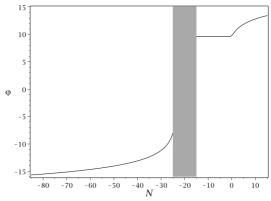
(a) $\mathrm{EC}$ model.

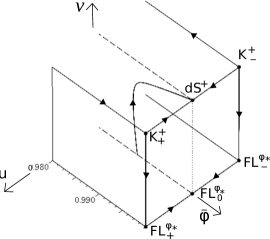
(b) $\mathrm{EC}$ model.

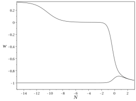
(c) $w_{\varphi}(N)$ and $w_{\mathrm{eff}}(N)$.

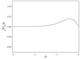
(d) $\frac{H_{\varphi}}{H_{\Lambda}}(N)$.

Figure 6: The EC model with $\alpha=\frac{7}{3}$ and $\nu=128$. Figure (a) depicts the evolution in $\varphi$ during the inflationary and quintessence epochs, for an observationally viable freezing value of $\varphi$. The state space representation of the quintessence epoch of this solution, projected onto $(\bar{\varphi},u,v)$, is depicted in figure (b), while the associated graphs $w_{\varphi}(N)$ (lower curve) and $w_{\mathrm{eff}}(N)$ (upper curve) are shown in figure (c); finally, $\frac{H_{\varphi}}{H_{\Lambda}}(N)$ is shown in figure (d). Note that $w_{\gamma\mathrm{m}}=0$ when $\bar{\varphi}=1$.

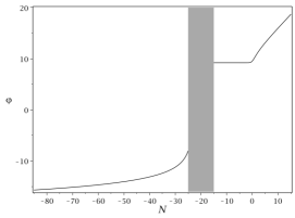
(a) $\mathrm{ET}$ model.

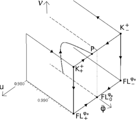
(b) $\mathrm{ET}$ model.

(c) $w_{\varphi}(N)$ and $w_{\mathrm{eff}}(N)$.

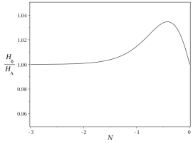
(d) $\frac{H_{\varphi}}{H_{\Lambda}}(N)$.

Figure 7: The ET model with $\alpha=\frac{7}{3}$ and $\nu=128$. Figure (a) depicts the evolution in $\varphi$ during the inflationary and quintessence epochs, for an observationally viable freezing value of $\varphi$. The state space representation of the quintessence epoch of this solution, projected onto $(\bar{\varphi},u,v)$, is depicted in figure (b), while the associated graphs $w_{\varphi}(N)$ (lower curve) and $w_{\mathrm{eff}}(N)$ (upper curve) are shown in figure (c); finally, $\frac{H_{\varphi}}{H_{\Lambda}}(N)$ is shown in figure (d).

7 Discussion

In this paper we have introduced a regular dynamical system for quintessential $\alpha$-attractor inflation on a compact state space. This has the advantage that powerful dynamical systems methods can be applied and this enabled us to obtain (i) a qualitative description of the associated entire solution space and its properties, including asymptotic features, (ii) approximations of solutions, (iii) an analytically based systematic quantitative numerical investigation of the quintessential $\alpha$-attractor EC and ET global solution space structure. For the present models the latter involves two tasks: (a) Connecting orbits to the fixed points from which the physically viable solutions originate and end by varying constants in expressions obtained from local analysis of such fixed points. (b) Identifying the cosmological viable solutions in the global state space.

In particular, this has enabled us to construct a new method for obtaining, in a systematic manner, initial data for viable quintessence evolution. We have also clarified how slow-roll approximations are connected with approximations based on center manifold theory, and in a future paper we will give new accurate and simple approximations for quintessence evolution, using similar dynamical systems based approximation methods as for inflationary evolution, which will further clarify and simplify the identification of observational viable quintessence models and evolution.

Acknowledgments

We thank Yashar Akrami for helpful comments concerning the numerical calculations in [15]. A. A. is supported by FCT/Portugal through CAMGSD, IST-ID, projects UIDB/04459/2020 and UIDP/04459/2020.

Appendix A Asymptotic features for the $\alpha$-attractor inflation potentials

The potentials in (15) for the LC, LT, EC, ET models are characterized by

$$\text{LC}\!:\quad\bar{V} =\frac{1+\nu(1-\bar{\varphi})}{1+2\nu}, \qquad V_{+} =\frac{V_{-}}{1+2\nu}, \qquad\lambda =\frac{\nu}{\sqrt{6\alpha}}\left(\frac{1-\bar{\varphi}^{2}}{1+\nu(1-\bar{\varphi})}\right),$$ (101a)

$$\text{LT}\!:\quad\bar{V} =\frac{1}{2}(1-\bar{\varphi}), \qquad V_{+} =0, \qquad\lambda =\frac{1}{\sqrt{6\alpha}}(1+\bar{\varphi}),$$ (101b)

$$\text{EC}\!:\quad\bar{V} =e^{-\nu(1+\bar{\varphi})}, \qquad V_{+} =e^{-2\nu}V_{-}, \qquad\lambda =\frac{\nu}{\sqrt{6\alpha}}\left(1-\bar{\varphi}^{2}\right),$$ (101c)

$$\text{ET}\!:\quad\bar{V} =\frac{e^{-\nu(1+\bar{\varphi})}-e^{-2\nu}}{1-e^{-2\nu}}, \qquad V_{+} =0, \qquad\lambda =\frac{\nu}{\sqrt{6\alpha}}\left(\frac{1-\bar{\varphi}^{2}}{1-e^{-\nu(1-\bar{\varphi})}}\right),$$ (101d)

when given in $\bar{\varphi}$, which leads to the following asymptotic potential features

$$\text{LC}\!:\quad\lambda^{(1)}_{-} =\frac{2\nu}{\sqrt{6\alpha}(1+2\nu)}, \qquad\lambda^{(2)}_{-} =-\frac{\lambda^{(1)}_{-}}{(1+2\nu)},$$ (102a)

$$\text{LT}\!:\quad\lambda^{(1)}_{-} =\frac{1}{\sqrt{6\alpha}}, \qquad\lambda^{(2)}_{-} =0,$$ (102b)

$$\text{EC}\!:\quad\lambda^{(1)}_{-} =\frac{2\nu}{\sqrt{6\alpha}}, \qquad\lambda^{(2)}_{-} =-\lambda^{(1)}_{-},$$ (102c)

$$\text{ET}\!:\quad\lambda^{(1)}_{-} =\frac{2\nu}{\sqrt{6\alpha}(1-e^{-2\nu})}, \qquad\lambda^{(2)}_{-} =-\left(1-\frac{2\nu e^{-2\nu}}{1-e^{-2\nu}}\right)\lambda^{(1)}_{-},$$ (102d)

and

$$\text{LC}\!:\quad\lambda_{+} =0, \qquad\lambda^{(1)}_{+} =-\frac{2\nu}{\sqrt{6\alpha}}, \qquad\lambda^{(2)}_{+} =(1+2\nu)\lambda^{(1)}_{+},$$ (103a)

$$\text{LT}\!:\quad\lambda_{+} =\frac{2}{\sqrt{6\alpha}}, \qquad\lambda^{(1)}_{+} =\frac{1}{\sqrt{6\alpha}}, \qquad\lambda^{(2)}_{+} =0,$$ (103b)

$$\text{EC}\!:\quad\lambda_{+} =0, \qquad\lambda^{(1)}_{+} =-\frac{2\nu}{\sqrt{6\alpha}}, \qquad\lambda^{(2)}_{+} =\lambda^{(1)}_{+},$$ (103c)

$$\text{ET}\!:\quad\lambda_{+} =\frac{2}{\sqrt{6\alpha}}, \qquad\lambda^{(1)}_{+} =\frac{1-\nu}{\sqrt{6\alpha}}, \qquad\lambda^{(2)}_{+} =-\frac{(1-\frac{\nu}{3})\nu}{\sqrt{6\alpha}}.$$ (103d)

Appendix B Exact relations and $\Lambda$CDM comparisons

In order to compare a scalar field model with the $\Lambda$CDM model we, for simplicity, identify the models at the present time as regards the rate of expansion and the matter content. Specifically we require that

$$H_{\varphi,0}=H_{\Lambda,0}=H_{0},\qquad\Omega_{\Lambda,0}=\Omega_{\varphi,0}=1-\Omega_{\gamma,0}-\Omega_{m,0},$$ (104)

where $\Omega_{\Lambda,0}:=\Lambda/3H_{0}^{2}$, while $H_{0}$, $\Omega_{\gamma,0}$ and $\Omega_{m,0}$ are the observed Hubble parameter and the dimensionless Hubble-normalized radiation and matter densities at the present time. Common for scalar field models and $\Lambda$CDM with radiation is also $\rho_{\gamma}=3H_{0}^{2}\Omega_{\gamma,0}e^{-4N}$, $\rho_{\mathrm{m}}=3H_{0}^{2}\Omega_{\mathrm{m},0}e^{-3N}$ and hence

$$w_{\gamma\mathrm{m}}=\frac{1}{3}\left(\frac{1}{1+\left(\frac{\Omega_{\mathrm{m,0}}}{\Omega_{\gamma,0}}\right)e^{N}}\right).$$ (105)

We then define

$$E_{\varphi}(N):=\frac{H_{\varphi}(N)}{H_{0}},\qquad E_{\Lambda}(N):=\frac{H_{\Lambda}(N)}{H_{0}},$$ (106)

and note that

$$E_{\varphi}^{2}=\frac{\Omega_{\gamma,0}e^{-4N}+\Omega_{\mathrm{m},0}e^{-3N}}{1-\Omega_{\varphi}},\qquad E_{\Lambda}^{2}=\Omega_{\gamma,0}e^{-4N}+\Omega_{\mathrm{m},0}e^{-3N}+\Omega_{\Lambda,0},$$ (107)

where we recall that $\Omega_{\varphi}=3v^{2}$. Due to eq. (107) it follows that

$$\left(\frac{H_{\varphi}}{H_{\Lambda}}\right)^{2}=\left(\frac{E_{\varphi}}{E_{\Lambda}}\right)^{2}=\frac{\Omega_{\gamma,0}e^{-4N}+\Omega_{\mathrm{m},0}e^{-3N}}{(1-\Omega_{\varphi})(\Omega_{\gamma,0}e^{-4N}+\Omega_{\mathrm{m},0}e^{-3N}+\Omega_{\Lambda,0})}.$$ (108)

To obtain a feeling for the initial value of $N=N_{\mathrm{i}}$, note that

$$N=\ln\left[\left(\frac{\rho_{\mathrm{m}}}{\rho_{\gamma}}\right)\left(\frac{\Omega_{\gamma,0}}{\Omega_{\mathrm{m},0}}\right)\right].$$ (109)

Thus, setting, e.g., $\Omega_{\gamma,0}=10^{-5}$ and $\Omega_{\mathrm{m},0}=0.32$, results in

$$\frac{\rho_{\mathrm{m}}}{\rho_{\gamma}} \in[10^{-2},10^{2}]\quad\Rightarrow\quad N\in[-14.98,-5.77],$$ (110a)

$$\frac{\rho_{\mathrm{m}}}{\rho_{\gamma}} =1\quad\Rightarrow\quad N=N_{\mathrm{eq}}=-10.37.$$ (110b)

The cosmological redshift, $z$, is kinematically determined by

$$z=\frac{a_{0}}{a}-1=e^{-N}-1\qquad\Rightarrow\qquad N=-\ln(1+z).$$ (111)

Thus, e.g., $z=0.4$, $z=1$, $z=1.5$, $z=10$, $z=147.4$, $z=1100$, $z=10^{10}$ correspond to $N=-0.34$, $N=-0.69$, $N=-0.92$, $N=-2.40$, $N=-5.00$, $N=-7.00$, $N=-23.03$, respectively.

References

- [1] A. G. Riess et al. Observational evidence from supernovae for an accelerating universe and a cosmological constant. Astron. J., 116:1009, 1998.
- [2] S. Perlmutter et al. Measurements of omega and lambda from 42 high redshift supernovae. Astron. J., 517:565, 1999.
- [3] Planck Collaboration. Planck 2018 results. VI. cosmological parameters. arXiv:1807.06209 [astro-ph.CO], 2018.
- [4] Planck Collaboration: Y. Akrami et al. Planck 2018 results. x. constraints on inflation. arXiv:1807.06211 [astro-ph.CO], 2018.
- [5] S. Alam et al. The clustering of galaxies in the completed sdss-iii baryon oscillation spectroscopic survey: cosmological analysis of the dr12 galaxy sample. MNRAS, 470:2617, 2017.
- [6] T. M. C. Abbott et al. DES Collaboration. Dark energy survey year 1 results: Cosmological constraints from cluster abundances and weak lensing. Phys. Rev. D, 102:023509, 2020.
- [7] A. G. Riess, S. Casertano, W. Yuan, L. M. Macri, and D. Scolnic. Large magellanic cloud cepheid standards provide a 1% foundation for the determination of the hubble constant and stronger evidence for physics beyond CDM. The Astrophysical Journal, 876(1):85, 2019.
- [8] P. J. E. Peebles and A. Vilenkin. Quintessential inflation. Phys. Rev. D, 59:063505, 1999.
- [9] J. Martin, C. Ringeval, and V. Vennin. Encyclopædia inflationaris. Physics of the Dark Universe, 5:75, 2014.
- [10] M. Galante, R. Kallosh, A. Linde, and D. Roest. Unity of cosmological inflation attractors. Phys. Rev. Lett., 114:141302, 2015.
- [11] R. Kallosh and A. Linde. Escher in the sky. Comptes Rendus Physique, 16:914–927, 2015.
- [12] S. Ferrara and R. Kallosh. Seven-disc manifold -attractors and b modes. Phys. Rev. D, 94:0126015, 2016.
- [13] R. Kallosh, A. Linde, D. Roest, and Y. Yamada. D3 induced geometric inflation. JHEP, 07:057, 2017.
- [14] R. Kallosh, A. Linde, T. Wrase, and Y. Yamada. Maximal supersymmetry and b-mode targets. JHEP, 04:144, 2017.
- [15] Y. Akrami et al. Quintessential -attractor inflation: forecasts for stage iv galaxy surveys. JCAP, 04:006, 2021.
- [16] K. Dimopoulos and C. Owen. Quintessential inflation with -attractors. J. of Cosmology and Astroparticle Physics, 06:027, 2017.
- [17] K. Dimopoulos, L. D. Wood, and C. Owen. Instant preheating in quintessential inflation with -attractors. Phys. Rev. D, 97:063525, Mar 2018.
- [18] Y. Akrami et al. Dark energy, -attractors, and large-scale structure surveys. JCAP, 06:041, 2018.
- [19] R. Kallosh, A. Linde, and D. Roest. Large field inflation and double -attractors. J. High Energ. Phys., 08:052, 2014.
- [20] R. Kallosh and A. Linde. Universality class in conformal inflation. J. of Cosmology and Astroparticle Physics, 2013:1475, 2013.
- [21] J. J. M. Carrasco, R. Kallosh, and A. Linde. Cosmological attractors and initial conditions for inflation. Phys. Rev. D, 92:063519, 2015.
- [22] J. J. M. Carrasco, R. Kallosh, and A. Linde. -attractors: Planck, lhc and dark energy. J. High Energ. Phys., 147, 2015.
- [23] A. Linde. Single-field -attractors. J. of Cosmology and Astroparticle Physics, 2015:003, 2015.
- [24] A. Linde. Gravitational waves and large field inflation. J. of Cosmology and Astroparticle Physics, 2017:006, 2017.
- [25] A. Linde. Random potentials and cosmological attractors. J. of Cosmology and Astroparticle Physics, 2017:028, 2017.
- [26] A.A. Starobinsky. A new type of isotropic cosmological models without singularity. Physics Letters B, 91(1):99–102, 1980.
- [27] John D. Barrow and S. Cotsakis. Inflation and the conformal structure of higher-order gravity theories. Physics Letters B, 214(4):515–518, 1988.
- [28] Fedor Bezrukov and Mikhail Shaposhnikov. The standard model higgs boson as the inflaton. Physics Letters B, 659(3):703–706, 2008.
- [29] A. Alho, C. Uggla, and J. Wainwright. Dynamical systems in perturbative scalar field cosmology. Class. Quantum Grav., 37(22):225011, 2020.
- [30] A. Alho, J. Hell, and C. Uggla. Global dynamics and asymptotics for monomial scalar field potentials and perfect fluids. Class. Quant. Grav., 32(14):145005, 2015.
- [31] A. Alho and C. Uggla. Scalar field deformations of lambda-cdm cosmology. Phys. Rev. D, 92(10):103502, 2015.
- [32] A. Alho and C. Uggla. Inflationary -attractor cosmology: A global dynamical systems perspective. Phys. Rev. D, 95(8):083517, 2017.
- [33] A. Alho, C. Uggla, and J. Wainwright. Perturbations of the lambda-cdm model in a dynamical systems perspective. JCAP, 09:045, 2019.
- [34] A. Alho, C. Uggla, and J. Wainwright. Quintessence in a state space perspective. Physics of the Dark Universe, 39:101146, 2023.
- [35] C. B. Collins. More qualitative cosmology. Comm. Math. Phys., 23(2):137–158, 1971.
- [36] O. I. Bogoyavlenskii and S. P. Novikov. Singularities of the cosmological model of the bianchi ix type according to the qualitative theory of differential equations. JETP, 37(5):747–755, 1973.
- [37] J. Wainwright and G. F. R. Ellis. Dynamical systems in cosmology. Cambridge University Press, 1997.
- [38] A. A. Coley. Dynamical systems and cosmology. Kluwer Academic Publishers, Dordrecht, 2003.
- [39] S. Bahamonde, C. G. Böhmer, S. Carloni, E. J. Copeland, Wei Fang, and N. Tamanini. Dynamical systems applied to cosmology: Dark energy and modified gravity. Physics Reports, 775-777:1–122, 2018.
- [40] Giacomo Galloni, Nicola Bartolo, Sabino Matarrese, Marina Migliaccio, Angelo Ricciardone, and Nicola Vittorio. Updated constraints on amplitude and tilt of the tensor primordial spectrum. Journal of Cosmology and Astroparticle Physics, 2023(04):062, apr 2023.
- [41] Michael Joyce and Tomislav Prokopec. Turning around the sphaleron bound: Electroweak baryogenesis in an alternative post-inflationary cosmology. Phys. Rev. D, 57:6022–6049, 1998.
- [42] P. J. Steinhardt and M. S. Turner. Prescription for successful new inflation. Phys. Rev. D, 29:2162–2171, 1984.
- [43] A. R. Liddle and D. H. Lyth. The cold dark matter density perturbations. Physics Reports, 231:1–105, 1993.
- [44] A. R. Liddle, P. Parsons, and J. D. Barrow. Formalizing the slow-roll approximation in inflation. Phys. Rev. D, 50:7222, 1994.
- [45] A. Alho and C. Uggla. Global dynamics and inflationary center manifold and slow-roll approximants. Journal of Mathematical Physics, 56(012502), 2015.
- [46] G.N. Remmen and S.M. Carroll. Attractor solutions in scalar-field cosmology. Phys. Rev. D, 88:083518, 2013.
- [47] G.N. Remmen and S.M. Carroll. How many e-folds should we expect from high-scale inflation? Phys. Rev. D, 90:063517, 2014.
- [48] R. Grumitt and D. Sloan. Measures in mutlifield inflation, 2016.