Multi-Dimensional Refinement Graph Convolutional Network with Robust Decouple Loss for Fine-Grained Skeleton-Based Action Recognition
Abstract
Graph convolutional networks have been widely used in skeleton-based action recognition. However, existing approaches are limited in fine-grained action recognition due to the similarity of inter-class data. Moreover, the noisy data from pose extraction increases the challenge of fine-grained recognition. In this work, we propose a flexible attention block called Channel-Variable Spatial-Temporal Attention (CVSTA) to enhance the discriminative power of spatial-temporal joints and obtain a more compact intra-class feature distribution. Based on CVSTA, we construct a Multi-Dimensional Refinement Graph Convolutional Network (MDR-GCN), which can improve the discrimination among channel-, joint- and frame-level features for fine-grained actions. Furthermore, we propose a Robust Decouple Loss (RDL), which significantly boosts the effect of the CVSTA and reduces the impact of noise. The proposed method combining MDR-GCN with RDL outperforms the known state-of-the-art skeleton-based approaches on fine-grained datasets, FineGym99 and FSD-10, and also on the coarse dataset NTU-RGB+D X-view version.
Index Terms:
Graph convolutional network, fine-grained action, Robust Decouple loss, Spatial-Temporal attentionI Introduction
Skeleton-based action recognition has been an attractive emerging topic because of its excellent robustness in dynamic environments and human-centered applications. In recent years, fine-grained action tasks are followed with interest in many fields. However, the fine-grained action recognition task remains challenging due to new difficulties.
The first challenge is to explore the discriminative power of spatial-temporal joints. This indicates that inter-joint and inter-frame relationships vary with different actions and their types [1]. Early RNN or CNN methods [2, 3, 4, 5, 6] usually model the skeleton data as a sequence of the coordinate vectors or a pseudo-image but ignore the dependencies between joints. Many frontier GCN-based methods [7, 8, 9, 10, 11, 12, 13] apply graph convolution with fixed and learnable parameter matrices to achieve spatial pattern modeling. However, the previous GCN-based methods lack considering the advantages of both channels and spatial-temporal attention. For multi-modality data, STAR-transformer [14] adopts the method of adding spatial-temporal fusion attention after feature extraction, but for skeletal data, this approach will cause feature redundancy and lead to performance limitations. Efficient-GCN [15] has concentrated on spatial-temporal relationships by modeling a new attention block in fixed channels, which causes a lack of adaptive representation capability of channels and the difficulty of further expansion on the variable channel models. Therefore, the spatial-temporal discriminative capability in the existing models is insufficient for the fine-grained recognition task.
The second challenge is to obtain robust and discriminative embedding sample distributions of skeleton-based actions. For fine-grained recognition tasks, both separable and discriminative learned features should be considered in loss functions[16]. In addition, inevitable outliers and noises also should be noticed. Some existing work [17, 18] offer solutions for noise labels, but the outliers in collected data of joints are still difficult to deal with. The conventional softmax loss mainly encourages the separability of features, which causes weak intra-class compactness even if the model is more advanced. The explicit methods [19, 20] achieve maximized inter-class and minimize intra-class variance (one or both) by utilizing an additional loss. However, existing explicit methods are weak-robust for outliers and numerically unbalanced with softmax loss. Angular softmax approaches [21, 22, 23] solve the problems by normalizing features and class centers in softmax. Some scale and margin versions of angular softmax are also proposed to enhance the discriminative capability of features [24, 25]. These implicit methods are challenging to optimize norms and margins for each class adaptively (the details will be presented in Sec 2.2 and 3.3). Considering the deficiencies in existing loss functions, we need a more effective loss to achieve more robust and discriminative embedding for the fine-grained recognition task.
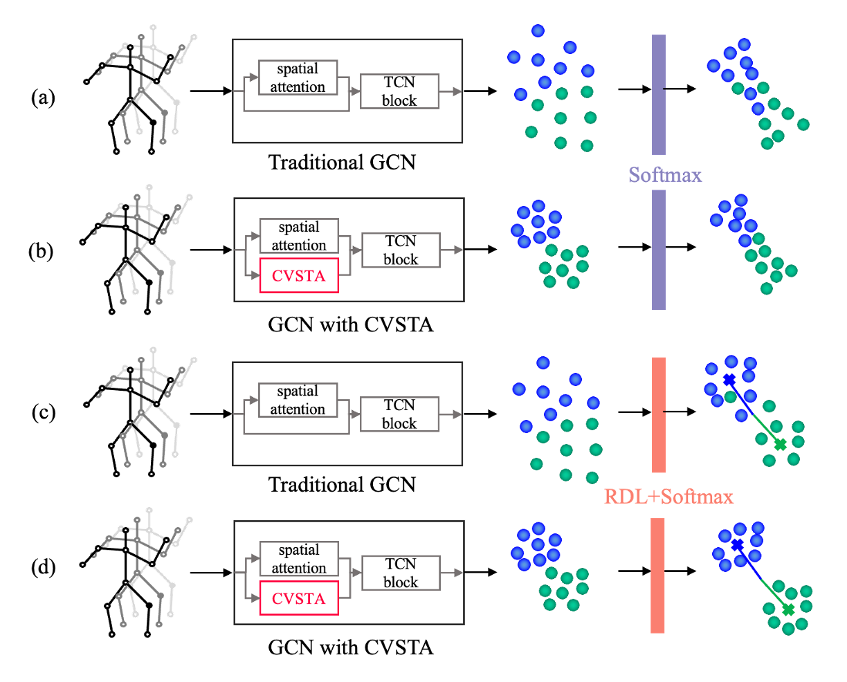
In this paper, we propose a dynamic spatial-temporal attention block called Channel-Variable Spatial-Temporal Attention (CVSTA) to solve the problems above. It can build a comprehensive connection between frames and joints and capture more potential features. Besides, as a flexible block, it could be easily combined with other GCNs to get better performance. In contrast to traditional GCN-based methods, our approach obtains spatial-temporal features more sufficiently, which promotes the clustering of intra-class samples. Therefore, to enhance the discrimination among channel-, joint- and frame-level, we propose a Multi-Dimensional Refinement Graph Convolution Network (MDR-GCN), which includes the channel-wise GCN framework with CVSTA and enhanced temporal convolution blocks.
To fully consider the noises and outliers of skeleton data, motivated by related fine-grained tasks [26, 27], we propose a Robust Decouple Loss (RDL). RDL achieves large class-wise discriminative embedding by leveraging the ratio of norms of each class along with both intra-class and inter-class cosine of the vectors, which significantly improves the robustness of the existing explicit loss function. Thus, RDL can optimize variances along the cosine/norm aspect(s) and reduce the numerical discrepancy of losses, further facilitating the role of CVSTA. Besides, by decoupling center loss [19], RDL has more scales that can adjust the impact of noisy data. Figure 1 shows the improvement in the feature distribution arising from RDL and CVSTA.
Our contributions are summarized as follows:
1. We propose a new GCN model named MDR-GCN for fine-grained action recognition by utilizing our designed CVSTA block, which captures relationships of joints across frames in variable channels.
2. We propose RDL by decoupling the center loss for robust discriminative embedding. In our experiments, RDL enhances the performance of CVSTA and outperforms state-of-the-art losses.
3. The proposed method combining MDR-GCN with RDL outperforms the known state-of-the-art skeleton-based approaches on the FineGym99, the FSD-10, and the NTU-RGB+D datasets.
II Related Work
II-A Skeleton-based action recognition
Early skeleton-based action recognition methods mainly employ RNN or CNN to extract discriminative features. RNN-based approaches [2, 4, 28, 29] generally explain action features as multi-dimensional time series, focusing on extracting actions’ temporal features rather than exploiting spatial ones. To deeply realize spatial characteristics, CNN-based networks [30, 5, 31, 32, 33, 34] transform the skeleton data into grid images to simplify the training process. However, neither of the two approaches can model the structured dependencies of skeletons because of the inherent calculation strategy.
In recent years, researchers have become increasingly interested in GCN-based methods [35, 36, 37, 38, 39] which can reflect the structured relationships between skeletons. Most studies have focused on spatial modeling, which contains pre-defined [7], learnable [8], and dynamic [11] ways. ST-GCN [7] utilizes the original heuristically pre-defined graph physically driven by the human body, which hardly realizes the dependencies between unlinked joints. As a learnable method, 2S-AGCN [8] is further proposed to capture data-driven graphs for more dependencies of skeletons in shared channels. To explore more types of motion features in channel view, some researchers suggested dynamic independent channel-based models [40, 11] by offering more graph topologies along with channels. DC-GCN [40] sets individually parameterized topologies for different channel groups, but it is hard to optimize because of excessive parameters. Integrating the shared and learnable channel-wise topologies is a practical scheme. CTR-GCN [11] leverages skeleton attention to refine channels and spatial features and considers the balance between learning capability and parameter quantity. InfoGCN [13] emphasizes the importance of paying attention to the intrinsic connection of joints, indicating that GC using only external topology will lead to serious inefficiency and information loss in message transmission. Nevertheless, spatial-temporal information on joints in different frames is not yet considered in the above work. FD-GCN [10] offers a Focusing-Diffusion Graph Convolutional structure to achieve spatial-temporal attention, but the approach ignores differences among channels, which causes information redundancy. A spatial-temporal attention module is proposed in EfficientGCN [15] to represent action-specific correlations with fewer parameters. However, compared with CTR-GCN or InfoGCN, the limited performance and scalability of channel-fixed attention weaken the discriminative power in the channel view.
The 3D CNN-based methods are also a hot spot in the skeleton-based action recognition task. PoseC3D [41] uses the 3D CNN instead of graph convolution, but the heatmap of the input takes up more memory. Besides, compared with the newer GCN method, the 3D CNN-based methods have not achieved a significant performance advantage but occupy more parameters [11]. Therefore, the GCN-based methods are still competitive when the above problems are solved.
II-B Loss functions for fine-grained tasks
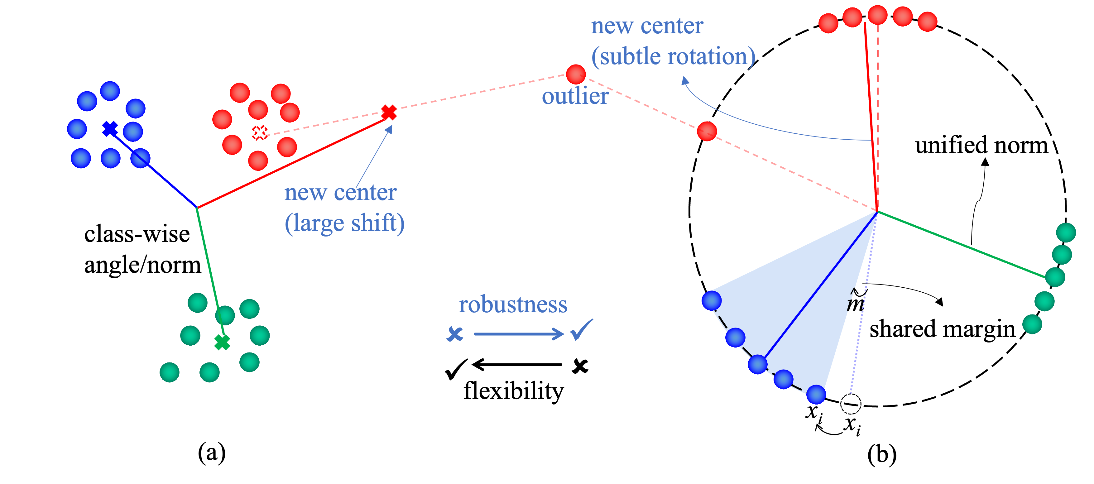
In recent years, researchers have realized that the softmax loss lacks the capability of learning discriminative embedding for fine-grained classification [42, 43]. Existing embedding losses fall into two major categories: explicit and implicit ones. Figure 2 shows the characteristics of the two kinds of losses. (a) Early explicit methods [44, 45, 46, 47] commonly employ siamese networks with lots of parameters to get faithful discriminative embedding. To fully utilize class annotation, some later supervised embedding losses are proposed by attaching to a classification loss. As a classical method, Center loss [19] is frequently used for fine-grained classification by enhancing the discriminant power in the loss layer of networks. Nevertheless, the discriminative embedding in the Euclidean space of the above approaches always suffers from the value imbalance between the center loss version and cross-entropy-based loss, in addition to weak robustness by outliers or complex feature distributions. (b) To relieve the above issues, the angular-margin-based approach [21, 48, 22, 23, 24] may be the better choice, which aims to expand the angle interval of classes to realize the optimization. Sphereface [22] leverages multiplying marginal parameters by the intra-class angle to realize the implicit embedding loss. For feasible optimization, the following methods [49, 24] involve an additional angular margin to accelerate the training process. However, the empirically scalable and marginal hyperparameters limit the discriminant capability of implicit loss. Recent methods [50, 51, 27] employ adaptive hyperparameters to improve the robustness. However, all these implicit methods have not noticed the class-wise discriminant on both angular and norm-based aspects, especially for large intra-class and slight inter-class variance of samples. Compared with (a), our method measures the features through the angle and norm scale, so we have more adjustment space to achieve the same optimization goal as (a) while reducing the deviation of the center’s abnormal point and maintaining the advantage of flexibility.
III Method
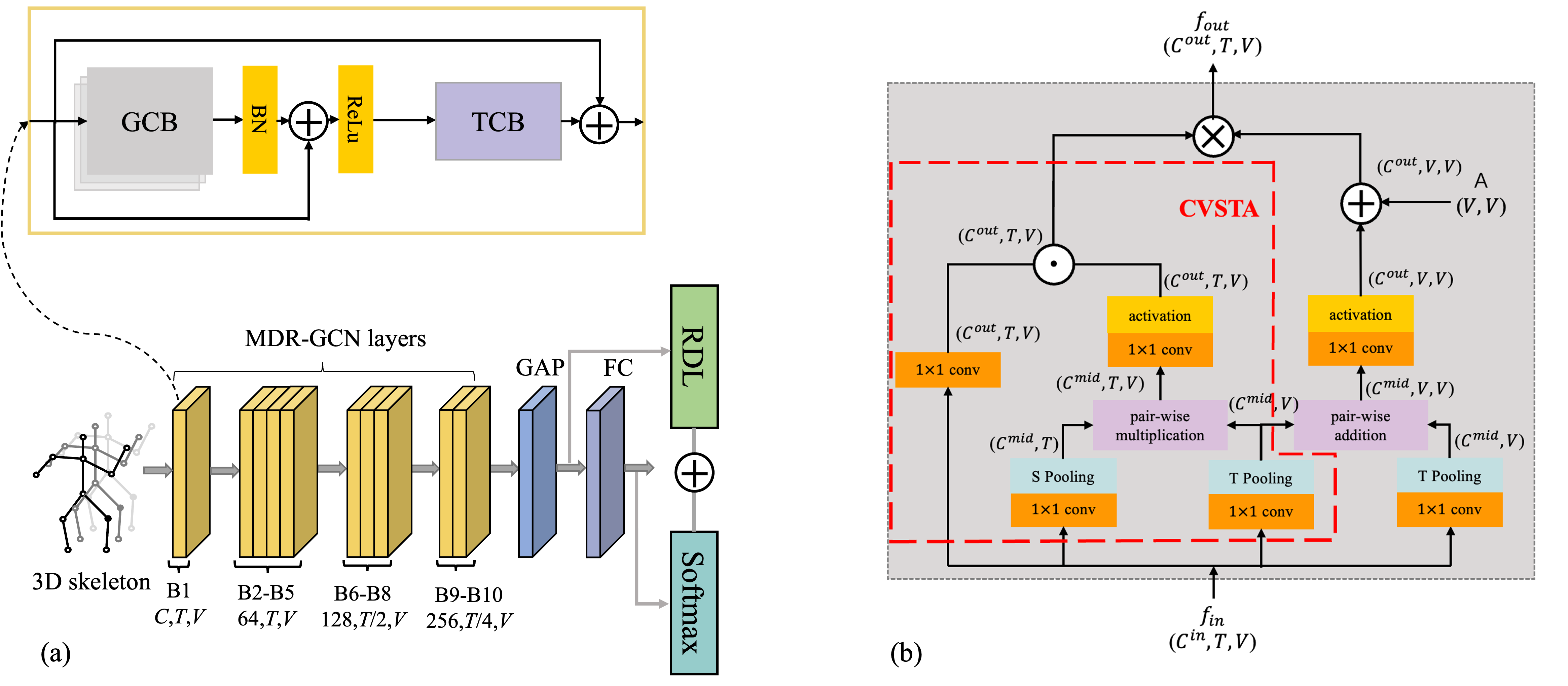
In this section, we first formulate conventional graph convolution. Then, we elaborate Channel-Variable Spatial-Temporal Attention (CVSTA) and Multi-Dimensional Refinement Graph Convolution Network (MDR-GCN). Finally, we introduce Robust Decouple Loss (RDL). The overall architecture of our model is shown in Figure 3.
III-A Preliminaries
The skeletal graph is established according to the natural connections of the human skeleton, where denotes the set of skeletal nodes. Set of edges is formulated as a corresponding adjacency matrix with the element which reflects the degree of relevance between and (). In spatial view, the graph convolution operation on node is expressed as
| (1) |
where denotes the input features of . represents the weight vector of the convolution operation, which transfers the number of input features from to .
III-B Model implementation
The above spatial graph convolution process is not intuitive for task-adapted GCN of action analysis which is introduced as follows. Concretely, a frames input sample with channels is a tensor. Spatial-temporal graph convolution can be defined by transformed Eq.1 as
| (2) |
where is the output feature tensor with channels. denotes the weight matrix to adjust the number of learnable topology subsets , where . Our is initialized the same as ST-GCN [7].
Channel-Variable Spatial-Temporal Attention To avoid limiting the channel power for the fine-grained action recognition task, our CVSTA reinforces attention to extract more discriminative spatial-temporal features of the input . CVSTA consists of three parts: discriminative spatial-temporal saliency representation, feature transformation, and feature modeling. The implementation details are described as follows.
Discriminative Spatial Temporal Saliency Representation. To obtain discriminative representation, we first involve convolution to generate variable channels of current middle layer for distinctive layer and its (This means a different layer and its may set a different ). We claim that the middle layer is necessary for enhancing the discriminative representation, and the value of may always be different from that of . This is because spatial-temporal saliency representation, refinement tensor, and spatial attention should not share the same for their maximum discriminative channel power in a model.
Then, feature compaction is achieved by generating the pooled temporal vector and the spatial one which are calculated by average pooling along with the spatial dimension and the frame direction of . With and , the saliency weights of spatial-temporal joints can be calculated as
| (3) |
where denotes the parameters of the convolution. is the activation function, and indicates pair-wise multiplication.
Feature Transformation. In parallel with saliency representation, feature transformation is implemented by transforming to the output tensor by convolution for computing the following refinement tensor.
Feature Modelling. To achieve CVSTA, we finally adopt pair-wise element-level fusion of and for obtaining spatial-temporal refinement tensor , which is expressed as
| (4) |
where represents the Hadamard product. In CVSTA, the number of input, middle, and output channels entirely relies on the deployed model, therefore, could flexibly deploy on different graph convolutional models.
Graph Convolution Block The method for refining the spatial topology of joints is similar to CVSTA. Like the operation of generating , we use convolution, pooling, and shape transformation operations on to get . We represent the spatial correlations of the motions as the spatial tensor , which is formulated as
| (5) |
where denotes the parameters of convolution. represents the pair-wise addition. Note that we share of CVSTA as a spatial pooled vector which could reduce the cost of computation and offers an additional spatial-temporal relationship for and . Combining CVSTA with spatial attention, our graph convolution operation can be written as
| (6) |
where and indicate and of the subset (), respectively. is a learnable parameter that could balance the value between and shared . Our GCB is achieved by the above channel, spatial-temporal, and spatial refinements.
Multi-Dimensional Refinement Graph Convolution Network A complete MDR-GCN layer comprises a graph convolutional block (GCB), a temporal convolutional block (TCB), and a residual structure. To enhance the learning of the relationships between nearby frames, there are kernels in all temporal convolutions (kernel size , in our work).
In MDR-GCN, there are a total of 10 MDR-GCN layers. The numbers of output channels for each layer are ordered by 64-64-64-64-128-128-128-256-256-256. A global average pooling layer and a softmax classifier combing with RDL embedding loss are performed at the end.
III-C Robust Decouple Loss
To further enhance the discriminative capability of our fine-grained classification network, we propose the Robust Decouple Loss, which combines both numerical-balanced angular and norm-based losses replacing the center loss. Angle losses utilize both intra-class angle loss and inter-class one to optimize margins among classes in the angle view. Along with the norm aspect, is designed for coinciding intra-class-sample norms.
| (7) |
where is the size of a mini-batch, and indicates the final output of the FC layer with features of the sample with the corresponding label for classes, . , which represents the center of the class, is randomly initialized and updated in the training process.
In addition, inter-class angular loss , which is involved in enlarging the margins among different classes, can be written as
| (8) |
Compared with the penalized square form of , is free of the square to equalize the inter-class angular margins in the training process.
For one FC feature , the boundaries of and are (0, 4) and (0, 2), respectively. A large ( in our work) always causes large , and . Thus, is not suitable for numerical balance because of its large value of the initial weights. Fractional formed loss between and is more reasonable in numerical consideration. The intra-class norm-specific loss can be expressed as
| (9) |
| (10) |
where denotes the robust ratio expression. This fraction design eliminates the weak robustness in orders of magnitude between the FC feature and its center. indicates similar norms of the two elements in . A small parameter is utilized to avoid division by zero. Nevertheless, the value of is always large enough to set in most cases.
By combining , and , RDL implements robust class-wise discriminative embedding for strengthening the fine-grained classification. RDL is computed as
| (11) |
Motivated by fine-grained angular loss, RDL is dominated by appending auxiliary and . The hyperparameters and (always setting ) are used to weigh the three losses. Inter-class norm-based loss, which leads to a numerical imbalance issue, is free of design in this paper. Consequently, the fine-grained action classification loss can be achieved by combining softmax loss and embedding loss RDL.
| (12) |
| (13) |
where denotes the column of the weights in the last FC layer and is the bias term. Finally, the loss function can achieve class-wise discriminative learning for fine-grained classification.
III-D Gradients calculation of RDL
In this subsection, we describe the derivation process of RDL. According to Eq.11, the gradients of RDL are the sum of three items, which can be expressed as
| (14) |
For , as and with respect to is symmetrical to , the gradients in the angle items with respect to is the similar to . Therefore, we only need to pay extra attention to the update equation of in . Then, we solve for the gradients of each item.
The gradients of in can be transfered as
| (15) |
Based on Eq.7, can be expressed as
| (16) |
The gradients of with respect to are formulated as
| (17) |
where indicates an identity matrix.
The gradients of According to Eq.8, can be written as
| (18) |
The gradients of with respect to are formulated as
| (19) |
The gradients of
is expressed as
| (20) |
The gradients of concerning are formulated as
| (21) |
And the gradients of with respect to are represented as
| (22) |
IV Experiments
IV-A Datasets
FineGym99 FineGym99 [52] is a fine-grained action recognition dataset containing 29k videos of 99 fine-grained gymnastics action categories. Compared to existing action recognition datasets, it provides temporal annotations at both action and sub-action levels with a three-level semantic hierarchy. We conduct experiments using 3D-pose extracted the same as Pyskl [53]. The dataset is publicly available at https://sdolivia.github.io/FineGym/.
FSD-10 To fully evaluate the effectiveness of spatial-temporal modules in our network, FSD-10 [54] is involved in our experiments. FSD-10 collects 1484 clips from the worldwide figure skating championships in 2017–2018 and contains ten fine-grained actions in men/ladies’ programs. Each clip is at 30 fps with a resolution of . There are 1500 frames for each sample and 25 joints for each frame. This dataset has a significant duration variance. Therefore we can better verify the performance of our method in the temporal view. The dataset is publicly available at https://shenglanliu.github.io/fsd10/. I NTU RGB+D NTU RGB+D [55] is a large-scale human action recognition dataset that contains 56800 clips of actions. The action samples are categorized into 60 classes, where 50 classes have single-person actions, and the rest are pair interactive actions. We adopt 25 joints to represent each frame of one person (no more than two persons). We recommend two split versions for conducting experiments, i.e., cross-subject and cross-view. In cross-subject, the dataset is of 40320 training samples and 16560 testing samples. The training set of X-view obtains 37920 samples via the and cameras. The camera generates the corresponding testing set, which consists of 18960 samples. We utilize both two versions for experiments in this paper. The dataset is publicly available at https://rose1.ntu.edu.sg/dataset/actionRecognition/.
| Models | CVSTA | RDL | Accuracy(%) |
|---|---|---|---|
| ST-GCN | 86.59 | ||
| ✓ | 88.71 | ||
| ✓ | 87.29 | ||
| ✓ | ✓ | 89.65 | |
| CTR-GCN | 90.59 | ||
| ✓ | 90.82 | ||
| ✓ | 92.00 | ||
| ✓ | ✓ | 92.94 |
| Settings | Accuracy(%) | |
|---|---|---|
| Cf | 90.59 | |
| C16 | 92.71 | |
| C8 | 93.88 | |
| C4 | 93.88 |
| Settings | Attentions | Models | Accuracy(%) |
|---|---|---|---|
| A | SA-GC | InfoGCN [13] | 91.9 |
| B | ST-JointAtt | Efficient-GCN b4 [15] | 92.6 |
| C | CVTSA | MDR-GCN | 93.3 |
| Methods | 0% noise (%) | 1% noise (%) | 10% noise (%) |
|---|---|---|---|
| CTR-GCN | 90.58 | 89.65 | 85.88 |
| MDR-GCN (wo RDL) | 91.06 | 90.82 | 87.13 |
| MDR-GCN | 93.18 | 92.47 | 91.29 |
| Accuracy(%) | |||
| 91.06 | |||
| ✓ | 91.76 | ||
| ✓ | 91.29 | ||
| ✓ | 90.35 | ||
| ✓ | ✓ | 92.00 | |
| ✓ | ✓ | 92.94 | |
| ✓ | ✓ | 92.25 | |
| ✓ | ✓ | ✓ | 93.18 |
| Settings | Accuracy(%) | ||
|---|---|---|---|
| H1 | hardswish | 1 | 90.35 |
| T1 | tanh | 1 | 90.82 |
| S1 | sigmoid | 1 | 90.82 |
| S2 | sigmoid | 2 | 90.82 |
| T2 | tanh | 2 | 91.06 |
| T3 | tanh | 3 | 90.59 |
| Models | Params | FLOPs | Accuracy(%) |
|---|---|---|---|
| MS-G3D | 2.8M | 24.7G | 92.0 |
| CTR-GCN | 1.2M | 14.4G | 91.9 |
| PoseC3D | 2.0M | 15.9G | 93.2 |
| MDR-GCN | 1.3M | 15.3G | 93.3 |
| Methods | FSD-10(%) | FineGym99(%) |
| Baseline | 91.06 | 90.13 |
| center loss [19] | 91.06 | 91.17 |
| sphereFace [22] | 88.24 | – |
| LMCL[49] | 92.24 | – |
| arcFace [24] | 92.71 | 91.52 |
| LACE [27] | 91.29 | 91.74 |
| RDL without | 92.94 | 91.94 |
| RDL | 93.18 | 92.11 |
| Methods | Accuracy(%) |
|---|---|
| ST-GCN [7] | 36.4 |
| MS-G3D [56] | 92.0 |
| CTR-GCN [11] | 91.9 |
| MS-G3D++ [41] | 92.6 |
| InfoGCN [13] | 92.0 |
| PoseC3D [41] | 94.3 |
| MDR-GCN | 94.5 |
| Methods | Accuracy(%) |
|---|---|
| ST-GCN [7] | 84.24 |
| 2S-AGCN [8] | 88.23 |
| AS-GCN [57] | 86.82 |
| MS-G3D [56] | 88.72 |
| CTR-GCN [11] | 90.58 |
| InfoGCN [13] | 91.76 |
| MDR-GCN | 94.18 |
| Methods | X-sub(%) | X-view(%) |
|---|---|---|
| ST-GCN [7] | 81.5 | 88.3 |
| 2S-AGCN [8] | 88.5 | 95.1 |
| AS-GCN [57] | 86.8 | 94.2 |
| Shift-GCN [38] | 90.7 | 96.5 |
| DC-GCN+ADG [58] | 90.8 | 96.6 |
| Dynamic GCN [37] | 91.5 | 96.0 |
| MSIN [58] | 91.5 | 96.5 |
| MS-G3D [56] | 91.5 | 96.2 |
| MSG3D++ [41] | 92.2 | 96.6 |
| MST-GCN [59] | 91.5 | 96.6 |
| CTR-GCN [11] | 92.4 | 96.8 |
| Efficient-GCN B4 [15] | 92.1 | 96.1 |
| InfoGCN [13] | 93.0 | 97.1 |
| PoseC3D [41] | 94.1 | 97.1 |
| MDR-GCN | 92.8 | 97.2 |
IV-B Training details
We conducted all experiments on the PyTorch deep learning framework. Stochastic gradient descent (SGD) with Nesterov momentum (0.9) is applied as the optimization strategy, and the learning rate is set to 0.1. For FineGym99, we set the batch size to 64, and the learning rate is divided by ten at 60 and 120 epochs. For FSD-10, the learning rate multiply by 0.1 at epochs 150 and 225 for 300 epochs, 256 non-zero frames, and 48 batch size is set in Sec 4.3, Sec 4.4, all frames and 8 batch size are utilized to show the complete performance in Sec 4.5, Sec 4.6. For NTU RGB+D, the batch size is set to 64, and the learning rate decays with a factor of 0.1 at epochs 35 and 55 for a total of 65 epochs.
IV-C Ablation study
Expandability of our method To evaluate the effectiveness of the CVSTA block, we plugged it into ST-GCN [7] and CTR-GCN [11]. As can be seen in Table I, the experimental results of plugged ST-GCN and CTR-GCN can improve performance than their corresponding original versions on the FSD-10 dataset. Compared with the original ST-GCN, CVSTA plus ST-GCN can reach an enormous improvement of . CTR-GCN can also be enhanced performance () by combining with CVSTA. The above experimental results demonstrate that CVSTA is effective for fine-grained action recognition, especially for the attention-free method (e.g., ST-GCN). For evaluating the effectiveness of the proposed discriminative loss, RDL is attached to ST-GCN, CTR-GCN, and CTR-GCN+CVSTA. As shown in Table I, the three RDL-attached methods exceed corresponding ST-GCN, CTR-GCN, and CTR-GCN+CVSTA by , and , respectively. According to the above experimental results, CVSTA and RDL plugged methods can outperform the baseline models. This illustrates that CVSTA can increase spatial-temporal discrimination. Besides, RDL can achieve more excellent performance by combining the discrimination-reinforced networks. Thus, CVSTA is beneficial for reinforcing the power of RDL for our fine-grained task.
Effectiveness of the variable channel We utilize different in CVSTA with RDL to examine the effect of changing channels. As shown in Table II, (1) compared to the fixed setting (setting Cf), any configuration which utilizes a variable channel outperforms the fixed setting, indicating the variable channels enhance the capability of perceiving the latent and filtering out the redundant features. (2) comparing settings C16 and C8, we find that compression of the channel results in abandoning valid information. Therefore, we choose C8 collocation as our configuration, considering both performance and space consumption.
Effectiveness of our spatial-temporal attention To ascertain that CVSTA is providing more high-quality features, we train our framework by using different attention on the FineGym99 dataset. As Table III shows, settings B and C show higher performance compare to the non-spatial-temporal SA-GC attention block (setting A). And comparing settings B and C, we see that CVSTA consistently outperforms the spatial-temporal attention which being utilized after GCN and TCN layers.
Effectiveness of our method for noisy data To have a deeper understanding of the robustness of our model, we modify the FSD-10 dataset by setting the random coordinates in some (1%, 10%) skeletal data to 0. Table IV shows the performance of our method on the modified-FSD-10 dataset. Based on the comparison between 1% and 10%, we can see when there are more outliers on a dataset, our method can reflect obvious performance advantages.
Effectiveness of RDL We set the performance of MDR-GCN without RDL () as the baseline to investigate the effectiveness of RDL terms via setting , . Table V illustrates angular terms of RDL can enhance the performance by comparing with the baseline. In contrast, norm-specific RDL without angular terms would reduce the performance (). This illustrates angular terms are more important than the norm-based one for the fine-grained action recognition task. Besides, the norm-based term is helpful for the angular terms of RDL (). The results and analyses coincide with our design of RDL.
Configuration of MDR-GCN Table VI shows the effects of activation function and the number of TCN blocks in different settings. As shown in Table VI, various settings achieve similar results, illustrating our model’s robustness. The details are as follows. According to the experimental results of H1, T1, and S1 collocations, both tanh and sigmoid activation functions are acceptable options. By adjusting , the different results of both S2 and T2 indicate that the tanh activation function is superior to others. Besides, the results of variable in T1, T2, and T3 encourage us to choose multi-kernel (i.e., ) for MDR-GCN. However, a large may reduce the performance because of over-learning and enlarging the network’s parameters. Considering both performance and efficiency, we choose T2 collocation as our configuration.
Efficiency of our method In performance comparison between our method and C3D, we adopt the input shape for PoseC3D, for MS-G3D, CTR-GCN and our method. Table VII shows that under such configuration, our method achieves more competitive performance and efficiency on the FineGym99 dataset.
IV-D Comparison with other loss functions
Table VIII shows the performances of advanced loss functions on FSD-10 and FineGym99. For a fair comparison, we use the C8 configuration of Table II in the rest experiments of this paper. We observe that (1) on FSD-10, RDL gains a improvement over the center loss, which indicates the effectiveness of the proposed embedding loss. Besides, our loss version (RDL without ) and center loss contain two similar optimization properties (i.e., angle and norm). In this case, also outperforms center loss by , which illustrates the robustness of our loss design. (2) RDL achieves an accuracy of , which surpasses the state-of-the-art implicit losses in recent years, including competitive arcFace loss (). To further illustrate the effectiveness of RDL, we involve the competitive arcFace and recent LACE for comparison on the FineGym99 dataset. RDL outperforms arcFace and LACE by and , respectively. The results of FineGym99 indicate that RDL is adequate and robust for fine-grained datasets with large-scale classes.
IV-E Visualization of CVSTA
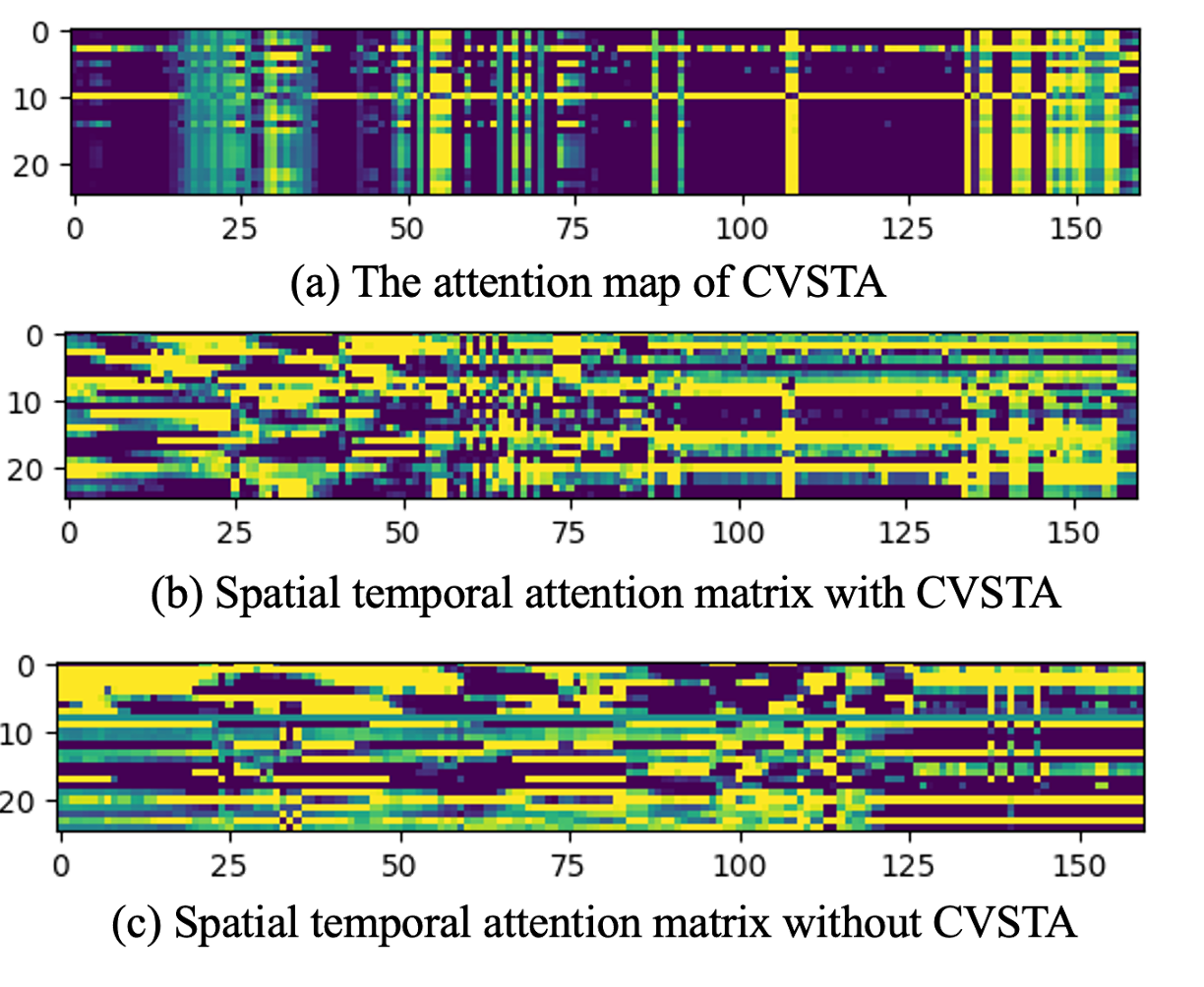
We obtain the experimental sample by trimming ’3StepSequence3’ of FSD-10 to visualize the attention map of CVSTA (Figure 4 (a)). Frame extraction strategy is excluded to ensure the frame coincides with the pose temporal position of the original action. We reveal the first 160 frames as the sample in the untrimmed joint sequence, which includes most of the continuous key poses. We further illustrate that the first 120 frames of the sample express a sliding sequence part, and the rest represent a complex technical sequence. The joint (right knee) should be highlighted in most frames because of the intuitive plain sequence. As shown in Figure 4, visualization of the attention map provides a clear focus in the joint row. The visualization results illustrate that CVSTA is effective for spatial joints.
Furthermore, a few body twists are performed in the temporal neighborhood of the frame, leading to highlighted shoulder joints by CVSTA during this period. Thus, we can confirm that CVSTA achieves spatial-temporal attention. Compared with the sliding sequence part, most of the frames of the technical sequence part are highlighted in the attention map. This shows that our CVSTA provides additional attention to the temporal dimension. As shown in Figure 4 (b) and (c), the visualization of with CVSTA also shows more excellent results in the above position than those without CVSTA. This indicates CVSTA is a benefit for extracting key frames to cope with large duration variance action samples.
IV-F Visualization of RDL
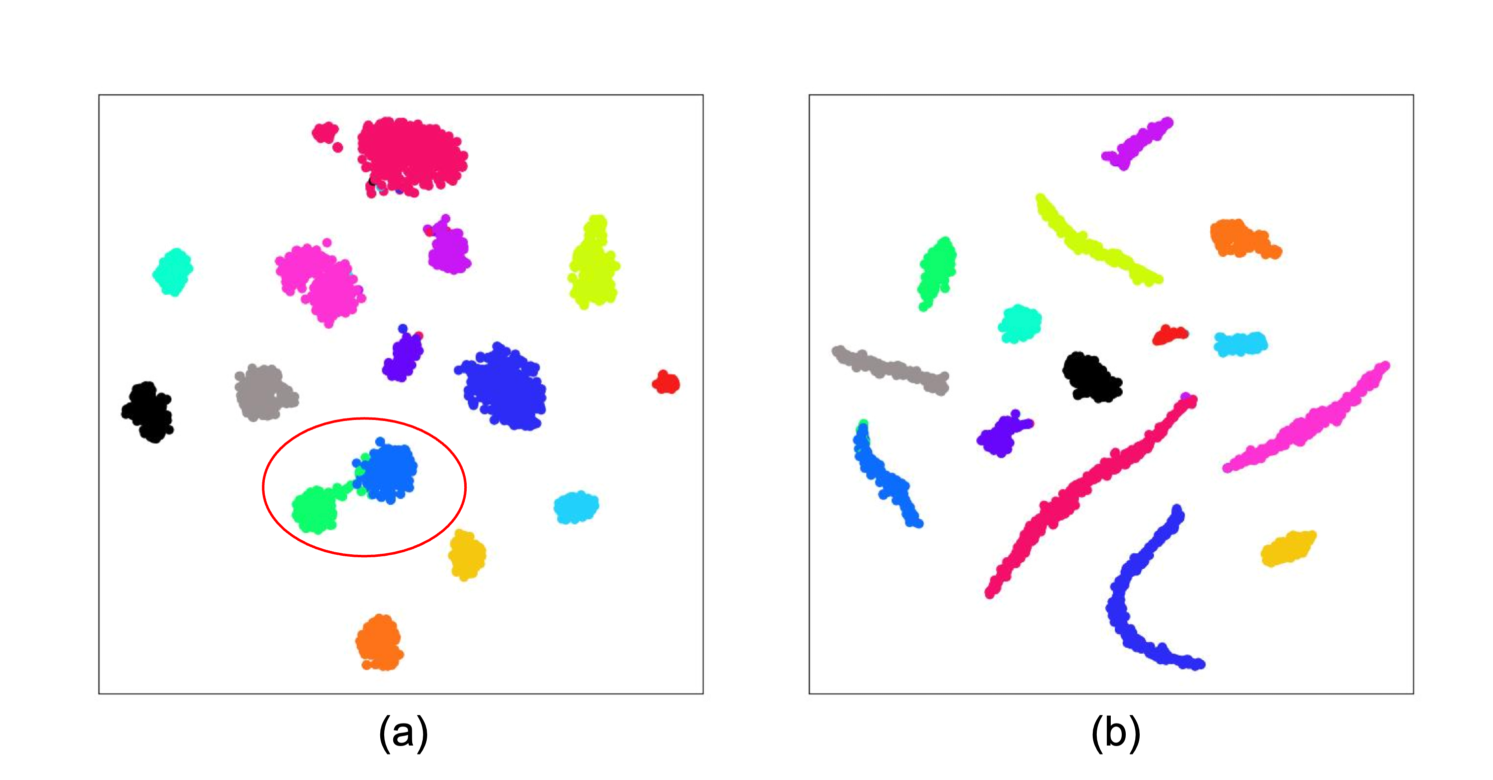
We use the MDR-GCN model on the FineGym99 dataset, which employs (a) Softmax loss and (b) RDL as loss functions, and perform t-SNE [60] dimensionality reduction on the generated features for 15 classes with more samples. Figure 5 shows the results after dimensionality reduction. We observe that (1) there are significantly more outliers in (a) than in (b), which reflects the good robustness of RDL. (2) For some hard-to-distinguish classes (such as the two classes inside the red circle in (a)), RDL can better achieve class separability.
IV-G Comparison with the State-of-the-Art
In this subsection, we compare our method with the state-of-the-art skeleton-based action recognition methods on all three datasets introduced above. FineGym99 and FSD-10 are utilized in fine-grained tasks to evaluate our approach’s advantages on spatial-temporal joints and large-scale classes. To show the generality of our model, the most widely used dataset NTU RGB+D is employed for comparison. On NTU RGB+D and FineGym99 dataset, our performance is fused by the results of multiple skeletal modalities as the mainstream methods [11, 41, 13].
The results are shown in Tables IX, X and XI. Our model achieves state-of-the-art performance with a large margin on the Fine-Grained datasets. And on NTU RGB+D, our method also gets close to the state-of-the-art models considering both evaluation benchmarks. This illustrates that, as a fine-grained solution, our method can still preserve good capability on coarse-grained datasets.
V Limitations and Social Impacts
Currently, we only explore the performance of RDL on skeleton-based action recognition, but RDL may also be applied in other fine-grained tasks, which need to be explored in future work. Furthermore, although RDL improves the robustness problem by decoupling the Euclidean distance as an explicit method, the effect of outliers on the center still exists.
Our method achieves a significant improvement in the accuracies of fine-grained action recognition, which could provide a new solution for recognizing complex and similar actions (such as technical actions in gymnastics, diving, figure skating, etc.) that are common in reality. There are no known socially detrimental effects of our work other than those typically associated with developing new AI systems.
VI Conclusion
This work proposes a Multi-Dimensional Refinement Graph Convolution Network for fine-grained skeleton-based action recognition (MDR-GCN), including a Channel-Variable Spatial-Temporal Attention (CVSTA). The model is powerful for extracting spatial and temporal discriminative features. Furthermore, we propose a Robust Decouple Loss, which can enhance intra-class compactness and inter-class separability for the fine-grained recognition task. Our method outperforms the existing skeleton-based approaches on the three challenging datasets. Meanwhile, the flexibility of RDL and CVSTA could improve future work.
References
- [1] C. Zhong, L. Hu, Z. Zhang, Y. Ye, and S. Xia, “Spatio-temporal gating-adjacency gcn for human motion prediction,” in Proceedings of the IEEE/CVF Conference on Computer Vision and Pattern Recognition, 2022, pp. 6447–6456.
- [2] Y. Du, W. Wang, and L. Wang, “Hierarchical recurrent neural network for skeleton based action recognition,” in Proceedings of the IEEE conference on computer vision and pattern recognition, 2015, pp. 1110–1118.
- [3] J. Liu, A. Shahroudy, D. Xu, and G. Wang, “Spatio-temporal lstm with trust gates for 3d human action recognition,” in European conference on computer vision. Springer, 2016, pp. 816–833.
- [4] S. Song, C. Lan, J. Xing, W. Zeng, and J. Liu, “An end-to-end spatio-temporal attention model for human action recognition from skeleton data,” in Proceedings of the AAAI conference on artificial intelligence, vol. 31, no. 1, 2017.
- [5] H. Liu, J. Tu, and M. Liu, “Two-stream 3d convolutional neural network for skeleton-based action recognition,” arXiv preprint arXiv:1705.08106, 2017.
- [6] Y. Hou, Z. Li, P. Wang, and W. Li, “Skeleton optical spectra-based action recognition using convolutional neural networks,” IEEE Transactions on Circuits and Systems for Video Technology, vol. 28, no. 3, pp. 807–811, 2016.
- [7] S. Yan, Y. Xiong, and D. Lin, “Spatial temporal graph convolutional networks for skeleton-based action recognition,” in Thirty-second AAAI conference on artificial intelligence, 2018.
- [8] L. Shi, Y. Zhang, J. Cheng, and H. Lu, “Two-stream adaptive graph convolutional networks for skeleton-based action recognition,” in Proceedings of the IEEE/CVF conference on computer vision and pattern recognition, 2019, pp. 12 026–12 035.
- [9] Y.-F. Song, Z. Zhang, C. Shan, and L. Wang, “Richly activated graph convolutional network for robust skeleton-based action recognition,” IEEE Transactions on Circuits and Systems for Video Technology, vol. 31, no. 5, pp. 1915–1925, 2020.
- [10] J. Gao, T. He, X. Zhou, and S. Ge, “Skeleton-based action recognition with focusing-diffusion graph convolutional networks,” IEEE Signal Processing Letters, vol. 28, pp. 2058–2062, 2021.
- [11] Y. Chen, Z. Zhang, C. Yuan, B. Li, Y. Deng, and W. Hu, “Channel-wise topology refinement graph convolution for skeleton-based action recognition,” in Proceedings of the IEEE/CVF International Conference on Computer Vision, 2021, pp. 13 359–13 368.
- [12] X. Shu, J. Yang, R. Yan, and Y. Song, “Expansion-squeeze-excitation fusion network for elderly activity recognition,” IEEE Transactions on Circuits and Systems for Video Technology, vol. 32, no. 8, pp. 5281–5292, 2022.
- [13] H.-g. Chi, M. H. Ha, S. Chi, S. W. Lee, Q. Huang, and K. Ramani, “Infogcn: Representation learning for human skeleton-based action recognition,” in Proceedings of the IEEE/CVF Conference on Computer Vision and Pattern Recognition, 2022, pp. 20 186–20 196.
- [14] D. Ahn, S. Kim, H. Hong, and B. C. Ko, “Star-transformer: A spatio-temporal cross attention transformer for human action recognition,” in Proceedings of the IEEE/CVF Winter Conference on Applications of Computer Vision, 2023, pp. 3330–3339.
- [15] Y.-F. Song, Z. Zhang, C. Shan, and L. Wang, “Constructing stronger and faster baselines for skeleton-based action recognition,” IEEE Transactions on Pattern Analysis and Machine Intelligence, 2022.
- [16] D. Chang, Y. Ding, J. Xie, A. K. Bhunia, X. Li, Z. Ma, M. Wu, J. Guo, and Y.-Z. Song, “The devil is in the channels: Mutual-channel loss for fine-grained image classification,” IEEE Transactions on Image Processing, vol. 29, pp. 4683–4695, 2020.
- [17] S. Li, T. Liu, J. Tan, D. Zeng, and S. Ge, “Trustable co-label learning from multiple noisy annotators,” IEEE Transactions on Multimedia, 2021.
- [18] S. Li, X. Xia, S. Ge, and T. Liu, “Selective-supervised contrastive learning with noisy labels,” in Proceedings of the IEEE/CVF Conference on Computer Vision and Pattern Recognition, 2022, pp. 316–325.
- [19] Y. Wen, K. Zhang, Z. Li, and Y. Qiao, “A discriminative feature learning approach for deep face recognition,” in European conference on computer vision. Springer, 2016, pp. 499–515.
- [20] X. He, Y. Zhou, Z. Zhou, S. Bai, and X. Bai, “Triplet-center loss for multi-view 3d object retrieval,” in Proceedings of the IEEE conference on computer vision and pattern recognition, 2018, pp. 1945–1954.
- [21] W. Liu, Y. Wen, Z. Yu, and M. Yang, “Large-margin softmax loss for convolutional neural networks,” arXiv preprint arXiv:1612.02295, 2016.
- [22] W. Liu, Y. Wen, Z. Yu, M. Li, B. Raj, and L. Song, “Sphereface: Deep hypersphere embedding for face recognition,” in Proceedings of the IEEE conference on computer vision and pattern recognition, 2017, pp. 212–220.
- [23] F. Wang, J. Cheng, W. Liu, and H. Liu, “Additive margin softmax for face verification,” IEEE Signal Processing Letters, vol. 25, no. 7, pp. 926–930, 2018.
- [24] J. Deng, J. Guo, N. Xue, and S. Zafeiriou, “Arcface: Additive angular margin loss for deep face recognition,” in Proceedings of the IEEE/CVF conference on computer vision and pattern recognition, 2019, pp. 4690–4699.
- [25] M. Kim, A. K. Jain, and X. Liu, “Adaface: Quality adaptive margin for face recognition,” in Proceedings of the IEEE/CVF Conference on Computer Vision and Pattern Recognition, 2022, pp. 18 750–18 759.
- [26] Y. Zhang, Y. Huang, S. Yu, and L. Wang, “Cross-view gait recognition by discriminative feature learning,” IEEE Transactions on Image Processing, vol. 29, pp. 1001–1015, 2019.
- [27] J. Peeples, C. H. McCurley, S. Walker, D. Stewart, and A. Zare, “Learnable adaptive cosine estimator (lace) for image classification,” in Proceedings of the IEEE/CVF Winter Conference on Applications of Computer Vision, 2022, pp. 3479–3489.
- [28] L. Li, W. Zheng, Z. Zhang, Y. Huang, and L. Wang, “Skeleton-based relational modeling for action recognition. corr abs/1805.02556 (2018),” 1805.
- [29] X. Jiang, K. Xu, and T. Sun, “Action recognition scheme based on skeleton representation with ds-lstm network,” IEEE Transactions on Circuits and Systems for Video Technology, vol. 30, no. 7, pp. 2129–2140, 2019.
- [30] M. Henaff, J. Bruna, and Y. LeCun, “Deep convolutional networks on graph-structured data,” arXiv preprint arXiv:1506.05163, 2015.
- [31] T. Soo Kim and A. Reiter, “Interpretable 3d human action analysis with temporal convolutional networks,” in Proceedings of the IEEE conference on computer vision and pattern recognition workshops, 2017, pp. 20–28.
- [32] C. Li, Q. Zhong, D. Xie, and S. Pu, “Skeleton-based action recognition with convolutional neural networks,” in 2017 IEEE International Conference on Multimedia & Expo Workshops (ICMEW). IEEE, 2017, pp. 597–600.
- [33] C. Cao, C. Lan, Y. Zhang, W. Zeng, H. Lu, and Y. Zhang, “Skeleton-based action recognition with gated convolutional neural networks,” IEEE Transactions on Circuits and Systems for Video Technology, vol. 29, no. 11, pp. 3247–3257, 2018.
- [34] C. Li, C. Xie, B. Zhang, J. Han, X. Zhen, and J. Chen, “Memory attention networks for skeleton-based action recognition,” IEEE Transactions on Neural Networks and Learning Systems, vol. 33, no. 9, pp. 4800–4814, 2021.
- [35] D. I. Shuman, S. K. Narang, P. Frossard, A. Ortega, and P. Vandergheynst, “The emerging field of signal processing on graphs: Extending high-dimensional data analysis to networks and other irregular domains,” IEEE signal processing magazine, vol. 30, no. 3, pp. 83–98, 2013.
- [36] T. Kipf, E. Fetaya, K.-C. Wang, M. Welling, and R. Zemel, “Neural relational inference for interacting systems,” in International Conference on Machine Learning. PMLR, 2018, pp. 2688–2697.
- [37] F. Ye, S. Pu, Q. Zhong, C. Li, D. Xie, and H. Tang, “Dynamic gcn: Context-enriched topology learning for skeleton-based action recognition,” in Proceedings of the 28th ACM International Conference on Multimedia, 2020, pp. 55–63.
- [38] K. Cheng, Y. Zhang, X. He, W. Chen, J. Cheng, and H. Lu, “Skeleton-based action recognition with shift graph convolutional network,” in Proceedings of the IEEE/CVF Conference on Computer Vision and Pattern Recognition, 2020, pp. 183–192.
- [39] Z. Qin, Y. Liu, P. Ji, D. Kim, L. Wang, R. McKay, S. Anwar, and T. Gedeon, “Fusing higher-order features in graph neural networks for skeleton-based action recognition,” IEEE Transactions on Neural Networks and Learning Systems, 2022.
- [40] K. Cheng, Y. Zhang, C. Cao, L. Shi, J. Cheng, and H. Lu, “Decoupling gcn with dropgraph module for skeleton-based action recognition,” in European Conference on Computer Vision. Springer, 2020, pp. 536–553.
- [41] H. Duan, Y. Zhao, K. Chen, D. Lin, and B. Dai, “Revisiting skeleton-based action recognition,” in Proceedings of the IEEE/CVF Conference on Computer Vision and Pattern Recognition, 2022, pp. 2969–2978.
- [42] I. Masi, Y. Wu, T. Hassner, and P. Natarajan, “Deep face recognition: A survey,” in 2018 31st SIBGRAPI conference on graphics, patterns and images (SIBGRAPI). IEEE, 2018, pp. 471–478.
- [43] M. Wang and W. Deng, “Deep face recognition: A survey,” Neurocomputing, vol. 429, pp. 215–244, 2021.
- [44] R. Hadsell, S. Chopra, and Y. LeCun, “Dimensionality reduction by learning an invariant mapping,” in 2006 IEEE Computer Society Conference on Computer Vision and Pattern Recognition (CVPR’06), vol. 2. IEEE, 2006, pp. 1735–1742.
- [45] K. Sohn, “Improved deep metric learning with multi-class n-pair loss objective,” Advances in neural information processing systems, vol. 29, 2016.
- [46] A. Hermans, L. Beyer, and B. Leibe, “In defense of the triplet loss for person re-identification,” arXiv preprint arXiv:1703.07737, 2017.
- [47] J. Wang, F. Zhou, S. Wen, X. Liu, and Y. Lin, “Deep metric learning with angular loss,” in Proceedings of the IEEE international conference on computer vision, 2017, pp. 2593–2601.
- [48] F. Wang, X. Xiang, J. Cheng, and A. L. Yuille, “Normface: L2 hypersphere embedding for face verification,” in Proceedings of the 25th ACM international conference on Multimedia, 2017, pp. 1041–1049.
- [49] H. Wang, Y. Wang, Z. Zhou, X. Ji, D. Gong, J. Zhou, Z. Li, and W. Liu, “Cosface: Large margin cosine loss for deep face recognition,” in Proceedings of the IEEE conference on computer vision and pattern recognition, 2018, pp. 5265–5274.
- [50] X. Zhang, R. Zhao, Y. Qiao, X. Wang, and H. Li, “Adacos: Adaptively scaling cosine logits for effectively learning deep face representations,” in Proceedings of the IEEE/CVF Conference on Computer Vision and Pattern Recognition, 2019, pp. 10 823–10 832.
- [51] B. Liu, W. Deng, Y. Zhong, M. Wang, J. Hu, X. Tao, and Y. Huang, “Fair loss: Margin-aware reinforcement learning for deep face recognition,” in Proceedings of the IEEE/CVF International Conference on Computer Vision, 2019, pp. 10 052–10 061.
- [52] D. Shao, Y. Zhao, B. Dai, and D. Lin, “Finegym: A hierarchical video dataset for fine-grained action understanding,” in Proceedings of the IEEE/CVF conference on computer vision and pattern recognition, 2020, pp. 2616–2625.
- [53] H. Duan, J. Wang, K. Chen, and D. Lin, “Pyskl: Towards good practices for skeleton action recognition,” arXiv preprint arXiv:2205.09443, 2022.
- [54] S. Liu, X. Liu, G. Huang, H. Qiao, L. Hu, D. Jiang, A. Zhang, Y. Liu, and G. Guo, “Fsd-10: A fine-grained classification dataset for figure skating,” Neurocomputing, vol. 413, pp. 360–367, 2020.
- [55] A. Shahroudy, J. Liu, T.-T. Ng, and G. Wang, “Ntu rgb+ d: A large scale dataset for 3d human activity analysis,” in Proceedings of the IEEE conference on computer vision and pattern recognition, 2016, pp. 1010–1019.
- [56] Z. Liu, H. Zhang, Z. Chen, Z. Wang, and W. Ouyang, “Disentangling and unifying graph convolutions for skeleton-based action recognition,” in Proceedings of the IEEE/CVF conference on computer vision and pattern recognition, 2020, pp. 143–152.
- [57] M. Li, S. Chen, X. Chen, Y. Zhang, Y. Wang, and Q. Tian, “Actional-structural graph convolutional networks for skeleton-based action recognition,” in Proceedings of the IEEE/CVF conference on computer vision and pattern recognition, 2019, pp. 3595–3603.
- [58] K. Cheng, Y. Zhang, C. Cao, L. Shi, J. Cheng, and H. Lu, “Decoupling gcn with dropgraph module for skeleton-based action recognition,” in European Conference on Computer Vision. Springer, 2020, pp. 536–553.
- [59] Z. Chen, S. Li, B. Yang, Q. Li, and H. Liu, “Multi-scale spatial temporal graph convolutional network for skeleton-based action recognition,” in Proceedings of the AAAI Conference on Artificial Intelligence, vol. 35, no. 2, 2021, pp. 1113–1122.
- [60] L. Van der Maaten and G. Hinton, “Visualizing data using t-sne.” Journal of machine learning research, vol. 9, no. 11, 2008.