Quantum Synchronization in Presence of Shot Noise

Abstract

Synchronization is a widespread phenomenon encountered in many natural and engineered systems with nonlinear classical dynamics. How synchronization concepts and mechanisms transfer to the quantum realm and whether features are universal or platform specific are timely questions of fundamental interest. Here, we present a new approach to model incoherently driven dissipative quantum systems susceptible to synchronization within the framework of Josephson photonics devices, where a dc-biased Josephson junction creates (non-classical) light in a microwave cavity. The combined quantum compound constitutes a self-sustained oscillator with a neutrally stable phase. Linking current noise to the full counting statistics of photon emission allows us to capture phase diffusion, but moreover permits phase locking to an ac-signal and mutual synchronization of two such devices. Thereby one can observe phase stabilization leading to a sharp emission spectrum as well as unique photon emission statistics revealing shot noise induced phase slips. Two-time perturbation theory is used to obtain a reduced description of the oscillators phase dynamics in form of a Fokker-Planck equation in generalization of classical synchronization theories.

Introduction.— Spontaneous emission is the main way in which light is created in nature. As a basic principle, the moment at which a photon will be emitted is fundamentally indeterminate. Hence, photon creation is described in terms of probabilities and statistics rather than definite predictions. This uncertainty gives rise to an intrinsic shot noise in the granular flow of photons, which may act back on the photon generation process itself. To permit the shot noise to imprint its traits in the emission, the light source must be susceptible to such perturbations. Josephson photonics devices, where Cooper pairs tunneling across a dc-biased Josephson junction create photons in a microwave cavity, are ideally suited to study the quantum nature of microwave generation [1]. The nonlinearity of the Josephson junction is employed to create entangled light [2], photon multiplets [3], or single-photons [4, 5]. These quantum light sources may thus become an important component for quantum technological applications [6, 7] in quantum communication, quantum information processing, and for sensing and imaging tasks, such as envisioned quantum radars [8]. Drawing its energy input from a ‘battery’ instead of a periodic drive leaves the device with the necessary degree of freedom to feel the shot noise of its own microwave emission. This neutrally stable phase, however, is the hallmark characteristic of a self-sustained oscillator, that can synchronize its frequency and phase to a weak external signal [9, 10, 11, 12, 13]. Indeed, the constraining effect of that signal has to compete with shot-noise induced diffusion in this novel platform for quantum synchronization.

Synchronization in the quantum regime has attracted interest recently, both for systems whose classical counterparts show synchronization behavior with the paradigmatic example of the van der Pol oscillator [14, 15, 16, 17, 18, 19, 20, 21], as well as for systems [22, 23, 24, 25, 26, 27, 28, 29], such as small spins, or mechanisms [30, 31, 32, 33] without classical analogue. While synchronization in (multi-mode) Josephson-photonics has been observed in a semiclassical regime [34, 35, 36] and to some extent theoretically described [37, 38, 39], such devices are also particularly suited to study the deep quantum regimes of strong nonlinearity at the few-photon level [5, 3, 40], where such fundamental questions as quantum measures of synchronization [41, 42] and synchronization of individual trajectories [30] can be studied.

Here, we present a model for the quantum dynamics of Josephson-photonics circuit yielding self-sustained oscillations and describe how it synchronizes to an external ac-signal or a second circuit. Phase locking enables an immediate exploitation of such devices as sources of entanglement, thus dispensing with the elaborate scheme developed in [2] to characterize the entanglement of a two-mode squeezed state without phase stability, and opens the door to Wigner state tomography consequently broadening the potential technological impact of these devices. Moreover, the new platform allows studying fundamental limitations of synchronization in the quantum regime by harnessing the linkage between photonic and charge dynamics in our devices [43] to describe quantum shot noise and the phase slips it induces.

Quantum synchronization to an external signal.— In a Josephson-photonics device Cooper pairs tunneling across a dc-biased Josephson junction create photonic excitations in a microwave cavity connected in series with the junction, see Fig. 1(b). The energy of Cooper pairs is converted into microwave radiation emitted from the cavity with a frequency, $\omega_{J}\approx 2eV_{\text{dc}}/\hbar$, when the dc-voltage is tuned close to a resonance frequency, $\omega_{0}\approx\omega_{J}$, of the cavity. Placing a resistor in series with junction and cavity promotes a back-action of the emission on the voltage driving the tunneling process: the mean photon current (which equals the mean dc-current) reduces the effective dc-voltage at the junction, while fluctuations (photonic- and equivalently [43] current-shot–noise) are turned into voltage variations assumed to exceed thermal or other fluctuations of the voltage source. As we demonstrate here, the very same backaction mechanism can help to avert broadening, if a small ac-locking signal is added to the dc-voltage, $V(t)=V_{\text{dc}}+V_{\text{ac}}\cos[\Omega t+\varphi_{\text{ac}}]$. Increasing the amplitude $\varepsilon=2eV_{\text{ac}}/(\hbar\Omega)$, the spectrum will first show an additional small $\delta$-peak at $\Omega$, while the broadened peak is pulled towards $\Omega$, until eventually most light is emitted within a very sharp peak in synch with the external locking drive, see Fig. 1(c). How to model and simulate these fundamental features of nonlinear quantum dynamics – namely frequency pulling, phase locking, and the closely related synchronization to a second device, which takes the role of the external locking signal – is the central result of this letter.

A Josephson-photonics device is modelled by the Hamiltonian

$$H_{S}=\hbar\omega_{0}\hat{a}^{\dagger}\hat{a}-E_{J}\cos\left[\frac{2e}{\hbar}\int_{0}^{t}V\mathrm{d}\tau+\alpha(\hat{a}^{\dagger}+\hat{a})-\hat{\varphi}_{R_{0}}\right]\,,$$ (1)

where $\hat{a}^{\dagger}$ and $\hat{a}$ denote creation and destruction operators of the cavity with zero-point fluctuations $\alpha$, $E_{J}$ is the Josephson energy, and the argument of the cosine follows from Kirchhoff’s sum rule. In contrast to ac-driven Josephson microwave devices, such as Josephson parametric amplifiers [7, 6], the nonlinear Josephson-photonics device is not driven by a periodic force, but by an incoherent power input from a battery. It thus emulates the textbook dynamical system perceptible to locking and synchronization, the pendulum clock driven by a weight. This aspect of Josephson-photonics devices is hidden in the standard description, when a perfect dc-voltage bias $V\equiv V_{\textrm{dc}}$ without any resistance is assumed, i.e. $\hat{\varphi}_{R_{0}}=0$, so that a periodic drive term $E_{J}\cos\left[2eV_{\textrm{dc}}t/\hbar+\alpha(\hat{a}^{\dagger}+\hat{a})\right]$ results. The oftentimes neglected fluctuations of the voltage [44] turn the system into a (lockable) self-sustained oscillator. These fluctuations arise from thermal or external sources, but crucially contain an unavoidably contribution from the shot-noise of the current through the junction. We describe this by considering a resistance in-series with a perfect voltage source, as visualized in Fig. 1(b). The integrated voltage fluctuations due to shot-noise on this resistance yield the phase, $\hat{\varphi}_{R_{0}}=(2e/\hbar)\int_{0}^{t}\hat{V}_{R_{0}}\mathrm{d}\tau=(2e/\hbar)R_{0}\int_{0}^{t}\hat{I}_{J}\mathrm{d}\tau$, appearing in Eq. (1).

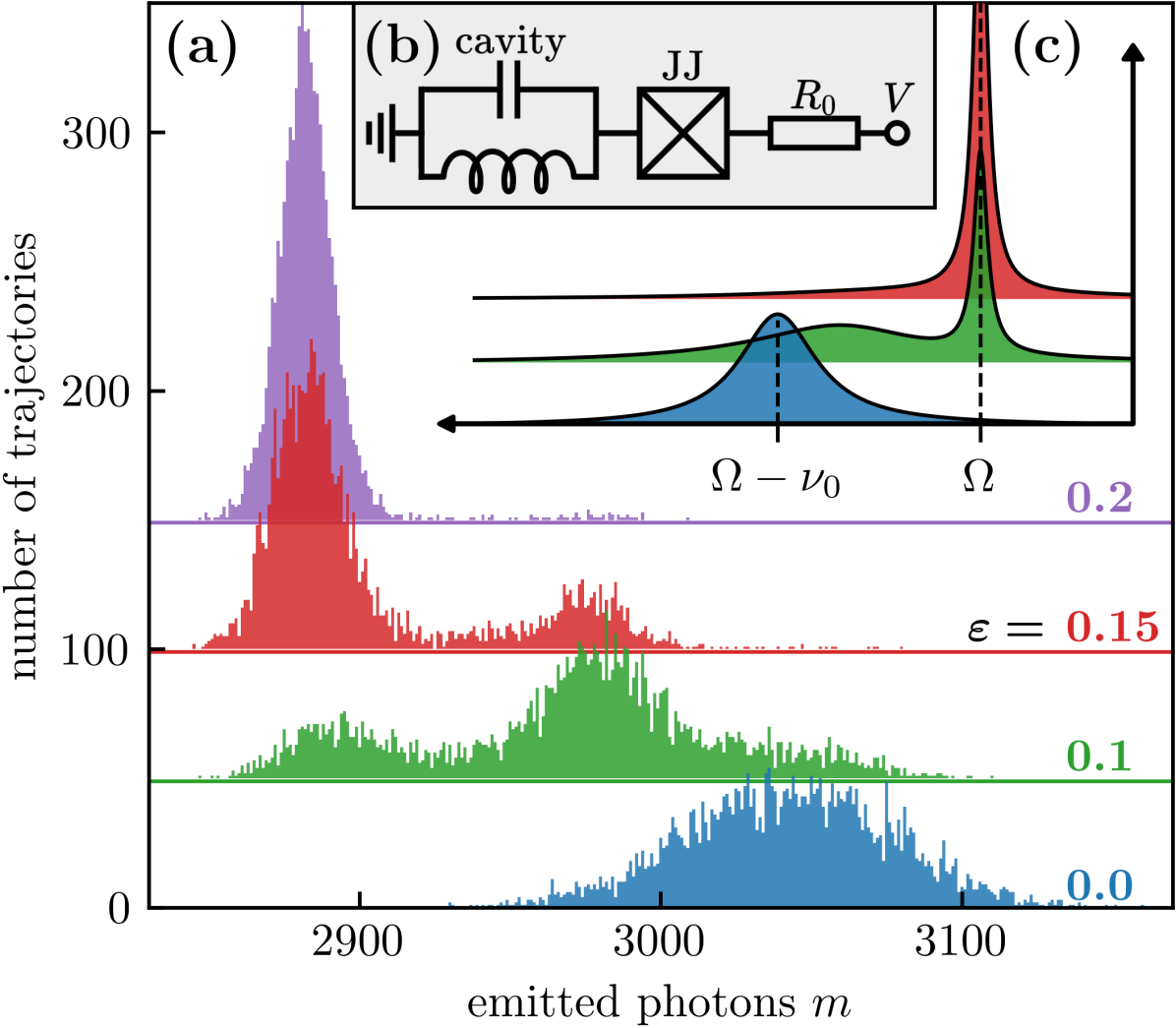
Figure 1: The microwave emission of a Josephson photonics device, consisting of a Josephson junction in-series to a microwave cavity and a resistance $R_{0}$ (b), can be locked by adding a small ac-signal (of strength $\varepsilon$ and frequency $\Omega$ on top of a dc-voltage drive. (c) Emission spectra $S(\omega)$ are centered around a frequency determined by the voltage across the junction but broadened by phase fluctuations. Applying a locking signal pulls the emission frequency towards $\Omega$, eventually resulting in a sharp emission peak at $\Omega$ [here artificially broadened by $\gamma/625$ (FWHM)]. (a) Histograms of photons emitted within at time interval $T=500/\gamma$. The photon statistics is directly linked to the statistics of voltage fluctuations and thus the spectral width. Increasing the locking strength narrows the photon emission statistics, while shot noise induces phase slips by $\Delta m=1/r_{0}$. [Parameters: $E_{J}^{*}/(\hbar\gamma)=4$, $\alpha=0.2$, $2eV_{\mathrm{dc}}/\hbar=\omega_{0}$, $\nu_{0}=0.02\gamma$, $r_{0}=1/100$, number of trajectories: 4000.]

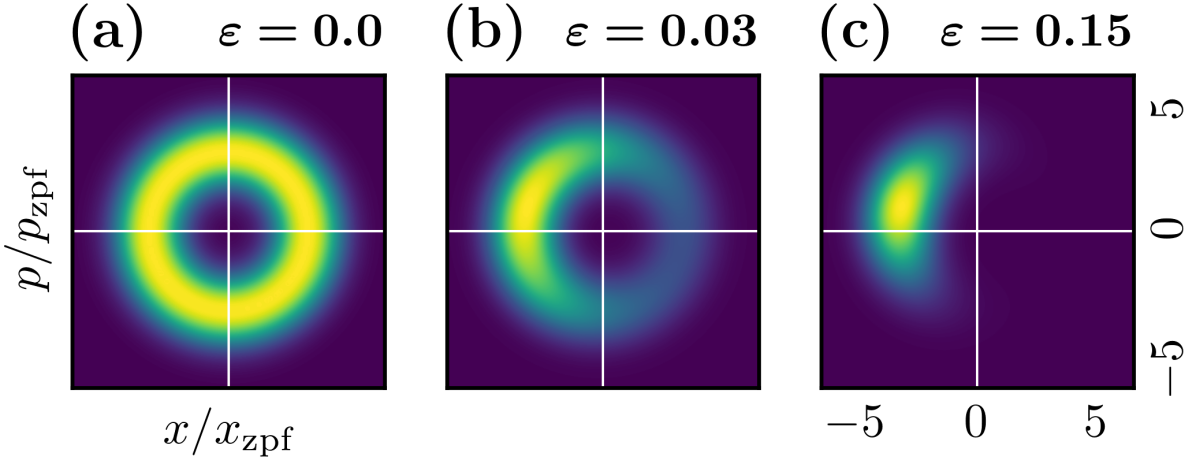
Figure 2: Wigner phase-space distributions of the cavity in the steady-state. (a) Without locking signal the shot noise diffuses the oscillator’s phase which becomes completely undefined. (c) The injection of a small ac-signal reduces the phase uncertainty, yielding a state with a sharply refocused phase in the locked regime. (b) In the intermediate regime shot noise and locking signal compete resulting in a state with partially diffused phase. [Parameters: $E_{J}^{*}/(\hbar\gamma)=3$, $\alpha=0.35$, $2eV_{\mathrm{dc}}/\hbar=\omega_{0}$, $\nu_{0}=0$, $r_{0}=1/50$. Wigner functions are normalized to their maxima.]

While, in general, the full quantum properties of the current operator $\hat{I}_{J}$ are difficult to obtain, we can make progress utilizing two observations. The integral expression determining the phase is proportional to the number of Cooper-pairs $m$ transferred across the junction in the elapsed time interval, so that the statistics of the voltage fluctuations is determined by the full counting statistics of Cooper pairs, and these were shown to match these of photons emitted from the cavity [43, 45]. This allows us to capture the voltage fluctuations on a resistance by an $m$-dependent c-number, $\varphi_{R_{0}}=2\pi r_{0}m$ where $r_{0}=R_{0}/R_{Q}$ is the in-series resistance in units of the superconducting resistance quantum $R_{Q}=h/(4e^{2})$, in the Hamiltonian (1), which is then used within an m-resolved quantum master equation or an equivalent quantum jump description. The model thus resembles a feedback-based locking scheme, where the in-series resistance realizes an autonomous adaptation of the driving phase to a measurement outcome. Technically, we use the standard method of number-resolved photon counting, where the density matrix, $\rho=\sum_{m=0}^{\infty}\rho_{m}$, is divided into components according to the number of photons $m$ leaked from the cavity after a time $t$. The components are coupled by photon jumps,

$$\dot{\rho}_{m}= -\frac{i}{\hbar}[H^{(m)}_{\mathrm{RWA}},\rho_{m}]+\frac{\gamma}{2}(2a\rho_{m-1}a^{\dagger}-a^{\dagger}a\rho_{m}-\rho_{m}a^{\dagger}a)$$ (2)

Non-standard, however, is the fact that the Hamiltonian itself becomes $m$-dependent:

$$\begin{split}&H^{(m)}_{\mathrm{RWA}}=\hbar(\omega_{0}-\Omega)a^{\dagger}a+\frac{E_{J}^{*}}{2}:\Bigg{[}ia^{\dagger}\frac{J_{1}(2\alpha\sqrt{a^{\dagger}a})}{\alpha\sqrt{a^{\dagger}a}}+\\ &\varepsilon\frac{J_{0}(2\alpha\sqrt{a^{\dagger}a})}{2\alpha}+\varepsilon a^{{\dagger}2}\frac{J_{2}(2\alpha\sqrt{a^{\dagger}a})}{2\alpha a^{\dagger}a}\Bigg{]}e^{i\psi(t,m)}+h.c.:\end{split}$$ (3)

with $\psi(t,m)=(\Omega t+\varphi_{\mathrm{ac}})-(2eV_{\mathrm{dc}}t/\hbar-2\pi r_{0}m)$. Here, we changed to a reference frame rotating with the frequency of the ac-signal $\Omega$ and in a rotating-wave approximation (RWA) neglected fast oscillating terms. The Josephson energy is renormalized, $E_{J}^{*}=E_{J}\alpha e^{-\alpha^{2}/2}$, and colons signal normal-ordering of the operators, cf. [40, 46].

Since the $m$-dependence of $H^{(m)}_{\text{RWA}}$ is periodic, there exists a natural compactification, when we chose (without loss of generality) $M=1/r_{0}\in\mathbb{N}$ and set $\rho_{M}=\rho_{0}$. This enables numerical simulations up to such times, that a very large number of photons has been emitted. With this method (and the quantum-regression theorem) the steady-state spectra of Fig. 1(c) discussed above are found.

Equivalently to the $m$-resolved quantum master equation (2), a jump approach can also be used [47], which replaces the Lindblad equation for the cavity density matrix $\rho$ with a stochastic equation of motion for a state vector $\ket{\psi}$. For each quantum trajectory the number of photons $m$ leaking from the cavity is counted and enters the Hamiltonian part of the dynamical equation as in Eq. (3). Resulting histograms for many simulated trajectories are shown in Fig. 1(a). When the external drive is absent, the distribution of counted photons is broad, conforming with a broad emission spectrum. An increase of the strength of the external locking signal reduces the width of the photon emission spectrum, and in the synchronized state the spectral width of the emitted photons is minimal.

Phase diffusion and its constraint by locking.—

The impact of the in-series resistance and resulting voltage fluctuations, and the locking signal can also be studied in a phase-space picture of the cavity dynamics. In Fig. 2 quantum-master equation results for the steady-state Wigner distribution are shown for different amplitudes of an injected ac-signal. The dc-voltage fixed close to resonance drives the cavity quickly into a (near coherent) state with finite amplitude. However, due to the lack of a reference phase, the imperfect dc-voltage drive across the junction disperses the phase of this state, until all information about the driving phase is lost in the steady state of the system [Fig. 2(a)]. The unstable phase-space angle is mirrored by the noise-induced broadening of the emission spectrum, cf. blue spectrum in Fig. 1(c). Turning on and increasing the amplitude of the ac-voltage, the completely dephased steady-state distribution contracts [Fig.  2(b-c)]. Concomitantly the variance of the phase-space angle is reduced and a sharpened peak emerges in the emission spectrum [cf. Fig. 1(c)]. Notably, in phase-space the effects of synchronization emerge completely smoothly with increasing strength $\varepsilon$, while the spectral pulling shows remnants of the classical criticality, see Fig. 1(c)] and Fig. 3(d) below.

We will understand and quantify the observed dynamics of the phase-space angle by linking it to the notion of constrained diffusion. For that purpose, we turn to the phase difference $\psi=(\Omega t+\varphi_{\mathrm{ac}})-(2eV_{\mathrm{dc}}t/\hbar-\varphi_{R_{0}})$ between the phase of the locking signal, $V_{\text{ac}}(t)=V_{\text{ac}}\cos[\Omega t+\varphi_{\text{ac}}]$, and the phase $2eV_{\text{dc}}t/\hbar-\varphi_{R_{0}}$ which drives the cavity. The synchronized state will then be characterized by a phase difference $\psi$ constant in time (modulo $2\pi$), since the cavity emits photons with frequencies centered sharply about the injection frequency $\Omega$. Equivalently, the photon count of a quantum-jump trajectory increases linearly in the synchronized regime as $m_{s}(t)\propto\varphi_{R_{0}}\sim(2eV_{\text{dc}}/\hbar-\Omega)t$. In Fig. 3(a) the deviations from this linear trend are shown for various coupling strengths. Deep in the synchronized state (green), deviations occur as short intervals of increased emission yielding stepwise increases between extended plateaus. While the latter correspond to a synchronized state, the former can be identified with phase slips: rapid changes of the phase difference by $2\pi$. How well a system is synchronized, can be quantified by the rate of such slips. Reducing the coupling (orange) accordingly increases the number of slips until the synchronized plateaus are completely absent (blue). The dependence of the phase slip rate on the locking strength in Fig. 3(d) shows a shot-noise induced broadening of the locking transition, compared to the noiseless, classical case ($r_{0}\rightarrow 0$) described by Adler-theory [48, 9, 38].

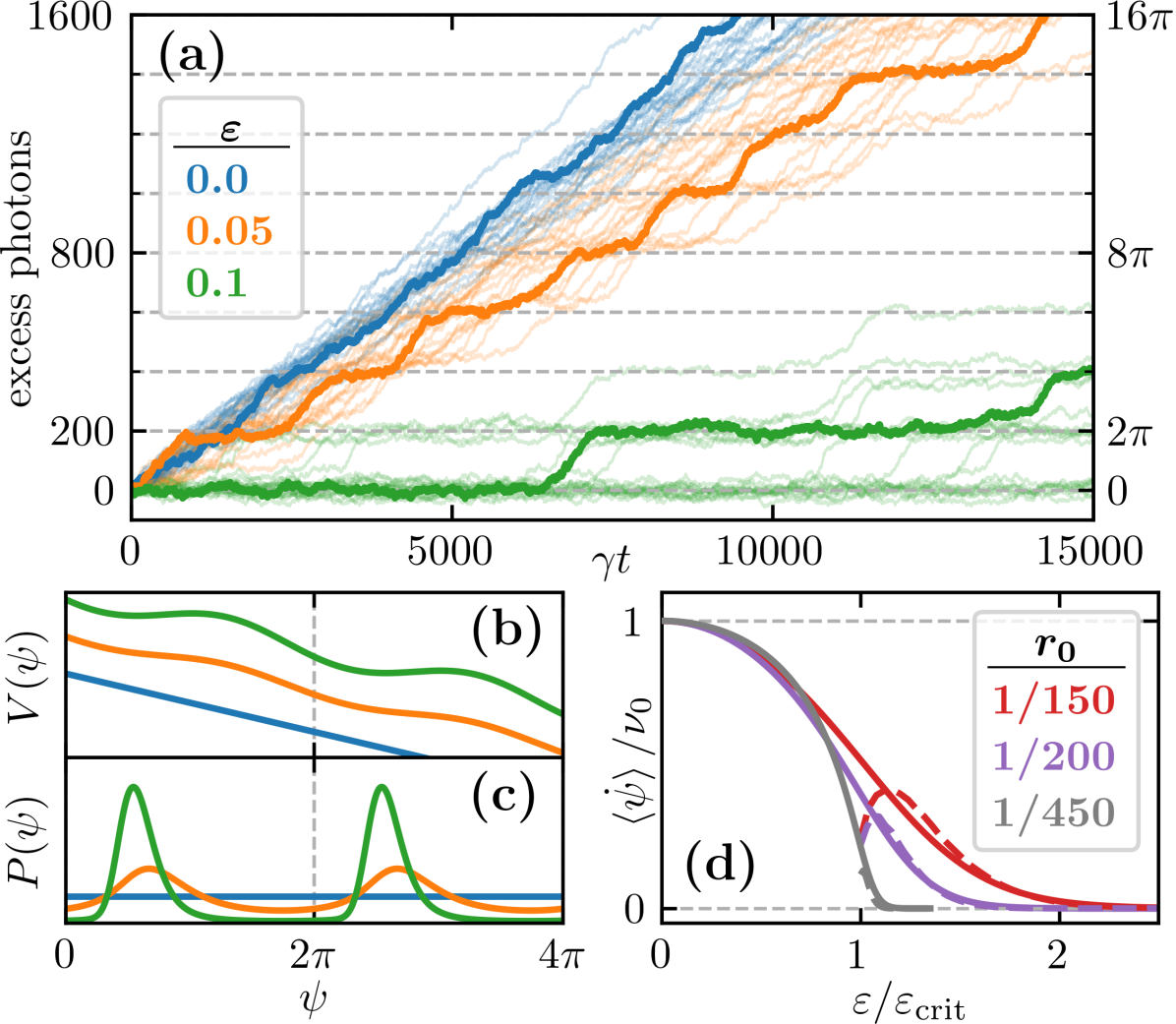
Figure 3: Photon emission records showing phase slips and reduced phase dynamics. (a) Emission records in the synchronized state (green) are characterized by long intervals with a well-defined emission rate, interrupted by bursts, wherein a fixed number of excess photons are emitted. These correspond to phase slips by $2\pi$, which proliferate (orange) and overlap (blue) in the unsynchronized regime. (b,c) The system dynamics can be reduced to diffusion dynamics of a phase $\psi$ in a tilted washboard-like potential. (d) At the locking transition the rate of phase slips $\langle\mathrm{d}\psi/\mathrm{d}t\rangle$ (solid), drops towards zero and the system is oscillating in synchronization with the locking signal. Phase slips can be approximated by an escape process (dashed). [Parameters: $E_{J}^{*}/(\hbar\gamma)=2.5$, $\alpha=0.35$, $2eV_{\mathrm{dc}}/\hbar=\omega_{0}$, $\nu_{0}=0.005\gamma$, $r_{0}=1/200$.]

Reduced dynamics of the phase.— The question that now arises is, whether a reduced equation for the dynamics of the phase variable $\psi$ can be derived in the quantum domain, thus generalizing the Adler-theory of classical synchronization dynamics [48, 9, 38]. Indeed, the number-resolved quantum-master equations, Eqs. (2) and (3), can be rewritten as an equation for a density $\rho^{\prime}(t,\psi)$ by first treating $m$ as continuous and transforming to a moving frame [49]. Crucially, the explicit time dependence of the Hamiltonian (3) is removed by the latter step. Assuming a time-scale separation between the (fast) adaptation of the cavity state to the phase of its driving term and the slow dynamics of the phase $\psi$, two-time perturbation theory can derive a Fokker-Planck equation for the dynamics on slow time scales $\tau=t\delta$ of the phase distribution probability [50, 51],

$$\partial_{\tau}P(\tau,\psi)=\partial_{\psi}\big{[}j(\psi)\,P(\tau,\psi)\big{]}+\frac{1}{2}\partial_{\psi}^{2}\big{[}D(\psi)\,P(\tau,\psi)\big{]},$$ (4)

valid in first-order of the perturbation parameter $\delta$ coupling slow and fast dynamics (cf. [52, 53] for applications in other number-resolved master equations).

While the full expressions for drift and diffusion term are involved (see Supplemental Material Eq. (S24) [49]), for the case without locking signal we find an equation describing free diffusion with diffusion constant $D=2\pi r_{0}S_{\mathrm{ph}}$ determined by the photonic shot noise power $S_{\mathrm{ph}}$ [54].

A numerical evaluation of the full expressions shows how the locking signal leads to a tilted washboard-potential, see Fig. 3(b), which develops local minima for sufficient locking strength. Accounting for the numerically gained diffusion $D(\psi)$, steady-state distributions of the phase shown in Fig. 3(c) can be found. The average flow of $\psi$ can also be calculated from the (steady-state) distribution and the drift (see Supplemental Material Eq. (S29) [49]) to gain the phase slip rate in Fig. 3(d). The dynamics of the phase can be approximated as an escape process with a Kramers-type rate $\sqrt{V^{{}^{\prime\prime}}_{m}V^{{}^{\prime\prime}}_{M}}e^{-\Delta V/(2D)}$ (dashed), where $\Delta V$ is the potential difference between the potential minimum $V_{m}$ and maximum $V_{M}$ and the prefactor is the geometric mean of the corresponding curvatures [55]. Without the shot noise, $D\equiv 0$, the reduced equation for the phase simplifies to the well-known Adler-equation describing the locking dynamics of a classical phase variable, $\mathrm{d}\psi/\mathrm{d}t=\nu_{0}+\nu_{c}\sin(\psi)$, where the classical parameters $\nu_{0}$ and $\nu_{c}$ emulate the numerical potentials $V(\psi)$ of Fig. 3(b). Diffusion in these potentials clearly links to the excess-photon traces of Fig. 3(a): with intra-potential diffusion matching the fluctuations within plateaus, and diffusion over the barriers corresponding to the phase slip steps.

Synchronization of two quantum microwave cavities.—Instead of the synchronization of a single nonlinearly driven microwave cavity to an external locking signal investigated above, one can also consider the mutual synchronization of several devices [9, 56]. Dispensing with the need of a phase-stable ac-signal, the prospect of mutual synchronization of a potentially large number of devices promises a source of correlated high-intensity emission. The Hamiltonian,

$$H=H_{a}+H_{b}+\epsilon(a^{\dagger}b+ab^{\dagger})\,\textrm{, where}$$ (5a)

$$\!\!H_{\xi}=\hbar\omega_{0}\xi^{\dagger}\xi-E_{J}\cos\!\!\left[\frac{2e}{\hbar}V_{\xi}t+\alpha(\xi^{\dagger}+\xi)-2\pi r_{0}m_{\xi}\right]\!\!\!$$ (5b)

describes a scenario (see inset of Fig. 4), where each device $\xi=a,b$ is biased by a dc-voltage $V_{\xi}$ applied across a resistance $R_{0}$, and the coupling term stems from a small coupling capacitor. We assume identical devices except for differing dc-voltage drives. The steady-state emission frequencies of the cavities, $\omega_{J,\xi}$, are by energy conservation arguments at vanishing coupling on average

$$\omega_{J,\xi}-\frac{2e}{\hbar}V_{\xi}=-2\pi r_{0}\gamma\braket{n_{\xi}}=-2\pi r_{0}\braket{\dot{m}_{\xi}}$$ (6)

which are in general detuned, $\nu=\omega_{J,b}-\omega_{J,a}\neq 0$. For nonzero coupling, $\epsilon\neq 0$, the first device will provide a reference frequency $\omega_{J,a}$ for the second device, which pulls the emission frequency of the second cavity $\omega_{J,b}$ towards the reference frequency, and vice versa. In the synchronized state, both cavities will emit photons about the same frequency, such that $\nu=0$. The joint photon counting statistics of the emission of the two cavities in the system’s steady state is shown in Fig. 4, with the marginal probability distributions in the side panels. For weak coupling (blue) the cavities are unsynchronized and the joint probability (approximately) factorizes into near-independent marginal probabilities [49]. The corresponding emission spectra will be broad and differ in their peak frequencies. For stronger coupling (red), the cavities are synchronized emitting around the same peak frequency, so that $\nu=0$ and $2\pi\hbar r_{0}\braket{m_{b}-m_{a}}/T=2e(V_{b}-V_{a})$. In the synchronized state, the statistics of the difference $m_{b}-m_{a}$ becomes extremely sharp compared to the marginal statistics of the single photon counts $m_{\xi}$. This number squeezing is accompanied by a merging and sharpening of the emission spectra of the two cavities ((Fig. 10 in Supplemental Material [49])). Notably, the strong correlation between the cavities is not associated with concomitant entanglement.

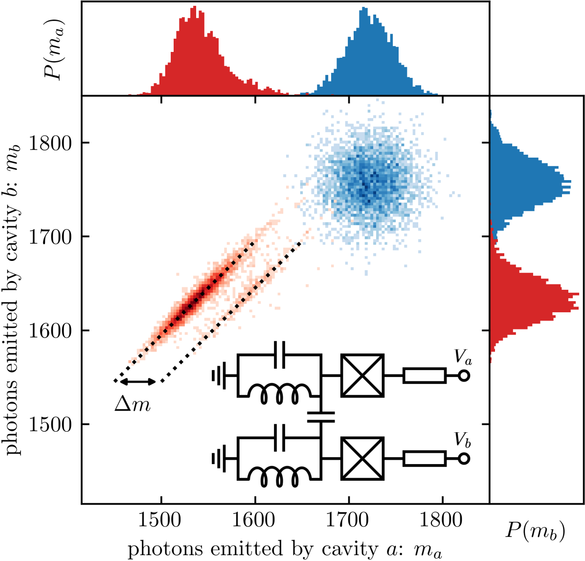
Figure 4: Joint photon emission statistics, $P(m_{a},m_{b})$, of two coupled Josephson-photonics systems (inset) in the synchronized (red) and unsynchronized (blue) regime with marginal probability distributions $P(m_{a})$ and $P(m_{b})$ shown in the upper and right side panels. In the synchronized state ($\epsilon/(\hbar\gamma)=0.12$), the statistics of the difference $m_{b}-m_{a}$ becomes extremely sharp with a sideband at distance $\Delta m=50$ indicating a slip of the relative phase by $2\pi$. [Parameters: $E_{J}^{*}/(\hbar\gamma)=3$, $\alpha=0.35$, $2eV_{a}/\hbar=\omega_{0}$, $2e(V_{b}-V_{a})/\hbar=0.02\gamma$, $r_{0}=1/50$, 4000 trajectories.]

Conclusion and outlook.— This Letter introduces dc-driven Josephson-photonics devices as a new platform to study quantum synchronization in the presence of shot-noise and the thereby induced phase slip dynamics. Mechanism and modeling of quantum synchronization dynamics in such devices differ from heretofore investigated systems and do not map to the paradigmatic case of a van der Pol oscillator. Nonetheless, the system can be reduced to its phase dynamics governed by a Fokker-Planck equation with a generalized Adler potential. Implementing synchronization in Josephson-photonics devices is of technological interest due their versatility as a source of quantum microwave light, but also promises fundamental insights in a deep quantum regime, where the nature of phase slips and the potential coexistence and interplay of charge and phase tunneling [57] can be studied.

We thank Andrew Armour, Benjamin Huard and Ambroise Peugeot for fruitful discussions and acknowledge the support of the DFG through AN336/17-1 and AN336/18-1 and the BMBF through QSens (project QComp).

Supplemental Material to "Quantum Synchronization in Presence of Shot Noise"

As supplemental material, we provide additional details on the derivation of the rotating-wave Hamiltonian and the change of reference frame for the phase and give a more quantitative discussion of spectral features. A detailed derivation of the Fokker-Planck equation for the reduced phase dynamics by two-time perturbation theory is also included, followed by a more extensive discussion of its solution. Finally more details on synchronizing two cavities and particularly the spectral signatures of these phenomena are given.

I Rotating-wave Hamiltonian

The Hamiltonian of the dc-biased Josephson-photonics device with in-series resistance $R_{0}$ and injection locking signal ${V(t)=V_{\mathrm{dc}}+V_{\mathrm{ac}}\cos(\Omega t+\varphi_{\mathrm{ac}})}$ is

$$H=\hbar\omega_{0}a^{\dagger}a-E_{J}\cos\left[\alpha(a^{\dagger}+a)+\omega_{\mathrm{dc}}t+\varepsilon\sin(\Omega t+\varphi_{\mathrm{ac}})-\varphi_{R_{0}}\right],$$ (S1)

where $\omega_{\mathrm{dc}}=2eV_{\mathrm{dc}}/\hbar$ and $\varepsilon=2eV_{\mathrm{ac}}/(\hbar\Omega)$ We transform the Hamiltonian to a reference frame rotating at $\omega_{\mathrm{rf}}\approx\omega_{\mathrm{dc}}$ using the unitary operator $U=e^{i\omega_{\mathrm{rf}}ta^{\dagger}a}$. Linearizing the expression in $\varepsilon$

$$\begin{split}H_{\mathrm{rf}}=UHU^{\dagger}+i\hbar\dot{U}U=\hbar(\omega_{0}-\omega_{\mathrm{rf}})a^{\dagger}a-\frac{E_{J}}{2}\Big{\{}&\left[1+i\varepsilon\sin(\Omega t+\varphi_{\mathrm{ac}})\right]e^{i(\omega_{\mathrm{dc}}t-\varphi_{R_{0}})}e^{i\alpha(a^{\dagger}+a)}\\ &\times e^{i\alpha\exp(i\omega_{\mathrm{rf}}t)a^{\dagger}}e^{i\alpha\exp(-i\omega_{\mathrm{rf}}t)a}+\textrm{h.c.}\Big{\}}.\end{split}$$ (S2)

Finally, we perform a rotating wave approximation where we only keep slowly oscillating terms

$$\begin{split}H_{\mathrm{RWA}}=\hbar(\omega_{0}-\omega_{\mathrm{rf}})a^{\dagger}a+\frac{E_{J}^{*}}{2}:&(ie^{-i(\omega_{\mathrm{dc}}t-\varphi_{R_{0}}-\omega_{\mathrm{rf}}t)}a^{\dagger}+h.c.)\frac{J_{1}(2\alpha\sqrt{a^{\dagger}a})}{\alpha\sqrt{a^{\dagger}a}}\\ &+\frac{\varepsilon}{2}(e^{-i(\Omega t+\varphi_{\mathrm{ac}}+\omega_{\mathrm{dc}}t-\varphi_{R_{0}}-2\omega_{\mathrm{rf}})}a^{{\dagger}2}+\textrm{h.c.})\frac{J_{2}(2\alpha\sqrt{a^{\dagger}a})}{\alpha a^{\dagger}a}\\ &+\frac{\varepsilon}{2}(e^{-i(-\Omega t-\varphi_{\mathrm{ac}}+\omega_{\mathrm{dc}}t-\varphi_{R_{0}})}+\textrm{h.c.})\frac{J_{0}(2\alpha\sqrt{a^{\dagger}a})}{\alpha}:\end{split}$$ (S3)

with the renormalized Josephson energy $E_{J}^{*}=E_{J}\alpha e^{-\alpha^{2}/2}$. Setting $\omega_{\mathrm{rf}}t\rightarrow\Omega t+\varphi_{\mathrm{ac}}$ the rotating frame yields Eq. (3) in the main text.

II Phase in a moving reference frame

We write Eq. (2) of the main text in terms of the phase $\varphi_{R_{0}}=2\pi r_{0}m$ instead of the number $m$ of photons leaked from the cavity and treat $\varphi_{R_{0}}$ as a continuous quantity. With $\rho(t,\varphi_{R_{0}}=2\pi r_{0}m)=\rho_{m}(t)$, we get

$$\frac{\partial\rho}{\partial t}(t,\varphi_{R_{0}})=-\frac{i}{\hbar}\left[H_{\text{RWA}}(t,\varphi_{R_{0}}),\rho(t,\varphi_{R_{0}})\right]+\frac{\gamma}{2}\left[2a\rho(t,\varphi_{R_{0}}-2\pi r_{0})a^{\dagger}-a^{\dagger}a\rho(t,\varphi_{R_{0}})-\rho(t,\varphi_{R_{0}})a^{\dagger}a\right].$$ (S4)

We want to express $\varphi_{R_{0}}$ in terms of a phase $\psi$ in a moving reference frame, which is defined by the transformation

$$\varphi_{R_{0}}(t,\psi)=\psi+\omega_{\mathrm{dc}}t-(\Omega t+\varphi_{\mathrm{ac}}).$$ (S5)

Accordingly, the density matrix becomes a new function of $t$ and $\psi$

$$\rho^{\prime}(t,\psi)=\rho\big{(}t,\varphi_{R_{0}}(t,\psi)\big{)}$$ (S6)

with the time derivative

$$\frac{\partial\rho^{\prime}}{\partial t}(t,\psi)=\frac{\mathrm{d}\rho}{\mathrm{d}t}\big{(}t,\varphi_{R_{0}}(t,\psi)\big{)}=\frac{\partial\rho}{\partial t}\big{(}t,\varphi_{R_{0}}(t,\psi)\big{)}+\frac{\partial\rho}{\partial\varphi_{R_{0}}}\big{(}t,\varphi_{R_{0}}(t,\psi)\big{)}\frac{\partial\varphi_{R_{0}}}{\partial t}(t,\psi).$$ (S7)

Using Eq. (S4) we can rewrite the right-hand side of this equation giving

$$\begin{split}\frac{\partial\rho^{\prime}}{\partial t}(t,\psi)&=-\frac{i}{\hbar}\Big{[}H^{\prime}_{\mathrm{RWA}}(\psi),\rho^{\prime}(t,\psi)\Big{]}+\frac{\gamma}{2}\Big{[}2a\rho^{\prime}(t,\psi-2\pi r_{0})a^{\dagger}-a^{\dagger}a\rho^{\prime}(t,\psi)-\rho^{\prime}(t,\psi)a^{\dagger}a\Big{]}+(\omega_{\mathrm{dc}}-\Omega)\frac{\partial\rho^{\prime}}{\partial\psi}(t,\psi)\\ &=:\Lambda(\psi)\rho^{\prime}(t,\psi)\end{split}$$ (S8)

introducing the evolution generator $\Lambda(\psi)$. With the rotating frame Hamiltonian from Eq. (3) in the main text, the Hamiltonian $H^{\prime}_{\mathrm{RWA}}(\psi)=H_{\mathrm{RWA}}(t,\varphi_{R_{0}}(t,\psi))$ does not have an explicit time dependence.

III Details on the emission spectra

To calculate the emission spectra we evolve the system to a time $t_{0}$ to reach its steady-state and determine the correlation function $\braket{a^{\dagger}(t)a(t_{0})}$ with the corresponding spectrum

$$S(\omega)=\frac{1}{\sqrt{2\pi}}\int_{-\infty}^{\infty}\braket{a^{\dagger}(t)a(t_{0})}e^{-i\omega(t-t_{0})}\mathrm{d}t\,.$$ (S9)

As seen in Fig. 1 of the main text, the spectrum has a wide part and one $\delta$-peaked part, which is artificially broadened in that figure for presentation purposes. In Fig. 5 the areas $A_{\mathrm{broad}}$ and $A_{\delta}$ below these curves are shown, demonstrating how spectral weight shifts to the $\delta$-part of the spectrum as the system locks onto $\Omega$. The sum $A_{\mathrm{broad}}+A_{\delta}=\braket{a^{\dagger}(t_{0})a(t_{0})}$ changes slightly with the strength $\varepsilon$ of the locking signal as the frequency gets pulled.

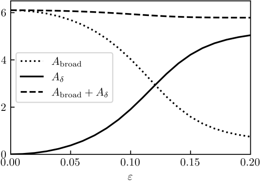
Figure 5: Spectral contribution of the broad part $A_{\mathrm{broad}}$ and $\delta$-peak $A_{\delta}$. The total emission changes with $\varepsilon$ as the frequency gets pulled. [Parameters see Fig. 1]

IV Derivation of the Fokker-Planck equation by two-time perturbation theory

We perform two-time scale perturbation theory (or homogenisation) to derive an effective Fokker-Plank equation for the phase $\psi$. For that purpose it is assumed that the oscillator dynamics takes place on a much faster time scale than the phase dynamics. We also assume that $r_{0}$ and $(\omega_{\text{dc}}-\Omega)/\gamma$ are of the same order and rescale them $r_{0}\rightarrow\delta r_{0}$, $\omega_{\text{dc}}-\Omega\rightarrow\delta(\omega_{\text{dc}}-\Omega)$ by the dimensionless parameter $\delta\ll 1$. We explicitly introduce a fast time scale $t$ and a slow time scale $\tau=t\delta$ and the dependence of the state on these times $\rho^{\prime}(t,\psi)=\rho(t,\tau,\psi)$. The time derivative of the density matrix in Eq. (S8) $\partial\rho^{\prime}(t,\psi)/\partial t$ then becomes

$$\frac{\mathrm{d}}{\mathrm{d}t}\rho(t,\tau,\psi)=\partial_{t}\rho(t,\tau,\psi)+(\partial_{t}\tau)\partial_{\tau}\rho(t,\tau,\psi)=\partial_{t}\rho(t,\tau,\psi)+\delta\partial_{\tau}\rho(t,\tau,\psi).$$ (S10)

Furthermore, we assume that the fast oscillator dynamics have already relaxed and we study the evolution of the state

$$\rho(\tau,\psi)=\lim_{t\rightarrow\infty}\rho(t,\tau,\psi).$$ (S11)

The resulting equation of motion

$$\delta\partial_{\tau}\rho(\tau,\psi)=\Lambda(\psi)\rho(\tau,\psi),$$ (S12)

c.f. Eq. (S8), is now to be expanded in orders of $\delta$. Firstly, the expansion of the generator of the evolution $\Lambda(\psi)$ yields

$$\Lambda(\psi)=\sum_{k=0}^{\infty}\delta^{k}\frac{\partial_{\psi}^{k}}{k!}\Lambda^{(k)}$$ (S13)

with

$$\Lambda^{(0)}\rho(\tau,\psi)=-\frac{i}{\hbar}[H_{\text{RWA}}(\psi),\rho(t,\psi)]+\frac{\gamma}{2}\left[2a\rho(t,\psi)a^{\dagger}-a^{\dagger}a\rho(t,\psi)-\rho(t,\psi)a^{\dagger}a\right]$$ (S14)

$$\Lambda^{(1)}\rho(\tau,\psi)=(\omega_{\text{dc}}-\Omega)\rho(\tau,\psi)-2\pi r_{0}\gamma a\rho(\tau,\psi)a^{\dagger},\qquad\Lambda^{(k>1)}\rho(\tau,\psi)=(-2\pi r_{0})^{k}\gamma a\rho(\tau,\psi)a^{\dagger}.$$ (S15)

Secondly, we also expand the state

$$\rho(\tau,\psi)=\sum_{k=0}^{\infty}\delta^{k}\rho^{(k)}(\tau,\psi).$$ (S16)

Using these expansion we can now proceed solving Eq. (S12) order by order.

In 0th order we find

$$\Lambda^{(0)}\rho^{(0)}(\tau,\psi)=0$$ (S17)

which can be solved by $\rho^{(0)}(\tau,\psi)=P^{(0)}(\tau,\psi)\rho_{\text{eq}}(\psi)$, where $P^{(0)}(\tau,\psi)$ is a time (and $\psi$) dependent weight of $\rho_{\mathrm{eq}}$. For each $\psi$ the density matrix $\rho_{\mathrm{eq}}$ is normalized $\mathrm{tr}\left[\rho_{\mathrm{eq}}(\psi)\right]=1\;\forall\psi$.
Physically, the state $\rho_{\mathrm{eq}}(\psi)$ is the steady state of a damped oscillator driven by the nonlinear Josephson photonics term in a direction in phase space determined by the phase $\psi$. Changing $\psi$ does not merely rotate that state due to the additional $\varepsilon$-dependent terms in Eq. (3). To determine the 0th-order weight $P^{(0)}(\tau,\psi)$ we must advance to the next order.

In 1st order,

$$\delta\partial_{\tau}\rho^{(0)}=\delta\Lambda^{(0)}\rho^{(1)}+\delta\partial_{\psi}(\Lambda^{(1)}\rho^{(0)}).$$ (S18)

Tracing over the quantum degrees of freedom and using the fact that $\Lambda^{(0)}$ is a (trace-preserving) Lindbladian, we find the (partial) differential equation determining $P^{(0)}$

$$\partial_{\tau}P^{(0)}(\tau,\psi)=\partial_{\psi}\text{tr}\left[\Lambda^{(1)}\rho_{\text{eq}}P^{(0)}(\tau,\psi)\right].$$ (S19)

Furthermore, let $V_{n}$ be the left and $W_{n}$ be the right eigenoperators of $\Lambda^{(0)}$ with eigenvalues $\lambda_{n}$, with $V_{0}=1$, $W_{0}=\rho_{\text{eq}}$ and $\lambda_{0}=0$. Note that all eigenoperators and eigenvalues implicitly depend on $\psi$. Taking the Hilbert-Schmidt inner product on both sides of (S21) then gives

$$\text{tr}(V^{\dagger}_{n}\rho^{(1)}(\tau,\psi))=-\frac{1}{\lambda_{n}}\text{tr}\left\{V_{n}^{\dagger}\Lambda^{(1)}\partial_{\psi}\left[\rho_{\text{eq}}P^{(0)}(\tau,\psi)\right]\right\}\quad\text{for}\quad n\neq 0.$$ (S20)

As encountered in the lowest order, the first order density matrix $\rho^{(1)}$ is not completely determined by the projections on $V_{n\neq 0}$ in Eq. (S20). Namely, the (first-order) weight, $P_{1}=\mathrm{tr}\rho^{(1)}=\mathrm{tr}(V_{0}^{\dagger}\rho^{(1)})$, is the projection on $V_{0}$ excluded in Eq. (S20) and has to be found by the next order of the expansion.

The 2nd order equation is

$$\partial_{\tau}\rho^{(1)}(\tau,\psi)=\Lambda^{(0)}\rho^{(2)}(\tau,\psi)+\partial_{\psi}\Lambda^{(1)}\rho^{(1)}(\tau,\psi)+\frac{1}{2}\partial^{2}_{\psi}\Lambda^{(2)}\rho^{(0)}(\tau,\psi)$$ (S21)

and taking the trace we find

$$\partial_{\tau}P^{(1)}(\tau,\psi)=\partial_{\psi}\text{tr}\left[\Lambda^{(1)}\rho^{(1)}(\tau,\psi)\right]+\frac{1}{2}\partial^{2}_{\psi}\text{tr}\left[\Lambda^{(2)}\rho^{(0)}(\tau,\psi)\right].$$ (S22)

We can rewrite the first term of the right-hand side using the completeness of the left and right eigenoperators, $\mathrm{tr}(\Lambda^{(1)}\rho^{(1)})=\sum_{n=0}\mathrm{tr}(V_{n}^{\dagger}\rho^{(1)})\mathrm{tr}(\Lambda^{(1)}W_{n})$, so that Eq. (S20) can be used. In that manner, we find as a central result, that $P=P^{(0)}+\delta P^{(1)}$ solves the Fokker-Planck equation

$$\partial_{\tau}P(\tau,\psi)=\partial_{\psi}\Big{\{}\left[j^{(0)}(\psi)+\delta j^{(1)}(\psi)\right]P(\tau,\psi)\Big{\}}+\delta\frac{1}{2}\partial_{\psi}^{2}\Big{\{}D(\psi)\,P(\tau,\psi)\Big{\}}$$ (S23)

with

$$j^{(0)}(\psi)= \text{tr}\left[(\omega_{\text{dc}}-\Omega-2\pi r_{0}\gamma a^{\dagger}a)\rho_{\text{eq}}\right]$$ (S24a)

$$j^{(1)}(\psi)= -\sum_{n=1}\text{tr}\left(2\pi r_{0}\gamma a^{\dagger}aW_{n}\right)\text{tr}\left\{\left(\partial_{\psi}\frac{V_{n}^{\dagger}}{\lambda_{n}}\right)\left[(\omega_{\text{dc}}-\Omega)\rho_{\text{eq}}-2\pi r_{0}\gamma a\rho_{\text{eq}}a^{\dagger}\right]\right\}$$

$$+\sum_{n=1}\text{tr}\left(2\pi r_{0}\gamma a^{\dagger}a\partial_{\psi}W_{n}\right)\text{tr}\left(\frac{V_{n}^{\dagger}}{\lambda_{n}}2\pi r_{0}\gamma a\rho_{\text{eq}}a^{\dagger}\right)$$ (S24b)

$$D(\psi)= (2\pi r_{0})^{2}\gamma\,\text{tr}\left(a\rho_{\text{eq}}a^{\dagger}\right)-2\sum_{n=1}\text{tr}\left(2\pi r_{0}\gamma a^{\dagger}aW_{n}\right)\text{tr}\left(\frac{V_{n}^{\dagger}}{\lambda_{n}}2\pi r_{0}\gamma\ a\rho_{\text{eq}}a^{\dagger}\right).$$ (S24c)

The drift and diffusion constants $j(\psi)=j^{(0)}(\psi)+j^{(1)}(\psi)$ and $D(\psi)$ are shown in Fig. 6.
For weak driving, i.e. small $E_{J}^{*}$, the equilibrium state $\rho_{eq}$ is close to a coherent state. Therefore in this limit the second terms of $j^{(1)}(\psi)$ and $D(\psi)$ vanish and $D(\psi)\propto\gamma\langle a^{\dagger}a\rangle_{\textrm{eq}}$. Furthermore, for small $E_{J}^{*}$ the dependence of $\rho_{eq}$ on $\psi$ will be weak which means also the first term of $j^{(1)}(\psi)$ disappears.
In the absence of the locking signal, i.e. when $\varepsilon=0$, $j^{(0)}$, $j^{(1)}$ and $D$ are $\psi$ independent. This can readily be seen by transforming $\Lambda^{(0)}$ Eq. (S14) with the unitary $U=e^{ia^{\dagger}a\psi}$, which removes all $\psi$ dependence from the expansion. Furthermore, the traces in Eqs. (S24) are invariant under $U$. The diffusion constant is then proportional to the shot noise of the photon flow of the dc-driven system, which also equals the noise of the Cooper-pair current [43, 45, 54].

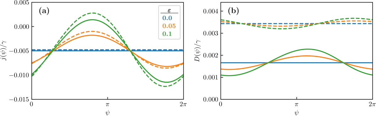
Figure 6: Drift and diffusion parameters of the Fokker-Planck equation for the slow-time diffusion of the phase $\psi$, Eq. (S24) for various values of the locking strength $\epsilon$ (solid line: full expressions, dashed: only $j^{(1)}$ and first term of $D$). (a) Without locking signal (blue) the phase moves in a linearly tilted potential $V(\psi)$ resulting in a constant drift, $j\propto\partial_{\psi}V(\psi)$, while increasing $\varepsilon$ yields the familiar tilted-washboard potential (orange) which develops extrema, $j(\psi)=0$, in the locked regime (green). (b) The diffusion is nearly uniform in $\psi$ with small variations which increase with $\varepsilon$. [Parameters see Fig. 3]

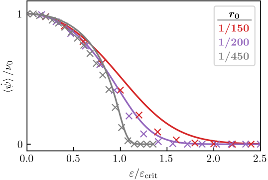
Figure 7: Rate of phase slips comparing the results of the $m$-resolved master equation (crosses) and Fokker-Planck equation. For small values of $\tilde{R_{0}}$ the curves correspond well, as the Fokker-Planck equation only keeps terms up to second order in $r_{0}$. [Parameters see Fig. 3]

V Interpretation and steady-state solution of the Fokker-Planck equation

The Fokker-Planck equation (S23) describes the motion of an overdamped particle at the position $\psi$

$$\dot{\psi}=-j(\psi)+\Gamma(\tau,\psi)$$ (S25)

with a random force $\Gamma(\tau,\psi)$ acting on it. The drift term $j(\psi)$ corresponds to a potential

$$V(\psi)=\int j(\psi)\mathrm{d}\psi$$ (S26)

as shown on Fig. 3(b). For an exclusively dc-driven system the potential is a tilted straight line. Increasing the amplitude $\varepsilon$ of the ac-locking signal creates modulations of the drift and diffusion constants in the phase $\psi$, resulting in a tilted-washboard potential.
If we compactify the phase $\psi$ and identify $0$ and $2\pi$, the Fokker-Planck equation (S23) has a steady state solution given by [55]

$$P_{\mathrm{ss}}(\psi)=Ne^{-\Phi(\psi)}\left[1-C\int_{0}^{\psi}\frac{e^{\Phi(\xi)}}{2D(\xi)}\mathrm{d}\xi\right],$$ (S27)

where

$$\Phi(\psi)=\log[2D(\psi)]+\int_{0}^{\psi}\frac{j(\xi)}{2D(\xi)}\mathrm{d}\xi.$$ (S28)

The integration constants $N$ and $C$ are determined by normalization and the periodic boundary condition $P_{\mathrm{ss}}(0)=P_{\mathrm{ss}}(2\pi)$. As expected, $P_{\mathrm{ss}}(\psi)$ shows a strong localization in the minima of the washboard potential, see Fig. 3(c).
The mean drift of the phase $\psi$ can be determined according to

$$\braket{\dot{\psi}}=-\int_{0}^{2\pi}P_{\mathrm{ss}}(\psi)j(\psi)\mathrm{d}\psi,$$ (S29)

which yields the frequency pulling curve in Fig. 3(d). Fig. 7 compares the results of the Fokker-Planck equation to the full numerics of the $m$-resolved master equation. As the Fokker-Planck equation is a differential equation of second-order in $\psi$, it neglects terms of higher order than $r_{0}^{2}$. Therefore, it is a particularly good description for small $r_{0}$, which is convenient because numerical simulations (both quantum jump and master-equation) become computationally costly in this limit.

VI Details on the synchronization of two cavities

As explained and demonstrated in the main text, see e.g. Fig. 4, two coupled Josephson-photonics cavities can synchronize their oscillations. Fig. 8(a) explicitly demonstrates a statement, that was gained by inspection of Fig. 4, namely, that in the unsynchronized regime the cavities emit independently, so that the joint probability distribution factorizes, $P(m_{a},m_{b})=P(m_{a})P(m_{b})$, while in the synchronized state, there are strong correlations and a sharp distribution for the difference of counts.

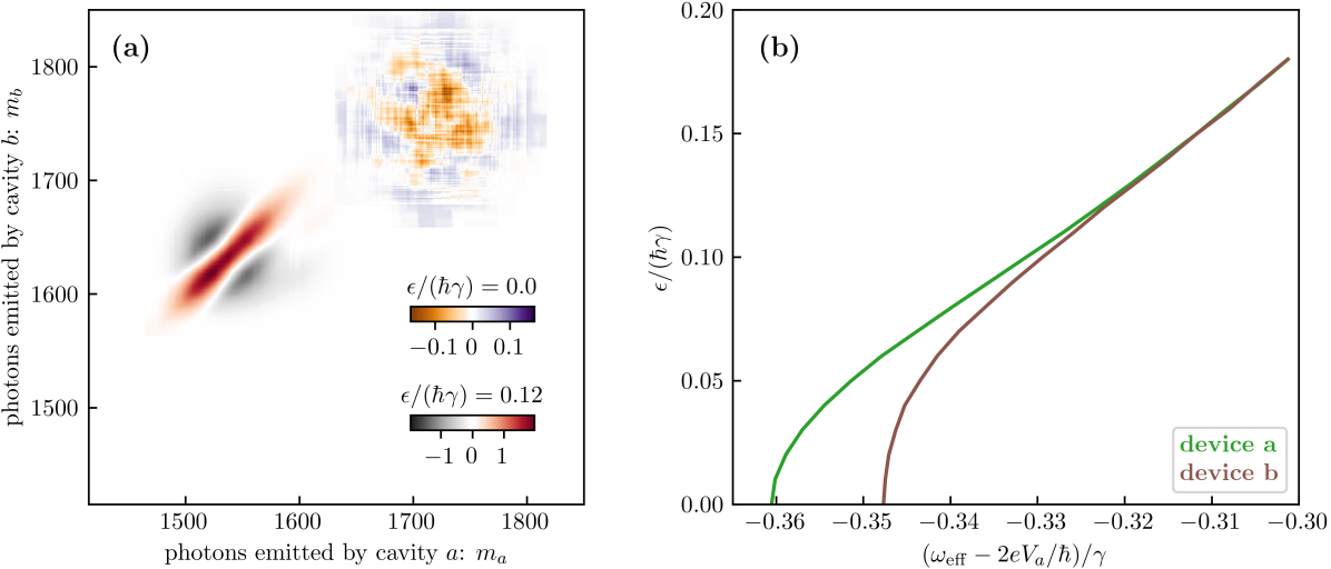
Figure 8: (a) Correlations of the photon-emission counts from two cavities, $a,\,b$, cf. Fig. 4 of the main text based on the same data. If the two devices are uncoupled (blue-orange colors, $\epsilon\equiv 0$) the joint probability $P(m_{a},m_{b})=P(m_{a})P(m_{b})$ is given by the product of the marginal probabilities and the deviations $P(m_{a},m_{b})-P(m_{a})P(m_{b})$ shown are small (Distributions are gained from 4000 trajectories and smoothed with a running mean of 30). The pronounced structures in the synchronized state (red-black colors, $\epsilon/(\hbar\gamma)=0.12$) indicate strong correlations. (b) The effective driving frequencies, $\omega_{\mathrm{eff},a}=2eV_{a}/\hbar-2\pi r_{0}\gamma\braket{a^{\dagger}a}$ and $\omega_{\mathrm{eff},b}=2eV_{b}/\hbar-2\pi r_{0}\gamma\braket{b^{\dagger}b}$ of two Josephson photonics devices are pulled towards each other and synchronize if the coupling $\epsilon$ is increased. The emission also peaks at these frequencies, see Fig. 9. [Parameters as in Fig. 4]

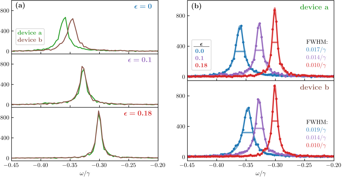
Figure 9: Microwave emission spectra for two coupled Josephson photonics devices. (a) Bias voltages are chosen slightly differently, so that the emission spectra of the individual devices are distinct for $\epsilon=0$. Increasing the coupling pulls the peaks of the spectra together, c.f. Fig. 8(b). (b) As a consequence of the restricted phase diffusion, the width of the spectra is also reduced, which is shown by the FWHM of a Lorentzian fit. [Parameters as in Fig. 4]

It is important to clarify the distinction between the strong correlations induced by synchronization, which in essence are classical correlations, and quantum mechanical entanglement. Indeed, we can characterize the entanglement of our system by its logarithmic negativity defined as $E_{N}(\rho)=\log_{2}||\rho^{\Gamma_{a}}||_{1}$ where $||\cdot||$ is the trace norm of the density matrix which is partially transposed with respect to the subsystem a. Generally, one may expect to find some entanglement, which increases with the strength of the coupling between the two systems. Here, in fact, this is only the case for a perfect voltage source ($r_{0}=0$, and hence no synchronization), where one finds a small degree of entanglement, while for non-zero resistance, $r_{0}=1/50$, this entanglement vanishes. Hence, the strong correlations of $m_{a}$ and $m_{b}$ are clearly distinct from entanglement.

Increasing the coupling $\epsilon$ synchronizes the devices, but also reduces the voltage drop at the resistance $R_{0}$. Using the four-wave Monte-Carlo technique [58] we also obtained the full spectral distribution of the cavity emission. Synchronization is reflected in the spectra in Fig. 9(a) by the fact that the peaks of the emission are pulled together in the same way as the effective driving frequencies in Fig. 8(b). A fit with a Lorentzian Fig. 9(b) reveals that also the linewidth of the emission is reduced by synchronizing the devices. At first, this might be surprising as the distribution of the driving phases $\varphi_{a}=\left(2eV_{a}t/\hbar-2\pi r_{0}m_{a}\right)$ and $\varphi_{b}=\left(2eV_{b}t/\hbar-2\pi r_{0}m_{b}\right)$ are also wide in synchronized state, see Fig. 4. It can, however, be understood describing the problem in terms of sum and difference variables

$$\eta=\varphi_{b}+\varphi_{a}\qquad\mathrm{and}\qquad\psi=\varphi_{b}-\varphi_{a}.$$ (S30)

By utilizing two-time perturbation-theory in analog to Supplemental Material IV one arrives at a two-dimensional Fokker-Planck equation

$$\partial_{\tau}P=\partial_{\eta}\left(j_{\eta}P\right)+\partial_{\psi}\left(j_{\psi}P\right)+\frac{1}{2}\partial_{\eta}^{2}(D_{\eta}P)+\partial_{\eta}\partial_{\psi}(D_{\eta\psi}P)+\frac{1}{2}\partial_{\psi}^{2}(D_{\psi}P).$$ (S31)

The shot noise in $m_{a}$ and $m_{b}$ gives rise to the diffusion constants where the mixed term $D_{\eta\psi}$ indicates correlated noise in $\eta$ and $\psi$. The drift terms with the constants $j_{\eta}$ and $j_{\psi}$ correspond to a two-dimensional tilted-washboard potential determined via

$$\partial_{\eta}V(\eta,\psi)=j_{\eta}\qquad\mathrm{and}\qquad\partial_{\psi}V(\eta,\psi)=j_{\psi}.$$ (S32)

A sketch of this potential for zero detuning $V_{a}=V_{b}$ is given in Fig. 10. The probability distribution of the phase diffuses freely in $\eta$-direction, whereas diffusion in direction of the difference variable $\psi$ is constrained by the washboard potential and does not contribute to spectral broadening. In consequence, diffusion in $\varphi_{a}$ ($\varphi_{b}$) -direction is reduced and the spectra narrowed.

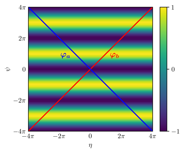
Figure 10: Sketch of the two-dimensional washboard potential for $V_{a}=V_{b}$. The potential restricts diffusion in $\psi$-direction while there is no restriction in $\eta$ direction. Hence, diffusion in $\varphi_{a}$ and $\varphi_{b}$-direction is also reduced.

References

- Hofheinz et al. [2011] M. Hofheinz, F. Portier, Q. Baudouin, P. Joyez, D. Vion, P. Bertet, P. Roche, and D. Estève, Bright side of the coulomb blockade, Phys. Rev. Lett. 106, 217005 (2011).
- Peugeot et al. [2021] A. Peugeot, G. Ménard, S. Dambach, M. Westig, B. Kubala, Y. Mukharsky, C. Altimiras, P. Joyez, D. Vion, P. Roche, et al., Generating two continuous entangled microwave beams using a dc-biased josephson junction, Physical Review X 11, 031008 (2021).
- Ménard et al. [2022] G. C. Ménard, A. Peugeot, C. Padurariu, C. Rolland, B. Kubala, Y. Mukharsky, Z. Iftikhar, C. Altimiras, P. Roche, H. le Sueur, P. Joyez, D. Vion, D. Esteve, J. Ankerhold, and F. Portier, Emission of photon multiplets by a dc-biased superconducting circuit, Phys. Rev. X 12, 021006 (2022).
- Grimm et al. [2019] A. Grimm, F. Blanchet, R. Albert, J. Leppäkangas, S. Jebari, D. Hazra, F. Gustavo, J.-L. Thomassin, E. Dupont-Ferrier, F. Portier, and M. Hofheinz, Bright on-demand source of antibunched microwave photons based on inelastic cooper pair tunneling, Phys. Rev. X 9, 021016 (2019).
- Rolland et al. [2019] C. Rolland, A. Peugeot, S. Dambach, M. Westig, B. Kubala, Y. Mukharsky, C. Altimiras, H. le Sueur, P. Joyez, D. Vion, P. Roche, D. Esteve, J. Ankerhold, and F. Portier, Antibunched photons emitted by a dc-biased josephson junction, Phys. Rev. Lett. 122, 186804 (2019).
- Casariego et al. [2023] M. Casariego, E. Z. Cruzeiro, S. Gherardini, T. Gonzalez-Raya, R. André, G. Frazão, G. Catto, M. Möttönen, D. Datta, K. Viisanen, J. Govenius, M. Prunnila, K. Tuominen, M. Reichert, M. Renger, K. G. Fedorov, F. Deppe, H. van der Vliet, A. J. Matthews, Y. Fernández, R. Assouly, R. Dassonneville, B. Huard, M. Sanz, and Y. Omar, Propagating quantum microwaves: towards applications in communication and sensing, Quantum Science and Technology 8, 023001 (2023).
- Gu et al. [2017] X. Gu, A. F. Kockum, A. Miranowicz, Y.-x. Liu, and F. Nori, Microwave photonics with superconducting quantum circuits, Physics Reports 718, 1 (2017).
- Chang et al. [2019] C. W. S. Chang, A. M. Vadiraj, J. Bourassa, B. Balaji, and C. M. Wilson, Quantum-enhanced noise radar, Applied Physics Letters 114, 112601 (2019).
- Pikovsky et al. [2001] A. Pikovsky, M. G. Rosenblum, and J. Kurths, Synchronization, A Universal Concept in Nonlinear Sciences (Cambridge University Press, Cambridge, 2001).
- Strogatz [2000] S. H. Strogatz, Nonlinear Dynamics and Chaos: With Applications to Physics, Biology, Chemistry and Engineering (Westview Press, 2000).
- Kuramoto [2003] Y. Kuramoto, Chemical Oscillations, Waves, and Turbulence, Dover Books on Chemistry Series (Dover Publications, 2003).
- Strogatz and Stewart [1993] S. H. Strogatz and I. Stewart, Coupled oscillators and biological synchronization, Scientific American 269, 102 (1993).
- Glass [2001] L. Glass, Synchronization and rhythmic processes in physiology, Nature 410, 277 (2001).
- Walter et al. [2014] S. Walter, A. Nunnenkamp, and C. Bruder, Quantum synchronization of a driven self-sustained oscillator, Phys. Rev. Lett. 112, 094102 (2014).
- Amitai et al. [2017] E. Amitai, N. Lörch, A. Nunnenkamp, S. Walter, and C. Bruder, Synchronization of an optomechanical system to an external drive, Phys. Rev. A 95, 053858 (2017).
- Walter et al. [2015] S. Walter, A. Nunnenkamp, and C. Bruder, Quantum synchronization of two van der pol oscillators, Annalen der Physik 527, 131 (2015).
- Lee and Sadeghpour [2013] T. E. Lee and H. R. Sadeghpour, Quantum synchronization of quantum van der pol oscillators with trapped ions, Phys. Rev. Lett. 111, 234101 (2013).
- Weiss et al. [2017] T. Weiss, S. Walter, and F. Marquardt, Quantum-coherent phase oscillations in synchronization, Phys. Rev. A 95, 041802(R) (2017).
- Lee et al. [2014] T. E. Lee, C.-K. Chan, and S. Wang, Entanglement tongue and quantum synchronization of disordered oscillators, Physical Review E 89, 022913 (2014).
- Dutta and Cooper [2019] S. Dutta and N. R. Cooper, Critical response of a quantum van der pol oscillator, Phys. Rev. Lett. 123, 250401 (2019).
- Ben Arosh et al. [2021] L. Ben Arosh, M. C. Cross, and R. Lifshitz, Quantum limit cycles and the rayleigh and van der pol oscillators, Phys. Rev. Research 3, 013130 (2021).
- Roulet and Bruder [2018a] A. Roulet and C. Bruder, Synchronizing the smallest possible system, Phys. Rev. Lett. 121, 053601 (2018a).
- Parra-López and Bergli [2020] A. Parra-López and J. Bergli, Synchronization in two-level quantum systems, Phys. Rev. A 101, 062104 (2020).
- Koppenhöfer et al. [2020] M. Koppenhöfer, C. Bruder, and A. Roulet, Quantum synchronization on the ibm q system, Physical Review Research 2, 023026 (2020).
- Roulet and Bruder [2018b] A. Roulet and C. Bruder, Quantum synchronization and entanglement generation, Physical Review Letters 121, 063601 (2018b).
- Jaseem et al. [2020] N. Jaseem, M. Hajdušek, V. Vedral, R. Fazio, L.-C. Kwek, and S. Vinjanampathy, Quantum synchronization in nanoscale heat engines, Phys. Rev. E 101, 020201(R) (2020).
- Hush et al. [2015] M. R. Hush, W. Li, S. Genway, I. Lesanovsky, and A. D. Armour, Spin correlations as a probe of quantum synchronization in trapped-ion phonon lasers, Phys. Rev. A 91, 061401(R) (2015).
- Laskar et al. [2020] A. W. Laskar, P. Adhikary, S. Mondal, P. Katiyar, S. Vinjanampathy, and S. Ghosh, Observation of quantum phase synchronization in spin-1 atoms, Phys. Rev. Lett. 125, 013601 (2020).
- Krithika et al. [2022] V. R. Krithika, P. Solanki, S. Vinjanampathy, and T. S. Mahesh, Observation of quantum phase synchronization in a nuclear-spin system, Phys. Rev. A 105, 062206 (2022).
- Es’haqi-Sani et al. [2020] N. Es’haqi-Sani, G. Manzano, R. Zambrini, and R. Fazio, Synchronization along quantum trajectories, Phys. Rev. Res. 2, 023101 (2020).
- Sonar et al. [2018] S. Sonar, M. Hajdušek, M. Mukherjee, R. Fazio, V. Vedral, S. Vinjanampathy, and L.-C. Kwek, Squeezing enhances quantum synchronization, Physical Review Letters 120, 163601 (2018).
- Lörch et al. [2017] N. Lörch, S. E. Nigg, A. Nunnenkamp, R. P. Tiwari, and C. Bruder, Quantum synchronization blockade: Energy quantization hinders synchronization of identical oscillators, Phys. Rev. Lett. 118, 243602 (2017).
- Nigg [2018] S. E. Nigg, Observing quantum synchronization blockade in circuit quantum electrodynamics, Physical Review A 97, 013811 (2018).
- Cassidy et al. [2017] M. C. Cassidy, A. Bruno, S. Rubbert, M. Irfan, J. Kammhuber, R. N. Schouten, A. R. Akhmerov, and L. P. Kouwenhoven, Demonstration of an ac josephson junction laser, Science 355, 939 (2017).
- Chen et al. [2014] F. Chen, J. Li, A. D. Armour, E. Brahimi, J. Stettenheim, A. J. Sirois, R. W. Simmonds, M. P. Blencowe, and A. J. Rimberg, Realization of a single-cooper-pair josephson laser, Phys. Rev. B 90, 020506(R) (2014).
- Yan et al. [2021] C. Yan, J. Hassel, V. Vesterinen, J. Zhang, J. Ikonen, L. Grönberg, J. Goetz, and M. Möttönen, A low-noise on-chip coherent microwave source, Nature Electronics 4, 885 (2021).
- Simon and Cooper [2018] S. H. Simon and N. R. Cooper, Theory of the josephson junction laser, Phys. Rev. Lett. 121, 027004 (2018).
- Danner et al. [2021] L. Danner, C. Padurariu, J. Ankerhold, and B. Kubala, Injection locking and synchronization in josephson photonics devices, Physical Review B 104, 054517 (2021).
- Lang et al. [2023] B. Lang, G. F. Morley, and A. D. Armour, Discrete time translation symmetry breaking in a josephson junction laser, Phys. Rev. B 107, 144509 (2023).
- Gramich et al. [2013] V. Gramich, B. Kubala, S. Rohrer, and J. Ankerhold, From coulomb-blockade to nonlinear quantum dynamics in a superconducting circuit with a resonator, Phys. Rev. Lett. 111, 247002 (2013).
- Mari et al. [2013] A. Mari, A. Farace, N. Didier, V. Giovannetti, and R. Fazio, Measures of quantum synchronization in continuous variable systems, Physical Review Letters 111, 103605 (2013).
- Ameri et al. [2015] V. Ameri, M. Eghbali-Arani, A. Mari, A. Farace, F. Kheirandish, V. Giovannetti, and R. Fazio, Mutual information as an order parameter for quantum synchronization, Physical Review A 91, 012301 (2015).
- Kubala et al. [2020] B. Kubala, J. Ankerhold, and A. D. Armour, Electronic and photonic counting statistics as probes of non-equilibrium quantum dynamics, New Journal of Physics 22, 023010 (2020).
- Wang et al. [2017] H. Wang, M. P. Blencowe, A. D. Armour, and A. J. Rimberg, Quantum dynamics of a josephson junction driven cavity mode system in the presence of voltage bias noise, Phys. Rev. B 96, 104503 (2017).
- Armour et al. [2017] A. D. Armour, B. Kubala, and J. Ankerhold, Noise switching at a dynamical critical point in a cavity-conductor hybrid, Phys. Rev. B 96, 214509 (2017).
- Armour et al. [2013] A. D. Armour, M. P. Blencowe, E. Brahimi, and A. J. Rimberg, Universal quantum fluctuations of a cavity mode driven by a josephson junction, Phys. Rev. Lett. 111, 247001 (2013).
- Dalibard et al. [1992] J. Dalibard, Y. Castin, and K. Mølmer, Wave-function approach to dissipative processes in quantum optics, Phys. Rev. Lett. 68, 580 (1992).
- Adler [1946] R. Adler, A study of locking phenomena in oscillators, Proceedings of the IRE 34, 351 (1946).
- [49] See Supplemental Material at [URL will be inserted by publisher] for details on frame of reference changes and spectral features, derivation and interpretation of an effective Fokker-Planck equation for the phase dynamics, and additional details on synchronizing two cavities .
- Pavliotis and Stuart [2008] G. A. Pavliotis and A. M. Stuart, Multiscale methods: averaging and homogennization, 1st ed. (Springer, 2008).
- Bender and Orszag [1999] C. M. Bender and S. A. Orszag, Advanced Mathematical Methods for Scientists and Engineers I (Springer Science+Business Media, Bender1999).
- Donvil et al. [2018] B. Donvil, P. Muratore-Ginanneschi, J. P. Pekola, and K. Schwieger, Model for calorimetric measurements in an open quantum system, Phys. Rev. A 97, 052107 (2018).
- Donvil et al. [2019] B. Donvil, P. Muratore-Ginanneschi, and J. P. Pekola, Hybrid master equation for calorimetric measurements, Phys. Rev. A 99, 042127 (2019).
- Flindt et al. [2010] C. Flindt, T. Novotný, A. Braggio, and A.-P. Jauho, Counting statistics of transport through coulomb blockade nanostructures: High-order cumulants and non-markovian effects, Phys. Rev. B 82, 155407 (2010).
- Risken [1996] H. Risken, The Fokker-Planck equation (Springer, 1996).
- Kuramoto [1975] Y. Kuramoto, International symposium on mathematical problems in theoretical physics, Lecture Notes in Physics 30, 420 (1975).
- Hriscu and Nazarov [2013] A. M. Hriscu and Y. V. Nazarov, Quantum synchronization of conjugated variables in a superconducting device leads to the fundamental resistance quantization, Phys. Rev. Lett. 110, 097002 (2013).
- Mølmer et al. [1993] K. Mølmer, Y. Castin, and J. Dalibard, Monte carlo wave-function method in quantum optics, J. Opt. Soc. Am. B 10, 524 (1993).